Bioresource Technology 102 (2011) 4083–4090

Contents lists available at ScienceDirect

Bioresource Technology

journal homepage: www.elsevier .com/locate /bior tech

Evaluation of near infrared spectroscopy and software sensor methodsfor determination of total alkalinity in anaerobic digesters

Alastair J. Ward a,⇑, Philip J. Hobbs b, Peter J. Holliman c, David L. Jones d

a Department of Biosystems Engineering, Faculty of Agricultural Science, University of Aarhus, Blichers Allé 20, 8830 Tjele, Denmarkb North Wyke Research, North Wyke Research Station, Devon EX20 2SB, UKc School of Chemistry, Bangor University, Bangor, Gwynedd LL57 2UW, UKd School of Environment, Natural Resources and Geography, Bangor University, Bangor, Gwynedd LL57 2UW, UK

a r t i c l e i n f o

Article history:Received 10 September 2010Received in revised form 8 December 2010Accepted 9 December 2010Available online 22 December 2010

Keywords:BiogasAnaerobic digestionMonitoringNIRSSoftware sensor

0960-8524/$ - see front matter � 2010 Elsevier Ltd. Adoi:10.1016/j.biortech.2010.12.046

⇑ Corresponding author. Tel.: +45 8999 1935; fax: +E-mail address: alastair.ward@agrsci.dk (A.J. Ward

a b s t r a c t

In this study two approaches to predict the total alkalinity (expressed as mg L�1 HCO�3 ) of an anaerobicdigester are examined: firstly, software sensors based on multiple linear regression algorithms using datafrom pH, redox potential and electrical conductivity and secondly, near infrared reflectance spectroscopy(NIRS). Of the software sensors, the model using data from all three probes but a smaller dataset usingtotal alkalinity values below 6000 mg L�1 HCO�3 produced the best calibration model (R2 = 0.76 and rootmean square error of prediction (RMSEP) of 969 mg L�1 HCO�3 ). When validated with new data, the NIRSmethod produced the best model (R2 = 0.87 RMSEP = 1230 mg L�1 HCO�3 ). The NIRS sensor correlated bet-ter with new data (R2 = 0.54). In conclusion, this study has developed new and improved algorithms formonitoring total alkalinity within anaerobic digestion systems which will facilitate real-time optimisa-tion of methane production.

� 2010 Elsevier Ltd. All rights reserved.

1. Introduction

The anaerobic digestion process can be unstable, particularlywhen subjected to changes in the fermentation environment, forexample following an increase in influent concentration (Moreiraet al., 2008; Ward et al., 2008), a reduction in hydraulic retentiontime (HRT) (Converti et al., 2008) or a change in the nature ofthe feedstock (Nain and Jawed, 2006). Such variations often havethe effect of reducing methane production in the digester. It istherefore common in industrial applications to construct a digesterthat is larger than the optimal size to reduce the impact of processinstability (Jantsch and Mattiasson, 2004). However, this option isexpensive in terms of construction, operation and maintenancecosts. A preferable alternative would be to continuously monitorthe key variables within the process and to use this informationto make decisions regarding the loading of the plant, eitherthrough automatic organic loading rate control systems or adviceto operators. This also makes sound economic sense in terms of re-duced capital costs and improved gas output.

There have been several publications which suggest alkalinityas an ideal parameter to monitor the anaerobic digestion process;as total alkalinity (Fernandez et al., 2008), partial alkalinity (Kyazzeet al., 2006), the ratio of partial to total alkalinity (Mendez-Acosta

ll rights reserved.

45 8999 1619.).

et al., 2010) or the ratio of volatile fatty acids (VFA) to alkalinity(Barampouti et al., 2005). Total alkalinity includes the VFA buffer-ing system whereas partial alkalinity predominantly measures thebicarbonate concentration. It has been suggested that partial alka-linity is more sensitive than total alkalinity for detecting processimbalances (Jantsch and Mattiasson, 2003) but it has been shownthat maintaining total alkalinity is sufficient to prevent a reductionin reactor pH (Borja et al., 2004; Fernandez et al., 2008).

Alkalinity is normally measured ex situ by titration with a pHprobe (Ferrer et al., 2010; Nges and Liu, 2010), but other methodsinclude: a spectrophotometric method using coloured pH indica-tors (Jantsch and Mattiasson, 2003, 2004), mid infrared spectro-scopy (Steyer et al., 2002) or acidification of a sample andsubsequent measurement of the volume of carbon dioxide pro-duced (Hawkes et al., 1993). However, these analytical procedureseither contain several individual steps, time consuming samplepreparation or the use of various reagents to determine alkalinityor process stability. Chemical reagents for on-line instrumentationcan also add to plant operating costs. For instance, the estimatedreagent costs for an on-line total organic carbon analyser for usein biogas processes was approximately €4000 per year in 2002(Steyer et al., 2002).

The anaerobic digestion process can also be monitored by lessdirect methods which rely on mathematical models to determinekey parameters. Such methods include software sensors and nearinfrared spectroscopy (NIRS).

4084 A.J. Ward et al. / Bioresource Technology 102 (2011) 4083–4090

Software sensors use mathematical models which utilise easilymeasured parameters to estimate important parameters which aredifficult or even impossible to measure directly. Alcaraz-Gonzalezet al. (2002) used a wide variety of inputs including input flow rate,carbon dioxide exhaust flow rate, fatty acid concentration and totalinorganic carbon to estimate the unknown parameters of microbialconcentrations, alkalinity and chemical oxygen demand in a wastewater treatment plant. Furthermore, Feitkenhauer and Meyer(2004) estimated substrate and bacterial biomass concentrationsfrom inputs based on titrimetric techniques, and Bernard et al.(2000) used a mass balance based model and gaseous measure-ments to predict fatty acids and inorganic carbon, and a separatesoftware sensor to estimate bacterial biomass.

Near infrared spectroscopy relies on multivariate techniquessuch as partial least squares regression models to determine mul-tiple parameters simultaneously. NIRS has shown some successwhen monitoring anaerobic digestion processes (Hansson et al.,2002, 2003; Holm-Nielsen et al., 2008; Jacobi et al., 2009),particularly for the determination of volatile fatty acids (VFA).Advantageously, NIRS methods can measure several parameterssimultaneously if a calibration model has been made for theparameter(s) of interest.

An NIR spectrometer is in contact with the digestate via a win-dow or probe, often constructed from sapphire or a similar scratchresistant material and hence is low maintenance. Similarly, elec-trode-type probes such as pH and redox potential contain nomechanical parts and only require occasional calibration andcleaning (the latter being built into the design of many indus-trial-scale instruments). Such approaches may provide more ro-bust and reliable monitoring systems without the need forreagents or sample preparation.

In summary, no simple probe exists to measure total alkalinitydirectly within an anaerobic digester, yet a combination of hard-ware sensors can be used to indirectly predict total alkalinity bydeveloping an algorithm from regression analysis on the sensordata. This paper examines two analytical approaches using multi-variate techniques for the determination of total alkalinity in ananaerobic digester in real time. First, a software sensor which de-rives total alkalinity from pH, redox and conductivity data and sec-ond a NIR spectrometer that derives a calibration curve on theprincipal components of the spectra. A single substrate was usedthroughout the fermentation monitoring period and a reductionin hydraulic retention time was used as the source of disturbanceto obtain a wider range of total alkalinity values.

2. Methods

2.1. Inoculum and feedstock composition

The digester was inoculated with digested material from a largescale centralised biogas plant (AnDigestion Ltd. Chilsworthy,Holsworthy, Devon, UK) treating a mixture of cattle manure andfood industry waste. This inoculum was characterised for totalsolids, volatile solids and total alkalinity. Commercially availablepig feed was used as a feedstock as this was easily available andof consistent composition. The feed was ground to 62 mm andmixed with tap water to prepare a feedstock of 5% (w/v) total solids.

The feedstock was primarily composed of cereals and wasanalysed for neutral detergent fibre (NDF), acid detergent fibre(ADF) and acid detergent lignin (ADL) using an Ankom 2000 fibreanalyser (Ankom Technology, Macedon, NY, USA) and methodsbased on Van Soest et al. (1991). After analysis, the samples wereincinerated to determine ash content. These values were used todetermine hemicellulose (NDF–ADF), cellulose (ADF–ADL) andlignin (ADL–ash) content.

Carbon to nitrogen ratio was determined using a Carlo ErbaNA2000 Elemental Analyser (Carlo Erba Reagenti SpA, Rodano,Milan). Crude protein was calculated by multiplying the nitrogenpercentage by 6.25 (Gizachew and Smit, 2005). Total and volatilesolids were determined by standard methods (APHA, 1976).

2.2. Digester construction

A digester of four sequential stages with a total volume 220 Lwas constructed for data collection to construct multiple linearregression and partial least squares NIRS models. The vessels willhenceforth be referred to as V1, V2, V3 and V4, in respective orderof their position in the chain. Feeding of the research digester wasautomatic and took place every hour via a peristaltic pump(Watson-Marlow 323 D/u, Watson-Marlow Bredel Pumps,Falmouth, Cornwall, UK) controlled by a time switch. Feeding ofthe first vessel caused an increase in the liquid level that, in turn,led partially digested feedstock to enter the subsequent vessel(V2, V3 or V4) by a weir system; the overall level of the systembeing governed by the height of the weir outlet of V4. The four-stage digester was split into two 2-stage digesters; one of whichwas used for testing of the software sensor and NIRS models.

The four stage digester was designed to produce a large quan-tity of data and to observe digestion as a progression through thefour vessels. The system was operated under a variety of loadingconditions, including start-up, failure, recovery and steady stateoperation over a period of approximately 9 months. Measurementof pH, oxidation–reduction potential, electrical conductivity (EC)and temperature was performed by Partech Waterwatch 2610 flowcells (Partech Instruments, St Austell, Cornwall, UK). The probeshad measurement ranges of 0–14 units for pH, �700 to +700 milli-volts (mV) for redox potential and 0–10 millisiemens per centime-tre (mS cm�1) for EC. Three of these flow cells and theircorresponding control/display boxes were used, placed betweenV1 and V2, V2 and V3 and V3 and V4. These units produced4–20 mA outputs which were connected to a National InstrumentsSCB68 data acquisition interface (National Instruments Corpora-tion Ltd., Newbury, Berkshire, UK) which, in turn, supplied digitalcontrol signals to a National Instruments PCI-6229M Series Multi-function DAQ Device, installed in a PC computer. LabVIEW v.7.1software with NIDAQ Measurement Services Software (for dataacquisition), also from National Instruments, were used to recordprobe data. Samples for titration and NIR analysis were taken froma bulk sample of approximately 100 mL collected from the ballvalves located on each of the flow cells. The bulk sample was wellmixed before splitting into sub samples for NIR analysis as well asa further sub sample for titration purposes. The samples were inthis way all from the same bulk sample and therefore each subsample was highly representative of the bulk sample. In addition,the bulk sample was collected from a point directly below theprobes and was therefore material which was directly in contactwith the probes immediately before sampling.

Gas production of each vessel was measured by water displace-ment, with equipment built in-house. Methane content of the bio-gas was measured by infrared spectroscopy using a hand heldanalyser (Crowcon Triple + plus IR, Crowcon Detection InstrumentsLtd, Abingdon, Oxfordshire, UK).

2.3. Determination of total alkalinity (HCO�3 concentration)

Total alkalinity analysis was conducted using an auto-titrator(Metrohm 716 DMS Titrino, Metrohm House, Buckingham, UK)with a two point alkalinity titration from pH 4.5–4.2 using0.02 M H2SO4; the titrator software automatically calculating slopeand equivalent CaCO3 concentration. This was multiplied by 1.22

A.J. Ward et al. / Bioresource Technology 102 (2011) 4083–4090 4085

to achieve the HCO�3 equivalent concentration. All titrations wereperformed in duplicate.

2.4. Non linear regression models for methane production

The titrated total alkalinity data was non-linearly regressedagainst the measured methane production rates to find the rela-tionship between total alkalinity and methane production rateand subsequently to find the total alkalinity level at which meth-ane production was maximised. A variety of curve shapes were fit-ted to the data, quadratic regression curves were found to be thebest fit. Optimal total alkalinity was determined for V1, V2, V3and V4 separately due to differences in the magnitude of methaneproduction from the different vessels. The curve fitting modelswere created using Genstat v.9.2 software (Lawes AgriculturalTrust, Rothamsted Experimental Station, Harpenden, UK).

00.20.40.60.8

11.21.41.61.8

0 3000 6000 9000 12000Total alkalinity (mg L-1HCO3

- )

Met

hane

(L L

-1d-1

)

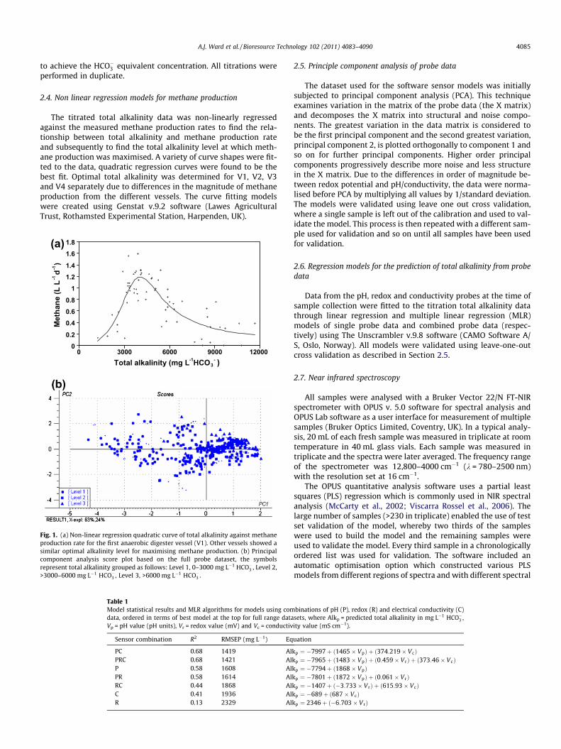
(a)

Fig. 1. (a) Non-linear regression quadratic curve of total alkalinity against methaneproduction rate for the first anaerobic digester vessel (V1). Other vessels showed asimilar optimal alkalinity level for maximising methane production. (b) Principalcomponent analysis score plot based on the full probe dataset, the symbolsrepresent total alkalinity grouped as follows: Level 1, 0–3000 mg L�1 HCO�3 , Level 2,>3000–6000 mg L�1 HCO�3 , Level 3, >6000 mg L�1 HCO�3 .

Table 1Model statistical results and MLR algorithms for models using comdata, ordered in terms of best model at the top for full range dataVp = pH value (pH units), Vr = redox value (mV) and Vc = conductiv

Sensor combination R2 RMSEP (mg L�1) Eq

PC 0.68 1419 AlPRC 0.68 1421 AlP 0.58 1608 AlPR 0.58 1614 AlRC 0.44 1868 AlC 0.41 1936 AlR 0.13 2329 Al

2.5. Principle component analysis of probe data

The dataset used for the software sensor models was initiallysubjected to principal component analysis (PCA). This techniqueexamines variation in the matrix of the probe data (the X matrix)and decomposes the X matrix into structural and noise compo-nents. The greatest variation in the data matrix is considered tobe the first principal component and the second greatest variation,principal component 2, is plotted orthogonally to component 1 andso on for further principal components. Higher order principalcomponents progressively describe more noise and less structurein the X matrix. Due to the differences in order of magnitude be-tween redox potential and pH/conductivity, the data were norma-lised before PCA by multiplying all values by 1/standard deviation.The models were validated using leave one out cross validation,where a single sample is left out of the calibration and used to val-idate the model. This process is then repeated with a different sam-ple used for validation and so on until all samples have been usedfor validation.

2.6. Regression models for the prediction of total alkalinity from probedata

Data from the pH, redox and conductivity probes at the time ofsample collection were fitted to the titration total alkalinity datathrough linear regression and multiple linear regression (MLR)models of single probe data and combined probe data (respec-tively) using The Unscrambler v.9.8 software (CAMO Software A/S, Oslo, Norway). All models were validated using leave-one-outcross validation as described in Section 2.5.

2.7. Near infrared spectroscopy

All samples were analysed with a Bruker Vector 22/N FT-NIRspectrometer with OPUS v. 5.0 software for spectral analysis andOPUS Lab software as a user interface for measurement of multiplesamples (Bruker Optics Limited, Coventry, UK). In a typical analy-sis, 20 mL of each fresh sample was measured in triplicate at roomtemperature in 40 mL glass vials. Each sample was measured intriplicate and the spectra were later averaged. The frequency rangeof the spectrometer was 12,800–4000 cm�1 (k = 780–2500 nm)with the resolution set at 16 cm�1.

The OPUS quantitative analysis software uses a partial leastsquares (PLS) regression which is commonly used in NIR spectralanalysis (McCarty et al., 2002; Viscarra Rossel et al., 2006). Thelarge number of samples (>230 in triplicate) enabled the use of testset validation of the model, whereby two thirds of the sampleswere used to build the model and the remaining samples wereused to validate the model. Every third sample in a chronologicallyordered list was used for validation. The software included anautomatic optimisation option which constructed various PLSmodels from different regions of spectra and with different spectral

binations of pH (P), redox (R) and electrical conductivity (C)sets, where Alkp = predicted total alkalinity in mg L�1 HCO�3 ,ity value (mS cm�1).

uation

kp ¼ �7997þ ð1465� VpÞ þ ð374:219� VcÞkp ¼ �7965þ ð1483� VpÞ þ ð0:459� V rÞ þ ð373:46� VcÞkp ¼ �7794þ ð1868� VpÞkp ¼ �7801þ ð1872� VpÞ þ ð0:061� V rÞkp ¼ �1407þ ð�3:733� V rÞ þ ð615:93� VcÞkp ¼ �689þ ð687� VcÞkp ¼ 2346þ ð�6:703� V rÞ

4086 A.J. Ward et al. / Bioresource Technology 102 (2011) 4083–4090

pre-treatments. The best model was recommended based on min-imising the root mean square error of prediction (RMSEP, the aver-age error of the prediction performed during validation) andmaximising the R2 (variance accounted for by the model) value.

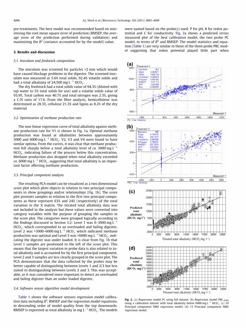
Fig. 2. (a) Regression model PC using full dataset. (b) Regression model PRC<6000

using a calibration dataset with total alkalinity below 6000 mg L�1 HCO�3 . (c) 10Principal component NIRS regression model. (d) 13 Principal component NIRSregression model.

3. Results and discussion

3.1. Inoculum and feedstock composition

The inoculum was screened for particles >2 mm which wouldhave caused blockage problems in the digester. The screened inoc-ulum was measured as 5.6% total solids, 92.4% volatile solids andhad a total alkalinity of 24,500 mg L�1 HCO�3 .

The dry feedstock had a total solids value of 94.3% (diluted withtap water to 5% total solids for use) and a volatile solids value of93.9%. Total carbon was 40.7% and total nitrogen was 2.3%, givinga C:N ratio of 17.6. From the fibre analysis, hemicellulose wasdetermined as 28.3%, cellulose 21.3% and lignin as 8.2% of the drymaterial.

3.2. Optimisation of methane production rate

The non-linear regression curve of total alkalinity against meth-ane production rate for V1 is shown in Fig. 1a. Optimal methaneproduction was found at alkalinities between approximately3000 and 6000 mg L�1 HCO�3 . V2, V3 and V4 were found to havesimilar optima. From the curves, it was clear that methane produc-tion fell sharply below a total alkalinity level of ca. 3000 mg L�1

HCO�3 , indicating failure of the process below this concentration.Methane production also dropped when total alkalinity exceededca. 6000 mg L�1 HCO�3 , suggesting that total alkalinity is an impor-tant factor affecting methane production.

3.3. Principal component analysis

The resulting PCA model can be visualized as a two dimensionalscore plot which plots objects in relation to two principal compo-nents to show groupings and/or relationships (Fig. 1b). The scoreplot presents samples in relation to the first two principal compo-nents as these represent 63% and 24% (respectively) of the totalvariation in the X matrix. The titrated total alkalinity data wasnot included in the analysis but these values were converted intocategory variables with the purpose of grouping the samples inthe score plot. The categories were grouped logically according tothe findings discussed in Section 3.2: Level 1 was 0–3000 mg L�1

HCO�3 , which corresponded to an overloaded and failing digester,Level 2 was >3000–6000 mg L�1 HCO�3 which indicated methaneproduction was optimal and Level 3 was >6000 mg L�1 HCO�3 , indi-cating the digester was under loaded. It is clear from Fig. 1b thatLevel 1 samples are positioned to the left of the score plot. Thismeans that the largest variation in probe data is also related to to-tal alkalinity and is accounted for by the first principal component.Level 2 and 3 samples are less clearly grouped in the score plot. ThePCA demonstrates that the data collected by the probes may bebetter capable of distinguishing between Levels 1 and 2/3 but lesssuited to distinguishing between Levels 2 and 3. This was accept-able, as it was considered more important to detect an overloadedand failing digester than an under loaded digester.

3.4. Software sensor algorithm model development

Table 1 shows the software sensors regression model calibra-tion data including R2, RMSEP and the regression model equations,in descending order of model quality from the top downwards.RMSEP is expressed as total alkalinity in mg L�1 HCO�3 . The models

were named based on the probe(s) used: P for pH, R for redox po-tential and C for conductivity. Fig. 2a shows a predicted versusmeasured plot of the best calibration model, the two probe PCmodel, in terms of R2 and RMSEP. The model statistics and equa-tion (Table 1) are very similar to those of the three probe PRC mod-el suggesting that redox potential played little part when

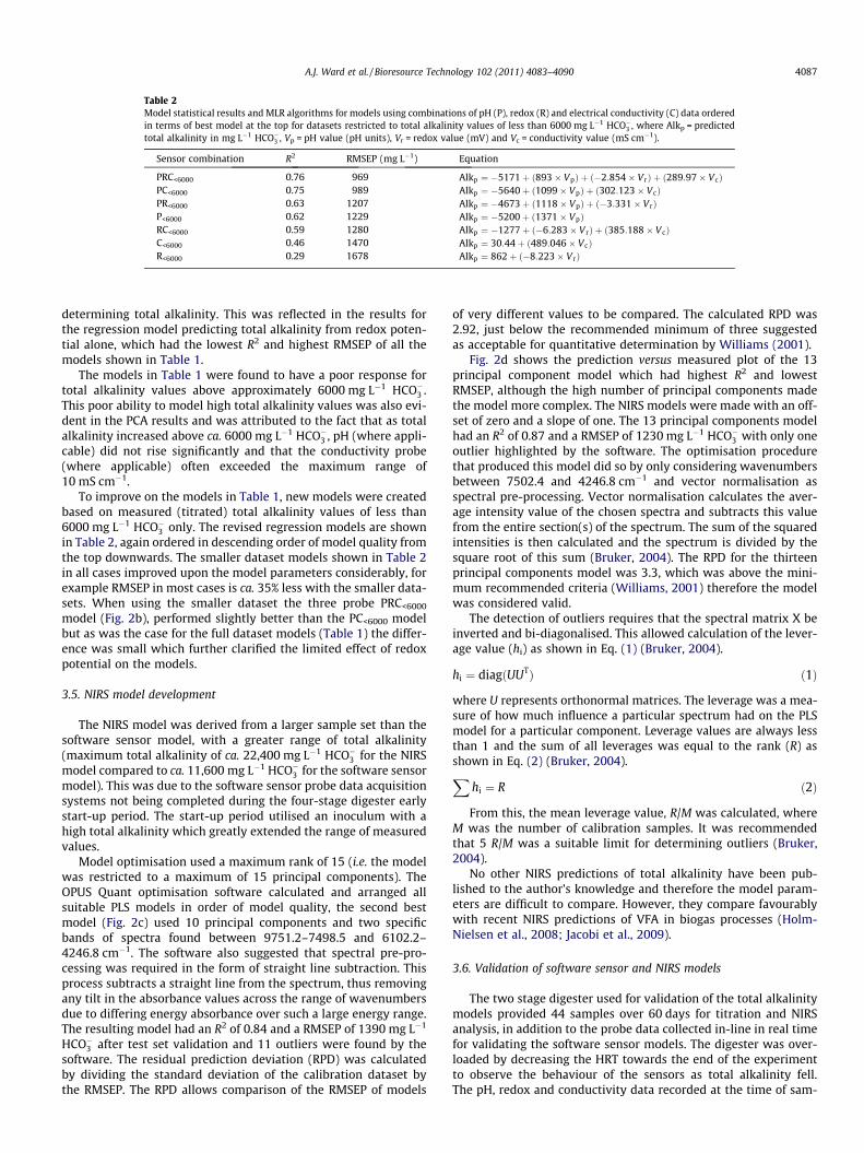
Table 2Model statistical results and MLR algorithms for models using combinations of pH (P), redox (R) and electrical conductivity (C) data orderedin terms of best model at the top for datasets restricted to total alkalinity values of less than 6000 mg L�1 HCO�3 , where Alkp = predictedtotal alkalinity in mg L�1 HCO�3 , Vp = pH value (pH units), Vr = redox value (mV) and Vc = conductivity value (mS cm�1).

Sensor combination R2 RMSEP (mg L�1) Equation

PRC<6000 0.76 969 Alkp ¼ �5171þ ð893� VpÞ þ ð�2:854� V rÞ þ ð289:97� VcÞPC<6000 0.75 989 Alkp ¼ �5640þ ð1099� VpÞ þ ð302:123� VcÞPR<6000 0.63 1207 Alkp ¼ �4673þ ð1118� VpÞ þ ð�3:331� V rÞP<6000 0.62 1229 Alkp ¼ �5200þ ð1371� VpÞRC<6000 0.59 1280 Alkp ¼ �1277þ ð�6:283� V rÞ þ ð385:188� VcÞC<6000 0.46 1470 Alkp ¼ 30:44þ ð489:046� VcÞR<6000 0.29 1678 Alkp ¼ 862þ ð�8:223� V rÞ

A.J. Ward et al. / Bioresource Technology 102 (2011) 4083–4090 4087

determining total alkalinity. This was reflected in the results forthe regression model predicting total alkalinity from redox poten-tial alone, which had the lowest R2 and highest RMSEP of all themodels shown in Table 1.

The models in Table 1 were found to have a poor response fortotal alkalinity values above approximately 6000 mg L�1 HCO�3 .This poor ability to model high total alkalinity values was also evi-dent in the PCA results and was attributed to the fact that as totalalkalinity increased above ca. 6000 mg L�1 HCO�3 , pH (where appli-cable) did not rise significantly and that the conductivity probe(where applicable) often exceeded the maximum range of10 mS cm�1.

To improve on the models in Table 1, new models were createdbased on measured (titrated) total alkalinity values of less than6000 mg L�1 HCO�3 only. The revised regression models are shownin Table 2, again ordered in descending order of model quality fromthe top downwards. The smaller dataset models shown in Table 2in all cases improved upon the model parameters considerably, forexample RMSEP in most cases is ca. 35% less with the smaller data-sets. When using the smaller dataset the three probe PRC<6000

model (Fig. 2b), performed slightly better than the PC<6000 modelbut as was the case for the full dataset models (Table 1) the differ-ence was small which further clarified the limited effect of redoxpotential on the models.

3.5. NIRS model development

The NIRS model was derived from a larger sample set than thesoftware sensor model, with a greater range of total alkalinity(maximum total alkalinity of ca. 22,400 mg L�1 HCO�3 for the NIRSmodel compared to ca. 11,600 mg L�1 HCO�3 for the software sensormodel). This was due to the software sensor probe data acquisitionsystems not being completed during the four-stage digester earlystart-up period. The start-up period utilised an inoculum with ahigh total alkalinity which greatly extended the range of measuredvalues.

Model optimisation used a maximum rank of 15 (i.e. the modelwas restricted to a maximum of 15 principal components). TheOPUS Quant optimisation software calculated and arranged allsuitable PLS models in order of model quality, the second bestmodel (Fig. 2c) used 10 principal components and two specificbands of spectra found between 9751.2–7498.5 and 6102.2–4246.8 cm�1. The software also suggested that spectral pre-pro-cessing was required in the form of straight line subtraction. Thisprocess subtracts a straight line from the spectrum, thus removingany tilt in the absorbance values across the range of wavenumbersdue to differing energy absorbance over such a large energy range.The resulting model had an R2 of 0.84 and a RMSEP of 1390 mg L�1

HCO�3 after test set validation and 11 outliers were found by thesoftware. The residual prediction deviation (RPD) was calculatedby dividing the standard deviation of the calibration dataset bythe RMSEP. The RPD allows comparison of the RMSEP of models

of very different values to be compared. The calculated RPD was2.92, just below the recommended minimum of three suggestedas acceptable for quantitative determination by Williams (2001).

Fig. 2d shows the prediction versus measured plot of the 13principal component model which had highest R2 and lowestRMSEP, although the high number of principal components madethe model more complex. The NIRS models were made with an off-set of zero and a slope of one. The 13 principal components modelhad an R2 of 0.87 and a RMSEP of 1230 mg L�1 HCO�3 with only oneoutlier highlighted by the software. The optimisation procedurethat produced this model did so by only considering wavenumbersbetween 7502.4 and 4246.8 cm�1 and vector normalisation asspectral pre-processing. Vector normalisation calculates the aver-age intensity value of the chosen spectra and subtracts this valuefrom the entire section(s) of the spectrum. The sum of the squaredintensities is then calculated and the spectrum is divided by thesquare root of this sum (Bruker, 2004). The RPD for the thirteenprincipal components model was 3.3, which was above the mini-mum recommended criteria (Williams, 2001) therefore the modelwas considered valid.

The detection of outliers requires that the spectral matrix X beinverted and bi-diagonalised. This allowed calculation of the lever-age value (hi) as shown in Eq. (1) (Bruker, 2004).

hi ¼ diagðUUTÞ ð1Þ

where U represents orthonormal matrices. The leverage was a mea-sure of how much influence a particular spectrum had on the PLSmodel for a particular component. Leverage values are always lessthan 1 and the sum of all leverages was equal to the rank (R) asshown in Eq. (2) (Bruker, 2004).X

hi ¼ R ð2Þ

From this, the mean leverage value, R/M was calculated, whereM was the number of calibration samples. It was recommendedthat 5 R/M was a suitable limit for determining outliers (Bruker,2004).

No other NIRS predictions of total alkalinity have been pub-lished to the author’s knowledge and therefore the model param-eters are difficult to compare. However, they compare favourablywith recent NIRS predictions of VFA in biogas processes (Holm-Nielsen et al., 2008; Jacobi et al., 2009).

3.6. Validation of software sensor and NIRS models

The two stage digester used for validation of the total alkalinitymodels provided 44 samples over 60 days for titration and NIRSanalysis, in addition to the probe data collected in-line in real timefor validating the software sensor models. The digester was over-loaded by decreasing the HRT towards the end of the experimentto observe the behaviour of the sensors as total alkalinity fell.The pH, redox and conductivity data recorded at the time of sam-

Day

0

2000

4000

6000

8000

10000

0 5 10 15 20 25 30 35 40 45 50 55 60 65Tota

l alk

alin

ity

(mg

L -1 H

CO

3- ) ReferenceNIRS rank 10 model

0

2000

4000

6000

8000

10000

0 5 10 15 20 25 30 35 40 45 50 55 60 65Day

Tota

l alk

alin

ity

(mg

L -1 H

CO

3- ) ReferenceNIRS rank 13 model

(a)

(b)

2000

4000

6000

8000

10000

tal a

lkal

inity

(mg

L -1 HCO

3- ) ReferencePRC<6000 model

(c)

4088 A.J. Ward et al. / Bioresource Technology 102 (2011) 4083–4090

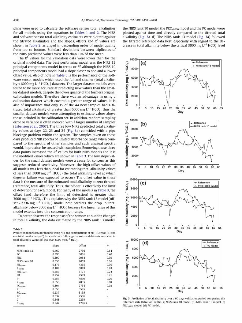
pling were used to calculate the software sensor total alkalinitiesfor all models using the equations in Tables 1 and 2. The NIRSand software sensor total alkalinity estimates were plotted againstthe titrated alkalinities and the slopes, offsets and R2 values areshown in Table 3, arranged in descending order of model qualityfrom top to bottom. Standard deviations between triplicates ofthe NIRS predicted values were less than 10% of the mean.

The R2 values for the validation data were lower than for theoriginal model data. The best performing model was the NIRS 13principal components model in terms or R2 although the NIRS 10principal components model had a slope closer to one and a loweroffset value. Also of note in Table 3 is the performance of the soft-ware sensor models which used the full and smaller (total alkalin-ity < 6000 mg L�1 HCO�3 ) datasets. The larger dataset models werefound to be more accurate at predicting new values than the smal-ler dataset models, despite the lower quality of the formers originalcalibration models. Therefore there was an advantage in using acalibration dataset which covered a greater range of values. It isalso of importance that only 15 of the 44 new samples had a ti-trated total alkalinity of greater than 6000 mg L�1 HCO�3 , thus thesmaller dataset models were attempting to estimate values abovethose included in the calibration set. In addition, random samplingerror or variance is often reduced with a larger number of samples(Esbensen et al., 2007). The three low NIRS predicted total alkalin-ity values at days 22, 23 and 24 (Fig. 3a) coincided with a pipeblockage problem within the system. The samples taken on thesedays produced NIR spectra of limited absorbance range when com-pared to the spectra of other samples and such unusual spectrawould, in practice, be treated with suspicion. Removing these threedata points increased the R2 values for both NIRS models and it isthe modified values which are shown in Table 3. The low slope val-ues for the small dataset models were a cause for concern as thissuggests reduced sensitivity. Moreover, the high offset values ofall models was less than ideal for estimating total alkalinity valuesof less than 3000 mg L�1 HCO�3 (the total alkalinity level at whichdigester failure was expected to occur). The offset value in thesedata is the measure of the estimated total alkalinity at zero titrated(reference) total alkalinity. Thus, the off-set is effectively the limitof detection for each model. For many of the models in Table 3, theoffset (and therefore the limit of detection) is greater than3000 mg L�1 HCO�3 . This explains why the NIRS rank 13 model (off-set = 2736 mg L�1 HCO�3 ) model best predicts the drop in totalalkalinity below 3000 mg L�1 HCO�3 because the linear range of thismodel extends into this concentration range.

To better observe the response of the sensors to sudden changesin total alkalinity, the data estimated by the NIRS rank 13 model,

Table 3Prediction model data for models using NIR and combinations of pH (P), redox (R) andelectrical conductivity (C) data with both full range datasets and datasets restricted tototal alkalinity values of less than 6000 mg L�1 HCO�3 .

Sensor Slope Offset R2

NIRS rank 13 0.460 2736 0.54PC 0.390 3061 0.40PRC 0.390 2984 0.39NIRS rank 10 0.550 2059 0.36PR<6000 0.176 4355 0.30P<6000 0.189 3899 0.28PRC<6000 0.289 3171 0.24PR 0.257 4589 0.21P 0.257 4599 0.20R<6000 0.056 4835 0.08PC<6000 0.304 2734 0.08R 0.050 5585 –RC<6000 0.237 3135 –RC 0.337 2596 –C 0.348 2293 –C<6000 0.247 1776.7 –

the NIRS rank 10 model, the PRC<6000 model and the PC model wereplotted against time and directly compared to the titrated totalalkalinity (Fig. 3a–d). The NIRS rank 13 model (Fig. 3a) followedthe titrated reference data best, especially with regard to the de-crease in total alkalinity below the critical 3000 mg L�1 HCO�3 level

00 5 10 15 20 25 30 35 40 45 50 55 60 65

Day

To

0 5 10 15 20 25 30 35 40 45 50 55 60 650

2000

4000

6000

8000

10000

Day

Tota

l alk

alin

ity (m

g L

-1 H

CO3- ) Reference

PC model(d)

Fig. 3. Prediction of total alkalinity over a 60 days validation period comparing thereference data (titration) with: (a) NIRS rank 10 model, (b) NIRS rank 13 model (c)PRC<6000 model, (d) PC model.

A.J. Ward et al. / Bioresource Technology 102 (2011) 4083–4090 4089

from day 54 onwards. The NIRS rank 10 model (Fig. 3b) performedcomparatively poorly during this period. The poor performance ofthe NIRS rank 10 model was attributed to under fitting of themodel due to too few principal components, i.e. too little of thespectral information was used in the model. Comparing the bestof the small and full dataset calibration models (PRC<6000 and PCmodels, Fig. 3c and d respectively) shows that the full dataset PCmodel gives a better estimate of total alkalinity at the higher levels(above 6000 mg L�1 HCO�3 ) and also at the critical lower level of be-low 3000 mg L�1 HCO�3 . However, none of the software sensormodels performed as well as the NIRS 13 principal componentmodel.

The software sensor was developed as an in-line system fromthe start and scaling up to industrial scale would be a very simpleprocedure at relatively low cost, requiring only the addition of thepH and conductivity probes into an existing anaerobic digestereffluent outlet. The NIRS system described here is an off-line meth-od but could easily be implemented as an in-line method with theuse of a fibre-optic probe positioned in a similar way as describedabove for the software sensor. However, an NIR spectrometer isconsiderably more expensive than the software sensor probes, atca. €50,000 for the former compared to ca. €4000 for the latter.

The strongest point of the two methods of total alkalinity deter-mination described here is their low maintenance and lack of sam-ple preparation rather than their absolute precision and accuracy.Thus, the aim is to track trends in total alkalinity to monitor theprocess and maintain total alkalinity between 3000 and5000 mg L�1 to optimise methane yields. This is actually a broadconcentration range so the main requirement of the model is tobe able to track changes in total alkalinity fast and accurately en-ough to enable rapid corrective action to be taken before methaneyield drops. The NIRS method uses an internal reference systemwhich requires no operator input and the software sensor probesonly required cleaning and calibration every 2 months. Spanjerset al. (2006) found that a sample pre-treatment unit fitted up-stream of a mid-infrared spectrometer was subject to clogging onseveral occasions over a 6 months assessment period, yet bothmethods described here do not require sample pre-treatment.However, the methods described in this paper are not as accurateas other on-line methods described in the literature: Jantsch andMattiasson (2004) achieved a model response with R2 = 0.99 forspiked, filtered effluent samples from a municipal sludge digesterand Hawkes et al. (1993) measured bicarbonate to an accuracy of5% in simulated ice cream waste water using the addition of so-dium bicarbonate or dilution with water to achieve high and lowalkalinities (respectively).

It should be noted that both the software sensor models andthe NIRS model described here could be specific to the feedstockused. It is expected that many intermediates in the anaerobicdigestion process may be similar (for example VFA) but manyother components could change the matrix and without validationon a different feedstock the possibility of universal applicability ofthese models cannot be guaranteed. The NIRS model could be uti-lising a large range of feedstock specific parameters for total alka-linity determination and this may also be the case for theconductivity probe, as the exact mechanism by which total alka-linity affects conductivity has not been fully established. Althoughit is understood that as pH rises above the pka of potentially ioni-sable species these will become ionised leading to an increase inconductivity. However, the concentration of these potentially ioni-sable species is likely to be different in any two digesters fed withdifferent feedstocks, as the measurement of electrical conductivityin the water industry is known to be impossible to compare be-tween different sample sources and, as such, is used only for com-parative measurements from the same water source (HMSO,1978).

4. Conclusions

The software sensor models gave highest R2 = 0.76 (PRC<6000

model). Validation on new samples gave highest R2 = 0.40 (PCmodel). The NIRS model gave improved performance withR2 = 0.87. Validation of the NIRS model on new samples gaveR2 = 0.54. Both methods allowed continuous monitoring but werelimited in accuracy and precision which means that, without fur-ther development, they are only suitable for approximate indica-tions of total alkalinity. However, because the optimum totalalkalinity range for maximum methane production was found tolie between 3000 and 6000 mg L�1 HCO�3 , the NIRS sensor showspromise as an on-line sensor to monitor anaerobic digestionprocesses.

Acknowledgements

The authors would like to thank the European Social Fund andthe UK Biotechnology and Biological Sciences Research Councilfor providing funds for this research.

References

Alcaraz-Gonzalez, V., Harmand, J., Rapaport, A., Steyer, J.P., Gonzalez-Alvarez, V.,Pelayo-Ortiz, C., 2002. Software sensors for highly uncertain waste watertreatment plants: a new approach based on interval observers. Water Research36, 2515–2524.

APHA, 1976. Standard Methods for the Examination of Water and Wastewater, 14ed. APHA, Washington DC.

Barampouti, E.M.P., Mai, S.T., Vlyssides, A.G., 2005. Dynamic modelling of the ratioof volatile fatty acid/bicarbonate alkalinity in a UASB reactor for potatoprocessing wastewater treatment. Environmental Monitoring and Assessment110, 121–128.

Bernard, O., Hadj-Sadok, Z., Dochain, D., 2000. Software sensors to monitor thedynamics of microbial communities: application to anaerobic digestion. ActaBiotheoretica 48, 197–205.

Borja, R., Rincon, B., Raposo, F., Dominguez, J.R., Millan, F., Martin, A., 2004.Mesophilic anaerobic digestion in a fluidised-bed reactor of wastewater fromthe production of protein isolates from chickpea flour. Process Biochemistry 39,1913–1921.

Bruker Spectroscopic Software OPUS Quant, 2004. Bruker Optics Limited, BannerLane, Coventry CV4 9GH, England.

Converti, A., Oliveira, R.P.S., Torres, B.R., Lodi, A., Zilli, M., 2008. Biogas production bymeans of a two-step biological process. Bioresource Technology 100 (23), 5771–5776.

Esbensen, K.H., Friis-Petersen, H.H., Petersen, L., Holm-Nielsen, J.B., Mortensen, P.P.,2007. Representative process sampling – in practice: variographic analysis andestimation of total sampling errors (TSE). Chemometrics and IntelligentLaboratory Systems 88, 41–59.

Feitkenhauer, H., Meyer, U., 2004. Software sensors based on titrimetric techniquesfor the monitoring and control of aerobic and anaerobic bioreactors.Biochemical Engineering Journal 17, 147–151.

Fernandez, N., Montalvo, S., Borja, R., Guerrero, L., Sanchez, E., Cortes, I.,Colmenarejo, M.F., Travieso, L., Raposo, F., 2008. Performance evaluation of ananaerobic fluidized bed reactor with natural zeolite as support material whentreating high-strength distillery wastewater. Renewable Energy 33, 2458–2466.

Ferrer, I., Vazquez, F., Font, F., 2010. Long term operation of a thermophilicanaerobic reactor: process stability and efficiency at decreasing sludgeretention time. Bioresource Technology 101 (9), 2972–2980.

Gizachew, L., Smit, G.N., 2005. Crude protein and mineral composition of major cropresidues and supplemental feeds produced on Vertisols of the Ethiopianhighland. Animal Feed Science and Technology 119, 143–153.

Hansson, M., Nordberg, A., Sundh, I., Mathisen, B., 2002. Early warning ofdisturbances in a laboratory-scale MSW biogas process. Water Science andTechnology 45 (10), 255–260.

Hansson, M., Nordberg, A., Mathisen, B., 2003. On-line NIR monitoring duringanaerobic treatment of municipal solid waste. Water Science and Technology48, 9–13.

Hawkes, F.R., Guwy, A.J., Rozzi, A.G., Hawkes, D.L., 1993. A new instrument foronline measurement of bicarbonate alkalinity. Water Research 27, 167–170.

HMSO, 1978. The Measurement of Electrical Conductivity and the LaboratoryDetermination of the pH Value of Natural, Treated and Waste Waters. HerMajesty’s Stationery Office, London.

Holm-Nielsen, J.B., Lomberg, C.J., Oleskowicz-Popiel, P., Esbensen, K.H., 2008. On-line near infrared monitoring of glycerol-boosted anaerobic digestionprocesses: Evaluation of process analytical technologies. Biotechnology andBioengineering 99, 302–313.

4090 A.J. Ward et al. / Bioresource Technology 102 (2011) 4083–4090

Jacobi, H.F., Moschner, C.R., Hartung, E., 2009. Use of near infrared spectroscopy inmonitoring of volatile fatty acids in anaerobic digestion. Water Science andTechnology 60 (2), 339–346.

Jantsch, T.G., Mattiasson, B., 2003. A simple spectrophotometric method based onpH-indications for monitoring partial and total alkalinity in anaerobicprocesses. Environmental Technology 24, 1061–1067.

Jantsch, T.G., Mattiasson, B., 2004. An automated spectrophotometric system formonitoring buffer capacity in anaerobic digestion processes. Water Research 38,3645–3650.

Kyazze, G., Dinsdale, R., Guwy, A.J., Hawkes, F.R., Premier, G.C., Hawkes, D.L., 2006.Performance characteristics of a two-stage dark fermentative system producinghydrogen and methane continuously. Biotechnology and Bioengineering 97,759–770.

McCarty, G.W., Reeves, J.B., Reeves, V.B., Follett, R.F., Kimble, J.M., 2002. Mid-infrared and near-infrared diffuse reflectance spectroscopy for soil carbonmeasurement. Soil Science Society of America Journal 66, 640–646.

Mendez-Acosta, H.O., Snell-Castro, R., Alcarez-Gonzalez, V., Gonzalez-Alvarez, V.,Pelayo-Ortiz, C., 2010. Anaerobic treatment of Tequila vinasses in a CSTR-typedigester. Biodegradation 21, 357–363.

Moreira, M.B., Ratusznei, S.M., Rodrigues, J.A.D., Zaiat, M., Foresti, E., 2008. Influenceof organic shock loads in an ASBBR treating synthetic wastewater with differentconcentration levels. Bioresource Technology 99, 3256–3266.

Nain, M.Z., Jawed, M., 2006. Performance of anaerobic reactors at low organic loadsubjected to sudden change in feed substrate types. Journal of ChemicalTechnology and Biotechnology 81, 958–965.

Nges, I.A., Liu, J., 2010. Effects of solid retention time on anaerobic digestion ofdewatered-sewage sludge in mesophilic and thermophilic conditions.Renewable Energy 35 (10), 2200–2206.

Spanjers, H., Bouvier, J.C., Steenweg, P., Bisschops, I., van Gils, W.,Versprille, B., 2006. Implementation of in-line infrared monitor infull-scale anaerobic digestion process. Water Science and Technology 53, 55–61.

Steyer, J.P., Bouvier, J.C., Conte, T., Gras, P., Harmand, J., Delgenes, J.P., 2002. On-linemeasurements of COD, TOC, VFA, total and partial alkalinity in anaerobicdigestion processes using infrared spectroscopy. Water Science and Technology45, 133–138.

Van Soest, P.J., Robertson, J.B., Lewis, B.A., 1991. Methods for dietary fiber, neutraldetergent fiber, and nonstarch polysaccharides in relation to animal production.Journal of Dairy Science 74, 3583–3597.

Viscarra Rossel, R.A., Walvoort, D.J.J., McBratney, A.B., Janik, L.J., Skjemstad, J.O.,2006. Visible, near infrared, mid infrared or combined diffuse reflectancespectroscopy for simultaneous assessment of various soil properties. Geoderma131, 59–75.

Ward, A.J., Hobbs, P.J., Holliman, P.J., Jones, D.L., 2008. Optimisation of theanaerobic digestion of agricultural resources. Bioresource Technology 99,7928–7940.

Williams, P.C., 2001. Implementation of near-infrared technology. In: Williams, P.C.,Norris, K. (Eds.), Near-Infrared Technology in the Agricultural and FoodIndustries, Second ed. American Association of Cereal Chemists Inc., St. Paul,Minnesota, USA, pp. 145–169.