Evaluating Mutual Fund Performance

S.P. KothariSloan School of Management

Massachusetts Institute of Technology50 Memorial Drive, Cambridge, MA 02142

E-mail: Kothari@MIT.edu617 253-0994

William E. Simon Graduate School of Business AdministrationUniversity of Rochester, Rochester, NY 14627

and

Jerold B. WarnerWilliam E. Simon Graduate School of Business Administration

University of Rochester, Rochester, NY 14627E-mail: Warner@ssb.rochester.edu

716 275-2678

First draft: August 1997Revised: January 1998

We thank Wayne Ferson, Bill Schwert, Cliff Smith, and seminar participants at the University ofRochester and Duke for their comments, and Peter Wysocki for excellent research assistance.We are grateful to the Research Foundation of the Institute of Chartered Financial Analysts andthe Association for Investment Management and Research, the Bradley Policy Research Centerat the Simon School and the John M. Olin Foundation for financial support.

Abstract

We study standard mutual fund performance measures, using simulation procedures

combined with random and random-stratified samples of NYSE and AMEX securities. We track

simulated fund portfolios over time. These portfolios’ performance is ordinary, and well-

specified performance measures should not indicate abnormal performance. Our main result,

however, is that the performance measures are badly misspecified. Regardless of the

performance measure, there are indications of abnormal fund performance, including market-

timing ability, when none exists.

Evaluating Mutual Fund Performance

1. Introduction

This paper studies empirical properties of performance measures for mutual funds (i.e.,

managed equity portfolios). The portfolio performance evaluation literature is extensive, but

highly controversial. Performance measures based on the Sharpe-Lintner Capital Asset Pricing

Model (CAPM) have a long history and are still used (e.g., Malkiel, 1995, and Ferson and

Schadt, 1996). At the theoretical level, however, there have been strong objections to CAPM-

based measures (e.g., Roll 1977, 1978, Admati and Ross, 1985, and Dybvig and Ross,1985a, b).

For example, the use of a security market line to measure performance can be “ambiguous”

(Roll, 1978, p. 1052). Inference about superior performance using this approach is sometimes

regarded as “hopeless” (Admati and Ross, 1985, p. 16) and “in general anything is possible”

because performance of a manager with superior information can plot “below or above the

security market line and inside or outside of the mean-variance efficient frontier, and any

combination of these is possible” (Dybvig and Ross, 1985a, p. 383).

At the empirical level, asset pricing tests have identified non-beta factors, namely size

(e.g., Banz, 1981) and book-to-market ratio (e.g., Rosenberg, Reid, and Lanstein, 1985, and

Fama and French, 1992), which are relevant in explaining cross-sectional variation in average

returns. In light of such results, some recent studies take into account multiple factors in

evaluating fund performance (e.g., Carhart, 1996). Fama and French (1993, p. 54) argue that the

performance of a managed equity portfolio should be evaluated using a three-factor model

including these additional factors, and they advocate a “simple” and “straightforward” procedure

for doing so.

We provide direct evidence on commonly employed performance measures. We use

simulation procedures, coupled with random and random-stratified samples of NYSE and

AMEX securities. We form simulated fund portfolios and track their performance over time,

using a variety of measures. These portfolios’ performance is ordinary and could be obtained by

uninformed investors. Thus, well-specified performance measures should not indicate abnormal

performance. Our approach differs from mutual fund performance studies. With few exceptions

(e.g., Ferson and Schadt, 1996, p. 448), these studies typically assume the validity of a

2

performance measure, and apply it to observed fund returns. In contrast, we offer independent

evidence on the specification of performance measures.

Our main result is that standard performance measures are misspecified. Regardless of

the performance measure, we find a tendency to detect abnormal fund performance, including

market-timing ability, when none is present. For example, simulated mutual-fund portfolios of

randomly selected stocks exhibit an average abnormal performance (Jensen alpha) of over 3%

per year, which is both statistically and economically significant. Our simulations indicate that

the Fama-French three-factor model’s performance is better than the CAPM’s, but the

corresponding figure for the Fama-French model is -1.2% per year, which is also significant.

The relatively poor performance of CAPM-based measures is not entirely surprising, and we

argue that this performance illustrates known CAPM misspecification. Regardless of the

performance measure, misspecification is particularly troubling with the CRSP value-weighted

index as the benchmark. Ironically, this index is the most commonly used in both the academic

and practitioner literature. We document several sources of misspecification. Misspecification

suggesting inadequacies of the assumed asset-pricing model is present even for the Fama-French

three-factor model. Such results have implications beyond the context of fund performance

evaluation.

We also provide evidence on the ability to detect superior performance. We do not

introduce superior performance into the samples, but our evidence indicates that each

performance measure’s sampling variation is large when performance is ordinary. Thus,

properly specified performance measures will have low power to distinguish superior from

normal performance. Although this point has been suggested elsewhere (e.g., Dybvig and Ross,

1985a and b, and Siegel, 1994, p. 289), we provide evidence on how both power and

specification depend on several variables. Our results are obtained without any underlying

market timing ability, or derivatives use (Jagannathan and Korajczyk, 1986). These

considerations can reduce further the informativeness of fund performance measures.

We examine whether the performance measure misspecifications are related to time-

varying expected market returns and return distributions’ departures from normality, in particular

skewness. The literature identifies several pre-determined information variables that are

correlated with expected market returns. These include dividend yield, book-to-market ratio,

long-term Government bond yield, term premium, and default premium. We find some evidence

3

that Fama-French three-factor-model-based performance measures are significantly related to the

information variables, but the CAPM-based performance measures are not. We find no evidence

to suggest that the portfolio returns’ co-skewness with the market accounts for the observed

performance-measure misspecifications.

Section 2 outlines the issues in measuring fund performance. Section 3 describes our

baseline simulation procedure, including sample construction, portfolio performance measures,

and distributional properties of the performance measures under the null hypothesis. Section 4

discusses results of baseline simulations using mutual funds of randomly-selected stocks.

Section 5 examines the simulation results with stratified-random stock portfolios based on style

(e.g., size, book-to-market). We also provide evidence that simulated fund characteristics

resemble those of actual funds and we argue that our results provide meaningful information for

understanding performance evaluation of these funds. Section 6 examines whether time-varying

expected market returns and portfolio returns’ co-skewness with the market explain the observed

performance-measure misspecifications. Section 7 gives our conclusions.

2. Issues in measuring portfolio performance

We briefly outline key issues in performance evaluation. Since the paper’s main focus is

on test specification, we emphasize issues affecting the properties of the performance

benchmarks in the absence of any abnormal performance.

2.1 Security market lines

We study the use of a security market line, which can represent the assumed asset pricing

benchmark in any model with linear factor pricing. For example, in the Sharpe-Lintner CAPM,

expected returns on assets or portfolios are a linear function of their beta with the market

portfolio. A portfolio’s deviation from this security market line measures abnormal

performance. The deviation is typically estimated by the “Jensen alpha” (Jensen, 1968, 1969),

which is the intercept in a regression of portfolio excess returns against returns on the value-

weighted Index.

The security market line generalizes to multifactor models such as the arbitrage pricing

theory. Asset or portfolio returns are a linear function of factor sensitivities with respect to each

4

nondiversifiable factor in the economy. To implement this benchmark, excess returns can be

regressed against factor returns, and the regression intercept should measure the abnormal return

on the portfolio. In the Fama-French three factor model, the factors are the value-weighted

index, and mimicking portfolios for size and book-to-market factors. These authors argue that

the intercept in this regression should be zero in the absence of any abnormal portfolio

performance.

We investigate properties of the regression intercepts involving both the CAPM (the

Jensen alpha) and the Fama-French model. In both cases, we find that the estimated intercepts

can be systematically nonzero, and are highly sensitive to index choice. These results hold even

for randomly selected portfolios, which do not have unusual size or book to market

characteristics. In addition, the sampling distribution of the intercepts is non-normal, making

inference about performance more complicated than typically assumed.

2.2 Market timing

There is a large literature on market timing. If fund managers have market timing ability,

they will shift portfolios to high beta assets when market returns are expected to be high, and

vice-versa. The resulting nonstationarity in beta will systematically bias downward the Jensen

alpha (Jensen, 1968). Explicit tests for market timing ability have been derived under both

single-factor and multifactor asset pricing benchmarks. Typically, additional terms augment the

security market line to test for market timing ability.

We examine market timing tests. Since by construction our simulations involve no

market timing ability, we should not find any market timing ability. Surprisingly, there are

strong indications of timing ability. We investigate several explanations, and in particular the

relation of market timing tests to time-varying expected returns (see Ferson and Schadt, 1996).

2.3 Reward-risk ratios

We document properties of reward-risk ratios. In particular, portfolio performance is

sometimes measured by its Sharpe ratio, defined as the ratio of market excess returns (over the

riskless rate) to market standard deviation. In the Sharpe-Lintner CAPM, the value-weighted

market portfolio has the highest Sharpe ratio.

5

The Sharpe ratio underlies performance measures for dynamic asset allocation strategies

(e.g., Graham and Harvey, 1997). To evaluate such strategies, benchmark returns are a weighted

average of the riskless and value-weighted market returns having the same standard deviation as

the portfolio under study. The Sharpe ratio is also of interest to practitioners. It is reported by

Morningstar, and is the basis for current risk measurement practice such as the Morgan-Stanley

“M-squared” measure (see the Wall Street Journal, 2/10/97). We illustrate how CAPM

departures can easily yield higher Sharpe ratios than the value-weighted index. Although some

previous literature recognizes this general point (e.g., Grinblatt and Titman, 1987, and

MacKinlay, 1995), our results illustrate the implications of excessive reliance on the value-

weighted index in formulating a mutual fund benchmark.

3. Baseline simulation procedure

This section describes the paper’s baseline simulation procedure. We discuss sample

construction, mutual fund performance measures using alternative expected return models, and

test statistics under the null hypothesis of no abnormal performance. We use standard fund

performance measures found in the literature (e.g., Bodie, Kane, and Marcus (1996, ch. 24)).

The baseline simulations use portfolios of randomly selected stocks. Later, our

sensitivity analysis also uses stratified-random stock portfolios based on style (e.g., size, book-

to-market). The conclusion of misspecification is unchanged. In addition to fund style, the

paper’s simulations make a number of assumptions about portfolio characteristics (e.g., number

of securities, their asset weights in the portfolio, turnover). We also present evidence, based on

Morningstar data, that these simulated fund characteristics resemble those of actual funds. This

increases our confidence that the simulations provide meaningful information for understanding

performance evaluation of these funds.

3.1 Sample construction

We construct a 50-stock mutual fund portfolio each month from January 1964 through

December 1991. We then track these 336 simulated mutual fund portfolios’ performance over

6

three-year periods (months 1 through 36) using a number of performance measures. As

discussed later, these three-year periods are overlapping.

Stock selection. The 50 stocks in each portfolio are selected randomly and without

replacement from the population of all NYSE/AMEX securities having return data on the Center

for Research in Security Prices (CRSP) monthly returns tape. Since the number of NASDAQ

stocks is generally far greater than the number of NYSE/AMEX stocks, inclusion of NASDAQ

stocks in our sampling would have resulted in simulated mutual fund portfolios dominated by

NASDAQ stocks.

Portfolio turnover. While each portfolio’s performance is evaluated over three years, the

portfolio composition is changed at the beginning of the second and third years (i.e., beginning

of months 13 and 25) to mimic turnover in a typical mutual fund. Specifically, we assume 100%

turnover of the stocks in the mutual fund portfolio at the end of each year.

Data availability criteria. Any NYSE/AMEX security with return data available in

month 1 is eligible for inclusion in the portfolio formed at the beginning of month 1, and

similarly any security with return data available in month 13 can be included in the portfolio

formed at the beginning of month 13. Thus, we impose minimal data-availability requirements

in the baseline simulations. For example, only the securities for which return data become

available starting in months 2 through 11 (e.g., initial public offerings) are excluded from the

mutual fund portfolio formed at the beginning of month 1.

Portfolio returns and security weights. For each of the 336 mutual fund portfolios, we

construct a time series of 36 monthly returns starting in month 1. We begin with an equal-

weighted portfolio, but the portfolio is not rebalanced at the end of each month. This is

consistent with the monthly returns earned on a mutual fund that does not trade any of its stocks

in one year. We assume each stock’s dividends are re-invested in the stock. Since we

reconstruct the mutual fund at the beginning of months 13 and 25, we begin the second and third

years with equal-weighted portfolios.

3.2 Portfolio performance measures

7

We apply the following performance measures: Sharpe measure, Jensen alpha, Treynor

measure, appraisal ratio, and Fama-French three-factor model alpha. The finance profession has

used the first four performance measures for many years. The Jensen alpha, the Treynor

measure, and the appraisal ratio are all rooted in the Sharpe-Lintner CAPM, whereas the Fama-

French three-factor alpha is the equivalent of the CAPM-based Jensen alpha in a multi-factor

setting that includes size and book-to-market factors along with the market factor. To evaluate

market timing, we employ two measures: CAPM-based market-timing alpha and gamma and

Fama-French three-factor model-based timing alpha and gamma. Table 1 summarizes the

performance measures and provides a list of selected references for each. Below we briefly

discuss each measure.

[Table 1]

Sharpe measure. The Sharpe measure (see Sharpe, 1966) provides the reward to

volatility trade-off. It is the ratio of the portfolio’s average excess return divided by the standard

deviation of returns:

Sharpe measure = (ARP - ARf)/σP (1)

where ARP = average return on a mutual fund portfolio over the sample period, ARf = average

risk free return over the sample period, and σP = the standard deviation of excess returns over the

sample period.

Jensen alpha. The Jensen alpha measure (see Jensen, 1968, 1969) is the intercept from

the Sharpe-Lintner CAPM regression of portfolio excess returns on the market portfolio excess

returns over the sample period:

RPt - Rft = αP + βP(RMt - Rft) + εPt (2)

where RPt is the mutual fund portfolio return in month t, Rft is the risk free return in month t, RMt

is the return on the market portfolio in month t, εPt is the white noise error term, and αP and βP

are the regression’s intercept and slope (beta risk) coefficients.

Treynor measure. The Treynor measure (see Treynor, 1965) is similar to the Sharpe

measure except that it defines reward (average excess return) as a ratio of the CAPM beta risk:

Treynor measure = (ARP - ARf)/βP . (3)

8

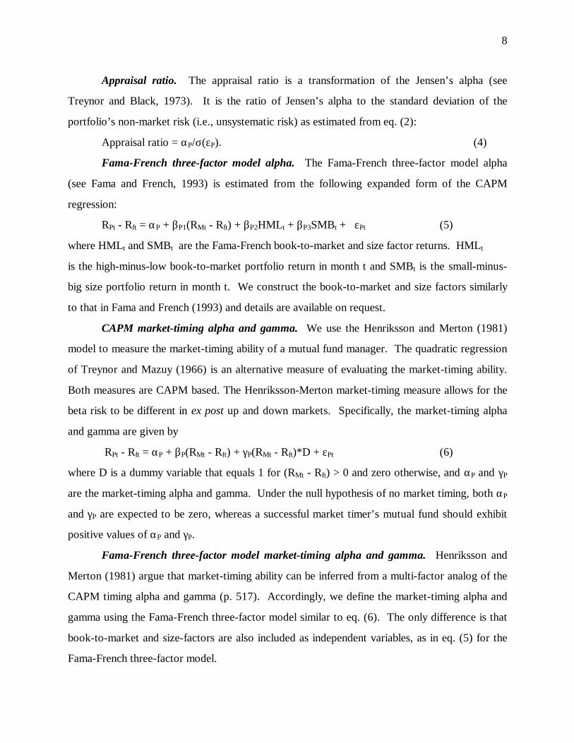
Appraisal ratio. The appraisal ratio is a transformation of the Jensen’s alpha (see

Treynor and Black, 1973). It is the ratio of Jensen’s alpha to the standard deviation of the

portfolio’s non-market risk (i.e., unsystematic risk) as estimated from eq. (2):

Appraisal ratio = αP/σ(εP). (4)

Fama-French three-factor model alpha. The Fama-French three-factor model alpha

(see Fama and French, 1993) is estimated from the following expanded form of the CAPM

regression:

RPt - Rft = αP + βP1(RMt - Rft) + βP2HMLt + βP3SMBt + εPt (5)

where HMLt and SMBt are the Fama-French book-to-market and size factor returns. HMLt

is the high-minus-low book-to-market portfolio return in month t and SMBt is the small-minus-

big size portfolio return in month t. We construct the book-to-market and size factors similarly

to that in Fama and French (1993) and details are available on request.

CAPM market-timing alpha and gamma. We use the Henriksson and Merton (1981)

model to measure the market-timing ability of a mutual fund manager. The quadratic regression

of Treynor and Mazuy (1966) is an alternative measure of evaluating the market-timing ability.

Both measures are CAPM based. The Henriksson-Merton market-timing measure allows for the

beta risk to be different in ex post up and down markets. Specifically, the market-timing alpha

and gamma are given by

RPt - Rft = αP + βP(RMt - Rft) + γP(RMt - Rft)*D + εPt (6)

where D is a dummy variable that equals 1 for (RMt - Rft) > 0 and zero otherwise, and αP and γP

are the market-timing alpha and gamma. Under the null hypothesis of no market timing, both αP

and γP are expected to be zero, whereas a successful market timer’s mutual fund should exhibit

positive values of αP and γP.

Fama-French three-factor model market-timing alpha and gamma. Henriksson and

Merton (1981) argue that market-timing ability can be inferred from a multi-factor analog of the

CAPM timing alpha and gamma (p. 517). Accordingly, we define the market-timing alpha and

gamma using the Fama-French three-factor model similar to eq. (6). The only difference is that

book-to-market and size-factors are also included as independent variables, as in eq. (5) for the

Fama-French three-factor model.

9

3.3 Distributional properties of performance measures

Our research design and data analysis yield a time series of 336 overlapping performance

measure estimates using each of the techniques described in section 3.2. Our objective is to

examine the distributional properties of the estimated performance measures. Under the null

hypothesis of no abnormal performance in the mutual fund portfolios consisting of randomly-

selected stocks, Jensen alpha and Fama-French three-factor model alpha are expected to be zero.

We test the null hypothesis that the time series mean of the Jensen alphas and Fama-French

three-factor model alphas is zero. The test statistic is:

t = (1/T) Σt αt / S.E.(α) (7)

where S.E.(α) is the standard error of the mean of the estimated alphas. If the estimated alphas

are assumed independently distributed, then the standard error is given by:

S.E.(α) = [Σt ( αt - (1/T) Σt αt )2 ]1/2 /(T - 1). (8)

Since the alphas are estimated using 36-month overlapping windows, we use a correction for

serial dependence in estimating the standard error of the mean (see Newey and West, 1987, 1994

and Andrews, 1991) in the calculation of the t-statistic in eq. (7). We also discuss the serial

dependence in the alphas estimated using various models.

Under the null hypothesis, the alpha and the up-market beta in the Henriksson-Merton

market-timing regression model are zero. This holds also in the Fama-French three-factor model

analog of the Henriksson-Merton regression. The test statistic for abnormal performance (i.e.,

alpha = 0) and market-timing ability (i.e., γP from eq. (6) = 0) are similar to that in eq. (7), with

the standard error adjusted using the Newey-West correction for serial dependence.

4. Simulation results

This section reports the paper’s main results. We present distributional properties of

regression-based mutual fund performance measures (e.g., Jensen alpha, the associated t-statistic,

and rejection frequencies) and reward-risk ratios (e.g., the Sharpe measure) for randomly- and

non-randomly selected stock portfolios. The performance measures are often misspecified. The

generally significant misspecifications of the CAPM-based performance measures are reduced,

10

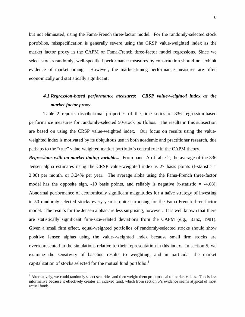
but not eliminated, using the Fama-French three-factor model. For the randomly-selected stock

portfolios, misspecification is generally severe using the CRSP value-weighted index as the

market factor proxy in the CAPM or Fama-French three-factor model regressions. Since we

select stocks randomly, well-specified performance measures by construction should not exhibit

evidence of market timing. However, the market-timing performance measures are often

economically and statistically significant.

4.1 Regression-based performance measures: CRSP value-weighted index as the

market-factor proxy

Table 2 reports distributional properties of the time series of 336 regression-based

performance measures for randomly-selected 50-stock portfolios. The results in this subsection

are based on using the CRSP value-weighted index. Our focus on results using the value-

weighted index is motivated by its ubiquitous use in both academic and practitioner research, due

perhaps to the “true” value-weighted market portfolio’s central role in the CAPM theory.

Regressions with no market timing variables. From panel A of table 2, the average of the 336

Jensen alpha estimates using the CRSP value-weighted index is 27 basis points (t-statistic =

3.08) per month, or 3.24% per year. The average alpha using the Fama-French three-factor

model has the opposite sign, -10 basis points, and reliably is negative (t-statistic = -4.68).

Abnormal performance of economically significant magnitudes for a naïve strategy of investing

in 50 randomly-selected stocks every year is quite surprising for the Fama-French three factor

model. The results for the Jensen alphas are less surprising, however. It is well known that there

are statistically significant firm-size-related deviations from the CAPM (e.g., Banz, 1981).

Given a small firm effect, equal-weighted portfolios of randomly-selected stocks should show

positive Jensen alphas using the value--weighted index because small firm stocks are

overrepresented in the simulations relative to their representation in this index. In section 5, we

examine the sensitivity of baseline results to weighting, and in particular the market

capitalization of stocks selected for the mutual fund portfolio.1

1 Alternatively, we could randomly select securities and then weight them proportional to market values. This is lessinformative because it effectively creates an indexed fund, which from section 5’s evidence seems atypical of mostactual funds.

11

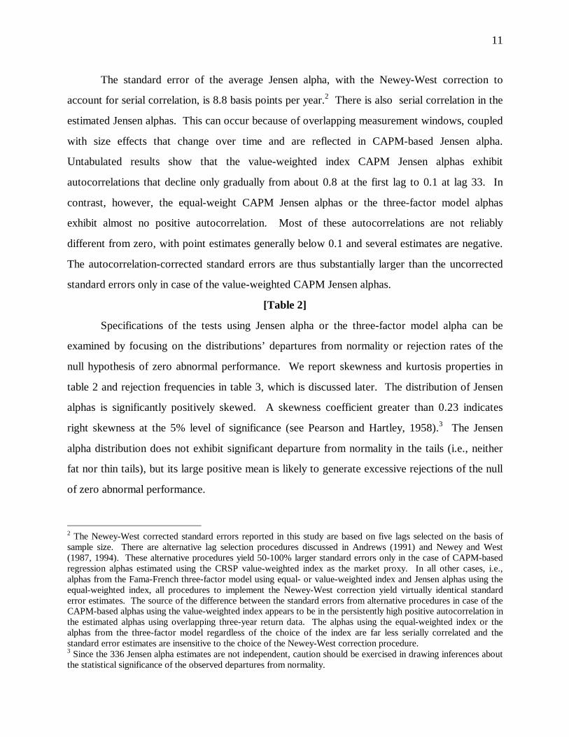
The standard error of the average Jensen alpha, with the Newey-West correction to

account for serial correlation, is 8.8 basis points per year.2 There is also serial correlation in the

estimated Jensen alphas. This can occur because of overlapping measurement windows, coupled

with size effects that change over time and are reflected in CAPM-based Jensen alpha.

Untabulated results show that the value-weighted index CAPM Jensen alphas exhibit

autocorrelations that decline only gradually from about 0.8 at the first lag to 0.1 at lag 33. In

contrast, however, the equal-weight CAPM Jensen alphas or the three-factor model alphas

exhibit almost no positive autocorrelation. Most of these autocorrelations are not reliably

different from zero, with point estimates generally below 0.1 and several estimates are negative.

The autocorrelation-corrected standard errors are thus substantially larger than the uncorrected

standard errors only in case of the value-weighted CAPM Jensen alphas.

[Table 2]

Specifications of the tests using Jensen alpha or the three-factor model alpha can be

examined by focusing on the distributions’ departures from normality or rejection rates of the

null hypothesis of zero abnormal performance. We report skewness and kurtosis properties in

table 2 and rejection frequencies in table 3, which is discussed later. The distribution of Jensen

alphas is significantly positively skewed. A skewness coefficient greater than 0.23 indicates

right skewness at the 5% level of significance (see Pearson and Hartley, 1958).3 The Jensen

alpha distribution does not exhibit significant departure from normality in the tails (i.e., neither

fat nor thin tails), but its large positive mean is likely to generate excessive rejections of the null

of zero abnormal performance.

2 The Newey-West corrected standard errors reported in this study are based on five lags selected on the basis ofsample size. There are alternative lag selection procedures discussed in Andrews (1991) and Newey and West(1987, 1994). These alternative procedures yield 50-100% larger standard errors only in the case of CAPM-basedregression alphas estimated using the CRSP value-weighted index as the market proxy. In all other cases, i.e.,alphas from the Fama-French three-factor model using equal- or value-weighted index and Jensen alphas using theequal-weighted index, all procedures to implement the Newey-West correction yield virtually identical standarderror estimates. The source of the difference between the standard errors from alternative procedures in case of theCAPM-based alphas using the value-weighted index appears to be in the persistently high positive autocorrelation inthe estimated alphas using overlapping three-year return data. The alphas using the equal-weighted index or thealphas from the three-factor model regardless of the choice of the index are far less serially correlated and thestandard error estimates are insensitive to the choice of the Newey-West correction procedure.3 Since the 336 Jensen alpha estimates are not independent, caution should be exercised in drawing inferences aboutthe statistical significance of the observed departures from normality.

12

The estimated Jensen alphas range from -1.28 to 2.69% per month. The large standard

deviation and the wide range even in the absence of abnormal performance are indications that

Jensen alpha, even if properly specified, will have low power to distinguish superior from normal

performance. The Fama-French 3-factor alphas have a lower standard deviation, and a narrower

range, -1.57 to 1.01. This is expected, given the additional explanatory power of size and book-

to-market. Abnormal performance of economically large magnitudes in a 50-stock portfolio is

still not easily detectable, however.

The magnitudes of average annual abnormal performance of 3.2% and -1.2% indicated

by the CAPM and the Fama-French model are comparable in absolute magnitude to a typical

mutual fund’s abnormal performance reported in the literature. For example, Malkiel (1995,

table III) estimates an average Jensen alpha using returns before expenses of 239 general equity

funds from 1982-1991 to be -2% per year. Employing a number of arbitrage portfolio theory

factor models, Lehmann and Modest (1987) estimate abnormal performance of approximately -3

to -4% per year using returns after expenses for 130 mutual funds from 1968 to 1982. They

conclude that either the average mutual fund significantly under-performs or that inferences

about performance are sensitive to “the choice of what constitutes normal performance” (p. 263).

Since we find that the CAPM and three-factor models indicate abnormal performance

magnitudes using random portfolios that are similar to those reported in the literature using

actual mutual fund portfolio returns, popularly used performance measures appear incapable of

distinguishing a mutual fund manager’s superior from ordinary performance and/or skill.

Regressions with market timing variables. Panel A shows that the CAPM-based

Henriksson and Merton (1981) test of market timing is severely misspecified. Using the value-

weighted portfolio, the average market timing alpha for the portfolio of randomly-selected 50

stocks is a whopping 63 basis points per month or 7.6% per year (t-statistic = 4.95). Even

though there is no market timing in the simulations, the estimated average market-timing gamma

is -0.22 (t-statistic = -4.19). The Fama-French three-factor-model-based tests of market timing

exhibit a moderate degree of misspecification. The average timing alpha is -7 basis points (t-

statistic = -1.70) and the average timing gamma of -0.03 is indistinguishable from zero. Greater

misspecification of the market-timing tests compared to the Jensen-alpha tests suggests that

13

omitted determinants of expected returns, departures from normality (e.g., skewness) and/or

changing expected rates of returns might be the contributing factors. We explore these

explanations in section 5.

4.2 Regression-based performance measures: CRSP equal-weighted index as the

market-factor proxy.

Although not generally to used evaluate mutual fund performance, we also report results

using the CRSP equal-weighted index as the market factor proxy. The use of the equal-weighted

index might mitigate any size-related Jensen-alpha misspecifications. The observed

misspecifications are unlikely to be entirely related to firm size, however, because performance

measures based on the Fama-French three-factor model, that explicitly includes a size factor,

were also misspecified.

No market timing. From panel B, consistent with the expectation of lesser

misspecification, the average Jensen alpha and the Fama-French three-factor model alpha are one

basis point or less in absolute magnitude and statistically indistinguishable from zero. The

distribution is significantly right skewed and fat tailed, but the results in table 3 suggest

departures from normality are not large enough to produce test misspecification using the Jensen

alpha performance measure. Since we construct portfolios from randomly-selected stocks, not

surprisingly, Jensen alphas using the equal-weighted index are close to zero. However, as seen

below, the use of an equal-weighted market factor proxy still yields poorly-specified market

timing tests. These results using the equal-weighted index are especially troubling because they

illustrate that there is misspecification even when security weights in portfolios are directly

proportional to their weights in the market index.

Market timing. The market-timing tests using both CAPM and the three-factor model

are quite misspecified. The CAPM-based average market-timing alpha is 19 basis points per

month or 2.3% per year. The Fama-French three-factor model also yields an average market

timing alpha of similar magnitude. In both cases the average alphas are statistically highly

significant. To counterbalance the estimated average positive timing alphas in the regressions,

the timing gammas are on average negative. They are -0.10 (t-statistic = -6.47) using the CAPM

14

and -0.08 (t-statistic = -5.66) using the three-factor model. Thus, commonly-used methods tend

to conclude that a buy-and-hold strategy exhibits negative market-timing ability.

Raw performance measures. Panel C of table 2 reports average monthly returns on the

value- and equal-weighted indexes and the portfolio of randomly-selected stocks. The averages

are calculated from the time series of 336 overlapping three-year average monthly returns. The

grand mean of the 336 three-year average returns for the value-weighted index is 0.93% return

per month with a standard deviation of 0.57%. The corresponding figures for the randomly-

selected 50-stock portfolios are 1.26% and 0.94%. The difference is not surprising because

larger, less risky stocks dominate the value-weighted index. The average return on the CRSP

equal-weighted index is 1.26% with a standard deviation of 0.94% per month. As expected, this

is comparable to the average return and standard deviation of the portfolios of 50 randomly-

selected stocks. This in part explains the lack of misspecification of the performance measures

using the equal-weighted index. That is, tests with no market-timing variables are well-specified

when the sample portfolio by construction mimics the index in virtually every dimension.

4.3 Test statistics and rejection frequencies of regression-based tests of performance

Table 3 reports distributional properties of the test statistics from the 336 CAPM and

three-factor model regressions using the equal- and value-weighted indexes with and without

market timing. To focus on the tail regions of the distributions, table 3 also reports rejection

rates of the null hypothesis of zero abnormal performance or of no market timing ability. The

results in table 3 reinforce those in table 2 and the misspecification of the performance measure

can be dramatic.

From panel A, the average t-statistics are generally large in absolute magnitude when the

regressions employed the CRSP value-weighted index. For example, the average t-statistic for

the Jensen alphas is 0.43 (standard deviation = 1.42) and for the timing alphas it is 0.82 (standard

deviation = 1.34). The standard deviations of the distributions of t-statistics are considerably

greater than 1 for the Jensen alpha and the market-timing alpha using the value-weighted index.4

If the tests were well-specified, the mean (standard deviation) of the distribution of t-statistics

4 Since the regressions use overlapping return data, the reported standard deviation likely understates the truestandard deviation that would be applicable for a sample of 336 independent estimates of t-statistics.

15

should be zero (one). Panel B shows that the positive means and fat-tailed distributions of t-

statistics for the Jensen alphas and CAPM timing alphas generate excessive rates of rejections of

the null hypothesis in favor of positive abnormal performance. The CAPM timing alpha is

significantly positive at the 5% level of significance 27.7% of the time.

[Table 3]

Panel B shows that, using the equal-weighted index, both the CAPM and the three-factor

model timing alphas indicate positive abnormal performance moderately too often (11.6% and

9.8% compared to an expected rate of 5%). The CAPM timing gamma using both equal- and

value-weighted index and the three-factor model timing gamma using the equal-weighted index

also exhibit too many rejections in favor of negative market timing.

4.4 Reward-risk ratios

The central prediction of the Sharpe-Lintner CAPM is that ex ante the value-weighted

market portfolio has the highest Sharpe ratio. Table 4 reports descriptive statistics on reward-to-

risk ratios for the value- and equal-weighted indexes and the 336 simulated portfolios of

randomly-selected stocks.

Contrary to the CAPM prediction, mutual fund the Sharpe ratios of the CRSP equal-

weighted index and the portfolio of randomly-selected stocks substantially exceed the Sharpe

ratio of the CRSP value-weighted index. The average Sharpe ratio of the value-weighted index

is only 0.10, compared to 0.14 for the equal-weighted index and 0.13 for the simulated portfolio

of randomly-selected stocks. This finding is not driven by extreme observations. Median Sharpe

ratios yield the same inference. Given well-documented size-related inadequacies of the CAPM,

these results are expected. These inadequacies make it less probable that the value-weighted

index was ex ante efficient, but that the equal-weighted index simply performed better ex post

than the value-weighted index in the 28-year sample period.5

[Table 4]

The Treynor measure uses beta in the denominator of the ratio, unlike the Sharpe

measure, which uses total volatility. Since betas (which are given an equal-weight in our

5 The Sharpe ratio of the CRSP equal-weighted index is greater than that of the CRSP value-weighted index over amuch longer period beginning in 1926. This makes it less likely that the higher Sharpe ratio of the equal-weightedindex over the 28-year sample period examined in this study is a period-specific phenomenon.

16

mutual-fund portfolios) estimated against the value-weighted index are generally greater than

those estimated against the equal-weighted index, one expects the Treynor measure using the

value-weighted index to exceed that using the equal-weighted index.6 Table 4, however, shows

that the Treynor measure for the portfolios of randomly-selected stocks using the value-weighted

index betas is 0.63 compared to 0.72 using the equal-weighted index betas. These results are

consistent with a lower Sharpe ratio of the value-weighted index than that of the equal-weighted

index.

The appraisal ratios using the equal- and value-weighted indexes provide conflicting

inferences. The appraisal ratio of the random-stocks portfolio using the value-weighted index is

0.07 (t-statistic 2.47) compared to -0.02 (t-statistic -1.60) using the equal-weighted index.

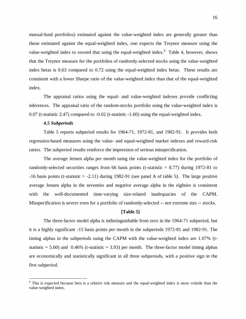
4.5 Subperiods

Table 5 reports subperiod results for 1964-71, 1972-81, and 1982-91. It provides both

regression-based measures using the value- and equal-weighted market indexes and reward-risk

ratios. The subperiod results reinforce the impression of serious misspecification.

The average Jensen alpha per month using the value-weighted index for the portfolio of

randomly-selected securities ranges from 66 basis points (t-statistic = 8.77) during 1972-81 to

-16 basis points (t-statistic = -2.11) during 1982-91 (see panel A of table 5). The large positive

average Jensen alpha in the seventies and negative average alpha in the eighties is consistent

with the well-documented time-varying size-related inadequacies of the CAPM.

Misspecification is severe even for a portfolio of randomly-selected -- not extreme size -- stocks.

[Table 5]

The three-factor model alpha is indistinguishable from zero in the 1964-71 subperiod, but

it is a highly significant -15 basis points per month in the subperiods 1972-81 and 1982-91. The

timing alphas in the subperiods using the CAPM with the value-weighted index are 1.07% (t-

statistic = 5.60) and 0.46% (t-statistic = 3.93) per month. The three-factor model timing alphas

are economically and statistically significant in all three subperiods, with a positive sign in the

first subperiod.

6 This is expected because beta is a relative risk measure and the equal-weighted index is more volatile than thevalue-weighted index.

17

Panel B shows that the use of the equal-weighted index eliminates the misspecification of

the Jensen alpha and the three-factor model alpha. The average Jensen alphas range from -7 to 3

basis points per month and the three-factor model alphas average -3 to 4 basis points per month

in the three subperiods. These are fairly small economically and in all but one case statistically

insignificant. The CAPM and the three-factor model timing alphas, however, continue to be

significantly non-zero, but their magnitudes are muted compared to those observed using the

value-weighted index. Both the models yield timing alphas that are consistently positive in all

three subperiods. To offset the effect of positive timing alphas in the regression, the market

timing gammas are consistently negative.

5. Sensitivity analysis

5.1 Style (non-random) portfolios

Results so far show that even when equity portfolios have no systematically unusual

characteristics, i.e., no particular style, performance measures are misspecified. Therefore, our

priors are that performance measures for style portfolios (i.e., portfolios formed on stock

characteristics such as size and book-to-market) will also be misspecified. Because there is wide

cross-sectional variation in funds’ asset characteristics, it is especially important to understand

how misspecification is related to fund style. In addition, results using non-randomly selected

stocks could provide clues about the underlying determinants of the misspecification.

Size portfolios. Table 6 reports results for large- (panel A) and small-capitalization stock

portfolios (panel B) using the CRSP value-weighted index as the market-factor proxy. Large

(small) stocks are defined as those belonging to CRSP market-capitalization deciles 8-10 (deciles

1-3), where the decile rankings are based only on NYSE stocks’ market capitalizations.

The Jensen alpha and Fama-French three-factor model alpha of the large-stock portfolios

are quite small, 5 and -2 basis points per month, respectively. The corresponding alphas of the

small-stock portfolios are statistically and economically significantly non-zero, however.

Consistent with the size effect, the Jensen alpha of the small-stock mutual fund portfolios is 50

basis points (t-statistic = 3.23) per month. Interestingly, the Fama-French three-factor alpha is

18

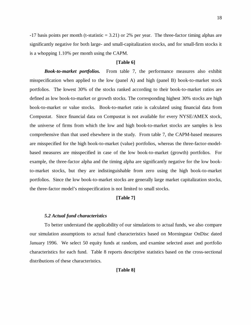
-17 basis points per month (t-statistic = 3.21) or 2% per year. The three-factor timing alphas are

significantly negative for both large- and small-capitalization stocks, and for small-firm stocks it

is a whopping 1.10% per month using the CAPM.

[Table 6]

Book-to-market portfolios. From table 7, the performance measures also exhibit

misspecification when applied to the low (panel A) and high (panel B) book-to-market stock

portfolios. The lowest 30% of the stocks ranked according to their book-to-market ratios are

defined as low book-to-market or growth stocks. The corresponding highest 30% stocks are high

book-to-market or value stocks. Book-to-market ratio is calculated using financial data from

Compustat. Since financial data on Compustat is not available for every NYSE/AMEX stock,

the universe of firms from which the low and high book-to-market stocks are samples is less

comprehensive than that used elsewhere in the study. From table 7, the CAPM-based measures

are misspecified for the high book-to-market (value) portfolios, whereas the three-factor-model-

based measures are misspecified in case of the low book-to-market (growth) portfolios. For

example, the three-factor alpha and the timing alpha are significantly negative for the low book-

to-market stocks, but they are indistinguishable from zero using the high book-to-market

portfolios. Since the low book-to-market stocks are generally large market capitalization stocks,

the three-factor model’s misspecification is not limited to small stocks.

[Table 7]

5.2 Actual fund characteristics

To better understand the applicability of our simulations to actual funds, we also compare

our simulation assumptions to actual fund characteristics based on Morningstar OnDisc dated

January 1996. We select 50 equity funds at random, and examine selected asset and portfolio

characteristics for each fund. Table 8 reports descriptive statistics based on the cross-sectional

distributions of these characteristics.

[Table 8]

19

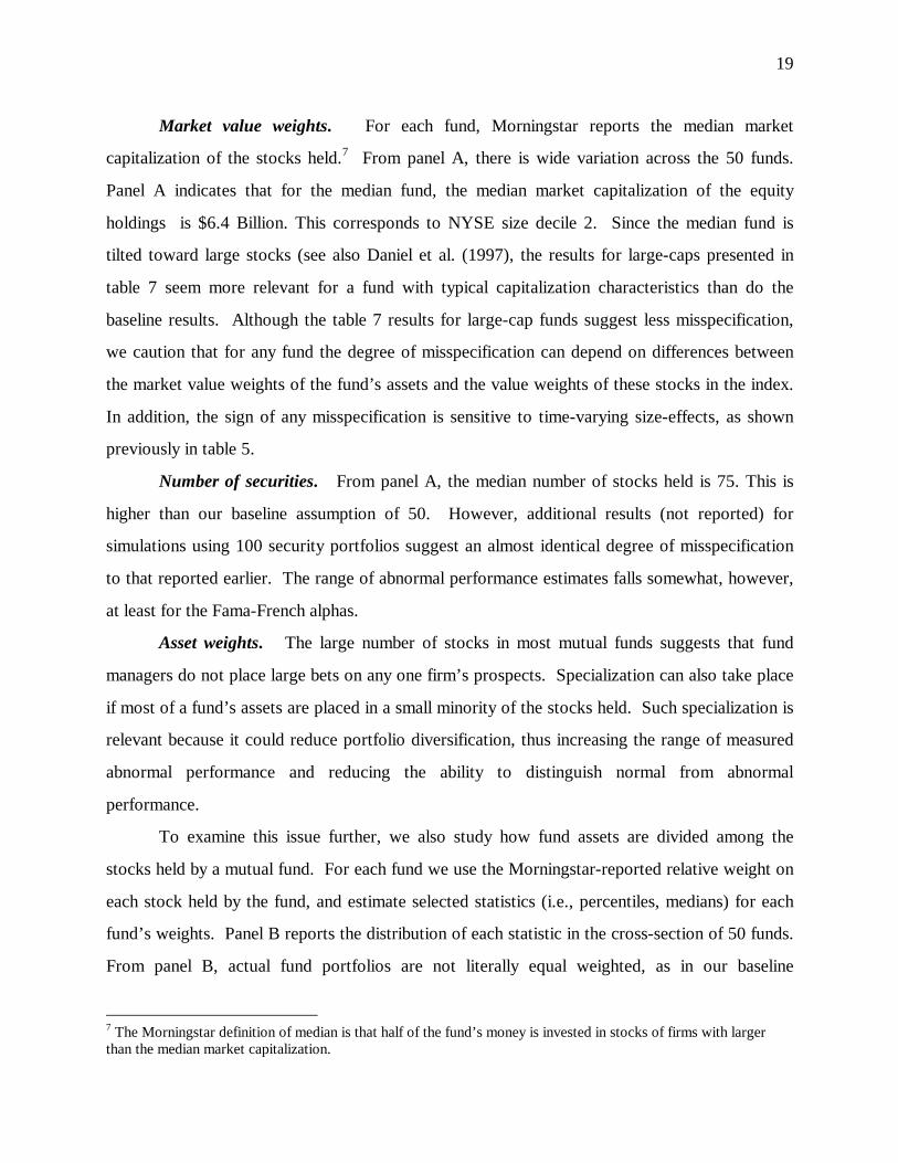
Market value weights. For each fund, Morningstar reports the median market

capitalization of the stocks held.7 From panel A, there is wide variation across the 50 funds.

Panel A indicates that for the median fund, the median market capitalization of the equity

holdings is $6.4 Billion. This corresponds to NYSE size decile 2. Since the median fund is

tilted toward large stocks (see also Daniel et al. (1997), the results for large-caps presented in

table 7 seem more relevant for a fund with typical capitalization characteristics than do the

baseline results. Although the table 7 results for large-cap funds suggest less misspecification,

we caution that for any fund the degree of misspecification can depend on differences between

the market value weights of the fund’s assets and the value weights of these stocks in the index.

In addition, the sign of any misspecification is sensitive to time-varying size-effects, as shown

previously in table 5.

Number of securities. From panel A, the median number of stocks held is 75. This is

higher than our baseline assumption of 50. However, additional results (not reported) for

simulations using 100 security portfolios suggest an almost identical degree of misspecification

to that reported earlier. The range of abnormal performance estimates falls somewhat, however,

at least for the Fama-French alphas.

Asset weights. The large number of stocks in most mutual funds suggests that fund

managers do not place large bets on any one firm’s prospects. Specialization can also take place

if most of a fund’s assets are placed in a small minority of the stocks held. Such specialization is

relevant because it could reduce portfolio diversification, thus increasing the range of measured

abnormal performance and reducing the ability to distinguish normal from abnormal

performance.

To examine this issue further, we also study how fund assets are divided among the

stocks held by a mutual fund. For each fund we use the Morningstar-reported relative weight on

each stock held by the fund, and estimate selected statistics (i.e., percentiles, medians) for each

fund’s weights. Panel B reports the distribution of each statistic in the cross-section of 50 funds.

From panel B, actual fund portfolios are not literally equal weighted, as in our baseline

7 The Morningstar definition of median is that half of the fund’s money is invested in stocks of firms with largerthan the median market capitalization.

20

simulations, but funds do not appear to weight heavily toward only a few assets. Across the 50

funds, the typical (i.e., median) maximum asset weight is only 2.82%; the typical median asset

weight 0.85%, and the typical 90th percentile of a fund’s weights is only 1.68%.

Turnover. Median annual turnover from our sample of Morningstar funds is 47.5%. This

is lower than the 100% figure assumed in the simulations. It is unclear exactly how turnover

would be expected to affect the simulations. Nevertheless, we also performed simulations under

other assumptions about turnover, but there was no difference in the paper’s results.

Trading costs. Our simulations use gross returns. Like all standard procedures, we

measure performance compared to a benchmark, which implicitly assumes a buy-and-hold

strategy. An additional consideration is that fund managers cannot always follow a buy-and-hold

strategy in the face of unexpected inflows or outflows. Edelen (1996) argues that liquidity

trading associated with these flows generates price concessions and reduces the observed gross

returns of funds. Although we have not adjusted downward the gross fund returns to reflect any

such liquidity costs, the magnitude of the adjustments developed in Edelen (1996) is small

relative to the cross-sectional variation in measured abnormal performance reported here.

Further, although Edelen (1996) argues that apparent regularities such as fund managers’

negative market-timing ability could be due to the failure of standard measures to incorporate

liquidity costs, our evidence suggests that misspecification occurs with no such costs.

6. Exploring causes of test misspecification: Time-varying expected returns and

co-skewness

In this section we perform an exploratory analysis of whether the test misspecification

documented in the previous section are explained by time-varying expected returns and/or

departures from normality, in particular, coskewness. Neither appears to substantially account

for the performance measure misspecification. There is only weak evidence that the simulated

mutual fund portfolios’ estimated performance measures covary with proxies for time-variation

in market expected returns, particularly the book-to-market ratio. We do not find co-skewness to

be systematically associated with the estimated performance measures.

21

6.1 Association of performance measures with variables proxying for the market

expected return

In our simulated mutual fund portfolios, the null hypothesis of no market timing is true

and performance measures are not expected to show market timing. However, the existing

performance measures assume stationary expected market (or factor) returns and constant factor

sensitivities of the mutual fund portfolios. Both could change through time, thus potentially

inducing test misspecification. Although we do not know the exact relation, one means of

examining whether changing expected market returns induce misspecification is to test for a

relation between the performance measures and predetermined variables that are correlated with

expected market returns.

Our approach complements the emerging literature that seeks to uncover the effect of

mutual fund managers’ market-timing ability that might be related to time-varying expected

market return as inferred from observable indicators like the dividend yield or term premium

(see, for example, Ferson and Schadt, 1996, Glosten and Jagannathan, 1994, and Chen and Knez,

1996). Ferson and Schadt (1996) infer mutual fund managers’ market-timing ability from the

relation between the mutual funds’ risks and variables correlated with expected market returns.

Ferson and Schadt make the usual assumption that in the absence of market timing and time-

varying expected returns the mutual fund performance measures are well specified. Our

objective is to ascertain whether reported market-timing results for actual funds could be in part

a manifestation of the observed performance measure misspecification.

We regress the time series of 336 estimated performance measures (i.e., estimated alphas

from the CAPM and the Fama-French three-factor models without market timing, and estimated

alphas and betas from these two models with market timing) on a set of pre-determined

information variables that previous literature has shown to be correlated with time variation in

expected market returns (e.g., Fama and French, 1989, Ferson and Harvey, 1991, Breen, Glosten,

and Jagannathan, 1989, and Evans, 1994). The information variables we use are dividend yield

on the NYSE-AMEX value-weighted portfolio, book-to-market ratio of the value-weighted

NYSE-AMEX stocks (for which book value of equity data are available on COMPUSTAT), ten-

22

year Government bond yield, term premium measured as the difference between the ten-year

bond yield and the one-month T-bill interest rate, and default premium measured as the

difference between the junk-bond yield and the 10-year Government bond yield. We also

entertained additional information variables like the price-earnings ratio, one-month T-bill

interest rate, and default premium defined as the difference between BAA and AAA corporate

bond yields. Neither individually nor collectively did they add significantly to the reported

results, so we omit those from the tabulated results.

Table 9 reports the results using the value-weighted index as the market-factor proxy

employed in estimating various performance measures. We obtain results that are qualitatively

similar to those reported below using the equal-weighted index. Since the performance measures

are estimated using returns for overlapping three-year periods, the residuals from the regressions

of performance measures on the information variables are likely to be autocorrelated. This is

confirmed by the observed low values of the Durbin-Watson statistic. We re-estimate the

models that had significant Durbin-Watson statistic by fitting a first- and second-order

autoregressive process on the errors. The Durbin-Watson statistic of the regression models using

the transformed variables is close to 2 and statistically insignificant.

Panel A contains results using performance measures for the simulated portfolios

consisting randomly-selected 50 stocks. The CAPM-based alphas with and without market

timing do not exhibit a statistically reliable evidence of covariation between the performance

measures and market expected return proxies. The CAPM market-timing gamma is positively

related to book-to-market and negatively related to default premium at the 5% significance level

and dividend yield is significant at the 10% level. The opposite signs on the coefficients on

dividend yield and book-to-market are surprising because expected market returns increase in

both these variables (e.g., Fama and French, 1989, and Kothari and Shanken, 1997). The

significant relation between the timing gammas and the information variables in the absence of

true market timing in the simulations raises questions about the interpretation of similar

associations using mutual fund return data (e.g., Ferson and Schadt, 1996). It appears that a

portion of the observed association between information variables and market-timing gammas

using mutual fund return data might be due to model misspecification. Panel A also shows that

23

the Fama-French three-factor model alphas with and without timing are significantly negatively

associated with book-to-market, term premium, and default premium. The timing gammas,

however, do not exhibit significant covariation with the information variables.

[Table 9]

Panels B and C report results for stratified random samples of large and small firms and

panels D and E report results for the high and low book-to-market stock portfolios. These results

indicate that the small firms and high book-to-market portfolios’ three-factor model alphas are

reliably negatively correlated with the book-to-market ratio and default premium. The results

suggest that in high expected market return periods the three-factor model is likely to

erroneously indicate under-performance of small and high book-to-market stocks, and

conversely, above-normal performance in low expected market return periods.

Except for the large stock portfolios, the three-factor model timing gammas are reliably

correlated with dividend yield and default premium. However, the associations between

performance measures and the information variables do not appear to entirely explain the

misspecifications noted in tables 6 and 7. There we find that the three-factor model is

misspecified in the case of low, not high, book-to-market stock portfolios. Panels B through E

show that there is limited evidence of the CAPM-based performance measures, with and without

timing, being associated with the information variables.

6.2 Association of performance measures with coskewness

The observed performance measure misspecification could be related to the return

distributions’ departures from normality. First, departures from joint normality of the mutual

fund portfolio returns and market returns could distort the performance measures’ sampling

distribution under the null hypothesis (Stapleton and Subrahmanyam, 1983). Second, if there is

coskewness in portfolio returns that is priced (Kraus and Litzenberger, 1976 and Rubinstein,

1973), then the mean-variance-analysis-based performance measures examined in this study

would likely be misspecified in part because coskewness and beta are significantly positively

correlated (Kraus and Litzenberger, 1976).

24

To examine coskewness-related performance-measure misspecification, we regress the

time series of performance measures on portfolios’ coskewness estimated contemporaneously

with the three-year period used to estimate the performance measures. Following Kraus and

Litzenberger, coskewness is defined as

Coskewness = Cov [(Rm - Avg Rm)2, (Rp - Avg Rp)]/E (Rm - Avg Rm)3

which is the ratio of a portfolio’s covariance with squared market return divided by the skewness

of the market return. Untabulated results show that all the mutual fund portfolios we examine

exhibit highly significant coskewness. However, the estimated coskewness has generally little

ability to explain the variation in estimated performance measures. Thus, although we provide

little direct evidence on the price of coskewness in the market, portfolio returns’ coskewness

with the market does not appear to explain the misspecifications of the performance measures

examined in this study.

7. Summary and conclusions

Although there is a large literature on mutual fund performance measures, their empirical

properties in the absence of abnormal performance have received little attention. We study these

properties. From our simulations, the main message is that standard mutual fund performance

are unreliable and can result in false inferences. In particular, it is easy to detect abnormal

performance and market-timing ability when none exists.

Our results also show that the range of measured performance is quite large even when

true performance is ordinary. This provides a benchmark to gauge mutual fund performance.

Comparisons of our numerical results with those reported in actual mutual fund studies raises the

possibility that reported results are due to misspecification, rather than abnormal performance.

Finally, the results indicate that procedures based on the Fama-French 3-factor model are

somewhat better than CAPM based measures. This is not surprising, and indicates that “style”

analysis is useful in benchmarking fund returns. The misspecification even for Fama-French

suggests at least two possibilities. One is that size and book-to-market do not completely

describe the characteristics relevant for expected returns. The second is related to the estimation

25

process, and that sampling distributions of the performance measures differ from those assumed

under the null hypothesis, for example because expected returns change over time. Further

investigation of the latter possibility could be particularly fruitful in explaining why our tests

using simulated portfolios often show market timing when none is present.

26

References

Admati, Anat and Stephen A. Ross, 1985, Measuring investment performance in a rationalexpectations equilibrium model, Journal of Business 58, 1-26.

Andrews, Donald W. K., 1991, Heteroskedasticity and autocorrelation consistent covariancematrix estimation, Econometrica 59, 817-858.

Banz, Rolf W., 1981, The relationship between return and market value of common stocks,Journal of Financial Economics 9, 3-18.

Bodie, Zvi, Alex Kane, and Alan J. Marcus, 1996, Investments (Richard D. Irwin, Chicago IL).

Breen, William J., Lawrence R. Glosten, and Ravi Jagannathan, 1989, Economic significance ofpredictable variations in stock index returns, Journal of Finance 44, 1177-1189.

Brown, Stephen J. and William N. Goetzmann, 1995, Performance persistence, Journal ofFinance 50, 679-698.

Carhart, Mark M., 1997, On persistence in mutual fund performance, Journal of Finance 52, 57-82.

Chen, Zhiwu and Peter J. Knez, 1996, Portfolio performance measurement: Theory andapplications, Review of Financial Studies 9, 511-555.

Daniel, Kent, Mark Grinblatt, Sheridan Titman, and Russ Wermers, 1997, Measuring mutualfund performance with characteristic-based benchmarks, Journal of Finance 52, 1035-1058.

Dybvig, Philip H. and Stephen A. Ross, 1985a, Differential information and performancemeasurement using a security market line, Journal of Finance 40, 383-399.

Dybvig, Philip H. and Stephen A. Ross, 1985b, The analytics of performance measurement usinga security market line, Journal of Finance 40, 401-416.

Edelen, Roger, 1996, The relation between mutual fund flow, trading activity, and performance,unpublished Ph.D. thesis, University of Rochester.

Elton, Edwin J., Martin J. Gruber, Sanjiv Das, and Matthew Hlavka, 1993, Efficiency with costlyinformation: A reinterpretation of evidence from managed portfolios, Review ofFinancial Studies 6, 1-22.

Elton, Edwin J., Martin J. Gruber, and Christopher R. Blake, 1996a, The persistence of risk-adjusted mutual fund performance, Journal of Business 69, 133-157.

27

Elton, Edwin J., Martin J. Gruber, and Christopher R. Blake, 1996b, Survivorship bias andmutual fund performance, Review of Financial Studies 9, 1097-1120.

Elton, Edwin J., Martin J. Gruber, and M. Padberg, 1976, Simple criteria for optimal portfolioselection, Journal of Finance 31, 1341-57.

Evans, Martin D. D., 1994, Expected returns, time-varying risk, and risk premia, Journal ofFinance 49, 655-679.

Fama, Eugene F., 1972, Components of investment performance, Journal of Finance 27, 551-567.

Fama, Eugene F. and Kenneth R. French, 1989, Business conditions and expected returns onstocks and bonds, Journal of Financial Economics 25, 23-49.

Fama, Eugene F. and Kenneth R. French, 1992, The cross-section of expected returns, Journal ofFinance 47, 427-465.

Fama, Eugene F. and Kenneth R. French, 1993, Common risk factors in the returns on stocks andbonds, Journal of Financial Economics 33, 3-56.

Ferson, Wayne E. and Campbell R. Harvey, 1991, The variation of economic risk premiums,Journal of Political Economy 99, 385-415.

Ferson, Wayne E. and Rudi W. Schadt, 1996, Measuring fund strategy and performance inchanging economic conditions, Journal of Finance 51, 425-461.

Glosten, Lawrence and Ravi Jagannathan 1994, A contingent claims approach to performanceevaluation, Journal of Empirical Finance 1, 133-166.

Graham, John R. and Campbell R. Harvey, 1996, Market timing ability and volatility implied ininvestment newsletters’ asset allocation recommendations, Journal of FinancialEconomics 42, 397-421.

Graham, John R. and Campbell R. Harvey, 1997, Grading the performance of market timingnewsletters, unpublished manuscript, Duke University.

Grinblatt, Mark and Sheridan Titman, 1987, The relation between mean variance efficiency andarbitrage pricing, Journal of Business 60, 97-112.

Grinblatt, Mark and Sheridan Titman, 1989, Mutual fund performance: An analysis of quarterlyportfolio holdings, Journal of Business 62, 393-416.

Grinblatt, Mark and Sheridan Titman, 1990, Portfolio performance evaluation: Old issues andnew insights, Review of Financial Studies 2, 393-421.

28

Henriksson, Roy D., 1984, Market timing and mutual fund performance: An empiricalinvestigation, Journal of Business 57, 73-96.

Henriksson, Roy D. and Robert C. Merton, 1981, On market timing and investment performanceII: Statistical procedures for evaluating forecasting skills, Journal of Business 54, 513-534.

Jagannathan, Ravi and Robert A. Korajczyk, 1986, Assessing the market timing performance ofmanaged portfolios, Journal of Business 59, 217-235.

Jensen, Michael C., 1968, The performance of mutual funds in the period 1945-1964, Journal ofFinance 23, 389-416.

Jensen, Michael C., 1969, Risk, the pricing of capital assets, and the evaluation of investmentportfolios, Journal of Business 42, 167-247.

Kothari, S.P. and Jay Shanken, 1997, Book-to-market, dividend yield, and expected marketreturns: A time-series analysis, Journal of Financial Economics 44, 169-203.

Kraus, Alan and Robert H. Litzenberger, 1976, Skewness preference and the valuation of riskassets, Journal of Finance 31, 1085-1100.

Lehmann, Bruce N. and David M. Modest, 1987, Mutual fund performance evaluation: Acomparison of benchmarks and benchmark comparisons, Journal of Finance 42, 233-265.

MacKinlay, A. Craig, 1995, Multifactor models do not explain deviations from the CAPM,Journal of Financial Economics 38, 3-28.

Malkiel, Burton G., 1995, Returns from investing in equity mutual funds 1971 to 1991, Journalof Finance 50, 549-572.

Newey, Whitney D. and Kenneth D. West, 1987, A simple, positive semi-definiteheteroskedasticity and autocorrelation consistent covariance matrix, Econometrica 55,703-708.

Newey, Whitney D. and Kenneth D. West, 1994, Automatic lag selection in covariance matrixestimation, Review of Economic Studies 61, 631-653.

Pearson, E. S. and H. O. Hartley, 1958, Biometrika Tables for Statisticians, Volume I, ThirdEdition (The Syndics of the Cambridge University Press, London, United Kingdom).

Roll, Richard, 1977, A critique of the asset pricing theory’s tests; Part I: On past and potentialtestability of the theory, Journal of Financial Economics 4, 129-176.

Roll, Richard, 1978, Ambiguity when performance is measured by the security market line,Journal of Finance 33, 1051-1069.

29

Rubinstein, Mark, 1973, The fundamental theory of parameter-preference security valuation,Journal of Financial and Quantitative Analysis 8, 61-69.

Rosenberg, Barr, Kenneth Reid, and Ronald Lanstein, 1985, Persuasive evidence of marketinefficiency, Journal of Portfolio Management 11, 9-17.

Sharpe, William F., 1966, Mutual fund performance, Journal of Finance 39, 119-138.

Siegel, Jeremy J., 1994, Stocks for the long run (Irwin Professional Publishing, New York, NY).

Stapleton, Richard C. and M.G. Subrahmanyam, 1983, The market model and the capital assetpricing theory: A note, Journal of Finance 38, 1637-1642.

Treynor, Jack L., 1965, How to rate management of investment funds, Harvard Business Review43, 63-70.

Treynor, Jack L. and Fischer Black, 1973, How to use security analysis to improve portfolioselection, Journal of Business 46, 66-86.

Treynor, Jack L. and Kay Mazuy, 1966, Can mutual funds outguess the market? HarvardBusiness Review 44, 131-136.

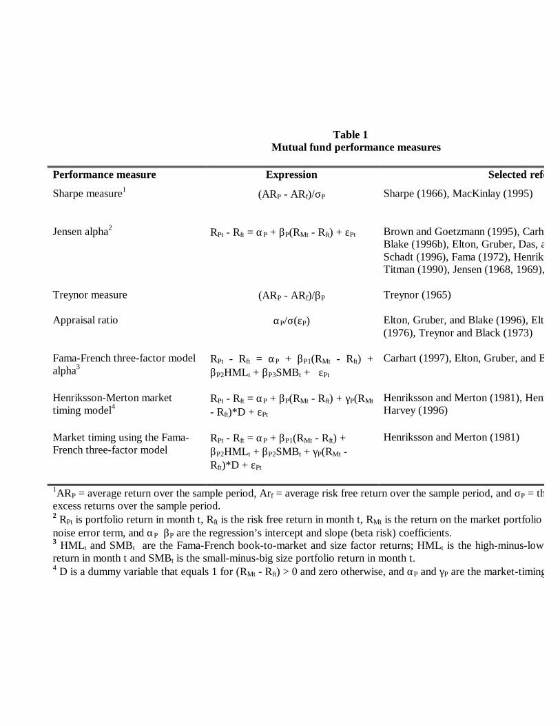
Table 1Mutual fund performance measures

Performance measure Expression Selected references

Sharpe measure1 (ARP - ARf)/σP Sharpe (1966), MacKinlay (1995)

Jensen alpha2 RPt - Rft = αP + βP(RMt - Rft) + εPt Brown and Goetzmann (1995), Carhart (1997), Elton, Gruber, andBlake (1996b), Elton, Gruber, Das, and Hlavka (1993), Ferson andSchadt (1996), Fama (1972), Henriksson (1984), Grinblatt andTitman (1990), Jensen (1968, 1969), Malkiel (1995)

Treynor measure (ARP - ARf)/βP Treynor (1965)

Appraisal ratio αP/σ(εP) Elton, Gruber, and Blake (1996), Elton, Gruber, and Padberg(1976), Treynor and Black (1973)

Fama-French three-factor modelalpha3

RPt - Rft = αP + βP1(RMt - Rft) +βP2HMLt + βP3SMBt + εPt

Carhart (1997), Elton, Gruber, and Blake (1996a)

Henriksson-Merton markettiming model4

RPt - Rft = αP + βP(RMt - Rft) + γP(RMt

- Rft)*D + εPt

Henriksson and Merton (1981), Henriksson (1984), Graham andHarvey (1996)

Market timing using the Fama-French three-factor model

RPt - Rft = αP + βP1(RMt - Rft) +βP2HMLt + βP2SMBt + γP(RMt -Rft)*D + εPt

Henriksson and Merton (1981)

1ARP = average return over the sample period, Arf = average risk free return over the sample period, and σP = the standard deviation ofexcess returns over the sample period.2 RPt is portfolio return in month t, Rft is the risk free return in month t, RMt is the return on the market portfolio in month t, noise error term, and αP βP are the regression’s intercept and slope (beta risk) coefficients.3 HMLt and SMBt are the Fama-French book-to-market and size factor returns; HMLt is the high-minus-low book-to-market portfolioreturn in month t and SMBt is the small-minus-big size portfolio return in month t.4 D is a dummy variable that equals 1 for (RMt - Rft) > 0 and zero otherwise, and αP and γP are the market-timing alpha and gamma.

31Table 2

Distributional properties of 336 regression-based mutual fund performance measures of portfoliosof randomly-selected securities

Sample: Each month from January 1964 through December 1991 (336 months) a 50-stock mutual fund portfolio isconstructed. Its performance is tracked for a three-year period (months 1 through 36). The portfolio composition is changed100% in months 13 and 25. The 50 stocks are selected randomly and without replacement from all NYSE/AMEX stocks withnon-missing return data in month 1, and this procedure is repeated in months 13 and 25 using stocks available in those months.For each of the 336 portfolios, a time-series of monthly returns from month 1 through 36 is constructed. Portfolios returns areequal-weighted at the beginning of months 1, 13, and 25, but they are not rebalanced in the intervening periods. Returns areinclusive of dividends.All the performance measures are as defined in table 1. Performance measures in panel A (B) are estimated using the CRSPvalue-weighted (equal-weighted) index return as the market-factor proxy.Standard errors, S.E., are calculated by applying the Newey-West (1987) correction for serial dependence up to five lags.T-statistics are ratios of the performance measures’ mean values to the standard errors, S.E.Descriptive statistics in panel C are for a sample of 336 three-year average returns on the simulated mutual fund portfolios andCRSP equal- and value-weighted indexes.

Performance measure Mean S.E. t-stat Std.Dev.

Min Median Max Skewness Kurtosis

Panel A: Portfolios of 50 randomly-selected securities, CRSP value-weighted index as market factor

Jensen α in % 0.27 0.088 3.08 0.72 -1.28 0.24 2.69 0.32 2.72

FF 3-factor α in % -0.10 0.022 -4.68 0.35 -1.57 -0.12 1.01 0.14 4.24

CAPM timing α in % 0.63 0.127 4.95 1.07 -2.09 0.60 3.76 0.07 2.51

CAPM timing γ -0.22 0.053 -4.19 0.47 -1.47 -0.30 1.39 0.26 3.18

FF 3-factor timing α in % -0.07 0.043 -1.70 0.59 -2.10 -0.09 2.13 0.22 3.82

FF 3-factor timing γ -0.03 0.019 -1.48 0.29 -0.95 -0.03 1.14 -0.01 3.68

Panel B: Portfolios of 50 randomly-selected securities, CRSP equal-weighted index as market factor

Jensen α in % -0.01 0.019 -0.74 0.31 -0.97 -0.05 1.12 0.47 3.83

FF 3-factor α in % 0.00 0.020 0.00 0.34 -1.10 -0.03 1.03 0.40 3.64

CAPM timing α in % 0.19 0.030 6.17 0.50 -1.25 0.15 1.75 0.27 2.91

CAPM timing γ -0.10 0.015 -6.47 0.21 -0.84 -0.10 0.49 -0.26 3.63

FF 3-factor timing α in % 0.16 0.031 5.00 0.53 -1.64 0.15 1.92 0.04 3.16

FF 3-factor timing γ -0.08 0.014 -5.66 0.21 -0.71 -0.08 0.48 -0.19 3.39

Panel C: Descriptive statistics on returns

Random stocks portfolioreturn %

1.24 0.122 10.14 0.98 -1.49 1.28 3.87 -0.34 2.79

CRSP v-wt return % 0.93 0.073 12.74 0.57 -0.98 0.95 2.40 -0.53 3.58

CRSP eq-wt return % 1.26 0.122 10.29 0.94 -1.66 1.27 3.21 -0.54 2.79

32Table 2 (Cont’d)

The 95th and 99th percentiles of skewness coefficients for a sample of 300 are 0.230 and 0.329, and forsamples of 350 they are 0.213 and 0.305.

Selected percentiles for the kurtosis coefficient are:Sample 1% 5% 95% 99%

300 2.46 2.59 3.47 3.79350 2.50 2.62 3.44 3.72

Table 3Test statistics and rejection frequencies for the regression-based mutual fund performance measures:

Randomly-selected stock portfolios

Sample: Each month from January 1964 through December 1991 (336 months) a 50-stock mutual fund portfolio is constructed. Its performance is tracked for a three-yearperiod (months 1 through 36). The portfolio composition is changed 100% in months 13 and 25. The 50 stocks are selected randomly and without replacement from allNYSE/AMEX stocks with non-missing return data in month 1, and this procedure is repeated in months 13 and 25 using stocks available in those months. For each of the336 portfolios, a time-series of monthly returns from month 1 through 36 is constructed. Portfolios returns are equal-weighted at the beginning of months 1, 13, and 25, butthey are not rebalanced in the intervening periods. Returns are inclusive of dividends.All the performance measures regressions are as described in table 1. Performance measures in panel A (B) are estimated using the CRSP value-weighted (equal-weighted)index return as the market-factor proxy.Distributional properties of the test statistics are for samples of 336 t-statistics from the performance measure regressions described in table 1.Rejection frequencies are based on one-sided tests of the null hypothesis of zero value of the performance measure. The table values report the percentage of times out of336 the null hypothesis is rejected at the specified level of significance.

Distributional properties of test-statistics Rejection frequencies

Performance measure Mean Std.Dev.

Min Median Max Skewness Kurtosis <0.5% <2.5%

Panel A: Portfolios of 50 randomly-selected securities, CRSP value-weighted index as market factor

Jensen α 0.43 1.42 -2.97 0.43 4.30 0.01 2.36 0.6 3.9

FF 3-factor α -0.36 1.02 -3.19 -0.39 3.10 0.13 3.18 1.2 4.5

CAPM timing α 0.82 1.34 -2.20 0.79 4.02 0.05 2.27 0.0 0.3

CAPM timing γ -0.71 1.26 -4.01 -0.75 2.91 -0.07 2.57 4.5 15.5

FF 3-factor timing α -0.16 1.06 -3.22 -0.19 2.96 0.20 2.97 0.6 2.7

FF 3-factor timing γ -0.09 1.13 -3.12 -0.13 3.23 0.05 2.85 0.6 5.1

Table 3 (Cont’d)Panel B: Portfolios of 50 randomly-selected securities, CRSP equal-weighted index as market factor

Jensen α -0.10 1.01 -2.59 -0.18 3.07 0.20 2.90 0.0 2.1

FF 3-factor α -0.04 1.05 -2.90 -0.09 3.33 0.22 2.99 0.3 2.1

CAPM timing α 0.38 1.07 -2.12 0.35 3.64 0.23 2.83 0.0 0.6

CAPM timing γ -0.58 1.16 -4.75 -0.58 2.44 -0.13 3.24 3.0 9.5

FF 3-factor timing α 0.32 1.09 -2.74 0.28 3.79 0.15 2.99 0.3 0.9

FF 3-factor timing γ -0.47 1.16 -4.37 -0.49 2.56 -0.26 3.22 3.0 9.5

35

Table 4Distributional properties of reward-risk ratios of portfolios of randomly-selected securities

Sample: Each month from January 1964 through December 1991 (336 months) a 50-stock mutual fund portfolio isconstructed. Its performance is tracked for a three-year period (months 1 through 36). The portfolio composition is changed100% in months 13 and 25. The 50 stocks are selected randomly and without replacement from all NYSE/AMEX stocks withnon-missing return data in month 1, and this procedure is repeated in months 13 and 25 using stocks available in those months.For each of the 336 portfolios, a time-series of monthly returns from month 1 through 36 is constructed. Portfolios returns areequal-weighted at the beginning of months 1, 13, and 25, but they are not rebalanced in the intervening periods. Returns areinclusive of dividends.All the reward-risk ratios are as described in table 1.Standard errors, S.E., are calculated by applying the Newey-West (1987) correction for serial dependence up to five lags.T-statistics are ratios of the performance measures’ mean values to the standard errors, S.E.Descriptive statistics in panels A and C are for samples of 336 three-year average returns on the CRSP equal- and value-weighted indexes.

Performance measure Mean S.E. t-stat Std.dev.

Min Median Max Skewness Kurtosis

Panel A: CRSP value-weighted index

Sharpe ratio 0.10 0.020 5.05 0.12 -0.33 0.12 0.43 -0.43 3.66

Panel B: Portfolios of 50 randomly-selected securities, CRSP value-weighted index as market factor

Sharpe ratio 0.13 0.020 6.50 0.16 -0.30 0.13 0.55 -0.11 2.70

Treynor measure 0.63 0.099 6.32 0.81 -1.65 0.70 3.13 -0.26 3.01

Appraisal ratio 0.07 0.030 2.47 0.24 -0.51 0.07 0.73 0.01 2.36

Panel C: CRSP equal-weighted index

Sharpe ratio 0.14 0.021 6.71 0.16 -0.32 0.14 0.50 -0.23 2.45

Panel D: Portfolios of 50 randomly-selected securities, CRSP equal-weighted index as market factor

Treynor measure 0.72 0.122 5.87 0.99 -2.12 0.76 3.16 -0.33 3.09

Appraisal ratio -0.02 0.010 -1.60 0.18 -0.45 -0.03 0.52 0.20 2.88

36

Table 5Distributional properties of mutual fund performance measures: Sub-period analysis using

portfolios of randomly-selected securities

Sample: Each month from January 1964 through December 1991 (336 months) a 50-stock mutual fund portfolio isconstructed. Its performance is tracked for a three-year period (months 1 through 36). The portfolio composition is changed100% in months 13 and 25. The 50 stocks are selected randomly and without replacement from all NYSE/AMEX stocks withnon-missing return data in month 1, and this procedure is repeated in months 13 and 25 using stocks available in those months.For each of the 336 portfolios, a time-series of monthly returns from month 1 through 36 is constructed. Portfolios returns areequal-weighted at the beginning of months 1, 13, and 25, but they are not rebalanced in the intervening periods. Returns areinclusive of dividends.Results for subperiod 1964-71 are based on samples of 96 three-year performance measures. Results for subperiods 1972-81and 1982-91 are each based on samples of 120 performance measures.All the regression-based performance measures and reward-risk ratio performance measures are as defined in table 1.Performance measures in panel A (B) are estimated using the CRSP value-weighted (equal-weighted) index return as themarket-factor proxy.Standard errors, S.E., are calculated by applying the Newey-West (1987) correction for serial dependence up to five lags.T-statistics are ratios of the performance measures’ mean values to the standard errors, S.E.Descriptive statistics in panel C are for samples of 96 (subperiod 1964-71), 120 (subperiod 1972-81), and 120 (subperiod 1982-91) three-year average returns on the simulated mutual fund portfolios and CRSP equal- and value-weighted indexes.

Performance measure 1964-71 1972-81 1982-91

Mean S.E. t-stat Mean S.E. t-stat Mean S.E. t-stat

Panel A: Portfolios of 50 randomly-selected securities, CRSP value-weighted index as market factor

Jensen α in % 0.33 0.182 1.81 0.66 0.075 8.77 -0.16 0.076 -2.11

FF 3-factor α in % 0.01 0.042 0.19 -0.15 0.035 -4.14 -0.15 0.024 -6.29

CAPM timing α in % 0.29 0.235 1.23 1.07 0.191 5.60 0.46 0.117 3.93

CAPM timing γ 0.01 0.057 0.18 -0.22 0.100 -2.22 -0.41 0.057 -7.14

FF 3-factor timing α in % 0.28 0.054 5.18 -0.33 0.053 -6.14 -0.10 0.035 -2.93

FF 3-factor timing γ -0.17 0.025 -7.04 0.09 0.023 3.67 -0.03 0.024 -1.12

Treynor measure 0.37 0.183 2.00 0.82 0.144 5.69 0.64 0.111 5.77

Appraisal ratio 0.10 0.056 1.77 0.21 0.025 8.52 -0.09 0.029 -2.93

37

Table 5 (cont’d)Panel B: Portfolios of 50 randomly-selected securities, CRSP equal-weighted index as market factor

Jensen α in % 0.03 0.043 0.77 -0.07 0.027 -2.59 0.00 0.022 0.18

FF 3-factor α in % 0.04 0.041 1.00 -0.03 0.029 -0.86 -0.01 0.027 -0.30

CAPM timing α in % 0.21 0.047 4.10 0.10 0.047 2.06 0.25 0.050 5.00

CAPM timing γ -0.08 0.014 -5.50 -0.06 0.015 -4.20 -0.15 0.031 -4.74

FF 3-factor timing α in % 0.19 0.053 3.64 0.07 0.056 1.19 0.21 0.041 5.23

FF 3-factor timing γ -0.07 0.016 -4.23 -0.04 0.017 -2.24 -0.13 0.023 -5.67

Treynor measure 0.51 0.251 2.02 0.82 0.144 5.69 0.64 0.105 6.09

Appraisal ratio -0.00 0.023 -0.09 -0.04 0.016 -2.75 0.00 0.013 0.00

Panel C: Descriptive statistics on returns and Sharpe ratios of indexes and random stock portfolio

VW index return in % 0.53 0.088 6.00 0.90 0.110 8.16 1.28 0.100 12.82

EW index return in % 0.88 0.229 3.84 1.68 0.175 9.58 1.13 0.103 10.99

Random stocks portfolioreturn in %

0.93 0.243 3.81 1.61 0.174 9.25 1.11 0.100 11.12

VW index Sharpe ratio 0.04 0.024 1.79 0.06 0.019 3.16 0.19 0.016 11.81

EW index Sharpe ratio 0.10 0.041 2.37 0.17 0.027 6.44 0.14 0.025 5.68

Random stocks portfolioSharpe ratio

0.10 0.041 2.31 0.16 0.025 6.32 0.13 0.023 5.70

38

Table 6Distributional properties of mutual fund performance measures of non-randomly sampled

portfolios: large and small market capitalization securities

Sample: Each month from January 1964 through December 1991 (336 months) a 50-stock mutual fund portfolio isconstructed. Its performance is tracked for a three-year period (months 1 through 36). The portfolio composition is changed100% in months 13 and 25. In panel A (B) the 50 large (small) stocks are selected randomly and without replacement from allNYSE/AMEX stocks whose market capitalization falls among the largest (smallest) three deciles of stocks ranked each year onJanuary 1 according to the equity market capitalization of all the NYSE stocks. From this universe of large and small stockseach year, any firm with non-missing return data in month 1 is eligible for inclusion. This procedure is repeated in months 13and 25 using large and small stocks available in those months. For each of the 336 portfolios, a time-series of monthly returnsfrom month 1 through 36 is constructed. Portfolios returns are equal-weighted at the beginning of months 1, 13, and 25, butthey are not rebalanced in the intervening periods. Returns are inclusive of dividends.All the distributional properties are based on samples of 336 performance measures.All the regression-based performance measures and reward-risk ratio performance measures are as defined in table 1. Allperformance measures are estimated using the CRSP value-weighted index return as the market-factor proxy.Standard errors, S.E., are calculated by applying the Newey-West (1987) correction for serial dependence up to five lags.T-statistics are ratios of the performance measures’ mean values to the standard errors, S.E.

Performance measure Mean S.E. t-stat Std.Dev.

Min Median Max Skewness Kurtosis

Panel A: Large capitalization securities, CRSP value-weighted index as market factor

Jensen α in % 0.05 0.016 2.88 0.20 -0.56 0.04 0.69 0.13 3.14

FF 3-factor α in % -0.02 0.013 -1.38 0.19 -0.62 -0.02 0.51 -0.16 3.00

CAPM timing α in % 0.01 0.032 0.19 0.36 -1.02 0.01 1.10 0.17 3.27

CAPM timing γ 0.01 0.017 0.65 0.19 -0.65 0.02 0.64 -0.56 4.33

FF 3-factor timing α in % -0.08 0.028 -2.68 0.36 -1.48 -0.08 0.98 0.12 3.78

FF 3-factor timing γ 0.02 0.016 1.25 0.19 -0.76 0.04 0.54 -0.74 4.71

Return in % 0.99 0.078 12.67 0.63 -1.35 1.03 2.36 -0.62 3.90

Sharpe ratio 0.11 0.016 6.75 0.13 -0.37 0.12 0.48 -0.27 3.87

Treynor measure 0.45 0.071 6.39 0.58 -1.73 0.50 1.84 -0.60 3.94

Appraisal ratio 0.04 0.013 2.69 0.17 -0.53 0.04 0.54 -0.03 3.24

39

Table 6 (Cont’d)

Panel B: Small capitalization securities, CRSP value-weighted index as market factor

Jensen α in % 0.50 0.154 3.23 1.21 -1.79 0.53 3.79 0.20 2.19

FF 3-factor α in % -0.17 0.053 -3.21 0.54 -1.76 -0.15 1.17 -0.28 2.82

CAPM timing α in % 1.10 0.207 5.31 1.69 -2.81 1.06 4.91 -0.03 2.12

CAPM timing γ -0.37 0.095 -3.92 0.80 -2.49 -0.46 3.10 0.48 4.29

FF 3-factor timing α in % -0.16 0.102 -1.52 0.99 -3.15 -0.15 2.06 -0.40 2.92

FF 3-factor timing γ -0.02 0.044 -0.39 0.46 -1.20 -0.04 1.71 0.44 3.53

Return in % 1.47 0.184 7.97 1.45 -2.11 1.51 5.32 -0.06 2.37

Sharpe ratio 0.13 0.023 5.48 0.19 -0.30 0.13 0.57 -0.08 2.28

Treynor measure 0.90 0.201 4.46 2.09 -2.60 0.88 30.9 -8.93 128.7

Appraisal ratio 0.08 0.031 2.52 0.24 -0.50 0.10 0.65 2.30 7.46

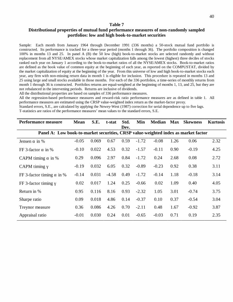
40

Table 7Distributional properties of mutual fund performance measures of non-randomly sampled

portfolios: low and high book-to-market securities

Sample: Each month from January 1964 through December 1991 (336 months) a 50-stock mutual fund portfolio isconstructed. Its performance is tracked for a three-year period (months 1 through 36). The portfolio composition is changed100% in months 13 and 25. In panel A (B) the 50 low (high) book-to-market stocks are selected randomly and withoutreplacement from all NYSE/AMEX stocks whose market capitalization falls among the lowest (highest) three deciles of stocksranked each year on January 1 according to the book-to-market ratios of all the NYSE/AMEX stocks. Book-to-market ratiosare defined as the book value of common equity at the beginning of each year, as reported on the COMPUSTAT, divided bythe market capitalization of equity at the beginning of the year. From this universe of low and high book-to-market stocks eachyear, any firm with non-missing return data in month 1 is eligible for inclusion. This procedure is repeated in months 13 and25 using large and small stocks available in those months. For each of the 336 portfolios, a time-series of monthly returns frommonth 1 through 36 is constructed. Portfolios returns are equal-weighted at the beginning of months 1, 13, and 25, but they arenot rebalanced in the intervening periods. Returns are inclusive of dividends.All the distributional properties are based on samples of 336 performance measures.All the regression-based performance measures and reward-risk ratio performance measures are as defined in table 1. Allperformance measures are estimated using the CRSP value-weighted index return as the market-factor proxy.Standard errors, S.E., are calculated by applying the Newey-West (1987) correction for serial dependence up to five lags.T-statistics are ratios of the performance measures’ mean values to the standard errors, S.E.

Performance measure Mean S.E. t-stat Std.Dev.

Min Median Max Skewness Kurtosis

Panel A: Low book-to-market securities, CRSP value-weighted index as market factor

Jensen α in % -0.05 0.069 0.67 0.59 -1.72 -0.08 1.26 0.06 2.32

FF 3-factor α in % -0.10 0.022 4.53 0.32 -1.57 -0.11 0.90 -0.19 4.25

CAPM timing α in % 0.29 0.096 2.97 0.84 -1.72 0.24 2.68 0.08 2.72

CAPM timing γ -0.19 0.032 6.05 0.32 -0.89 -0.23 0.92 0.38 3.11

FF 3-factor timing α in % -0.14 0.031 -4.58 0.49 -1.72 -0.14 1.18 -0.18 3.14

FF 3-factor timing γ 0.02 0.017 1.24 0.25 -0.66 0.02 1.09 0.40 4.05

Return in % 0.95 0.116 8.16 0.93 -2.32 1.05 3.01 -0.74 3.75

Sharpe ratio 0.09 0.018 4.86 0.14 -0.37 0.10 0.37 -0.54 3.04

Treynor measure 0.36 0.086 4.26 0.70 -2.11 0.48 1.67 -0.92 3.87

Appraisal ratio -0.01 0.030 0.24 0.01 -0.65 -0.03 0.71 0.19 2.35

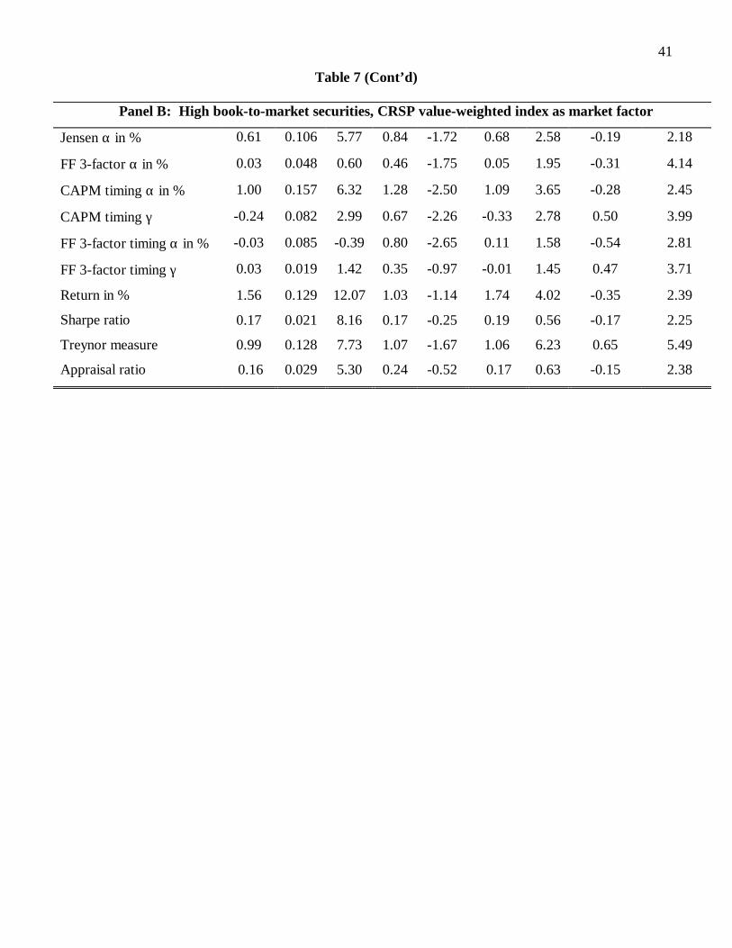
41

Table 7 (Cont’d)

Panel B: High book-to-market securities, CRSP value-weighted index as market factor

Jensen α in % 0.61 0.106 5.77 0.84 -1.72 0.68 2.58 -0.19 2.18

FF 3-factor α in % 0.03 0.048 0.60 0.46 -1.75 0.05 1.95 -0.31 4.14

CAPM timing α in % 1.00 0.157 6.32 1.28 -2.50 1.09 3.65 -0.28 2.45

CAPM timing γ -0.24 0.082 2.99 0.67 -2.26 -0.33 2.78 0.50 3.99

FF 3-factor timing α in % -0.03 0.085 -0.39 0.80 -2.65 0.11 1.58 -0.54 2.81

FF 3-factor timing γ 0.03 0.019 1.42 0.35 -0.97 -0.01 1.45 0.47 3.71

Return in % 1.56 0.129 12.07 1.03 -1.14 1.74 4.02 -0.35 2.39

Sharpe ratio 0.17 0.021 8.16 0.17 -0.25 0.19 0.56 -0.17 2.25

Treynor measure 0.99 0.128 7.73 1.07 -1.67 1.06 6.23 0.65 5.49

Appraisal ratio 0.16 0.029 5.30 0.24 -0.52 0.17 0.63 -0.15 2.38

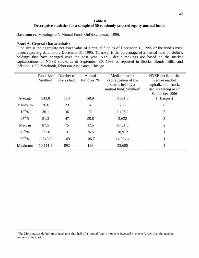
42

Table 8Descriptive statistics for a sample of 50 randomly-selected equity mutual funds

Data source: Morningstar’s Mutual Funds OnDisc, January 1996.

Panel A: General characteristicsFund size is the aggregate net asset value of a mutual fund as of December 31, 1995 or the fund’s mostrecent reporting date before December 31, 1995. Turnover is the percentage of a mutual fund portfolio’sholdings that have changed over the past year. NYSE decile rankings are based on the marketcapitalizations of NYSE stocks as of September 30, 1996 as reported in Stocks, Bonds, Bills, andInflation, 1997 Yearbook, Ibbotson Associates, Chicago.

Fund size,$million

Number ofstocks held

Annualturnover, %

Median marketcapitalization of the

stocks held by amutual fund, $milliona

NYSE decile of themedian market

capitalization stock,decile ranking as of

September 1996Average 543.8 114 58.9 8,001.8 1 (Largest)

Minimum 26.6 23 4 253 8

10th% 30.1 36 20 1,106.2 5

25th% 51.3 47 28.8 2,632 3

Median 87.5 75 47.5 6,421.5 2

75th% 271.6 131 76.5 10,912 1

90th% 1,249.3 169 106.7 14,924.4 1

Maximum 10,111.6 892 196 33,685 1

a The Morningstar definition of median is that half of a mutual fund’s money is invested in stocks larger than the medianmarket-capitalization.

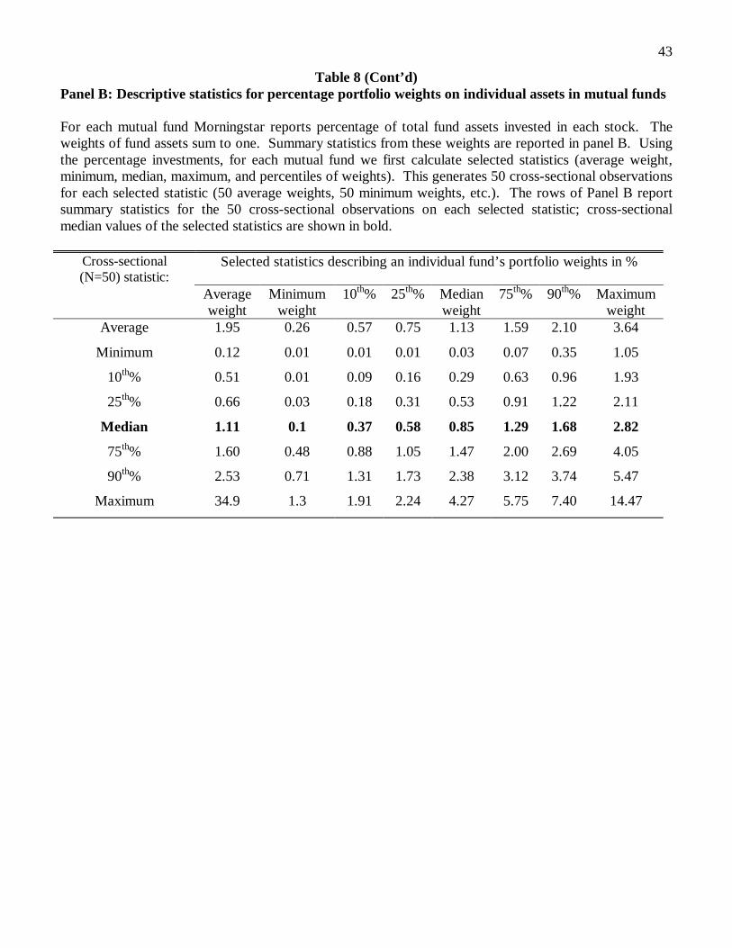
43

Table 8 (Cont’d)Panel B: Descriptive statistics for percentage portfolio weights on individual assets in mutual funds

For each mutual fund Morningstar reports percentage of total fund assets invested in each stock. Theweights of fund assets sum to one. Summary statistics from these weights are reported in panel B. Usingthe percentage investments, for each mutual fund we first calculate selected statistics (average weight,minimum, median, maximum, and percentiles of weights). This generates 50 cross-sectional observationsfor each selected statistic (50 average weights, 50 minimum weights, etc.). The rows of Panel B reportsummary statistics for the 50 cross-sectional observations on each selected statistic; cross-sectionalmedian values of the selected statistics are shown in bold.

Cross-sectional(N=50) statistic:

Selected statistics describing an individual fund’s portfolio weights in %

Averageweight

Minimumweight

10th% 25th% Medianweight

75th% 90th% Maximumweight

Average 1.95 0.26 0.57 0.75 1.13 1.59 2.10 3.64

Minimum 0.12 0.01 0.01 0.01 0.03 0.07 0.35 1.05

10th% 0.51 0.01 0.09 0.16 0.29 0.63 0.96 1.93

25th% 0.66 0.03 0.18 0.31 0.53 0.91 1.22 2.11

Median 1.11 0.1 0.37 0.58 0.85 1.29 1.68 2.82

75th% 1.60 0.48 0.88 1.05 1.47 2.00 2.69 4.05

90th% 2.53 0.71 1.31 1.73 2.38 3.12 3.74 5.47

Maximum 34.9 1.3 1.91 2.24 4.27 5.75 7.40 14.47

Table 9Relation between portfolio performance measures and pre-determined state variables

Performance Measuret,t+3 = g0 + g1 Dividend Yieldt + g2 Book-to-markett + g3 Long-term Government bond yieldDefault premiumt + Errort,t+3

t-statistics are reported below the estimated coefficientsPerformance measures are as described in table 1. All performance measures are estimated using the CRSP value-weighted index return as the market-factor proxy.Dividend yield at the end of month t is the ratio of total dividend in the preceding 12 months on the portfolio of all the NYSE/AMEX stocks to the portfolio’s marketcapitalization at the end of month t.Book-to-market ratio at the end of month t is the value-weighted ratio of the most recent available book-value of common equity of the NYSE/AMEX stocks to themarket capitalization of these stocks at the end of month t.Long-term Government bond yield at the end of month t is the yield-to-maturity on 10-year Government bonds.Term premium at the end of month t is the difference between the long-term Government bond yield and one-month Treasury bill interest rate.Default premium at the end of month t is the difference between the yield on junk bonds and the yield on AAA-rated corporate bonds.

Sample: Each month from January 1964 through December 1991 (336 months) a 50-stock mutual fund portfolio is constructed. Its performance is tracked for a three-year period (months 1 through 36). The portfolio composition is changed 100% in months 13 and 25. For each of the 336 portfolios, a time-series of monthly returnsfrom month 1 through 36 is constructed. Portfolios returns are equal-weighted at the beginning of months 1, 13, and 25, but they are not rebalanced in the interveningperiods. Returns are inclusive of dividends.In panel A, the 50 stocks are selected randomly and without replacement from all NYSE/AMEX stocks with non-missing return data in month 1, and this procedure isrepeated in months 13 and 25 using stocks available in those months.In panel B (C) the 50 large (small) stocks are selected randomly and without replacement from all NYSE/AMEX stocks whose market capitalization falls among thelargest (smallest) three deciles of stocks ranked each year on January 1 according to the equity market capitalization of all the NYSE stocks. From this universe of largeand small stocks each year, any firm with non-missing return data in month 1 is eligible for inclusion. This procedure is repeated in months 13 and 25 using large andsmall stocks available in those months.In panel D (E) the 50 low (high) book-to-market stocks are selected randomly and without replacement from all NYSE/AMEX stocks whose market capitalization fallsamong the lowest (highest) three deciles of stocks ranked each year on January 1 according to the book-to-market ratios of all the NYSE/AMEX stocks. Book-to-market ratios are defined as the book value of common equity at the beginning of each year, as reported on the COMPUSTAT, divided by the market capitalization ofequity at the beginning of the year. From this universe of low and high book-to-market stocks each year, any firm with non-missing return data in month 1 is eligible forinclusion.

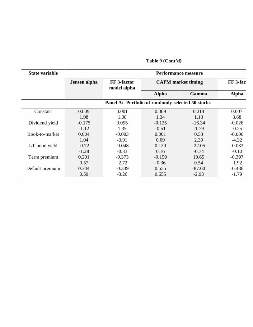
Table 9 (Cont’d)

State variable Performance measure

Jensen alpha FF 3-factormodel alpha

CAPM market timing FF 3-factor market timing

Alpha Gamma Alpha

Panel A: Portfolio of randomly-selected 50 stocks

Constant 0.0091.98

0.0011.08

0.0091.34

0.2141.13

0.0073.68

Dividend yield -0.175-1.12

0.0551.35

-0.125-0.51

-16.34-1.79

-0.026-0.25

Book-to-market 0.0041.04

-0.003-3.91

0.0010.09

0.532.39

-0.006-4.32

LT bond yield -0.72-1.28

-0.048-0.33

0.1290.16

-22.05-0.74

-0.033-0.10

Term premium 0.2010.57

-0.373-2.72

-0.159-0.36

10.650.54

-0.397-1.92

Default premium 0.3440.59

-0.339-3.26

0.5550.655

-87.60-2.93

-0.486-1.79

Table 9 (Cont’d)

Panel B: Portfolio of 50 large stocks

Constant 0.0010.72

-0.000-0.27

-0.000-0.06

0.030.27

0.0010.56

Dividend yield -0.063-1.65

-0.005-0.15

-0.015-0.23

-3.11-1.10

-0.062-1.10

Book-to-market 0.0022.80

-0.001-0.87

-0.000-0.12

0.132.02

-0.000-0.20

LT bond yield 0.0450.38

0.0380.36

-0.002-0.01

5.490.47

0.0310.15

Term premium -0.118-1.19

0.0931.17

-0.105-0.51

2.440.24

0.0810.44

Default premium 0.1861.52

0.1572.11

0.5421.95

-31.09-1.99

0.3161.29

Panel C: Portfolio of 50 small stocks

Constant 0.0010.21

0.0010.28

-0.001-0.15

0.381.14

0.0072.12

Dividend yield 0.2871.38

0.2221.84

0.6452.04

-33.17-1.96

0.3361.99

Book-to-market -0.005-1.06

-0.007-3.18

-0.018-2.42

1.283.27

-0.016-4.99

LT bond yield -0.808-1.04

-0.447-1.27

0.5280.45

-75.27-1.59

0.54-1.09

Term premium 0.5361.60

-0.343-0.96

0.4460.63

-12.95-0.40

-0.505-0.89

Default premium 0.7771.27

-0.389-1.32

0.0960.08

-73.63-1.43

-1.434-2.57

Table 9 (Cont’d)

Panel D: Portfolio of 50 high book-to-market stocks

Constant 0.0143.21

0.0053.03

0.0172.39

-0.16-0.45

0.0082.73

Dividend yield -0.184-1.37

-0.018-0.20

-0.277-1.19

4.120.35

0.0170.13

Book-to-market 0.0051.40

-0.005-3.19

0.0030.55

0.270.88

-0.009-3.03

LT bond yield -0.663-1.24

0.3801.26

0.2540.33

-59.36-1.62

0.4110.94

Term premium 0.2370.62

-0.444-1.51

0.5321.01

-32.12-1.13

-0.395-0.94

Default premium -0.438-0.77

-0.774-3.40

-0.656-0.76

-39.20-0.85

-1.72-4.05

Panel E: Portfolio of 50 low book-to-market stocks

Constant 0.0041.40

-0.000-0.02

-0.001-0.17

0.291.94

0.0042.52

Dividend yield 0.0090.07

0.0631.08

0.2101.12

-15.37-2.51

-0.102-1.62

Book-to-market 0.0021.10

-0.001-0.88

0.0010.15

0.241.45

0.0011.08

LT bond yield -1.051-2.45

-0.362-1.92

-0.56-0.91

-13.29-0.55

-0.179-0.83

Term premium 0.1550.71

0.0060.03

0.1880.54

-3.74-0.21

-0.001-0.01

Default premium -0.387-0.83

-0.200-1.37

-0.734-1.53

-7.67-0.41

-0.465-2.88