Alternative Benchmarks for Evaluating REIT Mutual Fund

Performance∗

Jay C. Hartzell,† Tobias Muhlhofer, and Sheridan TitmanMcCombs School of Business

The University of Texas at Austin

March 15, 2007

∗We would like to thank Crocker Liu and Joe Pagliari for their helpful comments, and Shirley Birmanand Alan Crane for research assistance. We also gratefully acknowledge the financial support of the RealEstate Research Institute. All remaining errors are our own.

†Corresponding author. Department of Finance, McCombs School of Business, The University of Texasat Austin, 1 University Station B6600, Austin, TX, 78712; email: Jay.Hartzell@mccombs.utexas.edu; phone:(512)471-6779; fax: (512)471-5073.

Abstract

While Real Estate Investment Trusts (REITs) have experienced very high growth rates over thepast 15 years, the growth in mutual funds that invest in REITs has been even more dramatic. REITmutual fund returns are typically presented relative to the return on a simple value-weighted REITindex. We ask whether including additional factors when benchmarking funds’ returns can improvethe explanatory power of the models and offer more precise estimates of alpha. We investigate threesets of REIT-based benchmarks, plus an index of homebuilders’ returns. The REIT-based factorsare a set of characteristic factors, a set of property-type factors, and a set of statistical factors.Using traditional single index benchmarks, we find that about six percent of the REIT funds exhibitsignificant positive performance using traditional significance levels, which is more than twice whatrandom chance would predict. However, with the multiple index benchmarks that we prefer, thisfalls by about half, to about three percent. In addition, we find that these sets of factors and thehomebuilders index better explain the month-to-month returns of the REIT mutual funds. Thissuggests that investors or researchers evaluating REIT mutual fund performance may benefit froma multiple benchmark approach.

Keywords: REITs, Mutual Funds, Performance Evaluation

1 Introduction

Over the past several years, the total market value of publicly-traded Real Estate Investment Trusts

(REITs) has grown rapidly. In 1990, prior to the Omnibus Budget Reconciliation Act of 1993 that

changed REIT ownership rules, there were about 117 REITs, with a total market capitalization

of about $8.5 billion. In 1994, after the Act, there were 230 REITs with a combined market

capitalization of about $46 billion. By 2005, while the number of REITs had declined slightly to

208, the total market capitalization had grown to $355 billion, representing a compound annual

growth rate of more than 20%.

Along with this growth in the REIT market has been an even greater growth in mutual funds that

specialize in REITs. Over the same period, the number of REIT funds has grown from 27 to 235,

or more conservatively, the number of unique funds (considering only one share class per fund) has

grown from 16 to 132. Meanwhile, the total market capitalization of all REIT funds has grown at

a compound annual growth rate of nearly 40%, from $1.3 billion in 1994 to $50 billion in 2005.1

This growth has outpaced the overall growth in sector funds, suggesting that real estate funds may

be special among the set of industry-specific investment vehicles.2

Since almost all of these mutual funds are actively managed, there is an interest in evaluating

how funds perform relative to more passive benchmarks. Most REIT mutual funds present their

performance relative to either the NAREIT or the Dow Jones Wilshire indexes, which means that

their goal is to construct a portfolio that is highly correlated with, yet beats, the index. Hence,

at least as a starting point, it makes sense to evaluate how the mutual funds perform relative to

these value-weighted benchmarks. Our null hypothesis is that the mutual funds will not be able to

perform better than these passive benchmarks, which we will test against the alternative that some

of the mutual fund managers have superior information or ability that enable them to generate

returns that outperform these benchmarks.1Note that this total underestimates the total ownership of REITs by real estate-specific asset managers. For

example, mutual fund managers such as Cohen & Steers also manage separate accounts where they purchase REITsfor clients, such as pension funds and endowments, but these do not enter the mutual fund database.

2Tiwari and Vijh (2004) find 308 unique, non-real estate sector funds as of 1999, with a total market value of $151billion, and this was largely driven by 66 technology funds that were worth $72 billion at that time.

1

Since Roll (1978) researchers have been concerned about the specification of the benchmarks used to

evaluate mutual funds. Specifically, the concern is that if inefficient benchmarks are used, passive

portfolios will exhibit evidence of abnormal performance. When this is the case, mutual fund

managers with no special information or abilities can exhibit what looks like positive performance

using these same passive strategies. Our analysis of various REIT portfolios suggests that is indeed

the case when traditional benchmarks are used to evaluate mutual fund managers. In particular,

REIT funds could have outperformed the NAREIT or the Dow Jones Wilshire indexes by simply

concentrating their holdings in smaller capitalization REITs, overweighting industrial REITs, and

by including homebuilding stocks in their portfolios. Morever, our analysis suggests that in the

1994 to 2005 period, a number of REIT mutual funds did in fact follow one or more of these

strategies. Hence, to evaluate the extent to which REIT mutual fund managers have superior

selection skills, one needs to consider benchmarks that account for these systematic deviations

from the value-weighted benchmarks.

Along these lines, we consider three multi-factor benchmarks that are composed of REITs. The first

benchmark consists of the returns to size and book-to-market characteristic-based factors that are

constructed along the lines of the Fama and French (1993) factors, but where the factor returns are

from REITs rather than the broader stock market. The second benchmark consists of the returns

of portfolios sorted by property type. The third benchmark combines these two and consists of the

returns of a set of 13 statistical factor portfolios formed from a factor analysis of a large number of

REIT portfolios based on firm size, book-to-market ratio, and property type. In addition to these

variables, because REIT mutual funds sometimes invest in non-REIT real estate companies, we

consider whether an index of homebuilders’ stock returns adds explanatory power.

Our analysis indicates that a value-weighted portfolio of all REIT mutual funds fails to outperform

any of our alternative benchmarks net of fees. When we add back fees, we find only weak evidence

of average abnormal performance, which is generally not robust to our additional benchmarks.

Although the R square of the single index model is quite high for this value weighted mutual

fund portfolio, at 0.977, additional factors do add significantly more explanatory power. Notably,

our index of homebuilders’ returns is statistically significant in all specifications, suggesting that

2

controlling for the performance of real estate firms other than REITs is important.

To evaluate the importance of the benchmark choice for individual mutual funds, we consider

two dimensions. The first is the extent to which the benchmarks explain the monthly returns of

the funds, i.e., the R square of the regression of the fund returns on the benchmark portfolios.

The general idea is that the benchmark that best explains the monthly returns provides the most

reliable indicator of abnormal return. We then evaluate abnormal return as the intercept from the

regression of the mutual funds’ excess return (over the risk-free rate) on the excess returns of the

benchmark portfolios.

Several interesting facts emerge from this analysis. First, consistent with the results on the value-

weighted portfolio of all funds, adding an index of homebuilders’ returns to any set of benchmark

returns increases explanatory power, especially in the left tail of the distribution of R squares. In

addition, adding homebuilders’ returns generally reduces funds’ estimated abnormal performance,

consistent with some funds earning positive abnormal returns relative to REIT-only benchmarks

by investing in non-REIT stocks.

We also note that the characteristic-based factors and statistical factors appear to perform better

than the property type factors. The property type factors explain less of the variation in returns of

the typical fund, are not quite as good in explaining the left tail of the distribution, and produce

higher estimated alphas. Both the characteristic and statistical factors allow for return differences

due to firm size, while the property type factors do not. Taken together, these results are consistent

with the ability to better explain REIT fund performance by controlling for the positive abnormal

returns to smaller REITs and homebuilders that we observe using our passive portfolios.

Although our analysis suggests that the benchmark choice has only a modest effect on the measured

performance of the value-weighted portfolio of REIT mutual funds, the performance of individual

mutual funds can be much more sensitive to the benchmark choice. Based on the traditional single

index model, we find that 6.16% of funds have a positive alpha net of fees with p-values less than

0.05 (based on a two-tailed test), versus the 2.5% one would expect by chance. However, using the

homebuilders index with either our characteristic or statistical factors reduces this percentage by

3

about half, to 3.42%. When we consider returns before fees, we find that 26.43% of funds have

positive alphas with p-values less than 0.05, but this falls to 15% using our characteristic factors

plus the homebuilders index.

To further understand differences in alphas across different benchmarks, when we examine pairwise

rank correlations of the alphas from our various alternative benchmark models, we find that 14 of

the 28 correlations are less than 0.80, and the lowest is 0.62. In addition, there are some examples

of individual funds that have positive and statistically significant alphas under the single REIT

index model, but negative alphas using the index plus a set of statistical factors. In one extreme

case, for the CGM Realty Fund, the single index monthly alpha is 63 basis points before fees (t

statistic of 2.06), apparently consistent with stock-picking ability. But, the monthly alpha based

on the index plus characteristic factors and our homebuilder index is −5 basis points (t statistic of

−0.19), which does not suggest any abnormal performance, even before fees.

Finally, we examine the relations between fund performance and fund characteristics. Using Fama-

MacBeth (1973) regressions of returns on characteristics, we find little evidence that fund charac-

teristics are systematically related to performance. But, we do find some indication that the more

actively managed funds experienced better performance, and that expense ratios are negatively

related to net-of-fees returns. This latter finding is inconsistent with funds earning their fees back

via superior stock-picking performance.

Our study is most closely related to the analysis of Kallberg, Liu, and Trzcinka (2000), which

studies the performance of 44 REIT mutual funds over the 1986 to 1998 period. In contrast to our

results, they find evidence consistent with significant average abnormal performance (net of fees),

which they attribute to better performance in down markets.3 This difference in overall sector

performance suggests that the drastic growth in the sector may have diluted average fund perfor-

mance.4 They also evaluate several single-index REIT benchmarks, and four-factor benchmarks3Lin and Yung (2004) also study real estate fund performance, but they conclude that there is no evidence of

average abnormal performance over their 1993-2001 sample. Like Kallberg et al., they consider broad stock marketfactors in addition to a REIT index, and conclude that the stock market factors do not materially impact inferenceabout real estate fund performance.

4We obtain qualitatively similar results to Kallberg et al. (2000) when we estimate the alpha on the value-weightedportfolios of all funds over their earlier 1986-1998 time period. Similar to their results, we find some evidence of asignificant positive abnormal return using the Dow Jones Wilshire REIT index (at the 0.10 level), but that significance

4

based on the broader stock market. They find little difference across different REIT indices, and

little explanatory power from the factors based on the overall stock market. They conclude that,

“a real estate index is the appropriate benchmark for evaluating real estate mutual funds” (page

298). Consistent with our results, they find that more actively managed funds experienced better

performance; they also find that larger funds have significantly better performance.

Our study is also related to the large literature on mutual fund performance, which we do not

fully review here. The question of whether mutual funds exhibit abnormal performance, and

the degree to which abnormal performance persists has been studied by many, including Jensen

(1968, 1969), Brown and Goetzmann (1995), Gruber (1996), and Carhart (1997). The use of

appropriate benchmarking is central to this question. The broader mutual fund study that is most

directly relevant to ours is Grinblatt and Titman (1994), who conclude that inference about fund

performance can be strongly influence by the choice of benchmark.

The remainder of the paper is organized as follows. The next section describes our data, including

estimates of performance of passive portfolios formed on firm characteristics. Section three discusses

the ways in which we construct our various alternative benchmarks and presents the empirical

results for alternative benchmark models. Section four discusses the relations between performance

and fund characteristics. Section five concludes.

2 Data

We construct our dataset using the Center for Research in Security Prices (CRSP) Survivorship-

Bias Free U.S. Mutual Fund database. We include all funds that list their detailed objective as

“Equity USA Real Estate,” and collect monthly returns and fund information for the 1994 through

2005 period. In several of our tests, we present our results for “unique” funds only. For this subset,

we collapse multiple share classes into one fund.5 We also collect monthly returns for all U.S. equity

is reduced when we use the NAREIT index. Of note, our characteristic factors are still significant over that timeperiod, beyond the NAREIT index, suggesting that firm size and/or book-to-market were important in that period,as well, and that using the NAREIT index does not completely control for these effects.

5The algorithm we use for reducing the set of funds is as follows. We consider funds of the same family to beduplicates if the R square of a regression of one return on the other is greater than 0.999. If they are duplicates, we

5

REITs, obtained from CRSP, using securities with the second share class digit of eight.

Table 1 presents summary statistics for the mutual funds and REITs over our sample period. The

table documents the rapid growth in the REIT mutual fund industry from 27 funds in 1994 (16 of

which are unique), to 123 funds in 1999 (103 unique), to 235 in 2005 (132 unique). Over this period,

the number or REITs actually declines somewhat, from 230 to 208, but the market capitalization

of REITs grows to nearly eight times its starting level, from $45.9 billion in 1994, to $129.4 billion

in 1999, to $355 billion in 2005. The market capitalization of the mutual funds grows even more

dramatically (almost 38 times), from $1.3 billion in 1994, to $7.4 billion in 1999, to almost $50

billion in 2005. As a result, the fraction of the REIT sector held by REIT-specific mutual funds

has grown over the 11-year period, from about three percent to over 14 percent.

2.1 Single Index Benchmarks

Our starting point for benchmarking fund returns is the Dow Jones Wilshire REIT index, which

is a value-weighted index of REIT returns. We considered both the FTSE NAREIT index and the

Dow Jones Wilshire REIT index, which were the two most commonly cited benchmarks in a hand-

checked subsample of our funds’ annual reports.6 We present results for the Dow Jones Wilshire

REIT index for our analysis because it has the highest explanatory power with respect to the funds’

returns. We simply call this the “Index” for expositional ease. To calculate excess returns on either

our funds, benchmarks, or REITs, we subtract the 30-day Treasury Bill return, as reported by the

St. Louis Federal Reserve. We will later consider multi-factor benchmarks that consist of portfolios

that are formed based on property types, REIT size, and book to market characteristics.

first select the class that is present at a given date if there is only one. Next, we select the retail class based on theCRSP retail indicator if there is one. Then, we select the lowest-fee fund if there is one. If the funds are the samealong all these dimensions, we randomly break the tie.

6As an example, consider the 2006 annual report for the Morgan Stanley Real Estate Fund, available athttp://sec.gov/Archives/edgar/data/1074111/000110465907008604/a06-26022 1ncsr.htm. The report notes, “Mor-gan Stanley Real Estate Fund outperformed both the FTSE NAREIT Equity REIT Index and the Lipper RealEstate Funds Index for the 12 months ended November 30, 2006, assuming no deduction of applicable sales charges.The Fund’s outperformance during the period was driven primarily by bottom-up stock selection, and top-downsector allocation was also favorable. The Fund’s stock selection was especially strong in the mall and office sectors.Within the mall sector, the Fund benefited from its underweight to two of the weakest malls stocks relative to theFTSE NAREIT Equity REIT Index, which had company-specific issues.”

6

2.2 The Performance of Passive Portfolios

Before examining REIT mutual funds we examine whether a variety of passive REIT and home-

builder portfolios can generate abnormal performance relative to the REIT Index over our sample

period. If so, then an active portfolio that has exposure to the passive factors that generate excess

returns will also generate alpha with respect to a single index model.

To assess the performance of such passive strategies, we estimate the performance of characteristic-

sorted portfolios that are based on the market capitalization, the book-to-market ratio, and the

property types of the REITs. Specifically, we form five size and five book-to-market portfolios by

sorting the REITs into the appropriate quintiles. We also construct passive portfolios based on

the five main REIT property types (Hotel, Industrial, Office, Residential, and Retail). Finally, we

include our portfolio of homebuilders.

For each of these portfolios, we calculate the value-weighted monthly returns in excess of the risk-

free rate and regress these excess returns on the excess returns on the Index. The results of these

16 regressions are reported in Table 2. As the table shows, we find strong evidence of a size effect in

our sample. Relative to the Dow Jones Wilshire benchmark, the smallest two quintiles experienced

significant positive alphas, while the largest quintile has a significant negative alpha. The strongest

significance is for the smallest REIT quintile, at 88 basis points per month. This implies that by

overweighting smaller REITs in favor of larger ones, a fund manager could have generated positive

alpha with respect to a single index benchmark over our 11-year period.

In addition, we find positive abnormal returns for three types of real estate firms. Within the

REIT sector, both industrial and retail REITs outperformed the Index, with similar economic

and statistical significance. Both of these groups’ alphas are about 30 basis points per month. Our

index of homebuilders also exhibited strong, significant performance, at 110 basis points per month.

Notably, this portfolio has a low R square with respect to the index at 0.21 (the only lower one

among this set is the smallest set of REITs, at 0.20).

7

3 Evaluating REIT Mutual Fund Benchmarks

The message from Table 2 is that simple passive investment strategies exhibit significant abnor-

mal returns with respect to the single index benchmark over our sample period. This calls for

investigating multi-dimensional benchmarks, which we do in our subsequent tests.

3.1 Characteristic Factors

Our first set of candidate benchmarks consists of REIT-based versions of the size and book-to-

market factors of Fama and French (1993). To construct these, we sort firms into terciles based

on both size (market capitalization) and book-to-market ratio. We then compute HML as the

value-weighted return to the high book-to-market tercile, less the value-weighted return to the low

book-to-market tercile. SMB is defined analogously, as the value-weighted returns to the smallest

firms’ tercile, less the value-weighted returns to the largest firms’ tercile. It is worth noting that this

approach differs from that used previously in studies examining real estate funds’ returns, such as

Kallberg, Liu, and Trzcinka (2000) and Lin and Yung (2004), which use the standard Fama-French

factors for the overall U.S. stock market (which are constructed excluding REITs).

3.2 Property Type Factors

Our next set of candidate benchmark returns consists of returns to property type portfolios. To

construct these, we use the SNL classification of each REIT’s type to form portfolios of five different

property types: Hotel, Industrial, Office, Residential, and Retail. For each property type, we

calculate monthly value-weighted returns over the sample period, and then subtract the REIT

Index return in each month.7

7While we use SNL’s classification of each REIT’s property focus, one could imagine using data on specific propertyholdings to generate more precise estimates. See Geltner and Kluger (1998) for an example of this approach.

8

3.3 Statistical Factor Analysis Portfolios

In order to construct statistical factor analysis portfolios, we need a balanced panel of REIT

portfolio returns. We build one by forming portfolios based on the property types of the assets held

by the REITs, their market capitalizations, and their book-to-market ratios. Specifically, we first

assign REITs into one of five property types: Industrial, Office, Residential, Retail, and “Other”

(all other types). We further split each property type portfolio into thirds, by market capitalization

and by book-to-market ratio.

The end result of these assignments is a balanced panel of 45 value-weighted portfolios formed on

property type, firm size, and book-to-market ratio (five property types, times three size portfolios,

times three book-to-market portfolios). From the returns of these portfolios we subtract the return

on the REIT Index, and then estimate via maximum likelihood a set of 13 statistical factors. This

is the smallest number of factors for which we cannot reject the null that the number of factors is

sufficient to explain the variation in the data. Table 3 presents these results in the form of factor

loadings for each of the 45 portfolios for the nine factors. For the remainder of the analysis, we use

the returns to these 13 statistical factor portfolios as candidate benchmark returns for REIT funds.

As the table shows, the first factor explains seven percent of the variation in the data. The

cumulative fraction explained by the first five factors is 30.8 percent, and this reaches 52 percent

by the thirteenth factor. Thus, even starting with a set of 45 portfolios rather than individual

REITs, a relatively large number of factors is required to explain most of the variation in REIT

returns, consistent with differences in returns due to firm size, property types, and book-to-market,

rather than simply a common U.S. real estate factor. Unfortunately, the loadings themselves do

not reveal any obvious patterns.

3.4 Homebuilder Factor

For our final candidate benchmark return, we use a portfolio of homebuilder stocks. We calculate

the value-weighted monthly returns for all firms on CRSP in SIC code 1531 (Operative Builders)

9

and subtract the REIT Index return, which we then label, Homebuilders. We consider multi-factor

benchmarks that include this factor portfolio along with the other benchmark portfolios described

above.

3.5 Using Alternative Benchmarks to Explain Individual REIT Returns

We begin by investigating the degree to which our alternative benchmarks can explain the returns

to individual REITs. Table 4 reports regressions of monthly excess returns for individual REITs on

the excess returns of the REIT Index, and various factor models. In this table, and in subsequent

tables with individual mutual fund returns, we require a minimum of 24 months of returns for a

REIT (or fund) to be included. The results are consistent with the factor analysis in the sense

that individual REITs exhibit a large degree of idiosynchratic variation. For the mean (median)

firm, the Index alone explains only 20 percent (16 percent) of the variation. Among the alternative

additional benchmarks, the statistical factors appear to add the most explanatory power; the mean

and median R square for these factors is about 0.31. Even though our focus is not on the alphas

of individual REITs, it is interesting to note that the typical alphas generated by the single index

models are larger than those calculated by the other models. As we show below, this difference in

estimated alphas also appears at the mutual fund level.

3.6 Using Alternative Benchmarks to Explain Returns to the REIT Fund Sector

We now turn to the question of the ability of these alternative benchmarks to explain the returns

of REIT mutual funds. To do this, we run regressions of the monthly excess return on a value-

weighted portfolio of all of funds on our various single index and multiple factor benchmarks. In

Table 5, we calculate the average return using the actual returns investors in the funds experienced

(i.e., net of fees), while in Table 6, we use returns before fees (i.e., we add them back to the net

returns).

Model 1 in Table 5 presents the results for a regression using only the Dow Jones Wilshire REIT

10

Index. These results indicate that the single factor REIT Index model explains a great deal of

the variation in the value-weighted funds’ returns; the R square in the regression is 0.977. By way

of comparison, Model 2 presents the results for a similar regression using NAREIT as the single

index. This model has a slightly lower R square of about 0.961, so we focus on the Dow Jones

Wilshire REIT Index for the remainder of the analysis. The point estimate of the alpha in this

single index model is very small, at -0.9 basis points per month (for the Dow Jones Wilshire Index),

and is insignificantly different from zero.8 This is in contrast to the results of Kallberg, Liu, and

Trczinka (2000), who find positive abnormal returns for the average REIT fund in their sample.9

This appears sample specific; if we run this same regression over their sample period (1986 to 1998),

we find some evidence of abnormal performance (at the 0.10 level using two-tailed tests), consistent

with their results.10 Kallberg et al. argue that the positive abnormal performance may be due to an

informational advantage possessed by REIT fund managers. The insignificant results in the recent

time period after the explosive growth in funds is consistent with this advantage being reduced over

time, and with the dilution of the average advantage due to the entry of new managers who may

be less skilled in evaluating REITs.

In Model 3, we add Homebuilders to our base model. As the results indicate, homebuilder returns

have significant incremental explanatory power. The adjusted R square in the regression increases

to 0.982, and the t statistic on Homebuilders is very significant, at 6.49, which is consistent with

REIT fund managers investing in some non-REIT real estate stocks. This is a consistent theme

throughout the table – no matter what set of REIT-based benchmarks is used, Homebuilders is

still significant, and its inclusion increases the model’s adjusted R square. This suggests that8This is inconsistent with the results of Lin and Yung (2004), who find a significant alpha of -46 basis points using

a value-weighted average of real estate mutual funds over the 1997 to 2001 period. They use the NAREIT index, andfind a lower R square than ours, at 0.90 versus our 0.98. They also find no additional explanatory power beyond theNAREIT index for broad stock-market based Fama-French and momentum factors. This suggests that their resultsmay be sample or benchmark specific.

9Our work is also related to previous studies of the performance of institutionally managed real estate investmentsother than mutual funds, such as commingled real estate funds (CREFs). For recent evidence of positive abnormalperformance in a sample of CREFs, see Gallo, Lockwood, and Rodriguez (2006). They use a single-index model toexplain CREF returns, where the index is based on property-level returns, but they also investigate the addition ofregional or property type indexes and find similar results. For prior evidence on CREF performance, see Myer, Webband He (1997), and Myer and Webb (1993).

10Consistent with Kallberg, Liu and Trczinka (2000), we find lower, insignificant alphas when we use the NAREITindex instead of the Dow Jones Wilshire Index. It is worth noting however, that our characteristic factors are stillstatistically significant in their time period using NAREIT as the market index, even though NAREIT includessmaller REITs than the Dow Jones Wilshire Index.

11

benchmarking these funds’ returns can be improved by including such a non-REIT proxy.

In Models 4, 6, and 8, we successively consider adding our characteristic factors, property type

factors, and statistical factors to the single index. Models 5, 7, and 9 present identical specifica-

tions, respectively, except for the addition of Homebuilders. The property type regressions offer

the highest adjusted R squares (0.980 without Homebuilders), although all of the alternatives im-

prove the explanatory power relative to the single index model (adjusted R squares of 0.978 for the

characteristic factors and 0.979 for the statistical factors, respectively). F-statistics for tests of the

joint hypothesis that all of the coefficients except for that on the Index (and Homebuilders, if it is

included) are zero, are also the highest for the property type factors, although they are also signif-

icant in the statistical factor and characteristic factor regressions, without Homebuilders. Across

models, there is no evidence of significant positive abnormal performance. The only significant

alphas are in Models 5 and 9, and their estimates are negative nine and negative eight basis points

per month, respectively.

In Table 6, we present results from identical specifications, except we use the value-weighted excess

return on all of the funds before fees (i.e., we add back fees to the CRSP returns by adding 112 of

the annual expense ratio to each month’s return). As one would expect, the explanatory power of

the various models is virtually unchanged. Of more interest is the estimated abnormal performance

across different specifications. We find significant positive abnormal performance in specifications

using the single indexes (Dow Jones Wilshire or NAREIT), statistical factors and property type

factors. The magnitude of this performance is plausible, at 10 basis points per month (about 1.2

percent per year) for the Dow Jones Wilshire single index model. But, the estimated abnormal

performance is reduced in every alternative by the addition of Homebuilders; the estimated alpha

is not signficant in any model where this is included. In addition, the alpha is insignificant in the

characteristic factor model, although the point estimate is not very different from the single index

model (seven basis points versus 10 basis points per month). Taken together, the results suggest

that the average REIT fund exhibits some abnormal performance, but that the performance is offset

by expenses. They are also consistent with the results of Table 2, which suggest that fund managers

add alpha in this sample by overweighting smaller REITs and buying homebuilders’ stocks.

12

3.7 Using Alternative Benchmarks to Explain Individual REIT Fund Returns

While these results suggest that additional factors beyond a single index can more precisely estimate

abnormal performance for the group of REIT funds as a whole, our ultimate question is whether

these alternative benchmarks provide better assessments of the performance of individual funds. To

address this, we run separate time series regressions of each fund’s excess monthly returns on our

same alternatives (the single index, plus characteristic factors, property type factors, and statistical

factors, with and without Homebuilders). In Table 7, for each of these alternatives, we summarize

the distribution of three key statistics across the sample of funds: the adjusted R square, alpha,

and the t-statistic for the alpha. We also present additional statistics regarding the distribution of

alphas: the cross-sectional standard deviation of estimated alphas, and the percentage of alphas

that are significantly positive and negative. For these significance calculations, we tabulate the

fraction of alphas with p-values that are less than or equal to 0.05, separated by whether they

are positive or negative. Note that since these p-values are based on two-sided tests, random

chance would predict that 2.5% of alphas are significantly positive, with another 2.5% significantly

negative.

First, as one can see from the table, the benchmarks do a very good job of explaining the variation

in returns of the typical fund. The single index model produces a mean (median) R square of 0.903

(0.955). By way of comparison, in their 1986 to 1998 sample, Kallberg, Liu, and Trczinka (2000)

find a mean (median) R square of 0.851 (0.91) with respect to the Wilshire REIT index. This

suggests that typical REIT funds more closely track this index than they did previously.

Benchmarks that more accurately explain monthly returns will produce more precise estimates of

fund performance. In addition to considering the improved explanatory power for a typical fund, we

also consider whether the additional factors increase the R squares of the funds for which the single

index model performs most poorly. In the middle of the distribution, the results are consistent with

what we found for the value-weighted index of all funds. We find that all of the multiple factor

models improve explanatory power beyond the single index; median and mean R square are higher

in all of these alternatives. Based solely on this criterion, the statistical factors with Homebuilders

13

offer the highest mean and median adjusted R square (0.935 and 0.964, respectively). The addition

of Homebuilders also improves explanatory power for the typical fund. For explaining the left-tail

outliers, the statistical factor model with Homebuilders again offers the biggest improvement, with

a 10th percentile adjusted R square of 0.853 versus 0.744 for the single index model.

In addition to improvements in R squares, we also care about estimated alphas and their statistical

significance. The mean (median) monthly alpha using the single index is only about -0.1 (-0.01)

basis points. In contrast, the mean (median) alpha using the same benchmark reported in Kallberg,

Liu, and Trczinka (2000) for their earlier time period is 18 basis points (9 basis points) per month.

This difference across samples is not surprising given our results on the alpha of the value-weighted

portfolio of all funds.

Based on the standard deviations of alphas across different benchmarks, the multiple index models

do not appear to reduce the variation in alphas across funds. While the characteristic factors model

has the lowest standard deviation (0.00178), the single index model’s standard deviation is the next

lowest (0.00182). However, if one looks at reductions in the right tail of estimated alphas, and the

extreme t statistics, the models using statistical factors and characteristic factors with Homebuilders

appear to work well. The 90th percentile of alpha is reduced from 21 basis points per month in the

single index model to 13 basis points for the statistical factors with Homebuilders model, and to

10 basis points in the characteristic factors with Homebuilders model. The t statistic drops from

1.52 to 1.24 or to 1.06, respectively, at the same point in the distribution. At the middle of the

distribution, the estimated alphas from these two alternatives also appear to be more conservative

than the single index. Compared to the average and median alphas based on the single index

model that were basically zero, when one adds the statistical factors and Homebuilders, the mean

(median) alpha is -8 basis points (-7 basis points). Similarly, for the models using the characteristic

factors and Homebuilders, the mean (median) alpha is -11 basis points (-8 basis points). Typical

alphas using the property type factors are higher than those based on the characteristic or statistical

factors when Homebuilders is not included, consistent with an important firm size component of

returns over this sample.

These reductions in right-tail alphas can also be seen by examining the fraction of significant positive

14

alphas across models. For the single index model, 6.16% of alphas are positive and significant at

the 0.05 level (using two-tailed tests), which is more than twice what would be expected based

on random chance. Three alternative models reduce this proportion by almost half, to 3.42%:

the single index model with Homebuilders, the characteristic factors with Homebuilders, and the

statistical factors with Homebuilders. The characteristic factors with Homebuilders produces the

largest fraction with estimated negative significant performance, at 18.49%, versus 10.27% for the

single index model.

Figure 1 presents box-and-whisker plots of the alphas of the single Index model, as well as each

alternative model including Homebuilders. In the figure, the solid middle line represents the me-

dian alpha, while the upper and lower edges of each box represent the first- and third quartiles,

respectively. The dashed vertical lines (the whiskers) extend 1.5 times the interquartile range (the

length of the box) from the edges, while any remaining outliers beyond this distance are plotted

individually as circles. As the figure shows, the Index-only model generates alphas that are notice-

ably higher than any of the alternative models that include the Homebuilders index, both in terms

of the medians and the left tail of the distribution. Among the models that include Homebuilders,

median alphas are slightly smaller using the characteristic or statistical factors. In addition, these

two models result in tighter distributions than the other alternatives.

Table 8 presents the same information as Table 7, but using returns to funds before fees (i.e., with 112

of the annual expense ratio added to each fund’s monthly return). Since fees do not vary much with

the factors, we find little difference in explanatory power. Of more interest are the estimated alphas.

Here, again, the combinations of the characteristic or statistical factors and Homebuilders appear

to offer the most conservative approaches. For example, using the single index, the 75th percentile

of the alpha distribution is 20 basis points per month, while the t statistic at that percentile is 2.03.

In contrast, using characteristic factors plus Homebuilders, the 75th percentile alpha and t-statistic

are 16 basis points and 1.62, respectively. For the statistical factors plus Homebuilders, we also see

a reduction in estimated abnormal performance, although not quite as large. The estimated alpha

and t-statistic at those same cutoffs are 17 basis points and 1.77, respectively. However, while

looking at the percentage of funds with significantly positive alphas, the statistical factors (plus

15

Homebuilders) is the most conservative. While 26.43% of funds have positive alphas with p-values

of less than or equal to 0.05, this drops to 15% for the statistical factors model with Homebuilders

(compared to 19.29% for the characteristic factors with Homebuilders). The property type factors

plus Homebuilders offers the smallest reduction in alphas, with a 75th percentile estimated alpha

and t-statistic of 22 basis points and 1.89, respectively.

Comparing the results of Tables 7 and 8, we find evidence consistent with a fairly large percentage

of REIT fund managers producing significant alpha before fees. Even using our most conservative

model, our estimates imply that 15% of funds had positive significant alphas, much more than

the 2.5% level one would expect by chance. But, after fees, the incidence of abnormal positive

performance is much more in line with statistical norms, at 3.42% In contrast, the incidence of

negative abnormal performance before fees is in line with random chance (around three percent,

depending on the model used), but after fees, this becomes as high as 18.49%.

While these results help us understand the distribution of alphas across various model choices, they

do not say anything about how the different benchmarks affect estimated alphas for a particular

fund. To assess this, we first check how the top ten funds in terms of performance using the single

index model faired against our multiple benchmark models. In Table 9, we present the alphas

across different models that include Homebuilders for the 10 funds with the largest alphas from

the single index model. For all of the funds, the multiple benchmarks produce more conservative

estimates of performance. For example, for the top fund, the Third Avenue Real Estate Fund,

the estimated alpha is 71 basis points per month for the single index model, but this falls to 44

basis points using the characteristic factors with Homebuilders. More generally, for half of this

subsample, including Third Avenue, the benchmark choice does not matter much, but for the other

half, it matters a lot. For five of the 10 funds, the estimated alphas are consistently positive and

of similar maginitude. But, for the other five, alphas are actually negative for the characteristic

factor model with Homebuilders.

To further investigate changes in alpha ranks across models, we calculate the Spearman rank

correlations of the alphas from our eight candidate models (single index, plus characteristic factors,

property type factors, or statistical factors, with or without Homebuilders). These rank correlations

16

are presented in Table 10. Several facts emerge from data. First, the addition of the homebuilders

returns appears to have important effects beyond the single index model. The rank correlation

between the single index model and the single index model with homebuilders is only 0.83, and

this falls to between 0.66 and 0.73 for the other factors plus homebuilders. Second, by looking

at the correlation of alphas between a set of factors without homebuilders and that same set with

homebuilders, it appears that including homebuilders has the biggest impact on the ranks of alphas

of the single index model (rank correlation of 0.83) and the statistical factors (rank correlation of

0.82). Finally, given the performance of the characteristic and statistical factors with Homebuilders

models in the previous tables, it is useful to examine those models’ rank correlations specifically. As

one might expect, the statistical factors plus Homebuilders model appears to capture parts of the

property type and characteristic factors. The rank correlation between the statistical factor model

alphas and either the property type factor alphas or the characteristic factor alphas are higher than

that between the property type and characteristic factors (0.86 and 0.82, versus 0.77).

4 Performance as a Function of Fund Characteristics

We conclude our analysis by investigating the relations between fund performance and various fund

characteristics. While we find no evidence of abnormal performance for a typical fund, it may be

that some fund performance is related to characteristics such as fund size, expenses, and the degree

to which the fund appears to be actively managed. To test for this, we conduct regressions in the

style of Fama-MacBeth (1973). For each year in the sample, we run a cross-sectional regression of

fund returns (net of fees, or with fees added back) on fund characteristics. We then present the

average coefficient and t statistic for each variable across the time series, where the t statistic is

calculated based on the ratio of the average coefficient to the time-series standard deviation of the

coefficient. This technique allows for cross-sectional correlation in performance at any given point

in time, as the statistical significance relies on time series variation.

The characteristics we investigate are firm size (the natural logarithm of the fund’s net asset value

as of the end of the previous year, denoted Ln(Sizet−1)), the total expense ratio (Expenses), the

17

annual fund turnover (as reported on CRSP, denoted Turnover), the total number of holdings

of the fund (Holdings), and an indicator variable for funds with loads (Load). Kallberg et al.

(2000) find evidence consistent with larger funds and more actively managed funds exhibiting

greater performance. If this were true in our sample, we would expect a positive coefficient on

our fund size variable, a positive coefficient on Turnover, and a negative coefficient on Holdings

(as more actively managed funds would hold fewer REITs than the index, and would trade more

aggressively). We are also interested in the coefficients on the Expenses variable across the two

regressions net of fees and with fees added back. If fees are uncorrelated with stock-picking ability,

then we would expect an insignificant coefficient for Expenses in the regression with fees added

back to returns, and a coefficient of -1.0 on expenses in the regression using returns net of fees. In

contrast, if expenses were strictly based on stock-picking ability and passed through to investors

accordingly, we would expect a coefficient of 1.0 in the before-expenses regression, and a coefficient

of zero in the net-of-expenses regression.

The results of these tests are presented in Table 11. Unfortunately, we are unable to explain much

of the variation in returns across our sample, perhaps due to a lack of power given the small number

of years. We do find a significant negative coefficient on expenses in the net-of-fees regression and

an insignificant coefficient in the before-fees regression, which are more consistent with a lack of

correlation between stock picking and expense ratios. There is some marginal evidence of a relation

between active management and performance; the point estimate on Turnover is positive and the

point estimate on Holdings is negative, and the p value on the former is about 0.12 in a two-tailed

test. We find little evidence of relations between performance and fund size or the presence of a

load.

5 Conclusion

REIT mutual funds have experienced a tremendous recent growth in popularity. These funds are

actively managed and charge substantial fees that reflect the possibility that their active manage-

ment will generate returns that exceed the returns that can be generated with passive investment

18

strategies. In order to evaluate whether these funds do in fact generate abnormal returns, we need

benchmark portfolios that allow us to evaluate the marginal benefits of active portfolio manage-

ment. This study examines these indexes and considers some multiple factor benchmarks that can

potentially provide better assessments of the performance of REIT mutual funds.

Our study first documents that over our sample period, simple passive portfolios that concentrated

on smaller REITs, or non-REIT real estate firms (homebuilders) generate significant alphas with

respect to the commonly used single REIT index benchmarks. This suggests that alternative

benchmarks may add explanatory power beyond the index, which should lead to more precise

estimates of abnormal performance. We investigate three sets of REIT-based benchmarks, plus

an index of homebuilders’ returns. The REIT-based factors are a set of statistical factors, a set

of property-type factors, and a set of Fama-French type characteristic factors that are zero-cost

portfolios of REITs.

Our statistical factors and these REIT-based characteristic factors, when combined with home-

builders’ returns and the REIT index, appear to offer the most attractive traits as benchmarks

for fund returns. These models do the best job in improving the explanatory power for the funds

with the lowest R squares based on the Index alone. Furthermore, in terms of estimating alphas,

these models appear more conservative and help explain extreme outliers in terms of positive ab-

normal performance based on the single index. Consistent with the evidence of abnormal returns

of passive portfolios, our results suggest that including benchmarks that are sensitive to firm size,

book-to-market, and non-REIT returns materially affects inference about fund performance.

19

References

[1] Brown, S.J. and W.N. Goetzmann. 1995. Performance Persistence. Journal of Finance 50:

679-698.

[2] Carhart, M. M. 1997. On Persistence in Mutual Fund Performance. Journal of Finance 52:

57-82.

[3] Fama, E.F. and K.R. French. 1993. Common Risk Factors in the Return on Bonds and Stocks.

Journal of Financial Economics 33: 3-53.

[4] Fama, E.F. and J.D. MacBeth. 1973. Risk, Return, and Equilibrium: Empirical Tests. Journal

of Political Economy 81: 607-636.

[5] Gallo, J.G., L.J. Lockwood and M. Rodriguez. 2006. Differentiating CREF Performance. Real

Estate Economics 34: 173-209.

[6] Geltner, D. and B. Kluger. 1998. REIT-Based Pure-Play Portfolios: The Case of Property

Types. Real Estate Economics 26: 581-612.

[7] Grinblatt, M. and S. Titman. 1994. A Study of Monthly Mutual Fund Returns and Performance

Evaluation Techniques. Journal of Financial and Quantitative Analysis 29: 419-444.

[8] Gruber, M.J. 1996. Another Puzzle: The Growth in Actively Managed Mutual Funds. Journal

of Finance 51: 783-810.

[9] Jensen, M. 1968. The Performance of Mutual Funds in the Period 1945-1964. Journal of

Finance 23: 389-416.

[10] Jensen, M. 1969. Risk, the Pricing of Capital Assets, and the Evaluation of Investment Port-

folios. Journal of Business 42: 167-247.

[11] Kallberg, J.G., C.L. Liu and C. Trzcinka. 2000. The Value Added from Investment Managers:

An Examination of Funds of REITs. Journal of Financial and Quantitative Analysis 35: 387-

408.

20

[12] Lin, C.Y. and K. Yung. 2004. Real Estate Mutual Funds: Performance and Persistence. Journal

of Real Estate Research 26(1): 69-93.

[13] Myer, F.C.N. and J.R. Webb. 1993. The Effect of Benchmark Choice on Risk-Adjusted Per-

formance Measures for Commingled Real Estate Funds. Journal of Real Estate Research 8(2):

189-203.

[14] Myer, F.C.N., J.R. Webb and L.T. He. 1997. Issues in Measuring Performance of Commingled

Real Estate Funds. Journal of Real Estate Portfolio Management 3(2): 79-85.

[15] Roll, R. 1978. Ambiguity when Performance is Measured by the Securities Market Line. Journal

of Finance 33: 1051-1069.

[16] Tiwari, A. and A.M. Vijh. 2004. Sector Fund Performance: Analysis of Cash Flow Volatility

and Returns. Working Paper. University of Iowa.

21

Table 1: Summary of the Number and Market Captialization of Mutual Funds and REITs.This table presents the number of mutual funds that specialize in US Equity Real Estate as well as their total market capital-

izations at the end of each year of our sample. Number of Unique Funds represents the number of mutual funds after we join

funds in the same family which seem to hold the same portfolio. As a comparison, we also present for each year the number of

publicly traded REITs and their total market capitalizations.

Year Number Number Fund Number REITof Funds of Unique Funds Market Cap of REITs Market Cap

1994 27 16 1,325 230 45,862

1995 37 37 2,019 231 60,175

1996 54 53 5,710 215 91,069

1997 72 64 11,964 226 138,868

1998 101 90 8,807 228 141,646

1999 123 103 7,436 221 129,404

2000 135 108 11,106 204 145,098

2001 144 107 12,072 197 159,644

2002 134 105 14,974 191 168,193

2003 162 125 25,888 187 235,617

2004 216 128 41,275 204 324,879

2005 235 132 49,967 208 355,046

All market capitalization figures are in millions of U.S. Dollars.

22

Table 2: R squares, Alphas, and T-statistics for Passive Portfolios Formed Using Individual Factors.This table presents R squares, alphas, and t-statistics of alphas from a set of univariate regressions of each individual factor

on the index. The factors used are size quintile portfolios of REITs (numbered from smallest to largest), book-to-market ratio

quintile portfolios (numbered the same way), the portfolio of homebuilders, and the individual property-type portfolios.

R square alpha t-statistic

Size.1 0.1962 0.0088 3.6599∗∗∗

Size.2 0.4787 0.0051 2.1977∗

Size.3 0.7142 0.0025 1.3600

Size.4 0.8667 0.0018 1.4687

Size.5 0.9731 −0.0012 −2.0187∗

BE.ME.1 0.8782 −0.0001 −0.0765

BE.ME.2 0.9165 −0.0008 −0.7620

BE.ME.3 0.8553 0.0010 0.7882

BE.ME.4 0.6268 0.0009 0.3722

BE.ME.5 0.4628 0.0044 1.4642

Homebuilders 0.2139 0.0110 2.0508∗

Hotel 0.4837 −0.0040 −0.9023

Industrial 0.8146 0.0034 2.1805∗

Office 0.8553 0.0012 0.8575

Residential 0.8533 0.0004 0.3284

Retail 0.8239 0.0029 2.0239∗

◦: p < 10%; ∗: p < 5%; ∗∗: p < 1%; ∗∗∗: p < 0.1%.

23

Tab

le3:

Fact

orLoa

ding

sfo

rTri

ple-

Sort

Por

tfol

ios.

This

table

pre

sents

fact

or

loadin

gs

for

stati

stic

alfa

ctors

com

pute

don

port

folios

ofR

EIT

s,so

rted

sim

ult

aneo

usl

yby

pro

per

tyty

pe,

size

,and

book-t

o-m

ark

etra

tio.

The

firs

tpart

ofea

chport

folio

nam

ere

fers

topro

per

tyty

pe,

the

seco

nd

tosi

ze,and

the

thir

dto

book-t

o-m

ark

et.

At

the

bott

om

ofth

eta

ble

,w

ein

dic

ate

for

each

fact

or

Nth

ecu

mula

tive

pro

port

ion

ofth

evari

ance

expla

ined

by

all

fact

ors

n≤

N,as

wel

las

the

valu

eofa

χ2

test

statist

icth

at

the

13

fact

ors

pre

sente

dher

eare

suffi

cien

tin

expla

inin

gth

esy

stem

ati

c

vari

ance

ofth

esy

stem

.

round

Facto

r1Facto

r2Facto

r3Facto

r4Facto

r5Facto

r6Facto

r7Facto

r8Facto

r9Facto

r10

Facto

r11

Facto

r12

Facto

r13

Indust

rial.big

.hig

h0.1

490

−0.4

463

0.1

084

−0.0

547

0.1

261

0.0

620

−0.0

983

0.2

635

−0.1

287

0.0

507

−0.0

315

−0.1

230

−0.1

472

Indust

rial.big

.low

0.1

090

−0.0

040

−0.2

051

−0.1

525

−0.0

120

−0.0

220

0.0

464

−0.1

829

−0.4

066

−0.0

127

−0.1

352

0.0

442

−0.0

070

Indust

rial.big

.med

0.0

112

0.1

413

0.1

439

−0.0

619

0.0

902

0.1

202

−0.0

063

0.4

641

−0.0

648

0.0

371

−0.0

439

0.0

725

0.0

361

Indust

rial.m

id.h

igh

0.0

285

0.1

361

−0.0

420

−0.0

328

0.1

138

0.8

307

0.0

394

0.1

563

0.0

180

0.0

433

0.0

139

0.0

235

0.0

463

Indust

rial.m

id.low

0.0

620

0.0

224

0.2

177

−0.0

003

0.0

148

0.1

754

0.0

673

0.2

026

−0.0

052

0.1

277

0.1

022

0.6

181

−0.0

549

Indust

rial.m

id.m

ed

0.1

028

0.0

894

0.0

111

−0.0

594

0.1

292

0.7

820

−0.1

145

0.1

064

0.0

646

0.0

897

−0.0

943

0.1

631

0.0

192

Indust

rial.sm

all.h

igh

0.1

509

0.8

743

0.0

931

0.0

842

0.1

275

0.0

799

0.0

157

0.1

835

−0.0

318

0.0

015

0.0

046

0.0

360

−0.0

052

Indust

rial.sm

all.low

0.0

887

0.8

202

0.0

214

0.0

738

−0.1

112

0.1

546

0.0

508

0.2

460

−0.0

099

0.0

644

0.0

536

0.0

007

−0.2

641

Indust

rial.sm

all.m

ed

0.1

484

0.9

642

0.0

474

0.0

683

0.1

011

0.0

764

−0.0

405

−0.0

315

0.0

111

0.0

090

−0.0

107

−0.0

424

0.0

489

Offi

ce.b

ig.h

igh

−0.1

617

−0.0

798

0.1

260

0.0

200

−0.6

653

0.0

442

0.3

345

0.1

392

0.0

528

0.0

300

0.0

359

−0.2

080

0.1

045

Offi

ce.b

ig.low

−0.1

029

0.0

251

0.0

084

−0.0

656

−0.0

585

0.1

162

−0.0

195

0.0

487

0.0

100

0.9

759

0.0

148

0.0

570

0.0

622

Offi

ce.b

ig.m

ed

−0.0

214

−0.0

498

0.0

297

−0.0

087

0.0

267

−0.0

829

0.0

479

0.2

541

−0.5

590

−0.0

928

0.0

259

0.0

006

−0.1

030

Offi

ce.m

id.h

igh

0.2

630

0.0

182

−0.0

838

0.0

675

0.0

021

−0.2

931

0.0

940

0.2

929

−0.3

139

0.1

549

0.0

895

−0.4

060

0.0

344

Offi

ce.m

id.low

−0.0

172

−0.0

390

−0.0

451

0.0

576

−0.0

841

0.0

375

0.0

218

−0.0

617

0.0

101

0.0

626

0.0

107

−0.0

508

0.5

599

Offi

ce.m

id.m

ed

0.0

647

0.0

416

0.0

241

0.0

916

−0.1

275

0.0

940

−0.0

006

0.6

437

−0.1

077

0.0

269

−0.0

059

0.0

446

−0.0

734

Offi

ce.s

mall.h

igh

0.0

194

−0.0

053

0.3

094

−0.0

013

0.0

613

0.0

371

−0.0

604

0.1

148

0.0

966

0.0

048

0.1

110

0.1

157

−0.0

262

Offi

ce.s

mall.low

−0.1

061

0.0

881

0.1

531

−0.0

268

0.6

480

0.2

030

−0.0

889

−0.0

123

0.0

241

0.0

136

0.0

650

−0.0

738

−0.0

152

Offi

ce.s

mall.m

ed

0.0

876

−0.1

475

0.0

652

0.0

310

−0.1

311

0.2

210

0.2

021

−0.0

045

−0.2

078

−0.0

156

0.1

503

−0.1

141

0.1

761

Oth

er.

big

.hig

h0.2

299

0.0

901

0.1

494

0.5

554

−0.0

260

−0.0

763

0.0

542

0.0

057

−0.0

440

0.1

376

0.0

519

−0.0

214

−0.0

588

Oth

er.

big

.low

0.0

044

0.1

397

0.1

136

0.0

764

−0.0

188

−0.0

485

0.3

336

−0.1

011

−0.0

268

−0.0

988

0.0

930

0.2

420

−0.1

051

Oth

er.

big

.med

−0.0

354

0.1

347

−0.2

404

0.5

998

0.0

944

−0.0

515

0.1

234

−0.0

574

−0.0

569

−0.1

246

0.0

833

0.0

772

0.0

283

Oth

er.

mid

.hig

h0.1

819

0.0

358

0.2

241

0.6

653

−0.0

405

−0.0

063

0.0

130

0.0

703

0.1

077

−0.0

666

−0.0

198

−0.0

049

0.0

986

Oth

er.

mid

.low

0.4

077

0.0

277

0.1

918

0.2

534

0.0

060

0.0

150

0.2

027

0.2

162

0.0

544

−0.0

581

0.1

666

0.0

500

0.0

200

Oth

er.

mid

.med

0.3

935

−0.0

328

0.1

511

0.4

480

0.0

810

0.0

582

0.3

383

−0.0

020

0.1

153

−0.0

882

0.1

861

−0.1

387

0.1

206

Oth

er.

small.h

igh

0.3

689

0.0

760

0.0

660

−0.0

700

0.1

154

−0.1

014

0.2

865

0.0

068

−0.0

117

−0.0

277

0.4

564

0.0

152

0.0

991

Oth

er.

small.low

0.1

573

−0.0

245

0.3

012

0.2

410

0.0

136

0.0

494

0.3

586

0.0

599

0.0

464

−0.1

163

0.1

332

−0.0

294

0.2

092

Oth

er.

small.m

ed

0.4

349

0.0

562

0.4

633

0.1

793

0.0

449

0.0

268

0.3

704

−0.2

197

−0.0

791

−0.0

684

0.1

123

0.1

664

−0.0

464

Resi

denti

al.big

.hig

h−

0.0

484

−0.0

555

0.1

771

−0.0

551

0.0

766

−0.0

162

−0.5

937

0.0

254

−0.0

286

−0.0

306

−0.0

463

0.0

389

0.0

256

Resi

denti

al.big

.low

−0.1

288

0.0

360

0.1

834

−0.1

788

−0.4

637

0.0

081

−0.2

380

−0.1

650

0.0

390

−0.0

370

−0.0

545

−0.0

151

0.1

222

Resi

denti

al.big

.med

−0.2

953

0.1

056

0.0

351

−0.0

620

−0.1

862

0.3

052

−0.5

318

−0.0

959

0.0

609

−0.0

774

0.1

779

−0.0

749

−0.1

182

Resi

denti

al.m

id.h

igh

0.1

993

0.0

350

0.6

330

0.0

542

−0.0

589

−0.0

068

−0.1

743

0.1

397

−0.0

744

−0.0

020

−0.0

757

0.1

524

−0.0

383

Resi

denti

al.m

id.low

0.0

582

−0.0

322

0.3

132

−0.0

711

−0.0

388

0.0

904

−0.0

468

0.3

259

0.0

825

−0.0

981

0.1

760

−0.0

693

0.3

262

Resi

denti

al.m

id.m

ed

0.2

452

0.0

257

0.3

729

0.0

691

−0.1

507

−0.1

119

−0.1

062

0.3

087

0.1

729

−0.0

522

0.0

135

0.2

191

0.3

441

Resi

denti

al.sm

all.h

igh

0.2

448

0.0

127

0.2

550

0.2

813

0.0

304

−0.0

177

0.0

175

−0.0

214

0.0

817

0.0

445

0.7

742

0.1

348

0.0

326

Resi

denti

al.sm

all.low

0.1

227

0.0

925

0.4

686

0.1

100

0.0

455

−0.0

299

0.1

282

0.2

714

0.0

496

−0.0

345

0.0

553

0.2

680

0.3

083

Resi

denti

al.sm

all.m

ed

0.2

318

0.0

367

0.5

617

0.1

138

−0.0

227

−0.0

652

0.1

248

−0.1

036

−0.0

313

0.0

754

0.1

864

−0.1

414

−0.0

521

Reta

il.b

ig.h

igh

0.4

253

0.0

199

−0.0

198

−0.0

634

0.0

484

0.0

027

0.1

420

−0.0

323

0.4

893

−0.1

846

0.0

917

0.0

695

0.0

129

Reta

il.b

ig.low

0.2

868

−0.1

328

−0.0

406

−0.0

386

0.2

944

−0.1

666

0.2

229

−0.1

423

0.4

228

−0.0

410

−0.1

271

0.1

031

−0.2

370

Reta

il.b

ig.m

ed

0.0

827

−0.0

600

−0.0

487

−0.2

729

0.4

991

0.1

046

0.2

077

−0.2

471

0.3

504

−0.1

684

−0.0

630

−0.3

010

0.0

067

Reta

il.m

id.h

igh

0.5

077

0.0

436

0.2

364

0.0

787

0.1

603

0.0

164

0.0

433

−0.0

008

0.0

083

−0.1

653

−0.0

171

−0.1

281

0.0

614

Reta

il.m

id.low

0.7

085

0.0

736

−0.0

646

0.1

615

−0.0

203

0.1

220

0.0

700

0.0

746

0.0

053

0.0

850

0.0

102

−0.0

149

−0.2

297

Reta

il.m

id.m

ed

0.2

976

−0.0

781

0.1

797

0.1

261

0.4

320

0.1

235

0.2

533

0.0

548

0.1

356

−0.1

509

0.0

590

−0.0

076

−0.0

214

Reta

il.s

mall.h

igh

0.3

181

−0.0

054

0.1

828

0.1

636

0.0

635

0.1

212

−0.0

734

0.1

648

0.0

518

−0.0

090

0.0

464

0.0

129

0.0

816

Reta

il.s

mall.low

0.5

188

0.0

883

0.1

898

0.2

221

0.0

125

0.0

535

0.0

377

0.0

335

0.1

911

0.0

417

0.0

079

0.0

852

0.1

611

Reta

il.s

mall.m

ed

0.5

902

0.1

129

0.1

311

−0.0

344

0.0

162

−0.0

860

0.0

490

−0.0

072

−0.1

359

−0.0

266

0.2

259

0.0

303

0.0

064

Cum

ula

tive

Fra

cti

on

ofVari

ance

0.0

70

0.1

33

0.1

83

0.2

26

0.2

68

0.3

08

0.3

49

0.3

86

0.4

17

0.4

45

0.4

71

0.4

96

0.5

20

χ2

statist

icth

at

13

fact

ors

are

suffi

cien

t:506.8

5on

483

deg

rees

offr

eedom

.T

he

p-v

alu

eis

0.2

19.

Num

ber

ofti

me-

seri

esobse

rvations:

144.

24

Table 4: Adjusted R squares, Alphas and T-statistics of Alphas for REITs.This table presents means, 10th percentiles, 25th percentiles, medians, 75th percentiles, and 90th percentiles of the distributions

of adjusted R squares, alphas, and t-statistics of alphas, for excess returns to individual REITs with respect to a variety of

explanatory variables, as well as the standard deviation of the alphas, and the percentage of firms that realize alphas that are

positive and significant at the 5% level (2-tailed test). The explanatory variables consist of the excess returns to the Dow-Jones

Wilshire index, a 3-factor model of the index plus two firm-characteristic factors, namely a size- and a book-to-market factor

computed using only REITs, a 6-factor model of the index and six property-type portfolios, and a 14-factor model of the

index augmented by the 13 statistical factors from the triple-sorted portfolios presented in table 3. Each model in turn is also

augmented by the index of homebuilders.

Figure Mean 10% 25% Median 75% 90%

Index Only

Adj. R square 0.205286 −0.009296 0.025764 0.163032 0.354748 0.508471

Alpha 0.003892 −0.005596 0.000099 0.003679 0.007853 0.013519

T-stats 0.605821 −0.630753 0.007579 0.656272 1.226306 1.796753

σα = 0.01318 % of positive (negative) alphas with p-values ≤ 0.05: 5.99% (0.63%)

Index + Homebuilders

Adj. R square 0.208614 −0.014462 0.033619 0.168331 0.360205 0.511131

Alpha 0.003384 −0.007998 −0.000439 0.003564 0.007395 0.013416

T-stats 0.53421 −0.83658 −0.066907 0.580509 1.212634 1.797785

σα = 0.01409 % of positive (negative) alphas with p-values ≤ 0.05: 5.68% (0.95%)

Index + Characteristic Factors

Adj. R square 0.249266 0.017424 0.078237 0.236815 0.392258 0.516362

Alpha 0.000499 −0.010796 −0.002717 0.00201 0.005384 0.010171

T-stats 0.267926 −1.048414 −0.410795 0.33569 0.99398 1.477133

σα = 0.01412 % of positive (negative) alphas with p-values ≤ 0.05: 5.05% (1.58%)

Index + Characteristic Factors + Homebuilders

Adj. R square 0.249244 0.018449 0.088609 0.238809 0.388373 0.516899

Alpha 0.00044 −0.01085 −0.002816 0.001975 0.005499 0.010457

T-stats 0.263811 −1.026507 −0.351461 0.272254 0.98661 1.4466

σα = 0.01457 % of positive (negative) alphas with p-values ≤ 0.05: 3.79% (2.21%)

Index + Property Type Factors

Adj. R square 0.247604 −0.030007 0.056630 0.204076 0.417073 0.573246

Alpha 0.003438 −0.008460 −0.001448 0.002158 0.006847 0.014118

T-stats 0.371435 −0.737833 −0.297614 0.331761 1.00171 1.681147

σα = 0.0179 % of positive (negative) alphas with p-values ≤ 0.05: 4.1% (2.21%)

Index + Property Type Factors + Homebuilders

Adj. R square 0.247824 −0.031541 0.056965 0.212023 0.418569 0.578296

Alpha 0.003597 −0.008281 −0.001690 0.001995 0.006516 0.014697

T-stats 0.362862 −0.842567 −0.267194 0.314807 0.998753 1.617645

σα = 0.01847 % of positive (negative) alphas with p-values ≤ 0.05: 4.1% (2.84%)

Index + Statistical Factors

Adj. R square 0.308226 −0.006205 0.144116 0.311309 0.495487 0.609606

Alpha 0.002145 −0.007906 −0.00182 0.002226 0.006482 0.013542

T-stats 0.377583 −0.827453 −0.258906 0.37127 0.99132 1.615394

σα = 0.01356 % of positive (negative) alphas with p-values ≤ 0.05: 3.47% (0.63%)

Index + Statistical Factors + Homebuilders

Adj. R square 0.30833 0.005636 0.129111 0.312276 0.490031 0.608221

Alpha 0.00226 −0.008158 −0.001813 0.002334 0.006579 0.013534

T-stats 0.358011 −0.928518 −0.224289 0.370016 0.940154 1.555345

σα = 0.01405 % of positive (negative) alphas with p-values ≤ 0.05: 4.42% (0.95%)

Number of firms: 317

25

Tab

le5:

Res

ults

from

Val

ue-W

eigh

ted

Por

tfol

ioR

egre

ssio

ns,N

etof

Fees

.T

his

table

pre

sents

resu

lts

from

regre

ssio

ns

ofex

cess

retu

rns

toa

valu

e-w

eighte

dport

folio

ofall

RE

ITm

utu

alfu

nds

on

avari

ety

offa

ctor

model

s.T

hes

eare

the

exce

ssre

turn

s

toth

eD

ow

-Jones

Wilsh

ire

index

,a

3-fact

or

model

ofth

ein

dex

plu

stw

ofirm

-chara

cter

istic

fact

ors

,nam

ely

abook-t

o-m

ark

et-

and

asi

zefa

ctor

com

pute

dusi

ng

only

RE

ITs,

a

6-fact

or

model

ofth

ein

dex

and

six

pro

per

ty-t

ype

port

folios,

and

a14-fact

orm

odel

ofth

ein

dex

augm

ente

dby

the

13

statist

icalfa

ctors

from

the

trip

le-s

ort

edport

folios

pre

sente

d

inta

ble

3.

Each

model

intu

rnis

als

oaugm

ente

dby

the

index

ofhom

ebuilder

s.For

Model

2only

,th

ein

dex

use

dis

the

NA

RE

ITIn

dex

;all

oth

erm

odel

suse

the

Dow

Jones

Wilsh

ire

RE

ITIn

dex

.A

llm

utu

alfu

nd

retu

rns

are

net

ofex

pen

ses.

The

seco

nd

Fst

atist

icat

the

bott

om

ofth

eta

ble

isth

ere

sult

ofa

join

thypoth

esis

test

that

all

coeffi

cien

ts

incl

uded

ina

model

,outs

ide

ofth

ein

terc

ept,

the

index

,and

(ifin

cluded

)th

eco

effici

ent

for

hom

ebuilder

sare

equalto

0.

(T-s

tati

stic

sin

pare

nth

eses

).

Model1

Model2

Model3

Model4

Model5

Model6

Model7

Model8

Model9

(Inte

rcept)

−0.0

0009

0.0

0029

−0.0

0071

−0.0

0040

−0.0

0088

0.0

0007

−0.0

0028

−0.0

0011

−0.0

0077

(−0.1

8773)

(0.4

6882)

(−1.6

1405)

(−0.8

2320)

(−1.9

9858)∗

(0.1

4290)

(−0.6

3653)

(−0.2

2381)

(−1.7

3498)◦

Index

0.9

2594

0.9

6374

0.8

8964

0.9

4940

0.9

0799

0.9

1432

0.9

1946

0.9

2787

0.9

0373

(77.5

3735)∗∗∗

(59.3

5927)∗∗∗

(74.6

6964)∗∗∗

(64.4

9998)∗∗∗

(60.7

3282)∗∗∗

(68.0

6812)∗∗∗

(76.1

7435)∗∗∗

(51.3

4514)∗∗∗

(53.9

5451)∗∗∗

BE/M

E0.0

3660

0.0

0041

(1.7

0821)◦

(0.0

2015)

Siz

e0.0

3401

0.0

3414

(1.6

7900)◦

(1.8

9127)◦

Hote

l0.0

3777

0.0

2303

(3.6

1800)∗∗∗

(2.3

7810)∗

Indust

ria

l0.0

0457

0.0

0729

(0.1

7268)

(0.3

0753)

Offi

ce0.0

4793

0.0

1390

(1.2

5929)

(0.4

0189)

Resi

dential

−0.0

3566

−0.0

4936

(−0.8

6161)

(−1.3

2807)

Reta

il−

0.0

3656

−0.0

7310

(−0.8

0362)

(−1.7

7247)

Facto

r10.0

0056

0.0

0029

(1.0

0941)

(0.5

8399)

Facto

r2−

0.0

0027

−0.0

0001

(−0.5

6554)

(−0.0

3006)

Facto

r3−

0.0

0024

0.0

0034

(−0.3

3332)

(0.5

1703)

Facto

r40.0

0143

0.0

0062

(2.6

2636)∗∗

(1.2

2264)

Facto

r5−

0.0

0065

−0.0

0031

(−1.2

6575)

(−0.6

5827)

Facto

r60.0

0035

0.0

0030

(0.7

0340)

(0.6

7780)

Facto

r70.0

0054

0.0

0054

(1.0

1074)

(1.1

4487)

Facto

r80.0

0083

0.0

0046

(1.5

7909)

(0.9

5756)

Facto

r9−

0.0

0118

−0.0

0126

(−2.1

4878)∗

(−2.5

5423)∗

Facto

r10

0.0

0022

0.0

0021

(0.4

6910)

(0.5

1449)

Facto

r11

0.0

0012

0.0

0048

(0.2

2063)

(0.9

3397)

Facto

r12

0.0

0071

0.0

0108

(1.2

7930)

(2.1

5278)∗

Facto

r13

0.0

0081

0.0

0048

(1.4

6212)

(0.9

5185)

Hom

ebuilders

0.0

4529

0.0

4335

0.0

4065

0.0

4275

(6.4

8592)∗∗∗

(5.9

0866)∗∗∗

(5.8

7841)∗∗∗

(5.6

9450)∗∗∗

R2

0.9

768

0.9

610

0.9

820

0.9

780

0.9

823

0.9

799

0.9

839

0.9

786

0.9

828

Tota

lM

odel

F6012

3524

3896

2116

1980

1163

1246

467.3

544.5

F4.8

490∗∗

2.1

138

5.4

354∗∗∗

4.2

372∗∗

1.9

170∗

1.4

948

◦:

p<

10%

;∗:

p<

5%

;∗∗

:p

<1%

;∗∗∗:

p<

0.1

%.

144

Tim

e-se

ries

obse

rvati

ons.

26

Tab

le6:

Res

ults

from

Val

ue-W

eigh

ted

Por

tfol

ioR

egre

ssio

ns,B

efor

eFe

es.

This

table

pre

sents

resu

lts

from

regre

ssio

ns

ofex

cess

retu

rns

toa

valu

e-w

eighte

dport

folio

ofall

RE

ITm

utu

alfu

nds

on

avari

ety

offa

ctor

model

s.T

hes

eare

the

exce

ssre

turn

s

toth

eD

ow

-Jones

Wilsh

ire

index

,a

3-fact

or

model

ofth

ein

dex

plu

stw

ofirm

-chara

cter

istic

fact

ors

,nam

ely

abook-t

o-m

ark

et-

and

asi

zefa

ctor

com

pute

dusi

ng

only

RE

ITs,

a

6-fact

or

model

ofth

ein

dex

and

six

pro

per

ty-t

ype

port

folios,

and

a14-fact

orm

odel

ofth

ein

dex

augm

ente

dby

the

13

statist

icalfa

ctors

from

the

trip

le-s

ort

edport

folios

pre

sente

d

inta

ble

3.

Each

model

intu

rnis

als

oaugm

ente

dby

the

index

ofhom

ebuilder

s.For

Model

2only

,th

ein

dex

use

dis

the

NA

RE

ITIn

dex

;all

oth

erm

odel

suse

the

Dow

Jones

Wilsh

ire

RE

ITIn

dex

.A

llm

utu

alfu

nd

retu

rns

are

bef

ore

expen

ses.

The

seco

nd

Fst

atist

icat

the

bott

om

ofth

eta

ble

isth

ere

sult

ofa

join

thypoth

esis

test

that

all

coeffi

cien

ts

incl

uded

ina

model

,outs

ide

ofth

ein

terc

ept,

the

index

,and

(ifin

cluded

)th

eco

effici

ent

for

hom

ebuilder

sare

equalto

0.

(T-s

tati

stic

sin

pare

nth

eses

).

Model1

Model2

Model3

Model4

Model5

Model6

Model7

Model8

Model9

(Inte

rcept)

0.0

0095

0.0

0138

0.0

0050

0.0

0073

0.0

0033

0.0

0106

0.0

0080

0.0

0104

0.0

0048

(1.8

3216)◦

(1.9

0960)◦

(0.9

9444)

(1.3

7489)

(0.6

4447)

(1.9

6996)◦

(1.5

4164)

(1.9

3689)◦

(0.9

1525)

Index

0.9

3894

0.9

7301

0.9

1229

0.9

5756

0.9

2329

0.9

3092

0.9

3475

0.9

2934

0.9

0919

(73.1

3477)∗∗∗

(52.0

3587)∗∗∗

(66.1

5158)∗∗∗

(59.2

7486)∗∗∗

(53.4

4871)∗∗∗

(62.2

7385)∗∗∗

(65.1

627)∗∗∗

(46.1

6313)∗∗∗

(46.2

2475)∗∗∗

BE/M

E−

0.0

0786

−0.0

3781

(−0.3

3408)

(−1.6

2192)

Siz

e0.0

4117

0.0

4138

(1.8

5200)◦

(1.9

7077)∗

Hote

l0.0

3483

0.0

2386

(2.9

9852)∗∗

(2.0

7319)∗

Indust

rial

0.0

3344

0.0

3547

(1.1

3640)

(1.2

5912)

Offi

ce0.0

0610

−0.0

1924

(0.1

4397)

(−0.4

6781)

Resi

dential

−0.0

1245

−0.0

2265

(−0.2

7031)

(−0.5

1282)

Reta

il−

0.0

4065

−0.0

6786

(−0.8

0292)

(−1.3

8449)

Facto

r1−

0.0

0002

−0.0

0025

(−0.0

3515)

(−0.4

1851)

Facto

r2−

0.0

0025

−0.0

0004

(−0.4

7435)

(−0.0

7459)

Facto

r3−

0.0

0073

−0.0

0025

(−0.9

1631)

(−0.3

2911)

Facto

r40.0

0097

0.0

0029

(1.5

9671)

(0.4

9200)

Facto

r50.0

0047

0.0

0076

(0.8

2197)

(1.3

8913)

Facto

r60.0

0035

0.0

0031

(0.6

2405)

(0.5

8442)

Facto

r70.0

0004

0.0

0005

(0.0

6569)

(0.0

8209)

Facto

r8−

0.0

0028

−0.0

0059

(−0.4

6824)

(−1.0

4973)

Facto

r9−

0.0

0154

−0.0

0161

(−2.5

2845)∗

(−2.7

8689)∗∗

Facto

r10

−0.0

0044

−0.0

0044

(−0.8

4246)

(−0.8

9742)

Facto

r11

0.0

0027

0.0

0056

(0.4

2980)

(0.9

4166)

Facto

r12

0.0

0034

0.0

0065

(0.5

4275)

(1.0

9409)

Facto

r13

0.0

0093

0.0

0065

(1.4

9732)

(1.0

9873)

Hom

ebuilders

0.0

3325

0.0

3588

0.0

3027

0.0

3568

(4.1

1393)∗∗∗

(4.2

3231)∗∗∗

(3.6

8301)∗∗∗

(4.0

4793)∗∗∗

R2

0.9

740

0.9

498

0.9

766

0.9

743

0.9

770

0.9

759

0.9

779

0.9

742

0.9

770

Tota

lM

odel

F5349

2708

2983

1805

1522

964.5

904.5

386.7

405.1

F1.8

220

2.3

715◦

3.2

42∗∗

2.6

489∗

1.1

039

1.1

733

◦:

p<

10%

;∗:

p<

5%

;∗∗

:p

<1%

;∗∗∗:

p<

0.1

%.

144

Tim

e-se

ries

obse

rvati

ons.

27

Table 7: Adjusted R squares, Alphas and T-statistics of Alphas for REIT Mutual Funds, Net ofFees.This table presents means, 10th percentiles, 25th percentiles, medians, 75th percentiles, and 90th percentiles of the distributions

of adjusted R squares, alphas, and t-statistics of alphas, for excess returns to individual REIT mutual funds with respect to a

variety of explanatory variables, as well as the standard deviation of the alphas, and the percentage of funds that realize alphas

that are positive and significant at the 5% level. The variables consist of the excess returns to the Dow-Jones Wilshire index, a

3-factor model of the index plus two firm-characteristic factors, namely a book-to-market- and a size factor computed using only

REITs, a 6-factor model of the index and six property-type portfolios, and a 14-factor model of the index augmented by the 13

statistical factors from the triple-sorted portfolios presented in table 3. Each model in turn is also augmented by the index of

homebuilders. For our sample of funds, we combine funds within the same family which seem to hold the same portfolio. All

returns are net of expenses.

Figure Mean 10% 25% Median 75% 90%

Index Only

Adj. R square 0.902632 0.744769 0.900920 0.955183 0.975847 0.986345

Alpha −0.000012 −0.001773 −0.001190 −0.000001 0.000919 0.002078

T-stats −0.125239 −1.973508 −1.04369 −0.001036 0.850925 1.522797

σα = 0.00182 % of positive (negative) alphas with p-values ≤ 0.05: 6.16% (10.27%)

Index + Homebuilders

Adj. R square 0.914594 0.773031 0.905767 0.957033 0.976330 0.986124

Alpha −0.000741 −0.002579 −0.001576 −0.000508 0.000337 0.001025

T-stats −0.571429 −2.16294 −1.524305 −0.525014 0.32862 1.134693

σα = 0.00196 % of positive (negative) alphas with p-values ≤ 0.05: 3.42% (14.38%)

Index + Characteristic Factors

Adj. R square 0.920252 0.806786 0.91975 0.955494 0.976908 0.987345

Alpha −0.000528 −0.002427 −0.001491 −0.000309 0.000568 0.001314

T-stats −0.42964 −2.134062 −1.298892 −0.291524 0.516231 1.261552

σα = 0.00178 % of positive (negative) alphas with p-values ≤ 0.05: 5.48% (12.33%)

Index + Characteristic Factors + Homebuilders

Adj. R square 0.928145 0.824374 0.919428 0.957491 0.976515 0.987266

Alpha −0.001063 −0.002985 −0.001805 −0.000795 0.000224 0.000973

T-stats −0.771834 −2.898379 −1.683938 −0.783021 0.239817 1.059186

σα = 0.00218 % of positive (negative) alphas with p-values ≤ 0.05: 3.42% (18.49%)

Index + Property Type Factors

Adj. R square 0.918186 0.774156 0.908595 0.962672 0.978111 0.990082

Alpha −0.000025 −0.002089 −0.001245 0.000025 0.001021 0.001956

T-stats −0.141473 −2.211532 −1.167726 0.008985 0.928812 1.787704

σα = 0.00199 % of positive (negative) alphas with p-values ≤ 0.05: 7.53% (10.96%)

Index + Property Type Factors + Homebuilders

Adj. R square 0.925955 0.809424 0.908789 0.964297 0.979656 0.989807

Alpha −0.000464 −0.002628 −0.00152 −0.000424 0.000644 0.00143

T-stats −0.419538 −2.223684 −1.364358 −0.397502 0.613315 1.56445

σα = 0.0019 % of positive (negative) alphas with p-values ≤ 0.05: 4.79% (11.64%)

Index + Statistical Factors

Adj. R square 0.927135 0.831071 0.935677 0.962484 0.980552 0.989259

Alpha −0.000045 −0.002262 −0.001231 −0.000052 0.000964 0.001960

T-stats −0.11619 −1.863425 −1.207681 −0.050681 0.81108 1.641077

σα = 0.00201 % of positive (negative) alphas with p-values ≤ 0.05: 6.85% (8.9%)

Index + Statistical Factors + Homebuilders

Adj. R square 0.935321 0.853144 0.935867 0.963516 0.979787 0.989205

Alpha −0.000836 −0.002871 −0.001729 −0.000698 0.000452 0.001275

T-stats −0.558025 −2.212476 −1.43896 −0.653073 0.406727 1.243441

σα = 0.0021 % of positive (negative) alphas with p-values ≤ 0.05: 3.42% (13.01%)

Number of funds: 146.

28

Table 8: Adjusted R squares, Alphas and T-statistics of Alphas for REIT Mutual Funds, BeforeFees.This table presents means, 10th percentiles, 25th percentiles, medians, 75th percentiles, and 90th percentiles of the distributions

of adjusted R squares, alphas, and t-statistics of alphas, for excess returns to individual REIT mutual funds with respect to a

variety of explanatory variables, as well as the standard deviation of the alphas, and the percentage of firms that realize alphas

that are positive and significant at the 5% level. The variables consist of the excess returns to the Dow-Jones Wilshire index, a

3-factor model of the index plus two firm-characteristic factors, namely a book-to-market- and a size factor computed using only

REITs, a 6-factor model of the index and six property-type portfolios, and a 14-factor model of the index augmented by the 13

statistical factors from the triple-sorted portfolios presented in table 3. Each model in turn is also augmented by the index of

homebuilders. For our sample of funds, we combine funds within the same family which seem to hold the same portfolio. All

returns are before expenses.

Figure Mean 10% 25% Median 75% 90%

Index Only

Adj. R square 0.899541 0.702734 0.886946 0.954243 0.975152 0.98628

Alpha 0.001354 −0.000631 0.000262 0.001457 0.002043 0.003289

T-stats 1.186317 −0.685829 0.29197 1.239449 2.031819 3.03267

σα = 0.00182 % of positive (negative) alphas with p-values ≤ 0.05: 26.43% (2.86%)

Index + Homebuilders

Adj. R square 0.911972 0.740618 0.90269 0.955361 0.975237 0.986064

Alpha 0.00061 −0.00135 −0.000125 0.0008 0.001882 0.002468

T-stats 0.721789 −1.186913 −0.103882 0.779322 1.635013 2.669439

σα = 0.00191 % of positive (negative) alphas with p-values ≤ 0.05: 17.86% (3.57%)

Index + Characteristic Factors

Adj. R square 0.917941 0.805778 0.898734 0.95525 0.97609 0.988178

Alpha 0.000828 −0.00085 −0.000151 0.001015 0.001894 0.002563

T-stats 0.893135 −0.930606 −0.119224 0.972066 1.936742 2.690789

σα = 0.00171 % of positive (negative) alphas with p-values ≤ 0.05: 24.29% (3.57%)

Index + Characteristic Factors + Homebuilders

Adj. R square 0.926138 0.821072 0.909569 0.956869 0.975842 0.987833

Alpha 0.000281 −0.001674 −0.000523 0.000612 0.001588 0.002246

T-stats 0.528138 −1.287691 −0.503316 0.511534 1.624577 2.329724

σα = 0.00211 % of positive (negative) alphas with p-values ≤ 0.05: 19.29% (8.57%)

Index + Property Type Factors

Adj. R square 0.91565 0.734656 0.902323 0.961733 0.97749 0.989721

Alpha 0.001382 −0.000746 0.00014 0.001292 0.002426 0.0031

T-stats 1.209916 −0.680398 0.126693 1.243153 2.205727 3.42272

σα = 0.00198 % of positive (negative) alphas with p-values ≤ 0.05: 30% (2.86%)

Index + Property Type Factors + Homebuilders

Adj. R square 0.923758 0.787124 0.902907 0.963152 0.977907 0.989375

Alpha 0.000938 −0.000959 −0.000209 0.000949 0.00215 0.002626

T-stats 0.914696 −0.773503 −0.246148 0.92332 1.887791 3.19535

σα = 0.00186 % of positive (negative) alphas with p-values ≤ 0.05: 22.14% (2.86%)

Index + Statistical Factors

Adj. R square 0.924881 0.800631 0.930724 0.958522 0.979722 0.989585

Alpha 0.001319 −0.000739 0.000033 0.001366 0.002302 0.003346

T-stats 1.123287 −0.78024 0.033099 1.074476 2.208032 3.041706

σα = 0.00199 % of positive (negative) alphas with p-values ≤ 0.05: 29.29% (2.86%)

Index + Statistical Factors + Homebuilders

Adj. R square 0.93346 0.840094 0.933486 0.962462 0.979283 0.989506

Alpha 0.000498 −0.002024 −0.000422 0.000742 0.001723 0.002297

T-stats 0.621888 −1.347694 −0.30765 0.687197 1.766595 2.362515

σα = 0.00201 % of positive (negative) alphas with p-values ≤ 0.05: 15% (3.57%)

Number of funds: 146.

29

Tab

le9:

Com

pari

son

ofth

ePer

form

ance

ofth

eTop

Ten

Fund

sA

cros

sFa

ctor

Mod

els.

This

table

pre

sents

aper

form

ance

com

pari

son

acr

oss

fact

or

model

sfo

rR

EIT

funds.

Spec

ifica

lly,

we

list

,in

des

cendin

gord

er,th

efu

nds

for

whic

hw

ehave

5yea

rsofobse

rvations,

whic

hgen

erate

dth

eto

p10

alp

has

inth

ein

dex

-only

model

,net

offe

es.

We

then

pre

sent

the

alp

ha

for

each

fund

for

the

model

ofin

dex

+hom

ebuilder

s,in

dex

+ch

ara

cter

istics

+hom

ebuilder

s,in

dex

+pro

per

tyfa

ctors

+hom

ebuilder

s,and

index

+st

ati

stic

alfa

ctors

+hom

ebuilder

s.

Fund

Inde

xIn

dex.

HB

Cha

ract

eris

tics

.HB

Pro

pert

y.H

BSt

atis

tica

l.HB

Thi

rdA

venu

eR

ealE

stat

eFu

nd0.

0071

00.

0051

80.

0043

90.

0066

30.

0070

6

CG

MR

ealty

Fund

0.00

542

−0.

0000

5−

0.00

133

0.00

334

−0.

0003

3

Alp

ine

Rea

lty

Inco

me

and

Gro

wth

Fund

0.00

388

0.00

281

0.00

272

0.00

357

0.00

269

Eve

rgre

enU

SR

ealE

stat

eE

quity

Fund

0.00

358

−0.

0043

1−

0.00

720

−0.

0015

0−

0.00

546

Alp

ine

US

Rea

lE

stat

eeq

uity

Fund

0.00

320

−0.

0073

0−

0.01

078

−0.

0028

9−

0.00

655

Dav

isR

ealE

stat

eFu

nd0.

0025

10.

0024

80.

0021

90.

0018

60.

0018

8

Mor

gan

Stan

ley

Inst

:U

SR

ealE

stat

e0.

0023

50.

0016

30.

0015

70.

0014

00.

0014

1

Pru

dent

ialR

ealE

stat

eSe

curi

ties

/Z0.

0019

50.

0009

6−

0.00

021

0.00

101

0.00

238

Pru

dent

ialR

ealE

stat

eSe

curi

ties

/A0.

0018

50.

0009

9−

0.00

026

0.00

187

0.00

075

JPM

orga

nR

ealty

Inco

me

Fund

0.00

179

0.00

141

0.00

130

0.00

061

0.00

144

30

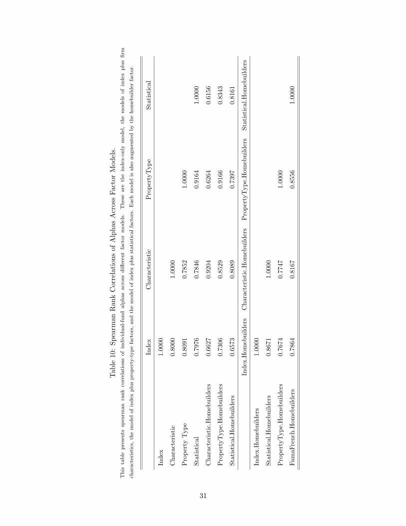
Tab

le10

:Sp

earm

anR

ank

Cor

rela

tion

sof

Alp

has

Acr

oss

Fact

orM

odel

s.T

his

table

pre

sents

spea

rman

rank

corr

elations

of

indiv

idual-fu

nd

alp

has

acr

oss

diff

eren

tfa

ctor

model

s.T

hes

eare

the

index

-only

model

,th

em

odel

sof

index

plu

sfirm

chara

cter

istics

,th

em

odel

ofin

dex

plu

spro

per

ty-t

ype

fact

ors

,and

the

model

ofin

dex

plu

sst

atist

icalfa

ctors

.E

ach

model

isals

oaugm

ente

dby

the

hom

ebuilder

fact

or.

Inde

xC

hara

cter

isti

cP

rope

rtyT

ype

Stat

isti

cal

Inde

x1.

0000

Cha

ract

eris

tic

0.80

001.

0000

Pro

pert

yT

ype

0.80

910.

7852

1.00

00

Stat

isti

cal

0.79

760.

7846

0.91

641.

0000

Cha

ract

eris

tic.

Hom

ebui

lder

s0.

6627

0.92

040.

6264

0.61

56

Pro

pert

yTyp

e.H

omeb

uild

ers

0.73

060.

8529

0.91

660.

8343

Stat

isti

cal.H

omeb

uild

ers

0.65

730.

8089

0.73

970.

8161

Inde

x.H

omeb

uild

ers

Cha

ract

eris

tic.

Hom

ebui

lder

sP

rope

rtyT

ype.

Hom

ebui

lder

sSt

atis

tica

l.Hom

ebui

lder

s

Inde

x.H

omeb

uild

ers

1.00

00

Stat

isti

cal.H

omeb

uild

ers

0.86

711.

0000

Pro

pert

yTyp

e.H

omeb

uild

ers

0.76

740.

7747

1.00

00

Fam

aFre

nch.

Hom

ebui

lder

s0.

7864

0.81

670.

8556

1.00

00

31

Table 11: Fund Performance as a Function of Fund Characteristics.This table presents results from Fama-Macbeth (1973) regressions of annual fund returns (before fees) on a constant, the natural

logarithm of the fund’s total NAV lagged by one year, expense ratio, turnover, number of holdings, and a load indicator which

is equal to one if the fund has a nonzero front or rear load and zero otherwise.

Coefficient t-statistic

Before Expenses

Intercept 0.1619 2.2765◦

Ln(Sizet−1) 0.0005 0.3960

Expenses -0.5314 −0.6731

Turnover 0.0182 1.7709

Holdings −0.0001 −0.7128

Load 0.0021 0.3049

Average R2 0.0877

◦: p < 10%; ∗: p < 5%; ∗∗: p < 1%; ∗∗∗: p < 0.1%. 8 time-series observations.

32

Figure 1: Box and whisker diagrams of the distrbutions of alphas generated by the single indexmodel, and four different models including Homebuilders. The heavy line in the middle of each boxindicates the median, the lower and upper edges indicate the first- and third quartiles respectively,while the whiskers extend 1.5 times the interquartile range outward from the edge of the box. Anyoutliers that lie beyond this distance are indicated individually by a circle. Index represents thealphas from a model of the Dow Jones Wilshire REIT Index only. Char, Prop, and Stat denotemodels using the single Index, plus the chracteristic factors, property factors, and statistical factors,respectively. The suffix “.HB” indicates models that include the Homebuilders index.

Index Index.HB Char.HB Prop.HB Stat.HB

−0.010

−0.005

0.000

0.005

Distributions of Alphas

33