Policy Research Working Paper 7338

Euro Currency Risk and the Geography of Debt Flows to Peripheral European

Monetary Union MembersEylem Ersal-Kiziler

Ha Nguyen

Development Research GroupMacroeconomics and Growth TeamJune 2016

WPS7738P

ublic

Dis

clos

ure

Aut

horiz

edP

ublic

Dis

clos

ure

Aut

horiz

edP

ublic

Dis

clos

ure

Aut

horiz

edP

ublic

Dis

clos

ure

Aut

horiz

edP

ublic

Dis

clos

ure

Aut

horiz

edP

ublic

Dis

clos

ure

Aut

horiz

edP

ublic

Dis

clos

ure

Aut

horiz

edP

ublic

Dis

clos

ure

Aut

horiz

edP

ublic

Dis

clos

ure

Aut

horiz

edP

ublic

Dis

clos

ure

Aut

horiz

edP

ublic

Dis

clos

ure

Aut

horiz

edP

ublic

Dis

clos

ure

Aut

horiz

edP

ublic

Dis

clos

ure

Aut

horiz

edP

ublic

Dis

clos

ure

Aut

horiz

edP

ublic

Dis

clos

ure

Aut

horiz

edP

ublic

Dis

clos

ure

Aut

horiz

edP

ublic

Dis

clos

ure

Aut

horiz

edP

ublic

Dis

clos

ure

Aut

horiz

edP

ublic

Dis

clos

ure

Aut

horiz

edP

ublic

Dis

clos

ure

Aut

horiz

ed

Produced by the Research Support Team

Abstract

The Policy Research Working Paper Series disseminates the findings of work in progress to encourage the exchange of ideas about development issues. An objective of the series is to get the findings out quickly, even if the presentations are less than fully polished. The papers carry the names of the authors and should be cited accordingly. The findings, interpretations, and conclusions expressed in this paper are entirely those of the authors. They do not necessarily represent the views of the International Bank for Reconstruction and Development/World Bank and its affiliated organizations, or those of the Executive Directors of the World Bank or the governments they represent.

Policy Research Working Paper 7338

This paper is a product of the Macroeconomics and Growth Team, Development Research Group. It is part of a larger effort by the World Bank to provide open access to its research and make a contribution to development policy discussions around the world. Policy Research Working Papers are also posted on the Web at http://econ.worldbank.org. The authors may be contacted at hanguyen@worldbank.org.

The pattern of debt flows to peripheral European Monetary Union members seems puzzling: they are mostly indirect and channeled through the large countries of the Euro-pean Monetary Union. This paper examines to what extent the introduction of the euro and the elimination of the intra-area currency risk can explain this puzzle. A three-country dynamic stochastic general equilibrium framework with endogenous portfolio choice and two currencies is

developed. In the equilibrium, the core members of the European Monetary Union emerge as the main group of lenders to the peripheral European Monetary Union mem-bers. Outside lenders are pushed from the periphery debt markets because of currency risk. The model generates a pattern of debt flows consistent with the data despite the absence of any exogenous frictions or market segmentations.

Euro Currency Risk and the Geography of Debt Flows to PeripheralEuropean Monetary Union Members

Eylem Ersal-Kizilera,∗, Ha Nguyenb

aUniversity of Wisconsin - Whitewater, Department of Economics, 809 W. Starin Road, Whitewater, WI 53190, USAbWorld Bank, Development Research Group, 1818 H Street NW, Washington D.C. 20433, USA

1. Introduction

Hale and Obstfeld (2016) and Hobza and Zeugner (2014) document an interesting and puzzling

empirical fact: since the foundation of the EMU, the financing of peripheral EMU members’ trade

deficits versus the rest of the world was mostly indirect and intermediated by the large countries of

the core EMU.1 Peripheral EMU’s debts were held mainly by Germany and France.2 In turn, core

EMU’s debts were largely held by outside investors.

It is puzzling why investors outside the euro area are more reluctant to hold periphery bonds, and

the core EMU countries hold an overwhelming portion of periphery bonds. Why do outsiders not

lend to peripheral EMU directly? Using a stylized model, Hale and Obstfeld (2016) argue that this is

because the transaction costs of lending to the peripheral EMU are lower for the core EMU than for the

rest of the world. Coeurdacier and Martin (2009) find that preferential financial liberalization lowers

transaction costs inside the Eurozone (relative to outside the Eurozone) by about 17% for bonds and

10% for stocks. Kalemli-Ozcan et al. (2010) consider three potential candidates to explain financial

integration within the EMU: elimination of currency risk, legal harmonization and trade. They find

that the elimination of currency risk is the primary explanation for the increasing integration.

In this paper, we theoretically investigate the role of currency risk, and its impact on the geographic

pattern of debt flows to the peripheral EMU. We argue that the core EMU has a clear advantage

compared to the outside lenders when lending to the peripheral EMU. Core countries share the same

currency with the periphery and are not concerned about the currency risk. Due to this advantage,

core EMU lenders can push outside lenders out of the periphery bond market.

However, we do not underestimate the importance of other factors that might have caused this

market segmentation. Hale and Obstfeld (2016) argue that four main factors contributed to the

comparative advantage of the core EMU in lending to the periphery: the decline in (perceived) risks

of investing in the peripheral EMU, the decline in transaction costs and the elimination of the currency

risk, the European Central Bank‘s policy of applying an identical collateral haircut to all euro area

sovereigns, regardless of their varied credit ratings, and uniform financial regulations within the euro

∗Corresponding authorEmail addresses: kizilere@uww.edu (Eylem Ersal-Kiziler), hanguyen@worldbank.org (Ha Nguyen)

1Peripheral EMU refers to Portugal, Italy, Ireland, Greece, and Spain. Core EMU refers to mainly Germany andFrance.

2Previous empirical studies such as Lane and Milesi-Ferretti (2005), Lane (2006), Spiegel (2009), De Santis andGrard (2009) and Haselmann and Herwartz (2010) ... also highlight the euro bias as an explanation to the euro areacountries’ increasing investments in other euro area countries after the formation of the EMU.

area. Another factor is zero risk weights. The current regulatory framework grants EMU banks a

beneficial treatment of credit risk on their sovereign debt exposures by assigning 0% risk weights,

essentially exempting sovereign exposure (Acharya and Steffen (2015)). In addition, the lack of large

exposure rule for public debt allows core EMU banks to take on a very large position on peripheral

debt. Banks outside the Eurozone, however, do not have that advantage. Information asymmetry

might have also contributed to the observed geographic pattern of flows. Information asymmetry

refers to the fact that the core EMU lenders know and understand the peripheral EMU borrowers

better than outsiders. This is a possibility and can very well be true for private individuals and banks,

but to a lesser extent for sovereign bonds.

In our paper, we focus on the role of the currency risk in shaping the direction of the debt flows.

We show that in a calibrated three-country DSGE model, with the presence of euro currency risk

and no other frictions, the core EMU lenders can hold a large part of the periphery’s debt, pushing

outsiders out of the peripheral EMU’s debt markets. To the best of our knowledge, our paper is

the first to analyze the geographic pattern of debt flows using a DSGE portfolio choice approach.

Engel and Matsumoto (2009), Coeurdacier and Gourinchas (2011) and Bengui and Nguyen (2011)

also study optimal portfolio choice in the presence of exchange rate risk. However, the issues they

examine are different. Engel and Matsumoto (2009) and Coeurdacier and Gourinchas (2011) focus

on explaining the equity home bias puzzle. In symmetric two-country setups, they show that not

much equity diversification is required when agents can hedge their foreign exchange risk sufficiently.

Bengui and Nguyen (2011) examine international debt dollarization in a small open economy setup.

Our paper, on the other hand, investigates the pattern of debt flows as an optimal portfolio choice in

a three-country setup.

Intuitively, there are two competing channels that influence the portfolio decisions of the core

EMU and outside investors. The first channel is called the “currency channel”. It refers to the fact

that the core EMU shares the same currency with the periphery. This currency advantage allows

them to absorb the bad shocks to the periphery bonds’ returns better than outside investors do. The

mechanism works as follows. Consider the core EMU holders and the U.S. holders of the periphery

bonds. If the euro depreciates against the U.S. dollar (for instance, because of an increase in the euro

money supply), the dollar value of the periphery bond’s return declines. This hurts both core EMU

and U.S. bond holders. Furthermore, when the non-tradable good prices are sticky, the dollar value

of the consumption expenditure of the core EMU bond holder is going to be lower compared to the

U.S. bond holder.3 This helps the core EMU bond holders. Since the U.S. lenders only consume in

dollars, they do not have this advantage. Even when the law of one price holds for tradable goods,

the existence of non-tradable goods and nominal rigidity enable the “currency channel” to work in

favor of the core EMU lenders.4 Simply put, being in the same monetary union with the periphery

gives the core EMU an advantage over outside lenders in terms of lending to the peripheral EMU.

The second channel is called “the business cycle channel” and it discourages the core EMU lenders

from lending to the peripheral EMU. It works as follows: core EMU countries’ business cycles are

3For example, a 10 euro haircut previously cost 14 dollars. When the euro depreciates and dollar prices are sticky,a 10 euro haircut now costs only 12 dollars.

4Nominal shocks, such as currency risk, only work in the presence of nominal rigidity. If prices are completelyflexible, nominal shocks would have no real impact.

2

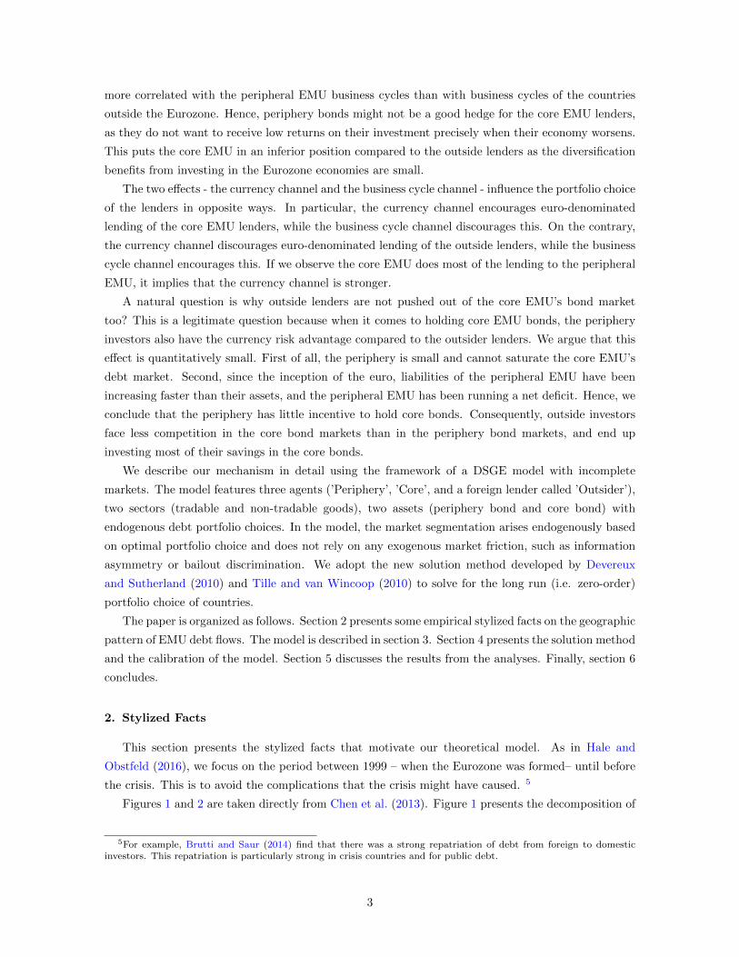
more correlated with the peripheral EMU business cycles than with business cycles of the countries

outside the Eurozone. Hence, periphery bonds might not be a good hedge for the core EMU lenders,

as they do not want to receive low returns on their investment precisely when their economy worsens.

This puts the core EMU in an inferior position compared to the outside lenders as the diversification

benefits from investing in the Eurozone economies are small.

The two effects - the currency channel and the business cycle channel - influence the portfolio choice

of the lenders in opposite ways. In particular, the currency channel encourages euro-denominated

lending of the core EMU lenders, while the business cycle channel discourages this. On the contrary,

the currency channel discourages euro-denominated lending of the outside lenders, while the business

cycle channel encourages this. If we observe the core EMU does most of the lending to the peripheral

EMU, it implies that the currency channel is stronger.

A natural question is why outside lenders are not pushed out of the core EMU’s bond market

too? This is a legitimate question because when it comes to holding core EMU bonds, the periphery

investors also have the currency risk advantage compared to the outsider lenders. We argue that this

effect is quantitatively small. First of all, the periphery is small and cannot saturate the core EMU’s

debt market. Second, since the inception of the euro, liabilities of the peripheral EMU have been

increasing faster than their assets, and the peripheral EMU has been running a net deficit. Hence, we

conclude that the periphery has little incentive to hold core bonds. Consequently, outside investors

face less competition in the core bond markets than in the periphery bond markets, and end up

investing most of their savings in the core bonds.

We describe our mechanism in detail using the framework of a DSGE model with incomplete

markets. The model features three agents (’Periphery’, ’Core’, and a foreign lender called ’Outsider’),

two sectors (tradable and non-tradable goods), two assets (periphery bond and core bond) with

endogenous debt portfolio choices. In the model, the market segmentation arises endogenously based

on optimal portfolio choice and does not rely on any exogenous market friction, such as information

asymmetry or bailout discrimination. We adopt the new solution method developed by Devereux

and Sutherland (2010) and Tille and van Wincoop (2010) to solve for the long run (i.e. zero-order)

portfolio choice of countries.

The paper is organized as follows. Section 2 presents some empirical stylized facts on the geographic

pattern of EMU debt flows. The model is described in section 3. Section 4 presents the solution method

and the calibration of the model. Section 5 discusses the results from the analyses. Finally, section 6

concludes.

2. Stylized Facts

This section presents the stylized facts that motivate our theoretical model. As in Hale and

Obstfeld (2016), we focus on the period between 1999 – when the Eurozone was formed– until before

the crisis. This is to avoid the complications that the crisis might have caused. 5

Figures 1 and 2 are taken directly from Chen et al. (2013). Figure 1 presents the decomposition of

5For example, Brutti and Saur (2014) find that there was a strong repatriation of debt from foreign to domesticinvestors. This repatriation is particularly strong in crisis countries and for public debt.

3

Fig. 1. Net foreign assets of peripheral EMU. Source: Chen et al. (2013).

Fig. 2. Net foreign assets of core EMU. Source: Chen et al. (2013).

the peripheral EMU’s net foreign asset position versus other euro area countries and versus the rest

of the world. The figure shows that net liabilities versus other euro area countries accounted for the

lion share of the peripheral EMU’s net liabilities since the beginning of 2000s. In 2001, the core held

about 60 percent of the periphery’s net liabilities. This share was about 75 percent by 2008. Figure 2

shows the decomposition of the core EMU’s net foreign asset position versus other euro area countries

and versus the rest of the world. Core EMU’s net foreign assets were primarily versus the rest of the

euro area (i.e. peripheral EMU), while their liabilities were mostly versus the rest of the world.

Hale and Obstfeld (2016) illustrate the changes in debt flows to core and periphery countries after

the inception of the euro very clearly. Figure 3 is borrowed from their paper. They organize the

countries to 4 groups: financial centers (FIN), core EMU (CORE), peripheral EMU (GIIPS) and the

rest of the world (ROW)6. Data are from the Bank of International Settlement’s consolidated banking

6FIN consists of Canada, Denmark, Japan, Sweden, Switzerland, UK, and US; CORE consists of Austria, Belgium,Finland, France, Germany, Netherlands, Luxembourg; GIIPS consists of Greece, Italy, Ireland, Portugal and Spain.

4

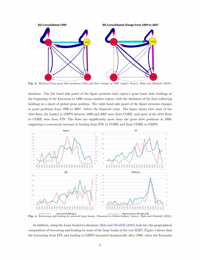
Fig. 3. Bilateral bank gross debt positions (left) and their change by 2007 (right). Source: Hale and Obstfeld (2016).

database. The left hand side panel of the figure presents each region’s gross bank debt holdings at

the beginning of the Eurozone in 1999 versus another region, with the thickness of the lines reflecting

holdings as a share of global gross position. The right hand side panel of the figure presents changes

in gross positions from 1999 to 2007– before the financial crisis. The figure shows that most of the

debt flows (by banks) to GIIPS between 1999 and 2007 were from CORE, and most of the debt flows

to CORE were from FIN. The flows are significantly more than the gross debt positions in 1999,

suggesting a concurrent increase in lending from FIN to CORE and from CORE to GIIPS.

Fig. 4. Borrowing and lending by selected large banks. Measured in billion dollars. Source: Hale and Obstfeld (2016).

In addition, using the Loan Analytics database, Hale and Obstfeld (2016) look into the geographical

composition of borrowing and lending by some of the large banks in the core EMU. Figure 4 shows that

the borrowing from FIN and lending to GIIPS increased dramatically after 1999, when the Eurozone

5

was formed, but collapsed during the 2008-2009 crisis. They find that there is a link between core

EMU banks’ borrowing from FIN and their lending to GIIPS during the pre-crisis period. This is as

if the banks intermediated loans to the peripheral EMU. They do not find such a link for banks in

different regions.7

It is interesting that both the lending from FIN to the core EMU banks and lending from the

core EMU banks to GIIPS collapsed during the crisis. This phenomenon could be explained by an

increase in risk aversion of all lenders during this time (Guiso et al. (2013)), and a perceived higher

default risk, particularly of GIIPS countries. Higher risk aversion and higher default risk would cause

capital to retrench. Currency risk during the crisis might have become secondary, and might have

been overshadowed by these factors.

3. Model

We build a three-country, two-asset model to formalize our theory. The three countries are Pe-

riphery (denoted P), Core (denoted C) and Outsider (denoted O). P and C share the same currency

(euros) while O uses dollars. The two assets are Periphery bonds and Core bonds, issued in euros. P

only issues its Periphery bonds, and is assumed not to hold Core bonds. C can hold Periphery bonds,

and issue its Core bonds. O has a choice of holding Periphery bonds and Core bonds. We also assume

that the nominal bonds’ returns are state contingent: they depend on the output realization.

We assume that country P does not hold Core bonds. This assumption not only makes the model

more tractable, but also is aligned with the empirical evidence. It allows us to imitate the borrowing

nature of the periphery countries since the inception of the euro. Therefore, we are able to focus on

the competition between the Core and the Outsider lenders over the Periphery debt and hence analyze

the currency risk and business cycle channels with more clarity. Similarly, we do not allow the outside

country to issue debt, as it does not contribute to the answering of the question at hand.

In each of the three economies, households provide labor and consume tradable and non-tradable

goods. Firms produce non-tradable goods, and return profit to households. Households transfer wealth

across time by holding or issuing bonds. While the country-specific non-tradable good is produced

using labor, for simplicity, we assume that there is a single tradable good and each country receives an

endowment of this good according to a country-specific stochastic process. The non-tradable goods’

prices are sticky, while the tradable good’s price is flexible. As a standard convention in the New

Keynesian models, nominal rigidities in the non-tradable sector are modeled by dividing the sector

into perfectly competitive retailers and monopolistically competitive intermediate good producers. In

addition, in the model we assign Periphery and Core a higher discount rate to generate their borrowing

from the Outsider in the equilibrium.

3.1. Notation

To be clear from the beginning, let us go through some of the key notation used in the paper.

Superscripts P, C, and O denote country P (Periphery), C (Core), and O (Outsider).

7Refer to Hale and Obstfeld (2016) for more detailed analysis with different data sources.

6

(cPTt, cPNt, c

Pt ), (cCTt, c

CNt, c

Ct ) and (cOTt, c

ONt, c

Ot ) are the tradable, non-tradable, and aggregate con-

sumption of Periphery, Core and Outsider countries, respectively.

PPNt, PCNt, P

ONt are the nominal non-tradable good prices of Periphery, Core and Outsider countries,

respectively.

PETt, POTt are the nominal tradable good prices of the Eurozone and Outsider countries, respectively.

8

PPt , PCt , P

Ot are the nominal aggregate prices of Periphery, Core and Outsider countries, respec-

tively.

bjit is country j’s holding of country i’s bond in units of the tradable good. We refer to them as

the “real” bond holdings.

3.2. Periphery Country

The expected life-time utility of a representative Periphery household is given by:

E0

∞∑t=0

ψPt

1

1 − σ

(cPt − Φ

lP1+νt

1 + ν

)1−σ

+ χ ln

(MPt

PPt

)Households derive utility from aggregate consumption (cPt ), real money holdings (

MPt

PPt) and experience

disutility from working. The utility takes the form of GHH utility function to remove wealth effects

and hence generate a decline in employment in bad times.9 Aggregate consumption consists of tradable

and non-tradable consumption:

cPt =(cPTt)

γ(cPNt)1−γ

γγ(1 − γ)1−γ .

Hence the aggregate price takes the form:

PPt = (PETt)γ(PPNt)

1−γ ,

ψPt ≡ (φPβ)tΠtk=0c

P−µTk is country P’s discount factor. It has two components. (φPβ)t is the

standard discount factor component. φP is the coefficient reflecting country P’s patience.10 The

second component Πtk=0c

P−µTk is the (uninternalized) endogenous discount factor that depends on the

aggregate (economy-wide) level of households’ tradable consumption. As in Schmitt-Grohe and Uribe

(2003), this is a simple technical device to induce uniqueness of the deterministic steady state and

stationary responses to temporary shocks. Specifically, the endogenous discount factor decreases with

the aggregate tradable consumption, which the representative household takes as given. In addition,

µ = 0.001 is set very small so that in the short run, the deviations of the endogenous discount factor

from the standard discount factor β are negligible.

8Note that Periphery and Core share the same nominal tradable price, since they have the same currency.9See Greenwood et al. (1988) for further details.

10Similarly, φC and φO are the patience coefficients for countries C and O. To ensure Outsider lends to Peripheryand Core, we assume that O is more patient (i.e. φO > φC and φO > φP ).

7

Households face a sequence of budget constraints:

PETtcPTt + PPNtc

PNt + PETtb

PPt +MP

t =

yPTtRPt−1P

ETt−1b

PPt−1 +MP

t−1 +WPt l

Pt + PETty

PTt +DP

t−1, (1)

where bPPt is the “real” Periphery bond holdings of country P’s households (a negative bPP implies

issuing). MPt is the money holding. yPTtR

Pt is the ex-post nominal return of the Periphery bond,

which depends on P’s output and the nominal interest rate RPt−1 , which was determined in the last

period when the bond was issued. WPt is the nominal wage, yPTt is the tradable endowment, and DP

t−1

is the profit from non-tradable production returned by firms at the end of the last period (since firms

are owned by households).

The first-order conditions of the household’s problem are:

PPNtPETt

=1 − γ

γ

cTtcNt

(2)

Φlνt =γcγ−1Tt c1−γNt

γγ(1 − γ)1−γWPt

PETt(3)

U ′cTt(.) = φPβc−µt Etr

Pt+1U

′cTt+1

(.) (4)

U ′cTt(.) = χPETtMPt

+ φPβc−µt Et

PETtPETt+1

U ′cTt+1(.) (5)

where, for brevity, the superscript P is dropped for consumption and labor variables. rPt+1 =

RPtPETtPETt+1

yPTt+1 and rCt+1 = RCtPETtPETt+1

yCTt+1 denote the ex-post real returns of country P and coun-

try C’s bonds, respectively. In the first-order conditions, marginal utility with respect to tradable

consumption is denoted as U ′cTt(.) ≡(ct − Φ

l1+νt

1+ν

)−σγcγ−1Tt c1−γNt

γγ(1−γ)1−γ . Equation (2) is a static optimality

condition describing the composition of the household’s consumption basket between tradable and

non-tradable goods. Equation (3) is a static optimality condition describing the labor choice of the

consumer. Equations (4) and (5) are Euler equations for Periphery bonds, and money holdings,

respectively.

We now move to firms. Intermediate producer j produces a differentiated intermediate non-

tradable good yPNjt using constant technology AN and labor lPjt according to a linear production

function

yPNjt = AN lPjt

To model nominal rigidities in the non-tradable market, we separate the non-tradable sector into

intermediate good producers and retailers. Producers sell their output to competitive retailers who

combine these intermediate goods to produce a final good using a constant elasticity of substitution

(CES) production function

Y PNt =

[∫ 1

0

yPωF−1

ωF

Njt

] ωFωF−1

,

where ωF is the elasticity of substitution between any two differentiated intermediate non-tradable

goods, and ωF1−ωF is the firm’s markup.

8

The nominal profit of producer j is:

DPjt = PPNjtAN l

Pjt −WP

t lPjt (6)

where DPjt is the profit that the producer distributes to households at the end of the period, for

consumption in the next period.

In each period, only a fraction 1 − κ of the firms can adjust price. This means that for each firm,

at the beginning of each period, there is a constant probability of 1 − κ that they can change their

price if they want to. If the firm had fully flexible price (κ = 0), it would set the (hypothetical) price

as a mark-up over marginal cost.

P ∗PNt =ωF

ωF − 1MCPt =

ωFωF − 1

WPt

AN

As is standard in New-Keynesian (NK) models, the aggregate non-tradable price for country P is

governed by the following equation:

logPPNt − logPPNt−1 = (cPt )−µφPβEt(logPPNt+1 − logPPNt)

+ λF

(log

(WPt

PPNtAN

)− log

(WP

PPN AN

))(7)

where λF =(1−κ)(1−(cPt )−µφP βκ)

κ , and X denotes the steady state value of a variable.

3.3. Core Country and Outsider Country

The setup for country C and country O is quite similar to the setup for country P. The differences

are (1) C and O have different discount factors, and (2) unlike P, who only can issue Periphery bonds,

C can issue Core bonds and hold Periphery bonds, and O can hold both Periphery and Core bonds

. For country C, the discount factor is ψCt ≡ (φCβ)tΠtk=0c

C−µTk . For country O, the discount factor

is ψOt ≡ (φOβ)tΠtk=0c

O−µTk . Note that we assume φO > φP and φO > φC so that Outsider lends to

Periphery and Core in the equilibrium.

The expected life-time utility of a representative Core household is given by:

E0

∞∑t=0

ψCt

1

1 − σ

(cCt − Φ

lC1+νt

1 + ν

)1−σ

+ χ ln

(MCt

PCt

)Households face a sequence of budget constraints

PETtcCTt + PCNtc

CNt + PETtb

CPt + PETtb

CCt +MC

t =

yCTtRCt−1P

ETt−1b

CCt−1 + yPTtR

Pt−1P

ETt−1b

CPt−1 +MC

t−1 +WCt l

Ct + PETty

CTt +DC

t−1 (8)

where bCPt is the “real” Periphery bond holdings of country C’s households, bCCt is the “real” Core

bond holdings of country C’s households (a negative bCC implies issuing).

9

The first-order conditions of the Core household’s problem are:

PCNtPETt

=1 − γ

γ

cTtcNt

(9)

Φlνt =γcγ−1Tt c1−γNt

γγ(1 − γ)1−γWCt

PETt(10)

U ′cTt(.) = φCβc−µt Etr

Pt+1U

′cTt+1

(.) (11)

U ′cTt(.) = φCβc−µt Etr

Ct+1U

′cTt+1

(.) (12)

U ′cTt(.) = χPETtMCt

+ φCβc−µt Et

PETtPETt+1

U ′cTt+1(.) (13)

where, for brevity, the superscript C is dropped for consumption and labor variables. Equation (9) is a

static optimality condition describing the composition of the household’s consumption basket between

tradable and non-tradable goods. Equation (10) is a static optimality condition describing the labor

choice of the consumer. Equations (11), (12) and (13) are Euler equations for Periphery bonds, Core

bonds and money holdings, respectively.

The expected life-time utility of a representative Outsider household is given by:

E0

∞∑t=0

ψOt

1

1 − σ

(cOt − Φ

lO1+νt

1 + ν

)1−σ

+ χ ln

(MOt

POt

)Households face a sequence of budget constraints

POTtcOTt + PONtc

ONt + POTtb

OPt + POTtb

OCt +MO

t =

yCTtRCt−1P

OTtb

OCt−1

PETt−1

PETt+ yPTtR

Pt−1P

OTtb

OPt−1

PETt−1

PETt+MO

t−1 +WOt l

Ot + POTty

OTt +DO

t−1 (14)

where bOPt is the real Periphery bond holdings of country O’s households, bOCt is the real Core bond

holdings of country O’s households.

The first-order conditions of the Outsider household’s problem are:

PONtPOTt

=1 − γ

γ

cTtcNt

(15)

Φlνt =γcγ−1Tt c1−γNt

γγ(1 − γ)1−γWOt

POTt(16)

U ′cTt(.) = φOβc−µt Etr

Pt+1U

′cTt+1

(.) (17)

U ′cTt(.) = φOβc−µt Etr

Ct+1U

′cTt+1

(.) (18)

U ′cTt(.) = χPOTtMOt

+ φOβc−µt Et

POTtPOTt+1

U ′cTt+1(.) (19)

where for brevity, the superscript O is dropped for consumption and labor variables.

10

3.4. Exogenous Shocks

There are real and nominal shocks in the model. Real shocks are shocks to the tradable good

endowments of the three countries:

log(yPTt) = ρP log(yPTt−1) + (1 − ρP )log(yP ) + εPt (20)

log(yCTt) = ρC log(yCTt−1) + (1 − ρC)log(yC) + εCt (21)

log(yOTt) = ρOlog(yOTt−1) + (1 − ρO)log(yO) + εOt (22)

Nominal shocks are the shocks to the supply of euros and dollars:

log(MEt ) = ρMElog(ME

t−1) + εMEt (23)

log(MOTt) = ρMOlog(MO

t−1) + εMOt (24)

3.5. Market Clearings

Tradable good market clearing implies:

cOTt + cCTt + cPTt = yOTt + yCTt + yPTt (25)

Both Periphery and Core bonds are in zero net supply. Market clearing for bond markets imply:

bPPt + bCPt + bOPt = 0 (26)

and

bCCt + bOCt = 0 (27)

The first bond market clearing equation implies that Periphery issued bonds are entirely held by C

and O. The second equation implies that Core issued bonds are entirely held by O.

Since country P and country C share the euro supply, euro money market clearing implies that

euro holdings by country P and C add up to the total euro supply.

MEt = MP

t +MCt (28)

4. Model Solution and Calibration

It is well-known that up to the first-order approximation, the values of the portfolio choices are

indeterminate, because at this level of approximation, the two assets are perfect substitutes. Previous

literature usually relies on complete asset market structures that make portfolio choice irrelevant.

Since the focus of our paper is on the bond choices, we will adopt the solution method developed

by Devereux and Sutherland (2010) and Tille and van Wincoop (2010) to solve for the steady state

portfolio bond holdings of the Core and Outsider lenders.

4.1. Solving for the Portfolio Holdings

We use the approach of Devereux and Sutherland (2010) and Tille and van Wincoop (2010) to

solve the steady state portfolio choice problem. The portfolio choices of country C and country O

11

should satisfy the following:

Et(rPt+1 − rCt+1

)(U ′cOTt+1

(.) − U ′cCTt+1(.)) = 0 (29)

Equation (29) means that C and O will choose an optimal bond portfolio so that the differential

in their marginal utilities on average is not correlated to the return differential of their bond holdings.

In other words, their consumption is on average insured against the monetary shocks and real shocks

to P and C’s tradable endowments.

Taking a second-order logarithmic approximation of the country C and country O portfolio first-

order conditions and combining them yields:

Et[(rCt+1 − rPt+1)(coOctc

Ot+1 + coOcnc

Ot+1 + coOl l

Ot+1 − coCctc

Ct+1 − coCcnc

Ct+1 − coCl l

Ct+1)] = 0, (30)

where x denotes log deviations from the steady state value of the variable. coij are the coefficients on

variable j of country i and they are as follows: coict = γ − 1 − σγ ci

ci−Φ li1+ν

1+ν

, coicn = 1 − γ − σ(1 −

γ) ci

ci−Φ li1+ν

1+ν

, coil = σΦ li1+ν

ci−Φ li1+ν

1+ν

.

The details of the solution method are presented in Appendix A.

4.2. Baseline Calibration and the Steady State

The value of the discount factor is set for quarterly data: β = 0.98. The share of tradable

consumption is a third of total consumption: γ = 13 . Following Chugh (2006), we set χ equal 0.05,

the elasticities of substitution ωF = 10. We set the endogenous discount factor coefficient very small

µ = 0.001, so that it does not have a significant impact on the model’s dynamics. We also set the

persistence of money supply to 0.9, and the persistence of endowment to 0.8. We set κ equal to 0.75,

implying that the average period between price adjustments is four quarters, as in Bernanke et al.

(1999). The correlations of P, C and O’s endowments are consistent with the data.11

The steady state of the three-economy system is summarized in Table 2 and they seem quite

reasonable. Overall, the share of the non-tradable good value is about two-thirds of total consumption

in all the economies. Country P’s net foreign asset position is negative (which means P is borrowing)

and about -100 % of its total output, whereas the size of countries O and C’s NFA position ranges

from about 40% to 60% of their total output. The next section will discuss the steady state values of

the bond portfolio holdings.

5. Results

In this section we introduce the results of the model. First, we present the steady state portfolio

holdings. Using three exercises, we demonstrate the importance of the business cycle and the currency

risk channels by studying the changes in the steady state portfolio holdings in response to the changes

11Peripheral EMU consists of Italy, Spain, Portugal, Greece. Core EMU consists of France, Germany, Belgium.Outsider economies consist of United States, United Kingdom, Switzerland and Japan. Data is obtained from theOECD. For each group, we divide the total quarterly real GDP by the total population to obtain the group quarterlyreal GDP per capita. The moments are calculated from the series of the groups’ quarterly real GDP growth.

12

Table 1Baseline calibration

Description Valueγ Share of tradable consumption 0.33χ Utility from money holdings 0.05β Discount factor 0.98µ Endogenous discount factor coefficient 0.001AN TFP in intermediate non-tradable good production 1ωF Elasticity of subs. betw. intermediate non-tradable goods 10ρm Persistence of money supply 0.9σm Standard deviation of money supply 0.001κ Non-tradable good price stickiness 0.75ρP Persistence of P’s tradable endowment 0.8ρC Persistence of C’s tradable endowment 0.8ρO Persistence of O’s tradable endowment 0.8σP Standard deviation of P’s tradable endowment 0.01σC Standard deviation of C’s tradable endowment 0.01σO Standard deviation of O’s tradable endowment 0.01ρ(P,C) Correlation between P and C’s tradable endowment 0.9ρ(P,O) Correlation between P and O’s endowment 0.2ρ(C,O) Correlation between C and O’s endowment 0.3ν Utility from leisure 0.6Φ Disutility from labor 3φP Patience parameter for Periphery 0.9999φC Patience parameter for Core 0.99999φO Patience parameter for Outsider 1

in the influence of each channel. Further, we discuss the mechanism in which these channels operate

using the impulse responses to nominal and real shocks.

5.1. Steady State Portfolio Holdings

Under the baseline calibration displayed in Table 1, and using a value of 0.75 for the price stickiness

parameter κ, we find that Core holds 65% of the Periphery debt and the remainder 35% of the

Periphery liabilities is held by the Outsider investor. This is aligned with the data (see Figure 1).

To evaluate the relative importance of the business cycle and the currency risk channels on the

portfolio holdings, we perform three exercises. In these exercises, we vary the value of the price

stickiness parameter κ and the correlation between the three countries’ endowments.

We change κ in order to capture varying degrees of currency risk exposure. A larger value for

κ means higher degree of price stickiness in the non-tradable goods, which we interpret as higher

exposure to currency risk. We predict that, everything else constant, when non-tradable good prices

are sticky, a depreciation of the euro lowers the dollar value of Core household’s non-tradable good

consumption expenditure, which gives them an advantage over the Outsider household. In contrast,

flexible non-tradable good prices could leave the dollar value of non-tradable good consumption ex-

penditure unaffected, invalidating the currency risk.

The importance of the business cycle channel is adjusted by changing the endowment correlation

between countries P and C, and between countries P and O. When a country’s endowment is more

correlated with country P’s endowment, their incentive to lend to country P is weakened.

13

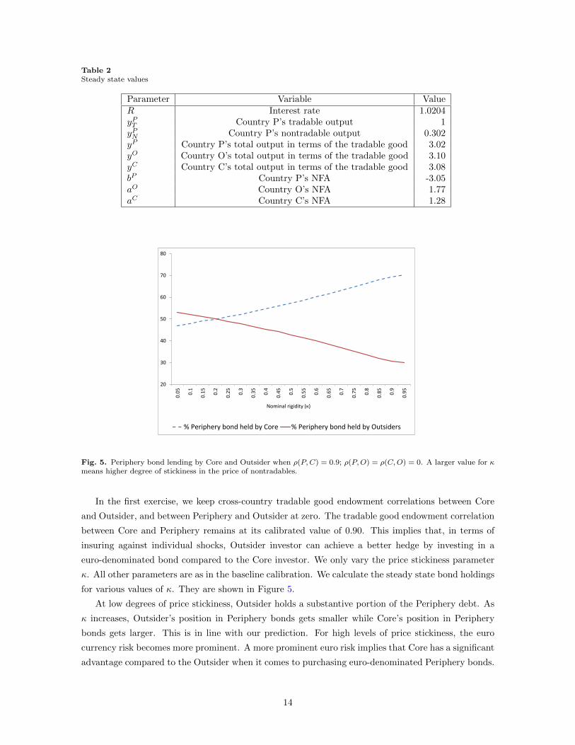
Table 2Steady state values

Parameter Variable ValueR Interest rate 1.0204yPT Country P’s tradable output 1yPN Country P’s nontradable output 0.302yP Country P’s total output in terms of the tradable good 3.02yO Country O’s total output in terms of the tradable good 3.10yC Country C’s total output in terms of the tradable good 3.08bP Country P’s NFA -3.05aO Country O’s NFA 1.77aC Country C’s NFA 1.28

20

30

40

50

60

70

80

0.0

5

0.1

0.1

5

0.2

0.2

5

0.3

0.3

5

0.4

0.4

5

0.5

0.5

5

0.6

0.6

5

0.7

0.7

5

0.8

0.8

5

0.9

0.9

5Nominal rigidity (к)

% Periphery bond held by Core % Periphery bond held by Outsiders

Fig. 5. Periphery bond lending by Core and Outsider when ρ(P,C) = 0.9; ρ(P,O) = ρ(C,O) = 0. A larger value for κmeans higher degree of stickiness in the price of nontradables.

In the first exercise, we keep cross-country tradable good endowment correlations between Core

and Outsider, and between Periphery and Outsider at zero. The tradable good endowment correlation

between Core and Periphery remains at its calibrated value of 0.90. This implies that, in terms of

insuring against individual shocks, Outsider investor can achieve a better hedge by investing in a

euro-denominated bond compared to the Core investor. We only vary the price stickiness parameter

κ. All other parameters are as in the baseline calibration. We calculate the steady state bond holdings

for various values of κ. They are shown in Figure 5.

At low degrees of price stickiness, Outsider holds a substantive portion of the Periphery debt. As

κ increases, Outsider’s position in Periphery bonds gets smaller while Core’s position in Periphery

bonds gets larger. This is in line with our prediction. For high levels of price stickiness, the euro

currency risk becomes more prominent. A more prominent euro risk implies that Core has a significant

advantage compared to the Outsider when it comes to purchasing euro-denominated Periphery bonds.

14

-150

-100

-50

0

50

100

150

200

250

0

0.0

5

0.1

0.1

5

0.2

0.2

5

0.3

0.3

5

0.4

0.4

5

0.5

0.5

5

0.6

0.6

5

ρ(P,O)

% Periphery bond held by Core % Periphery bond held by Outsiders

Fig. 6. Periphery bond lending by Core and Outsider when ρ(P,C) = 0.9, and ρ(C,O) = 0.3. Note that κ = 0.75.

Accordingly, we observe that as the euro risk gets more pronounced, the Outsider investor gets pushed

out of the Periphery bond market due to increased competition by the Core investor.

In the second exercise, we investigate the importance of the business cycle channel. Keeping κ at

0.75, we only alter the correlation between Periphery and Outsider tradable endowments. Figure 6

demonstrates that, at low levels of correlation, Outsider holds almost 100% of the Periphery bonds.

As correlation increases, this share goes down. Our intuition is that, at low levels of correlation, the

Outsider investor has a greater incentive to hold Periphery bonds because the bond’s return is not

much correlated to Outsider’s business cycle. At a higher level of correlation, the incentive to hold

Periphery bond is lower, so much that the holding becomes negative. Note that since we do not

restrict the Periphery bond held to be always positive, for large values of the correlation, country P

lends to country O.

In the third exercise, we continue to investigate the importance of the business cycle channel

this time by varying the correlation between Periphery and Core tradable endowments. As shown

in Figure 7, at zero cross-correlation, Core holds 90% of the Periphery debt. This share declines as

the two country business cycles become more correlated. The intuition for this result is the same as

above. At lower levels of correlation, Core investor has a greater incentive to hold Periphery bonds,

which serves as a good insurance against shocks to Core tradable endowment. As the endowment

correlation increases, the return on the Periphery bond also becomes more correlated with the Core

tradable endowment, which reduces the insurance quality of the asset.

5.2. Impulse Responses

In this section we present impulse responses of various relative prices, consumption and labor choice

to an increase in the euro supply and to a negative shock to the Periphery tradable endowment. We

aim at explaining the precise mechanism of the currency risk channel on the portfolio holdings of the

15

0

10

20

30

40

50

60

70

80

90

100

0

0.0

5

0.1

0.1

5

0.2

0.2

5

0.3

0.3

5

0.4

0.4

5

0.5

0.5

5

0.6

0.6

5

0.7

0.7

5

0.8

0.8

5

0.9

0.9

5

ρ(P,C)

% Periphery bond held by Core % Periphery bond held by Outsiders

Fig. 7. Periphery bond lending by Core and Outsider when ρ(P,O) = 0.2, and ρ(C,O) = 0.3. Note that κ = 0.75.

countries.

We first consider a 1% increase in the euro money supply as shown in Figure 8. We investigate the

impulse responses from this shock under flexible and sticky non-tradable prices separately. The blue

dotted line represents the flexible price world, while the red dashed line represents the sticky price

world.

As the supply of euro increases, the euro price of the tradable good goes up (since the tradable

good price is always flexible). This is equivalent to a euro depreciation. When non-tradable prices are

flexible (the blue dotted lines), nominal shocks have no real impact. For that reason, consumption,

labor and the relative price of non-tradable goods (i.e. the real exchange rate) of all countries remain

unchanged.

When non-tradable prices are sticky (the red dashed lines), the relative prices of non-tradable

goods decline in both the EMU and in the Outsider country. Since non-tradable firms cannot change

prices immediately, they boost non-tradable good production in response to the increase in demand.

However, the non-tradable good prices do not increase as much as the tradable good price: the relative

price of the non-tradable good goes down in each of the countries.

This has implications for the portfolio choice. Following the shock, euro depreciates, and the real

returns on both of the euro bonds decline. The depreciated euro reduces the dollar equivalent of the

Outsider investor’s portfolio investment. In the meanwhile, with sticky prices, the non-tradable good’s

relative price falls more in Core compared to the Outsider country. This brings an advantage to Core

compared to Outsider lenders, because Core non-tradable good expenditure is now lower. This implies

that Core can be more tolerating (compared to Outsider) to the decline in the real return of the euro

bond, because their non-tradable good price is relatively lower compared to the Outsider following an

increase in the supply of euros.

Next we consider a 1% decrease in the Periphery country’s tradable endowment. Since the cross-

16

0 5 10 15 20

0

0.5

1

1.5Euro supply

0 5 10 15 20

0

0.1

0.2Nom. exchange rate

0 5 10 15 20

-0.3

-0.2

-0.1

0C Rel. NT price

0 5 10 15 20

-0.1

-0.05

0O Rel. NT price

0 5 10 15 20

-0.1

0

0.1

0.2C Agg. cons.

0 5 10 15 20

-0.02

0

0.02

0.04O Agg. cons.

0 5 10 15 20

-0.2

0

0.2

0.4C Labor choice

0 5 10 15 20

-0.05

0

0.05

0.1O Labor choice

Fig. 8. A 1% increase in the euro supply. Blue dotted line represents the flexible price world, where we fixed κ to 0.01.The dashed red line represents the sticky price world, where κ is set to 0.99. The y-axis is the percentage deviationsfrom the steady state value of the variable.

country endowment correlations are non-zero, we observe spillover effects on the Core and Outsider

country endowments as well (see the first row of Figure 9). The correlation between the Periphery

and Core tradable good endowments is higher than the correlation between Periphery and Outsider’s

tradable good endowments, and hence, on impact, the endowment of Core declines more than the

Outsider’s endowment.

Following a temporary negative endowment shock, Periphery country smooths consumption by

importing tradable goods. Similarly, Core also imports tradable goods from the Outsider. This

causes higher demand for foreign tradable goods. Hence, the tradable good prices rise both in the

EMU and abroad.

Under the flexible price scenario, non-tradable good prices also go up on impact, even though not

as much as the tradable good prices. This leads to a decrease in the relative prices of non-tradable

goods in all three countries. Aggregate consumption in all three countries decline. When the non-

tradable good prices are sticky, the relative price of non-tradable goods decline more significantly. Since

non-tradable good prices can not immediately be adjusted, non-tradable good production increases.

Higher non-tradable output boosts non-tradable consumption and hence aggregate consumption. In

other words, the increase in non-tradable consumption more than offsets the decrease in tradable

endowment.

We can see that in both flexible price and sticky price scenarios, the relative price of non-tradable

goods in all three countries move in a very similar manner, both qualitatively and quantitatively.

Similarly the tradable good prices move in a similar manner, leaving the nominal exchange rate roughly

unchanged. What this means is that Core lenders do not enjoy an extra benefit from relatively lower

non-tradable prices from endowment shocks, unlike the case following the nominal shock.

17

5 10 15 20

-1

-0.8

-0.6

-0.4

-0.2

P Trad. endowment

5 10 15 20

-1

-0.8

-0.6

-0.4

-0.2

C Trad. endowment

5 10 15 20

-1

-0.8

-0.6

-0.4

-0.2

O Trad. endowment

5 10 15 20

-1.5

-1

-0.5

0P Rel. price

5 10 15 20

-1.5

-1

-0.5

0C Rel. price

5 10 15 20

-1.5

-1

-0.5

0O Rel. price

5 10 15 20

-0.4

-0.2

0

0.2

0.4

P Agg. cons.

5 10 15 20

-0.4

-0.2

0

0.2

0.4

C Agg. cons.

5 10 15 20

-0.4

-0.2

0

0.2

0.4

O Agg. cons.

5 10 15 20

0

0.5

1

P Labor choice

5 10 15 20

0

0.5

1

C Labor choice

5 10 15 20

0

0.5

1

O Labor choice

Fig. 9. A 1% decrease in the Periphery country tradable good endowment. Blue dotted line represents the flexible priceworld, where we fixed κ to 0.01. The dashed red line represents the sticky price world, where κ is set to 0.99.The y-axisis the percentage deviations from the steady state value of the variable. We assumed that cross-country endowmentcorrelations are zero.

6. Conclusion

This paper quantitatively examines the role of currency risk in explaining why outsiders’ lending

to the EMU seems to be intermediated by the core EMU. The results of our model indicate that, in

an otherwise frictionless environment, the lack of currency risk dominates the diversification motive

and hence gives core EMU investors an advantage to push outside lenders out of the periphery bond

market. As a consequence, outside lenders have no choice, but only the core EMU bond market to

park their savings. Despite the absence of exogenous frictions and market segmentation, the core

EMU does emerge as the main lender to the peripheral EMU in the equilibrium of our model.

The result has important policy implications. We show that the lack of currency risk within the

EMU, combined with other factors, can route debt inflows via the core EMU. Since the core EMU’s

intermediation of capital inflows puts pressure on the countries’ financial stability, this geographic

pattern of capital flows poses challenges to the Eurozone (Hale and Obstfeld (2016)). The problem

is that, unlike other home-preferential treatments that can be eliminated, the lack of currency risk

within the EMU is built-in and cannot be removed.

Appendix A. Solving for portfolio choices of countries

This appendix presents the solution for the zero-order portfolio choices of the model. Define

country i’s real net foreign asset position as ait ≡ biP t + biCt, i.e. the real net foreign asset position

equals country i’s real holdings of Periphery and Core bonds . The only equilibrium conditions of

18

the model where these bonds and net asset positions appear are the households’ budget constraints.

Consider the budget constraints of country C and O’s households:

cCTt +PCNtPETt

cCNt + aCt +mCt = rPt a

Ct−1 + (rCt − rPt )bCCt−1 +

+yCTt + wCt lCt + dCt−1 +mC

t−1 (A.1)

cOTt +PONtPOTt

cONt + aOt +mOt = rPt a

Ot−1 + (rPt − rCt )bOCt−1 +

+yOTt + wOt lOt + dOt−1 +mO

t−1 (A.2)

where the lowercase letters indicate the real values of variables, and recall rPt ≡ yPTtRPtPETt−1

PETtand

rCt ≡ yCTtRCtPETt−1

PETt. Denote the first-order components of the excess return of country C as ut ≡

bCCr(rPt − rCt ), where bij and r represent steady state values of the bond holdings and the rate of

return. y denotes log deviations from the steady state value of variable y. Since bOCt−1 = −bCCt−1, we

have bOCr(rCt − rPt ) = −ut. Following the approach of Devereux and Sutherland (2010), we initially

consider ut as an exogenous state variable. From this we can solve for the first-order approximation

of the model, with ut as an iid state variable. The first-order accurate solution for the excess return

is:

rPt+1 − rCt+1 = θur ut+1 + θεrεt+1 (A.3)

where εt+1 is the vector of the exogenous shocks. θij is the log-linearized solution coefficient for

variable j with respect to the exogenous shock i. Differences in marginal utilities of country O and

C’s households are:

coOctcOt+1 + coOcnc

Ot+1 + coOl l

Ot+1 − coCctc

Ct+1 − coCcnc

Ct+1 − coCl l

Ct+1

= θuc ut+1 + θεcεt+1 + θxc xt (A.4)

where xt is the vector of the endogenous state variables.

Substituting ut+1 = bCP r(rPt+1 − rCt+1) to (A.3), one can derive:

rPt+1 − rCt+1 =θεrεt+1

1 − θur bCP r

(A.5)

Similarly, substitute ut+1 = bCP r(rPt+1 − rCt+1) to (A.4) to get

coPctcPt+1 + coPcnc

Pt+1 + coPl l

Pt+1 − coOctc

Ot+1 − coOcnc

Ot+1 − coOl l

Ot+1

=θuc b

CCrθ

εrεt+1

1 − θur bCCr

+ θεcεt+1 + θxc xt (A.6)

The idea is to substitute (A.5) and (A.6) into the second-order approximations of the combined

bond Euler equations of the households:

Et[(rPt+1 − rCt+1)(coOctc

Ot+1 + coOcnc

Ot+1 + coOl l

Ot+1 − coCctc

Ct+1 − coCcnc

Ct+1 − coCl l

Ct+1)] = 0 (A.7)

19

After substituting (A.5) and (A.6) to (A.7), one gets:

[rbCP (θuc θ

εr − θur θ

εc) + θεc

]Σθε

′

r = 0 (A.8)

where Σ = Etεt+1ε′t+1.

Hence, the steady state Periphery bond holdings of the Core investor could be written as:

bCP = −1

r

θεcΣθε′

r

(θuc θεr − θur θ

εc)Σθ

ε′r

Acknowledgements

We would like to thank Anton Korinek, Luis Serven, Jose Scheinkman and participants of MAT-

SEG 2014 for helpful discussions and feedback. Ersal-Kiziler thanks University of Wisconsin - White-

water for research support. This paper reflects the author’s views and not necessarily those of the

World Bank, its Executive Directors or the countries they represent. All errors are our own.

References

Acharya, V.V., Steffen, S., 2015. The greatest carry trade ever? understanding eurozone bank risks.

Journal of Financial Economics 115, 215–236.

Bengui, J., Nguyen, H., 2011. Consumption baskets and currency choice in international borrowing.

Policy Research Working Paper Series. The World Bank.

Bernanke, B.S., Gertler, M., Gilchrist, S., 1999. The financial accelerator in a quantitative business

cycle framework. Handbook of macroeconomics 1, 1341–1393.

Brutti, F., Saur, P.U., 2014. Repatriation of Debt in the Euro Crisis: Evidence for the Secondary

Market Theory. Technical Report.

Chen, R., Milesi-Ferretti, G.M., Tressel, T., 2013. External imbalances in the euro area. Economic

Policy 28.

Chugh, S.K., 2006. Optimal Fiscal and Monetary Policy with Sticky Wages and Sticky Prices. Review

of Economic Dynamics 9, 683–714.

Coeurdacier, N., Gourinchas, P.O., 2011. When Bonds Matter: Home Bias in Goods and Assets.

NBER Working Papers 17560. National Bureau of Economic Research, Inc.

Coeurdacier, N., Martin, P., 2009. The geography of asset trade and the euro: Insiders and outsiders.

Journal of the Japanese and International Economies 23, 90–113.

De Santis, R.A., Grard, B., 2009. International portfolio reallocation: Diversification benefits and

European monetary union. European Economic Review 53, 1010–1027.

Devereux, M.B., Sutherland, A., 2010. Country portfolio dynamics. Journal of Economic Dynamics

and Control 34, 1325–1342.

20

Engel, C., Matsumoto, A., 2009. The International Diversification Puzzle When Goods Prices Are

Sticky: It’s Really about Exchange-Rate Hedging, Not Equity Portfolios. American Economic

Journal: Macroeconomics 1, 155–88.

Greenwood, J., Hercowitz, Z., Huffman, G.W., 1988. Investment, capacity utilization, and the real

business cycle. The American Economic Review , 402–417.

Guiso, L., Sapienza, P., Zingales, L., 2013. Time varying risk aversion. Technical Report. National

Bureau of Economic Research.

Hale, G., Obstfeld, M., 2016. The euro and the geography of international debt flows. Journal of

European Economics Association 14(1), 115–144.

Haselmann, R., Herwartz, H., 2010. The introduction of the euro and its effects on portfolio decisions.

Journal of International Money and Finance 29, 94–110.

Hobza, A., Zeugner, S., 2014. Current accounts and financial flows in the euro area. Journal of

International Money and Finance 48, 291–313.

Kalemli-Ozcan, S., Papaioannou, E., Peydro, J.L., 2010. What lies beneath the euro’s effect on

financial integration? Currency risk, legal harmonization, or trade? Journal of International

Economics 81, 75–88.

Lane, P., Milesi-Ferretti, G.M., 2005. The International Equity Holdings of Euro Area Investors. The

Institute for International Integration Studies Discussion Paper Series iiisdp104. IIIS.

Lane, P.R., 2006. Global Bond Portfolios and EMU. International Journal of Central Banking 2.

Schmitt-Grohe, S., Uribe, M., 2003. Closing small open economy models. Journal of International

Economics 61, 163–185.

Spiegel, M.M., 2009. Monetary and financial integration: Evidence from the EMU. Journal of the

Japanese and International Economies 23, 114–130.

Tille, C., van Wincoop, E., 2010. International capital flows. Journal of International Economics 80,

157–175.

21