HEID Working Paper No: 01/2010

Limits of Floats:

The Role of Foreign Currency Debt and Import Structure

Pascal Towbin

Graduate Institute of International Studies Sebastian Weber

Graduate Institute of International Studies

Abstract

A traditional argument in favor of flexible exchange rates is that they insulate output better from real shocks, because the exchange rate can adjust and stabilize demand for domestic goods through expenditure switching. This argument is weakened in a model with high foreign currency debt and low exchange rate pass through to import prices. We analyze the transmission of real external shocks to the domestic economy under fixed and flexible exchange rate regimes for a broad sample of countries in a Panel VAR and let the responses vary with foreign currency indebtedness and import structure. We find that flexible exchange rates do not insulate output better from external shocks if the country imports mainly low pass-through goods and can even amplify the output response if foreign indebtedness is high.

© The Authors. All rights reserved. No part of this paper may be reproduced without

the permission of the authors.

Limits of Floats: The Role of Foreign Currency Debt and

Import Structure

Pascal Towbin Sebastian Weber∗

February 2010

Abstract

A traditional argument in favor of flexible exchange rates is that they insulate outputbetter from real shocks, because the exchange rate can adjust and stabilize demand fordomestic goods through expenditure switching. This argument is weakened in a modelwith high foreign currency debt and low exchange rate pass through to import prices.We analyze the transmission of real external shocks to the domestic economy underfixed and flexible exchange rate regimes for a broad sample of countries in a Panel VARand let the responses vary with foreign currency indebtedness and import structure.We find that flexible exchange rates do not insulate output better from external shocksif the country imports mainly low pass-through goods and can even amplify the outputresponse if foreign indebtedness is high.

Keywords: Exchange Rate Regimes, Balance Sheet Effects, Pass-through, Interacted PanelVAR, External ShocksJEL Classification: E30, F33, F34, F41∗Graduate Institute of International and Development Studies, Avenue de la Paix 11A, CH-1202 Geneva,

E-mail: Pascal.Towbin@graduateinstitute.ch. Sebastian.Weber@graduateinstitute.ch. We thank DomenicoGiannone, Cedric Tille, Charles Wyplosz, and participants at the SSES Annual Congress 2009 for help-ful comments. We also like to thank Atish Ghosh and Harald Anderson for help with the dejure IMFclassification. Funding from the Swiss National Science Foundation is gratefully acknowledged.

1 Introduction

Traditional arguments for flexible exchange rate regimes, as advanced by Friedman (1953)or Mundell (1961) and Fleming (1962), emphasize the expenditure switching effect. Whena country faces an adverse real shock, authorities can stabilize output with a nominaldepreciation that boosts net exports. Since then the theoretical literature has cast doubton the effectiveness of flexible exchange rates to stabilize output when there is high foreigncurrency debt or limited exchange rate pass-through.

This study investigates how import structure and foreign currency debt affect the sta-bilization properties of exchange rate regimes. We first synthesize the theoretical literatureon the effects of foreign currency debt and exchange rate pass-through in a stylized micro-founded IS-LM-BP model, extending previous work by Cespedes et al. (2003). The modelallows us to analyze the response of investment and output under different monetary policyregimes. A depreciation increases a firms’s foreign currency debt and reduces its net worth.Because of financial frictions, a lower firm value leads to tighter credit conditions and to adrop in investment and output. The contractionary balance sheet effects weaken and caneven overturn the expansionary expenditure switching effect of the depreciation.1 The ef-fects are reinforced if the country imports differentiated goods of producers that have somemarket power and price in domestic currency. If prices are sticky, a higher share of dif-ferentiated imports implies a lower overall exchange rate pass-through. A higher exchangerate depreciation is required to obtain the same level of expenditure switching.2 This canaggravate the output contraction in the presence of balance sheet effects, making a floatpotentially destabilizing.

We introduce an Interacted Panel Vector Autoregression (IPVAR) as a framework totest how country characteristics affect the response of the economy to shocks. Using asample of 101 countries we estimate a Panel VAR and augment it with interaction termsthat allow the VAR coefficients to vary with foreign currency debt and import structure.With this technique we can directly analyze how the response of output and investment toexternal shocks varies with external debt, import structure and exchange rate regime. In linewith the theoretical predictions our results indicate that the insulating properties of flexibleexchange rate regimes are strong in economies where the import share of high pass-throughgoods is large and foreign currency debt is low. With a small share of homogeneous importsand a high degree of foreign currency debt fixed exchange rates display better stabilizationproperties, as limited pass-through hinders the adjustment of relative prices under a floatand contractionary balance sheet effects dominate.

In the remainder Section 2 briefly discusses earlier work. Section 3 synthesizes therelevant theory on balance sheet effects and the link between import structure and pass-through in a simple model. Section 4 and 5 explain the data and the estimation technique.

1See Cespedes et al. (2004), Choi and Cook (2004), Cook (2004), Devereux et al. (2006), Gertler et al.(2007), and Tovar (2005) for previous theoretical studies on exchange rate fluctuations and balance sheeteffects. Eichengreen et al. (2003) proclaim the inability to borrow in domestic currency as the ”original sin”problem.

2See e.g. Krugman (1986) and Devereux and Engel (2003).

1

Section 6 discusses the main results. Section 7 concludes.

2 Literature

The empirical literature on the stabilization properties of fixed and flexible exchange rateregimes has a long tradition. Early empirical studies compare the unconditional volatilityof macroeconomic variables under the Bretton Woods system of fixed exchange rates andunder the post Bretton Woods system of floating exchange rates (Baxter and Stockman,1989; Flood and Rose, 1995). They find little differences across the the two periods, exceptfor the well known fact that the real exchange rate is substantially more volatile underfloating exchange rate regimes (Mussa, 1986). According to a study by Ghosh et al. (1997)output volatility is lower under flexible regimes, whereas inflation volatility is higher. Thestudies do not discriminate between real and nominal shocks, whereas Mundell-Fleminglogic suggests that fixed exchange rates are preferable if nominal disturbances dominateand flexible exchange rates are preferable if real disturbances dominate. To identify realshocks, a series of studies take advantage of the fact that the rest of the world is virtuallynot affected by domestic conditions in small countries. For small economies a number ofvariables can therefore be treated as exogenous. Several authors compare the response ofGDP to an exogenous variable under different exchange rate regimes in a single equationframework. They find that under a flexible exchange rate regime the output growth rateis less sensitive to variations in the terms of trade (Edwards and Levy Yeyati, 2005), worldinterest rates (di Giovanni and Shambaugh, 2008), and natural disasters (Ramcharan, 2007).A drawback of the single equation approach is that it does not look at the response to a true,unexpected, shock and its transmission, but at the sensitivity of output to contemporaneousvalues of a specific exogenous variable. Broda (2004) and Broda and Tille (2003) tackle thisissue with a Panel VAR approach and treat the terms of trade as a block exogenous variable.They look at the response of real GDP to a terms of trade shock in a sample of developingcountries and find that output responds stronger under a peg. Also within a Panel VARframework, Hoffmann (2007) finds that flexible exchange rates insulate better from shocksto world output and world real interest rates. Miniane and Rogers (2007) provide evidencethat the nominal interest rate in countries with fixed exchange rates respond more to U.Smoney shocks.

None of the studies accounts for country characteristics apart from the monetary policyregime such as import structure and foreign currency debt. There is a literature that inves-tigates the link between the effects of exchange rate depreciations and the level of foreigncurrency debt.3 Bebczuk et al. (2006) find that depreciations tend to be contractionarywhen foreign currency debt is high. Cavallo et al. (2004) show that in currency criseshighly indebted countries have overshooting real exchange rates that lead to larger output

3Hausmann et al. (2001) find that ”fear of floating” occurs more often in countries with high foreigncurrency debt. Authorities limit exchange fluctuations, although they declare themselves officially as floaters.This can be interpreted as indirect evidence of the favorability of fixed exchange rate regimes under suchcircumstances.

2

contractions. Galindo et al. (2003) provide a survey of micro evidence on contractionary de-valuations. These studies use exchange rate fluctuations as an explanatory variable, whereaswe look at output responses conditional on an exogenous shock. We are not aware of anystudy that investigates the role of import structure for the adjustment to external shocks.

Researchers routinely use interaction terms in single equation empirics to explore howeffects vary with country characteristics, but studies that employ interaction terms in VARsare few. Loayza and Raddatz (2007) are closest to our empirical approach, but only letthe coefficients on exogenous variables vary and impose homogeneity on the dynamics ofendogenous variables.

3 Theory

3.1 Setup

Our framework builds on Cespedes et al. (2003) microfounded IS-LM-BP model with stickyprices, wages, and a financial accelerator mechanism as in Bernanke et al. (1998). Weextend Cespedes et al. (2003) by investigating the consequences of limited exchange ratepass-through. Furthermore, to have a meaningful expenditure switching effect, we abandonthe assumption of a unit elasticity of substitution between domestic and foreign goods. Themodel consists of a small open economy with two periods, 1 and 2. There are two typesof agents: workers and entrepreneurs. We analyze the consequences of an adverse externaldemand shock in the initial period under different exchange regimes. In the second periodno further shocks occur.

3.1.1 Workers

A worker’s utility depends on consumption (Ct), labor (Lt) and real money holdings (Mt/Qt)in periods 1 and 2

U =2∑t=1

βt[logCt −

σ − 1σ

1υLυt + log

(Mt

Qt

)].

Workers choose consumption and money holdings. They supply labor in a monopolisticallycompetitive market. They set their wage one period in advance and then supply the amountof labor demanded by firms at the wage set. Log utility in consumption implies that expectedlabor supply will always be one Et−1Lt = 1. Consumption is an aggregate over domestic(CH,t) and foreign goods (CF,t)

Ct = υ[γC1−φ

H,t + (1− γ)C1−φF,t

] 11−φ

,

where φ is the elasticity of substitution, γ is a preference parameter related to the expen-diture share of domestic goods and υ = γ−γ (1− γ)−(1−γ) is a constant. Foreign goods are

3

a Cobb-Douglas composite of homogeneous goods (CHOMF,t ) with expenditure share ω anddifferentiated products (CHETF,t ) with share 1− ω.4

CF,t =(CHOMF,t

)ω (CHETF,t

)1−ω,

The only asset workers can hold is money and the worker’s budget constraint is

QtCt = WtLt +Mt−1 −Mt + Tt (1)

Seignorage is rebated via lump sum transfers Tt such that workers spend all income onconsumption in equilibrium. The expenditure minimizing price index of the consumptionbundle is

Qt =[γP 1−φ

H,t + (1− γ){(PHOMF,t

)ω (PHETFt

)1−ω}1−φ] 1

1−φ

where PH,t and PHETF,t are the expenditure minimizing price indices for home and foreigndifferentiated goods.

3.1.2 Production and Price Setting

Domestic varieties are produced by a continuum of firms j with production function

Yjt = AKαjtL

1−αjt ,

where Kjt is the firms’s capital and composite labor is

Ljt =[∫ 1

0Lσ−1σ

ijt di

] σσ−1

.

Firm j maximizes profits Πjt = PjtYjt−∫ 1

0 WitLijtdi−RtKjt and sets prices in advance.Profit maximization implies a constant markup over expected marginal costs MCH,t.

PH,t =θ

θ − 1Et−1MCH,t

The market for foreign homogeneous goods is perfectly competitive. We normalize theforeign currency price of foreign homogeneous goods to one. The price in domestic currencyis therefore the nominal exchange rate

PHOMF,t = St .

4Both CH,t =

[∫ 1

0C

θ−1θ

H,jtdj

] θθ−1

and CHETF,t =

[∫ 1

0

(CHETF,jt

) θ−1θ dj

] θθ−1

are CES aggregates over varieties

with elasticity of substitution θ.

4

Foreign firms producing differentiated goods set their price in domestic currency one periodin advance at a mark-up over their expected marginal costs resulting in the price index5

PHETF,t =θ

θ − 1Et−1StMCF,t.

If a shock occurs, the exchange rate reacts, but because differentiated goods are priced indomestic currency, exchange rate pass-through to import prices will be limited.6

3.1.3 Entrepreneurs

Entrepreneurs own domestic firms and provide capital. They start with a given amount ofcapital K1 and a given external debt. The external debt can be denominated in foreigncurrency (D∗1) or domestic currency (D1). The investment good has the same compositionas the consumption bundle and firms buy it at price Q1. Capital depreciates completelyafter one period, so that investment is the capital stock in the next period. In the firstperiod entrepreneurs buy capital. In the second period they use their profits to buy foreigngoods. Entrepreneurs finance investment through their net worth and external debt.

P1N1 + S1D∗2 +D2 = Q1I1

Entrepreneur’s net worth is the return on capital plus profits minus debt repayment

P1N1 = R1K1 + Π1 − S1D∗1 −D1 = P1Y1 −W1L1 − S1D

∗1 −D1

Because of capital market imperfections entrepreneurs pay a premium (η1) that increaseswith the ratio of investment over net worth. µ is a measure for the strength of imperfections.7

1 + η1 =(Q1I1

P1N1

)µAssuming entrepreneurs to be risk neutral, no arbitrage implies that the expected yield

on capital equals the cost of foreign borrowing

R2

Q1= (1 + ρ) (1 + η1)

S2

S1

where ρ is the foreign interest rate.5For simplicity we assume that their marginal costs in foreign currency MCFt are constant at θ−1

θ, which

implies that, if no shocks occur, all foreign goods will be supplied at the same price St .6Campa and Goldberg (2005) show empirically that for OECD countries pass-through in the raw material

and energy sector is higher than in other sectors. They find that a large fraction of the observed decline inpass-through can be explained with a change in the import structure away from primary commodities.

7Cespedes et al. (2004) provide a microfounded motivation for µ.

5

3.1.4 Monetary Policy

We consider three alternative monetary policies: an exchange rate peg, an exchange raterule, and a constant money rule. Small letters denote log deviations from the no shockequilibrium. Under a peg the exchange rate is constant

st = 0. (2)

Under the exchange rate rule, the monetary authority controls the exchange rate, but letsit depreciate when an adverse shock occurs

st = −κyt. (3)

Under the constant money rule, the monetary authority keeps the money supply constantin the period where the shock occurs and lets the exchange rate adjust endogenously. Overthe long term the authority cares about price stability and adjusts the money supply suchthat the price level in the second period stays constant.

m1 = 0, p2 = 0. (4)

3.1.5 Market Clearing

In the initial period the demand for domestic goods comes from domestic consumption,domestic investment, and exports. Foreigners demand an exogenous amount of domesticgoods denoted in foreign currency X.

Y1 = γ

(P1

Q1

)−θ(I1 + C1) +

S1

P1X1 (5)

In the second period, there is no further investment and, given that entrepreneurs con-sume only imports, the market clearing condition is

Y2 = γ

(P2

Q2

)−θC2 +

S2

P2X2. (6)

3.1.6 IS-LM-BP with foreign debt and incomplete pass-through

We log linearize the model around its no shock equilibrium. As detailed in the Appendix,the model can be reduced to a system of three equations that correspond to the familiarIS-LM-BP model. The IS equation is

y1

(1− α1− τα

)= λi1 + (1− λ)x1 + [(1− λ) + ω · λg (φ)] s1, (7)

where λ < 1 is the steady state share of investment demand in domestic output net ofconsumption and, correspondingly, (1− λ) is the share of exports. τ > 1 is the ratio of

6

output to output net of consumption. A depreciation affects domestic output through twochannels. The first term in brackets stands for the export revenue effect. A depreciationincreases the amount of domestic currency output necessary to satisfy a given demandin foreign currency. The second term captures the expenditure switching effect. g (φ) =(1− γ′1) [φ+ (φ− 1) (τ − 1) /λ] is increasing in the substitution elasticity between domesticand foreign goods.8 The strength of the expenditure switching effect increases with theshare of homogeneous goods ω and therefore the exchange rate pass-through. If the countryimports only differentiated goods ω = 0, the expenditure switching channel is lost, since adepreciation cannot affect relative prices.

The BP curve pins down the demand for investment and reads9

i1(Φ−1 + µ

)= −ρ+ µ (1 + ψ) δyy1 − µ

[(1− γ′1

)ω + ψξ

]s1 +

[1−

(1− γ′1

)ω]s1 (8)

The investment demand is a function of the borrowing cost from abroad and depends onthe risk premium, the risk free rate, and the price of investment. A higher world interestrate ρ depresses investment.

The effect of output on demand depends on the degree of financial imperfection µ and theratio of total debt over net worth ψ = SD∗+D

P N. Higher output increases net worth. Higher

net worth lowers the risk premium and raises investment. Higher leverage ψ amplifies theeffects of output on investment demand. Whether an exchange rate depreciation increases ordecreases investment depends on the extent of financial imperfections and leverage. Withoutimperfections (µ = 0) a depreciation always increases investment since it decreases thedomestic real risk free rate (real risk free rate effect). The expansionary effects that derivefrom the lower real risk free rate can be overturned by contractionary balance sheet effects.A depreciation can be contractionary because it increases the ratio of nominal investmentto net worth. First, a depreciation increases the price of investment, which increases thenumerator of the ratio (investment cost effect). Second, it increases the domestic currencyvalue of foreign currency debt which decreases the denominator (debt effect). The strengthof the effect on net worth depends on firms’ leverage ψ and the share of foreign currency debtξ = SD∗

SD∗+D. The contractionary effects that derive from financial imperfections dominate

if financial frictions µ, leverage ψ and the share of foreign currency debt ξ are high.10

8γ′1 = 1− (1− γ)(S1Q1

)(1−φ)

is the no shock expenditure share of domestic goods in the first period.

9Where Φ−1 = 1− α+ α [1 + (φ− 1) (1− γ′2) κ/ (1− κ)]−1

< 1 , κ = γ (1− α)(1− θ−1

) (P2Q2

)1−φand,

δy = θ−1[1− (1− α)

(1− θ−1

)]−1

10While limited pass through diminishes expenditure switching in the IS curve, it also makes the effect ofa depreciation on investment in the BP curve more positive, because it limits the increase in prices. Thelimited increase in prices reduces the contractionary investment cost effect and increases the expansionaryreal risk free rate effect. If foreign currency debt is large, the effect of limited pass-through on the price ofinvestment in the BP curve becomes less important and the effect of diminished expenditure switching inthe IS curve will dominate.

7

Finally the LM schedule is11

m1 =y1

ζ (1− α)−(ζ−1 − 1

)αi1 (9)

where we assume ζ = 1−βQC/Q1C1 to be positive.12 Money demand increases with outputand decreases with investment (for a given output more investment means less consumption,which depresses money demand). Under the constant money rule, the exchange rate adjusts,while under a exchange rate rule and under a peg money adjusts to achieve equilibrium.

3.2 Adjustment to an external demand shock

We focus on the adjustment to an external demand shock. Results for a world interest rateshock are similar and not discussed for brevity.

3.2.1 The peg

Under a peg the impact of an external demand shock on output and investment is deter-mined by combining (7), (8) and (2), which yields:

∂y

∂x

∣∣∣∣PEG = χ

[(1− α)

(Φ−1 + µ

)(1− τα)

− λµ (1 + ψ) δy

]−1

(10)

∂i

∂x

∣∣∣∣PEG =∂y

∂x

∣∣∣∣PEG µ (1 + ψ) δy(Φ−1 + µ)

(11)

where χ = (1− λ)(Φ−1 + µ

). Since the exchange rate does not move, the response of

output and investment to an external demand shock is independent of the import share ofdifferentiated goods and the level of foreign currency debt. The strength of the responseincreases with leverage ψ, as it amplifies the balance sheet effect related to a fall in output.13

The investment response is a multiple of the the output response and increases with leverageand the level of financial imperfection. With no imperfection µ = 0 investment does notrespond, since financing costs do not move.14

11The LM curve is independent of the exchange rate due to the log in real money holdings. Allowing amore general framework does not affect the results.

12Upper bars denote the values in the no shock equilibrium.13However, holding the domestic debt constant and allowing total debt to increase with the foreign currency

debt (which corresponds to an increase in ψ) would render the response of output and investment underall monetary regimes stronger, since investment becomes more sensitive to the output drop caused by thenegative external demand shock.

14With no capital market imperfections (µ = 0) the solution simplifies to ∂y∂x

= (1− λ) (1− τα) / (1− α) .Since investment is independent of output, the reaction of output remains only a function of the importanceof the external demand in total output.

8

3.2.2 The exchange rate rule

We combine the IS and BP equation (7), (8) with the exchange rate rule st = −κyt. Wecan split the effect of the external shock on output in six separate components:

∂y

∂x

∣∣∣∣EXR = χ

1 2 3︷ ︸︸ ︷(1− α)

(Φ−1 + µ

)(1− τα)

− µλ (1 + ψ) δy +︷ ︸︸ ︷(Φ−1 + µ

)ωλgκ−

︷ ︸︸ ︷λµψξκ

4 5 6︷ ︸︸ ︷[(Φ−1 + µ

)(1− λ)

]κ−

︷ ︸︸ ︷λµ(1− γ′1

)ωκ+

︷ ︸︸ ︷λ[1−

(1− γ′1

)ω]κ

−1

(12)

The first effect is identical to the peg. The other terms are a function of the exchange raterule parameter κ.15 Accordingly, κ = 0 replicates the peg. The second and fourth termsstand for two channels that make depreciations expansionary. The second term reflects theexpenditure switching effect: high pass-through (high ω) and high substitution elasticity(high g) dampen the effects of an external demand shock. The fourth term reflects the exportvalue effect which is increasing in the export share (1− λ) . The third and fifth terms stemfrom financial imperfections and can make depreciations contractionary because they affectthe ratio of investment over net worth. The third term is the balance sheet effect related tothe share of foreign debt: the higher ξ the more destabilizing is a countercyclical exchangerate policy. The fifth term reflects the investment cost effect on the risk premium. The lastterm is the real risk free rate effect.

It follows that higher foreign currency debt and a lower share of homogeneous goodsdiminish the moderating effects of an exchange rate rule:

∂(∂y∂x

)∂ξ

=[∂y

∂x

]−2 λ

(1− λ)µκψ

(Φ−1 + µ)> 0, (13)

∂(∂y∂x

)∂ω

=[∂y

∂x

]−2 [ (1 + µ)(Φ−1 + µ)

(1− γ′1

)− g]

λκ

(1− λ)< 0. (14)

The inequality in (13) follows immediately from all coefficients being positive. For (14)the sign of the derivative depends on the second term in brackets, which reflects the relativeimportance of the real risk free rate and investment cost effect as opposed to the expenditureswitching effect. In the appendix we proof that for φ > 1 the second term is always negative.

The ability of a countercyclical exchange rate rule to stabilize the economy diminisheswith the share of imported differentiated goods and the level of foreign currency debt. Wecan calculate the threshold for which such a policy becomes actually more destabilizingthan a peg by setting the sum of all the terms that multiply κ in (12) equal to zero.

ξ0 =

[(1− λ)

(Φ−1 + µ

)+ λ

]λµψ

+

[(Φ−1 + µ

)λg − λ (1 + µ) (1− γ′1)

]λµψ

ω0 (15)

15We assume κ not too strong, such that ∂y/∂x > 0.

9

foreign curreny debt import structure∂y∂x∂ξ

∂i∂x∂ξ

∂y∂x∂ω

∂i∂x∂ω

Peg = 0 = 0 = 0 = 0Float > 0 > 0 < 0 <? > 0

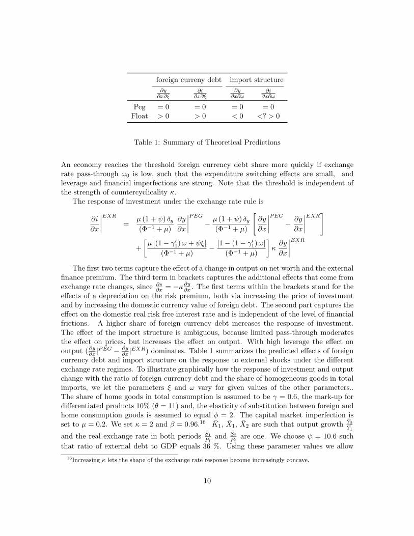
Table 1: Summary of Theoretical Predictions

An economy reaches the threshold foreign currency debt share more quickly if exchangerate pass-through ω0 is low, such that the expenditure switching effects are small, andleverage and financial imperfections are strong. Note that the threshold is independent ofthe strength of countercyclicality κ.

The response of investment under the exchange rate rule is

∂i

∂x

∣∣∣∣EXR =µ (1 + ψ) δy(Φ−1 + µ)

∂y

∂x

∣∣∣∣PEG − µ (1 + ψ) δy(Φ−1 + µ)

[∂y

∂x

∣∣∣∣PEG − ∂y

∂x

∣∣∣∣EXR]

+[µ [(1− γ′1)ω + ψξ]

(Φ−1 + µ)− [1− (1− γ′1)ω]

(Φ−1 + µ)

]κ∂y

∂x

∣∣∣∣EXRThe first two terms capture the effect of a change in output on net worth and the external

finance premium. The third term in brackets captures the additional effects that come fromexchange rate changes, since ∂s

∂x = −κ ∂y∂x . The first terms within the brackets stand for theeffects of a depreciation on the risk premium, both via increasing the price of investmentand by increasing the domestic currency value of foreign debt. The second part captures theeffect on the domestic real risk free interest rate and is independent of the level of financialfrictions. A higher share of foreign currency debt increases the response of investment.The effect of the import structure is ambiguous, because limited pass-through moderatesthe effect on prices, but increases the effect on output. With high leverage the effect onoutput ( ∂y∂x |

PEG − ∂y∂x |

EXR) dominates. Table 1 summarizes the predicted effects of foreigncurrency debt and import structure on the response to external shocks under the differentexchange rate regimes. To illustrate graphically how the response of investment and outputchange with the ratio of foreign currency debt and the share of homogeneous goods in totalimports, we let the parameters ξ and ω vary for given values of the other parameters..The share of home goods in total consumption is assumed to be γ = 0.6, the mark-up fordifferentiated products 10% (θ = 11) and, the elasticity of substitution between foreign andhome consumption goods is assumed to equal φ = 2. The capital market imperfection isset to µ = 0.2. We set κ = 2 and β = 0.96.16 K1, X1, X2 are such that output growth Y2

Y1

and the real exchange rate in both periods S1

P1and S2

P2are one. We choose ψ = 10.6 such

that ratio of external debt to GDP equals 36 %. Using these parameter values we allow16Increasing κ lets the shape of the exchange rate response become increasingly concave.

10

the share of homogeneous good imports to vary from close to zero to 50% and the foreigncurrency debt to GDP ratio from zero to 36%, holding the overall debt level constant.17

Figure (1) depicts the joint role of foreign currency debt and import structure. It showsthe difference in the fall of output to a negative external demand shock between a countrywith an exchange rate rule and a country with a peg ( ∂y∂x |

EXR − ∂y∂x |

PEG). The responseunder a peg is smaller if foreign currency debt is high and the share of homogeneous goodsis low.

Figure 1: Output response to a negative external demand shock: Difference between ex-change rate rule and peg.

3.2.3 The money rule

Results under the monetary rule (4) are similar to the exchange rate rule. The similarityis due to the fact that for an appropriately chosen κ = κ(ξ, ω) the exchange rate rule canreplicate the float. However, the money rule generates endogenously a higher depreciation, ifpass-through is lower

(∂κ∂ω < 0

). This insulates output better, through stronger expenditure

switching, if foreign debt is low. For the same reason the money rule insulates output worseif foreign debt is high and the share of differentiated goods in total imports is high, since

17There is a direct link in the model between the share of foreign debt to GDP and the parameter ξ whichis derived in the appendix.

11

now the stronger depreciation amplifies the contractionary effects. Analytical results arerelegated to the Appendix.

4 Data

We analyze the role of foreign currency debt and the import structure using a sample whichcovers yearly data for 101 countries from 1974-2007. We impose the following restrictionson the data: the sample does not include G7 countries, as the identifying assumptionon the exogeneity of external shocks may not hold for large countries. Because of dataquality concerns the study uses only countries for which we have more than five datapoints. We also discard very poor countries with a PPP adjusted GDP per capita ofless than 1000 dollars in 2007, small countries with a population of less than 1 million andobservations where the annual change in real GDP exceeds twenty percent. In line withprevious studies we only consider observations where inflation was reasonably low (belowfifty percent). Furthermore, we restrict the exchange rate regime to be in place at least oneperiod, to avoid cross-contamination due to exchange rate regime transitions. Data comefrom various sources including the IMF’s International Financial Statistics (IFS), the WorldBank’s World Development Indicators (WDI) and the Bank of International Settlements(BIS). For a detailed description see the Appendix.

Foreign Debt We employ three alternative measures. The first measure is short termexternal debt over GNI provided by the WDI. We prefer short term debt over total debt,since there is less of a roll over problem for long term debt and balance sheet effects areless immediate. As a robustness check we also report results for total external debt. Themeasure does not cover industrial countries. It is possible that part of the external debt is indomestic currency, but according to Lane and Shambaugh (2009)’s dataset almost hundredpercent of external debt (as opposed to total external liabilities) is in foreign currency. Asan alternative measure we use the claims on the domestic economy by foreign banks scaledby GDP from the BIS . The disadvantage of this dataset is that it starts only in 1983 andonly covers claims of banks from reporting countries. To reduce sensitivity to outliers weuse log(1 + debt), where debt is the corresponding debt measure expressed in percentagepoints.

Import Structure In line with findings by Campa and Goldberg (2005) we use theshare of primary commodities in a country’s total imports of goods and services to measurethe extent to which a country imports high pass-through goods. The share of primarycommodities in total imports is proxied by the sum of agricultural goods, fuels, ores andmetals over total imports as provided by the WDI. Again we use log(1 + imp), where impis the import share of raw material in percentage points.

Exchange Rate Regime The literature divides between de jure classification and defacto classification. According to Ghosh et al. (2002) the de jure classification may be

12

understood as the intention of the authority, while the de facto classifications attempts tocapture the actual behavior of the respective authority. Since we are interested in the actualconduct of exchange rate policy, our preferred exchange range classification is Levy-Yeyatiand Sturzenegger (2005)’s de facto classification (LYS) which covers the period from 1974to 2004. The authors use cluster analysis on exchange rate data and official reserves to inferthe actual exchange rate policy. The main specification uses an exchange rate dummy thattakes the value one for a peg. We will compare our results with estimates using the IMF’sde jure classification (1974-2007).

Terms of Trade We derive our terms of trade measure from various sources. The choiceof the source is guided by the length of the provided series. For most developed countries weuse the IFS terms of trade, since it is available for a long enough period. For other nationswe use UNCTAD’s terms of trade measure. If also the latter was not available for a longenough period, we made use of the constant and current export and import values availablefrom the WDI to construct the implied terms of trade.18 For a detailed description and therespective measures employed see the Appendix.

Foreign Interest Rate To measure the real foreign interest rate we use the short termreal interest rate of the reference country of relevance. The reference country is definedas in di Giovanni and Shambaugh (2008), essentially being the country by which a homecountry’s monetary policy is influenced.19 Depending on availability, the nominal shortterm rate is given by the money market or treasury bill rate and the real rate is obtainedby subtracting CPI inflation from the nominal rate in reference country.

National Accounts Real GDP and investment in local currency are taken from the WDI.

5 Model and Estimation

5.1 Empirical Model and Identification

In order to examine the conditional response to external shocks we estimate a recursiveInteracted Panel VAR of the form:

1 0 0α21

0,it 1 0α31

0,it α320,it 1

∆EXVit∆INVit∆GDPit

= µi+

L∑l=1

α11l,it 0 0α21l,it α22

l,it α23l,it

α31l,it α32

l,it α33l,it

∆EXVi,t−l∆INVi,t−l∆GDPi,t−l

+U it (16)

where EXVi,t is an external variable, either the log terms of trade or the foreign realinterest rate, GDPi,t is log real GDP, and INVi,t is log real investment for country i in period

18Apart from few exceptions, if various measures were available, they tended to be identical or at leasthighly correlated.

19The original dataset is somewhat shorter than our sample. For missing countries we used the updatedinformation provided by Reinhart and Rogoff (2004) on the partner country

13

t. Ui,t is a vector of uncorrelated iid shocks, µi is a vector of country specific intercepts andL is the number of lags. ajkl,it are deterministically varying coefficients.

We identify external shocks with a small open economy assumption. Small economies’actions have a negligible impact on goods’ world prices and the foreign interest rate. Theassumption implies that our two external variables do not depend on domestic conditionsand implies therefore strict exogeneity, which amounts to a12

l,it = a13l,it = 0 for all l. Various

other authors found that the exogeneity assumption for terms of trade generally holds fordeveloping countries (Broda, 2004; Raddatz, 2007; Loayza and Raddatz, 2007). Since weare only interested in the identification of the shock to the external variable, the describedpartial identification scheme is sufficient and the ordering of GDP and investment does notmatter.20

5.2 Interaction Terms

In order to analyze how responses vary with country characteristics, we allow for interactionterms, such that the coefficients in (16) are given by:

ajkl,it = βjkl,1 + βjkl,2 · PEGit + βjkl,3 · FCDit + βjkl,4 ·RAWit

+βjkl,5 · FCDit · PEGit + βjkl,6 ·RAWit · PEGit (17)

where PEGit is the exchange rate regime dummy, FCDit is the foreign currency debtmeasure and RAWit is the share of raw materials.

Previous studies that investigate stabilization properties of exchange rate regimes haveset βjkl,3 = βjkl,4 = βjkl,5 = βjkl,6 = 0. We start with the results for this specification for compar-ison purposes. We then look at the effects of import structure and foreign currency debtseparately by either setting βjkl,3 = βjkl,5 = 0 or βjkl,4 = βjkl,6 = 0. Finally, we look at the mostgeneral case in which all coefficients are unrestricted. While we allow the coefficients to varywith country characteristics for output and investment, we restrict the external dynamicsto be independent of country characteristics, i.e. a11

l = β11l,1 for all l. A Wald test does

not reject the null hypothesis and confirms the appropriateness of the assumption. As inevery VAR single coefficients ajkl,it cannot be interpreted. We can, however, evaluate thecoefficients at specific values and then compute impulse responses.21 While the exchangerate regime is a dummy variable, our measures of foreign currency debt and raw materialsshare are defined over a continuous range. As a benchmark we evaluate continuous variables

20Under the strict exogeneity assumption the model can equivalently be written in VARX form Yt =∑Ll=1 ClYt−l +

∑Ll=0 Dl∆EXV ARt−1 + Et and ∆EXV ARt =

∑Ll=1 Fl∆EXV ARt−l + Vt, where Yt =

(INVi,t, GDPi,t)′ and Vt, Et are reduced form error terms.

21Loayza and Raddatz (2007) apply a similar technique, but let only the coefficients on the externalvariable coefficients vary with country characteristics. The procedures leaves more degrees of freedom, but,assumes that there is only heterogeneity in the initial response, but not in the transmission. The authorsfind that less flexible labor markets and higher trade openness increase the response of a country’s GDP toterms of trade shocks.

14

at a lower (20th) percentile and a higher (80th) percentile value.22 For the exchange ratedummy the evaluation are taken at one (peg) and zero (float).

5.3 Estimation and Inference

Since the error terms are uncorrelated across equations by construction, we can estimate(16) equation by equation without loss in efficiency. In order to control for country specificintercepts we demean the data. We choose two lags following the Schwartz Criterion.23

Pesaran and Smith (1995) have shown that if there is heterogeneity in the slope coef-ficients across countries, estimates that impose a common slope are biased. The authorspropose a mean group estimator. However, using Monte Carlo simulations, Rebucci (2003)shows that in typical macro panels fixed effects panel VAR estimators outperform meangroup estimators unless slope heterogeneity is considerable. The reason is that the smallsample bias may be more detrimental to the mean group estimator than the slope hetero-geneity bias to the fixed effects estimator. Additionally, we are allowing slope coefficientsto differ with country characteristics through the interaction terms. The use of interactionterms should therefore alleviate the bias from slope heterogeneity. We are interested inthe differential slopes across exchange rate regimes conditional on country characteristics.Consequently, the mean-group estimator seems no viable alternative to us.

Since the impulse responses are a non linear function of the OLS estimates, analyticalstandard errors that rely on first order asymptotics may be inaccurate. To address thisissue we use bootstrapped standard errors as proposed by Runkle (1987) adjusted for thefact that we are dealing with a Panel and make use of interaction terms.24 The proceduremay be described in the following way. 1) Estimate (16) by OLS 2) Draw errors εi,t from anormal distribution N(0, Σ) where Σ is the estimated covariance matrix 3) use εi,t and theinitial observations of the sample and the estimates of ajkl,it to simulate recursively Yi,1.25

4) After the first period is simulated for all variables in the system interact the variableswith the interaction terms and now repeat 2 and 3 as many times as there are errors.26 5)The artificial sample, together with the interaction variables, is then used to re-estimate

22Alternatively, we can generate a dummy based on the division of country observations with high andlow external debt level and high and low raw materials share. While the continuous indicator imposes thatthe response changes in a (log) linear manner with the indicator value, the dummy implies a threshold effectrelationship. Results with dummies (not presented) underpin our findings.

23In the presence of fixed effects and lagged dependent variables, IV (or GMM) estimators are preferablefrom an asymptotic point of view if N is large and T is small. Fixed estimates are consistent for a large T.

24The programs to perform the estimation method as well as the programs to generate impulse responsesand bootstrapped confidence intervals are available from the authors upon request.

25Different to the original procedure which was not described for the Panel VAR context, we draw initialobservations panel specific and perform the simulation for each country.

26We simulated the response for each country over the entire sample length and eliminated at the end of thesimulation those observations that where missing in the original sample to maintain the same weight for eachcountry as in the initial data. Since the procedure requires the multiplication of the newly generated datawith the interaction terms in the respective period, missing observations need to be filled by interpolation.These observations will however not be part of the newly generated data as explained above.

15

the coefficients of (16) and (cumulative) IRFs are computed. 6) The procedure (step 2 to5) is repeated 500 times. The 90 % confidence interval is the minimum distance that covers90 % of the simulated estimates.27

We test in two ways whether interactions with exchange rate regime, foreign currencydebt, or raw material share have a statistically significant effect on the dynamics of thevariables. The first way, as for example done by Broda (2004), is to check with a Wald testwhether the interaction terms in the recursive VAR model are jointly significant. Such aprocedure tests whether the interaction terms can explain a statistically significant fractionof the overall variation in the dependent variables. The test allows no direct inferenceon whether there are significant differences in the response to a specific shock, at a specifictime horizon. To address this question we compare (cumulative) impulse response functionspairwise with a t-test.

t =IRF (PEG1, RAW1, FCD1)t − IRF (PEG2, RAW2, FCD2)t

σ(IRF1,t − IRF2,t)(18)

The null is that the response of two countries with given exchange rate regime, foreigncurrency debt, and import structure to a shock after t years is equal. The standard devia-tion of the difference between the two responses σ(IRF1,t − IRF2,t) is estimated from thebootstrap sample. 28

6 Results

6.1 Floats versus Pegs

As a first step we contrast the response of output and investment under different exchangerate regimes, irrespective of the degree of foreign currency debt and of the import structure.Figure 2 shows the cumulative response of output and investment to a negative 10% termsof trade shock using the LYS exchange rate classification. With a peg output falls by about1 % in two years, whereas under a float output falls by about 0.6 %. The result is thereforein line with the classic argument that flexible exchange rates are better suited to absorbreal shocks and confirms previous empirical studies by Edwards and Levy Yeyati (2005)and Broda (2004). According to a Wald test the interaction terms are jointly significant. At-test, however, finds the difference in the response to terms of trade shocks not statisticallysignificant at any horizon. The responses of investment are similar and not statisticallysignificantly different. Under a float the response is even slightly stronger.

Table 2 presents the results for alternative specifications. With the IMF’s de jure ex-change rate regime classification, we again find evidence that the output response under afloat is smaller. The results for a shock to the foreign interest rate are similar to those for

27Kilian (1998) showed that the IRFs may still suffer from small sample bias. We find no evidence of sucha bias in our results, since the mean of the bootstrapped responses tends to coincide with the point estimate,the difference between the two being the bias correction proposed by Kilian.

28An alternative to the t-test is to look directly at the empirical distribution of impulse response differencesand evaluate which fraction lies above zero. Such a procedure gives very similar results.

16

Figure 2: Impulse Responses for an initial 10% Terms of Trade Shock under LYS classifi-cation

Output Investment1st year 2nd year 5th year 1st year 2nd year 5th year

10% ToT Shock, LYSFix -0.39 -0.98 -1.28 -1.21 -2.62 -3.28Float -0.37 -0.66 -0.8 -1.38 -2.88 -3.45Wald Test 0.0110% ToT Shock, IMFFix -0.26 -0.73∗ -1.22∗ -1.46∗∗∗ -2.92∗∗∗ -4.13∗∗∗

Float -0.08 -0.35 -0.64 -0.02 -0.64 -1.4Wald Test 0.00100bps foreign interest rate shock, LYSFix -0.01 -0.27 -0.51∗ -0.03 -0.74 -1.87Float 0.07 -0.02 -0.11 0.36 -0.49 -1.02Wald Test 0.00Stars (*) stand for the t test statistic that compares pegs and floats. ***,**,* indicate the t-statistic liesbelow the 2.5%, 5%, 10% percentile and the response is therefore statistically significantly lower than forits counterpart. ”Wald Test” reports the p-value of the test for the joint significance of all interactionterms.

Table 2: Output and Investment Response to External Shock, Conditional on the ExchangeRate Regime

17

the terms of trade shock. After a 100 bps shock output falls by about 0.4 % under a peg,whereas output under a float remains virtually unchanged.

6.2 The Role of Foreign Currency Debt

We proceed by looking at the response of output under different exchange rate regimesconditional on the degree of foreign currency indebtedness (Figure 3). Flexible exchangerates insulate better from terms of trade shocks if foreign debt is low: In the second year theoutput response under a flexible exchange rate is insignificant, while output has declinedby more than one percent under a fixed exchange rate. The finding is reversed for highforeign debt: Under a peg the output response is of similar magnitude as under the lowdebt counterpart. The response under a float, however, is substantially stronger than inthe low debt case and output declines by about 1.1 percent. A Wald test confirms thejoint significance of all interaction terms. Pairwise t-tests find a significant difference in theoutput response between pegs and floats when foreign currency debt is low, but not if it ishigh. Under a float, there is also a significantly stronger output response with high foreigndebt compared to low foreign debt.

The balance sheet effects theory suggests that the main reason for the difference betweenthe output response of a float with high and low foreign currency debt is investment. Withhigh foreign currency debt, a depreciation reduces firm’s net worth more, which leads totighter credit conditions and less investment. Figure 3 affirms the importance of investment,although the confidence bands are rather wide. With low foreign currency debt, investmentbehaves similarly under both exchange rate regimes. It declines by about 1.5 percent withintwo year. With high foreign currency debt, the investment response under a float is stronger:investment declines by 4.3 percent under a float compared to 3 percent under a peg.

With the estimates at hand, we can simulate the accumulated response of output toterms of trade shocks across various degrees of external indebtedness and define zones forwhich floats insulate output better from terms of trade shocks than pegs. Figure 4 showsthe accumulated response of output after two years for varying degrees of indebtedness.29

The response of output to the shock under fixed regimes shows no particular sensitivityto the extent of foreign currency debt, but under a float the response rises with higherdebt. According to the estimates output responds less under a float up to a short termexternal debt to GNI ratio of 10 percent. Roughly 25 percent of all observations lie abovethis threshold. The investment response under a float is stronger for most levels of foreigncurrency debt and increases also faster with debt compared to a peg. The higher sensitivityof investment under a float is consistent with the idea that balance sheet effects play animportant role.

Table 3 reports alternative specifications. Our results for output and investment withtotal external debt instead of short term debt are quantitatively similar, but not alwayssignificant because of higher parameter uncertainty, consistent with the idea there is less ofa rolling over problem for long term debt. Using claims of foreign banks instead gives again

29The conclusion is similar if we use other horizons.

18

Figure 3: Impulse Responses for a negative 10% Terms of Trade Shock under LYS classifi-cation

similar results. Using the IMF’s de jure exchange rate regime classification also confirms ourfindings. The results for responses to a foreign interest rate shock are a bit less clear. Thereare no statistically significant differences in pairwise comparison of impulse responses, evenif a Wald test finds the interaction terms involving foreign debt to be jointly significant.Both with high and low debt, the response under a peg is slightly stronger. With highforeign debt the response of output and investment is again stronger, consistent with theinterpretation that balance sheet effects become more important.

6.3 The Role of Import Structure

In a next step we attempt to shed some light on the role of import structure in the trans-mission of shocks. A Wald test indicates joint significance of all interaction terms. Figure5 shows the response of output and investment in countries with a high and a low shareof raw materials in total imports. With a high share of raw materials and therefore highpass-through, flexible exchange rates shield output better from terms of trade shocks. Incountries that have a high raw material share and maintain a peg output falls by about 1.5percent in two years, while it falls only by a bit more than 0.5% under a float. For countrieswith low pass-through the picture is reversed. Under a peg output falls by 0.5% and undera float it falls by about 1.5%. The differences are statistically significant in both cases. Apotential explanation for the higher response under a float are balance sheet effects that canno longer by compensated with expenditure switching. The explanation is consistent withthe response of investment. For observations with a low raw material share, investment falls

19

Output Investment1st year 2nd year 5th year 1st year 2nd year 5th year

10% ToT Shock, LYS, Short term ext. debtFix-HFCD -0.32 -0.94 -1.25 -1.03 -3.14 -3.52Float-HFCD -0.42 -1.1++ -1.2+ -1.51 -4.3+ -4.82Fix-LFCD -0.54 -1.04∗∗∗ -1.2∗∗ -1.2 -1.43 -2.18Float-LFCD -0.23 -0.04 -0.1 -1.02 -1.57 -2.18Wald Test 0.00 0.00 0.0310% ToT Shock, IMF, Short term ext. debtFix-HFCD -0.24 -0.74 -1.02 -1.41 -3.39 -3.85Float-HFCD -0.38+++ -1.00+++ -1.55+++ -0.87++ -3.2+++ -4.67+++

Fix-LFCD -0.29∗∗ -0.69∗∗∗ -1.19∗∗∗ -1.73∗∗∗ -2.81∗∗∗ -4.08∗∗∗

Float-LFCD 0.13 0.28 0.40 0.87 2.07 1.38Wald Test 0.00 0.00 0.0010% ToT Shock, LYS, total ext. debtFix-HFCD -0.18 -0.9 -1.26 -0.67 -2.66 -3.47Float-HFCD -0.31 -0.66 -0.8 -1.32 -3.49 -3.83Fix-LFCD -0.42 -1.02 -1.2 -1.44 -2.79 -2.92Float-LFCD -0.31 -0.33 -0.44 -1.09 -1.51 -2.53Wald Test 0.00 0.00 0.2610% ToT Shock, LYS, BISFix-HFCD 0.08 -0.93 -0.86 -0.31 -2.85+ -1.9Float-HFCD -0.4∗ -1.05 -1.15 -1.12 -3.62 -3.38Fix-LFCD -0.34+++ -0.74 -0.94 -0.51 -1.2 -2.03Float-LFCD -0.57 -0.59 -0.79 -1.43 -2.4 -2.5Wald Test 0.00 0.00 0.00100bps foreign interest rate shock, LYS, Short term ext. debtFix-HFCD -0.1+ -0.39 -0.73 -0.74∗∗++ -0.79 -2.86++

Float-HFCD 0.08 -0.15 -0.35 0.55 -0.8 -1.9Fix-LFCD 0.1 -0.1 -0.27 0.42 -0.24 -0.83Float-LFCD 0.11 0.15 0.09 0.06 -0.58 -0.78Wald Test 0 0 0.29HFCD and LFCD stand for High and Low Foreign Currency Debt. Stars (*) stand for the t test statisticthat compares pegs and floats with the same level of FCD. Crosses (+) stand for t statistic that comparesthe response under the same regime for HFCD and LFCD. ***(+++),**(++),*(+) indicate the t-statisticlies below the 2.5%, 5%, 10% percentile and the response is therefore statistically significantly lower thanfor its counterpart. The first, second, and third column of ”‘Wald Test” report the p value of tests for thejoint significance of all interaction terms, the joint significance of all interaction terms that involve FCDor FCD*PEG, the joint significance of all interaction terms that involve FCD*PEG.

Table 3: Output and Investment Response to External Shock, Conditional on Short TermExternal Debt and Exchange Rate Regime

20

Figure 4: Cumulative Response of Output and Investment to a 10% ToT Shock in thesecond year as a function of foreign currency debt

by about 4 % under a float and only by about 2% under a peg.As with foreign currency we can investigate how the respective exchange rate regime

performs by evaluating the cumulative output response at different levels of our importstructure measure. Figure 6 shows the accumulated response of output in the second yearfor varying shares of raw materials on total imports. As expected we find that the insula-tion ability of the float increases with the raw material share, when expenditure switchingdominates the balance sheet effect. For fixed regimes on the other hand, the response ofoutput to terms of trade shocks increases with the pass-through. The response of pegs andfloats intersect at a raw material share of 14 %. Roughly 55 % of the observations lie belowthe threshold.

If we use the de jure exchange rate classification a similar picture emerges, but thedifferences in pairwise comparison of impulse responses are smaller and not statisticallysignificant (Table 4). The result is in line with our argument that actual exchange ratepolicy is more important than declared policy. A Wald test finds joint significance of allinteraction terms. If we analyze the response of output to a foreign interest rate shock, weagain confirm the that flexible exchange rate insulates output only significantly better whenraw material imports are relatively large.

6.4 The Joint Role of Foreign Currency Debt and Import Structure

Our results so far have shown that there is no empirical evidence that output respondsgenerally less to a real shock under a float. Consistent with theoretical underpinnings wefind the insulation properties of floats vanish for import structures associated with low

21

Figure 5: Impulse Responses for a Negative 10% Terms of Trade Shock under LYS classifi-cation

Figure 6: Cumulative Response of Output and Investment to a 10% ToT Shock in thesecond year as a function of raw material share in total imports

22

Output Investment1st year 2nd year 5th year 1st year 2nd year 5th year

10% ToT Shock, LYS, Raw Material ShareFix-HRAW -0.76+++ -1.52∗∗+++ -2.4∗+++ -2.8+++ -3.09 -4.56Float-HRAW -0.46 -0.61 -1.08 -1.78 -3.27 -4.09Fix-LRAW -0.12 -0.57 -0.9 -0.46 -2.12 -2.33Float-LRAW -0.64∗∗ -1.49∗∗++ -1.47 -2.21∗ -4.14 -4.07Wald Test 0 0 0.0110% ToT Shock, IMF, Raw Material ShareFix-HRAW -0.31 -0.87 -1.58 -2.84∗+++ -3.51 -4.87Float-HRAW -0.43 -0.44 -0.92 -1.49 -2.17 -3.41Fix-LRAW -0.12 -0.65 -1.45 -0.79 -2.8 -4.34Float-LRAW -0.2 -0.73 -0.81 -0.98 -1.63 -2.43Wald Test 0 0 0100 bps foreign interest rate shock, LYS, Raw Material ShareFix-HRAW -0.26∗++ -0.73∗++ -1.31∗∗+++ -0.43 -1.36 -3.17∗

Float-HRAW 0+ -0.21 -0.37 0.58 -0.6 -0.89Fix-LRAW 0.04∗ -0.17 -0.29 -0.11∗∗ -0.76 -1.56Float-LRAW 0.3 0.14 -0.2 1.1 0.3 -1.59Wald Test 0 0 0.17HRAW and LRAW stand for High and Low share of raw materials in total imports. Stars (*) stand for the ttest statistic that compares pegs and floats with the same level of FCD. Crosses (+) stand for t statistic thatcompares the response under the same regime for HRAW and LRAW. ***(+++),**(++),*(+) indicate thet-statistic lies below the 2.5%, 5%, 10% percentile and the response is therefore statistically significantlylower than for its counterpart. The first, second, and third column of ”‘Wald Test” report the p value oftests for the joint significance of all interaction terms, the joint significance of all interaction terms thatinvolve RAW or RAW*PEG, the joint significance of all interaction terms that involve FCD*PEG.

Table 4: Output and Investment Response to External Shock, Conditional on Import Struc-ture and Exchange Rate Regime

23

levels of pass-through and for high levels of foreign currency debt. We now turn to thecomplete specification and let the responses be a function of the exchange rate regime,foreign currency debt, and import structure.30

We take the value of the cumulated response of output within two years as a benchmarkand simulate this response along the grid of possible constellations of foreign currencydebt and import structures for fixed regimes and flexible regimes. Then we subtract thecorresponding value of the peg from the float. A value below zero implies the response ofoutput under the float is stronger. The lower the value the stronger is the relative responseunder a float. Figure 7 confirm the previous findings and resembles the shape of Figure 1from the theoretical model. The output response under a float is weaker if the raw materialshare is high and foreign debt is low. The picture weakens and finally reverses if either theraw material share is low or foreign debt is high.

Figure 7: Output response to a negative 10 % terms of trade shock in the second year:Difference between float and peg.

30Clearly this leads to a significant loss in degrees of freedom, given that we employ two lags and work withthree variables. Nevertheless, results are in line with the former findings and confidence intervals remainreasonably tight. To save space results are not reported but available from the authors.

24

7 Conclusion

Even though we are equipped with a battery of theoretical models about the implications ofthe choice of the exchange rate regime under various rigidities and institutional frameworks,empirical work has lagged behind. Previous studies have either not distinguished betweenthe various shocks that hit the economy or not accounted for differences in the frictionsor the economic structure that affect the response to shocks. In the present study we syn-thesize theoretical considerations in a stylized three equation model to analyze how limitedpass-through and foreign currency debt affect the buffer property of a flexible exchangerate. We show that flexible exchange rates do not necessarily shield output better from realexternal shocks than pegs. With high foreign currency debt and low pass-through contrac-tionary balance sheet effects dominate expansionary expenditure switching effects. Usingan Interacted Panel VAR for a large sample of countries we test and confirm the predictionsof the extended IS-LM-BP model by allowing the response of output and investment toan external shock vary with the exchange rate regime, the foreign currency debt and theimport structure.

Our analysis focuses on how the exchange rate regime affects macroeconomic adjustmentto real external shocks. Policy makers will also care about other aspects when choosing anexchange rate regime, such as its effects on inflation, trade volumes, long term growth or onthe likelihood of financial crises. Our results suggest that ceteris paribus the case for a floatweakens if a country has high foreign currency debt and imports mainly low pass-throughgoods.

References

Baxter, Marianne, and Alan C. Stockman (1989) ‘Business cycles and the exchange-rateregime : Some international evidence.’ Journal of Monetary Economics 23(3), 377–400

Bebczuk, Ricardo N., Ugo Panizza, and Arturo Galindo (2006) ‘An evaluation of the con-tractionary devaluation hypothesis.’ RES Working Papers 4486, Inter-American Devel-opment Bank, Research Department, July

Bernanke, Ben, Mark Gertler, and Simon Gilchrist (1998) ‘The financial accelerator in aquantitative business cycle framework.’ NBER Working Papers 6455, National Bureau ofEconomic Research, Inc, March

Broda, Christian (2004) ‘Terms of trade and exchange rate regimes in developing countries.’Journal of International Economics 63(1), 31–58

Broda, Christian, and Cedric Tille (2003) ‘Coping with terms-of-trade shocks in developingcountries.’ Current Issues in Economics and Finance

Campa, Jos Manuel, and Linda S. Goldberg (2005) ‘Exchange rate pass-through into importprices.’ The Review of Economics and Statistics 87(4), 679–690

25

Cavallo, Michele, Kate Kisselev, Fabrizio Perri, and Nouriel Roubini (2004) ‘Exchange rateovershooting and the costs of floating.’ Proceedings

Cespedes, Luis Felipe, Roberto Chang, and Andres Velasco (2004) ‘Balance sheets andexchange rate policy.’ American Economic Review 94(4), 1183–1193

Cespedes, Luis Felipe, Roberto Chang, and Andrs Velasco (2003) ‘Must original sin causemacroeconomic damnation?’ Working Papers Central Bank of Chile 234, Central Bankof Chile, October

Choi, Woon Gyu, and David Cook (2004) ‘Liability dollarization and the bank balancesheet channel.’ Journal of International Economics 64(2), 247–275

Cook, David (2004) ‘Monetary policy in emerging markets: Can liability dollarization ex-plain contractionary devaluations?’ Journal of Monetary Economics 51(6), 1155–1181

Devereux, Michael B., and Charles Engel (2003) ‘Monetary policy in the open econ-omy revisited: Price setting and exchange-rate flexibility.’ Review of Economic Studies70(4), 765–783

Devereux, Michael B., Philip R. Lane, and Juanyi Xu (2006) ‘Exchange rates and monetarypolicy in emerging market economies.’ Economic Journal 116(511), 478–506

di Giovanni, Julian, and Jay C. Shambaugh (2008) ‘The impact of foreign interest rates onthe economy: The role of the exchange rate regime.’ Journal of International Economics74(2), 341–361

Edwards, Sebastian, and Eduardo Levy Yeyati (2005) ‘Flexible exchange rates as shockabsorbers.’ European Economic Review 49(8), 2079–2105

Eichengreen, Barry, Ricardo Hausmann, and Ugo Panizza (2003) ‘Currency mismatches,debt intolerance and original sin: Why they are not the same and why it matters.’ NBERWorking Papers 10036, National Bureau of Economic Research, Inc, October

Fleming, John M. (1962) ‘Domestic financial policies under fixed and under. floating ex-change rates.’ IMF StaffPapers 9, IMF StaffPapers, November

Flood, Robert P., and Andrew K. Rose (1995) ‘Fixing exchange rates a virtual quest forfundamentals.’ Journal of Monetary Economics 36(1), 3–37

Friedman, Milton (1953) ‘The case for flexible exchange ratess.’ Technical Report

Galindo, Arturo, Ugo Panizza, and Fabio Schiantarelli (2003) ‘Debt composition and bal-ance sheet effects of currency depreciation: a summary of the micro evidence.’ EmergingMarkets Review 4(4), 330–339

26

Gertler, Mark, Simon Gilchrist, and Fabio M. Natalucci (2007) ‘External constraints onmonetary policy and the financial accelerator.’ Journal of Money, Credit and Banking39(2-3), 295–330

Ghosh, A.R., A.M. Gulde, and H.C. Wolf (2002) Exchange Rate Regimes: Choices andConsequences (MIT Press)

Ghosh, Atish R., Anne-Marie Gulde, Jonathan D. Ostry, and Holger C. Wolf (1997) ‘Doesthe nominal exchange rate regime matter?’ NBER Working Papers 5874, National Bureauof Economic Research, Inc, January

Hausmann, Ricardo, Ugo Panizza, and Ernesto Stein (2001) ‘Why do countries float theway they float?’ Journal of Development Economics 66(2), 387–414

Hoffmann, Mathias (2007) ‘Fixed versus flexible exchange rates: Evidence from developingcountries.’ Economica 74(295), 425–449

Kehoe, Timothy J., and Kim J. Ruhl (2008) ‘Are shocks to the terms of trade shocks toproductivity?’ Review of Economic Dynamics 11(4), 804–819

Kilian, Lutz (1998) ‘Small-sample confidence intervals for impulse response functions.’ TheReview of Economics and Statistics 80(2), 218–230

Krugman, Paul (1986) ‘Pricing to market when the exchange rate changes.’ NBER WorkingPapers 1926, National Bureau of Economic Research, Inc, May

Lane, Philip, and Jay Shambaugh (2009) ‘Financial exchange rates and international cur-rency exposures.’ American Economic Review

Levy-Yeyati, Eduardo, and Federico Sturzenegger (2005) ‘Classifying exchange rate regimes:Deeds vs. words.’ European Economic Review 49(6), 1603–1635

Loayza, Norman, and Claudio E. Raddatz (2007) ‘The structural determinants of externalvulnerability.’ The World Bank Economic Review 21(3), 359–387

Miniane, Jacques, and John H. Rogers (2007) ‘Capital controls and the international trans-mission of u.s. money shocks.’ Journal of Money, Credit and Banking 39(5), 1003–1035

Mundell, Robert A. (1961) ‘A theory of optimum currency areas.’ American EconomicReview (51), 657–665

Mussa, Michael (1986) ‘Nominal exchange rate regimes and the behavior of real exchangerates: Evidence and implications.’ Carnegie-Rochester Conference Series on Public Policy25(1), 117–214

Pesaran, M. Hashem, and Ron Smith (1995) ‘Estimating long-run relationships from dy-namic heterogeneous panels.’ Journal of Econometrics 68(1), 79–113

27

Raddatz, Claudio (2007) ‘Are external shocks responsible for the instability of output inlow-income countries?’ Journal of Development Economics 84(1), 155–187

Ramcharan, Rodney (2007) ‘Does the exchange rate regime matter for real shocks? evidencefrom windstorms and earthquakes.’ Journal of International Economics 73(1), 31–47

Rebucci, Alessandro (2003) ‘On the heterogeneity bias of pooled estimators in stationaryvar specifications.’ IMF Working Papers 03/73, International Monetary Fund, April

Reinhart, Carmen M., and Kenneth S. Rogoff (2004) ‘The modern history of exchange ratearrangements: A reinterpretation.’ The Quarterly Journal of Economics 119(1), 1–48

Runkle, David E. (1987) ‘Vector autoregressions and reality.’ Staff Report 107, FederalReserve Bank of Minneapolis

Tovar, Camilo E (2005) ‘The mechanics of devaluations and the output response in a dsgemodel: how relevant is the balance sheet effect?’ BIS Working Papers 192, Bank forInternational Settlements, November

28

A Derivation of the Model

The steps follow closely Cespedes et al. (2003) and are therefore brief.

A.1 IS Curve

Using the pricing rule and the fact that workers consume all income, the log linear versionof the market clearing condition in period 2 (6) is

y2 = κ [(φ− 1) (q2 − p2) + y2] + (1− κ) (s2 − p2) (19)

where κ = γ (1− α)(1− θ−1

) (P2

Q2

)1−φ.

The log linearized version of the price index in period 2 is

q2 =(1− γ′2

)s2 + γ′2p2, (20)

where γ′2 = 1−(1− γ)(S2

Q2

)(1−φ).31 Using equations (19) and (20) gives output as a function

of the real exchange rate

y2 = Ξ (s2 − p2) , (21)

where Ξ = [1 + (φ− 1) (1− γ′2) κ/ (1− κ)] ≥ 1.Using (21) in the log linear version of (1) the consumption level in period 2 is given by

c2 = y2 − (q2 − p2) (22)

Since no shock occurs in the second period l = 0, output deviations in the second periodare driven by investment.

y2 = αi1 (23)

The linearized version of the market clearing condition in the first period (5) is

τy1 + (1− τ) [c1 + φq1] = λ [i1 + φq1] + (1− λ) (s1 + x1) (24)

where τ = 1

1−γ(P1Q1

)−φ(1−α)(1−θ−1)

> 1 and λ =γ(P1Q1

)−φI1

γ(PQ

)−φI1+

S1P1X1

< 1.

Since capital is predetermined and wages are preset we have from the workers budgetconstraint ( 1).

q1 + c1 =y1

1− α(25)

The price index in period 1 is

q1 =(1− γ′1

)ωs1 (26)

31The share of differentiated goods plays no role, because no shocks occur in the second period and foreignproducers of differentiated goods take shocks in the initial period into account.

29

where γ′1 = 1− (1− γ)(S1

Q1

)(1−φ). Combining (24), (25) and (26) gives the IS curve

y1

(1− τα1− α

)= λi1 + (1− λ)x1 +

{(1− λ) + λ

(1− γ′1

)ω

[φ+

(τ − 1)λ

(φ− 1)]}

s1

A.2 LM: Money Demand

From the consumer maximization problem we have that the log linear version of moneydemand in period one and two is respectively

ζ (m1 − q1) + (1− ζ) (c2 + q2 − q1) = c1 (27)ζ (m2 − q2) = c2 (28)

where ζ = 1 − βQ1C1/Q2C2 , which is assumed to be positive. Combining the aboveequation with (22), (23), (25), and (26) gives

m1 =1ζ

y1

1− α− (1− ζ)

ζαi1 −

(1− ζ)ζ

p2

A.3 BP: Entrepreneurs

The return on investment must satisfy the arbitrage condition with foreign returns adjustedby a risk premium

r2 − q1 − p2 = ρ+ η1 + (s2 − p2)− s1 (29)

The marginal product of capital is given by r2 − p2 = −i1 (1− α). Using this result, (26)and (21) gives:

i1Φ−1 = − (ρ+ η1) + [1− (1− γ)ω] s1 (30)

where Φ = ΞΞ(1−α)+α ≥ 1.

The log linear version of the risk premium is

η1 = µ [q1 + i1 − n1] (31)

The log linear version of net worth equation

n1 = (1 + ψ) δyy1 − ψξs1 (32)

where δy = θ−1[1− (1− α)

(1− θ−1

)]−1.

Using (31) in (32) gives:

η = µ {i− δyy + [(1− γ)ω + δs] s}

which can be used in (30) to derive the BP schedule:

i1(Φ−1 + µ

)= −ρ+ µ (1 + ψ) δyy1 − µ [(1− γ)ω + ψξ] s1 + [1− (1− γ)ω] s1

30

Note also that there is a direct link between ψ and the share of debt to GDP. To seethis note that

P1N1

P1Y1=

R1K1 + Π1

P1Y1− S1D

∗1

P1Y1− D1

P1Y1

=P1Y1 − W1L1

P1Y1− S1D

∗1

P1Y1− D1

P1Y1

Using the standard pricing rule W1LP1Y1

= (1− α) θ−1θ this implies

P1N1

P1Y1= 1− (1− α)

(1− θ−1

)− S1D

∗1 + D1

P1Y1

Varying the share of foreign currency debt to GDP ratio(S1D

∗1/P1Y1

)gives the implied(

P1N1/P1Y1

)ratio (for a given level of domestic debt D1/P1Y1), which in turn allows

to determine the total debt to net worth ratio ψ = (S1D∗1 +D1) /P1N1 and the implied

foreign currency share in total debt ratio ξ = S1D∗1/(S1D

∗1 + D1

). Consider the standard

parametrization θ = 11 and α = 1/3 then we have for a domestic debt to GDP ratio of 12%and a foreign debt to GDP ratio of 24% that P1N1/P1Y1 = 0.04 and ψ = 9 and ξ = 2/3.

B Solving the system

In the following we use equations (7), (8) and (9) and combine them with the monetarypolicy - peg, exchange rate rule or float - to determine the respective implied response ofoutput and investment to an external demand shock.

B.1 The Peg

Under a peg monetary policy is given by s = 0. This simplifies the system which determinesoutput and investment to the following two equations:

y

(1− α1− τα

)= λi+ (1− λ)x (33)

i(Φ−1 + µ

)= −ρ+ µ (1 + ψ) δyy (34)

The impact of a terms of trade shock on output and investment is determined by solvingthe system which yields equation (10) and (11) in the text:

∂y

∂x=[

1− α(1− λ) (1− τα)

− λµ (1 + ψ) δy(1− λ) (Φ−1 + µ)

]−1

i =∂y

∂x

µ (1 + ψ) δy(Φ−1 + µ)

31

B.2 The Exchange Rate Rule

Under the exchange rate rule we have that s = −κy , which we use to substitute out forthe exchange rate yielding the following two equation system.

y

(1− α1− τα

)= λi+ (1− λ)x− [(1− λ) + ωλg]κy (35)

i =µ (1 + ψ) δy + µ [(1− γ′1)ω + ψξ]κ− [1− (1− γ′1)ω]κ

(Φ−1 + µ)y

Combining the two equations we can solve for output, which yields:

∂y

∂x= χ

[(1−α)(Φ−1+µ)

(1−τα) − µλ (1 + ψ) δy +(Φ−1 + µ

)ωλgκ− λ (1− γ′1)ωκ

−λµψξκ− λµ (1− γ′1)ωκ+[(1− λ)

(Φ−1 + µ

)+ λ

]κ

]−1

where χ = (1− λ)(Φ−1 + µ

). This is equation (12) in the text. Investment is given by

∂i

∂x=µ (1 + ψ) δy + µ [(1− γ′1)ω + ψξ]κ− [1− (1− γ′1)ω]κ

(Φ−1 + µ)∂y

∂x

The derivative with respect to ω is

∂i

∂x∂ω

∣∣∣∣EXR =µ (1 + ψ) δy(Φ−1 + µ)

∂y

∂x∂ω

∣∣∣∣EXR +[µ [(1− γ′)ω + ψξ]

(Φ−1 + µ)− [1− (1− γ′)ω]

(Φ−1 + µ)

]κ

∂y

∂x∂ω

∣∣∣∣EXR+µ [(1− γ′)] + (1− γ′)

(Φ−1 + µ)κ∂y

∂x

∣∣∣∣EXRFor µ > 0 the first term is unambiguously negative, the third term is unambiguously

positive, and the sign of the second term is ambiguous, which makes the sign of the overallexpression ambiguous.

B.2.1 Evaluating the response of ∂2y/∂x∂ω

To proof that the derivative ∂2y/∂x∂ω < 0 we proceed in two steps. First, we show thatfor µ = 0 we obtain a negative value for the derivative. Second, we show that the value iscontinuously decreasing in µ. Thus, the derivative can only be positive if µ < 0 which isnot in the possible set of values.

Consider the term in brackets in (14) . Substituting out g (φ) = (1− γ′1) [φ+ (φ− 1) (τ − 1) /λ]we can write.

(1 + µ)(Φ−1 + µ)

(1− γ′1

)− g =

(1− γ′1

){ (1 + µ)(Φ−1 + µ)

− [φ+ (φ− 1) (τ − 1) /λ]}, (36)

since (1− γ′1) > 0, it is sufficient to determine the sign of the term in curly brackets.

32

Now consider µ = 0. Since Φ = ΞΞ(1−α)+α > 1, multiplying all terms with Φ−1 will not

change the sign of term in curly brackets and we have:

1− α[φ+ (φ− 1) τ−1

λ

]Ξ

− (1− α)[φ+ (φ− 1)

τ − 1λ

]≤ 0

The inequality follows form the fact that for φ = 1 , we have Ξ = 1 and thus the entire term

is zero. For any value of φ > 1 the term is negative since [φ+(φ−1) τ−1λ ]

Ξ and[φ+ (φ− 1) τ−1

λ

]are increasing in φ.The last step is to show that the (36) is decreasing in µ. This is quickly

seen by recognizing that g and γ′1 are independent of µ and∂[(1+µ)/(Φ−1+µ)]

∂µ < 0 sinceΦ−1 < 1 for φ > 1.

B.2.2 The Money Rule

The constant money rule implies for the LM that

i =1

(1− ζ) (1− α)αy (37)

Using this result in the BP yields:

s = −κ (ω, ξ) y (38)

where κ (ω, ξ) = B [(1 + µ) (1− γ′)ω + µψξ − 1]−1 andB =(Φ−1 + µ

)[(1− ζ) (1− α)α]−1−

µ (1 + ψ) δy. The system is completed by the IS equation (35). Using in the exchange rate

rule the particular value κ = κ (ω, ξ) gives ∂y∂x

∣∣∣CMRand demonstrates the equivalence be-

tween the constant money rule and the exchange rate rule if κ adjusts endogenously toreestablish the equilibrium in the money market. The solution for investment under theconstant money rule reads:

∂i

∂x

∣∣∣∣CMR

=1

(1− ζ) (1− α)α∂y

∂x

∣∣∣∣CMR

33

C Data Sources

In the following we describe the indices and transformations which we applied to the data:

Exchange Rate Regimes: The de jure classification needed to be unified since it is based onthe changing IMF Annual Report on Exchange Arrangements and Exchange Restric-tions (AREAER). The classification went through four distinct phases of change. It ispossible to group the countries consistently into 3 broad categories, floating, interme-diate and fixed regimes. The original IMF classification is coded in four taxonomies:Taxonomy 1 from 1975 to 1976 includes: ”Pegged to a single currency” (1), ”Peggedto a composite (including the SDR)” (2), ”Floating - adjusted according to a set ofindicators” (3), ”Floating - common margins” (4) and ”Floating - independently”(5). Taxonomy 2 from 1977 to 1981 distinguishes: ”Pegged to a single currency” (1),”Pegged to a composite (including the SDR)” (2), ”Adjusted according to a set ofindicators” (3), ”Cooperative exchange arrangements” (4), ”Other” (5). Taxonomy 3ranges from 1982 to 1998 with: ”Pegged to a single currency” (1), ”Pegged to a com-posite (including the SDR)” (2), ”Flexibility limited vis-a-vis a single currency” (3),”Flexibility limited vis-a-vis a cooperative arrangement” (4), ”Adjusted according toa set of indicators” (5), ”Other managed floating” (6) and ”Independently floating”(7). Taxonomy 4 from 1998 to today: ”Exchange arrangement with no separate legaltender” (1), ”Currency board arrangement” (2), ”Conventional pegged arrangement”(3), ”Conventional peg to a basket” (3,5), ”Pegged exchange rate within horizontalbands” (4), ”Crawling peg” (5), ”Crawling band” (5), ”Managed floating (7) and”Independently floating” (8). The ”harmonized” IMF de jure classification that isemployed here is based on the following mapping:

New Former ClassificationsUnified Tax 1 Tax 2 Tax 3 Tax 4Peg 1,2 1,2 1,2 1,2,3,3,5Interm 3,4 3,4,5* 3,4,5,6 4,5,6,7Float 5 5* 7 8

Import Structure: The share of primary commodities in total imports is proxied by thesum of agricultural goods, fuels, ores and metals over total imports. We use the dataon shares of imports according to various product groups as provided by the WDI.We rescale the shares in terms of total imports of goods and services rather thanmerchandise imports. Hence, the import structure measure is:

PASS = log(

1 +∑raw material imports

total imports∗ 100

)where we take the log to limit the role of outliers.

Terms of Trade: Despite the fact that the IFS, the WDI (net barter terms of trade) andUNCTAD provide terms of trade data, they are not covering the entire sample. To

34

enlarge the sample we constructed a proxy based on current and constant values ofexport and import data. In particular we used exports and imports in constant USdollars and current US dollars to construct the TOT proxy

ToT =EXPORTScurEXPORTSconIMPORTScurIMPORTScon

which we scale to the base year 2000 to make the measure comparable to the IFSdata.32 Our final terms of trade measure uses this measure, if the other measures donot provide sufficiently large series. As a check we use consistently our ToT proxy forall countries.

The choice for the indicator employed follows the length of the available series using ifpossible IFS then UNCTAD and then the implied terms of trade from the WDI constantand current value of exports and imports. Whenever a country’s terms of trade remainsunchanged for three consecutive years or has breaks in the series an alternative classificationis preferred. The respective countries in the sample and the term of trade measure used isgiven below:

32Other authors have used this approach before. See for instance Loayza and Raddatz (2007) or Kehoeand Ruhl (2008)

35

Albania Ghana PanamaAlgeria Greece1 Papua New Guinea

Argentina Guatemala Paraguay2

Australia1 Guinea2 PeruAustria Honduras Philippines

Azerbaijan Hong Kong, China1 Poland1

Bangladesh Hungary PortugalBelarus India Romania

Belgium Indonesia Russian FederationBenin Iran, Islamic Rep. Saudi Arabia 2

Bolivia Ireland1 SenegalBotswana Israel1 Singapore 1

Brazil Jordan1 Slovak RepublicBulgaria Kazakhstan Slovenia

Burkina Faso Kenya South AfricaCambodia Korea, Rep. SpainCameroon Kuwait Sri Lanka1

Chad Kyrgyz Republic Sweden1

Chile Latvia SwitzerlandChina Lebanon Syrian Arab Republic

Colombia Lithuania TajikistanCosta Rica Malaysia Tanzania2

Cote d’Ivoire Mali Thailand1

Croatia Mauritania Trinidad and TobagoCzech Republic Mauritius1 Tunisia

Denmark1 Mexico Turkey2

Dominican Republic2 Moldova2 UkraineEcuador Morocco1 United Arab Emirates

Egypt, Arab Rep. Netherlands1 UruguayEl Salvador New Zealand1 Venezuela, RB

Estonia Nicaragua2 VietnamFinland1 Norway1 Zambia

Gabon Oman1 ZimbabweGeorgia Pakistan

1 Uses IFS terms of trade 2 Uses UNCTAD/WDI (identical)

Table 5: Country sample

36

Var

iab

leS

ourc

eD

escr

ipti

onE

xcha

nge

Rat

eR

egim

e-

LYS

(def

acto

)L

evy-

Yey

ati

and

Stur

zene

gger

(200

5)B

road

1to

3cl

assi

ficat

ion

-IM

F(d

ejur

e)pr

ovid

edby

IMF

staff

Var

ious

taxo

nom

ies

harm

oniz

edby

the

auth

ors

Impo

rtD

ata

-R

awM

ater

ial

Tra

deW

orld

Dev

elop

men

tIn

dica

tor

Shar

eof

agri

cult

ural

,fu

el,o

res

and

met

als

fuel

imp.

into

tal

mer

chim

p.T

erm

sof

Tra

de-

ToT

IFS

Inte

rnat

iona

lF

inan

cial

Stat

isti

csIn

dex,

base

year

2000

(=10

0)-

ToT

own

calc

.ba

sded

onda

tafr

omW

DI

see

desc

ript

ion

belo

w-

net

bart

erT

oTW

orld

Dev

elop

men

tIn

dica

tor

Inde

x,ba

seye

ar20

00(=

100)

-ToT

UN

CT

AD

ToT

UN

CT

AD

Inde

x,ba

seye

ar20

00(=

100)

Nat

iona

lA

ccou

nts

-G

ross

Dom

esti

cP

rodu

ctW

orld

Dev

elop

men

tIn

dica

tor

real

,in

loca

lcu

rren

cyan

dcu

rren

t-

Gro

ssF

ixed

Cap

ital

Form

.W

orld

Dev

elop

men

tIn

dica

tor

real

,in

loca

lcu

rren

cy

Fore

ign

Cur

renc

yD

ebt

-T

otal

Fore

ign

Cur

renc

yL

iab.

Ban

kof

Inte

rnat

iona

lSe

ttle

men

tan

dow

nca

lcul

atio

nin

perc

ntof

GD

P-

(Sho

rtT

erm

)E

xter

nal

Deb

tW

orld

Dev

elop

men

tIn

dica

tor

inpe

rcen

tof

GN

I

Inte

rest

Rat

es-

Mon

eyM

arke

tor

T-B

illW

orld

Dev

elop

men

tIn

dica

tor

and

Nat

iona

lSo

urce

sin

perc

ent

-B

ase

Cou

ntry

Sham

bugh

and

supp

lem

ente

dw

ith

RR

for

rece

ntpe

r.

37