estuarine studies in upper grays harbor washington … · estuarine studies in upper grays harbor...
TRANSCRIPT

Estuarine Studies in Upper Grays Harbor Washington
GEOLOGICAL SURVEY WATER-SUPPLY PAPER 1873-B
Prepared in cooperation with the Washington State Pollution Control Commission

Estuarine Studies in Upper Grays Harbor WashingtonBy JOSEPH P. BEVERAGE and MILTON N. SWECKER
ENVIRONMENTAL QUALITY
GEOLOGICAL SURVEY WATER-SUPPLY PAPER 1873-B
Prepared in cooperation with the Washington State Pollution Control Commission
UNITED STATES GOVERNMENT PRINTING OFFICE, WASHINGTON: 1969

UNITED STATES DEPARTMENT OF THE INTERIOR
WALTER J. HICKEL, Secretary
GEOLOGICAL SURVEY
William T. Pecora, Director
For sale by the Superintendent of Documents, U.S. Government Printing Office Washington, D.C. 20402 - Price 45 cents (paper cover)

CONTENTS
PageAbstract__________._._.._______._._._._.____..__..._..._ BlIntroduction. _____________________________________________________ 2
Acknowledgments _____________________________________________ 4Previous investigations.._______________________________________ 4
Hydrology______________________________________________________ 6Fresh water_________________________________________________ 6Tides_____-_____--___-______--____-____---___-_____----__--__ 12
Hydraulics of the estuary._________________________________________ 16Velocity______________________________________________________ 17Salinity distribution.___________________________________________ 28Dye studies_________________________________________________ 41Summary of estuary hydraulics.________________________________ 53
Bottom materials...-__-__________-_____-____--____-______--____-__ 57Sample collection..____________________________________________ 58Particle size and composition___________________________________ 59Dissolved-oxygen demand._____________________________________ 69Summary of bottom materials_________________________________ 73
Water quality___________________________________________________ 74Salinity-___________._______.--___.________ 74Dissolved oxygen______________________________________________ 78Pollutants________________________-._____ 83Summary of water quality..______________----________--____--__ 84
References cited_________________________________________________ 85Index._-___-.____-_________-___--_________-___-_____-----__.-__ 89
ILLUSTKATIONS
Page FIGURE 1. Sketch map of Grays Harbor._______________________ B3
2-9. Graphs showing:2. Annual mean discharges of Chehalis, Satsop, and
Wynoochee Rivers, for periods of record1 through water year 1965.___________________ 7
3. Monthly mean discharges of Chehalis, Satsop, and Wynoochee Rivers, and monthly precipi tation at Aberdeen, for water year 1965_____ 8
4. Estimated daily discharge of Chehalis River atHoquiam during calendar years 1965 and 1966_ 9
5. Flow-duration curves for Chehalis, Satsop, and Wynoochee Rivers for period of record through water year 1964_________________________ 10
ir

IV CONTENTS
FIGURES 2-9. Graphs showing Continued Page6. Estimated flow-duration curve for Chehalif River
at Hoquiam for period 1930-65______________ Bll7. Cumulative-frequency curves for predictei tides
at Port Dock, 1966_________ _. ____ 138. Longitudinal variation of cumulative volume of
the upper harbor_________________________ 149. Relation between volume of upper harbor and
tidal stage at Port Dock ____________________ 1510-13. Graphs showing mean velocities and predicted tidal
stages at:10. Selected sites during the period May 18-19,
1966_______________________ 1811. Selected sites during the period Septeml <?r 14-
16, 1966__________________________.______ 1912. Chehalis River 0.5 mile downstream from the
Wishkah River on October 27-28, 1966_.____ 2013. Selected sites during the period Novemt ^r 29-
December 3, 1966_______________________ 2114-16. Graphs showing point velocities at 20 and 80 percent of
total depth at:14. Selected sites during the period September 14-
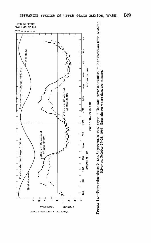
16, 1966________-_____-______-_-___-____- 2215. Chehalis River 0.5 nautical mil.! downstream
from Wishkah River on Ocxobei 27-28, 1966. 2316. Selected sites during the period November 29-
December 3, 1966___-__-____-____-____-- 24 17-21. Graphs showing:
17. Difference between velocities at 20 and 80 percent of total depth in the Chehali^ River 0.5 nautical mile downstream from the Wish kah River on October 27-28, 1966_ _ _ ____ 25
18. Relation between rate of change of tidal stage and mean velocity in the vertical at mean time________--___----_----__-_____- 27
19. Relation between rate of change of tidal stage and mean velocity in the vertical at mean time plus 30 minutes._____________________ 28
20. Longitudinal variation of harbor cross-s?ctionalarea.____________________________________ 29
21. Relation between vertical salinity-incrementratio at Cow Point and fresh-water discharge. _ 30
22-24. Graphs showing longitudinal variation of mean salinity at high- and low-water slack on:
22. Four days in April, May, and August ^"fl..... 3223. Three days in August, September, and October
1966_______________________________ 3324. Three days in October and November lf%___ 34
25-34, Graphs showing:25. Predicted longitudinal variation of mean salinity
at mean high water for various fresh-water discharges_______________________________ 35

CONTENTS V
FIGURES 25-34. Graphs showing Continued Page26. Longitudinal variation of exponents W and W
on August 19, 1966_______________ B3627. Relation between fresh-water discharge and lon
gitudinal-dispersion coefficients_____________ 3828. Longitudinal variation of the cumulative mean
age of fresh water at various discharges______ 3929. Comparison of computed and predicted values
for cumulative mean age of fresh water at various discharges_______________________ 40
30. Longitudinal variation of cumulative travel- time of fresh water, computed at various discharges. __ _____________________________ 42
31. Relation between tidal range and average dis tance of half-cycle salinity excursion_ ______ 43
32. Excursion distances of peak dye concentrationat various fresh-water discharges.___________ 44
33. Farthest excursion distances of peak dye con centration during floodtide for various dye- injection sites..___________________________ 45
34. Farthest excursion distances of peak dye con centration for various dye-injection sites dur ing ebbtide___-_____-__________-__________ 46
35-39. Graphs showing relation between excursion distance of peak dye concentration and time after high tide:
35. At Hoquiam for surface and bottom injection?under similar conditions__________________ 47
36. At Hoquiam for a surface injection.___________ 4837. At Hoquiam for a bottom injection.___________ 4938. At Hoquiam for two surface injections.________ 5039. At Cosmopolis for a surface injection._-_-___.- 51
40-47. Graphs showing relation between excursion distance of peak dye concentration and time after low tide at Hoquiam:
40. For two surface injections in the south channel0.5 mile downstream from Cow Point _____ 52
41. For a surface injection in the north channel 0.2 mile upstream from the Hoquiam River on June 3, 1966__.___._.--______-..--.._-_-- 53
42. For a bottom injection in the north channel 0.2 mile upstream from the Hoquiam River on July 19, 1966----------------------------- 54
43. For a surface injection in the north channel 0.2 mile upstream from the Hoquiam River on October 12, 1966.____---___--------_. ----- 55
44. For a surface injection in the north channel 7.3 miles upstream from the harbor entrance on October 14, 1966_ _._. __ - 56
45. For a surface injection at Cow Point on Novem ber 27, 1966-_---_--_-_-______--_-------- 57

VI CONTENTS
FIGURES 40-47. Graphs showing relation, etc.. Continued Page46. For surface injections in the mouths of the
Wishkah and Hoquiam Rivers on August 17, 1965-_-_-.___._______.__.._.___.___._.__ B58
47. For several surface injections on August 18, 1965- 59 48. Map showing cross sections and individual midchannel
sites sampled for bottom sediments.________________ 6049-53. Graphs showing:
49. Longitudinal distribution of carbon content ofbottom materials-______-____----__________ 68
50. Comparison of longitudinal variations of carbon content of channel-bottom materials and dissolved-oxygen content of harbor water. _ _ 70
51. Relation between chemical oxygen demard andcarbon content of bottom materials________ 71
52. Relation between carbon content and amount of fine sediment for main channel bottom materials _________________________________ 72
53. Relation between salinity intrusion and fresh water discharge at high tides ranging from 6.5 to 11.5 feet..___._______._-.__.__._. 75
54-55. Graphs showing fluctuations of specific conductance, dissolved oxygen, and tidal stage on July 2, 1966:
54. At the Cosmopolis monitor.._________________ 7655. At the Hoquiam monitor..___________________ 77
TABLES
Page TABLE 1. Drainage areas of streams tributary to Grays Hart or_ __ B7
2. Altitudes of tidal reference planes at Port Dock andPoint Chehalis_____--__---__---___-------__------ 12
3. Tidal separation distances computed from At/-________ 264. Particle-size analyses of the coarse fraction of Grays
Harbor bottom-material samples collected in June 1966. 615. Particle-size analyses of composited fine fractions of
Grays Harbor bottom-material samples collected in June 1966__----_---------_---____------__.___. 64
6. Carbon content of bottom-material samples, GraysHarbor_-________--___ _________- _- --_-- 64
7. Mean values and standard deviations of daily marimum and minimum automatic-water-quality-monitor data for the period May through September 1966.________ 79
8. Correlation matrix for daily maximum and minimum automatic-water-quality-monitor data for the period May through September 1966-_-__----------------- 80

ENVIRONMENTAL QUALITY
ESTUARINE STUDIES IN UPPER GRAYS HARBCR WASHINGTON
By JOSEPH P. BEVERAGE and MILTON N. SWECKER
ABSTRACT
Improved management of the water resources of Grays Harbor, Wash., requires more data on the water quality of the harbor and a better understanding of the influences of industrial and domestic wastes on the local fisheries resources. To provide a more comprehensive understanding of these influences, the U.S. Geo logical Survey joined other agencies in a cooperative study of Grays Harbor. This report summarizes the Survey's study of circulation patterns, descriDtion of water-quality conditions, and characterization of bottom material in the upper harbor.
Salt water was found to intrude at least as far as Montesano, 28.4 nautical miles from the mouth of the harbor. Longitudinal salinity distributions were used to compute dispersion (diffusivity) coefficients ranging from 842 to 3,520 square feet per second. These values were corroborated by half-tidal-cycle dye studies. The waters of the harbor were found to be well mixed after extended periods of low fresh-water flow but stratified at high flows. Salinity data were used to define the cumulative "mean age" of the harbor water, which may be used to approxi mate a mean "flushing time."
Velocity-time curves for the upper harbor are distorted from simple harmonic functions owing to channel geometry and frictional effects. Surface and bottom velocity data were used to estimate net tidal "separation" distance, neglecting vertical mixing. Net separation distances between top and bottom water ranged from 1.65 nautical miles when fresh-water inflow was 610 cubic feet per second to 13.4 miles when inflow was 15,900 cubic feet per second. The cumulative mean age from integration of the fresh-water velocity equation was about twice that ob tained from the salinity distribution.
Excursion distances obtained with dye over half-tidal cycles exceeded those estimated from longitudinal salinity distributions and those obtained by earlier investigators who used floats. Net tidal excursions were as much as twice those obtained with floats.
The carbon content of bottom materials was related to channel fine material:
C=0.315 + 0.0238 F
where C is in percent by dry weight, and F is percent by weight finer than 0.062 millimeter. Carbon content was low upstream and downstream of the uppe" harbor
Bl

B2 ENVIRONMENTAL QUALITY
area, and high in the Cow Point-Rennie Island reach. The high-carbon-content reach coincides with the general area of a dissolved-oxygen sag.
The logarithm of the fresh-water discharge gave a high degree of correlation with daily maximum specific conductance at Cosmopolis. The regression equation is:
#Cma*=76.4-l7.71ogioQ/
where Kcm** is in millimhos at 25° Celsius (centigrade), and Q/ is the estimated daily fresh-water discharge, in cubic feet per second.
Dissolved oxygen is the most critical water-quality parameter in Grays Harbor. At Cosmopolis, the daily minimum dissolved oxygen content, DOcmin, correlated well with discharge and tidal range, AJEf. The regression equation relating the vari ables is:
DOCmi n= 6.03 + 0.00096 Q/-0.291A#
in which DOcmin is in milligrams per liter and AJEf is in feet.The upper harbor was found to contain 250 million cubic feet less water than
average during the critical low-flow period, on the basis of the frequency distribu tion of predicted tides. About 78,000 pounds of dissolved oxygen if thus unavail able for oxidation of waste during summer.
INTRODUCTION
Grays Harbor is a large estuary on the Pacific coast of Washington, roughly 50 miles north of the Columbia River and about the same distance west of Olympia, the State capital. The harbor entrance is formed by two long, low sand spits (fig. 1). These spits are the western boundaries of the North and South Bays. The upper harbor, which is the area described in this report, connects the Chehalh River with the lower harbor and the North and South Bays. Most field data were collected in the area extending from Montesano on the east to the confluence of the North arid South Channels on the wept, a channel distance of about 22 nautical miles.
Wood-products industries have dominated the economic activity in the harbor area since the late 1800's. The lumber, plywood, and pulpmills use harbor waters only for log storage and effluent disposal, whereas the fish and shellfish industries require relatively unpolluted harbor waters.
Several instances of dead or distressed fish have occurred in the upper harbor in the past 40 years. Most kills have be Q,n found to coincide with extremely low dissolved oxygen, although low pH played a part in early fish kills (Eriksen and Townsend, 1940).
The present investigation developed from a common desire of private, State, and Federal groups to investigate more, thoroughly the pollution problem in Grays Harbor. The common objective of the group was to determine the basic water-quality conditions, the factors influencing the water quality, and the effects of this environ ment on the aquatic organisms.

fHum
ptu
Iips
Riv
er
Hoq
uiam
Abe
rdee
nM
onte
sano
-28.
4(0)
LOC
ATI
ON
O
F PR
OJE
CT
AREA
FIG
UR
E 1. S
ket
ch m
ap o
f G
rays
Har
bor.
Dot
s ar
e sp
aced
at
1-m
ile i
nter
vals
, st
arti
ng
at
mou
th o
f ha
rbor
. N
umbe
rs o
utsi
de p
aren
th
eses
ind
icat
e na
viga
tion
-cha
nnel
dis
tanc
es u
pstr
eam
fro
m m
outh
. N
umbe
rs i
nsid
e pa
rent
hese
s in
dica
te d
ista
nces
dow
nstr
eam
fr
om S
tate
Hig
hway
107
bri
dge
sout
h of
Mon
tesa
no.
Sha
ded
area
s in
dica
te t
idal
fla
ts.
Map
mod
ifie
d af
ter
U.S
. C
oast
and
Geo
de
tic
Sur
vey
Cha
rt 6
195,
59t
h ed
., M
arch
21,
196
6.til CO

B4 ENVIRONMENTAL QUALITY
By cooperative agreement between the U.S. Geological Survey and the Washington State Pollution Control Commission, the U.S. Geo logical Survey led the investigations of the physical and chemical water-quality conditions, estuary hydraulics, and bottom material.
The scope of the Survey's investigation was limited to describing the general circulation and water-quality conditions of the water mass and the influence of bottom materials on the water-quality conditions. The description of circulation involved determination of the movement and dispersive characteristics of the water mass by means of dye, current-meter, and salinity studies. The description of the water's quality was primarily an assessment of longitudinal salinity distributions and of the record from two automatic water- quality monitors, which recorded water temperature, specific con ductivity, and dissolved oxygen. The influence of bottom materials on water-quality conditions was to be determined indirectly by re lating carbon content of the materials to their chenrical oxygen demand.
The Pollution Control Commission led the investigations of fish migration and distribution, determined the amount and quality of industrial and domestic wastes entering the upper harbor, and de termined the relative magnitude of wastes supplied ty tributary streams.
Other agencies associated with the study, and their arers of investi gation, were the Washington State Department of Fisheries (phyto- plankton and productivity studies), the Washington State Depart ment of Game (compilation of fish migration records from prior studies), and the Weyerhaeuser Co. (respiration of bottom materials and supplemental water-quality data collection).
A composite report will be released informally by the Pollution Con trol Commission. The Geological Survey's contribution to the investi gation is reported here more formally and in greater detail than in the composite report.
ACKNOWLEDGMENTS
The U.S. Geological Survey's segment of the investigation was car ried on under the supervision of L. B. Laird, Washington district chief, Water Resources Division. The writers gratefully acknowledge the cooperation of the Pollution Control Commission (R. M. Harris, Director) and the assistance given by E. H. Olson and D. R. Fisher of the Weyerhaeuser Co., Cosmopolis.
PREVIOUS INVESTIGATIONS
Eriksen and Townsend (1940) reported on studies conducted by the Pollution Control Commission during 1938-39. They outlined the

E'STUARINE STUDIES IN UPPER GRAYS HARBOR, WASH. B5
sources of pollution and observed several instances of distressed and dead fish, shrimp, and crabs. The only pulp mill on the harbor r,t that time, owned by Rayonier, Inc., was found to contribute most of the waste effluent to the harbor, in terms of BOD (biochemical oxygen demand). Sulfite waste liquor, the principal mill pollutant, was shown to be harmful to fish in the laboratory and to cause a large depletion of available dissolved oxygen. By utilizing longitudinal chlorinity distri butions at low-river flow and upper harbor volumes, they calculated a 1.2-percent exchange of water each tide (from mean higher high water to mean lower low water) in the upper harbor. Minimum diseolved- oxygen concentrations, in percent of saturation, were then related (p. 45-46) to fresh-water discharges less than 4,000 cfs (cubic feet per second). No BOD analyses of harbor inflow were given, although an estimated BOD loading of 7,500 pounds per day was given (p. 16), based on untreated domestic sewage per capita upstream. The estimate of BOD loading contributed by the mill was 260,000 pounds per day. Bottom muds were found to have an effect on the dissolved oxygen only if the muds were disturbed and became mixed with harbor voters.
The Pollution Control Commission has investigated conditions in Grays Harbor several times since 1939. Orlob, Jones, and Peterson (1951) studied water conditions and water use relative to the effect of domestic and industrial waste effluent. More than 86 percent of the organic waste load during low-river flow was attributed to sulfite waste material. Reportedly, a dissolved-oxygen level of 5.0 mg/1 (milligrams per liter), considered critical to fish, was reached when sulfite waste liquor concentration reached 40 mg/1, and water temperature ex ceeded 18°C (Celsius). For temperatures from 14° to 18°C, the critical dissolved-oxygen level was reported to have been reached when sulfite waste liquor concentration was about 60 mg/1. To improve dissolved- oxygen conditions in the harbor, they concluded, waste-liquor recovery efficiencies would have to be improved and waste-liquor dis charge would have to be regulated according to ability of waters to assimilate those wastes. Also, the coliform concentration due to domes tic sewage wastes had exceeded the recommended Public Health Serv ice water-quality standard a maximum of 1,000 coliforms per 100 milliliters for the culture of shellfish. Restrictions were subsequently placed on the quantities of fish and shellfish that could be taken within the harbor.
Later Pollution Control Commission investigations of Grays Harbor were those by Peterson (1953) and by Peterson, Wagner, and Livingston (1957). The 1953 survey was made to determine any improvement in bacteriological quality of harbor waters, and the 1957 survey was made to determine water-quality conditions prior to

B6 ENVIRONMENTAL QUALITY
completion of the harbor's second pulp mill, which wa<* being built by the Weyerhaeuser Co. The 1957 report noted that sulfite waste liquor affects salmonids by lowering the dissolved oxygen to critical levels and by increasing toxicity. Toxic effects were not considered critical until sulfite waste liquor concentrations were so high that the lowered dissolved-oxygen level already was injurious to the salmonids. During the 1956 low-flow period, the area of low dissolved oxygen existed from Cosmopolis to the Hoquiam River. The most critical area extended from the Wishkah River to Cosmopolis, and the con ditions were worst at approximately high tide.
A thorough survey of the literature of Grays Harbor through 1954 was prepared by Bader, McLellan, and others (1955). Their report provides abstracted material for the reader and gives tl e location of unpublished material.
A model study of effluent distribution in Grays Harbor was described by Bialkowsky and Billington (1957). They found that a sevenfold reduction of the waste concentration could be expected by locating the proposed Weyerhaeuser Co. effluent outfall in the Cow Point reach, as opposed to an outfall at Cosmopolis. They found a slight advantage in limiting effluent discharge to ebbing tide.
Pearson and Holt (1960) documented several examples of low dissolved-oxygen concentrations at the harbor entrance during summer floodtides. The low concentrations were associated with low water temperatures, and thus were considered to be the result of occasional summertime upwelling of oxygen-poor oceanic water off the coast. They estimated a deficiency of 1,700 tons of oxygen (less than satura tion) in incoming water during one tidal cycle in 1956. Although not all of this deficit would occur in upper harbor waters, they pointed out the need for considering the actual dissolved oxygen of the ocean water when figuring oxygen balances in estuaries.
HYDROLOGY
This section of the report gives a general background for the more specific sections that follow. Spatial and temporal distribution of fresh-water discharge are discussed first; then tides, tidal character istics, and tidal influence are discussed.
FRESH WATER
Fresh water from four rivers passes through Grays Harbor. The Chehalis River, the largest, drains about 80 percent of the area tributary to the harbor. Tributary drainage areas are given in table 1 (Richardson, 1962). Only the Chehalis, Wishkah, and Hoiuiam Rivers drain directly into the project area. The other streams given in the table probably have only a slight effect on upper harbor hydraulic

ESTUARINE STUDIES IN UPPER GRAYS HARBOR, WASH. B7
TABLE 1. Drainage areas of streams tributary to Grays HarborDrainage
r .. area Location (sq mi)Chehalis River above Wishkah River, at Aberdeen._______________ 2, 012
Satsop River at gaging station near mouth.________________ 299Wynoochee River at U.S. Highway 410 near mouth.____ _ _ 185
Wishkah River at mouth, U.S. Highway 410 at Aberdeen.___________ 102Hoquiam River at mouth, U.S. Highway 101 at Hoquiam____________ 90. 2Humptulips River near mouth, at State Highway 9C________________ 245Johns River near mouth, at State Highway 13A_____________________ 31. 3Elk River at mouth___----------------_---_---_-_______________ 18. 2Miscellaneous tributaries_________________________________________ 51. 4
Total____________________________________________________ 2, 550. 1
and water-quality characteristics. The effects of the other streams have been ignored in this study.
The Chehalis River is not gaged below Porter. Porter is 14 miles upstream from Montesano, which is at the eastern end of the esfriary. The Satsop River joins the Chehalis about 6 miles upstream from the State Highway 107 bridge at Montesano. The Wynoochee River enters the Chehalis about 300 yards downstream from the same bridge. The annual mean discharges at Porter and at the farthest downstream gaging stations on the Wynoochee and Satsop Bivers for the periods of record are given in figure 2. The similarity of runoff response is evident.
Wynoochee River
1930 1940 1950
WATER YEAR
1960
FIGTJEE 2. Annual mean discharges of Chehalis River at Porter, Satsop River near Satsop, and Wynoochee River above Save Creek, for periods of record through water year 1965.

B8 ENVIRONMENTAL QUALITY
The monthly mean discharges for the same three stations for water year 1965 are given in figure 3. Note that all three stations record minimal flow during July, August, and September. The monthly precipitation pattern for water year 1965 is also given in figure 3 (U.S. Weather Bureau, 1966, p. 231). Surface runoff is obviously related to precipitation similarly in the three watersheds. The esti-
Oct Nov Dec Jan Feb Mar Apr May June July Aug Sept 1964 1965
FIGURE 3. Monthly mean discharges of Chehalis River at Porter, Satsop River near Satsop, and Wynoochee River above Save Creek, and monthly pre cipitation at Aberdeen, for water year 1965.

ESTUARINE STUDIES IN UPPER GRAYS HARBOR, WASH. B9
Jan Aug Sept Oct Nov Dec
FIGURE 4. Estimated daily discharge of Chehalis River at Hoquiam during calendar years 1965 and 1966.
mated composite daily discharges at Hoquiam for calendar years 1965 and 1966 are shown in figure 4. The discharges of the Chehalis River near Grand Mound (about 18 miles upstream from Porter), the Satsop River near Satsop, and the Wynoochee River below Black Creek near Montesano (about 20 miles downstream from Save Creek) were estimated from gage-height readings, usually taken once daily at 0800 P.s.t. No effort was made to adjust the values for traveltime differences, but a 40-percent increase war made to account for the increase in drainage areas of the Wishks,h and Hoquiam Rivers, which are not gaged. The discharges are thus an estimate of fresh water which flowed into the upper harbor during this study. Throughout the study these discharges were taken as the fresh-water discharge, usually as daily values but sometimes averaged

BIO ENVIRONMENTAL QUALITY
over several days. As noted above, low flow (less than 1,000 cfs) typically occurred during July, August, September, and the first part of October. This same pattern was followed in both years.
The flow-duration curves for the period of record through 1964 are given in figure 5 for the same three stations used in figures 2 and 3.
10,000
y 1000 -
1001 5 10 20 50 80 90 95 99
PERCENTAGE OF TIME GIVEN DISCHARGE WAS EQUALED OR EXCEEDED
99.9
FIGURE 5. Flow-duration curves for Chehalis River at Porter, Satsop River near Satsop, and Wynoochee River above Save Creek, for period of record through water year 1964.
Although the curves have not been combined into a composite graph, the similar shapes and slopes of the curves add further corroboration for similarity of watershed response to precipitation. Moreover, the similarity of shape allows use of the Satsop curve with 36 years of record for estimating low-flow frequency of the entire basin. For the concurrent period of annual mean flow used in figure 2, 1953-65, the Satsop River flow was 29.1 percent of total mean flow. The Satsop River discharges were obtained from figure 5 for frequencies of 99.7, 86.3, 72.6, 67.1, 61.6, and 58.9 percent (corresponding to 1, 10, 50, 100, 120, 140, and 150 days per year, respectively). The^e discharges were then converted to an equivalent composite Chehalis River

ESTUARINE STUDIES IN UPPER GRAYS HARBOR, WASH. Bll
discharge by dividing by 0.291. The resulting values are plotted in figure 6. This curve is the trend for the period of record only, however,
3000
2500 -
2000 -
1500 -
I 1000 -
AVERAGE NUMBER OF DAYS EACH YEAR DISCHARGE LESS THAN INDICATED MEASUREMENT
FIGURE 6. Estimated flow-duration curve for Chehalis River at Hoquiam for period 1930-65.
322-777 O «9 3

B12 ENVIRONMENTAL QUALITY
and projection of the curve to future periods should be made with caution. From the curve, fresh-water flow less than 1,000 cfs occurred 43 days per year, on the average.
TIDES
The tides along the Washington coast are of the mixed type a higher and lower high tide each lunar day as well as a higher and lower low tide. The mean and diurnal tidal ranges are 6.9 and 9.0 feet, respectively, at the harbor entrance at Point Chehalis (U.S. Coast and Geodetic Survey, 1965). These same values increase to 7.8 and 9.9 feet at Aberdeen, and then decrease to 6.7 and 8.1 fe°it at Mon- tesano. Tidal terms used in this report are as follows: MTL (mean tide level), MHW (mean high water), MHHW (mean higher high water), MLW (mean low water), and MLLW (mean lower low water). The mean range is defined as the difference in stage between MHW and MLW, and the diurnal range is defined as the difference between MHHW and MLLW. MLLW is the standard datum for the U.S. Coast and Geodetic Survey Chart 6195, and for figure 1.
Altitudes of various tidal planes for Point Chehalis and Port Dock are given in table 2. Port Dock values were used as reference planes
TABLE 2. Altitudes, in feet above mean lower low water, of tidal reference planes at Port Dock and Point Chehalis, Grays Harbor
[Data from U.S. Coast and Geodetic Survey, 1958, 1965]
Tidal plane Port Dock Point C'lehalis
Highest tide.. _______ _____MHHW __MHW. ____________________Mean tide level _MLW ____ . ___ . ___ _MLLW. ___________________Lowest tide- _ _____________
__________ 15.29. 90
____________ 9.20____________ 5.30_________ _ 1. 40
. 00_-___-__--._ -2.9
14. 0±0. 59. 008. 304. ?51.40
. 00-3. 0±0. 5
for this study throughout the upper harbor. During the summer months, however, these reference planes are not accurate. This is shown in figure 7 which gives cumulative-frequency curves computed from 1966 predicted tides at Port Dock (U.S. Coast and Geodetic Survey, 1965, p. 90-93). Median high- and low-tide stages for the full year are about half a foot higher than similar values for the 3-month low fresh-water flow period, July-September. The median values (equaled or exceeded by 50 percent of the tides) are 9.3 and 8.9 feet for high tide, and 1.6 and 1.1 feet for low tide, respectively.
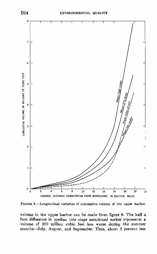
A plot of cumulative volume of the upper harbor with distance downstream from Montesano is given in figure 8. Tidal reference planes (MHW, MTL, and MLW) used in this figure are approximately

ESTUARINE STUDIES IN UPPER GRAYS HARBOR, WASH. B13
14
12
High tides
04-
2 -
0 -
Low tides
-210 20 50 80 90 95 99
PERCENTAGE OF TIDES EQUALING OR EXCEEDING GIVEN STAGE
99.9
FIGURE 7. Cumulative-frequency curves for predicted tides at Port Dock, 1966. Solid and dashed lines indicate relations for entire year and for July through September, respectively.
those for Port Dock. The mean tidal prism, more accurately the intertidal volume, is simply the difference between MHW volume and MLW volume, rather than the measured volume entering the harbor on a mean floodtide (Ippen and Harleman, 1961, p. 46). The volumes in figure 8 were computed by Pollution Control Com mission personnel from a joint-agency hydrographic survey of the upper harbor made in February and March 1966. The steepness of the curves downstream from mile 14 reflect the shallow tideflat geometry typical of the harbor. As tidal waters move in and out of Grays Harbor, large expanses of tidal flats are exposed and re-covered. Eriksen and Townsend (1940, p. 29) estimated the water-surface area to be between 40 square miles at MLLW and 99 square miles at MHW. The intermediate 59 square miles of tidal flats plays an im portant role in the movement, mixing, and reaeration of harbor waters as tides ebb and flood. Much of this area is between 1 and 2 feet above MLLW. An order-of-magnitude estimate for the total
B14 ENVIRONMENTAL QUALITY
7 -
6
5 -
4 -
3 -
2 -
24 6 8 10 12 14 16 18 20
CHANNEL DISTANCE DOWNSTREAM FROM MONTESANO, IN NAUTICA'. MILES
22
FIGURE 8. Longitudinal variation of cumulative volume of the upper harbor.
volume in the upper harbor can be made from figure 9. The half a foot difference in median tide stage mentioned earlier represents a volume of 250 million cubic feet less water during the summer months July, August, and September. Thus, about 3 percent less

ESTUARINE STUDIES IN UPPER GRAYS HARBOR, WASH. B15
12
11
10
-2
-3
T I
Mean higher high water
Mean high water
Mean tide level
EXPLANATIONTidal planes
- Tidal reference plane
_. _ Calendar year 1966
July-September 1966
2345678
HARBOR VOLUME, IN BILLIONS OF CUBIC FEET
10
FIGURE 9. Relation between volume of upper harbor and tidal stage at Port Dock. Volumes were computed for reach between 8 and 28.4 miles above the mouth (fig. 1).
water would be available for dilution at MHW, and 7 percent less at MLW.
B16 ENVIRONMENTAL QUALITY
The tidal wave moves slowly up the estuary. The high-tide stage requires 29 minutes to reach Aberdeen from the harbor entrance, and another 1 hour and 24 minutes to reach Montesano (U.S. Coast and Geodetic Survey, 1965, p. 173). The passage of low tide is similar but slower.
The upstream boundary of an estuarine investigation is usually defined by the objectives of that investigation. In sediment-transport studies, for instance, the upstream boundary is the farthest upstream point that the tides influence streamflow, causing backwater. For some studies, the upstream limit of flow reversal is a more critical factor; the limit of flow reversal on the Chehalis River is several miles up stream from Montesano over most of the range of discharge. In this study, the limit of tidal influence is defined as the point of the farthest upstream intrusion of salt water; most investigators use this limit to define an estuary.
In estuarine pollution studies, the pollutants are usually expected to mix and disperse with salt water in the same manner as the fresh water mixes with the salt water. The farthest salt-water intrusion into the Chehalis is only a short distance upstream from the Montesano highway bridge at low flow. For fresh-water discharges greater than 50,000 cfs, this salt-water intrusion extends only to Cosmopolis.
The hydrology of Grays Harbor, then, is largely influenced by fresh-water inflow and by the tides. Runoff from the Chehalis River basin constitutes the major inflow of fresh water, especially to the upper harbor. During the period of this study, the 3-month low-flow period coincided with a 3-month low-tidal-stage period; thus, the volume available for dilution of municipal and industrial wastes was reduced.
HYDRAULICS OF THE ESTUARY
The rate of removal of pollutants from an estuary depends mainly upon the degree of mixing taking place within the harbor, the degra dation rate of the pollutants, the proportion of the harbor volume renewed each tidal cycle, and the net seaward velocity of the fresh water. In some instances, deposition and chemical precipitation are also important processes for removal of pollutants. The rate of pol lutant degradation is determined by the nature of the pollutant and the estuary environment. The degree of mixing depends on the loca tion of the effluent outfall, estuary geometry (large-scale circulation patterns), and the hydraulic characteristics of the estuary. In this section of the report, velocity and salinity data collected during this investigation are presented and dye studies are summarized. Also, several theoretical and empirical expressions that predict longitudinal salinity distributions are evaluated.

ESTUARINE STUDIES IN UPPER GRAYS HARBOR, WASH. B17
VELOCITY
The velocity of water in a well-mixed estuary at any given time depends on harbor geometry, tidal amplitude, fresh-water discharge, and the influence of bottom sediments. Velocity is usually considered to be a harmonic function of time which is modified by frictional effects. Fresh-water discharge increases ebb currents and reduces flood currents. The time lag between high tide and high slack water (zero surface velocity) decreases with increasing discharge. The low-tide lag increases with increasing discharge.
Velocity data were obtained over several 13- to 14-hour periods and one 25-hour period in 1966. All data were obtained from a boat moored at the edge of the navigation channel. Velocities were meas ured with a Price current meter at six points in the vertical: at either 0.5 or 1.0 foot from the surface; at 0.2, 0.4, 0.6, and 0.8 of the depth (Z>); and either 1.0 or 1.5 feet from the bottom. Vertical traverses usually were made 4-10 minutes apart for most of the period. The mean velocity was computed for each vertical series by averaging the velocities at 0.2, 0.4, 0.6, and 0.8 of the depth. Mean velocities are shown in figures 10-13, along with a tidal-stage curve drawn from the predicted values (U.S. Coast and Geodetic Survey, 1965, p. 90-93).
Within the upper harbor, maximum mean velocities in the vertical vary from about 3 fps (feet per second) on floodtides to about 4.5 fps on ebbtides. The magnitude of these velocities is dependent on tidal stage, range of tides, fresh-water discharge, and location within the estuary.
The mean-velocity curves are distorted from a simple hrrmonic function. Similar distortion has been noted on the Delaware River (Miller, 1962, p. 5, 11-12) and on the Waccasassa River (Ftelzen- mueller, 1965, p. 35). Although these authors make no comment on the distortion, the truncation of the cosine curve is most likely attrib utable to channel geometry and frictional effects. The occurrence of the maximum velocity shortly after the change of tide is evidently a characteristic of upper Grays Harbor velocity-time curves.
The 0.2 velocity (velocity at 20 percent of total depth, or 0.2Z>) is representative of the motion of the upper layer of water, and, like wise, the 0.8 velocity is representative of the motion of the bottom layer. Individual measurements of the 0.2 and 0.8 velocities for a range of fresh-water discharge are plotted against time in figures 14-16. Near low tide in most of the examples, the bottom water reverses first, followed after an interval by the reversal of the upper water. Near high tide the opposite is true. On flooding ticSs, 0.2 velocities are sometimes larger, sometimes smaller, and oftec about the same as 0.8 velocities. On ebbing tides, the 0.2 velocities are always greater.

B18 ENVIRONMENTAL QUALITY
00600
_ Tidal stage
00700
Tidal stage-
MAY 18, 1966
North channel 0.2 mile ups*ream _ from Hoquiam River
Cow PointA South channel about one mile
downstream from Cow Point
Fresh-water discharge 3000 cfs
0700 0800 0900 1000 1100 1200 1300 1400 1500 1600 170C 1800 1900
MAY 19, 1966
I I I
North channel 0.5 mile downs'ream from Hoquiam River
North channel 0.2 mile upstreamfrom Hoquiam River
A Hoquiam River 02 mile upstreamfrom mouth
Fresh-water discharge 2600 cfs
____ I I I I I0800 0900 1000 1100 1200 1300 1400 1500 1600 1700 1800
PACIFIC STANDARD TIME
1900 2000
FIOUBE 10. Mean velocities and predicted tidal stages at selected sites during the period May 18-19, 1966.
The differential movement between upper and lower layers deter mines the mixing of pollutants. The data upon which f ̂ ures 14-16 are based allow computation of a net separation after t, tidal cycle. Figure 17 is a typical plot of time and AE7, the difference between the 0.2 velocity and the 0.8 velocity. Each of the previous observation periods was similarly computed and plotted. The curves ^ere planim- etered by tidal period, and the areas under the curves were converted to "separation distances." The separation distance concent naturally has no true validity but is of some use when considering large-scale mixing of pollutants. The separation distance is the interval separating surface and bottom waters after a tidal cycle of movement in the harbor when a frictionless horizontal sheet has been placed at mid-

ESTUARINE STUDIES IN UPPER GRAYS HARBOR, WASH. B19
4
s 3S 2ts. L
I 1
-1
! -2I
1 -3
-4
_ "Tidal stage
I I I I Fresh-water discharge: 670 cfs
' -'Velocity
North channel 0.5 nautical mile downstream from Hoquiam River, Sept. 14, 1966
1000 1200 1400 1800 2000 2100
Fresh-water discharge: 590 cfs
% -Velocity
%
I I I I
Chehalis River 0.5 nautical mile upstream from Elliott Slough, Sept. 15, 1966
I I I I I I I I0900 1300 1500 1700 1900
- Fresh-waterdischarge: 570 cfs
**. Tidal stage
-Velocity
Chehalis River 0.5 nautical mile downstream from Wishkah River, Sept. 16, 1966
I I1400 1600 1800
PACIFIC STANDARD TIME
2200 2300
FIGURE 11. Mean velocities and predicted tidal stages at selected sites duringthe period September 14-16, 1966.
322-777 O 6i9 i

gCD
i
0
cT 2.
ot> <rt- P
CfQQ DO O v o" 0
s £
to a oo
pCn
B
I
S2 > *oE3
MEAN VELOCITY, IN FEET PER SECOND
UPSTREAM DOWNSTREAM
I I r-o H o i co
I I I I
o i~o ^ o> oo t; i O (NO
PREDICTED TIDAL STAGE, IN FEET

ESTUARINE STUDIES IN UPPER GRAYS HARBOR, WASH. B21
1 I I l I i I
_ Fresh-water discharge: 14,800 cfs/--~ Tidal stage
-3 0
5
4
3
2
1
0
-1
-2
-3
^-VelocitySouth channel 3.5 nautical
miles downstream from Cow - Point, Nov. 29, 1966I I I I I I I
1500 1700 1900
Fresh-water discharge: 19,500 cfs
Velocity- -Tidal stage
North channel 0.5 nautical mile downstream from Hoquiam River, Nov. 30, 1966
08004
2200 2310n i i i i i i rFresh-water discharge: 9510 cfs
^^
-Tidal stage Velocity-
I I
Chehalis River 0.5 nautical mile downstream from Wishkah River,Dec.1-2, 1966
I I I I I I I I1500 1700 1900 2100 2300
I I I TFresh-water discharge
35,600 cfs
J__L
Chehalis River 0.8 nautical mile upstream from Elhott Slough, Dec. 2-3, 1966
I I I I I I I I I1600 1800 2000 2200
PACIFIC STANDARD TIME
FIGURE 13. Mean velocities and predicted tidal stages at selected sites during the period November 29-December 3, 1966.

B22 ENVIRONMENTAL QUALITY
= -i >-
- ^/Velocity at 20 percent of total depth
elocity at 80 percent of total depth
North channel 0.5 nautical mile downstream from Hoquiam River, Sept. 14, 1966
4
3
2
1
0-1
-2
~3
-4
1 I I I I I Fresh-water discharge_
670 cfs
1400 1600 18001 1 1 I I I I
Fresh-water discharge 590 cfs
Velocity at 20 percent of total depth
_ Velocity at 80 percent of total depth
I I I I
Chehalis River 0.5 nauticalmile upstream from Elliott -
. Slough, Sept. 15, 1966
1400 1600 1800 * 2000
10 8 6 4 2 0
-2
6 4 2 0
-2
2200 2300 12
Fresh-water discharge 10 570 cfs
Velocity at 20 percent of total depth
Velocity at 80 percent// of total depth
I I I I I
,'xCnehalis River 0.5 nautical mile downstream from
I Wishkah River, Sept. 16,, 1966
0800 1200 1400 1600 1800
PACIFIC STANDARD TIME
2000 2200 2300
FIGURE 14. Point velocities at 20 and 80 percent of total depth at selected sites during the period September 14-16, 1966. Long dashes indicate missing data.
VELOCITY, IN FEET PER SECOND
UPSTREAM DOWNSTREAM
I I I
M 3
Iso o
^ s- Cfi CD S "g. CD g:
CDr^-^ o 2 s*^ B*tr g.
S. < ST CD p i-j
S5 P a> Cn
g. JTa o
III Mlo r*o -^ o^ oo ^ Irt
PREDICTED TIDAL STAGE, IN FEET

B24 ENVIRONMENTAL QUALITY
n I I r
South channel 3.5 nautical miles downstream from Cow Point, Nov. 29, 1966
I I I I I I I I I I I I
II I I
I I I I I I
North channel 0.5 nautical mile downstream from Hoquiam River, Nov. 30, 1966
I I I I I 1 I I1000 1200 1600 1800 2000
i i r
Chehalis River 0.5 nautical mile downstream from Wishkah River, Dec. 1, 1966
I I"1200 1408 1608 1800 2000 2200 2400"
Velocity at 20 pen r- of total depth
^Velocity at 80 percent\ / of total depth \ '______ Vw
I I I I
' VChehalis River 0.8 nauticar^ mile upstream from Elliott
, Slough, Dec. 2-3, 1966 . ,
1000 1200 1400 1600 1800 2000 2200 2400 0200
PACIFIC STANDARD TIME
FIGURE 16. Point velocities at 20 and 80 percent o* total depth at selected sites during the period Novem ber 29-December 3, 1966. Gaps shown where datr, are missing.

VELOCITY DIFFERENCE (At/), IN FEET PER SECOND
UPSTREAM DOWNSTREAMI
J_______I I I I 'I IO K> J^ CD 00 I *-
O N>
PREDICTED TIDAL STAGE, IN FEET

B26 ENVIRONMENTAL QUALITY
depth. The net separation distances, given in table 3, generally decrease as the fresh-water discharges decrease.
TABLE 3. Tidal separation distances computed from AU
Date (1966)
Sept.
Oct.
Nov.
Dec.
14....
15....
16
27.....
28
29
30....
1
2
3-day average
Site fresh-water discharge
(cfs)
0.5 mile downstream from mouth of Hoquiam River.
0.6 mile downstream from mouth of Wishkah River.
.do .
..do.
0.5 mile downstream from mouth of Hoquiam River.
0.6 mile downstream from mouth of Wishkah River.
700
670
610
6,400
5,000
13,000
15,900
25,900
32,900
Tide
Flood. Ebb-Net. ..Flood.....Ebb .Net. ..Flood.....Ebb......NetEbb.......Flood.....Net.......Ebb.......
NetFlood.....Ebb .Net.. .Flood. .Ebb .TMfttFlood.. Ebb.......Net...... .Flood. Ebb...... .Net. .
Tidal cycle (hr)
... 6.75 5.50... 12.25 .... 7.00... 5.75... 12.75 .... 6.50... 5.47... 11.97 .... 6.25... 6.50... 12.75 .... 8.15
.85... 9.00 .... 6.00... 6.50... 12.50 .... 5.67... 7.50... 13.17 .... 4.25... 8... 12.25 .... 4.2... 9.1... 13.3 .
Separation Tidal distance range (nautical
(ft) miles)
8.5 9.5
11.7 10.9
11.5 11.7
9.2 8.2
7.2 8.4
6.9 11.7
6.6 11.6
6.1 11.0
5.6 10.2
-0.96 3.72 2.76
-.96 4.32 3.36
-2.05 3.70 1.65 4.40 .17
4.57 4.83 .51
5.34 -1.82
5.30 3.48 4.76 8.67
13.4 2.94 3.62 6.56 .36
3.28 3.64
The mean velocity in the vertical was related to the time rate of change of tidal stage for one 26-hour period, on October 27-28, 1966 (fig. 18). The relation was improved somewhat by usin^ the mean velocity for half an hour after the mean time of the tidal difference, as shown in figure 19. None of the other velocity runs were as simply related.
The net movement of estuarine waters over a long t'mespan, as postulated by the quasi-steady-state model, can be inferred from the fresh-water velocity. The mean fresh-water velocity at any cross section is dependent on the cross-sectional area, which varSs through out the estuary. Cross-sectional areas obtained during the 1966 U.S. Geological Survey-Pollution Control Commission hydrogrs t>hic survey are shown in figure 20 for MTL and MLW. The exponential equation representing the line for MTL is:
Ax = (1)
where AXjn is cross-sectional area in square feet, and xm is channel dis tance in, nautical miles downstream from Montesano. For MLW, the equation is:
..wo, (2)

ESTUARINE STUDIES IN UPPER GRAYS HARBOR, WASH. B27
3
1 2 3
MEAN VELOCITY AT MEAN TIME (f), IN FEET PER SECOND
FIGURE 18. Relation between rate of change of tidal stage ( AH/ AO and mean velocity in the vertical at mean time (?) 0.5 nautical mile down stream from the Wishkah River on October 27-28, 1966.
where Ax is cross-sectional area and x is channel distance from the mouth. The reference point for each equation was chosen to be suitable for a particular use. For both equations, channel distance was taken longitudinally through the tidal flats separating the north and south channels. Distance between the mouth and State Highway 107 bridge south of Montesano is considered to be 27.6 nautical miles, rather than 28.4 miles, because cross-sectional area include? both north and south channels, when straight-line distance through the large tidal flat separating the two channels is used. Channel distances, therefore, do not quite agree with those in figure 1. By definition:
Qf=Ax Ux , (3)
where Qf is the fresh-water discharge; Ax is the cross-sectional ?.rea at x, the longitudinal distance from an origin; and Ux is the mean cross-
322-777 O ©9 5

B28 ENVIRONMENTAL QUALITY
o Ebb tide
Flood tide
0123
MEAN VELOCITY AT 7 + 30 MINUTES, IN FEET PER SECOND
FIGURE 19. Relation between rate of change of tidal stage (A/// A<) and mean velocity in the vertical at mean time (f) plus 30 minutes 0.5 nautical mile downstream from the Wishkah River on October 27-28, 1966.
sectional velocity at x due to fresh-water discharge. Therefore, mean fresh-water velocity is given by equations 1 and 3:
AXm 3,700e-0.200im . (4)
This equation will be used in the next section to derive the age of fresh water moving through the estuary.
SALINITY DISTRIBUTION
Salinity is the term given to dissolved salts in estuarine and oceanic waters and is usually reported as parts per thousand. These salts are transported into an estuary by a combination of diffusion, large-scale circulation, and differential transport. Diffusion is the phj'sical process by which solutes tend toward uniform concentration. Large-scale circulation is a matter of harbor geometry, tides, and fresh-water dis-

ESTUARINE STUDIES IN UPPER GRAYS HARBOR, WASH. B29
1,000,000
CHANNEL DISTANCE DOWNSTREAM FROM MONTESANO, IN NAUTICAL MILES
26 24 22 20 18 16 14 12 10 8 64 2
100,000 -
10,000
30004 6 8 10 12 14 16 18 20 22 24
CHANNEL DISTANCE UPSTREAM FROM MOUTH, IN NAUTICAL MILES
26 28
FIGURE 20. Longitudinal variation of harbor cross-sectional area. Open circles mean low water; solid circles mean tide level.
charge. Differential transport refers to the net separation distance discussed earlier, whereby the upper, less salty layer moves a greater net distance during a tidal cycle than does the lower layer. Vertical diffusion and turbulence tend to equalize the vertical salinity gradient. Increased fresh-water discharge accentuates the differential transport due to the pumping action of the tides and reduces vertical mixir'?:.
Grays Harbor is reasonably well mixed vertically during low-flow periods lasting several weeks or more. Figure 21 indicates the effect of fresh-water discharge on the ratio of the top-to-bottom salinity dif ference to the mean vertical salinity, As/ s, at Cow Point for 1966 data.

B30i.o
ENVIRONMENTAL QUALITY
0.8 -
0.7 -
0.6
0.5 -
0.4
|= 0.3 -
0.2
0.1
0.0
o High-water slack
Low-water slack
123456789 10
FRESH-WATER DISCHARGE, IN THOUSANDS OF CUBIC FEET PER SECOND
FIGUKE 21. Relation between vertical salinity-increment ratio (As/ s) at Cow Point and fresh-water discharge. Off-scale ratio (3.36) at 10,400 cfs (low-water slack) is not shown.
Despite the scatter of points, the trend toward increasing: As/ s with in creasing discharge is apparent. Conversely, small salinity gradients occur at low discharges.
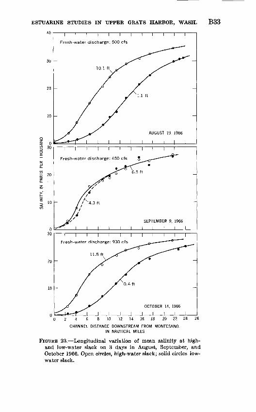
Longitudinal distributions of mean salinity obtaired in Grays Harbor during 1966 are given in figures 22-24. These plcts are slightly distorted because of practical difficulties in obtaining adequate definition of the distribution while keeping pace with the tidal wave. Usually, salinity runs were begun in the lower harbor about 20 minutes before tide change and completed at the upper end an hour or two after tide change.
Ketchum (195la, b) modified the classical tidal-prism method of estimating estuarine flushing. His works gave early insight into flushing processes and stimulated much of the interest in the general study of estuaries since 1950. Ketchum's predicted salinity distribu tions (fig. 25) place much greater quantities of salt in the upper

ESTUARINE STUDIES IN UPPER GRAYS HARBOR, WASH. B31
reaches than has been observed (figs, 22-24) . Evidently, the inter^idal volume of each segment does not mix completely with its concomitant basal volume at high tide as assumed in Ketchum's method. Further comparisons are made below under the discussion of mean age.,
Many mathematical models of longitudinal salinity distribution (Stommel, 1953; O'Connor, 1961; Ippen and Harleman, 1961) are based on the assumption of seaward movement due to the fresh-water velocity (the quasi-steady-state model). Calculations show that net movement at low flow during one tidal cycle (eq 4) is much smaller than the "net separation distance" given in table 3. For mathematical simplicity, most models are designed for an artificial estuary which is well mixed vertically and has a constant cross-sectional area. Investi gators in the field must then determine the degree of similarity be tween the conditions in the definition model and actual conditions in the estuaries which they are studying.
Ippen and Harleman (1961) derived a theoretical model for longi tudinal salinity distribution at low tide in a long rectangular fume with constant mean fresh-water velocity. For the quasi-steady state, they found:
-=e-W(x+B)2 > (5) s0
where s is the mean salinity in the vertical, s0 is the salinity of the nearby ocean, x is the channel distance upstream from the mouth, B is the distance seaward from the mouth to the region of constant salinity, and where.
in which D'0 is the apparent eddy diffusivity at the estuary entrance. W, Ux, B, and S0 are considered to be constant.
For Grays Harbor, B seems to range from 0 to about 5 nautical miles depending on the littoral current (Budinger and others, 1964, p. 52) and fresh- water discharge. During most of the summer low-flow period, B was small. Taking the logarithms of both sides of equation 5,
(7) and
The variation of W with channel distance (eq 8) for the Augus4: 19, 1966, salinity data are given in figure 26. W can be considered constant for only a short distance from mile 6 to mile 14 and then it in creases almost linearly with channel distance. The dashed line W is

B32 ENVIRONMENTAL QUALITY
30
20
10
20
10
I 0 < 40
30
20
10
\ \ \\ \ \ \ \\ \
Fresh-water discharge: 8,000 cfs
10.2 ft
APRIL 5-6, 1966
i r i T 7
Fresh-water discharge: 2,000 cfs
\ \ \ \ \ \ \ \ \ \
Fresh-water discharge: 630 cfs
AUGUST 2, 1966
\l\\024 6 8 10 12 14 16 18 20 22 24 26
CHANNEL DISTANCE DOWNSTREAM FROM MONTESANO, IN NAUTICAL MILES
FIGURE 22. Longitudinal variation of mean salinity at high- and low-water slack on 4 days in April, May, and August 1966. Open circles, high-water slack; solid circles, low-wate~ slack.
ESTUARDSTE STUDIES IN UPPER GRAYS HARBOR, WASH. B33
40
30 -
20 -
10
< 0a 30 o
20
3 10
20
10
I I I I I I
Fresh-water discharge: 500 cfs
I I I I I
i i i i \ i i r
Fresh-water discharge: 450 cfs
J__L
SEPTEMBER 9, 1966
I I I I III
i I I I I I I T T
Fresh-water discharge: 930 cfs
10 12 14 16 18 20 22 24 260246
CHANNEL DISTANCE DOWNSTREAM FROM MONTESANO, IN NAUTICAL MILES
FIGUBE 23. Longitudinal variation of mean salinity at high- and low-water slack on 3 days in August, September, and October 1966. Open circles, high-water slack; solid circles low- water slack.

B34 ENVIRONMENTAL QUALITY
30
20
10
30
20
10
20 -
10 -
i i i r I i iFresh-water discharge: 7,500 cfs
I I I I I I I I
Fresh-water discharge: 2,150 cfs
I I I \ \ 1I
Fresh-water discharge: 10,300 cfs
11.0ft
i r
0.2 ft
NOVEMBER 26, 1966
I I I I I I0 2 4 6 8 10 12 14 16 18 20 22 24 26
CHANNEL DISTANCE DOWNSTREAM FROM MONTESANO, IN NAUTICAL MILES
FIGURE 24. Longitudinal variation of mean salinity at high- and low-water slack on 3 days in October and November 1966. Open circles, high-water slack; solid circles, low-water slack.

ESTUARINE STUDIES IN UPPER GRAYS HARBOR, WASH. B35
40
2 30
10 -
2 4 6 8 10 12 14 16 18 20 22 24
CHANNEL DISTANCE DOWNSTREAM FROM MONTESANO, IN NAUTICAL MILES
26
FIGURE 25. Predicted longitudinal variation of mean salinity at mean high water for various fresh-water discharges, on the basis of Ketchum's method (1951a).
a plot of W, where B Q, divided by channel distance. Where B is not equal to zero, similar relations would be obtained. The part of the curve for which W is approximately constant, upstream of mile 11 (airport), is the region of greatest interest in this study, but W is no longer dimensionally correct. Whether the dependence of W on x in this part of the curve is because of variations of U, or D0', or both (eq 6) is not known.
For W to be constant in a natural estuary, the term In s/s0 must be proportional to (x-\-B) 2 . Salinity data taken on^August 19, 1966, seem to indicate that in upper Grays Harbor, In s/s0 is mor^- nearly proportional to x3 . However, the mean velocity varies exponentially with x (eq 4), not directly, as W would imply.
For constant mean fresh-water velocity throughout the region of an estuary, O'Connor (1961, pp. 564-565) obtained a similar equation for the quasi-steady state:
-Ux
s=sne (9)
where s is the mean salinity at x, s 0 is the oceanic salinity, and e is322-777 O '69 6

B36 ENVIRONMENTAL QUALITY
0.007
CHANNEL DISTANCE DOWNSTREAM FROM MONTESANO, IN NAUTICAL MILES
20 10 0
0.006
0.005
0.004
0.003
0.002
0.001
10 20
CHANNEL DISTANCE UPSTREAM FROM MOUTH, IN NAUTICAL MILES
30
FIGURE 26. Longitudinal variation of exponents TF(from eq. 8; solid lines) and W (dashed line) on August 19, 1966. Numbers indicate assumed values for the variable B in equation 8.

ESTUARINE STUDIES IN UPPER GRAYS HARBOR, WASH. B37
the turbulent transport coefficient. 1 If mean fresh-water velocity varies in the longitudinal direction, as it does in Grays Harbor, O'Connor suggested comparison of an e computed from equation 9, assuming a longitudinally averaged mean velocity, with an e computed from the finite-difference equation:
where 2Ax is the length of an estuary segment with linearly varying salinity, sx is the mean salinity over the segment, U is the mean velocity through the segment, and the denominator is the salinity difference between downstream and upstream boundaries of the segment. The mean velocity was computed for the midpoint of the segment at MLW from equations 2 and 3 :
Q/" 160*, (U)
where x is measured in nautical miles upstream from the mouth.The relation between fresh-water discharge and the longitudinal
average e computed from equation 10 is given in figure 27. The diffusivities were computed directly from low- tide field data following extended periods of reasonably constant flow, with 2 Ax taken as the distance between sampling stations. High-tide cUffusivity value*' were somewhat larger, and diffusivities computed from the slopes of semi- logarithmic plots of salinity and channel distance were much greater than those computed from the finite-difference equation. The line in figure 27 represents the power equation derived from a logarithmic plot of the upper three diffusivities computed from equation 10. This equation is not strictly correct because the dispersion coefficient is not zero at zero fresh-water discharge (J. D. Stoner, written corrmun., 1967). Diffusion would continue to take place owing to tidal action as long as a salinity gradient existed. O'Connor (1961, p. 607) showed a logarithmic plot of e with Qf and obtained a reasonably constant relation. He also noted (p. 604) the leveling off of diffusivity with increasing discharge.
Longitudinal salinity distributions are of some help to the estnarine hydrographer in estimating the "flushing rate" of harbors. Ketchum (1951a, p. 202-203) presented a method of estimating the mean age of harbor waters from his predicted longitudinal salinity. In figure 28,
i In this report no effort has been made to separate diffusion from dispersion. Although eacl author's label has been followed, the turbulent-transport coefficient above is considered equivalent to the apparent- diffusion coefficient and dye-dispersion coefficient discussed later. This is because of the equations used which lump all effects into a single coefficient. Hereafter, these terms are used interchangeably, except when a distinction as to computational method is desired.

B38 ENVIRONMENTAL QUALITY
< o
= 300 0
o e , eddy-diffusivity coefficient
Dx, dye-dispersion coefficient
a 0 1 2 3 4 5 6 7 8 9 10 11 12 13 14
m FRESH-WATER DISCHARGE, IN THOUSANDS OF CUBIC FEET PER SECOND
FIGURE 27. Relation between fresh-water discharge and longitudinal-dispersioncoefficients.
this method has been reversed. The mean age of fresh water was computed from high-water-slack field data for 2-nautical-mile seg ments. Mean age is taken as the number of tidal cycles at constant discharge required to replace the fresh-water fraction of the MHW segment volume. Although a single salinity distribution would not be necessarily representative of equilibrium condition^, mean age computed from an average distribution should be representative. Figure 28 also shows a cumulative mean-age curve that was computed from the average of 1965 weekly low-flow (less than 80C cfs) salinity runs by the Weyerhaeuser Co. (D. R. Fisher, Weyerhaeuser Co., written commun., 1966). The average tidal stage for the Y^eyerhaeuser salinity runs is more than a foot lower than that for curves computed from individual runs. The expected trend with fresh-water discharge is shown in the figure cumulative mean age decreases rapidly with increasing Qf.
A qualitative "mean flushing time" may be estimated f-om figure 28 by taking the differences in mean ages between the point of pollutant injection and a given point downstream. Also, for a known degrada tion rate of the pollutant it should be possible to estimate which reach would be most affected by the pollutant.

ESTUARINE STUDIES IN UPPER GRAYS HARBOR, WASH. B39
fr 40 -
ii
30 -
20 -
10 -
-2 0 2 4 6 8 10 12 14 16 18
CHANNEL DISTANCE DOWNSTREAM FROM MONTESANO, IN NAUTICAL MILES
FIGURE 28. Longitudinal variation of the cumulative mean age of fresl water at various discharges, based on salinity data for high-water slack. Curve for 600 cfs represents an average of data from weekly low-flow salinity runs during 1965 (D. R. Fisher, Weyerhaeuser Co., written commun., 1966); other curves are based on single runs.
Ketchum (1951a, p. 204) compared data from Raritan estuary with predicted values and found good agreement throughout much of the the estuary. In figure 29, cumulative mean-age data from Grays Harbor are plotted against cumulative mean age from Ketchum's computation for 2-nautical-mile segments downstream from Monte-

B40 ENVIRONMENTAL QUALITY
sano. There is an apparent trend toward equality between computed and predicted mean ages at higher discharges. However, this trend is probably due more to the rapid movement of fresh water out of the upper harbor at high discharge than to the more complete mixing postulated in Ketchum's method. At the lower end of the curves, there is little difference between the 1,000-cfs and 8,000-cfs relations.
20
<-> 15
10
EXPLANATIONFresh-water discharge, in
cubic feet per second
o 500
1000
A 2000
A 8000
10 20 30 40
COMPUTED CUMULATIVE MEAN AGE, IN TIDAL CYCLES
50 60
FIGURE 29. Comparison of computed and predicted values for cuirulative mean age of fresh water at various discharges. Computed values are from field data collected at high-water slack; predicted values are based on Ketchum's method (1951a).
Another way of thinking of "mean age" is in terms of time of travel. Traveltime can be obtained from the equation for fresh-water velocity by integrating equation 4:
TT ^ V* p-0.20Qxm.Ux -dt 3,700 e (12)
Separating variables,
dt =3,700 Q,- 1 e°- 200x dx, (13)

ESTUARESTE STUDIES IN UPPER GRAYS HARBOR, WASH. B41
integrating, and evaluating (at t =0, xm=ty,
*(sec)=112.5X10⁶ Qf-^e0 -*00* 1), (14)
and converting to time in tidal cycles,
£=2,520 Qj-V200*"-!). (15)
Equation 15 for several discharges is shown in figure 30. The cumu lative mean age from longitudinal salinity distributions (fig. 28) is about half of the fresh-water traveltime for a given location. O c course, equation 15 is based on longitudinal variation of cross-sectional area at MTL, whereas the computations for figure 28 were based on high- water-slack data. Had equation 15 been based on MHW, which would have been incorrect for the steady-state condition, the frerh-water traveltime would have been still larger. On the other hand, had the mean-age curves been based on longitudinal salinity distribution at MTL, the use of Ketchum's method would cast serious doubt on the curves, because of his definition of exchange ratio intertidal volume divided by high-tide volume.
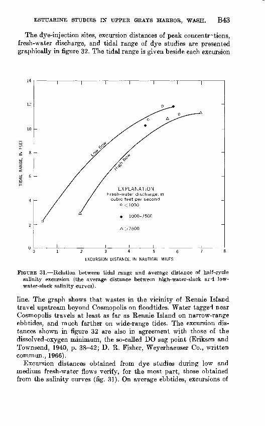
Finally, longitudinal salinity distributions are of use in estimating tidal excursion distances. The average distance between the high- and low-tidal curves in figures 22-24 can be taken as the estimated half- tidal-cycle distance. These excursion values will be somewhat shorter than true values, however, because the water is not really "tagged" with salts as it would be with dye. Between any two consecutive slack tides, dilution of saline water with fresh water produce? a mix ture which blurs the reidentification of a given portion of harbcr water. The point of maximum dye concentration is assumed always to be the small volume of water into which the dye was injected. F'gure 31 relates tidal range to the average excursion distance. Excursion dis tance is seen to increase as both tidal range and discharge increase.
DYE STUDIES
The movement of the water in the upper part of Grays Harbor was traced with fluorescent dye (rhodamine B) placed in the water by a slug-injection technique. The excursion of the dye cloud wae defined by continuously sampling with fluorometers from boats. Both longi tudinal and vertical definitions of the dye clouds were obtained by sampling while the boat moved slowly through the dye cloud and then anchoring the boat and sampling as the cloud moved past, and by sampling at different depths at various locations along the river channel. The method of sampling depended upon whether the dye was injected at the surface or near the bottom. The dye was

B42
150
ENVIRONMENTAL QUALITY
140 -
130 -
120
110
100
90
80
70
60
50
40
30
20
10
2 4 6 8 10 12 14 16 18 20
CHANNEL DISTANCE DOWNSTREAM FROM MONTESANO, IN NAUTICAL MILES
22
FIGURE 30. Longitudinal variation of cumulative traveltime of fresh water, computed at various discharges from equation 15.
tracked for only half a tidal cycle, on an ebbing or flooding tide, because of restrictions on dye quantities allowed per dump. Dye concentrations dropped to background readings after 5-8 hours. Interfering substances included sulfite waste liquor and phytoplank- ton. The low and variable fluorescence of sulfite waste liquor precluded tracking it in the harbor.
ESTUARINE STUDIES IN UPPER GRAYS HARBOR, WASH. B43
The dye-injection sites, excursion distances of peak concentrations, fresh-water discharge, and tidal range of dye studies are presented graphically in figure 32. The tidal range is given beside each excursion
14
10
EXPLANATION Fresh-water discharge, in
cubic feet per second o <1000
1000-7500
A >7500
01234 5678
EXCURSION DISTANCE, IN NAUTICAL MILES
FIGURE 31. Relation between tidal range and average distance of half-cycle salinity excursion (the average distance between high-water-slack ard low- water-slack salinity curves).
line. The graph shows that wastes in the vicinity of Rennie Island travel upstream beyond Cosmopolis on floodtides. Water tagged near Cosmopolis travels at least as far as Rennie Island on narrow-range ebbtides, and much farther on wide-range tides. The excursion dis tances shown in figure 32 are also in agreement with those of the dissolved-oxygen minimum, the so-called DO sag point (Eriksen and Townsend, 1940, p. 38-42; D. R. Fisher, Weyerhaeuser Co., written commun., 1966).
Excursion distances obtained from dye studies during low and medium fresh-water flows verify, for the most part, those obtained from the salinity curves (fig. 31). On average ebbtides, excursions of

B44
25
ENVIRONMENTAL QUALITY
Q 20
15
10 11.1 <-11.2
11.5
10.9 <-7.4
11.8 <H
12.5
13.413.0
5 10 15
CHANNEL DISTANCE DOWNSTREAM FROM MONTESANO, IN NAUTICAL MILES
20
FIGURE 32. Excursion distances of peak dye concentration at various fresh water discharges. Circle indicates dye-injection site, and arrowhead indicates direction and farthest extent of excursion. Tidal range is shown ?,t arrowhead.
7.7-8.6 nautical miles were obtained, whereas excursions- of 5.7-8.8 miles were obtained on average floodtides. Net tidal excursion, then, was as much as 2.0 miles seaward during the dye studies. F-riksen and Townsend (1940, p. 35) gave tidal excursion distances obtained with floats. The floats traveled from 7.46 to 8.44 miles on ebbtides and from 6.32 to 7.85 miles on floodtides. The average net flor,t-excursion distance was 0.66 miles seaward per tidal cycle.

ESTUARINE STUDIES IN UPPER GRAYS HARBOR, WASH. B45
The four major factors affecting excursion distance are the direction of flow, amount of fresh-water discharge, tidal range, location of dye- injection site, and estuary geometry. Dye-excursion distances are plotted with the locations of the dye-injection sites in figure 33 for floodtides, and in figure 34 for ebbtides. For floodtides, the largest excursions are associated with low discharge and wide tidal range. The dye seems to travel farther when introduced in the lower part of the estuary on floodtides than when it is introduced upstream. For ebbtides, the largest excursions are associated with high discharge and wide tidal range, as well as with upstream injection locationr
Individual excursion distance-time relations are presented in figures 35-47.
The movement of bottom water was traced with dye several times for conditions of discharge and tidal range similar to those of the surface
10
3 -
2 -
1 -
7.4
+ 7.4
°12.6
Sb11 - 8°=Lll.l
31 if 5 jjlO.9
11.0
68.3 Xll.3
O
6.7A
8.9
K:4 08.3
,7-4 ®8.3
8.9
EXPLANATIONFresh-water discharge, in cubic feet per second
o<1000
<1000; bottom injection
A 1000-10,000
A > 10,000
0 5 10 15 20
DYE-INJECTION SITE, IN NAUTICAL MILES DOWNSTREAM FROM MONTESANO
FIGURE 33. Farthest excursion distances of peak dye concentrator during floodtide for various dye-injection sites. Symbol "X" within circle indicates dye injection in main river channel, with resulting excursion up tributaries. Symbol "-)-" indicates dye dump at mouth of tributary. Tidal range is given beside each symbol. Dye injection was at surface unless otherwise irdicated.

B46
10
9
8
co 7LU '
^
IN NAUTICAL l\CT>
uj 5z
CO
Q
z 4 oEXCURSI
CO
2
1
n
ENVIRONMENTAL QUALITY
A 12.1
_
1
A 12 ' 5
.13.0
| 0 13.4
cM
- op
X
1_ 0.
I
0 O
~
1 13
o4.8
EXPLANATIONFresh-water discharge, in
cubic feet per second
o <1000
<1000; bottom injection
A 1000-10,000
A > 10,000
+ South channe injections
1 1
1
^
J13.6
13.6
ennie Island
-
o 4 - 2
'c
+
"
3.6 3.6
15 10 15
DYE-INJECTION SITE, IN NAUTICAL MILES DOWNSTREAM FROM MONTES4NO
FIGURE 34. Farthest excursion distances of peak dye concentration for various dye-injection sites during ebbtide. Tidal range is given beside each symbol. Dye injection was at surface unless otherwise indicated.
runs. The bottom ebbtide excursion in figure 35 (dashed curve) is shorter than the surface excursion under similar conditions namely, low flow and narrow range of tides. For low flow and a wide tide range, dye introduced at the bottom of the north channe1 (fig. 37) traveled within a third of a mile of the distance traveled by surface- released dye (fig. 38). The length of time to travel the distance, how ever, was about 45 minutes longer for the bottom-released dye than for the surface-released dyt. On the only bottom floodtide release (fig. 42), the dye traveled farther than the similar surface trace (fig.
ESTTJARINE STUDIES IN TIPPER GRAYS HARBOR, WASH. B47
10
Fresh-water discharge 745 cfs
765 cfs
Tidal range 3.6 ft
3.65 ft
3 -
300 400
TIME AFTER HIGH TIDE, IN MINUTES
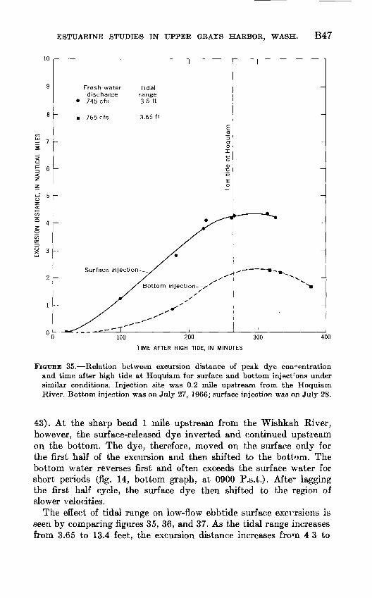
FIGURE 35. Relation between excursion distance of peak dye concentration and time after high tide at Hoquiam for surface and bottom inject'ons under similar conditions. Injection site was 0.2 mile upstream from the Hoquiam River. Bottom injection was on July 27, 1966; surface injection was on July 28.
43). At the sharp bend 1 mile upstream from the Wishkah River, however, the surface-released dye inverted and continued upstream on the bottom. The dye, therefore, moved on the surface only for the first half of the excursion and then shifted to the bottom. The bottom water reverses first and often exceeds the surface water for short periods (fig. 14, bottom graph, at 0900 P.s.t.). Afte~ lagging the first half cycle, the surface dye then shifted to the region of slower velocities.
The effect of tidal range on low-flow ebbtide surface exci^rsions is seen by comparing figures 35, 36, and 37. As the tidal range increases from 3.65 to 13.4 feet, the excursion distance increases from 4 3 to

B48
10
ENVIRONMENTAL QUALITY
Fresh-water discharge: 790 cfs Tidal range: 4.2 ft
100 200
TIME AFTER HIGH TIDE, IN MINUTES
300 400
FIGURE 36. Relation between excursion distance of peak dye concentration and time after high tide at Hoquiam for a surface injection. Dye vas injected in the north channel at the mouth of the Hoquiam River on Jul;- 29, 1966.
8.1 nautical miles. The increase of excursion due to an increase in discharge is seen by comparing figures 38 and 39.
Figure 40 allows the comparison of two floodtide dye traces origi nating in the south channel near Cow Point. Doubling the discharge decreased the excursion distance about 20 percent.
A comparison of figures 41 and 43 would seem to contradict earlier statements regarding the effect of discharge on floodtide surface ex cursions. However, $ye movement in these tests was more complex. Peak dye concentrations on June 3, 1966 (fig. 41), were found at 11- foot depth after they had traveled only 2.5-3 miles, and near the bottom ab@ut 1.5 miles upstream from the Wishkah Eiver. On October 12, 1966, however, the peak concentrations were found

ESTUARINE STUDIES IN UPPER GRAYS HARBOR, WASH. B49
10
9 -
7 -
6 -
5 -
3 -
2 -
Fresh-water discharge: 560 cfs Tidal range: 13.6 ft
ioa 200TIME AFTER HIGH TIDE, IN MINUTES
300 400
FIGURE 37. Relation between excursion distance of peak dye concentration and time after high tide at Hoquiam for a bottom injection. Dye was injected in the north channel 0.2 mile upstream from the Hoquiam River on August 16, 1966.
similarly on the bottom about a mile upstream from the T^ishkah River, but the dye had shifted much later. Whether or not these shifts in depth were caused by density effects is not known.
By comparing figure 44 with the October 13 curve in figure 40, the effect of estuary geometry becomes apparent. Advancing up the estuary, water from the western part of the estuary does not en counter as much of the force of the fresh-water discharge as water in the eastern part of the estuary. This increased force due to fresh water no doubt accounts for the 12-percent reduction in the excursion of upstream water.
Figure 45 shows the only dye trace that lasted much more than half a tidal cycle. Some appreciation of water movement is gained by observing the trace. Following a 5.5-mile upstream excursion on the

B50
10
ENVIRONMENTAL QUALITY
Fresh-water discharge: 560 cfs Tidal range: 13.4 ft
T
-S x I100 200 300
TIME AFTER HIGH TIDE, IN MINUTES
400
FIGURE 38. Relation between excursion distance of peak dye concentration and time after high tide at Hoquiam for two surface injections. Dye was in jected in the north channel 0.2 mile upstream from the Hoquiam River (solid line and dots) and in the Chehalis River at Cosmopolis (dashed line and squares) on August 17, 1966.
floodtide, the tagged water traveled possibly 10 miles downstream. The different excursion distances for floodtides and ebbtides are due to the effects of discharge and difference in tidal ranges.
Finally, figures 46 and 47 compare tributary and upstream excursion- time relations during floodtides. The flatter slopes of these curves clearly show the slower velocities and shorter excursion distances in the tributaries. The nearly identical relations for the Hoiuiam and Wishkah Rivers (fig. 46) reflect similar effects of discharge and tides. The Peels Slough curve (fig. 47) illustrates the much slowe'1 velocities and excursion distances in sloughs.

ESTUARINE STUDIES IN UPPER GRAYS HARBOR, WASH. B51
Fresh-water discharge: 13,500 cfs Tidal range: 13.4 ft
200 300
TIME AFTER HIGH TIDE, IN MINUTES
400
FIGURE 39. Relation between excursion distance of peak dye concentration and time after high tide at Cosmopolis for a surface injection. Dye was in jected in the Chehalis River at Higgins Island on November 28, 1966.
Dye-dispersion coefficients were computed from the one-dimen sional diffusion equation, using values of the variance for different times computed by the method of moments:
(16)Sc
in which c is the dye concentration, in parts per billion, and x is the longitudinal distance, in feet, from a reference point, such as the con centration peak. The dispersion coefficient, Dx , was taken as one-half the slope of a line drawn by eye through a plot of <rx2 against the time after the dye dump (Diachishin, 1963a, p. 37). However, the line was

B52
10
ENVIRONMENTAL QUALITY
~ 4
Fresh-water discharge
820 cfs
1690 cfs
Tidal range 11.5ft
10.8 ft
100 200 300
TIME AFTER LOW TIDE, IN MINUTES
400
FIGURE 40. Relation between excursion distance of peak dye concentration and time after low tide at Hoquiam for two surface injections in the south channel 0.5 mile downstream from Cow Point. Circles represent Octo ber 13, 1966, injection; dots represent June 2 injection.
not forced through the origin; only the computed points wer«, used to determine the line. Three values computed in this manner from ebb tide dye data are shown in figure 27. The figure shows reasonable agreement between dye-dispersion coefficients and those from LWS (low-water slack) salinity data using equation 10. The agreement is surprising, considering that Dx represents dispersion over only half a tidal cycle. The e values represent dispersion over mr.ny tidal cycles and are probably an approximation of equilibrium conditions. The dye studies usually were limited to half a cycle because of the relatively small amounts of dye that were used. Also, the dye did not always disperse throughout the cross section. The dye cloud had a tendency to remain stratified especially during the higher fresh water discharges. This would indicate only partial vertical mixing during a half-tidal cycle.
When a contaminant is added to an estuary, the rate of dissipation (flushing) of the contaminant depends on the proportion of the harbor

ESTUARINE STUDIES IN UPPER GRAYS HARBOR, WASH. B53
10
^ 5
Fresh-water discharge: 1770 cfs Tidal range: 11.0 ft
0 100 200 300 400
TIME AFTER LOW TIDE, IN MINUTES
FIGURE 41. Relation between excursion distance of peak dye concentration and time after low tide at Hoquiam for a surface injection in the nortl channel 0.2 mile upstream from the Hoquiam River on June 3, 1966.
volume replaced each tidal cycle (by saJt and fresh water) and the dispersion rate. The dispersion coefficient describes the rate of expan sion of the contaminated volume and the rate of decrease of the contaminant concentration. The data contained in this report provide a basis for estimation of the movement (excursion and circulation patterns) of a contaminated water mass and, if the appropriate degradation constants are known, the estimation of approximate concentrations of industrial or municipal pollutants.
SUMMARY OF ESTUARY HYDRAULICS
Maximum mean tidal velocities approach 3 fps (feet per second) upstream and 4.5 fps downstream, depending on tides (extremes and range), location, and fresh-water inflow. These velocities are far greater than those due to fresh-water discharge computed from equation 4. A comparison of velocities for 0.2 and 0.8 of depth shows

ENVIRONMENTAL QUALITY
Fresh-water discharge: 980 cfs Tidal range: 11.1 ft
200 300
TIME AFTER LOW TIDE, IN MINUTES
400
FIGURE 42. Relation between excursion distance of peak dye concentration and time after low tide at Hoquiam for a bottom injection in the north channel 0.2 mile upstream from the Hoquiam River on July 19, 1966.
that water at the surface (0.2 velocities) moves faster, on the average, than water at the bottom (0.8 velocities). The hypothetical separation distance between surface and bottom waters after a tidal cycle varied from 1.65 to 13.4 nautical miles. An attempt to relate mean velocity directly to the rate of change of tidal stage was satisfactory in only one instance.
Longitudinal-salinity data were used to estimate eddy diffusivities and tidal excursion distances, and to evaluate the long'tudinal- salinity-distribution models of Ketchum (1951a), Ippen and Harleman (1961), and O'Connor (1961). The simplest theoretical model, that of O'Connor, was assummed correct in regard to diffusivity coefficients because the values used appeared to be more reasonable. Diffusivity coefficients computed from equation 10 were related to fresh-water discharge. The coefficients ranged from 842 to 3,520 square feet per second, and discharge ranged from 500 to 8,000 cfs. Although Ketch-

ESTUARINE STUDIES IN UPPER GRAYS HARBOR, WASH. B55
Fresh-water discharge: 740 cfs Tidal range: 10.9 ft
= 7
6 -
5 -
100 200 300 400
TIME AFTER LOW TIDE, IN MINUTES
FIGURE 43. Relation between excursion distance of peak dye corcentration and time after low tide at Hoquiam for a surface injection in the north channel 0.2 mile upstream from the Hoquiam River on October 12, 1966.
urn's method did not describe the field data, his approach was used to estimate the mean age of fresh water from field data. Mean age computed in this manner was then compared with mean age computed from Ketchum's model.
Dye studies were made to follow the movement of water in the upper harbor and to obtain dispersion coefficients for comparison with those calculated from salinity data. The excursion distances obtained from dye studies were greater than those obtained from float studies (Eriksen and Townsend, 1940) and those estimated from high- and low-slack salinity distributions. For average tides, the excursion distance averages about 8 nautical miles during ebb anc1 7 miles during flood. Net excursion during a tidal cycle was as much as 2 miles during the dye studies.
Dye-dispersion coefficients corroborated those computed from salinity distributions. Considering the field problems in determining

B56 ENVIRONMENTAL QUALITY
10
^ 7
uj- 5
^ 4
Fresh-water discharge: 930 cfs Tidal range: 12.6 ft
100 200
TIME AFTER LOW TIDE, IN MINUTES
300 400
FIGURE 44. Relation between excursion distance of peak dye concentra tion and time after low tide at Hoquiam for a surface injection in the north channel 7.3 miles upstream from the harbor entrance on Octo ber 14, 1966.
dye distribution, the salinity-dispersion coefficients are considered more valid than dye-dispersion coefficients, especially for calculations involving long-term dispersion. This is because dye-dispersion coeffi cients were obtained from data collected only during half a tidal cycle.
Dispersion coefficients are necessary for calculations of pollutant- dispersion patterns, assimilative capacities, and predicted concentra tion values. The literature contains papers by several authors who make use of diffusivity or dispersion values (O'Connor, 1961, 1965; Diachishin, 1963b; Camp, 1965; and Waldichuk, 1966). Dispersion values given by these authors support those obtained in Grays Harbor. Furthermore, values and relations given in this report could be used with some of the approaches described by these other investigators to estimate the assimilative capacity or the pollutant- distribution pattern of the harbor. However, such an estimate is beyond the scope of this report.

ESTUARINE STUDIES IN UPPER GRAYS HARBOR, WASF!. B57
Fresh-water discharge: 10,800 cfs Tidal ranges: 6.7 ft (floodtide) and
11.1 ft (ebbtide)
200 300 400 500
TIME AFTER LOW TIDE, IN MINUTES
600
FIGURE 45. Relation between excursion distance of peak dye concentration and time after low tide at Hoquiam for a surface injection at Cow Point on November 27, 1966.
BOTTOM MATERIALS
Estuarine sediments are deposited in response to three major influences: velocity, salinity, and water temperature. Periodic back water from tides tends to cause deposition of heavier fluvial sediments in upstream reaches by greatly reducing, halting, and slowly reversing the current. Farther seaward in the estuary, lighter sediments and organic matter are deposited when tidal currents become slack, especially on neap (narrow range) tides (Gilbert, 1917, p. 25). Non- cohesive sediments might be resuspended when tidal flow has reversed direction and generated sufficient turbulence. Salinity and temperature determine the density and viscosity of the fluid, throughcnt which the sediments and organic matter are suspended; the greater the salinity and the colder the water, the less is the settling velocity of the detritus. Salinity, however, also tends to encourage flo°,culation of colloidal clays, and thereby to cause an increase in the effective size of the particle and its fall velocity. Sediments deposited within the lower reaches of a harbor are often carried back up the harbor by flood currents. This is attributable to the predominance of the bottom flood current at the mouth over the bottom ebb current. The bottom flood current is often supplied with sediment by the littoral drift (Gross and Nelson, 1966). A more complete description of estuarine sedimentation was given by Schultz and Simmors (1957).

B58
10
ENVIRONMENTAL QUALITY
i= 6
- 5
5 4
Fresh-water discharge: 735 cfs Tidal range: 8.9 ft
o Wishkah River
A Hoquiam River
D East Fork of Hoquiam River
100 200 300
TIME AFTER LOW TIDE, IN MINUTES
FIGURE 46. Relation between excursion distance of peak dye concentration and time after low tide at Hoquiam for surface injections in the mouths of the Wishkah and Hoquiam Rivers on August 17, 1965.
Dredging of harbor sediments normally is not considered as a factor influencing water quality. However, Keighton (1966, p. 11), pointed out that dredging the navigation channel interferes with the dilution or flushing process by increasing the low-tide volume, r,nd by de creasing the intertidal prism if the dredge spoils are used to fill the intertidal marshes.
SAMPLE COLLECTION
To define the possible influences of Grays Harbor bottom materials on the overlying waters, surface samples of the bottom deposits were obtained at 31 cross sections, 30 of which are shown in figure 48. Cross section 31, which is not shown in the figure, was at mile 3, near the harbor entrance (fig. 1). Samples also were obtained from the

10
ESTUARINE STUDIES IN UPPER GRAYS HARBOR, WASH. B59
^ 7
Q 4
Fresh-water discharge: 690 cfs Tidal range: 7.4 ft
Main channel (injection 0.3 mile upstream from Hoquiam River)-
Chehalis River (upstream from Peels Slough)
100 200 300
TIME AFTER LOW TIDE, IN MINUTES
400
FIGURE 47. Relation between excursion distance of peak dye concentration and time after low tide at Hoquiam for several surface injections on August 18, 1965.
first 1% miles of the Wishkah and Hoquiam Rivers (samplir? sites W1-W6 and H1-H7, respectively). Most cross sections were sampled at five equidistant points with a U.S. BM-54 bed-material sampler (Federal Inter-Agency Committee on Water Resources, Subcommittee on Sedimentation, 1958, 1963). Bottom samples were collected during April and December 1965, and March, June, and September 1966.
PARTICLE SIZE AND COMPOSITION
Particle-size determinations were made on the cross-section simples collected in June 1966 by means of sieve and visual-accumulation tube (Federal Inter-Agency Committee on Water Resources1 , Sub committee on Sedimentation, 1957). The results of the determinations are listed in table 4.

B60 ENVIRONMENTAL QUALITY
a *3 T3 «-§
9.3 . 02
^ ri
@ ga 2
-2o
-O
1 *
ISM 0
T3 ®03 tc
ft 11 ' oj T3 CQ
oj' rH
Oi 03
£ S
.00 « 03 rH O
H "d ^g S-ao

ESTUARINE STUDIES IN UPPER GRAYS HARBOR, WASH. B61
TABLE 4. Particle-size analyses of the coarse fraction (greater than 0.062 mm) of Grays Harbor bottom-material samples collected in June 1966
[The fraction greater than 1.00 mm was sieved, and that from 0.062 to 1.00mm was analyzed by the visual- accumulation-tube method. The "A" station is near the right bank (facing downstream), and the "E" station is near the left bank]
Cross section
1
2
3
4
5
6
7
8
9
10
11
Sta tion
A B C D E
A BC D E
A B C DE
A B C DE
A B C D E
A B C D E
A B C DE
A B C DE
A B C D E
A B C D E
AB C D E
Percent, by weight, finer than indicated size, in millimeters
0.062 0.088 0.125 0.175
63 3 2 94 83
2 2 2 8 72
67 3 2 29 36
30 24 80 2 93
92 7 1
12 24
39 23 1
78
636
28 3347
98 96 807 76
26
22 62 23
90 1
27 12 57
81 36 2
76 81
75 3 2 %85
3 2 28 82
82 3 2
32 48
39 25 82 5 98
95 7 1
13 26
3 10 23 1
81
75 6
28 36 49
99 98 847 78
28
22 66 26
96 2
35 13 62
88 40 2
78 83
87 8 2 98 89
10 3 2 9
91
92 4 2
50 82
56 27 85 11 100 ..
98 8 1
1729
4 10 24 1
82
86 6
29 40 52
99 99 91 8 82
32
24 70 29
98 6 44 16 69
9347 2
82 84
95 20 3 99 93
47 9 2 10 97
98 4 3 80 97
70 3288 19
99 10 9
23 33
4 12 26 1
84
95 8
33 59 60
99 10096 10 90
37
3077 40
99 20 54 24 76
96 66 4
8987
0.250
99 61 7
100 ..%
94 64 2 12 99
98 4
14 99 100 ..
80 69 92 28
100 ..35 68 31 36
4 1430 11 88
99 10 40 86 64
100
98 29 97
61
52 83 79
100 ..75 72 3389
98 93 19 95 93
0.350 0.500
100 -95 24
98
100 ..% 4 14 100 ..
99 10 87
100...
89 % 93 33
78 93 46 39
5 16 43 4394
100 ..23 53 96 68
99 61 100
81
6386 94
97 81 3797
10098 29 97 07
99 41
99
100 -19 14
99 6099
97 99 94 47
86 98 72 42
5 17 61 79 98
44 78 97 82
100 .79
93
67 87 97
99 84 39 99
99 32 97 98
1.00
100 .60
100 .
63 16
100 .90 100 .
99 100 .95 50
88 100. .88 43
6 19 73 93 100 .
6389 98 92
93
98 72 68 87 99
100 .85 41 100 .
99 35 97 99
2.00
82
95 22
100 .
100 .
95 64
91
96 46
7 21 85 100 .
76 95 98 92
99
99 78 73 88
100 .
86 44
41 98 100 .
4.00
96
100 .40
9584
100 .
100 .59
9 28 96
89 99 100 .100 .
100
100 -100 .87 94
88 51
54 100 .
8.00 16.0
100 ......
64 100
95 100 10C ......
82 100
20 100 3P 100 100 ......
100 ......100 ......
100 ...... 100 --.._.
100 _..... 66 100
8' 100

B62 ENVIRONMENTAL QUALITY
TABLE 4. Particle-size analyses of the coarse fraction (greater than 0.062 mm) of Grays Harbor bottom-material samples collected in June 1966 Continued
Cross section
12
13
14
15
16
17
18
19
20
21
22
23
24
Sta tion
A B C D E
A B C D E
A B C D E
A B C D E
A B C D E
A B C D E
A BC D E
A B C D E
A B CDE
A B C D E
A B C D E
A B C D E
A B C D E
Percent, by weight, finer than indicated size, in millimeters
0.062
92 2 73 10 83
98 72 74 31 65
96 82 12 52 75
70 97 3
21 83
92 8 2
62 92
66 65 67 51 98
88 86 30 76 97
84 65 31 54 79
19 4 3
67 73
88 48 3 97 13
9082 70 24 84
16 10 51 577
1 0 2 1 3
0.088
96 2
78 10 94
100 73 80 31 70
99 85 12 5682
81 99 3
24 92
95 9 2 70 97
75 71 71 60 99
94 91 35 85 99
94 80 37 58 83
28 4 3
70 82
96 52 3 98 19
96 88 77 25 90
18 11 56 66 8
1 0 2 1 3
0.125
99 2 89 11 98
74 84 33 75
100 88 14 62 90
94 100
5 3497
97 14 2
85 99
85 80 83 69 100
97 96 46 94 99
98 9158 67 92
44 7 3
75 89
99 66 3
98 46
98 95 91 28 96
4424 64 88 21
19 6 6 6 8
0.175
100 5
98 21 100 .
84 94 46 81
91 29 79 94
100
11 80 99
99 25 6
95 100
92 89 94 78
98 98 54 99 100
99 96 79 87 98
56 18 9
84 92
100 83 10 99 70
100 99 99 44 99
84 71 82 98 69
82 72 65 6
64
0.250
56 100 70
96 100 86 91
93 80 87 96
51 97 100
100 51 40 98
96 95 99 84
100 99 64 100
99 99 94 95 100
72 31 22 92 95
94 3499 85
100 100 76 99
97 95 94 100 92
98 98 95 68 98
0.350
90
95
99
97 98
96 99 91 98
88 100 .
82 80 100 .
99 98 100 . 90
100 93
100 100 100 98
90 56 34 97 98
99 76 100 94
92 100
99 99 99
99
100 100 99 95 99
0.500
96
98
100 .
100 .100 .
99 99 92 99
95
96 94
100 99
96
99
99
99 76 64 99 100
100 92
99
97
100 99 100
100
100 99
100 .
1.00 2.00 4.00 8.00 16.0
99 100 ............. .......
99 100 ....................
100 ...........................100 ...........................92 93 93 100 ......100 ...........................
99 100 ....................
100 ...........................98 100 --.-.-.-...-.....-.-
100 ...........................
100 ...........................
100 ...........................
100 ...........................
100 . .__-..._- ._-..-- -100 ...........................100 ......... ..................100 ...........................
100 _--.__.--.-....-..-----..
100 .----..........-..-........
100 ...........................
100 ..--.-...---. --.-
100 .-....---.... .- ----

ESTUARINE STUDIES IN UPPER GRAYS HARBOR, WASH. B63
TABLE 4. Particle-size analyses of the coarse fraction (greater than 0.062 mm) of Grays Harbor bottom-material samples collected in June 1966 Continue'!
Cross section
25
26
27
28
29
30
31
Wl W2 W3 W4 W5 W6
H3 H4 H5 H6 H7
Slipl
Slip 2
Sta tion
A BC D E
A BC D E
A BC D E
A B C DE
A BC DE
A B C DE F
A BC D E
C C C C Ccc c c c cA BC DE
AB C D E
Percent,
0.062
35 5 17 9
99
51 1
54 4 90
79 4 '0
1 26
88 1
97 82 64
62 49 99 86 39
15 45 25 86 29 60
0 0 1 0 0
21 12 3
35 65 92
20 16 58 6578
99 99 98 98 98
100 ..99 94 98 98
0.088
50 5
17 10
100
57 1
58 4 94
81 4 0 2
26
92 1
98 88 67
75 61 100 .97 45
29 56 29 93 56 75
0 0 1 0 0
22 13 3
3672 97
21 16 67 66 85
100 .100 ..100 ..100 .100 ..
100 ..99100 ..99
0.125
87 24 21 11
76 1
59 5 97
83 4 0 4
28
94 1
98 95 69
9392
100 .59
87 88 61 98 90 95
14 1 2 2 0
23 14 3
3777 98
24 18 78 67 89
99
100 .
by weight, finer than indicated size, in millimeters
0.175
99 87 41 50
93 7
62 10 99
88 8 0 10 32
96 2 99 97 71
98 99
88
99 98 92 100 .99 100 .
81 9 16 52 4
27 17 22 41 85 98
27 21 88 69 92
100 _
0.250
100 9978 91
99 64 93 55 100
95 62 27 38 42
99 53 99 98 73
99 100 .
98
100 .100 .99
100 .
98 41 65 95 31
75 46 93 54 93 99
30 28 96 72
0.350
10094 98
100 96 99 86
99 93 88 79 55
100 94 100 99 74
100 .
100 .
100 .
100 -74 89
100 -75
94 72 99 74 94 100 .
32 47 98 75 99
0.500
97 100
99 10097
100 .98 99 97 68
98
9977
83 94
92
99 80 100 .86 96
3459 99 77 100 .
1.00
99
100
100
100 .100 .100 .76
99
10078
88 95
96
99 80
88 100 .
35 59
100 .77
2.00 4.00 8.00 16.0
100 .......... ..........
87 93 100 ------
99 100 . --.
79 83 89 100
93 97 100 ......96 100 .............
98 100 .............
100 .--. . . . 90 94 100 ......
97 97 98 100
39 45 61 100 90 100 ........-.
83 85 100 ......
Material less than 0.062 mm was composited by reach and analyzed by the pipette method. These determinations are given in tr.ble 5.

B64 ENVIRONMENTAL QUALITY
TABLE 5. Particle-size analyses of composited fine fractions (finer than 0.06& mm) of Grays Harbor bottom-material samples collected in June 1966
[Approximately equal aliquots from all samples at each cross section were composited roughly by areas ofsimilar characteristics]
Percent finer than indicated siz 1?, Composite of sections in millimeters
0.002 0.004 0.008 0.016 0.031
l-4_____.__. ______5-8.. .. _..__-.. _.9-13______________14-18___---_-____-19-22____ ________25-28___-_________29-30__-____-____-W1-W6.__________H1-H7____________Slips 1, 2__________
._ __. 10_______ 4_______ 9_______ 11-_---__ 8_______ 6__--._- 8_______ 5-_---__ 8_______ 25
14412151091061031
19716191411148
1342
28102427191720101860
39133238?72534142681
The composition of the estuarine bottom materials charges radically from Montesano to the harbor entrance, a distance of 28.4 nautical miles. Near Montesano, the bottom consists of gravel with some sand; between Higgins Island (fig. 1) and the Standard Oil Co. dock (river miles 24 to 18, respectively, from the harbor entrance), the bottom is predominantly sand. From the Standard Oil dock through the Cow Point reach (mile 15), the bottom is clay with some sand; downstream to the harbor mouth, the bottom is mostly sand. Channel-side deposits in the Chehalis River upstream from the confluence of the Wishkah River are predominantly clay with some sand and organic material. There, coarse material is deposited within the channel. In the harbor area, from Cow Point to the entrance, bottom materials consist uniformly of sludge beds across the channel. Dredging operations however, tend to remove these sludge beds from the navigation chan nel; this leaves a fairly clean sand for part of the cross section and sludge over the remainder that part undisturbed by dredging.
The total carbon content of each sample was determined by using an induction-furnace carbon analyzer. The values are given in table 6.
TABLE 6. Carbon content of bottom-material samples, Grays Harbor
Channel Cross distance sec- from tion mouth
(nautical miles)»
1 21.8
Carbon content (percent by weight)
Section description
150 yd downstream from light 8, above Cosmopolis.
Sta tion 2
A B C D E
1965
Apr. Nov.
1.60 ........16 ........21 ........03 .......
1.09 .......
Dec.
1.51 .28 .03 .07
2.26
Mar.
1.14 .16 .09 .03
3.71
1966
June
1.58 .27 .56
1.72 r\47
Sept.
1.66 .18 .30 .19
5.55
Avg.
1.498 .210 .238 .408
4.616See footnotes at end of table.

ESTUARINE STUDIES IN UPPER GRAYS HARBOR, WASH. B65
TABLE 6. Carbon content of bottom-material samples, Grays Harbor Continued
Channel
sec- from
(nauticalmiles)»
2 21.7
3 19.8
4 19.6
5 18.2
6 18.0
7 17.2
8 16.9
9 15.8
10 15. 6
11 15. 5
12 15. 4
13 15. 3
Carbon content (percent by weight)
Section description
300 yd downstream fromlight 8.
Under powerline atCosmopolis.
At Cosmopolis monitorsite, light 5.
At navigation light atmouth of Elliott Slough.
200 yd downstream fromStandard Oil Co. dock.
At light 1, mouth ofWishkah River.
At Anderson-Middletonincinerator, 300 yddownstream fromTJPRR bridge belowWishkah River.
Cow Point reach, southfrom light 59.
Cow Point reach, northfrom double rangemarker.
Cow Point reach, betweencross sections 10 and 12.
Cow Point reach, northfrom light 20.
Cow Point reach, southfrom light 57.
Sta-
ABCDE
ABCDE
ABCDE
ABCDE
ABCDE
ABCDE
ABCDE
ABCDE
ABCDE
ABCDE
ABCDE
ABCDE
Apr.
2.14 .1.14.14.09 .
10.4 .
1.37 ..17 ..15 ..29 .
1.03 .
4.33 ..18 ..33.20 .
1.66 .
2.93 .1.80 ..14 ..24 .
1.99 .
.56 .
.80 .
.21 .
.18 .2.44 .
.92 .
.12 .1.21 .2.63 .
.17
.872.63 .
2.52 ..21 ..97 .
.88 .
2.70.60.79 ..20 .
2.00 .
1965
Nov. Dec.
....... 0.170.21 .......1.34 .......
....... .51
....... 2.26
....... 2.30
....... .30
....... .11
....... .50
....... 1.76
....... 1.69
....... .32
....... 1.35
....... 1.04
.----.- 2.16
...... 1.40
._..._. .59 ..
._.---- .37
....... .50 ..
....... .22
....... .14
....... .14..
._..-.. .70
....... .57
....... .90
....... .12
....... 1.64
._.--.. 1.48
3. 45 3. 63....... 1.22
.17 .58
.70 .36....... 3.09
....... 2.25
....... 4.00 ..
....... 1.26
....... .72
...... . 3.35
....... 1.35
....... 1.86 .
. .28
..._... 6.01 ..
._..... 1.25 ..
....... 3.17...... .95....... .29....... .32....... 3.22
....... 1.85
....... .78 ..
....... 1.29...... .52 ...... 2.97
3.86 2.11. 86 1. 16
.... ... 1.55 --- 2.66....... 2.61
Mar.
0.15.10.18.10
1.97
3.91.12.18.16.98
1.41.24.13.96
1.86
1.79
.25
.15
1.08 ..08.10
.19
1.334.13.10.16.11
3.841.311.'03.46
2.10
2.51
.11
.643.31
.51
3.34
2.261.21.23
1.333.26
3.21
.16
.68
.132.90.10
1.832.93
1966
June
0.26.19.20.19
1.51 .
3.26.24.24
1.081.71
2.04.34 .
1.07.18
1.54
1.56.20.18.38
18.76
.75 .
.21
.222.55
1.05.27
1.692.412.81
3.163.431.531.421.71
1.154.40.66.65.65
1.66 .2.19
.78 .
.952.65 .
2.371.51 ..24.77 .
2.41
2.54 ..20
1.21 ..40
2.84 .
2.942.511.201.35.85
Sept.
0.43
.37
3.25.a?.27. 2
1.81
l.fo
1.P9.87
1.20
1.83.35
2.29
.17
.174.29
.821.09.22.54.28
6.12.81
2.341.232.64
.30
.721.79.27
1.85
.47
.98
2.65
.31
1.76
.22
.70
2.711.87.32
2.152.04
Avg.
0.680.414.465.252
4.035
2.818.232.190.530
1.458
2.272.270.974.650
1.684
1.902.735.646.373
5.280
.820
.543
.166
.1782.034
.9381.60.450
1.1921.462
4.0401.692.967.840
2.434
1.5523.040.955.570
2.290
1.1731.5071.4672.6471.950
2.6121.223.268.807
2.662
2.530.352
.5041.842
2.4081.650.792
1.6382.086
See footnotes at end of table.

B66 ENVIRONMENTAL QUALITY
TABLE 6. Carbon content of bottom-material samples, Grays Harbor Continued
Channel
sec- from Section description
(nautical
Sta-
Carbon content (percent by weight)
1965'Apr. Nov. Dec. Mar.
1966
Jnnemlles)i
14
15
16
17
18
19
20
21
22
23
24
25
14.5
14.3
14.2
14.0
13.9
13.7
13.6
13.4
12.9
11.0
6.8
11.8
North channel, at nun 54.
North channel, atRayonler log crane.
North channel, at eastend of Rayonier maindock.
North channel, 200 ydupstream fromHoquiam River.
North channel, at mouth of Hoquiam River.
North channel, 200 ydbelow Hoquiam River.
North channel, 400 ydbelow Hoquiam River.
North channel, 1,000 ydbelow Hoquiam River,between tall stack andspar 16 (south channel) .
North channel, at Hoquiam monitor site,light 50.
North channel, at lights40 and 41.
At light 26 and red spar 6,near Ocosta.
South channel, at light 13and red spar 14.
ABCDE
ABC1)E
ABCDE
ABCDE
A BCDE
ABCDE
ABCDE
AB0DE
ABCDE
ABCDE
ABC1)E
ABCDE
6.09 .......1.351.30 .......1.00 .......2.10 -...-..
5. 35 3. 142.67 ........24 .77.60 .......
2.15 .......
2.92 ........29 ........32 .......
1.34 .......2.34 .......
2.15 ........93 .......
1.13 .......1.24 ........51 .......
4.68 ....... 1.79 .......1.03 .......1.00 ........98 .......
1.46 .......2.50 .......1.91 .......1.59 .......2.28 .......
1.76 .......1.45 ........16 .......
1.25 -_..--.1.45 -..-.-.
1.06 .......4.02 .......1.37 .......2.07 .......1.40 .......
2.33 .......2.21 .......2.86 ........1.67 .......1 95 .......
1.26 .......1.73 ........23 .......
1.15 .......
1.75 .......1.00 ........52 .......
2.39 .......2.54 .......
5.144.53.63
4.50.62
2.571.771.562.832.06
5.251.15.27
2.585.82
1.221.06.44
1.452.19
2.55 2.73.92
3.001.72
1.891.73 .1.24.16 .
3.45
.37
.14 .
.191.36 .1.64
2.41.23.28
2.51 .1.54
2.142.85
1.271.46
1.031.50 .1.76.22 .
.131.38.14.20.28
.80
.61
.433.072.43
1.75
.43
2.24
2.302.59.31.36
2.50
5.43
.35
2.85
5.241.07.80
2.022.75
3.11
.50
2.89
6.36
1.63
3.09
.21
.67
3.10
.47
.63
2.732.493.851.591.86
1.88
1.43
1.81
.12
.12
.11
.16
.11
1.101.14.19
1.103.32
2.162.79.45
1.332.27
2.633.15.41.72
2.47
2.943.25.23
2.332.43
3.67.87
2.099.143.65
1.82 2.182.002.682.11
2.051.934.692.542.36
1.87.81.52.92
1.55
3.012.73.34
3.161.17
2.302.112.081.226.58
.87
.831.941.51.38
.18 .
.13
.09
.21
.20 .
1.15.37
1.197.252.59
Sept.
1.88.65.43.85
2.84
3.87
.30
1.99
3.30.28.26
2.562.96
2.37
1.81
3.56
1.84
3.10
2.03
.59
20.0.25.34
1.061.32
3.31
.31
2.02
2.292.452.182.721.54
.74
.23
.11
.36
.401.15
.49
.582.061.051.41
3.4042.330.648
1.9202.014
3.3102. 545.598
1.1282.234
3.9681.242.286
2.2023.280
3.0701.2601.1153.1322.275
3.144 2.2331.2582.2272.160
1.8002.0483.5501.2202.430
5.418.662.284
1.1481.326
2.5782.327.554
2.5801.352
2.3382.4222.7421.6942.678
1.1561.0721.094.960
1.10
.143
.498
.185
.430
.197
1.058.740.878
2.9722.458
See footnotes at end of table.

ESTUARINE STUDIES IN UPPER GRAYS HARBOR, WASH. B67
TABLE 6. Carbon content of bottom-material samples, Grays Harbor Cont'mied
sec-
26
27
28
29
30
31
Slipl
Slip 2
WlW2W3W4W5
W6
HIH2
H3
H4H5H6H7
Channel
from
(nauticalmiles)>
13.8
14.1
14.4
(12.8)
(12.0)
3.1
(14.7)
(14.8)
1.61.21.0.6.3
.1
2.62.2
1.8
1.2.8.5.1
Carbon content (percent by weight)
Section description
South channel, at red spar18.
South channel, at row ofpilings half way between red spar 18 andNewskah Creek.
South channel, at Newskah Creek.
Upper harbor tidal flats,extension of cross section21 (stack and spar 16).
Upper harbor tidal flats,extension of cross section22 (Hoquiam monitor).
Within harbor entrance,in line with light 4 andbuoy A.
Slip No. 1, at Port Dock(longitudinal samples) .
Slip No. 2, at Port Dock(longitudinal samples) .
Wishkah River:At powerline- .........At water pipe.-------.50 yd above bridge ....Hill on left bank... ..50 yd above Wishkah
St.Between railroad and
Heron Street bridge.
Hoquiam River:200 yd below U.S. 101.100 yd above railroad
bridge.150 yd above incin
erator.At powerline- .........At cannery.... .......200 yd above U.S. 101.At brick incinerator. . .
Sta-
ABCDE
ABCDE
ABCDE
ABCDE
ABCDEF
ABCDE
ABCDE
ABCDE
CCCCC
C
CC
C
CCCC
Apr.
3.02.43
1.921.602.34
2.36.65.37
2.221.09
3.043.66
.372.081.74
1.451.271.52.89.83
.74
.57
.621.541.95
3.22
3.24
3.26
2.98
1965
Nov.
1.74
.66
2.89
3.01
3.24
2.87
Dec.
. 1.78
. .48
. 1.12
. 1.46
. 1.91
. .91
. 1.09
. 3.37
. 1.50
. 2.05
1.071.37.94
. 2.183.13
.851.702.272.021.14
1.001.212.191.751.091.06
.12
.09
.17
.09
3.63
3.703.073.38
3.713.493.442.562.02
.691.02.47
7.912.65
3.78
12.49
1.182.382.212.39
Mar.
0.70
.17
2.36
.78
2.16
1.80
2.42
.25
2.83
.891.222.41
.811.08
2.811.601.06.96
1.75.59
3.063.62
3.82
3.273.27
2.80
.30
.92
.869.79
10.77
>45
6.47>35
1.69
1.631.421.46
>28
1966
June
1.33.31
1.491.422.60
1.73.28.20.40
3.40
1.84.28
2.041.804.47
1.301.04.99.83.88
2.581.521.031.811.601.13
.08
.18
.10
.13
.11
2.982.923.443.323.49
3.803.123.273.502.75
.83
.96
.357.233.04
1.61
Sept.
2.681.34.00.96
2.00
1.05
.27
3.84
1.381.491.292.32.79
.991.131.862.471.13
.78
.551.382.051.45.54
3.452.993.08
1.902.640.940
1.3602.242
1.366. .673
1.274. 1.373
2.436
1.9151.700.925
2.0952.592
1.0961.2721.8101.4041.012
1.5821.0901.2561.6221.568.838
. .080
. .150
. .095
. .150
. .100
. 3. 180
. 2.9903.5523.1263.442
....... 3.7552.702.803.192.45
1.431.32.30
1.852.02
1.05
>15.5 >14.08.65
>26.6
1.80.58
1.563.02
11.46
6.80
.742.551.57
3.1803.1953.0202.505
.8121.055.495
6.6954.620
2.147
12.1218.37
11.70
1.3381.7321.700
25.53 14.74
1 Nautical miles via main navigation channel from 1240 11.0/ W. Distances in parentheses given as refer ences for cross sections not in main navigation channel.
2 "A" refers to north side of channel (right side looking downstream), and "E" refers to south side of channel.
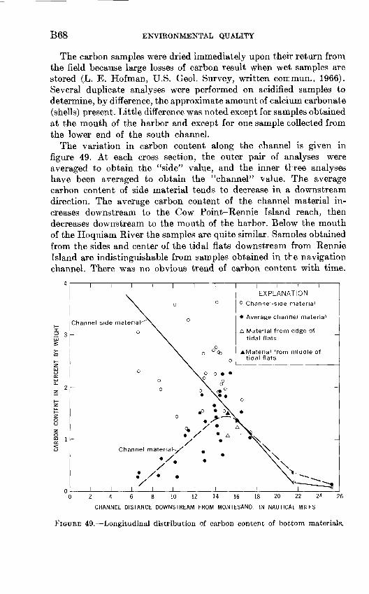
B68 ENVIRONMENTAL QUALITY
The carbon samples were dried immediately upon their return from the field because large losses of carbon result when wet samples are stored (L. E. Hofman, U.S. Geol. Survey, written com num., 1966). Several duplicate analyses were performed on acidified samples to determine, by difference, the approximate amount of calcium carbonate (shells) present. Little difference was noted except for samples obtained at the mouth of the harbor and except for one sample collected from the lower end of the south channel.
The variation in carbon content along the channel is given in figure 49. At each cross section, the outer pair of analyses were averaged to obtain the "side" value, and the inner three analyses have been averaged to obtain the "channel" value. The average carbon content of side material tends to decrease in a downstream direction. The average carbon content of the channel material in creases downstream to the Cow Point-Rennie Island reach, then decreases downstream to the mouth of the harbor. Below the mouth of the Hoquiam River the samples are quite similar. Samples obtained from the sides and center of the tidal flats downstream from Rennie Island are indistinguishable from samples obtained in tbe navigation channel. There was no obvious trend of carbon content with time.
S5 3
Channel-side material
I I I I
EXPLANATION
° Channel-side material
Average channel material
A Material from edge of tidal flats
^Material from middle of tidal flats
2 4 6 8 10 12 14 16 18 20 22 24
CHANNEL DISTANCE DOWNSTREAM FROM MONTESANO, IN NAUTICAL MILES
26
FIGURE 49. Longitudinal distribution of carbon content of bottom materials.

ESTUARINE STUDIES IN UPPER GRAYS HARBOR, WASH. B69
DISSOLVED OXYGEN DEMAND
The flow of the main channel transports the greatest amounts of solutes and organic detritus, materials that contribute tc the oxygen depletion of the water. There is a correlation between the decrease in dissolved oxygen of the water and the increase in carbon content of the bottom materials in the main channel. In figure 50, comparison is made between the longitudinal change in cr.rbon content of the bottom materials of the main channel (from fig. 49) and the 1965 average DO sag curve for low-flow, low-tide conditions (D. R. Fisher, Weyerhaeuser Co., written commun., 1966). The reach with the highest concentration of carbon in the bottom materials (Cow Point) also has the lowest concentration of dissolved oxygen in the overlying water. This reach is the primary area for deposition of organic detritus, including that transported into the estuary by the tributaries and that added by waste effluents.
Camp (1965, p. 10) estimated that half of the oxygen demand of the incoming detrital material in the Merrimack River estuary was satisfied before the material settled out. Camp's data, applied to Grays Harbor, suggest that a part of the total oxygen demand of the incoming organic detritus is "stored" in the bottom sediments. These deposits exert their demand slowly and therefore represent a potential demand. Should these materials be disturbed by dredging or in some manner mixed with harbor waters, the potential demand would become an immediate demand. An estimate of the potential BOD, taken as the COD (chemical oxygen demand), was therefore obtained for this investigation.
Several samples of bottom material collected in June and September 1966 were analyzed for COD by methods of the American Public Health Association (1960). The method was modified by allowirg the reagents and materials to stand at room temperature for about a week with occasional stirring, rather than refluxing. No chloride corrections were made, because the data are of a qualitative nature onl^. In figure 51, values of COD are plotted against concomitant carbon content. The COD generally increases with increasing carbon content, and the figure shows that there was evidently more oxidizable matter in the September samples than in the June samples. The COD reT ation agrees with data published elsewhere (Eriksen and Townsend, 1940; Thames Survey Committee and Water Pollution Research Labora tory, 1964).
The relation between carbon content and amount of fine material (organic-free material less than 0.062 mm) is shown in figure 52. Only average channel data were used to compute the regression line given.

B70 ENVIRONMENTAL QUALITY
I
£ 7
3 4
o 3
3 2
Low tide
J______I J____I____I
3 024 6 8 10 12 14 16 18 20
CHANNEL DISTANCE DOWNSTREAM FROM MONTESANO, IN NAUTICAL MILES
22
FIGURE 50. Comparison of longitudinal variations of carbon contert of channel- bottom materials and dissolved-oxygen content of harbor water. Carbon- content curve is from figure 49. Dissolved-oxygen curves are based on data for 1965 (D. R. Fisher, Weyerhaeuser Co., written commun., 196f).
The equation for the regression is:
(7=0.315+0.0238^, (17)

ESTTJARINE STUDIES IN UPPER GRAYS HARBOR, WASH. B71
160
140
E 120
100
80
60
40
20
o June 1966
September 1966
01234
CARBON CONTENT, IN PERCENT BY WEIGHT
FIGURE 51. Relation between chemical oxygen demand and carbon content ofbottom materials.
where C is the carbon content, in percent by dry weight, and F is percent, by weight, finer than 0.062 mm. The standard error c* esti mate is 0.463 percent carbon. The plot verifies the natural assumption that the fine material and organic material respond similarly to given depositional influences.
During the Thames River survey (Thames Survey Committee and Water Pollution Research Laboratory, 1964) bottom deposits were studied extensively for their physical and chemical composition and for the evolution of gas from these materials. The relation of carbon to fine material from the Thames River study (1964, p. 293) also is shown in figure 52. The upper curve, for the Thames reach above Mucking, was derived from data with more variability than those from the sea reach, the lower curve. The Grays Harbor regression line plots between the two Thames River lines.
As part of the Grays Harbor cooperative study, R. B. Herrmann (Weyerhaeuser Co., written commun., 1966) investigated the effect of tideflat materials (surficial algae) on the dissolved oxygen of overlying waters. Herrmann's studies indicated an apparent contri bution of oxygen by tidal flats during the summer. He estimated a net oxygen production of about 100 milligrams per square meter

B72 ENVIRONMENTAL QUALITY
\
/^-Thames River above Mucking
Main channel Grays Harbor
10 20 30 40 50 60 70
SEDIMENT FINER THAN 0.062 MILLIMETERS, IN PERCENT BY WEIGHT
80
FIGURE 52. Relation between carbon content and amount of fine sediment (less than 0.062 mm) for main channel bottom materials. Open circles indicate bottom samples obtained from main channel; solid circles indicate samples from south channel; and open triangles indicate samples from tidal flats. Dashed lines indicate similar relations for the Thames River, Great Britain (Thames Survey Committee and Water Pollution Research Laboratory, 1964, p. 293).
per hour from samples taken from the periphery of the tidal flats during the summer. This production rate must be applied to the average volume of overlying waters to compare the productivity with that of harbor waters. Westley (1967, p. 6) cit°-d a formula given by Westlake (1963): grams of oxygen multiplied by 0.3 equals grams of carbon. If this conversion factor is used, Herrmr.nn's estimate becomes about 0.07 milligram of oxygen per liter per hour at high tide, which is about double the productivity of harbor waters given by Westley and Tarr (1965).
Eriksen and Townsend (1940, p. 64-68) studied mud collected from the surface of Grays Harbor tidal flats and concluded that the

ESTUARINE STUDIES IN UPPER GRAYS HARBOR, WASH. B73
flats were "not responsible for the low dissolved-oxygen content of the water of upper Grays Harbor."
Other benefits from tidal flats might be shown. Langbein and Durum (1967), studying natural stream reaeration rates, found that:
where K2 is the reaeration coefficient, V is mean stream velocity, and H is the mean depth. Harbor waters move across the tidal flats during much of the tidal cycle, and thus, by providing a large moving surface area at shallow depth, should be credited with a large airount of the oxygen contribution. Additional oxygen is derived from the ocean winds that generally blow in this area. Air entrainment from waves over the shallows can only add to the dissolved oxygen.
Conversely, the potential oxygen demand of upper harbor bottom materials is fairly large. Dredging of large areas would stir up Quan tities of high-carbon sediment which could exert considerable demand at a period critical to harbor biota. An estimate of potential demand might be made by analyzing a series of core samples from an area to obtain an average carbon content and then converting this value to a potential oxygen demand using figure 51. Water running off dredge-spoil areas would be depleted of dissolved oxygen. However, unless disturbed, these deposits would probably have a relatively low oxygen demand.
During most low tides, the surface of Grays Harbor is broken, by many bubbles which are believed to have a scrubbing action on dis solved oxygen, removing it from solution as the bubbles rise through the water column. However, no evidence was collected to indicate this. The Thames Survey Committee and Water Pollution Research Laboratory (1964) discussed evolution of gases from bottom deposits. They determined 0.4-0.8 percent oxygen by volume in the bubbles of Tilbury tidal basin, Great Britain. Thus, presumably some scrubbing action also occurs in Grays Harbor.
SUMMARY OF BOTTOM MATERIALS
The influence of Grays Harbor bottom materials on the DC and BOD of harbor waters is complex. The segment of the estuary with bottom materials containing consistently high concentrations of organic carbon is in the vicinity of Cow Point. From the relation between carbon content and chemical oxygen demand, the bottom materials near Cow Point must exert some oxygen demand on the overlying waters. The organic carbon in bottom materials is found with fine particles (less than 0.062 mm in diameter), so the writers- con-

B74 ENVIRONMENTAL QUALITY
eluded that both are responding similarly to the depositional in fluences of higher salinity and water temperature, and slower velocity.
The tidal flats benefit the harbor waters moving across them. Herrmann's studies indicate a net oxygen production for the flats, and this production possibly offsets any deleterious effects of undisturbed channel materials. It is doubtful, however, if during a period of low fresh-water inflow, the benefit from the flats could ever offset the marked increase in potential oxygen demand caused by disturbing (by dredging) large areas of channel-bottom materials.
WATER QUALITY
The fresh, brackish, and oceanic waters in Grays Hsrbor are the habitats of many beneficial organisms, mostly shellfish ard salmonids. The salinity of the water defines the environment for most of these organisms, which are able to adapt to hydrologic and hydraulic changes in their environment; but the organisms are not usually able to adapt to water-quality changes in their environment. This section of the report describes the water-quality conditions r\ the upper harbor during the period of this study.
SALINITY
The first chemical characteristic of estuarine waters usually con sidered is salinity, or saltiness. Longitudinal salinity prof les in Grays Harbor (figs. 22-24) were presented earlier, in that part of the report dealing with dispersion coefficients. In the quasi-steady-«state model of an estuary, the longitudinal salinity distribution is considered to be in a dynamic equilibrium between the force of the fresh water on the system and the forces moving salts into the estuary. As the fresh water increases, water of a given salinity is found farther downstream. This is evident in figure 53, which shows the relation between fresh water discharge and the high-tide intrusion position of vTater with a salinity of 1 ppt (part per thousand) for 1966 field data (figs. 22-24). The 1-ppt intrusion point progresses farther inland with decreasing flow.
Salinity intrusion can also be measured at a fixed point in the harbor and related to hydraulic parameters, such as freeh-water dis charge and tidal stage. Two automatic water-quality monitors were installed in Grays Harbor for this project: one, owned by the Weyer haeuser Co., was installed on the Weyerhaeuser Co. dock at Cosmopo- lis, 8.9 miles downstream from Montesano and 19.5 miles upstream from the mouth; the second was installed at Hoquiam, 15.5 miles downstream from Montesano and 12.9 miles upstream from the mouth. These monitors continuously recorded water temperature, specific conductance, and dissolved oxygen. Sampling intakes were

ESTUARINE STUDIES IN UPPER GRAYS HARBOR, WASH. B75
10
ir
2 -
1-
300 1000
5-DAY AVERAGE FRESH-WATER DISCHARGE, IN CUBIC FEET PER SECOND
10,000
FIGURE 53. Relation between salinity intrusion and fresh-water discharge at high tides ranging from 6.5 to 11.5 feet. Anomalous point at 714 cfs is based on an estimated part of salinity curve (bottom graph of fig. 22).
attached to floats with the intake about 3 feet below the water sur face. Tidal stage was obtained with separate recorders.
An example of the information obtained at each monitor site is shown in figures 54 and 55. The upstream station, at Cosmopolis (fig. 54), recorded minimum conductivity and maximum dissolved-oxygen concentration at low tide, and the reverse at high tide. The down stream station, at Hoquiam (fig. 55), recorded minimum conductivity and minimum dissolved-oxygen content near low tide, and maximums near high tide. Minimum conductivities at Hoquiam are greate~ than the maximums at Cosrnopolis. Dissolved-oxygen concentrations at Hoquiam were less than those at Cosmopolis; peak values we:n only slightly greater than minimum values at Cosmopolis.

B76 ENVIRONMENTAL QUALITY
18
0400 0800 1200 1600 2000 2400
PACIFIC STANDARD TIME
FIGURE 54. Fluctuations of specific conductance, dissolved oxygen, and tidal stage at the Cosmopolis monitor on July 2, 1966. Fresh-wate~ discharge was 1,280 cfs, and water temperature ranged from 17° to 18°C. Dissolved-oxygen values are corrected for salinity.
Daily maximum conductivities at Cosmopolis for 620 days in the 1965 and 1966 calendar years were correlated with coincident fresh water discharge for this report by Pollution Control Commission personnel. The following regression equation was obtained:
#Cmax=76.4-17.7log10 Q/, (18)
where KCm&x is the specific conductivity, in millimhos at 25°C, and Qf is the fresh-water discharge, in cubic feet per second. The correla tion coefficient was 0.917, and the standard error of estimate was 4.25 millimhos. Evidently, variations in discharge cause most of the variations in the daily maximum conductivity at Cosmopolis. If a longitudinal salinity distribution function, such as eauation 5 or equation 9, is assumed, equation 18 can be used to estimate the location of water of a given salinity, or the intrusion point, for an

ESTUARINE STUDIES IN TIPPER GRAYS HARBOR, WASH. B77
32
30
o 28
26
24
22
20
18
16
14
12
100400 0800 1200 1600
PACIFIC STANDARD TIME
2400
FIGURE 55. Fluctuations of specific conductance, dissolved oxygen, and tidal stage at the Hoquiam monitor on July 2, 1966. Fresh-water discharge was 1,280 cfs, and water temperature ranged from 16° to 17°C. Dissolved-oxygen values are corrected for salinity.
assumed discharge. The equation for specific conductance can be converted roughly into salinity by using one of the following:
.563 (19)
where s\ is the salinity, in parts per thousand, and K is specific con ductivity less than 10.5 millimhos; or
s2 =0.643 #-0.81, (20)
where s2 is salinity for K greater than 10.5 millimhos. The two equa tions were derived from a conductivity-chloride relation for April 1965 field data (chloride analyses courtesy of D. R. Fisher, Weyer haeuser Co.) and substituted into an equation given by Sverdrup, Johnson, and Fleming (1942, p. 51):
§=0.03 + 1.805 chlorinity, (21)

B78 ENVIRONMENTAL QUALITY
where chlorinity was taken as the chloride concentration, in parts per thousand.
The upstream intrusion position of salts in an estuary is thus seen to be primarily a function of fresh-water discharge. This is because of the averaging of tidal forces over long periods. In the one- dimensional steady-state frame of reference, the salts are moved upstream by gravitational convection due to density differences and dispersion processes. Downstream movement is entirely due to the force of fresh-water discharge on the system. For constant Qf over a long period, an equilibrium condition should prevail, and intrusion should reach a specific point upstream.
DISSOLVED OXYGEN
In Grays Harbor, the characteristic of the water considered most important, and most affected by man, is the dissolved oxygen (Eriksen and Townsend, 1940, p. 36).
Many natural processes supply oxygen to harbor waters. Large amounts of oxygen are brought in by tributary streams and fresh ocean waters. The atmosphere supplies additional amounts of oxygen by entrainment due to the wind and waves and by reaeratior, Reaeration is the renewal of dissolved oxygen which takes place at a rate propor tional to the difference between the capacity and the actual content of dissolved oxygen of the harbor waters. Phytoplankton and periphyton usually have a net daily production of oxygen during critical summer months. However, Westley (1967) found a lower photosynthetic rate in the upper harbor which he ascribed primarily to turbidity and the presence of sulfite waste liquor. By comparing Grays Harbor with Willapa Bay, he estimated that upper Grays Harbor failed to receive about 0.17 mg/1 per day of dissolved oxygen owing to the lowered phytoplankton photosynthesis.
Another source of dissolved oxygen, usually neglected by investi gators, is precipitation. The 1931-60 average annual precipitation at Aberdeen was 84.5 inches (U.S. Weather Bureau, 1966, p. 231). On the order of 10 million pounds of dissolved oxygen would be supplied to the 99 square miles (statute) of Grays Harbor by this source annually if the DO concentration of the rain were estimated as 8 mg/1. How ever, for the same 1931-60 period, an average of only 7.01 inches of rain fell during July, August, and September, or an average of only 0.076 inch per day. On the basis of this value and an estimated DO content of 8 mg/1, about 9,000 pounds per day might be expected from precipitation during the low-flow period. This compares with an estimate of 22,000 pounds per day supplied by tributaries. Although not very large, the amount of dissolved oxygen carried by precipitation
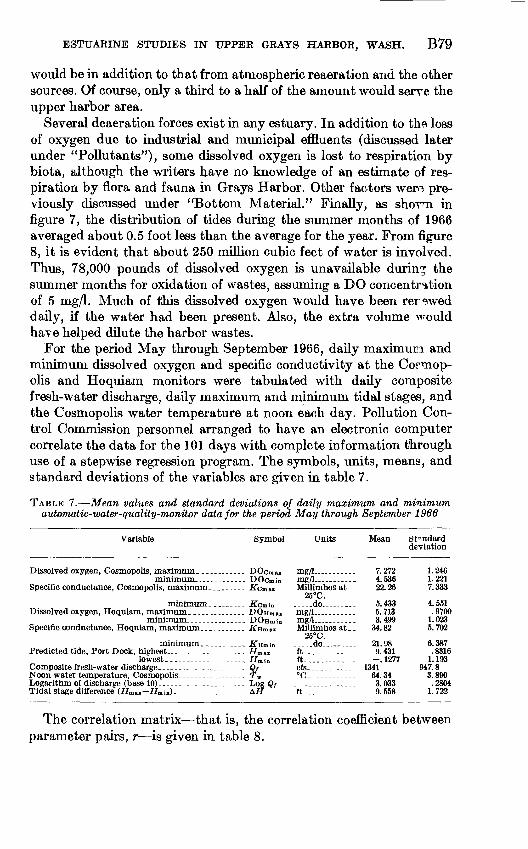
E3TUARINE STUDIES IN UPPER GRAYS HARBOR, WASH. B79
would be in addition to that from atmospheric reaeration and the other sources. Of course, only a third to a half of the amount would serve the upper harbor area.
Several deaeration forces exist in any estuary. In addition to the loss of oxygen due to industrial and municipal effluents (discussed later under "Pollutants"), some dissolved oxygen is lost to respiration by biota, although the writers have no knowledge of an estimate of res piration by flora and fauna in Grays Harbor. Other factors were pre viously discussed under "Bottom Material." Finally, as shorn in figure 7, the distribution of tides during the summer months of 1966 averaged about 0.5 foot less than the average for the year. From figure 8, it is evident that about 250 million cubic feet of water is involved. Thus, 78,000 pounds of dissolved oxygen is unavailable during the summer months for oxidation of wastes, assuming a DO concentration of 5 mg/1. Much of this dissolved oxygen would have been rerewed daily, if the water had been present. Also, the extra volume would have helped dilute the harbor wastes.
For the period May through September 1966, daily maximuEi and minimum dissolved oxygen and specific conductivity at the Cormop- olis and Hoquiam monitors were tabulated with daily composite fresh-water discharge, daily maximum and minimum tidal stages, and the Cosmopolis water temperature at noon each day. Pollution Con trol Commission personnel arranged to have an electronic computer correlate the data for the 101 days with complete information through use of a stepwise regression program. The symbols, units, means, and standard deviations of the variables are given in table 7.
TABLE 7. Mean values and standard deviations of daily maximum and minimum automatic-water-quality-monitor data for the period May through September 1966
Variable Symbol Units Mean Standarddeviation
Dissolved oxygen, Cosmopolis, maximum. .......minimum
Specific conductance, Cosmopolis, maximum.
minimum. _.-.Dissolved oxygen, Hoquiam, maximum.
minimum. ______ ...Specific conductance, Hoquiam, maximum.... _..
minimum...--..Predicted tide, Port Dock, highest. .. ............
lowest. --. _ ---.____.Composite fresh-water discharge- _ .... . ... Noon water temperature, Cosmopolis__ __ ... ...Logarithm of discharge (base 10)_-_-_-_-_. . ... Tidal stage difference (Hmn Hm i n)-.. ...........
..... DOcmax
.-._- DOcmin
-Kcmin.... DOHmw.---. DOHmin---- -firHm .x
KHm\n. _ - - - fi max
Hm -..... Q,
....LogQ,
mg/1.. .-.-.mg/1-.-.......Millimhos at
26°C..-.-.do ......mg/1.... . ...mg/1 ------Millimhos at . .
25°C......do -----ft-.......--...ft-.... ------CfS- _ . - °C---_ . ------
ft.............
7.2724.53622.26
5.4335.7133.499
34.82
21.989.431-. 1277
1341 64.343.0339.558
1.2461.2217.333
4.551.9700
1.0235.702
6.387.8316
1.193947.8
3.890.2804
1.722
The correlation matrix that is, the correlation coefficient between parameter pairs, r is given in table 8.

B80 ENVIRONMENTAL QUALITY
£
ss -e
^ s53
"8
5
S §1131i S
CO CO O O
CO «0 00 O
S o «nt^ IN
£* OO CO
^ OS t-~ OS O
S « S «n S
0 I
8 3? r
00B Bt0 0

ESTUARINE STUDIES IN UPPER GRAYS HARBOR, WASH. B81
For the 101 days, 0.165<r< + 0.165 is significant at the 10- percent level.
Daily minimum dissolved oxygen at Cosmopolis (DOCmin, in mg/1) was correlated with discharge (Qf), difference in tidal stage (AH), and daily minimum dissolved oxygen at Hoquiam (DOHmin) :
DOCmm=3.28+0.00094Q/, (22)= 6.03+0.00096(2,- 0.291 AH, (23)=4.28+0.0074Q,-0.212AH+0.369 DOHmin. (24)
From table 7, Qf is found to correlate significantly with DOHmin, which tends to negate the usefulness of equation 24. The correlation coeffi cients, r, and standard error of estimates, se, are:
Equation _ r_ se , in mg/122 0. 728 0. 84123 . 835 . 67824 . 868 . 616
With the same dependent variable, DOcmin, the correlation with daily minimum Hoquiam dissolved oxygen, DOHmin, and high tide, ffmax, gave the following:
DOCmin= 1.53+0.860 DOHm,n, (25) = 3.06+0.822 DOHm,n-0.149Hmax. (26)
Again, a fairly high correlation was found between the independent variables in the second equation. The r and se for these equations are :
Equation _ r_ se , in mg/125 0. 720 0. 85126 . 726 . 847
Similar correlations were made with Hoquiam daily minimum dissolved oxygen, DOHmin, as follows :
DOHmin=0.762+0.603DOCmin, (27)
=5.32-0.0826J^Hmin, (28)
= 7.66-0.0887^Hmm-0.232 AH, (29)
where .Kumin is t'he daily minimum specific conductance at Hoquiam. Fairly strong interdependence was again found among the inde-

B82 ENVIRONMENTAL QUALITY
pendent variables in the last equation. For these equations, r and se are:
Equation r se , in mg/1
27 0. 720 0.71328 . 516 .88029 . 646 .789
No correlations with waste loading were attempted. The effects of daily variations in effluent BOD and volume, however, are lessened by the decay properties of the materials. Because the efFuent compo nents require several days to oxidize completely, the longitudinal dissolved-oxygen curve represents the natural dissolved-oxygen profile with a time-integrated deficit from the wastes superimposed. In this report, then, the imposed effluent rate and its dissolved- oxygen demand are considered to be roughly constant as a first approximation.
As with salinity intrusion, if a typical longitudinal dissolved-oxygen distribution can be defined for Grays Harbor, correlation with perti nent parameters should allow estimation of the location, extent, and magnitude of the dissolved-oxygen minimum, or sag point. For instance, the average dissolved-oxygen curve shown in figure 50 is quite similar in form to the average curve for other years during low- flow periods (D. R. Fisher, Weyerhaeuser Co., written commun., 1966). Also, a fairly high correlation exists between characteristics of water in different areas of the harbor. This is borne out by the correla tion between maximum and minimum data at the Hoquiam monitor:
DOHmax=3.55+0.615DOH,nin, (30)
where DOHmax is the daily maximum dissolved oxygen at Hoquiam. The values of r and se for this equation are 0.652 and 0.739 mg/1 respectively. Therefore, given sufficient data related to a common time base, say, the equivalent half-tide position (The.mes Survey Committee and Water Pollution Research Laboratory, 1964, p. 7), the interrelation between water-quality characteristics in different areas of the harbor can be determined. Another possible common reference parameter might be the salinity or the chlorinity. When Elriksen and Townsend (1940, p. 45) plotted minimum dissolved oxygen versus chlorinity, they found that the minimum dissolved oxygen was almost invariably associated with chlorinities from 9 to 12. Converted to salinity, the range would be from 16 to 22 ppt.
The high degree of correlation between Cosmopolis and Hoquiam daily minimum dissolved oxygen in equations 25 and 27, however, only verifies the fact that the excursion of the water often allows

ESTUARINE STUDIES IN UPPER GRAYS HARBOR, WASH. P83
each monitor to sample the same water. Further corroboration of this is shown by the correlations between conductivities:
(31)(32)(33)
The following tabulation gives the respective r and se for each of the above equations:
Equation r se, in millimhos31 0.847 2.4332 .847 3.4133 .870 2.83
POLLUTANTS
The Pollution Control Commission (written commun., 1966) has tabulated the major sources of waste loading in Grays Harbor as part of their contribution to this cooperative study. The following is a summary of their tabulation:
BOD (Ibs Percent of total Effluent source per day) BOD load
Industrial:Rayonier, Inc. (pulp and paper)_______ 408. 000 89. 5Weyerhaeuser Co. (pulp) ______-. _ _ _ 45, 300 9. 96 lumber and plywood mills_________ 1, 240 . 3
Municipal:Aberdeen, Hoquiam, and Cosmopolis_ 1, 160 . 3
Other:5 fish companies (estimated) ___-__-___ 50 . 01
Total____-_-----_----._-----_-_-_ 455,750 100.01
Effluents from pulp and paper mills constitute by far the largest source of waste loading of the harbor. Of these effluents, the largest proportion of BOD is due to the sulfite waste liquor. Both pulpmills have continuing programs for reducing the BOD of their effluents, however, so that the tabular data applies only to conditions as of 1966.
Gunter and McKee (1960, p. 66) estimated that 90 percent of sulfite waste liquor will decompose within 10 days. They also noted that a typical 5-day BOD of undiluted sulfite waste liquor was about 30,000 mg/1 by weight. They also showed (1960, p. 65) an approximate gross analysis of sulfite waste liquor solids. Lignin sulfonic acids comprise 65.0 percent and fermentable sugars 15.0 percent of total solids. Analyses vary radically, depending on the process used, tree species, raw materials, and in-plant treatment.
Eriksen and Townsend (1940, p. 42-49) discussed the response of harbor waters to sulfite waste liquor. They found improvement in percent of saturation of dissolved oxygen within 4 days after mill

River
iee_at Montesano. __
Discharge (cfs)
588183
. _ _ _ 684
.___ 2.230
BOD(Ibs per day)
4,8201,5404,800
13. 200
DO(Ibs per day)
27, 7009,350
1. 500, 000
B84 ENVIRONMENTAL QUALITY
shutdown. In July 1939, the pulpmill was shut down for about 11 days, and the minimum DO climbed from 40 percent of saturation to 76 percent. Nine days after tjhe mill was restarted, the minimum DO was 27 percent of saturation; and a week later it was about 21 percent of saturation.
The Pollution Control Commission (written commun., 1966) also determined the approximate amount of dissolved oxygen brought into the upper harbor by tributary streams. The following table summarizes tributary contributions at intermediate flow:
Wishkah Hoquiam Wynoochee
Longitudinal BOD profiles of harbor waters obtained by the Weyerhaeuser Co. (D.R. Fisher, written commun., 1966, 1967) show that BOD values on the order of 0.5 mg/1 are typical of samples taken near Montesano and in the lower harbor. Maximum BOD values usually occur in the Cow Point reach at high tide and about half way down the south channel at low tide. The average of these maximum BOD values may be as high as 2 mg/1 with individual values as high as 4 mg/1.
The index of sulfite waste liquor, the Pearl-Benson index (PBI), has a similar longitudinal distribution. Values less than 10 mg/1 are found upstream and downstream in the upper harbor, whereas average values of almost 80 mg/1 are found around Cow Point at high tide and in the middle of the south channel at low tide. A few samples contained more than 100 mg/1 PBI.
The method of allocation of the dissolved-oxygen resources of an estuary need not be complicated: a good example was given by Waldichuk (1962, p. 29-31) for Alberni Harbor. In this example, the available dissolved oxygen of the harbor was related to the fresh water discharge. A second curve, computed from the first, related discharge to the dissolved oxygen remaining after satisfying the dissolved-oxygen requirement of the fishlife. Knowledge of the amount of dissolved oxygen required for stabilization of the pulpmill effluent then allowed determination of minimum discharge required or, alternatively, the maximum allowable dissolved-oxyger demand from the effluent.
SUMMARY OF WATER QUALITY
This section of the report has described some of the physical and chemical aspects of water quality of Grays Harbor. The extent of saline

ESTUARINE STUDIES IN UPPER GRAYS HARBOR, WASH. P85
intrusion at high tide was related to fresh-water discharge. With decreasing flow, water of a given salinity is found farther and farther inland. That this relationship exists is shown by equation 18. Dis charge is therefore the most important factor influencing salirity intrusion. Tidal forces evidently are averaged over long periods. Except for tidal mixing action, these forces are of minor importance in substantially influencing the maximum extent of the intrusior.
Dissolved oxygen is the most important water-quality parameter in Grays Harbor when consideration is given to the entire biolog; cal community man, fowl, fish, and shellfish. The natural fluctuation of dissolved oxygen, high in the winter and low in the summer, coincides with the fluctuation of fresh-water inflow and of water temperature. The supply of dissolved oxygen in harbor waters is renewed only by natural processes which are subject to the usual vagaries of nature. The supply of dissolved oxygen is lowest during the summer, low-f ow months, and it is diminished still further by industrial wastes. Further more, a decrease in the tidal volume during this low-flow period re duces the amount of oxygen available for stabilizing these wastes and also reduces the amount of water available for diluting them.
The similarity of successive dissolved-oxygen-sag curves obtained over a period of years makes possible the monitoring of the dissolved oxygen minimum with a single instrument placed between the limits of excursion of that minimum. With this instrument, the disposal of industrial wastes could be scheduled to minimize the depletior of dissolved oxygen.
Essentially then, the problem facing water-resources management in Grays Harbor is the selection of a suitable compromise between the needs of the entire biological community (from man to the lowest plankton) and the wastes discharged into the water environment.
The allocation to various uses of the water-quality resource? of Grays Harbor, especially the dissolved oxygen, is the responsibility of management. After the allocation of the dissolved-oxygen resources to the biota and for stabilization of wastes, a reserve of dissolved oxygen would seem essential in the event of natural or accidental disasters.
The information in this report should assist management personnel in obtaining a greater understanding of the influences on the water quality of upper Grays Harbor.
REFERENCES CITEDAmerican Public Health Association, 1960, Standard methods for examination
of water and wastewater [llth ed.]: New York, 626 p. Bader, R. G., McLellan, P. M., and others, 1955, Grays Harbor, Washing-ton,
a literature survey: Seattle, Washington Univ. Dept. Oceanography, 142 p.

B86 ENVIRONMENTAL QUALITY
Bialkowsky, H. W., and Billington, P. S., 1957, Pilot studies to predict effectsof waste on receiving waters: Sewage and Indus. Wastes, v. 29, no. 5, p. 551-569.
Budinger, T. F., Coachman, L. K., and Barnes, C. A., 1964, Columbia Rivereffluent in the northeast Pacific Ocean, 1961, 1962 Selected aspects ofphysical oceanography: Seattle, Washington Univ. Dept. OceanographyTech. Kept. 99, 78 p.
Camp, T. R., 1965, Field estimates of oxygen balance parameters: Am. Soc.Civil Engineers Proc., Sanitary Eng. Div. Jour., v. 91, no. FA5, p. 1-16.
Diachishin, A. N., 1963a, Dye dispersion studies: Am. Soc. Civil EngineersProc., Sanitary Eng. Div. Jour., v. 89, no. SAl, p. 29-49.
1963b, Waste disposal in tidal waters: Am. Soc. Civil Engineers Proc., Sanitary Eng. Div. Jour., v. 89, no. SA4, p. 23-43.
Eriksen, A., and Townsend, L. D., 1940, The occurrence and cause of pollution in Grays Harbor: Olympia, Washington State Pollution Control Comm., Pollution Ser., Bull. 2, 100 p.
Federal Inter-Agency Committee on Water Resources, Subcoirmittee on Sedi mentation, 1957, The development and calibration of the visual-accumula tion tube, rept. 11 in A study of methods used in measurement and analysis of sediment loads in streams: U.S. Govt. Printing Office, 1C° p.
1958, Operation and maintenance of U.S. BM-54 bed-material sampler: U.S. Govt. Printing Office, rept. M, 14 p.
1963, Determination of fluvial sediment discharge, rept. 14 in A studyof methods used in measurement and analysis of sediment Hads in streams:U.S. Govt. Printing Office, 151 p.
Gilbert, G. K., 1917, Hydraulic-mining debris in the Sierra Nevada: U.S. Geol.Survey Prof. Paper 105, 154 p.
Gross, M. G., and Nelson J. L., 1966, Sediment movement on the continentalshelf near Washington and Oregon: Science, v. 154, p. 879-880, 885.
Gunter, Gordon, and McKee, J. E., 1960, On oysters and sulfHe waste liquor:Olympia, Wasington State Pollution Control Comm., Spec. ConsultantsRept., 93 p.
Ippen, A. T., and Harleman, D. R. F., 1961, One-dimensional analysis of salinityintrusion in estuaries: Vicksburg, Miss., U.S. Army Corps Engineers Comm.Tidal Hydraulics Tech. Bull. 5, 55 p.
Keighton, W. B., 1966, Fresh-water discharge-salinity relations in the tidalDelaware River: U.S. Geol. Survey Water-Supply Paper 15^6-G, 16 p.
Ketchum, B. H., 1951a, The flushing of tidal estuaries: Sewage and Indus.Wastes, v. 23, no. 2, p. 198-209.
195Ib, The exchanges of fresh and salt waters in tidal estuaries: Jour.Marine Research, v. 10, no. 1, p. 18-38.
Langbein, W. B., and Durum, W. H., 1967, The aeration capacity of streams:U.S. Geol. Survey Giro. 542, 6 p.
Miller, E. G., 1962, Observations of tidal flow in the Delaware River: U.S.Geol. Survey Water-Supply Paper 1586-C, 26 p.
O'Connor, D. J., 1961, Oxygen balance of an estuary: Am. Soc. Civil EngineersTrans., v. 126, pt. 3, p. 556-576, with closure, p. 602-611.
1965, Estuarine distribution of nonconservative substances: Am. Soc Civil Engineers Proc., Sanitary Eng. Div. Jour., v. 91, no. SAl, p. 23-42.
Orlob, G. T., Jones, K. R., and Peterson, D. R., 1951, An investigation of domestic and industrial waste pollution in the lower Chehalis River and Grays Harbor: Olympia, Washington State Pollution Control Comm. Tech. Bull. 6, 50 p.

ESTUARESTE STUDIES IN UPPER GRAYS HARBOR, WASH. P87
Pearson, E. A., and Holt, G. A., I960, Water quality and upwelling at GraysHarbor entrance: Limnology and Oceanography, v. 5, no. 1, p. 48-56.
Peterson, D. R., 1953, Sewage pollution in the estuarial river areas of G~aysHarbor: Olympia, Washington State Pollution Control Comm. Tech. Pull.16, 17 p.
Peterson, D. R., Wagner, R. A., and Livingston, A., 1957, A re-investigation ofpollution in the lower Chehalis River and Grays Harbor (1956-1557):Olympia, Washington State Pollution Control Comm. Tech. Bull. 21, £2 p.
Richardson, D., 1962, Drainage-area data for western Washington: U.S. Geol.Survey open-file report, 244 p.
Schultz, E. A., and Simmons, H. B., 1957, Fresh water-salt water density currents,a major cause of siltation in estuaries: Vicksburg, Miss., U.S. Army CorpsEngineers Comm. Tidal Hydraulics Tech. Bull. 2, 28 p.
Stelzenmuller, W. B., 1965, Tidal characteristics of two estuaries in Florida:Am. Soc. Civil Engineers Proc,, Waterways and Harbors Div. Jour., v. 91,no. WW3, p. 25-36.
Stommel, H., 1953, Computation of pollution in a vertically mixed estuary:Sewage and Indus. Wastes, v. 25, no. 9, p. 1065-1071.
Sverdrup, H. U., Johnson, M. W., and Fleming, R. H., 1942, The oceans: Engle-wood Cliffs, N.J., Prentice Hall, Inc., 1087 p.
Thames Survey Committee and Water Pollution Research Laboratory, 1964,Effects of polluting discharges on the Thames Estuary: London, Dept. Sci.and Indus. Research, Water Poll. Research Tech. Paper 11, 609 p.
U.S. Coast and Geodetic Survey, 1958, Tidal bench marks, Point Chehalis andvicinity, Grays Harbor: U.S. Coast and Geod. Survey, Washington 33, 2 p.
1965, Tidal bench marks, Aberdeen, Grays Harbor: U.S. Coast and Geod.Survey, Washington 36, 2 p.
-1965, Tide tables, high and low water predictions, west coast of Northand South America, 1966: U.S. Govt. Printing Office, published annually.
U.S. Weather Bureau, 1966, Climatological data, Washington, 1965 annual sum mary: U.S. Weather Bur., v. 69, no. 13, p. 231.
Waldichuk, Michael, 1962, Some water pollution problems connected with dis posal of pulp mill wastes: The Canadian Fish Culturist, Issue 31, p. 3-34.
1966, Effects of sulfite wastes in a partially enclosed marine syste*n in British Columbia: Water Pollution Control Federation Jour., v. 38, EO. 9, p. 1484-1505.
Westlake, D. F., 1963, Comparisons of plant productivity: Biol. Rev., v. 38, p. 385-425.
Westley, R. E., 1967, Phytoplankton photosynthesis and its relationship to oxygen in Grays Harbor, Washington: Washington State Dept. Fisheries, Research Div., 30 p.
Westley, R. E., and Tarr, M. A., 1965, Physical-chemical and primary prodv^tiv- ity data, Grays Harbor, Hydrographic Trips 8-12, 1964 and 1965, in Hydro- graphic Data: Washington State Dept. Fisheries, v. 5, no. 1, 25 p.

INDEX
[Italic page numbers indicate major references]
Aberdeen, precipitation....._.............. B8,78tidal range....-.--.__....___.......
Abstract__._......................_....Acknowledgments............................Algae, effect on dissolved oxygen.__._..___.__Analyses, bottom materials, carbon content..
bottom materials, particle size, coarsefraction_.......................
particle size, fine fraction._____ _ _____
Bottom materials, carbon content------------sampling..--.--.-.-.-.-...-.......-----..sedimentation, _________._______.___._....size analyses, coarse fraction..............
fine fraction.-------------------------summary - --------------.._.------_-_-----
Bottom water, movement....................Bubbles, scrubbing action on dissolved
oxygen.__________________________
Carbon content, relation to amount of fine material, regression equation...............
Carbon content of bottom materials. -...-....relation to dissolved oxygen content in
water_.........................Chehalis River, at Porter, discharge..........
largest tributary to harbor-...............salt-water intrusion.... ...................
Conductivity of water, regression equation... Cosmopolis, water-quality monitor...........Correlation matrices for water-quality data... Cow Point, carbon content of bottom mate
rials--...-.-.-.......---------..-.
76
16767480
73pollution..----.---._---.----..__--... 84
Cross-sectional area of estuary, at mean tidelevel, equation.._-_.----_-_-._ 26
D ifferential movement of water layers........ 18Differential transport, defined.-_ -- ._ _._ 29Diffusion, defined_......................... 28Diffusivity coefficients, relation to discharge.. 54Discharge, principal streams ............... 7
relation to excursion distance............. 48Dispersion coefficients, computation.......... 51
use...------.---...-..--.-.--.-------...-. 56Dissolved oxygen, critical level............... 5
daily minimum, correlation.____.__._.__ 81deaeration forces_....................... 79demand---.-------.---.----..------.-.-.- 69effect of sulfite waste liquor............... 83scrubbing action by bubbles.............. 73sources-..-.................-.------.----. 78
Diurnal tidal range, defined.............__ B12Dredging, effect on dissolved oxygen demand.. 69,73
effect on water quality__.-.----...--.-. 58Dye studies_............................... 41
Equation, cross-sectional area of estuary at mean low water--.---..-._.....
cross-sectional area of estuary at mean tide level.___._..._.._..
fresh-water velocity__--.-.._--.------.-longitudinal salinity distribution. --------mean velocity at mean low water-...-....reaeration rate.--------------....------.--regression, carbon content and amount
of fine material in sediment.......conductivity.........................
specific conductance to salinity conver sion. ---.-.---.-.-.----.------.---
traveltime- ...............................turbulent transport coefficient ............
Estuary geometry, relation to excursion dis tance......... -_-_ _- ----------
Excursion distances.___.__..__ ....-_ ---factors affecting.-..-----.------- ------in tidal cycle..-_ - ..- summary...-.--.------------------- ------
26
2628313773
7076
774137
4941,50
454355
21038
638,40
Fish kills................-----------Flow-duration curves...----------------Flushing time, mean, estimation. _._... Fresh water.____.. .. ---- ---------
mean age ---------------------------
Geographic setting-.-... -------- ----- 2
Harleman, D. R. F., and Ippen, A. T., model for longitudinal salinity distri bution _.....-.---------.-------- 31
Hoquiam, water-quality monitor............. 74
Industry... ------------------------------- 2Intertidal volume...------------------------- 31
defined..------- ......- . - ------ 13Ippen, A. T., and Harleman, D. R. F., model
for longitudinal salinity distribu tion..------------------------- 31
Ketchum, B. H., longitudinal salinity dis tribution.--------------------- 30
Low flow, occurrence.. . .. -- 10,12
Mean age of fresh water.-...-.--------- ---- 38in terms of traveltime--..-- ------- -- 40
Mean tidal prism ....... ..- - ---- 31
B89

BOO INDEX
Mean tidal range, defined. Montesano, tidal range....
Net movement of estuarine waters.
PageB12
12
26
Oxygen production, tideflats. 71
Paper mills, pollutants..... Pearl-Benson index __. Point Chehalis, tidal range.
tidal reference planes... Pollutants, dissipation rate.
rate of removal, factors.sources....-.--...--.....---... _...
Pollution Control Commission, role in study- Pollution problem______________. Precipitation, at Aberdeen......---..-__..Present investigation..._..-....-_--......Previous investigations..-...------- .......Pulpmills, pollutants ..._ .
Reaeration rate, natural streams- References cited.
Salinity, computed from specific conductance. defined... --.----- -----------------distribution... ....--..--.-----__...relation to fresh-water discharge..........relation to sedimentation...__._. -._____
Salt-water intrusion, Chehalis River--.......relation to discharge. _----------------
Sampling, bottom materials.. _..._-.___ _dye studies-------__.................
Satsop River, at Satsop, discharge............Sediments, factors affecting deposition........Separation distance, concept ..-_........Sloughs, excursion distances..----.-___..
Page Streams, tributary to Grays Farbor, drainage
areas _____________ B7 Sulflte waste liquor______________ 83
Temperature of water, relation to sedimenta tion__..........__.___.. 57
Thames River survey...___________ 71Tidal flats, area.............................. 13
benefit to harbor waters_________ 74Tidal influence, limit defined. ............. 16Tidal range, relation to excurs'on distance. _ 47Tidal reference planes, Point Chehalis........ 12Tidal separation distances__________ 26Tideflat materials, effect on dissolved oxygen. 71Tides. , - -... ...... .....--- ItTraveltime, dye studies...._________ 46
mean age in tidal cycles.-.._.-..__.. 40Tributaries, excursion distances.-__..__. 50Turbulent transport coefficient___.____ 37
Upwelling, coastal.
Velocity of water, in estuary_.......maximum mean, in upper harbor.maximum mean tidal__...__.relation to sedimentation. __. _
Vertical salinity gradient.............Volume of upper harbor..._........
Washington State Department of Fisheries, role in study-__.__. ._.
Washington State Department of Game, role in study..__...___..__
Water quality.....--.-..__.__....__.. summary__..._....__..._...._..
Weyerhaeuser Co., role in studv_--------...Wynoochee River, above Srve Creek, dis-
charge..____..._-...-.......
6
171753572914
47484
4
U.S. GOVERNMENT PRINTING OFFICE : 1969 O-322-777