estimation of seasonal precipitation tercile-based

Estimation of Seasonal Precipitation Tercile-Based Categorical Probabilitiesfrom Ensembles

MICHAEL K. TIPPETT, ANTHONY G. BARNSTON, AND ANDREW W. ROBERTSON

International Research Institute for Climate and Society, Columbia University, Palisades, New York

(Manuscript received 23 November 2005, in final form 18 September 2006)

ABSTRACT

Ensemble simulations and forecasts provide probabilistic information about the inherently uncertainclimate system. Counting the number of ensemble members in a category is a simple nonparametric methodof using an ensemble to assign categorical probabilities. Parametric methods of assigning quantile-basedcategorical probabilities include distribution fitting and generalized linear regression. Here the accuracy ofcounting and parametric estimates of tercile category probabilities is compared. The methods are firstcompared in an idealized setting where analytical results show how ensemble size and level of predictabilitycontrol the accuracy of both methods. The authors also show how categorical probability estimate errorsdegrade the rank probability skill score. The analytical results provide a good description of the behaviorof the methods applied to seasonal precipitation from a 53-yr, 79-member ensemble of general circulationmodel simulations. Parametric estimates of seasonal precipitation tercile category probabilities are gener-ally more accurate than the counting estimate. In addition to determining the relative accuracies of thedifferent methods, the analysis quantifies the relative importance of the ensemble mean and variance indetermining tercile probabilities. Ensemble variance is shown to be a weak factor in determining seasonalprecipitation probabilities, meaning that differences between the tercile probabilities and the equal-oddsprobabilities are due mainly to shifts of the forecast mean away from its climatological value.

1. Introduction

Seasonal climate forecasts are necessarily probabilis-tic, and forecast information is most completely char-acterized by a probability density function (pdf). Esti-mation of the forecast pdf is required to measure pre-dictability and to issue accurate forecasts. For reliableforecasts, the difference between the climatological andforecast pdfs represents predictability, and several mea-sures of this difference have been developed to quantifypredictability (Kleeman 2002; DelSole 2004; Tippett etal. 2004; DelSole and Tippett 2007). Quantile probabili-ties are the probabilities assigned to quantile-delimitedcategories and provide a coarse-grained description ofthe forecast and climatological pdfs, which is appropri-ate for ensembles with relatively few members. TheInternational Research Institute for Climate and Soci-

ety (IRI) issues seasonal forecasts of precipitation andtemperature in the form of tercile-based categoricalprobabilities (hereafter called tercile probabilities),that is, the probability of the below-normal, normal,and above-normal categories (Barnston et al. 2003).Forecasts that differ from equal-odds probabilities, tothe extent that they are reliable, are indications of pre-dictability in the climate system. Accurate estimation ofquantile probabilities is important both for quantifyingseasonal predictability and for making climate fore-casts.

In single-tier seasonal climate forecasts, initial condi-tions of the ocean–land–atmosphere system are thesource of predictability, and ensembles of coupledmodel forecasts provide samples of the model atmo-sphere–land–ocean system evolution consistent withthe initial conditions, their uncertainty, and the internalvariability of the coupled model. In two-tier seasonalforecasts, ensembles of atmospheric general circulationmodels (GCMs) provide samples of equally likelymodel atmospheric responses to a particular configura-tion of sea surface temperature (SST). Tercile prob-abilities must be estimated from finite ensembles in ei-

Corresponding author address: M. K. Tippett, International Re-search Institute for Climate and Society, The Earth Institute ofColumbia University, Lamont Campus/61 Route 9W, Palisades,NY 10964.E-mail: [email protected]

2210 J O U R N A L O F C L I M A T E VOLUME 20

DOI: 10.1175/JCLI4108.1

© 2007 American Meteorological Society

JCLI4108

ther system. A simple nonparametric estimate of thetercile probabilities is the fraction of ensemble mem-bers in each category. Alternatively, the entire forecastpdf including tercile probabilities can be estimated bymodeling the ensemble as a sample from an analyticalpdf with adjustable parameters for mean, spread, shape,etc. Here we use a Gaussian distribution described byits mean and variance. The counting method has theadvantage of making no assumptions about the form ofthe forecast pdf. Both approaches are affected by sam-pling error due to finite ensemble size, though to dif-ferent degrees. This paper is about the impact of sam-pling error on parametric and nonparametric estimatesof simulated and forecast tercile probabilities for sea-sonal precipitation totals. We analyze precipitation be-cause of its societal importance and because, even onseasonal time scales, its distribution is farther from be-ing Gaussian, and hence more challenging to describe,than quantities like temperature and geopotentialheight, which have been previously examined.

In this paper we present analytical descriptions of theaccuracy of the counting and Gaussian tercile probabil-ity estimators. These analytical results facilitate thecomparison of the counting and Gaussian estimates andshow how the accuracy of the estimators increases asensemble size and predictability level increase. Theanalytical results support previous empirical resultsshowing the advantage of the parametric estimators.Wilks (2002) found that modeling numerical weatherprediction ensembles with Gaussian or Gaussian mix-ture distributions gave more accurate estimations ofquantile values than counting, especially for quantilesnear the extremes of the distribution. Kharin andZwiers (2003) used Monte Carlo simulations to showthat a Gaussian fit estimate was more accurate thancounting for Gaussian distributed forecast variables.

We show how the accuracy of the tercile probabilityestimates affects the rank probability skill score(RPSS). The RPSS is a multicategory generalization ofthe two-category Brier skill score. Richardson (2001)found that finite ensemble size had an adverse effect onthe Brier skill score with low-skill regions being morenegatively affected by small ensemble size. Changes inensemble size that cause only modest changes in Brierskill score can lead to large changes in economic valueimplied by a simple cost–loss decision model, particu-larly for extreme events (Richardson 2001).

Accurate estimation of tercile probabilities fromGCM ensembles does not ensure a skillful simulationor forecast if there are systematic errors in the GCMpdf. Calibration of model probabilities is needed to ac-count for model deficiencies and produce reliable cli-mate forecasts (Robertson et al. 2004). We expect that

forecast skill would be improved by reducing samplingerror in the GCM probabilities that are inputs to boththe calibration system and the procedure to estimatecalibration parameters. We investigate the roles of sam-pling and model error using a 79-member ensemble ofGCM simulations of seasonal precipitation made withobserved SST; we examine the impact of reducing sam-pling error on the skill of the simulations with and with-out calibration. Additionally, we use the GCM data toassess the importance of some simplifying assumptionsused in the calculation of the analytical results by com-paring the analytical results with empirical ones ob-tained by subsampling from the large ensemble ofGCM simulations.

An important predictability issue relevant to para-metric estimation of tercile probabilities is the relativeroles of the forecast mean and variance in determiningpredictability (Kleeman 2002). Since predictability is ameasure of the difference between forecast and clima-tological distributions, identifying the parameters asso-ciated with predictability also identifies the parametersthat are useful for estimating tercile probabilities. Forinstance, if the predictability of a system is due to onlythe changes in the forecast mean, then the forecastmean should also be useful for estimating tercile prob-abilities. One approach to this question is to identify theparameters that give the most skillful forecast prob-abilities (Buizza and Palmer 1998; Atger 1999). Kharinand Zwiers (2003) showed that the Brier skill score ofhindcasts of 700-mb temperature and 500-mb heightwas improved when probabilities were estimated froma Gaussian distribution with constant variance as com-pared with counting; fitting a Gaussian distributionwith time-varying variance gave inferior results. Hamillet al. (2004) used a generalized linear model (GLM;logistic regression) to estimate forecast tercile prob-abilities of 6–10 day and week-2 surface temperatureand precipitation and found that the ensemble variancewas not a useful predictor of tercile probabilities. Inaddition to looking at skill, we examine the relativeimportance of the forecast mean and variance for pre-dictability in the perfect model setting by asking wheth-er including ensemble variance in the Gaussian esti-mate and the GLM estimate reduces sampling error.

The paper is organized as follows. The GCM andobservation data are described in section 2. In section 3,we derive some theoretical results about the relativesize of the error of the counting and fitting estimatesand about the effect of sampling error on the rankedprobability skill score. The GLM is also introduced andrelated to Gaussian fitting. In section 4, we compare theanalytical results with empirical GCM-based ones and

15 MAY 2007 T I P P E T T E T A L . 2211

include effects of model error. A summary and conclu-sions are given in section 5.

2. Data

Model-simulated precipitation data come from a 79-member ensemble of T42 ECHAM4.5 GCM (Roeck-ner et al. 1996) simulations forced with observed SSTfor the period December 1950 to February 2003. Weuse seasonal averages of the 3-month period Decemberthrough February (DJF), a period when ENSO is asignificant source of predictability. We consider all landpoints between 55°S and 70°N, including regions whosedry season occurs in DJF and where forecasts are notusually made. While the results here use unprocessedmodel-simulated precipitation, many of the calculationswere repeated using Box–Cox transformed data. TheBox–Cox transformation

xBC � ��1�x� � 1�, � � 0

logx, � � 0�1�

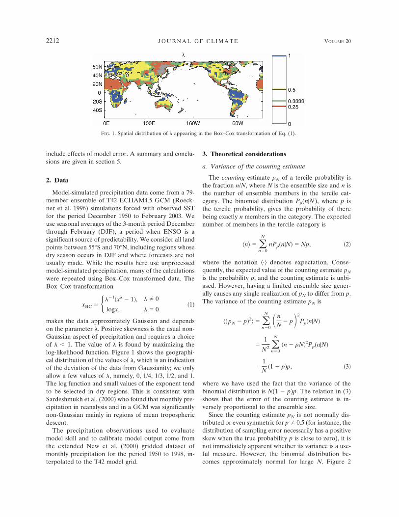
makes the data approximately Gaussian and dependson the parameter �. Positive skewness is the usual non-Gaussian aspect of precipitation and requires a choiceof � � 1. The value of � is found by maximizing thelog-likelihood function. Figure 1 shows the geographi-cal distribution of the values of �, which is an indicationof the deviation of the data from Gaussianity; we onlyallow a few values of �, namely, 0, 1/4, 1/3, 1/2, and 1.The log function and small values of the exponent tendto be selected in dry regions. This is consistent withSardeshmukh et al. (2000) who found that monthly pre-cipitation in reanalysis and in a GCM was significantlynon-Gaussian mainly in regions of mean troposphericdescent.

The precipitation observations used to evaluatemodel skill and to calibrate model output come fromthe extended New et al. (2000) gridded dataset ofmonthly precipitation for the period 1950 to 1998, in-terpolated to the T42 model grid.

3. Theoretical considerations

a. Variance of the counting estimate

The counting estimate pN of a tercile probability isthe fraction n/N, where N is the ensemble size and n isthe number of ensemble members in the tercile cat-egory. The binomial distribution Pp(n|N), where p isthe tercile probability, gives the probability of therebeing exactly n members in the category. The expectednumber of members in the tercile category is

�n� � n�0

N

nPp�n|N� � Np, �2�

where the notation �·� denotes expectation. Conse-quently, the expected value of the counting estimate pN

is the probability p, and the counting estimate is unbi-ased. However, having a limited ensemble size gener-ally causes any single realization of pN to differ from p.The variance of the counting estimate pN is

��pN � p�2� � n�0

N � n

N� p�2

Pp�n|N�

�1

N2 n�0

N

�n � pN�2Pp�n|N�

�1N

�1 � p�p, �3�

where we have used the fact that the variance of thebinomial distribution is N(1 � p)p. The relation in (3)shows that the error of the counting estimate is in-versely proportional to the ensemble size.

Since the counting estimate pN is not normally dis-tributed or even symmetric for p 0.5 (for instance, thedistribution of sampling error necessarily has a positiveskew when the true probability p is close to zero), it isnot immediately apparent whether its variance is a use-ful measure. However, the binomial distribution be-comes approximately normal for large N. Figure 2

FIG. 1. Spatial distribution of � appearing in the Box–Cox transformation of Eq. (1).


Fig 1 live 4/C

shows that the standard deviation gives a good estimateof the 16th and 84th percentiles of pN for p � 1/3 andmodest values of N. In this case, the counting estimatevariance is (2/9)N. The percentiles are obtained by in-verting the cumulative distribution function of thesample error. Since the binomial cumulative distribu-tion is discrete, we show the smallest value at which itexceeds 0.16 and 0.84. Figure 2 also shows that for mod-est-sized ensembles (N � 20) the standard deviation isfairly insensitive to incremental changes in ensemblesize; increasing the ensemble size by a factor of 4 isnecessary to reduce the standard deviation by a factorof 2.

The average variance of the counting estimate for anumber of forecasts is found by averaging (3) over thevalues of the probability p. The extent to which theforecast probability differs from the climatologicalvalue of 1/3 is an indication of predictability, with largerdeviations indicating more predictability. Intuitively,we expect regions and seasons with more predictabilityto suffer less from sampling error on average since en-hanced predictability implies more reproducibilityamong ensemble members. In fact, when the forecastdistribution is Gaussian with mean �f and variance f,the variance of the counting estimate of the below-normal category probability is (see the appendix fordetails)

��pN � p�2� �1N

�1 � p�p

�1

4N�1 � �erf�xb � �f

�2�f��2�, �4�

where xb is the left tercile boundary and erf denotes theerror function. Since the absolute value of the errorfunction approaches unity when the absolute value ofits argument is large, the counting estimate variance issmall when the ensemble mean is large or the ensemblevariance is small. Assuming that the forecast variance f is constant and averaging (4) over forecasts gives thatthe average variance is approximately (see the appen-dix for details)

��pN � p�2� �1N��1 � p�p�

� �0.0421868

N�

0.264409

N�1 � S2

�2

9N�1 � S2, �5�

where S2 is the usual signal-to-noise ratio [see (A4);Kleeman and Moore (1999); Sardeshmukh et al.(2000)]. When there is no skill S � 0, p � 1/3, and theaverage variance is (2/9)N. The signal-to-noise ratio isrelated to correlation skill with r � S/�1 � S2 beingthe expected correlation of the ensemble mean with anensemble member. The relation in (5) has the practicalvalue of providing a simple estimate of the ensemblesize needed to achieve a given level of accuracy for thecounting estimate of the tercile probability. This value,like the signal-to-noise ratio, depends on the model,season, and region.

b. Variance of the Gaussian fit estimate

Fitting a distribution with a few adjustable param-eters to the ensemble values is an alternative method ofestimating a quantile probability. Here we use a Gaus-sian distribution with two parameters, mean and vari-ance, for simplicity and because it can be generalized tomore dimensions (Wilks 2002). The Gaussian fit esti-mate gN of the tercile probabilities is found by fittingthe N-member ensemble with a Gaussian distributionand integrating the distribution between the climato-logical tercile boundaries (Kharin and Zwiers 2003).The Gaussian fit estimate has two sources of error: (i)the non-Gaussianity of the forecast distribution fromwhich the ensemble is sampled and (ii) sampling errorin the estimates of mean and variance due to limitedensemble size. The first source of error is problem de-pendent, and we will quantify its impact empirically forthe case of GCM-simulated seasonal precipitation. Thevariance of the Gaussian fit estimate can be quantifiedanalytically for Gaussian distributed variables. When

FIG. 2. The 16th and 84th percentiles (see text for details) of thecounting estimate pN (solid lines) and p plus and minus the stan-dard deviation of the estimate pN (dashed lines) for p � 1/3 (dot-ted line).

15 MAY 2007 T I P P E T T E T A L . 2213

the forecast distribution is Gaussian with mean �f andknown variance f, the variance of the Gaussian fit es-timate of the below-normal category probability is ap-proximately (see the appendix for details)

�gN � p�2 �1

2�Nexp��xb � �f

�f�2�, �6�

where xb is the left tercile boundary. The average (overforecasts) variance of the Gaussian fit tercile probabil-ity is approximately (see appendix for details)

��gN � p�2� �

exp��1 � S2

1 � 2S2 x02�

2�N�1 � 2S2, �7�

where x0 � ��1(1/3) � �0.4307 and � is normal cu-mulative distribution function. Comparing this valuewith the counting estimate variance in (5) shows thatthe Gaussian fit estimate has smaller variance for allvalues of S2, with its advantage over the counting esti-mate increasing slightly as the signal-to-noise ratio in-creases to levels exceeding unity.

When there is no predictability (S � 0), the averagevariance of the Gaussian fit is

��gN � p�2� �e�x0

2

2�N�

0.1322N

�8�

and depends only on ensemble size. Comparing (3) and(8), we see that the variance of the Gaussian estimatedtercile probability is about 40% smaller than that of thecounting estimate if the ensemble distribution is indeedGaussian with known variance and no signal (S � 0).The inverse dependence of the variances on ensemblesize means that modest decreases in variance areequivalent to substantial increases in ensemble size. Forinstance, the variance of a Gaussian fit estimate withensemble size 24, the simulation ensemble size used forIRI forecast calibration (Robertson et al. 2004), isequivalent to that of a counting estimate with ensemblesize 40. The results in (3) and (8) also allow us to com-pare the variances of counting and Gaussian fit esti-mates of other quantile probabilities for the case S � 0by appropriately modifying the definition of the categoryboundary x0. For instance, to estimate the median, x0 �0, and the variance of the Gaussian estimate is about36% smaller than that of the counting estimate; in thecase of the 10th and 90th percentiles, x0 � ��1(1/10) ��1.2816 and the variance of the Gaussian estimatedprobability is about 66% smaller than that of the count-ing estimate. The accuracy of the approximation in (8)

for higher quantiles depends on the ensemble size beingsufficiently large.

c. Estimates from generalized linear models

Generalized linear models offer a parametric esti-mate of quantile probabilities without the explicit as-sumption that the ensemble have a Gaussian distribu-tion. GLMs arise in the statistical analysis of the rela-tionship between a response probability p, here thetercile probability, and some set of explanatory vari-ables yi, as for instance the GCM ensemble mean andvariance (McCullagh and Nelder 1989). Suppose theprobability p depends on the response R, which is thelinear combination

R � i

aiyi � b, �9�

of the explanatory variables for some coefficients ai anda constant term b. The response R generally takes on allnumerical values while the probability p is boundedbetween zero and one. The GLM approach introducesa function g(p) that maps the unit interval on the entirereal line and studies the model

g� p� � R � i

aiyi � b. �10�

The parameters ai and the constant b are found bymaximum likelihood estimation. Here, the GLMs aredeveloped with the ensemble mean (standardized) andensemble standard deviation as explanatory variablesand p given by the counting estimate. This procedure isdifferent from that used by Hamill et al. (2004) wherethe GLM was developed using observations. The pro-cedure here has the potential to reduce sampling error,not systematic model error.

There are a number of commonly used choices forthe function g(p), including the logit function, whichleads to logistic regression (McCullagh and Nelder1989; Hamill et al. 2004). Here we use the probit func-tion, which is the inverse of the normal cumulative dis-tribution function �; that is, we define

g� p� � ��1� p�. �11�

Results using the logit function (not shown) are similarsince the logistic and probit function are very similarover the interval 0.1 � p � 0.9 (McCullagh and Nelder1989). The assumption of the GLM method is that g(p)is linearly related to the explanatory variables: here theensemble mean and standard deviation. When the fore-cast distribution is Gaussian with constant variance,g(p) is indeed linearly related to the ensemble meanand this assumption is exactly satisfied. To see this,


suppose that the forecast ensemble has mean �f andvariance f. Then the probability p of the below-normalcategory is

p � ��xb � �f

�f�, �12�

where xb is the left tercile of the climatological distri-bution, and

g� p� �xb � �f

�f. �13�

Therefore, we expect the Gaussian fit and GLM esti-mates to have similar behavior for Gaussian ensembleswith constant variance.

We show an example with synthetic data to givesome indication of the robustness of the GLM estimatewhen the population that the ensemble represents doesnot have a Gaussian distribution. We take the forecastpdf to be a gamma distribution with shape and scaleparameters (2, 1). The pdf is asymmetric and has apositive skew (see Fig. 3a). Samples are taken from thisdistribution and the probability of the below-normalcategory is estimated by counting, Gaussian fit, andGLM; the Gaussian fit assumes constant known vari-ance, and the GLM uses the ensemble mean as an ex-planatory variable. Interestingly the rms error of boththe GLM and Gaussian fit estimates is smaller than thatof counting for modest ensemble size (Fig. 3b). As theensemble size increases further, counting becomes abetter estimate than the Gaussian fit. For all ensemble

sizes, the performance of the GLM estimate is betterthan the Gaussian fit.

Other experiments (not shown) compare the count-ing, Gaussian fit, and GLM estimates when the en-semble is Gaussian with nonconstant variance. TheGLM estimate with ensemble mean and variance asexplanatory variables and the two-parameter Gaussianfit have smaller error than counting and the one-parameter models (for large enough ensemble size) asexpected.

d. Ranked probability skill score

The ranked probability skill score (RPSS; Epstein1969), a commonly used skill measure for probabilisticforecasts, is also affected by sampling error. The rankedprobability score (RPS) is the average integratedsquared difference between the forecast and observedcumulative distribution functions and is defined for ter-cile probabilities to be

RPS �1M

i�1

M

j�1

3

�Fi, j � Oi, j�2, �14�

where M is the number of forecasts, Fi, j (Oi, j) is thecumulative distribution function of the ith forecast (ob-servation) of the jth category. The observation “distri-bution” is defined to be one for the observed categoryand zero otherwise. This definition means that Fi,1 �Pi,B, Fi,2 � Pi,B � Pi,N, where Pi,B (Pi,N) is the probabil-ity of the below normal (near normal) category for theith forecast. The terms containing above-normal prob-abilities ( j � 3) vanish.

FIG. 3. The (a) gamma distribution with shape and scale parameters (2, 1), respectively, and (b) rms error as afunction of ensemble size N for the counting, Gaussian fit, and GLM tercile probability estimates.

15 MAY 2007 T I P P E T T E T A L . 2215

Suppose we consider the expected (with respect torealizations of the observations) RPS for a single fore-cast and drop the forecast number i subscript. Let OB,ON, and OA be the probabilities that the verifying ob-servation falls into the below-, near-, and above-normalcategories, respectively. That is,

OB � �O1�, ON � �O2�, OA � �O3�, �15�

where the expectation is with respect to realizations ofthe observations. Note that OB, ON, and OA collectivelyrepresent the uncertainty of the climate state, not dueto instrument error but due to the limited predictabilityof the climate system. In the case of equal odds, OB �ON � OA � 1/3, there is no predictability, while a shiftaway from equal odds represents predictability. Theseprobabilities are not directly measurable since only asingle realization of nature is available. The expected(with respect to the observations) RPS of a particularforecast is the sum of the RPS for each possible cat-egory of observation multiplied by its likelihood:

�RPS� � ��PB � 1�2 � �PB � PN � 1�2�OB

� �PB2 � �PB � PN � 1�2�ON

� �PB2 � �PB � PN�2�OA,

� ��PB � 1�2 � PA2 �OB � �PB

2 � PA2 �ON

� �PB2 � �1 � PA�2�OA. �16�

If we make the perfect model assumption, observationsand forecasts are assumed to be drawn from the samedistribution and the forecast and expected observationprobabilities are equal. Using (16), the perfect modelexpected RPS (denoted RPSperfect) is

RPSperfect � ��OB � 1�2 � OA2 �OB � �OB

2 � OA2 �ON

� �OB2 � �1 � OA�2�OA

� OB�1 � OB� � OA�1 � OA�. �17�

Note that the expected RPS of a perfect model differsfrom zero unless the probability of a category is one,or zero, that is, unless the forecast is deterministic;RPSperfect is small for large probability shifts. The quan-tity RPSperfect is a perfect model measure of potentialprobabilistic skill analogous to the signal-to-noise ratio,which determines the correlation skill of a model topredict itself. The quantity RPSperfect has the same formas the uncertainty term in the decomposition by Mur-phy (1973) of the Brier score. However, the uncertaintyterm in the decomposition by Murphy (1973) is thescore of the climatological forecast averaged over fore-casts, while RPSperfect is the expected score of a correct

probability forecast averaged over realizations of theobservations. Both quantities measure the variability ofthe observations with respect to their expected fre-quency. When the forecast distribution is Gaussian,RPSperfect is simply related to the forecast mean �f andvariance 2

f by

RPSperfect � 2��xb � �f

�f��1 � ��xb � �f

�f��. �18�

The above formula shows that RPSperfect � 0 in thelimit of f � 0 (deterministic forecast) and elucidatesthe empirical relation between probability skill andmean forecast found by Kumar et al. (2001).

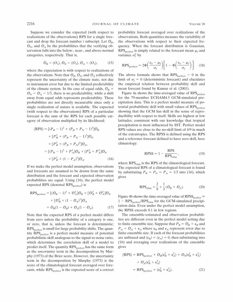
Figure 4a shows the time-averaged value of RPSperfect

for the 79-member ECHAM4.5 GCM-simulated pre-cipitation data. This is a perfect model measure of po-tential probabilistic skill with small values of RPSperfect

showing that the GCM has skill in the sense of repro-ducibility with respect to itself. Skills are highest at lowlatitudes, consistent with our knowledge that tropicalprecipitation is most influenced by SST. Perfect modelRPS values are close to the no-skill limit of 4/9 in muchof the extratropics. The RPSS is defined using the RPSand a reference forecast defined to have zero skill, hereclimatology:

RPSS � 1 �RPS

RPSclim, �19�

where RPSclim is the RPS of the climatological forecast.The expected RPS of a climatological forecast is foundby substituting PB � PN � PA � 1/3 into (16), whichgives

RPSclim �29

�13

�OB � OA�. �20�

Figure 4b shows the time-averaged value of RPSSperfect �1 � RPSperfect/RPSclim for the GCM-simulated precipi-tation data. Even under the perfect model assumption,the RPSS exceeds 0.1 in few regions.

The ensemble-estimated and observation probabili-ties are different even in the perfect model setting dueto finite ensemble size. Suppose that PB � OB � �B andPA � OA � �A where �B and �A represent error due tofinite ensemble size. If each of the forecast probabilitiesare unbiased and ��B� � ��A� � 0, then substituting into(16) and averaging over realizations of the ensemblegives

�RPS� � RPSperfect � OB��B2 � �A

2 � � ON��B2 � �A

2 �

� OA��B2 � �A

2 �

� RPSperfect � ��B2 � �A

2 �. �21�


This means that the perfect model expected RPS isincreased by an amount that depends on the variance ofthe probability estimate. In particular, if the samplingerror is associated with the counting estimate whosevariance is given by (3), then

��B2 � �A

2 � �1N

�OB�1 � OB� � OA�1 � OA��

�22�

and

�RPS� � �1 �1N�RPSperfect. �23�

It follows that

�RPSS� � 1 � �1 �1N� RPSperfect

RPSclim,

��N � 1�RPSSperfect � 1

N. �24�

The relation between RPSS and ensemble size is thesame as that for the Brier skill score (Richardson 2001).The relation in (24) quantifies the degradation of RPSSdue to sampling error and, combined with (18), pro-vides an analytical expression for the empirical relation

between ensemble size, RPSS, and mean forecast foundin Kumar et al. (2001).

If the tercile probability estimate has variance thatdiffers from that of the counting estimate by some fac-tor �, as does, for example, the Gaussian fit estimate,then

RPSS ��N � �RPSSperfect �

N, �25�

where degradation of the RPSS is reduced for � � 1.

4. Estimates of GCM-simulated seasonalprecipitation tercile probability


The average variance of the counting estimate in (5)was derived assuming Gaussian distributions. To seehow well this approximation describes the behavior ofGCM-simulated December–February precipitation to-tals, we compare the average counting estimate vari-ance in (5) to that computed by subsampling from the79-member ensemble of GCM simulations. We use thefact that the average squared difference of two inde-pendent counting estimates is twice the variance. Morespecifically, we select two independent samples of size

FIG. 4. Perfect model measures of potential probability forecast skill (a) RPSperfect and (b)RPSSperfect for DJF precipitation.

15 MAY 2007 T I P P E T T E T A L . 2217

Fig 4 live 4/C

N (without replacement) from the ensemble of GCMsimulations and compute two counting estimate prob-abilities denoted pN and p�N; the ensemble size of 79 andindependence requirement limits the maximum valueof N to 39. The expected value of the square of thedifference between the two counting estimates pN andp�N is twice the variance of the counting estimate since

��pN � pN�2� � ��pN � p� � �pN � pN��2�

� 2��pN � p�2�, �26�

where we use the fact that the sampling errors (pN � p)and (p � p�N) are uncorrelated. The averages in (26) arewith respect to time and realizations (1000) of the twoindependent samples.

We expect especially close agreement between thesubsampling calculations and the analytical results of(5) in regions where there is little predictability and thesignal-to-noise ratio S2 is small, since, for S2 � 0, theanalytical result is exact. In regions where the signal-to-noise ratio is not zero, though generally fairly small,we expect that the average counting variance still de-creases as 1/N. However, there is no guarantee that theGaussian approximation will provide an adequate de-scription of the actual behavior of the GCM data.

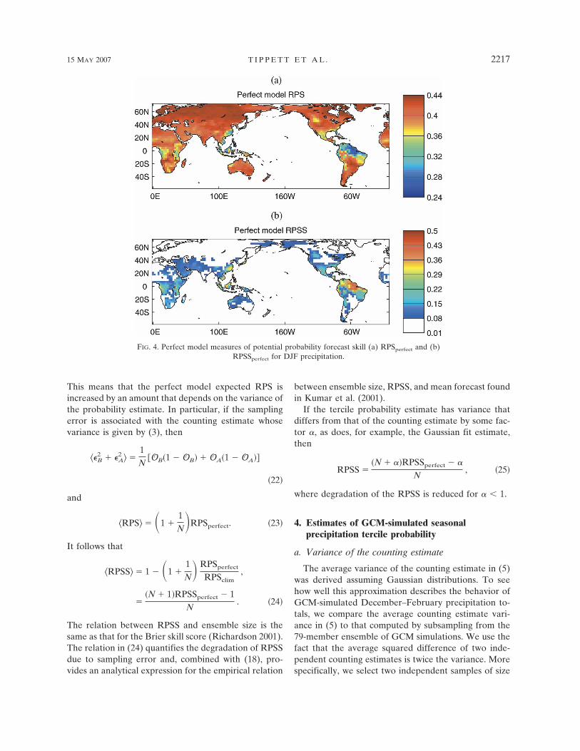
Figure 5 shows that in the land gridpoint average thevariance of the counting estimate is very well describedby the analytical result in (5), with the difference fromthe analytical result being on the order of a few percentfor the below-normal category probability and less thanone percent for the above-normal category probability.The accuracy difference between the below- and above-normal categories may be due to the below-normal cat-egory being more affected by non-Gaussian behavior.

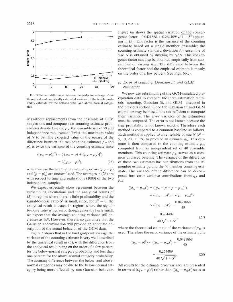
Figure 6a shows the spatial variation of the conver-gence factor �0.0421868 � 0.264409/�1 � S2 appear-ing in (5). This factor is the variance of the countingestimate based on a single member ensemble; thecounting estimate standard deviation for ensemble ofsize N is obtained by dividing by �N. This conver-gence factor can also be obtained empirically from sub-samples of varying size. The difference between thetheoretical factor and the empirical estimate is mostlyon the order of a few percent (see Figs. 6b,c).

b. Error of counting, Gaussian fit, and GLMestimators

We now use subsampling of the GCM-simulated pre-cipitation data to compare the three estimation meth-ods—counting, Gaussian fit, and GLM—discussed inthe previous section. Since the Gaussian fit and GLMestimators may be biased, it is not sufficient to computetheir variance. The error variance of the estimatorsmust be computed. The error is not known because thetrue probability is not known exactly. Therefore eachmethod is compared to a common baseline as follows.Each method is applied to an ensemble of size N (N �5, 10, 20, 30, 39) to produce an estimate qN. This esti-mate is then compared to the counting estimate p40

computed from an independent set of 40 ensemblemembers. This counting estimate p40 serves as a com-mon unbiased baseline. The variance of the differenceof these two estimates has contributions from the N-member estimate qN and the 40-member counting esti-mate. The variance of the difference can be decom-posed into error variance contributions from qN andp40:

��qN � p40�2� � ��qN � p � p � p40�2�

� ��qN � p�2� � �� p � p40�2�

� ��qN � p�2� �0.0421868

40

�0.264409

40�1 � S2, �27�

where the theoretical estimate of the variance of p40 isused. Therefore the error variance of the estimate qN is

��qN � p�2� � ��qN � p40�2� �0.0421868

40

�0.264409

40�1 � S2. �28�

All results for the estimate error variance are presentedin terms of �(qN � p)2� rather than �(qN � p40)2� so as to

FIG. 5. Percent difference between the gridpoint average of thetheoretical and empirically estimated variance of the tercile prob-ability estimate for the below-normal and above-normal catego-ries.


give a sense of the magnitude of the sampling errorrather than the difference with the baseline estimate.Results are averaged over time and realizations (100) ofthe N-member estimate and the 40-member countingestimate.

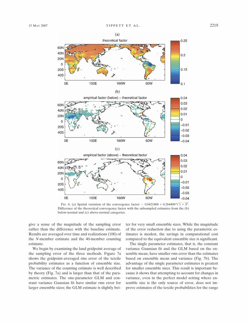
We begin by examining the land gridpoint average ofthe sampling error of the three methods. Figure 7ashows the gridpoint-averaged rms error of the tercileprobability estimates as a function of ensemble size.The variance of the counting estimate is well describedby theory (Fig. 7a) and is larger than that of the para-metric estimates. The one-parameter GLM and con-stant variance Gaussian fit have similar rms error forlarger ensemble sizes; the GLM estimate is slightly bet-

ter for very small ensemble sizes. While the magnitudeof the error reduction due to using the parametric es-timates is modest, the savings in computational costcompared to the equivalent ensemble size is significant.

The single parameter estimates, that is, the constantvariance Gaussian fit and the GLM based on the en-semble mean, have smaller rms error than the estimatesbased on ensemble mean and variance (Fig. 7b). Theadvantage of the single parameter estimates is greatestfor smaller ensemble sizes. This result is important be-cause it shows that attempting to account for changes invariance, even in the perfect model setting where en-semble size is the only source of error, does not im-prove estimates of the tercile probabilities for the range

FIG. 6. (a) Spatial variation of the convergence factor � 0.0421868 � 0.264409/�1 � S2.Difference of the theoretical convergence factor with the subsampled estimates from the (b)below-normal and (c) above-normal categories.

15 MAY 2007 T I P P E T T E T A L . 2219

Fig 6 live 4/C

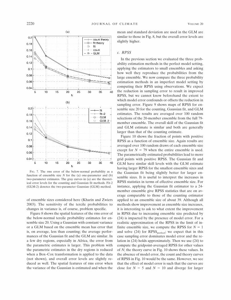
of ensemble sizes considered here (Kharin and Zwiers2003). The sensitivity of the tercile probabilities tochanges in variance is, of course, problem specific.

Figure 8 shows the spatial features of the rms error ofthe below-normal tercile probability estimates for en-semble size 20. Using a Gaussian with constant varianceor a GLM based on the ensemble mean has error thatis, on average, less than counting; the average perfor-mances of the Gaussian fit and the GLM are similar. Ina few dry regions, especially in Africa, the error fromthe parametric estimates is larger. This problem withthe parametric estimates in the dry regions is reducedwhen a Box–Cox transformation is applied to the data(not shown), and overall error levels are slightly re-duced as well. The spatial features of rms error whenthe variance of the Gaussian is estimated and when the

mean and standard deviation are used in the GLM aresimilar to those in Fig. 8, but the overall error levels areslightly higher.

c. RPSS

In the previous section we evaluated the three prob-ability estimation methods in the perfect model setting,applying the estimators to small ensembles and askinghow well they reproduce the probabilities from thelarge ensemble. We now compare the three probabilityestimation methods in an imperfect model setting bycomputing their RPSS using observations. We expectthe reduction in sampling error to result in improvedRPSS, but we cannot know beforehand the extent towhich model error confounds or offsets the reduction insampling error. Figure 9 shows maps of RPSS for en-semble size 20 for the counting, Gaussian fit, and GLMestimates. The results are averaged over 100 randomselections of the 20-member ensemble from the full 79-member ensemble. The overall skill of the Gaussian fitand GLM estimate is similar and both are generallylarger than that of the counting estimate.

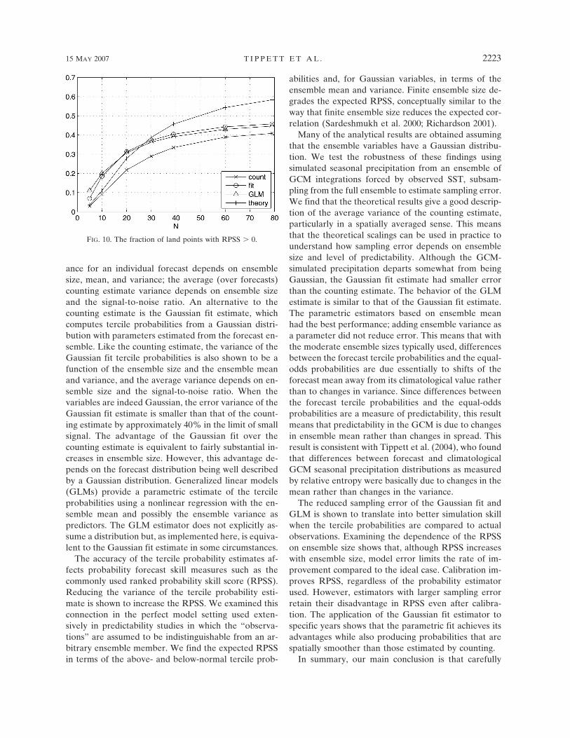
Figure 10 shows the fraction of points with positiveRPSS as a function of ensemble size. Again results areaveraged over 100 random draws of each ensemble sizeexcept for N � 79 when the entire ensemble is used.The parametrically estimated probabilities lead to moregrid points with positive RPSS. The Gaussian fit andGLM have similar skill levels with the GLM estimatehaving larger RPSS for the smallest ensemble sizes andthe Gaussian fit being slightly better for larger en-semble sizes. It is useful to interpret the increases inRPSS statistics in terms of effective ensemble size. Forinstance, applying the Gaussian fit estimator to a 24-member ensemble give RPSS statistics that are on av-erage comparable to those of the counting estimatorapplied to an ensemble size of about 39. Although allmethods show improvement as ensemble size increases,it is interesting to ask to what extent the improvementin RPSS due to increasing ensemble size predicted by(24) is impacted by the presence of model error. For arealistic approximation of the RPSS in the limit of in-finite ensemble size, we compute the RPSS for N � 1and solve (24) for RPSSperfect; we expect that in thiscase sampling error dominates model error and the re-lation in (24) holds approximately. Then we use (24) tocompute the gridpoint-averaged RPSS for other valuesof N; the theory curve in Fig. 10 shows these values. Inthe absence of model error, the count and theory curvesof RPSS in Fig. 10 would be the same. However, we seethat the effect of model error is such that the curves areclose for N � 5 and N � 10 and diverge for larger

FIG. 7. The rms error of the below-normal probability as afunction of ensemble size N for the (a) one-parameter and (b)two-parameter estimates. The gray curves in (a) are the theoret-ical error levels for the counting and Gaussian fit methods. Fit-2(GLM-2) denotes the two-parameter Gaussian (GLM) method.


ensemble sizes with the actual increase in RPSS beinglower than that predicted by (24).

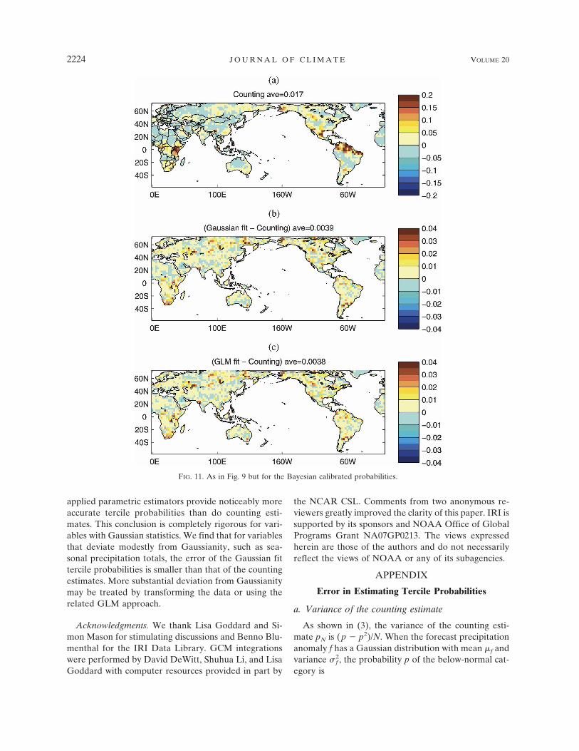
The presence of model error means that some cali-bration of the model output with observations isneeded. The GCM ensemble tends to be overconfidentand calibration tempers this. To see if reducing sam-pling error still has a noticeable impact after calibra-tion, we use a simple version of Bayesian weighting(Rajagopalan et al. 2002; Robertson et al. 2004). In themethod, the calibrated probability is a weighted aver-age of the GCM probability and the climatology prob-ability (1/3). The weights are chosen to maximize thelikelihood of the observations. There is cross-validation

in the sense that the weights are computed with a par-ticular ensemble of size N, and the RPSS is computedby applying those weights to a different ensemble of thesame size and then comparing the result with observa-tions. The calibrated counting–estimated probabilitiesstill have slightly negative RPSS in some areas (Fig.11a), but the overall amount of positive RPSS is in-creased compared to the uncalibrated simulations (cf.with Fig. 9a); the ensemble size is 20 and results areaveraged over 100 realizations. The calibrated Gauss-ian and GLM probabilities have modestly higher over-all RPSS than the calibrated counting estimates withnoticeable improvement in skillful areas like southern

FIG. 8. (a) The rms error of the counting estimate of the below-normal tercile probabilitywith ensemble size 20. The rms error of the counting error minus that of the (b) Gaussian fitand (c) the GLM based on the ensemble mean. The gridpoint averages are shown in the titles.

15 MAY 2007 T I P P E T T E T A L . 2221

Fig 8 live 4/C

Africa (Figs. 11b,c). We note that a simpler calibrationmethod based on a Gaussian fit with the variance de-termined by the correlation between ensemble meanand observations, as in Tippett et al. (2005), ratherthan ensemble spread, performs nearly as well as theGaussian fit with Bayesian calibration.

It is interesting to look at examples of the probabili-ties given by the counting and Gaussian fit estimate tosee how the spatial distributions of probabilities maydiffer in appearance. Figure 12 shows uncalibrated ter-cile probabilities from DJF 1996 (ENSO neutral) and1998 (strong El Niño). Counting and Gaussian prob-abilities appear similar, with Gaussian probabilities ap-pearing spatially smoother.

5. Summary and conclusions

Here we have explored how the accuracy of tercilecategory probability estimates are related to ensemblesize and the chosen probability estimation technique.The counting estimate, which uses the fraction of en-semble members that fall in the tercile category, is at-tractive because it is simple and places no restrictionson the form of the ensemble distribution. The errorvariance of the counting estimate is a function of theensemble size and tercile category probability. ForGaussian variables, the tercile category probability is afunction of the ensemble mean and variance. There-fore, for Gaussian variables, the counting estimate vari-

FIG. 9. RPSS of (a) the counting-based probabilities and its difference with that of the (b)Gaussian and (c) GLM-estimated probabilities. Positive values in (b) and (c) correspond toincreased RPSS compared to counting. The gridpoint averages are shown in the titles.


Fig 9 live 4/C

ance for an individual forecast depends on ensemblesize, mean, and variance; the average (over forecasts)counting estimate variance depends on ensemble sizeand the signal-to-noise ratio. An alternative to thecounting estimate is the Gaussian fit estimate, whichcomputes tercile probabilities from a Gaussian distri-bution with parameters estimated from the forecast en-semble. Like the counting estimate, the variance of theGaussian fit tercile probabilities is also shown to be afunction of the ensemble size and the ensemble meanand variance, and the average variance depends on en-semble size and the signal-to-noise ratio. When thevariables are indeed Gaussian, the error variance of theGaussian fit estimate is smaller than that of the count-ing estimate by approximately 40% in the limit of smallsignal. The advantage of the Gaussian fit over thecounting estimate is equivalent to fairly substantial in-creases in ensemble size. However, this advantage de-pends on the forecast distribution being well describedby a Gaussian distribution. Generalized linear models(GLMs) provide a parametric estimate of the tercileprobabilities using a nonlinear regression with the en-semble mean and possibly the ensemble variance aspredictors. The GLM estimator does not explicitly as-sume a distribution but, as implemented here, is equiva-lent to the Gaussian fit estimate in some circumstances.

The accuracy of the tercile probability estimates af-fects probability forecast skill measures such as thecommonly used ranked probability skill score (RPSS).Reducing the variance of the tercile probability esti-mate is shown to increase the RPSS. We examined thisconnection in the perfect model setting used exten-sively in predictability studies in which the “observa-tions” are assumed to be indistinguishable from an ar-bitrary ensemble member. We find the expected RPSSin terms of the above- and below-normal tercile prob-

abilities and, for Gaussian variables, in terms of theensemble mean and variance. Finite ensemble size de-grades the expected RPSS, conceptually similar to theway that finite ensemble size reduces the expected cor-relation (Sardeshmukh et al. 2000; Richardson 2001).

Many of the analytical results are obtained assumingthat the ensemble variables have a Gaussian distribu-tion. We test the robustness of these findings usingsimulated seasonal precipitation from an ensemble ofGCM integrations forced by observed SST, subsam-pling from the full ensemble to estimate sampling error.We find that the theoretical results give a good descrip-tion of the average variance of the counting estimate,particularly in a spatially averaged sense. This meansthat the theoretical scalings can be used in practice tounderstand how sampling error depends on ensemblesize and level of predictability. Although the GCM-simulated precipitation departs somewhat from beingGaussian, the Gaussian fit estimate had smaller errorthan the counting estimate. The behavior of the GLMestimate is similar to that of the Gaussian fit estimate.The parametric estimators based on ensemble meanhad the best performance; adding ensemble variance asa parameter did not reduce error. This means that withthe moderate ensemble sizes typically used, differencesbetween the forecast tercile probabilities and the equal-odds probabilities are due essentially to shifts of theforecast mean away from its climatological value ratherthan to changes in variance. Since differences betweenthe forecast tercile probabilities and the equal-oddsprobabilities are a measure of predictability, this resultmeans that predictability in the GCM is due to changesin ensemble mean rather than changes in spread. Thisresult is consistent with Tippett et al. (2004), who foundthat differences between forecast and climatologicalGCM seasonal precipitation distributions as measuredby relative entropy were basically due to changes in themean rather than changes in the variance.

The reduced sampling error of the Gaussian fit andGLM is shown to translate into better simulation skillwhen the tercile probabilities are compared to actualobservations. Examining the dependence of the RPSSon ensemble size shows that, although RPSS increaseswith ensemble size, model error limits the rate of im-provement compared to the ideal case. Calibration im-proves RPSS, regardless of the probability estimatorused. However, estimators with larger sampling errorretain their disadvantage in RPSS even after calibra-tion. The application of the Gaussian fit estimator tospecific years shows that the parametric fit achieves itsadvantages while also producing probabilities that arespatially smoother than those estimated by counting.

In summary, our main conclusion is that carefully

FIG. 10. The fraction of land points with RPSS � 0.

15 MAY 2007 T I P P E T T E T A L . 2223

applied parametric estimators provide noticeably moreaccurate tercile probabilities than do counting esti-mates. This conclusion is completely rigorous for vari-ables with Gaussian statistics. We find that for variablesthat deviate modestly from Gaussianity, such as sea-sonal precipitation totals, the error of the Gaussian fittercile probabilities is smaller than that of the countingestimates. More substantial deviation from Gaussianitymay be treated by transforming the data or using therelated GLM approach.

Acknowledgments. We thank Lisa Goddard and Si-mon Mason for stimulating discussions and Benno Blu-menthal for the IRI Data Library. GCM integrationswere performed by David DeWitt, Shuhua Li, and LisaGoddard with computer resources provided in part by

the NCAR CSL. Comments from two anonymous re-viewers greatly improved the clarity of this paper. IRI issupported by its sponsors and NOAA Office of GlobalPrograms Grant NA07GP0213. The views expressedherein are those of the authors and do not necessarilyreflect the views of NOAA or any of its subagencies.

APPENDIX

Error in Estimating Tercile Probabilities


As shown in (3), the variance of the counting esti-mate pN is (p � p2)/N. When the forecast precipitationanomaly f has a Gaussian distribution with mean �f andvariance 2

f , the probability p of the below-normal cat-egory is

FIG. 11. As in Fig. 9 but for the Bayesian calibrated probabilities.


Fig 11 live 4/C

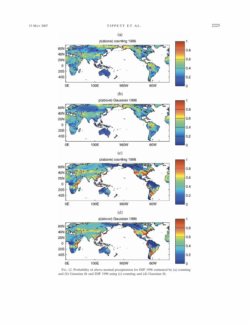
FIG. 12. Probability of above-normal precipitation for DJF 1996 estimated by (a) countingand (b) Gaussian fit and DJF 1998 using (c) counting and (d) Gaussian fit.

15 MAY 2007 T I P P E T T E T A L . 2225

Fig 12 live 4/C

p � probability{ f � xb} �1

�2��f

��

xb

exp��f � �f�

2

2� f2 � df � ��xb � �f

�f� �

12 �1 � erf�xb � �f

�2�f��,

�A1�

where � is the normal cumulative distribution function,erf denotes the error function, and xb is the left tercileboundary of the climatological distribution. In this case,the counting estimate variance depends on the forecastmean and variance through

1N

�p � p2� �1

4N�1 � �erf�xb � �f

�2�f��2�.

�A2�

Similar relations hold for the above-normal category.Suppose that the precipitation anomaly x is joint nor-

mally distributed with mean zero and variance 2x. In

this paper, the forecast f is the precipitation anomaly xconditioned on the SST. In this case, the left tercileboundary xb of the climatological pdf is xx0, wherex0 � ��1(1/3) � �0.4307 is the left tercile boundary of

a mean zero normal distribution with unit variance. Av-eraging x2 over all forecasts gives

�x2� � �x2 � ��f

2� � � f2, �A3�

which decomposes the climatological variance 2x into

signal and noise contributions. We denote the signalvariance ��2

f � by 2s and define the signal-to-noise ratio

by

S2 �� s

2

� f2 . �A4�

Equation (A2) gives the counting estimate variance fora particular forecast. The average counting estimatevariance is found by taking the average of (A2) withrespect to forecasts. Since the forecast mean is Gauss-ian with mean zero and variance 2

s � 2f S2,

�p � p2� �1

�2��s

��

� 14�1 � �erf�xb � �f

�2�f��2� exp��

� �f2

2� s2 � d�f . �A5�

To show that the average counting estimate variance is a function of only the signal-to-noise ratio S2, weintroduce the variable � � �f / f and use the fact that xb/ f � x0�1 � S2, to obtain

�p � p2� �1

�2�S�

��

� 14�1 ��erf�x0�1 � S2 � �

�2��2� exp��

�2

2S2� d� . �A6�

Equation (A6) gives �p � p2� as a function of the signal-to-noise ratio S2. Numerical evaluation of the integralin (A6) suggests that we express this dependence using a new parameter g � (1 � S2)�1/2:

�p � p2� �g

4�2��g2 � 1�

��

� �1 � �erf�x0 g � �

�2��2� exp��

g2�2

2�g2 � 1�� d� . �A7�

To approximate the dependence of the average vari-ance on the signal-to-noise ratio, we perform a seriesexpansion about g � 1 corresponding to the signal-to-noise ratio S2 being zero. The first term is found from

�p � p2�g�1 �29

, �A8�

and then numerical computation gives that

d

dg �p � p2�g�1 � 0.264409. �A9�

An approximation of �p � p2� is

�p � p2� �29

� 0.264409�g � 1� � O�g � 1�2 �A10�

or in terms of the signal-to-noise ratio


�p � p2�N

� �0.0421868

N�

0.264409

N�1 � S2. �A11�

This approximation is valid for small values of S2. Asecond-order [in powers of (g � 1)] approximation ismore accurate for larger values of S and is given by

�p � p2�N

�0.0393036

N�

0.101429

N�1 � S2�

0.0814898

N�1 � S2�.

�A12�

Since S2 is fairly small for seasonal forecasts, we will usethe approximation in (A11).

b. Error of the Gaussian fit estimate

Suppose the distributions are indeed Gaussian. Wefit the N-member forecast ensemble with a Gaussiandistribution, using its sample mean mf and sample vari-ance s2

f defined by

mf �1N

i�1

N

xi,

sf2 �

1N � 1

i�1

N

�xi � mf�2, �A13�

where xi denotes the value of the ith member of theensemble. Based on this information and using (A1),the Gaussian fit estimate gN of the probability of thebelow-normal category is

gN � ��xb � mf

sf� �

12 �1 � erf�xb � mf

�2sf��. �A14�

The squared error of the Gaussian fit probability esti-mate is

�gN � p�2 � �12 �1 � erf�xb � mf

�2sf��

�12 �1 � erf�xb � �f

�2�f��2

.

�A.15�

The error of the Gaussian fit probability estimate is dueto the difference between the population values and thesample estimates of the forecast mean and variance.

If there is no predictability and the signal-to-ratio iszero, then the forecast mean �f is zero and the truetercile probability is 1/3 for all forecasts. Also, the fore-cast variance 2

f is equal to the climatological variance 2

x and does not have to be estimated from the en-semble. In this case, the squared error of the Gaussianfit estimate is

�13

�12 �1 � erf�xb � mf

�2�x��2

�mf

2e�x02

2��x2 � O�mf

3�,

�A16�

where we have made a Maclaurin expansion in mf andused the fact that xb � xx0. The term O(m3

f ) is smalland can be neglected for sufficiently large ensemblesize N; neglecting the higher-order terms leads to anunderestimate in the final result of about 3.6% for N �10. Since �m2

f � � 2x /N, the average (over forecasts) vari-

ance of the Gaussian fit tercile probability is

�mf2e�x0

2

2��x2 �

e�x02

2�N�

0.1322N

. �A17�

On the other hand, suppose that the forecast mean isnot identically zero, but the forecast variance f is con-stant and known. This means that there is predictabilitydue to changes in forecast mean but not due to changesin forecast variance. The squared error of the Gaussianfit probability estimate is

�gN � p�2 � �12 �1 � erf�xb � mf

�2�f��

�12 �1 � erf�xb � �f

�2�f��2

. �A18�

The error of the Gaussian fit probability is due entirelyto the error in estimating the mean. Expanding thisexpression in a Taylor series in powers of (mf � �f)about mf � �f gives that the squared error is

�gN � p�2 ��mf � �f�

2

2�� f2 exp��xb � �f

�f�2�

� O��f � mf�3. �A19�

We now take the expectation of the leading order termin (A19) with respect to realizations of the ensemble.Since the variance of the sample mean is �(�f � mf)

2� � 2

f /N, the average (over realizations of the ensemble) ofthe squared error of the Gaussian fit is

�gN � p�2 �1

2�Nexp��xb � �f

�f�2�. �A20�

Equation (A20) gives the squared error of the Gaussianfit tercile probability for a particular forecast. Averag-ing (A20) over mean forecasts �f with mean zero andvariance 2

s gives that the average variance of theGaussian fit tercile probability is

15 MAY 2007 T I P P E T T E T A L . 2227

��gN � p�2� �1

�2��3 2�sN�

��

�

exp��xb � �f

�f�2� exp��

�f2

2� s2� d� f �

exp��1 � S2

1 � 2S2 x02�

2�N�1 � 2S2, �A21�

where we use the relation x2b / 2

f � x20(1 � S2).

REFERENCES

Atger, F., 1999: The skill of ensemble prediction systems. Mon.Wea. Rev., 127, 1941–1953.

Barnston, A. G., S. J. Mason, L. Goddard, D. G. Dewitt, and S. E.Zebiak, 2003: Multimodel ensembling in seasonal climateforecasting at IRI. Bull. Amer. Meteor. Soc., 84, 1783–1796.

Buizza, R., and T. N. Palmer, 1998: Impact of ensemble size onensemble prediction. Mon. Wea. Rev., 126, 2503–2518.

DelSole, T., 2004: Predictability and information theory. Part I:Measures of predictability. J. Atmos. Sci., 61, 2425–2440.

——, and M. K. Tippett, 2007: Predictability, information theory,and stochastic models. Rev. Geophys., in press.

Epstein, E. S., 1969: A scoring system for probability forecasts ofranked categories. J. Appl. Meteor., 8, 985–987.

Hamill, T. M., J. S. Whitaker, and X. Wei, 2004: Ensemble refor-ecasting: Improving medium-range forecast skill using retro-spective forecasts. Mon. Wea. Rev., 132, 1434–1447.

Kharin, V. V., and F. W. Zwiers, 2003: Improved seasonal prob-ability forecasts. J. Climate, 16, 1684–1701.

Kleeman, R., 2002: Measuring dynamical prediction utility usingrelative entropy. J. Atmos. Sci., 59, 2057–2072.

——, and A. M. Moore, 1999: A new method for determining thereliability of dynamical ENSO predictions. Mon. Wea. Rev.,127, 694–705.

Kumar, A., A. G. Barnston, and M. P. Hoerling, 2001: Seasonalpredictions, probabilistic verifications, and ensemble size. J.Climate, 14, 1671–1676.

McCullagh, P., and J. A. Nelder, 1989: Generalized Linear Mod-els. Chapman and Hall, 387 pp.

Murphy, A. H., 1973: A new vector partition of the probabilityscore. J. Appl. Meteor., 12, 595–600.

New, M., M. Hulme, and P. Jones, 2000: Representing twentieth-century space–time climate variability. Part II: Developmentof 1901–96 monthly grids of terrestrial surface climate. J. Cli-mate, 13, 2217–2238.

Rajagopalan, B., U. Lall, and S. E. Zebiak, 2002: Categorical cli-mate forecasts through regularization and optimal combina-tion of multiple GCM ensembles. Mon. Wea. Rev., 130, 1792–1811.

Richardson, D. S., 2001: Measures of skill and value of ensembleprediction systems, their interrelationship and the effect ofensemble size. Quart. J. Roy. Meteor. Soc., 127, 2473–2489.

Robertson, A. W., U. Lall, S. E. Zebiak, and L. Goddard, 2004:Improved combination of multiple atmospheric GCM en-sembles for seasonal prediction. Mon. Wea. Rev., 132, 2732–2744.

Roeckner, E., and Coauthors, 1996: The atmospheric general cir-culation model ECHAM-4: Model description and simula-tion of present-day climate. Max Planck Institute for Meteo-rology Tech. Rep. 218, 90 pp.

Sardeshmukh, P. D., G. P. Compo, and C. Penland, 2000: Changesof probability associated with El Niño. J. Climate, 13, 4268–4286.

Tippett, M. K., R. Kleeman, and Y. Tang, 2004: Measuring thepotential utility of seasonal climate predictions. Geophys.Res. Lett., 31, L22201, doi:10.1029/2004GL021575.

——, L. Goddard, and A. G. Barnston, 2005: Statistical–dynam-ical seasonal forecasts of central-southwest Asian winter pre-cipitation. J. Climate, 18, 1831–1843.

Wilks, D. S., 2002: Smoothing forecast ensembles with fitted prob-ability distributions. Quart. J. Roy. Meteor. Soc., 128, 2821–2836.


estimation of seasonal precipitation tercile-based

Documents