estimation of multiple-regime threshold autoregressive models with structural breaks
TRANSCRIPT

This article was downloaded by: [Kungliga Tekniska Hogskola]On: 11 October 2014, At: 11:29Publisher: Taylor & FrancisInforma Ltd Registered in England and Wales Registered Number: 1072954 Registered office: Mortimer House,37-41 Mortimer Street, London W1T 3JH, UK
Journal of the American Statistical AssociationPublication details, including instructions for authors and subscription information:http://amstat.tandfonline.com/loi/uasa20
Estimation of Multiple-Regime ThresholdAutoregressive Models with Structural BreaksChun Yip Yaua, Chong Man Tanga & Thomas C. M. Leeb
a Chinese University of Hong Kongb University of California at DavisAccepted author version posted online: 25 Sep 2014.
To cite this article: Chun Yip Yau, Chong Man Tang & Thomas C. M. Lee (2014): Estimation of Multiple-RegimeThreshold Autoregressive Models with Structural Breaks, Journal of the American Statistical Association, DOI:10.1080/01621459.2014.954706
To link to this article: http://dx.doi.org/10.1080/01621459.2014.954706
Disclaimer: This is a version of an unedited manuscript that has been accepted for publication. As a serviceto authors and researchers we are providing this version of the accepted manuscript (AM). Copyediting,typesetting, and review of the resulting proof will be undertaken on this manuscript before final publication ofthe Version of Record (VoR). During production and pre-press, errors may be discovered which could affect thecontent, and all legal disclaimers that apply to the journal relate to this version also.
PLEASE SCROLL DOWN FOR ARTICLE
Taylor & Francis makes every effort to ensure the accuracy of all the information (the “Content”) containedin the publications on our platform. However, Taylor & Francis, our agents, and our licensors make norepresentations or warranties whatsoever as to the accuracy, completeness, or suitability for any purpose of theContent. Any opinions and views expressed in this publication are the opinions and views of the authors, andare not the views of or endorsed by Taylor & Francis. The accuracy of the Content should not be relied upon andshould be independently verified with primary sources of information. Taylor and Francis shall not be liable forany losses, actions, claims, proceedings, demands, costs, expenses, damages, and other liabilities whatsoeveror howsoever caused arising directly or indirectly in connection with, in relation to or arising out of the use ofthe Content.
This article may be used for research, teaching, and private study purposes. Any substantial or systematicreproduction, redistribution, reselling, loan, sub-licensing, systematic supply, or distribution in anyform to anyone is expressly forbidden. Terms & Conditions of access and use can be found at http://amstat.tandfonline.com/page/terms-and-conditions
ACCEPTED MANUSCRIPT
Estimation of Multiple-Regime ThresholdAutoregressive Models with Structural Breaks
Chun Yip Yau∗
Chinese University of Hong KongChong Man Tang†
Chinese University of Hong Kong
Thomas C. M. Lee‡
University of California at Davis
Abstract
The threshold autoregressive (TAR) model is a class of nonlinear time series models that
have been widely used in many areas. Due to its nonlinear nature, one major difficulty in fitting
a TAR model is the estimation of the thresholds. As a first contribution, this paper develops an
automatic procedure to estimate the number and values of the thresholds, as well as the corre-
sponding AR order and parameter values in each regime. These parameter estimates are defined
as the minimizers of an objective function derived from the minimum description length (MDL)
principle. A genetic algorithm is constructed to efficiently solve the associated minimization
problem. The second contribution of this paper is the extension of this framework to piecewise
TAR modeling; i.e., the time series is partitioned into different segments for which each seg-
ment can be adequately modeled by a TAR model, while models from adjacent segments are
different. For such piecewise TAR modeling, a procedure is developed to estimate the number
and locations of the breakpoints, together with all other parameters in each segment. Desirable
theoretical results are derived to lend support to the proposed methodology. Simulation experi-
ments and an application to an U.S. GNP data are used to illustrate the empirical performances
of the methodology.
∗Department of Statistics, Chinese University of Hong Kong, Shatin, N.T., Hong Kong. Email:[email protected]. Supported in part by HKSAR-RGC Grants CUHK405012, 405113 and Direct GrantCUHK2060445.
†Department of Statistics, Chinese University of Hong Kong, Shatin, N.T., Hong Kong. Email:[email protected]
‡Department of Statistics, University of California at Davis, Davis, CA 95616, USA. Email:[email protected]. Supported in part by the National Science Foundation under Grants 1007520, 1209226 and1209232.
1ACCEPTED MANUSCRIPT
Dow
nloa
ded
by [
Kun
glig
a T
ekni
ska
Hog
skol
a] a
t 11:
29 1
1 O
ctob
er 2
014

ACCEPTED MANUSCRIPT
Keywords: change-point detection, genetic algorithms, minimum description length principle,
multiple-threshold, nonstationary time series, piecewise modeling
1 Introduction
The (r + 1)-regime threshold autoregressive (TAR) model, defined by
Xt =
r+1∑
j=1
(Φ′jX
( j)t−1 + σ jet
)I (θ j−1 < Xt−d ≤ θ j) , et ∼ IID(0,1), (1)
whereX( j)t−1 = (1,Xt−1, . . . ,Xt−pj ), asserts that the autoregressive structure of the process{Xt} is
governed by the range of values ofXt−d. The integer-valued quantityd is known as the delay
parameter and the parameters−∞ = θ0 < θ1 < ∙ ∙ ∙ < θr < θr+1 = ∞ are called the thresholds.
These thresholds partition the space ofXt−d into r + 1 regimes, in which thej-th regime follows an
AR model with with orderpj, coefficient parameterΦ j and white noise varianceσ2j . Since its initial
proposal by Tong (1978), the TAR model has attracted enormous attention from the nonlinear time
series literature. It has also been applied to study real data behaviors in many areas, especially
econometrics and finance. Excellent surveys on the TAR models can be found in Tong (1990,
2011).
For parameter estimation, Chan (1993) considers the least square estimation for a two-regime
TAR model and established its large sample theory. Li and Ling (2012) extend the theory to a
multiple-regime TAR models. In particular, it is shown that, when the number of thresholds is
known, each estimated threshold is√
n-consistent and converges weakly to the smallest minimizer
of a two-sided compound Poisson process. Also, the estimated thresholds are asymptotically in-
dependent. Moreover, if the AR order is known, the AR parameter estimates in each regime are√
n-consistent and asymptotically normal.
Despite the well developed theoretical background of the estimation theory, the estimation
procedure of TAR models demands a high computational cost due to the irregular nature of the
threshold parameters; e.g., see Li and Ling (2012). In particular, for a (r + 1)-regime TAR model,
2ACCEPTED MANUSCRIPT
Dow
nloa
ded
by [
Kun
glig
a T
ekni
ska
Hog
skol
a] a
t 11:
29 1
1 O
ctob
er 2
014

ACCEPTED MANUSCRIPT
locating the global minimum of the least squares criterion requires a multi-parameter grid search
over all possible values of ther threshold parameters, which is typically computational infeasible.
In order to circumvent this difficulty, Tsay (1989) transforms (1) into a change-point model and
proposes a graphical approach to help visually determine the number and values of the thresholds.
Coakleyet al.(2003) use similar techniques to develop an estimation approach that is based on QR
factorizations of matrices. When the number of thresholdsr is unknown, Gonzalo and Pitarakis
(2002) suggest a sequential estimation procedure for choosingr, under the assumption that all
σ js are equal. We are not aware of any results for more general models. In particular, when the
number of thresholds and the order of the AR model in each regime are unknown and theσ js are
not assumed equal, no practical estimation method appears available.
In this paper, motivated by the close connection between TAR model and the structural break
model suggested by Tsay (1989), we propose an automatic procedure to estimate the number and
values of thresholds, as well as to perform model selection in each regime. The procedure is based
on an objective function derived from the minimum description length (MDL) principle, for which
the best fitting TAR model is defined as its minimizer. A genetic algorithm is developed to provide
an efficient computational method for corresponding minimization problem. We shall establish
the consistency of our MDL estimates for the number and locations of the thresholds, the delay
parameter and the AR orders in each regime. Moreover, the convergence rate of the thresholds and
the AR coefficients are established.
For many real life time series data, especially when they are long, the stationarity assumption
is often violated. One approach to handle this issue is to perform piecewise stationary modeling
via structural break detection. For example, Daviset al. (2006) consider piecewise modeling of
AR processes, and their method is generalized to piecewise modeling of GARCH and stochastic
volatility models in Daviset al. (2008). Lavielle and Ludena (2000) study structural breaks in
spectral distribution in stationary time series, and Aue and Reimherr (2009) consider break detec-
tions in multivariate time series. For TAR models, Berkeset al. (2011) and Zhu and Ling (2012)
3ACCEPTED MANUSCRIPT
Dow
nloa
ded
by [
Kun
glig
a T
ekni
ska
Hog
skol
a] a
t 11:
29 1
1 O
ctob
er 2
014
ACCEPTED MANUSCRIPT
develop tests for the presence of structural breaks and demonstrate their significance in time series
of soybean and stock prices. However, there seems to be no structural break estimation method
available for TAR models. As a second contribution of this paper, we further extend the MDL
methodology to estimating structural breaks in TAR models. In particular, we provide a compu-
tationally efficient procedure for estimating all the unknown parameters in the model, including
the number and locations of the structural breaks. We also provide desirable theoretical results
backing up our procedure.
The rest of this paper is organized as follows. In Section 2 we first derive an MDL objective
function for parameter estimation in TAR models, we then develop a genetic algorithm to con-
duct the corresponding optimization, and finally present theoretical results that lend support to our
methodology. In Section 3 estimation for TAR models with structural breaks will be discussed.
Simulation studies and an empirical example are given in Sections 4 and 5, respectively. Conclud-
ing remarks are provided in Section 6, while technical details and additional material are delayed
to the appendix and a supplementary file.
2 Estimation for TAR Models
This section considers the problem of estimating the number and values of the thresholds, and also
the AR order and parameters in each regime in TAR model (1). We first apply the MDL principle to
derive an objective function for which the best fitting TAR model is defined as its minimizer. Then
we construct a genetic algorithm for finding this minimizer. We also provide desirable theoretical
properties to support our method.
2.1 MDL for TAR Models
The MDL principle was developed by Rissanen (1989, 2007) as a general methodology for model
selection. It defines the best fitting model as the one that enables the best compression of the
4ACCEPTED MANUSCRIPT
Dow
nloa
ded
by [
Kun
glig
a T
ekni
ska
Hog
skol
a] a
t 11:
29 1
1 O
ctob
er 2
014
ACCEPTED MANUSCRIPT
available data. There are different versions of MDL, and we shall use the so-called “two-part
MDL”. See Hansen and Yu (2001) and Lee (2001) for basic introductions.
LetM be the class of TAR models satisfying (1). Any model from this class is denoted by
F ∈ M. In two-part MDL the data{Xt} are decomposed into two components: a fitted model
F and the corresponding residualse. Notice that onceF and e are known, the data{Xt} can
be completely retrieved. Therefore, to store{Xt}, one could instead storeF and e, and the hope
is that storingF and e is cheaper, memory-wise, than storing{Xt}. This leads to the following
fundamental expression in two-part MDL:
CL ({Xt}) = CL (F ) + CL (e|F ) , (2)
whereCL (z) is a generic notation to denote the codelength forz, typically measured in bits. Equa-
tion (2) merely states that the codelength of the dataCL ({Xt}) is the sum of the codelength of the
fitted modelCL (F ) and the codelength of the residuals given the fitted modelCL (e|F ). Note that
CL (e|F ) can be interpreted as a measure of lack of fit whileCL (F ) can be regarded as a penalty
for model complexity. The MDL principle defines that the best model is the one that minimizes
CL ({Xt}).
To proceed, we first derive an expression forCL (F ). Since a TAR model is completely speci-
fied byr, θ js,σ2j s, pjs andΦ js,CL (F ) can be decomposed into
CL (F ) = CL (r) + CL (θ1, θ2, ∙ ∙ ∙ , θr) + CL (p1, ∙ ∙ ∙ , pr+1)
+ CL (Ψ1) + CL (Ψ2) + . . . + CL (Ψr+1) ,(3)
whereΨ j := (σ2j ,Φ
′j)′ = (σ2
j , φ j0, φ j1, . . . , φ jp j )′ is the parameter vector in thej-th regime. In
general, to encode an arbitrary integerI , approximately log2(I ) bits are required. ThusCL (r) =
log2(r) and CL (pj) = log2(pj). To calculateCL (Ψ j), the following result of Rissanen (1989)
could be used:12 log2(N) bits are required to encode a maximum likelihood estimate of a real-
valued parameter computed fromN observations. Letnj be the number of observations in the
j-th regime. Then each of thepj + 2 parameters ofΨ j can be viewed as the Gaussian likelihood
5ACCEPTED MANUSCRIPT
Dow
nloa
ded
by [
Kun
glig
a T
ekni
ska
Hog
skol
a] a
t 11:
29 1
1 O
ctob
er 2
014
ACCEPTED MANUSCRIPT
estimate computed fromnj observations, givingCL (Ψ j) = (pj +2) log2(nj)/2; see (5) below. Since
each thresholdθ j divides the domain of{Xt−d} into regimes, they can be represented by the order
statistics of the series{Xt−d}. As a result,θ j can be encoded by the maximum of thenj observations
in the j-th regime. As the maximum value of a set of real number is the maximum likelihood
estimate of the upper bound of a uniform distribution,CL (θ1, θ2, ∙ ∙ ∙ , θr) =∑r
j=1 log2(nj)/2. Putting
these together, we obtain
CL (F ) = log2(r) +12
r∑
j=1
log2(nj) +r+1∑
j=1
log2(pj) +r+1∑
j=1
pj + 2
2log2(nj). (4)
Next, we derive an expression forCL (e|F ). It is shown by Rissanen (1989) that the codelength
of e is well approximated by the negative log-likelihood of the fitted modelF . Given the thresholds
θ js and the order of autoregressive modelspjs, the log-likelihood of the data can be approximated
by the conditional log-likelihood
l(θ1, . . . , θr ,Ψ1, ∙ ∙ ∙ ,Ψr+1; x)
= −12
n∑
t=1
r+1∑
j=1
log(2πσ2
j ) +(Xt − Φ′jXt−1)2
σ2j
I (θ j−1 ≤ Xt−d < θ j)
= −12
r+1∑
j=1
nj log(2πσ2
j ) +
∑nj
t=1(Y( j)t − Φ
′jY
( j)t )2
σ2j
, (5)
where{Y( j)t } are the observations in thej-th regime, sorted in an ascending ofXt−d andY( j)
t−1 is
a vector containing thepj previous observations ofY( j)t . For example, ifXa < Xb are the two
smallest observations greater thanθ j−1, thenY( j)1 = Xa+d, Y( j)
0 = (1,Xa+d−1, . . . ,Xa+d−pj ), Y( j)2 = Xb+d,
Y( j)1 = (1,Xb+d−1, . . . ,Xb+d−pj ). For simplicity, we takeXt = 0 for t ≤ 0. It can be checked
readily that minimizing the function inside the summation in (5) givesnj(log(2πσ2j ) + 1), where
σ2j =
∑nj
t=1(Y( j)t − Ψ
( j)′n Y( j)
t−1)2/nj andΨ( j)
n is the least square estimator in Li and Ling (2012). Thus
the codelength of the residuals given the fitted model is
CL (e|F ) =n2+
12
r+1∑
j=1
nj log(2πσ2j ) . (6)
6ACCEPTED MANUSCRIPT
Dow
nloa
ded
by [
Kun
glig
a T
ekni
ska
Hog
skol
a] a
t 11:
29 1
1 O
ctob
er 2
014
ACCEPTED MANUSCRIPT
Combining (2), (4) and (6), we obtain
MDL( r, θ1, ∙ ∙ ∙ , θr , p1, ∙ ∙ ∙ , pr+1) := CL ({Xt})
= log2(r) +r∑
j=1
log2(nj)
2+
r+1∑
j=1
log2(pj) +r+1∑
j=1
pj + 2
2log2(nj) +
12
r+1∑
j=1
nj log(2πσ2j ) +
n2. (7)
The best TAR model is then chosen by minimizing MDL(r, θ1, ∙ ∙ ∙ , θr , p1, ∙ ∙ ∙ , pr+1) with respect to
r, θ js andpjs. For simplicity we have assumed thatd is known. In general the estimation procedure
can be repeated for variousd to select the best model.
2.2 Minimization of (7) using Genetic Algorithms
Given the complexity of the TAR model (1), practical minimization of the MDL criterion (7) is
difficult. Given the successes of Daviset al. (2006, 2008), Lee (2001) and Luet al. (2010), we
develop a genetic algorithm (GA) to minimize (7) efficiently. However, we note that our GA has
some critical differences from those developed in these references.
The basic idea of GAs can be described as follows. A first set, or sometimes known aspopu-
lation, of candidate solutions to the optimization problem is generated. These possible solutions,
known aschromosomes, are typically presented in vector forms and are free to “evolve” in the fol-
lowing way. Parent chromosomes are randomly chosen from the initial population with probability
inversely proportional to the ranks of their objective criterion values. Then offsprings are produced
by mixing two parent chromosomes through acrossoveroperation, so that the good features from
the parents may be combined. Offsprings could also be produced from amutationoperation from
a single parent chromosome so that all possible solutions may be explored. With crossover and
mutation, a second-generation of offsprings is produced. This process is repeated for a number of
generations until the an individual chromosome is found to be minimizing the objective function.
Details of our implementation of the GA for minimizing (1) is given below.
Chromosome Representation: When using GAs, a chromosome should carry complete in-
formation about the model under consideration. In the current context, this corresponds to the
7ACCEPTED MANUSCRIPT
Dow
nloa
ded
by [
Kun
glig
a T
ekni
ska
Hog
skol
a] a
t 11:
29 1
1 O
ctob
er 2
014

ACCEPTED MANUSCRIPT
number of thresholdr, the threshold valuesθ js and the AR orderspjs. Notice that as long as
these quantities are specified, one could uniquely calculate the maximum likelihood estimates of
other model parameters, so these other model parameters do not need to be present in the chro-
mosome. In our implementation a chromosome is a vectorδ = [r, p1, (R1, p2), ∙ ∙ ∙ , (Rr , pr+1)] of
length 2(r + 1), whereR1 < R2 < . . . < Rr are integers from{1, . . . , n − d}, correspond to the
ordered values of{Xt−d}t=d+1,...,n. That is, thej-th thresholdθ j is represented by theRj-th small-
est value of{Xt−d}t=d+1,...,n, j = 1, . . . , r. Note that the number of observations in thei-th regime is
ni = Ri+1−Ri +1. We shall impose aminimum spanconstrain whereRi+1−Ri > nA for some integer
nA, so that we can avoid having too few observations in any regime. This constrain has also been
used by Daviset al. (2006, 2008) and Luet al. (2010). However, we note that the chromosome
representation adopted here is fundamentally different than those in Daviset al. (2006, 2008) and
Lu et al. (2010): in their work the length of a chromosome is always fixed to ben, while ours is of
variable length. Consequently, the method for initializing the first generation, and the definitions
for crossover and mutation are necessarily different in our implementation.
Initialization of the First Generation : First the number of thresholdr is generated from the
Poisson distribution with mean equals 2. ThenR1 to Rr are sampled from 1, . . . , n−d with uniform
probability. Next, we find the set ofRis that violates the minimum span condition withnA = 20.
Delete one at a time randomly until the condition is satisfied. Finally, forj = 1, . . . , r + 1, the AR
orderpj for the j-th regime is generated uniformly from the integers{0,1, . . . ,P0}. We useP0 = 12
to allow sufficient flexibility and to capture possible seasonal effects.
Propagation of New Generations: Once an initial population of random chromosomes are
obtained, new chromosomes can then be produced by the crossover and the mutation operations.
In our implementation the probability for conducting a crossover operation is set to beπC = 0.9.
During crossover, the first step is to randomly select two parent chromosomes from the cur-
rent population of chromosomes. These parents were selected with probabilities inversely pro-
portional to their ranks sorted by their MDL values. Thus, chromosomes with smaller MDL will
8ACCEPTED MANUSCRIPT
Dow
nloa
ded
by [
Kun
glig
a T
ekni
ska
Hog
skol
a] a
t 11:
29 1
1 O
ctob
er 2
014

ACCEPTED MANUSCRIPT
have a higher chance of being selected. From these two parents, a new offspring is produced as
follows. First, the offspring’s AR order of the first segment is chosen from one of the parents
with equal probabilities. Then we combine and sort the parents’ threshold values and select each
threshold and its associated AR order with probability 0.5. For example, consider two parents
[2,1, (105,2), (333,0)] and [3,0, (212,4), (349,2), (788,1)]. We first select the order of the first
segment randomly form the set (1,0), say giving 0. Then, the set of thresholds from the parents are
combined and sorted to be (105,212,333,349,788). Next, each of the threshold value is selected
with probability 0.5, say yielding (105,333,788). Then the offspring chromosome is constructed
as [3,0, (105,2), (333,0), (788,1)].
The goal of the mutation operation is to prevent the GA being trapped in local optima. It is
done by introducing randomness to one parent to form one offspring. In our implementation we
first draw a parent from the current population of chromosome. Then we generate a second random
parent using the method described inInitialization of the First Generation above. Lastly, an
offspring is produced by applying crossover to these two parents. To allow for a higher degree of
mutation, the probabilities of selecting a threshold are, respectively,πP = 0.3 for the first parent
and 1− πP = 0.7 for the second random parent. After an offspring is produced, for each regime,
with probabilityπN = 0.3 we randomly draw an AR order to replace the existing one. Of course,
at the end of each crossover and mutation operation, the procedure that ensures the minimum span
condition will be performed.
To guarantee the monotonicity of the algorithm, an additional step, theelitist step, is performed.
That is, the worst chromosome of the next generation is replaced with the best chromosome of the
current generation.
Migration : To gain computational efficiency from parallel computing, we implement theisland
modelthat can speed up the convergence rate and to reduce the chance of converging to suboptimal
solutions (e.g., Alba and Troya, 1999, 2002). The basic idea is, rather than running GA with one
single population, the island model simultaneously runsNI GAs in NI different subpopulations,
9ACCEPTED MANUSCRIPT
Dow
nloa
ded
by [
Kun
glig
a T
ekni
ska
Hog
skol
a] a
t 11:
29 1
1 O
ctob
er 2
014

ACCEPTED MANUSCRIPT
or islands. The distinct feature is to first set up a migration policy and then the chromosomes are
allowed to migrate periodically among the islands using this policy. Here the following migration
policy is used: at the end of everyMi generations, the worstMN chromosomes from thej-th island
are replaced by the bestMN chromosomes from the (j − 1)-th island, j = 2, . . . ,NI . For j = 1,
the worst chromosomes are replaced from the best chromosomes from theNI th island. In our
simulations we usedNI = 50,Mi = 5,MN = 2, and a subpopulation size of 100.
Declaration of Convergence: At the end of each migration, the overall best chromosome (i.e.,
the chromosome with the smallest MDL) is noted. This best chromosome is taken as the final
solution to our optimization problem if it remains the same for 10 consecutive migrations, or if
the total number of migrations exceeds 20. This convergence criterion works really well in all our
numerical experiments; i.e., different runs of the algorithm often converge to the same solution for
the same data set. Similar convergence criteria have been used by Daviset al. (2006, 2008).
Lastly we point out that further computational savings can be achieved by the following. In the
GA, once the thresholds are given, there is no need to check the indicator functionI (θ j−1 < Xt−d <
θ j) for eacht to categorize the observations into regimes. Recall that the thresholds are specified
by (R1, . . . ,Rr), the order of theXt−ds. Thus, the observations in thej-th regimes are thoseXts with
Xt−d ranking betweenRj−1 + 1 andRj. Therefore, to categorize the observations into regimes, we
only need to sort{Xt−d} and arrange the corresponding values ofXt andXt in the order of{Xt−d},
see Tsay (1989). This greatly reduces the computational burden.
2.3 Theoretical Properties
In this section we establish the consistency of the estimates defined by the MDL criterion (7).
Let p = maxj∈{1,2,...,r+1} pj be the maximum AR order of the TAR model among all regimes and
xn = (xn, xn−1, . . . , xn−p+1)′. By construction,{xn} is a Markov chain. Denote thel-step transition
probability of {xn} by Pl(x,A), wherex ∈ <p and A is a Borel set. We impose the following
assumptions.
10ACCEPTED MANUSCRIPT
Dow
nloa
ded
by [
Kun
glig
a T
ekni
ska
Hog
skol
a] a
t 11:
29 1
1 O
ctob
er 2
014
ACCEPTED MANUSCRIPT
Assumption 1. a) The Markov chain{xn} admits a unique invariant measureπ(∙) such that for
some K> 0, ρ ∈ [0,1), for positive integer n and anyx ∈ <p, ‖Pn(x, ∙)− π(∙)‖ ≤ K(1+ |x|ρn),
where‖ ∙ ‖ the total variation norm and| ∙ | is the Euclidean norm.
b) The error et is absolutely continuous with a uniformly continuous and positive p.d.f.. Also,
E(e4+δn ) < ∞ for someδ > 0.
c) The process{xt} is stationary with E(x4+δt ) < ∞ for someδ > 0.
d) The autoregressive function is discontinuous in the sense that for each j= 1, . . . , r + 1, there
exist some z∗ = (1, zp−1, zp−2, . . . , z0)′ such that(Φ j − Φ j−1)′z∗ , 0.
e) The number of thresholds r is unknown but has an upper bound R. The distance between any
two thresholds is lower bounded by someεθ > 0.
Assumption 1a) to 1d) are similar to that in Chan (1993) and Li and Ling (2012). Assumption
1e) is an additional assumption required for consistent estimation for the number of thresholds.
The proof of the following theorem can be found in the appendix.
Theorem 1.Let{xt}t=1,...,n follows the TAR model(1)with true parameters r0, d0, θ0 = (θ(1)0 , . . . , θ
(r0)0 ),
p0 = (p(1)0 , . . . , p
(r0+1)0 ) andΨ0 = (Ψ(1)
0 , . . . ,Ψ(r0+1)0 ). Let the corresponding estimators that minimize
the MDL criterion(7) subjected to Assumption 1e) bern, dn, θn, pn and Ψn, respectively. If As-
sumption 1 holds, then
(rn, dn, θn, pn, Ψn)P→ (r0,d0, θ0,p0,Ψ0) .
Moreover, for anyδ > 0,
‖θn − θ0‖ = Op(n−1) and‖Ψn −Ψ0‖ = Op(n
−1/2) .
The above theoretical results are derived under the assumption that for allj = 1, . . . , r + 1, the
AR model parameterΨ j = (σ2j ,Φ j) in the j-th regime belongs to some compact spaceΨ j ∈ <pj+2.
These parameter constraints can be achieved by restricting the optimization in (7) in such a way
11ACCEPTED MANUSCRIPT
Dow
nloa
ded
by [
Kun
glig
a T
ekni
ska
Hog
skol
a] a
t 11:
29 1
1 O
ctob
er 2
014

ACCEPTED MANUSCRIPT
that the characteristic roots of the resulting AR polynomial are all greater than 1+ c and the noise
variance lies in the interval [c,1/c], wherec a small constant. In this way explosive AR models
with near unit roots are excluded. We note that our GA does not impose these constraints when
optimizing (7). Nevertheless, asc can be arbitrarily small, say 10−5, it does not affect the results in
most practical applications.
3 Estimation of Structural Breaks in TAR Models
In this section we extend the above methodology to the estimation of TAR models with (unknown
number of) structural breaks. To be precise, we consider the fitting of the following model, which
can be seen as several TAR models concatenated together at different break points:
Xt =
m+1∑
i=1
ri+1∑
j=1
(Φ′i j X(i j )t−1 + σi j et)I (θi, j−1 < Xt−dj ≤ θi j )I (τi−1 ≤ t < τi) . (8)
Here m is the number of structural breaks, 0= τ0 < τ1 < ∙ ∙ ∙ < τm < τm+1 = n + 1 are the
locations of the structural breaks that partition the time series into segments of TAR models and
−∞ = θi0 < θi1 < ∙ ∙ ∙ < θi,ri < θi,ri+1 = ∞ are the thresholds that divides thei-th segment intori + 1
regimes with delay parameterdj. Also, X(i j )t−1 = (1,Xt−1, . . . ,Xt−pi j ), et is i.i.d. with zero mean, unit
variance and independent of the past observationsXt−1,Xt−2, . . .. Lastly the parametersΦi j andσ2i j
are, respectively, the AR coefficients and white noise variance for the AR(pi j ) model in the j-th
regime of thei-th stationary segment.
Given an observed series{Xi}ni=1, our goal is to, simultaneously, estimate the number of struc-
tural breaksm, the structural breaks locationsτ1, ∙ ∙ ∙ , τm, the numbers of thresholds{ri}m+1i=1 and the
corresponding threshold values (θi1, . . . , θir i ) in each segment, and the underlying AR orderpi j in
the j-th regime of thei-th segment. In below we first derive an MDL criterion for this problem, and
then develop a GA for its minimization. We also establish consistency of our parameter estimates.
12ACCEPTED MANUSCRIPT
Dow
nloa
ded
by [
Kun
glig
a T
ekni
ska
Hog
skol
a] a
t 11:
29 1
1 O
ctob
er 2
014

ACCEPTED MANUSCRIPT
3.1 MDL for TAR with Structural Breaks
Denote the TAR model for thei-th segment byFi ∈ M, whereM is the class of all TAR models.
Note that, once the structural break locations (τ1, . . . , τm) are known, each of them+ 1 segments
follows a standard TAR model as in (1). Therefore, to encode model (8), we need to encode
the number of structural breaksm, the locations of structural breaks (τ1, . . . , τm), and the model
information in each segments. Specifically, the total code length required is
CL ({X t}) = CL (m) + CL (τ1, . . . , τm) +m+1∑
i=1
CL ({Xt}τi−1≤t<τi ) . (9)
Recall that approximately log2 I bits are required to encode an integerI , we haveCL (m) =
log2(m) andCL (τ1, . . . , τm) =∑m
i=1 log2(τi). Moreover,CL ({Xt}τi−1≤t<τi ) is given by the MDL in (7)
with threshold parametersθi1 < ∙ ∙ ∙ < θi,ri , AR orders (pi1, . . . , pi,ri+1) and number of observations
(ni1, . . . , ni,ri+1) in the threshold regimes. Thus the explicit expression of the MDL criterion for
TAR with structural breaks is given by
MDL(m, r1, . . . , rm+1, τ1, ∙ ∙ ∙ , τm, θ11, ∙ ∙ ∙ , θm+1,rm+1, p11, ∙ ∙ ∙ , pm+1,rm+1+1)
:= CL ({X}t)
= log2(m) +m∑
i=1
log2(τi) +m+1∑
i=1
log2(ri) +m+1∑
i=1
ri∑
j=1
log2(ni j )
2+ (10)
m+1∑
i=1
ri+1∑
j=1
log2(pi j ) +m+1∑
i=1
ri+1∑
j=1
pi j + 2
2log2(ni j ) +
m+1∑
i=1
ri+1∑
j=1
ni j
2log(2πσ2
i j ) .
In (10) we have ignored the constantn/2 which does not affect the optimization. As before, the
best fitting model is chosen as the one that minimizes (10) with respect tom, ris,τis,θi j s andpi j s.
3.2 Optimization Using GA
This subsection provides the implementation details of the GA tailored for minimizing (10). We
first remark that the GAs developed by Daviset al. (2006, 2008) for break point detection cannot
be readily adopted here. It is because in Daviset al. (2006, 2008), a chromosome only needs to
13ACCEPTED MANUSCRIPT
Dow
nloa
ded
by [
Kun
glig
a T
ekni
ska
Hog
skol
a] a
t 11:
29 1
1 O
ctob
er 2
014

ACCEPTED MANUSCRIPT
record the structural break locations and the order of the model in each segment, as parameters
in each segment can be estimated via maximum likelihood once the structural breaks are given.
For model (8), however, the estimation in each segment involves the fitting of a standard TAR
model (1) which requires one execution of the GA proposed in Section 2.2, hence imposes huge
computational burden. To overcome this issue, one possibility is to let the chromosomes contain
both the structural break and threshold regime information. The details are as follows.
Chromosome Representation: The chromosomes now should carry complete information
about the structural breaks, threshold values and the AR orders within each regime of each segment.
We suggest using chromosomes of the formη = (m, δ1, (τ1, δ2), . . . , (τm, δm+1)), whereδ j is the
“TAR chromosome” given in Section 2.2 that specifies a TAR model (1).
Initialization of First Generation : First, the number of structural breaksm is generated from
the Poisson distribution with mean 2. Then the locations of structural breaks are obtained by
samplingm elements from the discrete uniform distribution on{1, . . . , n}, wheren is the total
length of the time series. Analog to the GA previously developed Section 2.2, a “minimum span”
constrain has to be imposed to ensure sufficient number of observations in each segment. Here
we use the conditionτi+1 − τi > nB with nB = 40. Again, we find the set ofτis that violates the
minimum span condition and delete one at a time randomly until the condition is satisfied. Once
the locations of breaks are specified, the TAR chromosomes for each segment are generated from
the procedure discussed in Section 2.2.
Propagation of New Generations: Similar to Section 2.2, a new generation of chromosomes
are produced by crossover and mutation with probabilityπC = 0.9 and 1− πC = 0.1 respectively.
During crossover, two parent chromosomes are chosen from the current population in a similar
fashion as before. From these two parents, we combine and sort their break locations and select
each break with probability 0.5. This process is similar to combining the thresholds values in
the GA for TAR models. Once the set of offspring breakpoints is obtained, we then assign each
breakpoint with one TAR chromosome. In contrast to the GA in Section 2.2 where the AR order is
14ACCEPTED MANUSCRIPT
Dow
nloa
ded
by [
Kun
glig
a T
ekni
ska
Hog
skol
a] a
t 11:
29 1
1 O
ctob
er 2
014
ACCEPTED MANUSCRIPT
inherited from the parent’s threshold value, we employ an extra crossover step to obtain a new TAR
chromosome: at each breakpoint in the offspring, we have two TAR chromosomes from the two
parents correspond to the TAR model when the break occurs. Then a crossover step is conducted
between these two TAR chromosomes to give a new TAR chromosome. For example, given two
parentsηa = [3, δa1, (95, δa2), (343, δa3), (900, δa4)] andηb = [1, δb1, (208, δb2)], the sorted breakpoints
set is (95,208,343,900). Suppose that after selection the locations of breaks are (95,208,343).
Then crossover operations will be conducted between the four pairs (δa1, δb1), (δa2, δ
b1), (δa2, δ
b2) and
(δa3, δb2), giving four offspring, sayδoj , j = 1, . . . , 4, respectively. The offspring chromosome is then
given byηo = [3, δo1, (95, δo2), (208, δo3), (343, δo4)].
In the mutation operation, we follow the idea in Section 2.2: a new random parent is generated
to crossover with a parent selected from the current population. As similar to before, the probability
of selecting a breakpoint isπP = 0.3 for the selected parent and 1− πP = 0.7 for the new parent.
Once the breakpoints are selected, an mutation operation will be conducted for each associated
TAR chromosome as discussed in Section 2.2.
Of course, at the end of each crossover and mutation operation, the procedure that ensures the
minimum span condition is performed. Also, theelitist step is performed in the same fashion as
before to guarantee monotonicity of the algorithm.
Migration and Declaration of Convergence: The same island model, migration procedure
and convergence criterion described in Section 2.2 are adopted here.
We close this section with the following remark. When both structural breaks and thresholds
are present, the sorting of variables becomes more cumbersome. In this case, we associate each
element in{Xt−d} with a time index and a rank index. Note that the ranksRis in the TAR chromo-
somes are ordered according to all observations{Xt}t=1,...,n. Suppose that a regime of a segment is
specified byτl < τu andRl < Ru. We first extract the group of ranks with time indexes in [τl , τu),
then within that group we extract the observations with ranks betweenRl andRu. Finally the max-
imum likelihood estimates of the AR model for that regime can be computed from the extracted
15ACCEPTED MANUSCRIPT
Dow
nloa
ded
by [
Kun
glig
a T
ekni
ska
Hog
skol
a] a
t 11:
29 1
1 O
ctob
er 2
014
ACCEPTED MANUSCRIPT
observations.
3.3 Theoretical Properties
Here we establish the consistency of our parameter estimates defined by the MDL criterion (10).
Similar to Davis and Yau (2013), we require the following extra assumption to ensure consistency
estimation of the number and locations of structural breaks.
Assumption 2. The location of the i-th structural break satisfieslimn→∞τin = λi ∈ (0,1) for i =
1, . . . ,m, whereλ1 < ∙ ∙ ∙ < λm.
Theorem 2. Let {xt}t=1,...,n follows model(8) with true parameter m0, λ0 = (λ(1)0 , . . . , λ
(m0)0 ), r0 =
(r (1)0 , . . . , r
(m0+1)0 ), d0 = (d(1)
0 , . . . , d(m0+1)0 ), θ0 = (θ(1)
0 , . . . , θ(m0+1)0 ), p0 = (p(1)
0 , . . . , p(m0+1)0 ) andΨ0 =
(Ψ(1)0 , . . . ,Ψ
(m0+1)0 ), whereθ(i)
0 ,p(i)0 andΨ
(i)0 are the parameter vectors for the i-th stationary TAR
segment, i= 1, . . . ,m0 + 1. Denote the estimators that minimize the MDL criterion(10) by mn,
λn = (λ(1)n , . . . , λ
(m0)0 ) rn = (r (1)
n , . . . , r(mn+1)n ), dn = (d(1)
n , . . . , d(mn+1)n ), θn = (θ
(1)n , . . . , θ
(mn+1)n ), pn =
(p(1)n , . . . , p
(mn+1)n ) andΨn = (Ψ
(1)n , . . . , Ψ
(mn+1)n ).
If Assumption 2 holds and Assumption 1 holds for each of the stationary segments, then
(mn, λn, rn, dn, θn, pn, Ψn)P→ (m0, λ0, r0,d0, θ0,p0,Ψ0) .
Moreover,
‖λn − λ0‖ = Op(n−1) , ‖θn − θ0‖ = Op(n
−1) and‖Ψn −Ψ0‖ = Op(n−1/2) .
The proof is delayed to Section S.2 of the supplementary file.
4 Simulation Experiments
In this section we evaluate the empirical performance of the proposed methodology via three sim-
ulation experiments. Additional simulations are provided in Section S.1 of the supplementary file.
16ACCEPTED MANUSCRIPT
Dow
nloa
ded
by [
Kun
glig
a T
ekni
ska
Hog
skol
a] a
t 11:
29 1
1 O
ctob
er 2
014
ACCEPTED MANUSCRIPT
4.1 TAR Model Without Break
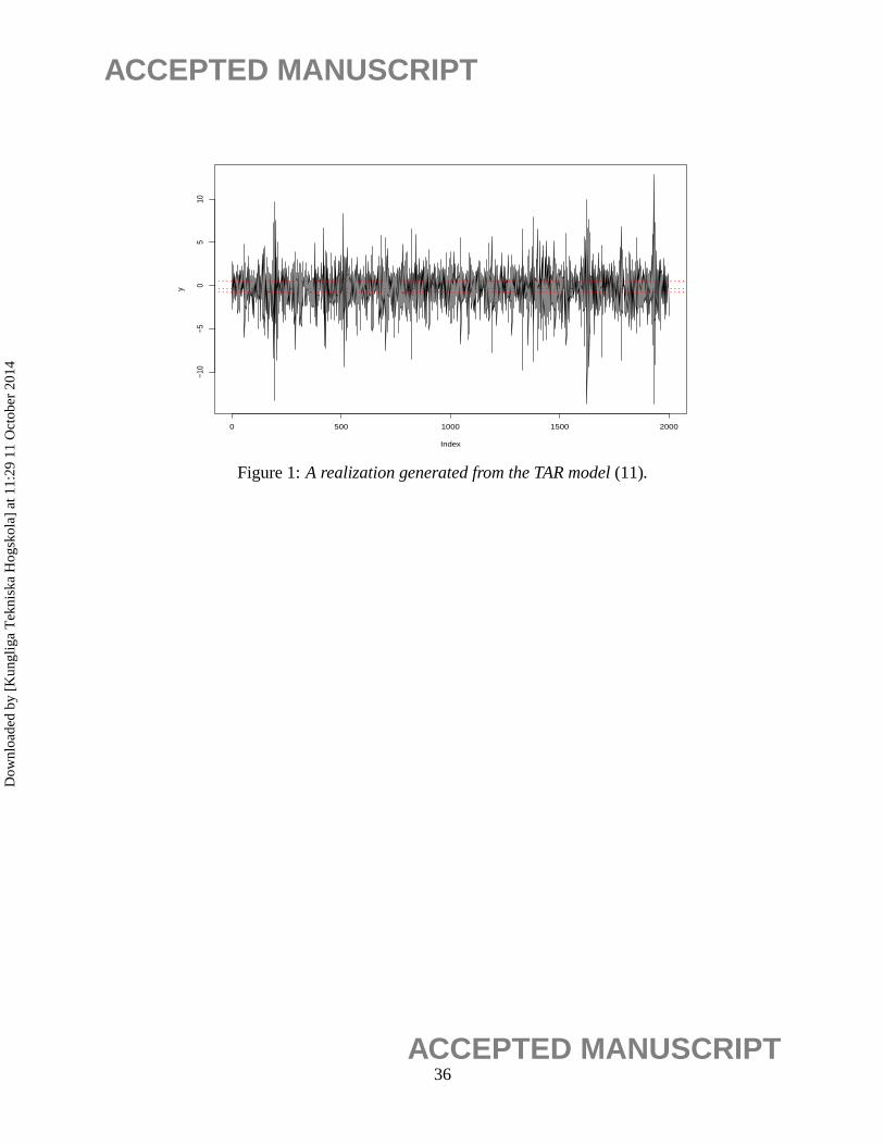
In this first example a series is of length 2000 is generated from the four-regime TAR model
xt = (0.2xt−1 − 0.48xt−2)I(−∞,−0.8) + (1− 0.9xt−1)I(−0.8,−0.3)
+ (0.4xt−1 + 0.3xt−2 − 1.5xt−3 + 0.5xt−4)I(−0.3,0.5)
+ (1− 1.5xt−1 + 0.5xt−2 − 0.5xt−3)I(0.5,∞) + et,
(11)
whereetiid∼ N(0,1) andI(a,b) = I (a < xt−1 ≤ b).
Figure 1 shows a realization of model (11). We applied the methodology in Section 2 to this
realization and obtained three thresholds located atθ1 = −0.8008,θ2 = −0.3011 andθ3 = 0.5013.
Also, the proposed procedure correctly identified the AR orders ( ˆp1, p2, p3, p4) = (2,1,4,3) for
this realization.
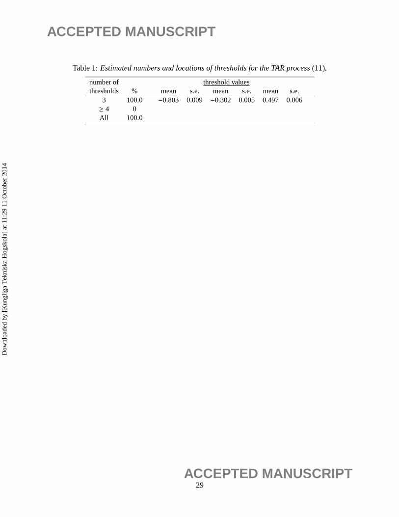
To study the accuracy, we applied the same procedure to 500 realizations of the process (11).
Table 1 lists the percentages of the estimated number of regimes. Note that the number of thresh-
olds are correctly identified in all the 500 realizations. Table 1 also reports the sample means and
standard errors of the three estimated thresholds. All estimated thresholds have small bias and
standard errors.
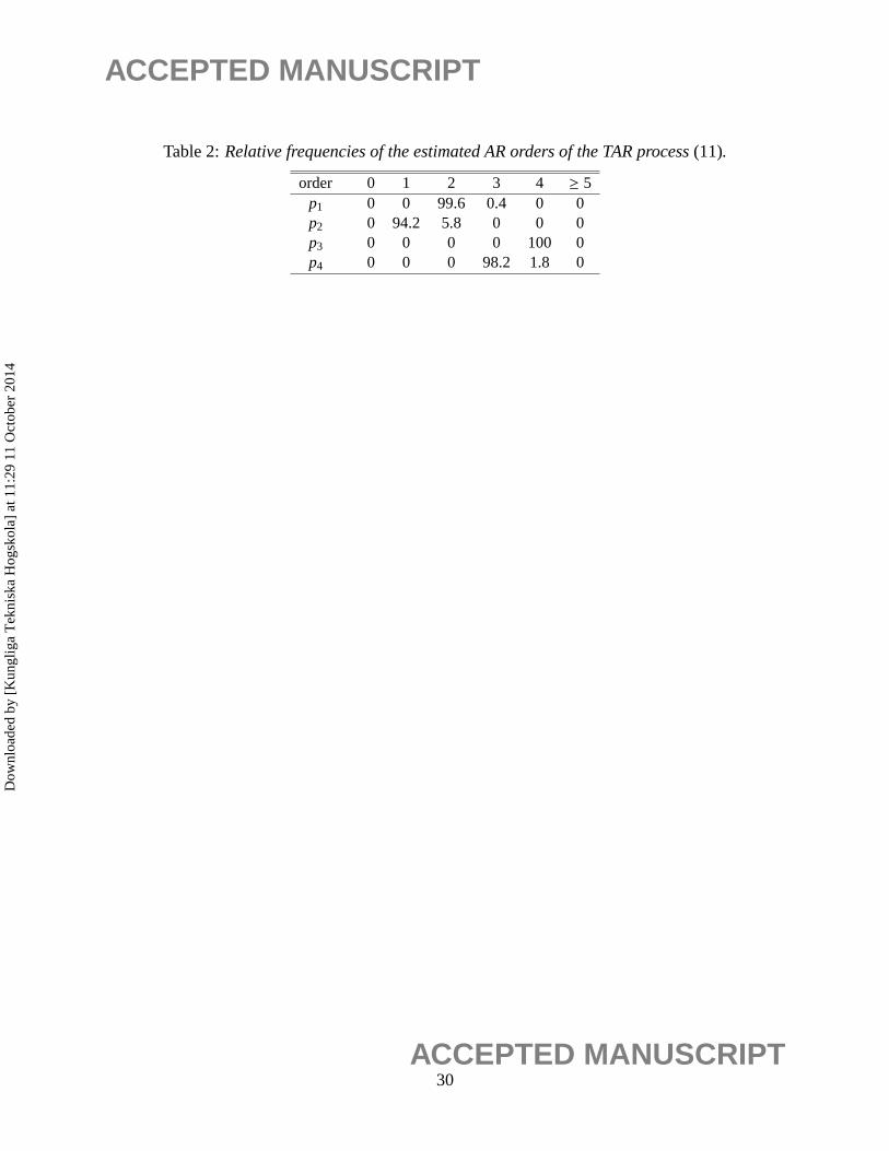
Table 2 summarizes the relative frequencies of the estimated AR orders in the four regimes.
Of the 500 realizations, 94% of them correctly identified the model; i.e., detected three thresholds
with AR orders equal one in all regimes. From Tables 1 and 2, one can see that the proposed
procedure performs very well for the TAR process (11), especially in locating the thresholds.
17ACCEPTED MANUSCRIPT
Dow
nloa
ded
by [
Kun
glig
a T
ekni
ska
Hog
skol
a] a
t 11:
29 1
1 O
ctob
er 2
014
ACCEPTED MANUSCRIPT
4.2 TAR Model With Structural Breaks
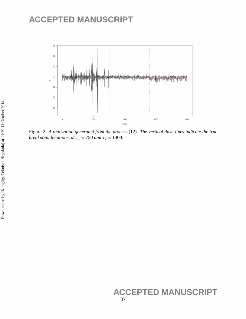
In the second example, we focus on a more complicated model with structural breaks and more
regimes in the TAR models within the segments. The model is
xt =
(−0.7xt−1 − 0.9xt−2 + 0.2xt−3) ∙ I(−∞,−0.8) + (0.8xt−1 − 0.3xt−2) ∙ I(−0.8,−0.3)
−1.25xt−1 ∙ I(−0.3,∞) + et, 1 ≤ t ≤ 750,
(0.5xt−1 − 0.3xt−2) ∙ I(−∞,−1) − 0.6xt−1 ∙ I(−1,∞) + et, 750< t ≤ 1400,
(0.9xt−1 − 0.3xt−2) ∙ I(−∞,0.5) − 2xt−1 ∙ I(0.5,∞) + et, 1400< t ≤ 2000.
(12)
whereetiid∼ N(0,1) and I(a,b) = I (a < xt−1 ≤ b). A realization of (12) is plotted in Figure 2.
Again, 500 realizations from the process (12) are simulated and estimated. Table 3 summarizes the
results of the structural break estimation, including the number of breaks and the sample mean and
standard deviation of the estimated breakpoints when the number of breaks was correctly specified.
The number of breakpoints were correctly identified in all of the 500 realizations.
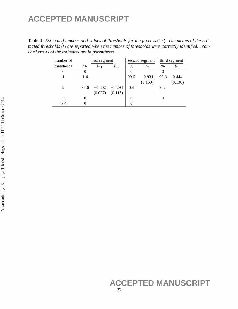
Lastly we investigate the results of threshold estimation for the cases where the number of
breakpoints were correctly identified. Table 4 summarizes the estimation results for the TAR mod-
els in each of the three segments. Despite the complexity of the model, of the 500 realizations, 98%
have simultaneously identified the correct numbers of structural breaks and the correct numbers of
thresholds in all segments.
4.3 Nonlinearity and Nonstationarity
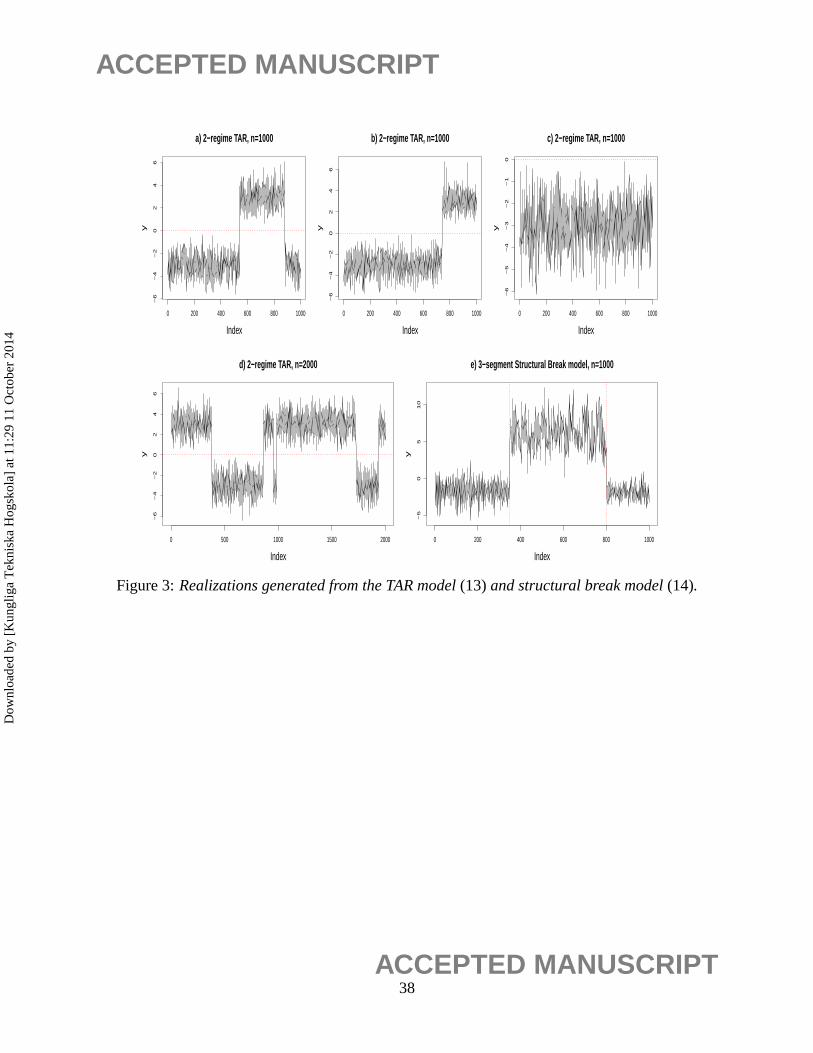
In this last example we illustrate the behavior of the MDL model selection procedure on nonlinear
and nonstationary time series. Consider the following two-regime TAR model
xt = 3I (xt−1 > 0)− 3I (xt−1 ≤ 0)+ et , (13)
whereetiid∼ N(0,1). Figure 3a) shows a realization generated from this model. Notice that this
realization could be easily mis-interpreted as generated from a nonstationary model with two
18ACCEPTED MANUSCRIPT
Dow
nloa
ded
by [
Kun
glig
a T
ekni
ska
Hog
skol
a] a
t 11:
29 1
1 O
ctob
er 2
014
ACCEPTED MANUSCRIPT
breakpoints, although it was originated from the stationary pure threshold model (13). For this
realization, the methodology in Section 2 detected the true two-regime TAR model. This is rea-
sonable because a two-regime model requires coding one threshold and two AR models, which is
simpler than the structural break model that requires coding two breakpoints and three AR models.
Consider another realization of model (13) displayed in Figure 3b). It can be interpreted as
a two-regime TAR model or a structural break model with one breakpoint. Recall that in the
derivation of the MDL criterion, the codelength required to store a breakpoint is log2(τi), while
the code length required to store a threshold is12 log2(ni j ), whereni j is the sample size of the
corresponding regime. Note thatτi = ni j for this realization. Consequently, the penalty associated
with a TAR model is less than the penalty associated with the structural break model. In other
words, the MDL procedure favors a stationary threshold model than a non-stationary structural
break model, which seems to be an attractive feature.
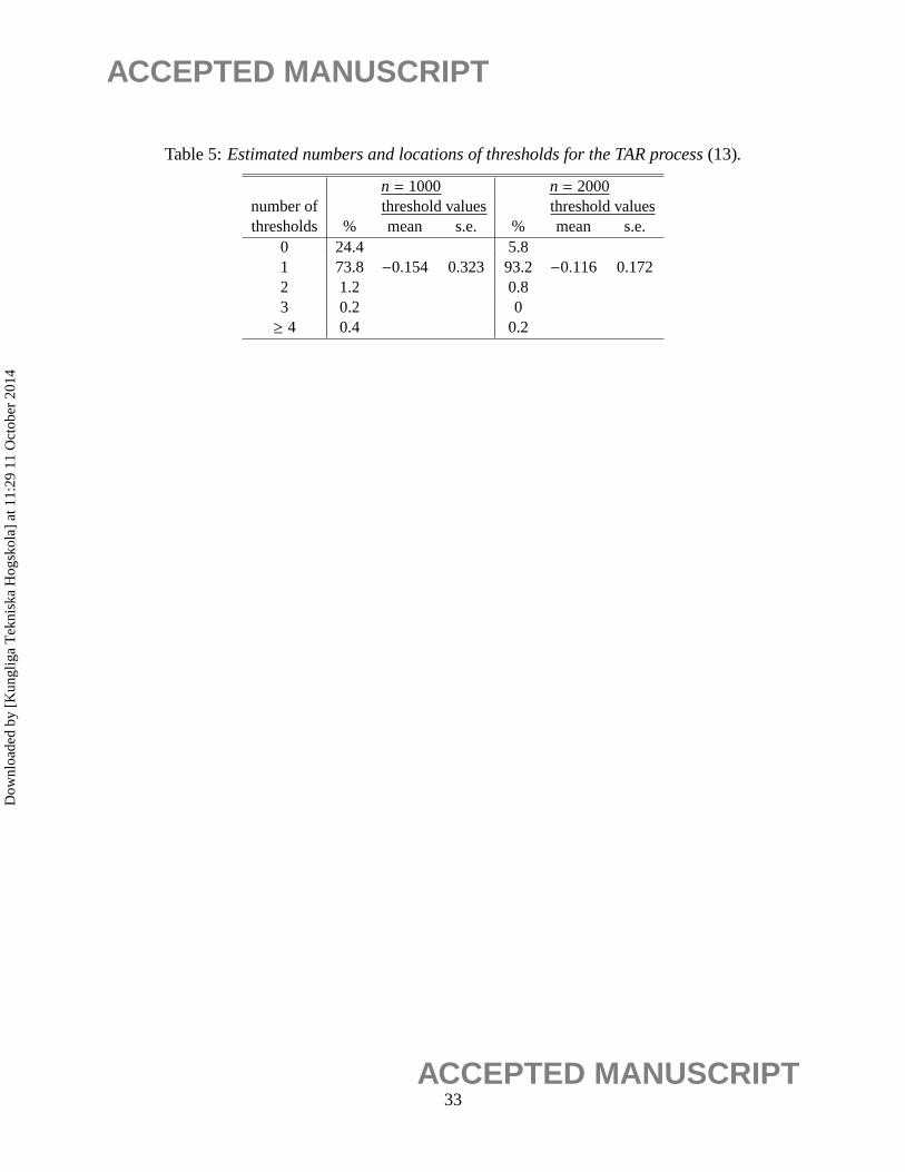
To study the accuracy, we applied the same procedure to 500 realizations of the process (13)
with n = 1000. In all the 500 realizations, no break point was detected. Table 5 lists the percentages
of the estimated number of regimes.
Note that 24.4% of the 500 realizations were mis-classified as no threshold. These correspond
to those cases where no regime switch was present in the entire realization (e.g., see Figure 3c)).
The same experiment was then repeated with sample size increased ton = 2000. With a larger
n, the chance for regime-switching to occur within a realization increases (e.g., see Figure 3d)),
and therefore it can be seen from Table 5 that the percentage of correct model identification was
increased substantially.
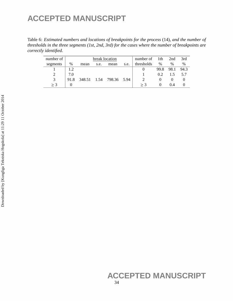
We also studied the pure structural break model
xt =
−3− 0.7xt−1 − 0.3xt−2 + 0.2xt−3 + et, 1 ≤ t ≤ 350,
3+ 0.5xt−1 + et, 350< t ≤ 800,
−2− 0.3xt−1 + 0.2xt−2 + et, 800< t ≤ 1000.
(14)
19ACCEPTED MANUSCRIPT
Dow
nloa
ded
by [
Kun
glig
a T
ekni
ska
Hog
skol
a] a
t 11:
29 1
1 O
ctob
er 2
014
ACCEPTED MANUSCRIPT
We applied the MDL procedure to 500 realizations of this process withn = 1000 and the results
are reported in Table 6. Although the realizations of model (13) and (14) could be very similar
(e.g., see Figure 3a) and Figure 3e)), the first and the third segment in (14) follow different models
and thus they cannot be grouped into the same regime as in (13). It can be seen from Table 6
that the MDL procedure correctly identified the model 90% of the time. In conclusion, the MDL
procedure performed very well in distinguishing between structural break models and threshold
models with few regime switches.
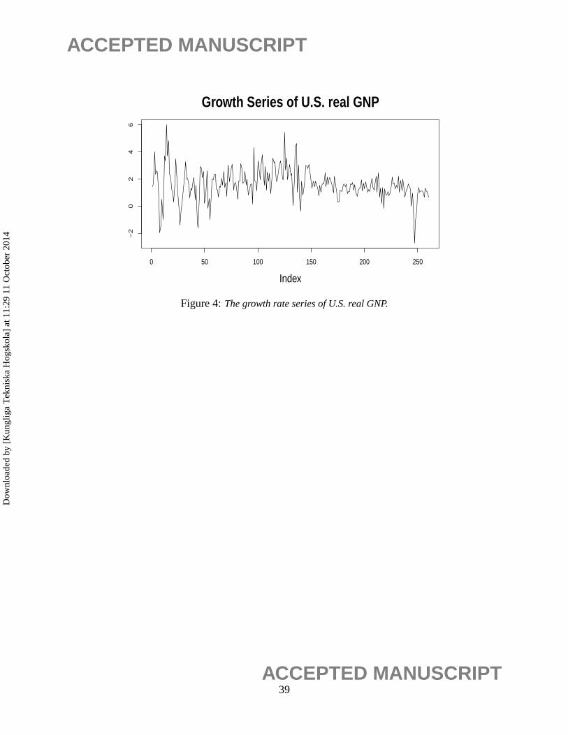
5 Application to U.S. Real GNP Data
In this section, we use the structural break detection procedure developed in Section 3 to study the
growth rate of the quarterly U.S. real GNP data. This data set consists of 261 observations covering
the period 1947-2012, and has been investigated by Li and Ling (2012) using a three-regime TAR
model.
Let y1, . . . , y261 denote the observed real GDP. The growth rate series is defined as
xt = 100(logyt − logyt−1), t = 2, . . . , 260.
The time series plot of the growth rate series{xt} is given in Figure 4. It can be seen that the
series before and after index 150 clearly behave differently, which strongly suggests the presence
of structural breaks in the time series.
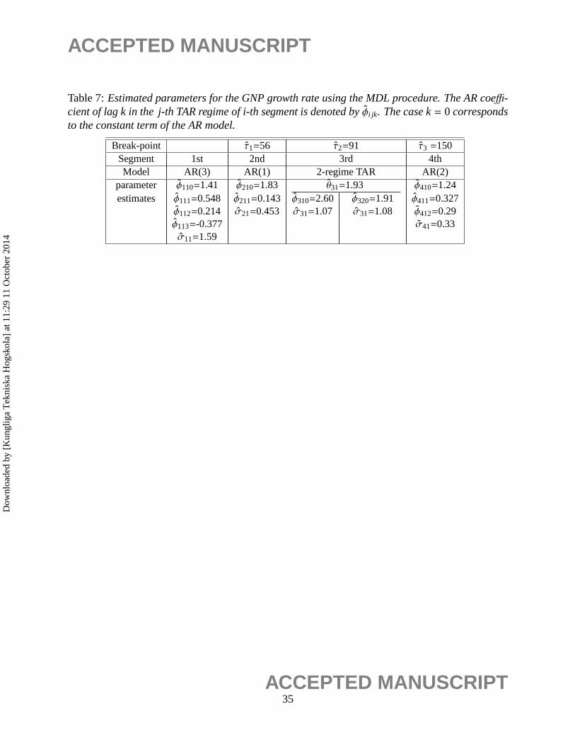
The proposed procedure in Section 3 was applied to this data set, and three structural breaks
were found: ˆτ1 = 56, τ2 = 91, τ3 = 150. Moreover, the fitted results suggest that the first, second
and fourth segments are pure AR models, while the third segment has a thresholds atθ = 1.93.
The details are given in Table 7.
In Li and Ling (2012) this dataset is regarded as a three-regime TAR model without structural
breaks. The fitting of their model and the MDL TAR model fitting with breaks are compared in
20ACCEPTED MANUSCRIPT
Dow
nloa
ded
by [
Kun
glig
a T
ekni
ska
Hog
skol
a] a
t 11:
29 1
1 O
ctob
er 2
014
ACCEPTED MANUSCRIPT
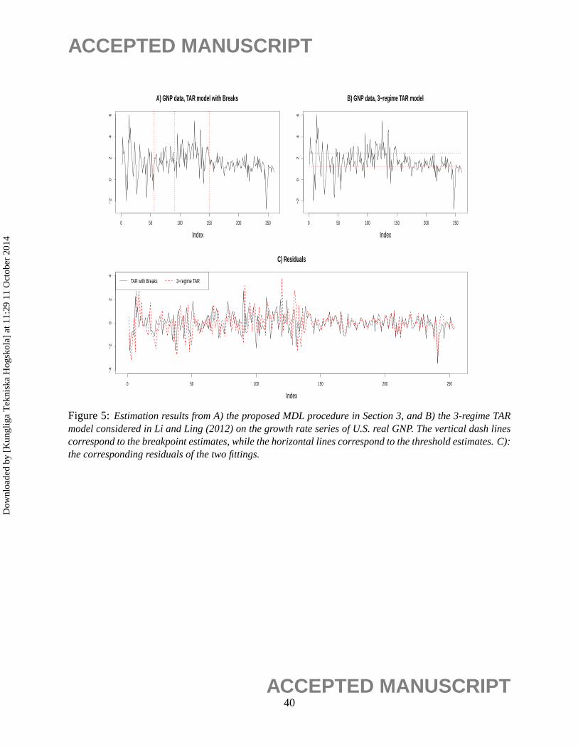
Figure 5. The estimated breakpoints from the MDL procedure appear to partition the time series
into segments with similar behaviors. From the lower half of Figure 3, one can see that the residuals
from both models are similar. In fact, both sets of residuals passed the Ljung-Box test statistic with
p-values approximately equal 0.96, indicating that both models fit the data adequately.
The MDL value corresponds to the three-regime model of Li and Ling (2012) is 295.74. In
each regime of this TAR model, a high order AR model (up to order 10) is required to model
the data, giving the total number of parameters in the model as 31. On the other hand, the MDL
value of our estimated model is 274.13, with a total number of parameters of 21. Moreover, from
Table 7, one can see that simple AR models are sufficient for the data. Thus, given the lower MDL
value and few number of parameters, it appears that a TAR model with structural breaks is a better
parsimonious alternative to describe the GNP data than a pure TAR model.
The estimated structural breaks corresponds to year 1960, 1969 and 1983 respectively. Look-
ing into the history, these three breaks could be associated with substantial changes in the U.S.
economy. For examples, between 1960-1969, the Vietnam war broke out and there were complex
cultural and political disorder across the globe. In the 1980s, there were great changes in business
and economic situations as the production industries migrated to newly industrializing economies.
6 Concluding Remarks
This paper considered the problems of parameter estimation and structural break detection for TAR
models. In particular a new methodology that combines the MDL principle and genetic algorithms
is proposed to handle these tasks. Desirable consistency properties of the parameter estimates are
established. The good finite sample performances of the methodology is illustrated with simulation
experiments and an application to a U.S. GNP data set.
21ACCEPTED MANUSCRIPT
Dow
nloa
ded
by [
Kun
glig
a T
ekni
ska
Hog
skol
a] a
t 11:
29 1
1 O
ctob
er 2
014
ACCEPTED MANUSCRIPT
Acknowledgment
The authors are most grateful to the reviewers, the associate editor and the editor, Professor Xum-
ing He, for their most constructive and helpful comments, which led to a much improved version
of the paper.
A Proof of Theorem 1
This appendix proves Theorem 1. First we define some notations. Following Chan (1993), the
parameter space for the thresholdsθ j, j = 1, . . . , r is taken to be the compact space< = < ∪
{−∞,∞} equipped with the metricd(x, y) = ‖arctan(x) − arctan(y)‖. We assume that the model
parameterΨ j = (σ2j ,Φ j) in the j-th regime belongs to some compact spaceΨ j ∈ <pj+2 for j =
1, . . . , r + 1. Denoteθ = (θ1, . . . , θr) andp = (p1, . . . , pr+1). Also, rewrite the MDL in (7) as
MDL( r, θ, p) = Pen(r,p) +12
r+1∑
j=1
Ln(Ψ( j)n , θ j−1, θ j , pj ,d)
where
Pen(r,p) = log2(r) +r∑
j=1
log2(nj)
2+
r+1∑
j=1
log2(pj) +r+1∑
j=1
pj + 2
2log2(nj)
is the penalty for model complexity and
Ln(Ψ j , θ j−1, θ j , pj ,d) = nj log(2πσ2j ) +
∑nj
t=1(Y( j)t − Φ
′jY
( j)t )2
σ2j
is minus 2 times the conditional log-likelihood for the AR process in thej-th regime; see (5). Here,
Ψ( j)n is the minimizer ofLn(Ψ, θ j−1, θ j , pj ,d) w.r.t.Ψ. Also, for anyθl < θu, define
Q(θl , θu) = E(I (θl < Xt ≤ θu)) ,
L(Ψ, θl , θu, p,d) = limn→∞
1n
E(Ln(Ψ, θl , θu, p,d))
= E
[(
log(2πσ2) +(Xp+1 − Φ′Xp)2
σ2
)
I (θl < Xp+1−d ≤ θu)
]
,
22ACCEPTED MANUSCRIPT
Dow
nloa
ded
by [
Kun
glig
a T
ekni
ska
Hog
skol
a] a
t 11:
29 1
1 O
ctob
er 2
014
ACCEPTED MANUSCRIPT
whereΨ = (σ2,Φ) andXp = (1,Xp, . . . ,X1). Note thatQ gives the expected proportion of sample
size falling into the the regime (θl , θu) andL is the “population version” ofLn. By standard theory
of Kullback-Leibler distance, it can be shown that
L(Ψ, θl , θu, p,d) ≥ L(Ψ( j)0 , θl , θu, p
( j)0 ,d0) (15)
for any (θl , θu) ⊆ (θ( j−1)0 , θ
( j)0 ) and (Ψ, p,d), with equality holds only when (Ψ, p,d) = (Ψ( j)
0 , p( j)0 ,d0)
or ((Ψ( j)0 ,0s), p
( j)0 + s,d0) for any positive integers.
Next we set down some propositions for proving Theorem 1. The proofs of all propositions are
given in Section S.3 of the supplementary file.
Proposition 1. Under Assumption 1, for k= 0,1,2, j = 1, . . . , r + 1 and fixed pj and d,
supθl ,θu,( j)
supΨ j∈Ψ j
∣∣∣∣∣1n
L(k)n (Ψ j , θl , θu, pj ,d) − L(k)(Ψ j , θl , θu, pj ,d)
∣∣∣∣∣a.s.−→ 0 ,
where for k= 1,2, L(k)n represents the k-th derivative of Ln with respective toΨ j , L(0)
n ≡ Ln, and
supθl ,θu,( j) denotes the supremum taken over(θl , θu) ⊆ (θ( j−1)0 − hn, θ
( j)0 + kn) and |θu − θl | > εθ for any
positive sequence hn and kn that are converging to0 as n→ ∞.
For fixedp, d andθl < θu, define
Ψn ≡ Ψn(θl , θu, p,d) = arg minΨ
Ln(Ψ, θl , θu, p,d) ,
Ψ∗ ≡ Ψ∗(θl , θu, p,d) = arg minΨ
L(Ψ, θl , θu, p,d) .
The next proposition shows that the estimated AR coefficients using a proportion of data inside a
segment still converge to the true value.
Proposition 2. Suppose that Assumption 1 holds. Then, for j= 1, . . . , r + 1 and fixed p, d,
supθl ,θu,( j)
∣∣∣Ψn(θl , θu, p,d) − Ψ∗(θl , θu, p,d)∣∣∣
a.s.−→ 0 .
In particular, given that d= d0, thenΨ∗ = Ψ( j)0 if p = p( j)
0 , andΨ∗ = (Ψ( j)0 ,0m) if p − p( j)
0 = m> 0.
23ACCEPTED MANUSCRIPT
Dow
nloa
ded
by [
Kun
glig
a T
ekni
ska
Hog
skol
a] a
t 11:
29 1
1 O
ctob
er 2
014
ACCEPTED MANUSCRIPT
The next proposition shows that the number of thresholds and the AR order in each regime
cannot be underestimated.
Proposition 3. Under Assumption 1, we have
a) The number of thresholds cannot be underestimated, i.e.,rn ≥ r0 a.s.. Also,
maxi=1,...,r0
minj=1,...,rn
|θ( j)n − θ
(i)0 |
a.s.−→ 0 . (16)
b) If the j-th estimated regime is nested in the i-th true regime, thendn → d0 and p( j)n ≥ p(i)
0
almost surely.
The next proposition follows from similar arguments used to derive equation (4.4) of Chan
(1993).
Proposition 4. For any j = 1, . . . , r, ε > 0 andη > 0, there exist some K> 0 andΔ ∈ (0,1) such
that for sufficiently large n,
P
supΔ≥z>K/n
∣∣∣∣∣∣∣
n∑
t=d0+1
ytI (θ( j)0 < Xt−d0 ≤ θ
( j)0 + z)/(nQ(θ( j)
0 , θ( j)0 + z)) − y
∣∣∣∣∣∣∣< η
> 1− ε , (17)
where(yt, y) = (1,1), (et,0), (Xt−ket,0) or (e2t , σ
2j+1) for k = 1, . . . , p. Also, similar conclusions
(with (e2t , σ
2j+1) replaced by(e2
t , σ2j )) hold if (θ( j)
0 , θ( j)0 + z) is replaced by(θ( j)
0 − z, θ( j)0 ). It follows that
for some c> 0,
P
supΔ≥z>cn−1
n∑
t=dn+1
(lt(Ψ
( j+1)n ) − lt(Ψ
( j)n )
)I (θ( j)
0 < Xt−dn≤ θ( j)
0 + z) < 0
→ 1 , and (18)
P
supΔ≥z>cn−1
n∑
t=dn+1
(lt(Ψ
( j)n ) − lt(Ψ
( j+1)n )
)I (θ( j)
0 − z< Xt−dn≤ θ( j)
0 ) < 0
→ 1 , (19)
where forΨ = (σ2,Φ), lt(Ψ) = log(σ2) + (Xt − Φ′Xt−1)2/σ2.
Lastly, the following proposition shows that each threshold can be identified by a threshold
estimate around itsn−1 neighborhood. Thus each estimated regime must be nested in one of the
24ACCEPTED MANUSCRIPT
Dow
nloa
ded
by [
Kun
glig
a T
ekni
ska
Hog
skol
a] a
t 11:
29 1
1 O
ctob
er 2
014

ACCEPTED MANUSCRIPT
true regime asymptotically. Also, the estimated AR coefficients converge to the true values at a
n−1/2 rate.
Proposition 5. Suppose that Assumption 1 holds. Then,
maxi=1,...,r0
minj=1,...,rn
|θ( j)n − θ
(i)0 | = Op
(n−1
), (20)
‖Ψ(i′)n − (Ψ(i)
0 ,0s)‖ = Op
(n−
12
), (21)
for i = 1, . . . , r0 + 1 and some s≥ 0, where i′ is the index such that the i′th-piece of estimated
regime is nested inside the i-th true regime.
Proof of Theorem 1. From Propositions 3 and 5, we know that each of the true thresholds is
identified by an estimated threshold in an−1 neighborhood, and the AR orders will not be underes-
timated. Therefore, we only need to show that the number of thresholds or the AR orders are not
overestimated. That is, it suffices to prove that for any integers = 1, . . . ,R− r0 and any sequence
θn = (θ(1)n , . . . , θ
(r0)n ) such that|θ( j)
0 − θ( j)n | = O(n−1) for j = 1, . . . , r0, the quantity
minθ⊃θn
[2n
MDL( r0 + s, θ,p)
]
−2n
MDL0(r0, θn,p0) (22)
is positive with probability approaching 1, where MDL0 denotes the MDL evaluated at the true AR
coefficientsΨ( j)0 s instead of the maximum likelihood estimates, andp = (p(1), ∙ ∙ ∙ , p(r0+s+1)) is any
integer valued vector such thatp(l) ≥ p( j)0 if (θ(l), θ(l+1)) ⊆ (θ( j)
0 , θ( j+1)0 ). Let θn = (θ(1)
n , . . . , θ(r0+s)n ) be
the minimizer for the first term in (22). Note thatθn ⊂ θn by construction. Using Taylor’s series
expansions on the likelihood function, for sufficiently largen, the quantity in (22) can be expressed
as
2n
(Pen(r0 + s, p) − Pen(r0, p0))
+1n
r0+s+1∑
l=1
Ln(Ψ(l)∗ , θ
(l−1)n , θ(l)n , p
(l), d0) −r0+1∑
j=1
Ln(Ψ( j)0 , θ
( j−1)n , θ
( j)n , p
( j)0 , d0)
(23)
+
r0+s+1∑
l=1
(Ψ(l)n − Ψ
(l)∗ )T 1
nL(2)
n (Ψ(l)+ ; θ(l−1)
n , θ(l)n , p(l), d0)(Ψ(l)
n − Ψ(l)∗ ), (24)
25ACCEPTED MANUSCRIPT
Dow
nloa
ded
by [
Kun
glig
a T
ekni
ska
Hog
skol
a] a
t 11:
29 1
1 O
ctob
er 2
014

ACCEPTED MANUSCRIPT
where|Ψ(l)+ − Ψ
(l)∗ | < |Ψ
(l)n − Ψ
(l)∗ |. Note from Proposition 3 that 2(Pen(r0 + s,p) − Pen(r0,p0))/n
is positive and of orderO(logn/n). Using Proposition 2, it follows that the quantity in (23) is
exactly 0 since (Ψ( j)0 , p
( j)0 ) and (Ψ(l)
∗ , p(l)) specify the same model if (θ(l), θ(l+1)) ⊆ (θ( j)0 , θ
( j+1)0 ) and
p(l) ≥ p( j)0 . Also, from Proposition 5, the term in (24) is of orderOp(n−1). Therefore 2(Pen(r0 +
s,p) − Pen(r0,p0))/n, which is of orderO(logn/n), dominates the expression and the quantity in
(22) is indeed positive with probability approaching 1. This completes the proof of Theorem 1.�
References
Alba, E. and Troya, J. M. (1999) A survey of parallel distributed genetic algorithms.Complexity,
4, 31–52.
Alba, E. and Troya, J. M. (2002) Improving flexibility and efficiency by adding parallelism to
genetic algorithms.Statistics and Computing, 12, 91–114.
Aue, A, H. S. H. L. and Reimherr, M. (2009) Break detection in the covariance structure of multi-
variate time series models.The Annals of Statistics, 37, 4046–4087.
Berkes, I., Horvath, L., Ling, S. and Schauer, J. (2011) Testing for structural change of AR model
to threshold AR model.Journal of Time Series Analysis, 32, 547–565.
Chan, K. S. (1993) Consistency and limiting distribution of the least squares estimator of a thresh-
old autoregressive model.The Annals of Statistics, 21, 520–533.
Coakley, J., Fuertes, A.-M. and Perez, M.-T. (2003) Numerical issues in threshold autoregressive
modeling of time series.Journal of Economic Dynamics and Control, 27, 2219–2242.
Davis, R. A., Lee, T. C. M. and Rodriguez-Yam, G. A. (2006) Structural break estimation for
nonstationary time series models.Journal of the American Statistical Association, 101, 223–
239.
26ACCEPTED MANUSCRIPT
Dow
nloa
ded
by [
Kun
glig
a T
ekni
ska
Hog
skol
a] a
t 11:
29 1
1 O
ctob
er 2
014
ACCEPTED MANUSCRIPT
Davis, R. A., Lee, T. C. M. and Rodriguez-Yam, G. A. (2008) Break detection for a class of
nonlinear time series models.Journal of Time Series Analysis, 29, 834–867.
Davis, R. A. and Yau, C. Y. (2013) Consistency of minimum description length model selection
for piecewise stationary time series models.Electronic Journal of Statistics, 7, 381–411.
Gonzalo, J. and Pitarakis, J.-Y. (2002) Estimation and model selection based inference in single
and multiple threshold models.Journal of Econometrics, 110, 319–352.
Hansen, M. H. and Yu, B. (2001) Model selection and the principle of minimum description length.
Journal of the American Statistical Association, 96, 746–774.
Lavielle, M. and Ludena, C. (2000) The multiple change-points problem for the spectral distribu-
tion. Bernoulli, 6, 845–869.
Lee, T. C. M. (2001) An introduction to coding theory and the two-part minimum description
length principle.International Statistical Review, 69, 169–183.
Li, D. and Ling, S. (2012) On the least squares estimation of multiple-regime threshold autoregres-
sive models.Journal of Econometrics, 167, 240–253.
Lu, Q., Lund, R. and Lee, T. C. M. (2010) An MDL approach to the climate segmentation problem.
The Annals of Applied Statistics, 4, 299–319.
Rissanen, J. (1989)Stochastic Complexity in Statistical Inquiry. World Scientific, Singapore.
Rissanen, J. (2007)Information and Complexity in Statistical Modeling. Springer.
Tong, H. (1978) On a threshold model. InPattern Recognition and Signal Processing. NATO ASI
Series E: Applied Sc. (29).(ed. C. Chen), 575–586. Oxford University Press.
Tong, H. (1990)Non-linear Time Series: a Dynamical System Approach. Oxford University Press.
Tong, H. (2011) Threshold models in time series analysis–30 years on.Statistics and its Interface,
4, 107–118.
27ACCEPTED MANUSCRIPT
Dow
nloa
ded
by [
Kun
glig
a T
ekni
ska
Hog
skol
a] a
t 11:
29 1
1 O
ctob
er 2
014
ACCEPTED MANUSCRIPT
Tsay, R. S. (1989) Testing and modeling threshold autoregressive processes.Journal of the Amer-
ican Statistical Association, 84, 231–240.
Zhu, K. and Ling, S. (2012) Likelihood ratio tests for the structural change of an AR(p) model to
a threshold AR(p) model.Journal of Time Series Analysis, 33, 223–232.
28ACCEPTED MANUSCRIPT
Dow
nloa
ded
by [
Kun
glig
a T
ekni
ska
Hog
skol
a] a
t 11:
29 1
1 O
ctob
er 2
014
ACCEPTED MANUSCRIPT
Table 1:Estimated numbers and locations of thresholds for the TAR process(11).
number of threshold valuesthresholds % mean s.e. mean s.e. means.e.
3 100.0 −0.803 0.009 −0.302 0.005 0.497 0.006≥ 4 0All 100.0
29ACCEPTED MANUSCRIPT
Dow
nloa
ded
by [
Kun
glig
a T
ekni
ska
Hog
skol
a] a
t 11:
29 1
1 O
ctob
er 2
014
ACCEPTED MANUSCRIPT
Table 2:Relative frequencies of the estimated AR orders of the TAR process(11).
order 0 1 2 3 4 ≥ 5p1 0 0 99.6 0.4 0 0p2 0 94.2 5.8 0 0 0p3 0 0 0 0 100 0p4 0 0 0 98.2 1.8 0
30ACCEPTED MANUSCRIPT
Dow
nloa
ded
by [
Kun
glig
a T
ekni
ska
Hog
skol
a] a
t 11:
29 1
1 O
ctob
er 2
014

ACCEPTED MANUSCRIPT
Table 3:Estimated numbers and locations of breakpoints for the process(12).
number of breaklocationsegments % mean s.e. mean s.e.
3 100 750.51 8.55 1401.8714.58
31ACCEPTED MANUSCRIPT
Dow
nloa
ded
by [
Kun
glig
a T
ekni
ska
Hog
skol
a] a
t 11:
29 1
1 O
ctob
er 2
014
ACCEPTED MANUSCRIPT
Table 4:Estimated number and values of thresholds for the process(12). The means of the esti-mated thresholdsθi j are reported when the number of thresholds were correctly identified. Stan-dard errors of the estimates are in parentheses.
number of first segment second segment third segmentthresholds % θ11 θ12 % θ21 % θ31
0 0 0 01 1.4 99.6 −0.931 99.8 0.444
(0.150) (0.130)2 98.6 −0.802 −0.294 0.4 0.2
(0.027) (0.115)3 0 0 0≥ 4 0 0
32ACCEPTED MANUSCRIPT
Dow
nloa
ded
by [
Kun
glig
a T
ekni
ska
Hog
skol
a] a
t 11:
29 1
1 O
ctob
er 2
014
ACCEPTED MANUSCRIPT
Table 5:Estimated numbers and locations of thresholds for the TAR process(13).
n = 1000 n = 2000numberof threshold values threshold valuesthresholds % mean s.e. % mean s.e.
0 24.4 5.81 73.8 −0.154 0.323 93.2 −0.116 0.1722 1.2 0.83 0.2 0≥ 4 0.4 0.2
33ACCEPTED MANUSCRIPT
Dow
nloa
ded
by [
Kun
glig
a T
ekni
ska
Hog
skol
a] a
t 11:
29 1
1 O
ctob
er 2
014
ACCEPTED MANUSCRIPT
Table 6:Estimated numbers and locations of breakpoints for the process(14), and the number ofthresholds in the three segments (1st, 2nd, 3rd) for the cases where the number of breakpoints arecorrectly identified.
numberof breaklocation number of 1th 2nd 3rdsegments % mean s.e. mean s.e. thresholds % % %
1 1.2 0 99.8 98.1 94.32 7.0 1 0.2 1.5 5.73 91.8 348.51 1.54 798.365.94 2 0 0 0≥ 3 0 ≥ 3 0 0.4 0
34ACCEPTED MANUSCRIPT
Dow
nloa
ded
by [
Kun
glig
a T
ekni
ska
Hog
skol
a] a
t 11:
29 1
1 O
ctob
er 2
014
ACCEPTED MANUSCRIPT
Table 7:Estimated parameters for the GNP growth rate using the MDL procedure. The AR coeffi-cient of lag k in the j-th TAR regime of i-th segment is denoted byφi jk . The case k= 0 correspondsto the constant term of the ARmodel.
Break-point ˆτ1=56 τ2=91 τ3 =150Segment 1st 2nd 3rd 4thModel AR(3) AR(1) 2-regime TAR AR(2)
parameter φ110=1.41 φ210=1.83 θ31=1.93 φ410=1.24estimates φ111=0.548 φ211=0.143 φ310=2.60 φ320=1.91 φ411=0.327
φ112=0.214 σ21=0.453 σ31=1.07 σ31=1.08 φ412=0.29φ113=-0.377 σ41=0.33σ11=1.59
35ACCEPTED MANUSCRIPT
Dow
nloa
ded
by [
Kun
glig
a T
ekni
ska
Hog
skol
a] a
t 11:
29 1
1 O
ctob
er 2
014
ACCEPTED MANUSCRIPT
0 500 1000 1500 2000
−10
−50
510
Index
y
Figure 1:A realization generated from the TAR model(11).
36ACCEPTED MANUSCRIPT
Dow
nloa
ded
by [
Kun
glig
a T
ekni
ska
Hog
skol
a] a
t 11:
29 1
1 O
ctob
er 2
014
ACCEPTED MANUSCRIPT
0 500 1000 1500 2000
−3
0−
20
−1
00
10
20
30
Index
y
Figure 2:A realization generated from the process(12). The vertical dash lines indicate the truebreakpoint locations, atτ1 = 750andτ2 = 1400.
37ACCEPTED MANUSCRIPT
Dow
nloa
ded
by [
Kun
glig
a T
ekni
ska
Hog
skol
a] a
t 11:
29 1
1 O
ctob
er 2
014
ACCEPTED MANUSCRIPT
0 200 400 600 800 1000
−6
−4
−2
02
46
a) 2−regime TAR, n=1000
Index
y
0 200 400 600 800 1000
−6
−4
−2
02
46
b) 2−regime TAR, n=1000
Indexy
0 200 400 600 800 1000
−6
−5
−4
−3
−2
−1
0
c) 2−regime TAR, n=1000
Index
y
0 500 1000 1500 2000
−6
−4
−2
02
46
d) 2−regime TAR, n=2000
Index
y
0 200 400 600 800 1000
−5
05
10
e) 3−segment Structural Break model, n=1000
Index
y
Figure 3:Realizations generated from the TAR model(13)and structural break model(14).
38ACCEPTED MANUSCRIPT
Dow
nloa
ded
by [
Kun
glig
a T
ekni
ska
Hog
skol
a] a
t 11:
29 1
1 O
ctob
er 2
014
ACCEPTED MANUSCRIPT
Growth Series of U.S. real GNP
Index
0 50 100 150 200 250
−2
02
46
Figure 4:The growth rate series of U.S. real GNP.
39ACCEPTED MANUSCRIPT
Dow
nloa
ded
by [
Kun
glig
a T
ekni
ska
Hog
skol
a] a
t 11:
29 1
1 O
ctob
er 2
014
ACCEPTED MANUSCRIPT
A) GNP data, TAR model with Breaks
Index
0 50 100 150 200 250
−2
02
46
B) GNP data, 3−regime TAR model
Index
0 50 100 150 200 250
−2
02
46
C) Residuals
Index
0 50 100 150 200 250
−4
−2
02
4
TAR with Breaks 3−regime TAR
Figure 5:Estimation results from A) the proposed MDL procedure in Section 3, and B) the 3-regime TARmodel considered in Li and Ling (2012) on the growth rate series of U.S. real GNP. The vertical dash linescorrespond to the breakpoint estimates, while the horizontal lines correspond to the threshold estimates. C):the corresponding residuals of the two fittings.
40ACCEPTED MANUSCRIPT
Dow
nloa
ded
by [
Kun
glig
a T
ekni
ska
Hog
skol
a] a
t 11:
29 1
1 O
ctob
er 2
014