estimation of long memory in volatility using wavelets

Institute of Economic Studies, Faculty of Social Sciences

Charles University in Prague

Estimation of Long Memory

in Volatility Using Wavelets

Jozef Baruník

Lucie Kraicová

IES Working Paper: 33/2014

Institute of Economic Studies, Faculty of Social Sciences,

Charles University in Prague

[UK FSV – IES]

Opletalova 26

CZ-110 00, Prague E-mail : [email protected]

http://ies.fsv.cuni.cz

Institut ekonomických studií

Fakulta sociálních věd

Univerzita Karlova v Praze

Opletalova 26

110 00 Praha 1

E-mail : [email protected]

http://ies.fsv.cuni.cz

Disclaimer: The IES Working Papers is an online paper series for works by the faculty and students of the Institute of Economic Studies, Faculty of Social Sciences, Charles University in Prague, Czech Republic. The papers are peer reviewed, but they are not edited or formatted by the

editors. The views expressed in documents served by this site do not reflect the views of the IES or any other Charles University Department. They are the sole property of the respective authors. Additional info at: [email protected]

Copyright Notice: Although all documents published by the IES are provided without charge, they are licensed for personal, academic or educational use. All rights are reserved by the authors.

Citations : All references to documents served by this site must be appropriately cited.

Bibliographic information: Baruník J., Kraicová L. (2014). “Estimation of Long Memory in Volatility Using Wavelets” IES Working Paper 33/2014. IES FSV. Charles University.

This paper can be downloaded at: http://ies.fsv.cuni.cz

mailto:[email protected]

http://ies.fsv.cuni.cz/





Estimation of Long Memory in

Volatility Using Wavelets

Jozef Baruníka

Lucie Kraicováb

aInstitute of Economic Studies, Faculty of Social Sciences, Charles University in

Prague, Smetanovo nábreží 6, 111 01 Prague 1, Czech Republic

email: kraicova.1 @seznam.cz bInstitute of Information Theory and Automation, Academy of Sciences of the Czech

Republic: Pod Vodarenskou Vezi 4, 182 00, Prague, Czech Republic

email: [email protected]

September 2014

Abstract:

This work studies wavelet-based Whittle estimator of the Fractionally Integrated

Exponential Generalized Autoregressive Conditional Heteroscedasticity

(FIEGARCH) model often used for modeling long memory in volatility of financial

assets. The newly proposed estimator approximates the spectral density using

wavelet transform, which makes it more robust to certain types of irregularities in

data. Based on an extensive Monte Carlo study, both behavior of the proposed

estimator and its relative performance with respect to traditional estimators are

assessed. In addition, we study properties of the estimators in presence of jumps,

which brings interesting discussion. We find that wavelet-based estimator may

become an attractive robust and fast alternative to the traditional methods of

estimation.

Keywords: volatility, long memory, FIEGARCH, wavelets, Whittle, Monte Carlo

JEL: C13, C18, C51, G17

Acknowledgements: We would like to express our gratitude to Ana Perez, who

provided us with the code for MLE and FWE estimation of FIEGARCH processes,

and we gratefully acknowledge _nancial support from the the Czech Science

Foundation under project No. 13-32263S. Please note that the Online Appendix to

this manuscript is available for download at http://ies.fsv.cuni.cz/en/staff/kraicova.



1 Introduction

During past decades, volatility has became one of the most extensively studied variables infinance. This enormous interest has mainly been spurred by the importance of volatilityas a measure of risk for both academics and practitioners. Despite numerous modelingand estimation approaches developed in the literature, there are many interesting aspectsof estimation waiting for further research. One area of lively discussions is estimation ofparameters in long memory models led by the desire to capture persistence of volatility timeseries. This persistence belongs to the important stylized facts, as it implies that shock inthe volatility will impact future volatility over a long horizon. The FI(E)GARCH extension(Bollerslev & Mikkelsen, 1996) to the original (G)ARCH modeling framework of Engle (1982);Bollerslev (1986) was shown to capture this empirically observed correlation well. In ourwork, we contribute to the discussion with interesting alternative estimation framework forthe FIEGARCH model based on wavelet approximation of likelihood function.

Although traditional maximum likelihood (ML) framework for estimation of parametersis desirable due to its efficiency, an alternative approach, Whittle estimator can be employed(Zaffaroni, 2009). The Whittle estimator is obtained by maximizing frequency domain ap-proximation of the Gaussian likelihood function, the so-called Whittle function (Whittle,1962), and although it can not attain better efficiency, it may serve as a computationally fastalternative to ML for complex optimization problems.

Traditionally, Whittle estimators use likelihood approximations based on Fourier trans-form. Whereas this is accurate alternative to be used in many applications, in finance,non-stationarities and significant time-localized patterns in data can emerge. Jensen (1999)provides an alternative type of estimation based on approximation of likelihood function us-ing wavelets. The main advantage of applying wavelet-based Whittle estimator in volatilitymodeling is that wavelets are time localized and can better approximate spectral density incase of non-stationarities found in volatility process.

Compared to the wide range of studies on semi-parametric Wavelet Whittle estimators(for relative performance of local FWE and WWE of ARFIMA model see e.g. Fay et al. (2009)or Frederiksen & Nielsen (2005) and related works), literature assessing performance of theirparametric counterparts is not extensive. Though, results of the studies completed so farsuggest that the performance of WWE in parametric setting is an interesting and importantresearch topic. Jensen (1999) introduces wavelet Whittle estimation (WWE) of ARFIMAprocess, and compares its performance with traditional Fourier-based Whittle estimator. Hefinds that estimators perform similarly, with an exception of MA coefficients being close toboundary of invertibility of the process. In this case, Fourier-based estimation deteriorates,whereas wavelet-based estimation retains its accuracy. Percival & Walden (2000) describe awavelet-based approximate MLE for both stationary and non-stationary fractionally differ-enced processes, and demonstrates its relatively good performance on very short samples (128observations). Whitcher (2004) applies WWE based on a discrete wavelet packet transform(DWPT) to a seasonal persistent process and again finds good performance of this estima-

2

tion strategy. Heni & Mohamed (2011) apply this strategy on a FIGARCH-GARMA model,further application can be seen in Gonzaga & Hauser (2011).

Literature focusing on WWE studies various models, but estimation of FIEGARCHhas not been fully explored yet with exception of Perez & Zaffaroni (2008) and Zaffaroni(2009). These authors successfully applied traditional Fourier-based Whittle estimators ofFIEGARCH models, and found that Whittle estimates perform better in comparison to MLin cases of processes close to being non-stationary. Authors found that while ML is oftenmore efficient alternative, FWE outperforms it in terms of bias mainly in case of high per-sistence of the processes. Hence Whittle type of estimators seem to offer lower bias at costof lower efficiency.

In our work, we contribute to the literature by extending the study of Perez & Zaffaroni(2008) using wavelet-based Whittle estimator (Jensen, 1999). The newly introduced WWEis based on two alternative approximations of likelihood function. Following the work ofJensen (1999), we propose to use discrete wavelet transform (DWT) in approximation ofFIEGARCH likelihood function, and alternatively, we use maximal overlap discrete wavelettransform (MODWT). In an experiment setup mirroring that of Perez & Zaffaroni (2008),we focus on studying small sample performance of the newly proposed estimators, and guid-ing potential users of the estimators through practical aspects of estimation. To study bothsmall sample properties of the estimator and its relative performance to traditional estima-tion techniques under different situations, we run extensive Monte Carlo experiments. Acompeting estimators are Fourier-based Whittle estimator (FWE), and traditional maximumlikelihood estimator (MLE). In addition, we also study the performance of estimators underthe presence of jumps in the processes.

Our results show that even in the case of simulated data, which follow a pure FIEGARCHprocess, and thus do not allow to fully utilize the advantages of WWE over its traditionalcounterparts, the estimator performs reasonably well. When we focus on the individual pa-rameters estimation, in terms of bias the performance is comparable to traditional estimators,in some cases outperforming FWE, while in terms of efficiency the latter is usually better.In terms of forecasting performance, the differences are even smaller. The exact MLE mostlyoutperforms both of the Whittle estimators in terms of efficiency, with just rare exceptions.Yet, due to the computational complexity of the MLE in case of large data sets, FWE andWWE thus represent an attractive fast alternatives for parameter estimation.

The rest of the text is structured as follows: section 2 introduces the FIEGARCH modeland the individual estimators; in section 3 the setup of the Monte Carlo experiment is de-scribed and results are discussed. Due to the extend of the results, we relegate all support-ing results to the online appendix available for download at http://ies.fsv.cuni.cz/en/

staff/kraicova. In section 4 we present the extended experiment; in section 5 we compareour results with related literature; section 6 concludes.

3

http://ies.fsv.cuni.cz/en/staff/kraicova

http://ies.fsv.cuni.cz/en/staff/kraicova

2 Estimation Frameworks for FIEGARCH(q, d, p)

2.1 FIEGARCH(q, d, p) Process

Despite the extremely wide spectrum of processes generating financial returns time series,there are some stylized features which many of them have in common. They have beendetected over years of financial market analysis and have shaped the means of financial timeseries modeling. One of the main features, the time-variant dependence in volatility led todevelopment of conditional volatility models by Engle (1982). Over time, performance of thesemodels (ARCH family models) in practical applications has demonstrated the importance ofconditional volatility in time series analysis and feasibility of direct volatility estimationand forecasting. Although several alternative concepts based on explicitly modeled volatilityhave been developed since Engle (1982), generalized ARCH models are still among those bestperforming in practical applications. This makes it relevant to study the performance of newparameter estimators in their context. In our study we focus on one of the generalizationsof the ARCH model, the FIEGARCH(q, d, p), where the log-returns {εt}Tt=1 are modeledconditionally on their past realizations as:

εt = zth1/2t (1)

ln(ht) = ω + Φ(L)g(zt−1) (2)

g(zt) = θzt + γ[|zt| − E(|zt|)], (3)

where zt is an N (0, 1) independent identically distributed (i.i.d.) unobservable innovationsprocess, εt is observable discrete-time real valued process with conditional log-variance processdependent on the past innovations Et−1(ε2t ) = ht, and L is a lag operator Ligt = gt−i inΦ(L) = (1−L)−d[1 +α(L)][β(L)]−1. The polynomials α(L) = 1 +α[2](L) = 1 +

∑pi=2 αiL

i−1

and β(L) = 1 −∑q

i=1 βiLi have no zeros in common, their roots are outside the unit circle,

θγ 6= 0 and d < 0.5. (1− L)d = 1− d∑∞

k=1 Γ(k − d)Γ(1− d)−1Γ(k + 1)−1Lk with Γ(.) beinggamma function.

Any FIEGARCH(q, d, p) process is then fully determined by the number of parameters,their values and distribution of the standardized innovations zt. Concerning the last factor,the three most frequent assumptions in the literature are the standard normal distributionproviding a convenient estimation environment, student-t distribution assuming thicker tails,and Generalized Error Distribution (GED) with parameter v determining the tail thickness.Normal distribution is nested as a special case of GED for v = 2.

The model captures importnant stylized features of the real financial time series data;short-term temporal variation in financial returns volatility (volatility clustering), long-termtemporal variation in financial returns volatility (long memory), negative relationship betweenpast returns and volatility (leverage effect) and fat-tailed sample distribution of returns.We provide plots of a FIEGARCH process with three different levels of long memory forillustration in Section ?? of an online appendix.

While correct model specification is important for capturing all the empirical features

4

of the data, feasibility of estimation of its parameters is crucial. In general, estimation ofthe FIEGARCH model can be carried out by various methods. Below, those considered inthis work (the benchmark estimators MLE and FWE, and the newly introduced WWE) aredescribed together with practical aspects of their application.

2.2 (Quasi) Maximum Likelihood Estimator

The Maximum Likelihood Estimation is often considered the gold-standard for parameter es-timation, hence it serves as a natural benchmark estimation framework used in this study. Fora general zero mean, stationary Gaussian process {xt}Tt=1, the maximum likelihood estimator(MLE) is defined as

ζMLE = argminζ∈Θ

LMLE(ζ), (4)

where LMLE(ζ) is the negative log-likelihood function

LMLE(ζ) =T

2ln(2π) +

12

ln |ΣT |+12(x′tΣ

−1T xt

), (5)

where ΣT is the covariance matrix of xt, |ΣT | is its determinant and ζ is the vector ofparameters to be estimated.

Despite the favorable properties of the MLE, there are some issues limiting its practicalapplicability. The usual problem is that we have to deal with the inversion of the covariancematrix of the process and with its determinant. Although it may not be a problem when thematrix is diagonal or sufficiently sparse, in cases of dense covariance matrices (characteristicfor long memory processes) it may be extremely time demanding, or even unfeasible in caseof large datasets. Moreover, as discussed in (Beran (1994), chapter 5), solution may be evenunstable in the presence of long memory, when the covariance matrix is close to singularity.Next, empirical data often does not to have zero mean, hence the mean has to be estimatedand deducted. The efficiency and bias of the estimator of the mean contributes to theefficiency and bias of the MLE. In case of long-memory processes it can cause significantdeterioration of the MLE (Cheung & Diebold, 1994). Both these issues have motivatedconstruction of alternative estimators, usually formulated as approximate MLE and definedby an approximated log-likelihood function (Beran, 1994; Nielsen & Frederiksen, 2005).

Since the assumption of a specific distribution is usually too restrictive for practical ap-plications, it is important to study the estimator in situations when it is constructed for someprocess but applied to a different process. In the context of GARCH processes with non-normal error distribution, Quasi-Maximum Likelihood Estimator (QMLE) has been studiedby Bollerslev & Wooldridge (1992), who show that the estimator remains consistent, but losesefficiency. The efficiency loss, as argued in Engle & Gonzalez-Rivera (1991), is rather smallfor symmetric t-distributed processes, but can be significant under asymmetric distribution.As discussed in Bollerslev & Wooldridge (1992), standard test statistics become biased and toensure valid inference, their robustified counterparts, such as those proposed by the authors,

5

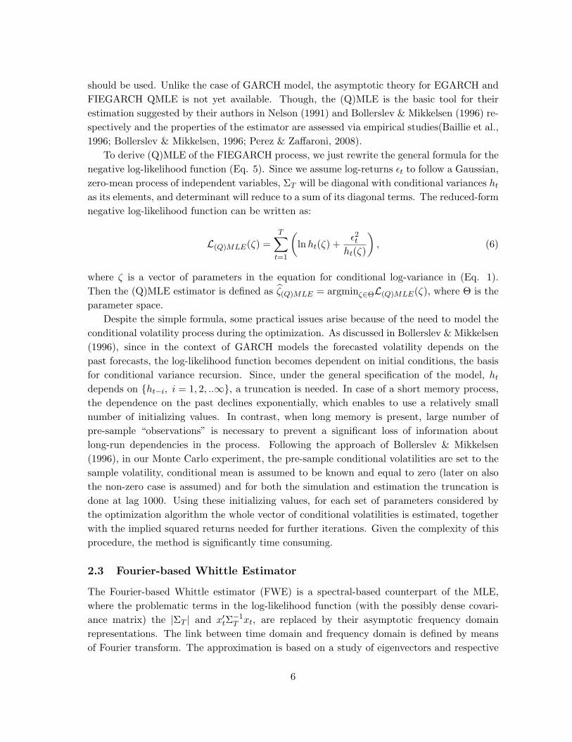
should be used. Unlike the case of GARCH model, the asymptotic theory for EGARCH andFIEGARCH QMLE is not yet available. Though, the (Q)MLE is the basic tool for theirestimation suggested by their authors in Nelson (1991) and Bollerslev & Mikkelsen (1996) re-spectively and the properties of the estimator are assessed via empirical studies(Baillie et al.,1996; Bollerslev & Mikkelsen, 1996; Perez & Zaffaroni, 2008).

To derive (Q)MLE of the FIEGARCH process, we just rewrite the general formula for thenegative log-likelihood function (Eq. 5). Since we assume log-returns εt to follow a Gaussian,zero-mean process of independent variables, ΣT will be diagonal with conditional variances htas its elements, and determinant will reduce to a sum of its diagonal terms. The reduced-formnegative log-likelihood function can be written as:

L(Q)MLE(ζ) =T∑t=1

(lnht(ζ) +

ε2tht(ζ)

), (6)

where ζ is a vector of parameters in the equation for conditional log-variance in (Eq. 1).Then the (Q)MLE estimator is defined as ζ(Q)MLE = argminζ∈ΘL(Q)MLE(ζ), where Θ is theparameter space.

Despite the simple formula, some practical issues arise because of the need to model theconditional volatility process during the optimization. As discussed in Bollerslev & Mikkelsen(1996), since in the context of GARCH models the forecasted volatility depends on thepast forecasts, the log-likelihood function becomes dependent on initial conditions, the basisfor conditional variance recursion. Since, under the general specification of the model, htdepends on {ht−i, i = 1, 2, ..∞}, a truncation is needed. In case of a short memory process,the dependence on the past declines exponentially, which enables to use a relatively smallnumber of initializing values. In contrast, when long memory is present, large number ofpre-sample “observations” is necessary to prevent a significant loss of information aboutlong-run dependencies in the process. Following the approach of Bollerslev & Mikkelsen(1996), in our Monte Carlo experiment, the pre-sample conditional volatilities are set to thesample volatility, conditional mean is assumed to be known and equal to zero (later on alsothe non-zero case is assumed) and for both the simulation and estimation the truncation isdone at lag 1000. Using these initializing values, for each set of parameters considered bythe optimization algorithm the whole vector of conditional volatilities is estimated, togetherwith the implied squared returns needed for further iterations. Given the complexity of thisprocedure, the method is significantly time consuming.

2.3 Fourier-based Whittle Estimator

The Fourier-based Whittle estimator (FWE) is a spectral-based counterpart of the MLE,where the problematic terms in the log-likelihood function (with the possibly dense covari-ance matrix) the |ΣT | and x′tΣ

−1T xt, are replaced by their asymptotic frequency domain

representations. The link between time domain and frequency domain is defined by meansof Fourier transform. The approximation is based on a study of eigenvectors and respective

6

eigenvalues of the covariance matrix leading to a conclusion that the matrix can be diagonal-ized by means of Fourier transform. Orthogonality of the Fourier transform projection matrixthen allows to achieve the approximation by means of multiplications by identity matrices,simple rearrangements and approximation of integrals by Riemann sums, see Beran (1994).The reduced-form approximated Whittle negative log-likelihood function for estimation ofparameters under Gaussianity assumption is:

LW (ζ) =1T

m∗∑j=1

(ln f(λj , ζ) +

I (λj)f(λj , ζ)

), (7)

where f(λj , ζ) is the spectral density of process xt evaluated at frequencies λj = j/T (i.e.2πj/T in terms of angular frequencies) for j = 1, 2, ...m∗ andm∗ = max {m ∈ Z; m ≤ (T − 1)/2},i.e. λj < 1/2, and its link to the variance-covariance matrix of the process xt is:

cov(xt, xs) =∫ 1/2

−1/2f(λ, ζ)ei2πλ(s−t)dλ = 2

∫ 1/2

0f(λ, ζ)ei2πλ(s−t)dλ; (8)

see Percival & Walden (2000) for details. The I (λj) is the value of periodogram of xt at jthFourier frequency:

I (λj) = (2πT )−1

∣∣∣∣∣T∑t=1

xtei2πλjt

∣∣∣∣∣2

, (9)

and the respective Fourier-based Whittle estimator is defined as (for a detailed FWE treat-ment see e.g. Beran (1994)):

ζW = argminζ∈Θ

LW (ζ). (10)

It can be shown that the FWE has the same asymptotic distribution as the exact MLE,hence is asymptotically efficient for Gaussian processes (Fox & Taqqu, 1986; Dahlhaus, 1989,2006). In the literature, FWE is frequently applied to both Gaussian and non-Gaussian pro-cesses (equivalent to QMLE), whereas even in the later case, both finite sample and asymp-totic properties of the estimator are often shown to be very favorable and the complexity ofthe computation depends on the form of the spectral density of the process. Next to a signif-icant reduction in estimation time, the FWE also offers an efficient solution for long-memoryprocesses with an unknown mean, which can impair efficiency of the MLE. By eliminationof the zero frequency coefficient FWE becomes robust to addition of constant terms to theseries, and thus in case, when no efficient estimator of the mean is available, FWE can be-come an appropriate choice even for time series where the MLE is still computable withinreasonable time.

Concerning the FIEGARCH estimation, the FIEGARCH-FWE is, to the authors’ knowl-edge, the only one out of the three estimators considered in this work, for which an asymptotictheory is currently available. The theory is derived in Zaffaroni (2009) for a whole class of

7

exponential volatility processes; both strong consistency and asymptotic normality are es-tablished, even though the estimator works as an approximate QMLE of a process with anasymmetric distribution, rather than an approximate MLE. This is due to the need to ad-just the model to enable derivation of the spectral density of the estimated process. Morespecifically, as discussed and derived in Perez & Zaffaroni (2008) and Zaffaroni (2009), it isnecessary to rewrite the model in a signal plus noise form:

xt = ln(ε2t)

= ln(z2t

)+ ω +

∞∑s=0

Φsg(zt−s−1) (11)

g(zt) = θzt + γ[|zt| − E(|zt|)] (12)

Φ(L) = (1− L)−d[1 + α[2](L)][β(L)]−1. (13)

where for FIEGARCH(1, d, 2), it holds that α[2](L) = αL, and β(L) = 1−βL. The process xtthen enters the FWE objective function instead of the process εt. For the detailed derivationof the transformed process and for the formula for its spectral density see Appendix A.

2.4 Wavelet Whittle Estimator

Although FWE seems to be a good alternative to MLE for the FIEGARCH model estimationin the case of application on FIEGARCH underlying processes (Perez & Zaffaroni, 2008), itsuse on real data may be, in some cases, problematic. This is because the FWE performancedepends on the accuracy of the spectral density estimation using periodogram, which maybe impaired by various time-localized patterns in the data diverging from the underlyingFIEGARCH process. Motivated by the advances in the spectral density estimation usingwavelets, we propose a wavelet-based estimator, the Wavelet Whittle Estimator (WWE), asan alternative to FWE. As in the case of FWE, the WWE effectively overcomes the problemwith the |ΣT | and x′tΣ

−1T xt by means of transformation. The difference is that instead of

using discrete Fourier transform (DFT), we use discrete wavelet transform (DWT). WhileDFT is projection of the time series on periodic functions with infinite support, DWT is aprojection on a finite-support function, which may be advantageous particularly for somedatasets.

2.4.1 Discrete Wavelet Transform

To provide an introduction to the Wavelet Whittle Estimation, we briefly describe the wavelettransform that determines its properties and makes it different from the FWE. The core of anywavelet transform is a wavelet system, whose construction, together with means of the pro-jection applied, determine the characteristics of the transformed data. For any s ∈ R, a basicwavelet system can be defined as a set {{ϕj0,k(s)} , {ψj,k(s)} ; k ∈ Z, j = j0, j0 − 1, j0 − 2....}creating an orthonormal basis in L2(R); which means that any function f ∈ L2(R) can be

8

expressed as

f(s) =∑k

αj0,kϕj0,k(s) +j0∑

j=−∞

∑s

βj,kψj,k(s), (14)

where αk =∫f(s)ϕj0,k(s) ds, and βj,k =

∫f(s)ψj,k(s) ds, where the elements αk, βj,k, ϕ(s)

and ψ(s) are called scaling coefficients, detail (wavelet) coefficients, scaling function (fatherwavelet) and wavelet function (mother wavelet) respectively, and the translated and dilatedtransformations of the mother wavelet are called daughter wavelets. With increasing j, thesedaughter wavelets get wider, with j ≤ 0 they are narrower than the mother wavelet.

The basic conditions for ψ(s) to be a valid mother wavelet are that∫ψ(s)ds = 0 and∫

ψ2(s)ds = 1, while the usual requirement is also the “admissibility” condition∫ | bψ(ω)|2

ω dω <

∞, where ψ is the Fourier transform of ψ. This condition ensures that we can reconstructthe original time series from its transform. For complete conditions on ϕ(s), ψ(s) to bevalid father and mother wavelets in the context various subsets of L2(R) and for other detailsconcerning construction of wavelet systems see Hardle et al. (1998). In addition, we provideexamples of wavelets in Section ?? and ?? of Online Appendix.

Next, any method that decomposes original data using the wavelet system and expressesthem in terms of coefficients {αk, βj,k} and functions {ϕ(s), ψ(s)} defined above, is a wavelettransform. In case of j ∈ Z, as applied in our work, we speak about a discrete wavelettransform (DWT), while for j ∈ R the transform is continuous (CWT). By tradition, thedefault choice of scales is

{21−j ; j ∈ Z

}, thus the standard DWT can be defined in terms

of the wavelet expansion (Eq. 14) with scaling defined as s(j) = 21−j (i.e.“scale j” refersto the scaling 21−j , scale 1 refers to 20 = 1). The DWT coefficients are obtained for scalesj0 = J, j0 − 1 = J − 1, j0 − 2 = J − 2, ..., j0 − (j0 − 1) = 1 using two-channel filter banksand down-sampling, so that at each level of decomposition j of a series of length M we getM/2j DWT coefficients, see e.g. Jensen (2000). These coefficients can be in turn used fordecomposition of the variance σ2 of the process xt:

σ2 = E(x2t )− [E(xt)]2 =

||xt||2

T− [E(xt)]2 =

∑Jj=1 ||Wj ||2 + ||VJ ||2

T− [E(xt)]2, (15)

where Wj ; j = 1, ...J and VJ are vectors of wavelet and scaling coefficients respectively andthe [E(xt)]2 can be estimated using the squared sample mean x2

t , or using the true squaredmean whenever known. Alternatively, we can use the coefficients for estimating the spectraldensity f(λ, ζ) of xt using the relationship:

||Wj ||2

T=σ2W,j

2j≈ 2

∫ 1/2j

1/2j+1

f(λ, ζ) dλ (16)

||VJ ||2

T− x2

t =σ2V,J

2J−(

1− 12J

)x2t ≈ 2

∫ 1/2J+1

0f(λ, ζ) dλ, (17)

where σ2W,j and σ2

V,J are the sample variances of the wavelet and scaling coefficients respec-

9

tively for j = 1, 2, ...J .

2.4.2 Wavelet Whittle Estimator

Analogically to the FWE, we use the relationship between wavelet coefficients and the spectraldensity of xt to approximate the likelihood function. The main advantage is, compared to theFWE, that the wavelets have limited support, and thus, the coefficients are not determinedby the whole time series, but by a limited number of observations only. This increases therobustness of the resulting estimator to irregularities in the data well localized in time, suchas jumps. These may be poorly detectable in the data, especially in the case of stronglong memory that itself creates jump-like patterns, but at the same time, their presence cansignificantly impair the FWE performance. On the other hand, the main disadvantages ofusing the DWT are the restriction to sample lengths 2j and the low number of coefficientsat the highest levels of decomposition j.

Skipping the details of wavelet-based approximation of the covariance matrix and thedetailed WWE derivation, which can be found e.g. in Percival & Walden (2000), the reduced-form Wavelet-Whittle objective function can be defined as:

LWW (ζ) = ln |ΛT |+(W ′j,kΛ

−1T Wj,k

)(18)

=J∑j=1

Nj ln

(2∫ 1/2j

1/2j+1

2jf(λ, ζ) dλ

)+

Nj∑k=1

W 2j,k

2∫ 1/2j

1/2j+1 2jf(λ, ζ) dλ

, (19)

where Wj,k are the wavelet (detail) coefficients, and ΛT is a diagonal matrix with elements

{C1, C1, ...C1, C2, ..., CJ}, where for each level j, we haveNj elements(Cj = 2

∫ 1/2j

1/2j+1 2jf(λ, ζ) dλ)

,where Nj is the number of DWT coefficients at level j. The Wavelet Whittle Estimator canthen be defined as

ζWW = argminζ∈Θ

LWW (ζ), (20)

Similarly to the Fourier-based Whittle, the estimator is equivalent to a (Q)MLE of parametersin the probability density function of wavelet coefficients under normality assumption. Atthis time, the negative log-likelihood function can be rewritten as a sum of partial negativelog-likelihood functions respective to individual levels of decomposition, whereas at each level,the coefficients are assumed to be homoskedastic, while across levels the variances differ. Allwavelet coefficients are assumed to be (approximately) uncorrelated (the DWT approximatelydiagonalizes the covariance matrix), which requires an appropriate filter choice. Next, in ourwork the variance of scaling coefficients is excluded. This is possible due to the WWEconstruction, the only result is that the part of the spectrum respective to this variance isneglected in the estimation. This is optimal especially in cases of long-memory processes,where the spectral density goes to infinity at zero frequency, and where the sample varianceof scaling coefficients may be significantly inaccurate estimate of its true counterpart due tothe embedded estimation of the process mean.

10

2.4.3 Full vs. Partial Decomposition

Similarly to the omitted scaling coefficients, we can exclude any number of the sets of waveletcoefficients at the highest and/or lowest levels of decomposition. What we get is a parametricanalogy to the Local Wavelet Whittle Estimator (LWWE) developed in Wornell & Oppenheim(1992) and studied by Moulines et al. (2008), who derive the asymptotic theory for LWWEwith general upper and lower bound for levels of decomposition {j ∈ 〈L,U〉 ; 1 ≤ L < U ≤ J},where J is the maximal level of decomposition available given the sample length.

Although, in the parametric context, it seems to be natural to use the full decomposition,there are several features of the WWE causing that it may not be optimal. To make thepoint, let’s rewrite the WWE objective function as:

LWW (ζ) =J∑j=1

Nj

(ln σ2

W,j,DWT (ζ) +σ2W,j,DWT

σ2W,j,DWT (ζ)

), (21)

where σ2W,j,DWT (ζ) is the theoretical variance of jth level DWT coefficients and σ2

W,j,DWT is itssample counterpart, ζ is the vector of parameters in σ2

W,j,DWT (ζ) and {Wj,DWT ; j = 1, ...J}are vectors of DWT coefficients used to calculate σ2

W,j,DWT . Using the definition of wavelet

variance υ2j = 2

∫ 1/2j

1/2j+1 f(λ, ζ)dλ =σ2

W,j,DWT

2j ; j = 1, 2, ...J and using the fact that the op-timization problem does not change by dividing the right-hand side term by N∗, the totalnumber of coefficients used in the estimation, the LWW (ζ) above is equivalent to

L∗WW (ζ) =J∑j=1

Nj

N∗

(ln σ2

W,j,DWT (ζ) +υ2W,j,DWT

υ2W,j,DWT (ζ)

), (22)

where υ2W,j,DWT (ζ) is the theoretical jth level wavelet variance and υ2

W,j,DWT is its estimateusing DWT coefficients.

The quality of our estimate of ζ depends on the the quality of our estimates of σ2W,j,DWT (ζ)

using sample variance of DWT coefficients, or equivalently, on the quality of our estimatesof υ2

W,j,DWT (ζ) using the rescaled sample variance of DWT coefficients, whereas each level ofdecomposition has a different weight (Nj/N

∗) in the objective function. The weights reflectthe number of DWT coefficients at individual levels of decomposition and, asymptotically,the width of the intervals of frequencies (scales) which they represent (i.e. the intervals(2−(j+1), 2−j)).

The problem, and one of the motivations for the partial decomposition, stems from thedecreasing number of coefficients at subsequent levels of decomposition. With the decliningnumber of coefficients, the averages of their squares are becoming poor estimates of theirvariances. Consequently, at these levels, the estimator is trying to match inaccurate ap-proximations of the spectral density, and the quality of estimates is impaired. Then thefull decomposition, that uses even the highest levels with just a few coefficients, may not beoptimal. The importance of this effect should increase with the total energy concentrated at

11

the lowest frequencies used for the estimation and with the level of inaccuracy of the vari-ance estimates. To get a preliminary notion of the magnitude of the problem in the case ofFIEGARCH model, see Table 1, Figure 3 and Figure 4 in Appendix C, where integrals of thespectral density (for several sets of coefficients) over intervals respective to individual levelsare presented, together with the implied theoretical variances of the DWT coefficients. Bytheir nature, the variances of the DWT coefficients reflect not only the shape of the spectraldensity (the integral of the spectral density multiplied by two), but also the decline in theirnumber at subsequent levels (the 2j term). This results in the interesting patterns observablein Figure 3, which suggest to think about both the direct effect of the decreasing number ofcoefficients on the variance estimates and about the indirect effect that changes their theo-retical magnitudes. This indirect effect can be especially important in case of long-memoryprocesses, where a significant portion of energy is located at low frequencies, the respectivewavelet coefficients variances to be estimated become very high, while the accuracy of theirestimates is poor. In general, dealing with this problem can be very important in case ofsmall samples, where the share of the coefficients at “biased levels” is significant, but theeffect should die out with increasing sample size.

One of the possible means of dealing with the latter problem is to use a partial decom-position, which leads to a local estimator similar to that in Moulines et al. (2008). Theidea is to set a minimal required number of coefficients at the highest level of decompositionconsidered in the estimation and discard all levels with lower number of coefficients. Undersuch a setting, the number of levels is increasing with the sample size, as in the case of fulldecomposition, but levels with small number of coefficients are cut off. According to Percival& Walden (2000), the convergence of the wavelet variance estimator is relatively fast, so that128 (27) coefficients should already ensure a reasonable accuracy1. Though, for small samples(such as 29) this means a significant cut leading to estimation based on high frequencies only,which may cause even larger problems than the inaccuracy of wavelet variances estimatesitself. The point is that every truncation implies a loss of information about the shape of thespectral density, whose quality depends on the accuracy of the estimates of wavelet variances.Especially for small samples, this means a tradeoff between inaccuracy due to poor varianceestimation and inaccuracy due to insufficient level of decomposition. As far as our results forFIEGARCH model, based on partial decomposition suggest, somewhat inaccurate informa-tion may be still better than no information at all, and consequently, the use of truncationof 6 lags ensuring 128 coefficients at the highest level of decomposition may not be optimal.The optimal level, will be discussed together with the experiment results.

Next possible solution to the problem can be based on a direct improvement of the vari-ances estimates at the high levels of decomposition (low frequencies). Based on the theoreticalresults on wavelet variance estimation provided in Percival (1995) and summarized in Perci-val & Walden (2000), this should be possible by applying maximal overlap discrete wavelettransform (MODWT) instead of DWT. The main difference between the two transforms isthat there is no sub-sampling in the case of MODWT. The number of coefficients at each

1Accuracy of the wavelet variance estimate, not the parameters in approximate MLE.

12

level of decomposition is equal to the sample size, which can improve our estimates of thecoefficients’ variance. Generally, it is a highly redundant non-orthogonal transform, but inour case this is not an issue. Since the MODWT can be used for wavelet variance estimation,it can be used also for the estimation of the variances of DWT coefficients, and thus, it canbe used as a substitute for the DWT in the WWE. Using the definitions of variances of DWTand MODWT coefficients at level j and their relation to the original data spectral densityf(λ, ζ) described in Percival & Walden (2000)

σ2W,j,DWT =

∑Nj

k=1W2j,k,DWT

Nj= 2j+1

∫ 1/2j

1/2j+1

f(λ, ζ)dλ (23)

σ2W,j,MODWT =

∑Tk=1W

2j,k,MODWT

T= 2

∫ 1/2j

1/2j+1

f(λ, ζ)dλ, (24)

where Nj = T/2j , it follows that

σ2W,j,DWT = 2j σ2

W,j,MODWT . (25)

Then the MODWT-based approximation of the negative log-likelihood function can thus bedefined as

L∗WW,MODWT =J∑j=1

Nj

N∗

(ln σ2

W,j(ζ) +2j σ2

W,j,MODWT

σ2W,j(ζ)

), (26)

and the MODWT-based WWE estimator as:

ζWW,MODWT = argminζ∈Θ

L∗WW,MODWT . (27)

According to Percival (1995), in theory, the estimates of wavelet variance using MODWTcan never be less efficient than those provided by the DWT, and thus the approach describedabove should improve the estimates. Results for this alternative estimator are presented laterin the text.

Next interesting question related to the optimal level of decomposition concerns the pos-sibility to make the estimation faster by using a part of the spectrum only. The idea isbased on the shape of the spectral density determining the energy at every single interval offrequencies. As can be seen in table Table 1 and Figure 3 in Appendix C, for FIEGARCHmodel, under a wide range of parameter sets most of the energy is concentrated at the upperintervals. Therefore, whenever it is reasonable to assume that the data-generating processis not an extreme case with parameters implying extremely strong long memory, estimationusing a part of the spectrum only may be reasonable. In general, this method should be bothbetter applicable and more useful in case of very long time-series compared to the short ones,especially when fast real-time estimation is required. In case of small samples the partialdecomposition can be used as a simple solution to the inaccurate variance estimates at thehighest levels of decomposition, but in most cases it is not reasonable to apply it just to speed

13

up the estimation.At this point the questions raised above represent just preliminary notions based mostly

on common sense and the results of Moulines et al. (2008) in the semi-parametric setup. Totreat them properly, an asymptotic theory, in our case for the FIEGARCH-WWE, needs to bederived. This should enable to study all the various patterns in detail, decompose the overallconvergence of the estimates into convergence with increasing sample size and convergencewith increasing level of decomposition and to optimize the estimation setup respectively. Yet,this would be beyond the scope of our current research. Therefore, the analysis we presentreduces to an extension of the set of Monte Carlo experiments to cover both the full and thepartial decomposition, to demonstrate the relevancy of the problems mentioned above andto provide a motivation for further research in this area.

2.4.4 FIEGARCH WWE

After defining the general form of the estimator and discussing its properties, let’s focus onthe FIEGARCH WWE application. First, using WWE, the same transformation of the dataas in the case of the FWE is necessary. Second, due to the flexibility of the DWT, importantchoices have to be made before the WWE can be applied. Percival & Walden (2000) inchapter 4 discus some general practical considerations, including the wavelet choice, handlingof boundary coefficients, choice of the decomposition level and application of the DWT onseries with different length than 2j . The filters chosen for the Monte Carlo experiment inour work are the same as those chosen in Percival & Walden (2000), i.e. Haar wavelet,D4 (Daubechies) wavelet and LA8 (Least asymmetric) wavelet, but the need of a detailedstudy focusing on the optimal wavelet choice for FIEGARCH WWE is apparent. The onlyproperty of the filters that was tested before the estimation was their ability to decorrelatethe FIEGARCH process, that is important for the WWE derivation and its performance (seePercival & Walden (2000), Jensen (1999), Jensen (2000) or Johnstone & Silverman (1997)).In Section ?? of Online Appendix, the quality of the DWT-based decorrelation is assessedbased on the dependencies among the resulting wavelet coefficients. We provide estimates ofautocorrelation functions (ACFs) of wavelet coefficients respective to FIEGARCH processesfor (T = 211; d = 0.25, d = 0.45, d = −0.25) and filters Haar, D4 and LA8. Both samplemean and 95% confidence intervals based on 500 FIEGARCH simulations are provided foreach lag available. Based on the results, the approximation of the spectral density can beapplied. Next, to avoid the problem with boundary coefficients, they are excluded from theanalysis; sample sizes considered are: 2k; k = 9, 10, 11, 12, 13, 14 and concerning the levelof decomposition, both full and partial decomposition are used, the respective results arecompared. Making all these choices, the WWE is fully specified and the objective functionis ready for parameters estimation.

14

2.4.5 Preliminary Results: FWE vs. WWE

Since the relative accuracy of the Fourier- and wavelet-based spectral density estimates de-termine the relative performance of the parameters estimators, it is interesting to see howthe sample Fourier- and wavelet-based approximations of the spectral density match its trueshape. For this purpose, a set of figures in Appendix B is provided, showing the rationalefor WWE application. Figure 1 shows the true shape of a FIEGARCH spectral density un-der three different parameter sets, demonstrating the smoothness of this function and theimportance of the long memory. Figure 2, then provides the wavelet-based approximationsbased on the simple assumption that the spectral density is constant over the whole inter-vals, equal to the estimated averages. Using this specification is relevant given the definitionof the WWE. Wavelet-based approximations are compared with the respective true spectraldensities, true averages of these spectral densities over intervals of frequencies, as well as withtwo Fourier-based approximations, one providing point estimates and the second estimatingthe averages over whole intervals. The figures show a good fit of both Fourier-based andwavelet-based approximations at most of the intervals, some problems can be seen at thelowest frequencies, which supports the idea of partial decomposition. In general, the wavelet-based approximation works well especially for processes with well behaved spectral densitieswithout significant patterns well localized in the frequency domain, when the average energyover the whole intervals of frequencies represents a sufficient information about the shape ofthe true spectral density. For these processes, the wavelet transform can be effectively usedfor visual data analysis and both parametric and semi-parametric estimation of parametersin the spectral density function. More figures for the spectral density approximation areavailable in Section ?? of Online Appendix.

3 Monte Carlo Experiments

In order to study how the WWE performs compared to the two benchmark estimators (MLEand FWE), an extensive Monte Carlo experiment has been carried out. Each round consistedof 1000 simulations of a FIEGARCH process at a fixed set of parameters, and estimation ofthese parameters by all methods of interest. The experiment setup mirrors that of Perez& Zaffaroni (2008), which ensures consistency with that work and enables interpretation ofthe new results as an extension to those already published. Since in this benchmark studyno wavelet-based methods are used, choices concerning the WWE application and extensionof simulations to longer data sets have been made with respect to other relevant literature(Jensen (1999), Percival & Walden (2000)), as discussed earlier. Technical details of theexperiment and tables with results are provided in Section ?? of Online Appendix.

3.1 Part I: Maximal Decomposition

At first, the experiment has been performed using MLE, FWE and DWT-based WWE withmaximal level of decomposition. The maximal level of decomposition means that for sample

15

of length 2j , using Haar, D4 and LA8 wavelets, we have levels j, j− 2 and j− 3 respectively.This is due to the truncation of boundary coefficients explained in the previous section.

In general, the WWE works fairly well in all setups. Especially biases are low, and inmost cases decline with increasing sample size. The exception is parameter α for all filtersand parameter θ for Haar filter, where the convergence is problematic. Yet, even in thesesituations the bias remains low for all filters and samples up to 211, and RMSE (althoughrelatively high) is declining with sample size as for all the other parameter estimates across allsetups. Focusing on the differences between individual filters, the strength of long memory,sample size and parameter concerned seem to be important. In all setups, Haar performsthe best in estimating the long-memory parameter d. Other parameters (α, β, γ and in caseof small samples also the θ), under d = 0.25, are better estimated using filters with largersupport. In case of d = 0.45 and d = −0.25 the relative performance slightly improves forfilters with smaller support. The overall performance of the wavelet-based estimators (WWEusing various filters) in the experiment suggests using D4 for 210 and 211 and switching toLA8 for 29 and

{2j ; j > 11

}in case of long memory in the data (a simple ACF analysis

before estimation should reveal this pattern). For negative dependence the optimal choiceseems to be Haar for 29 and D4 otherwise (with possible shift to LA8 for samples longer than214).

Concerning the relative performance of the WWE, FWE and MLE, the WWE works ingeneral comparably to the FWE. In many cases it outperforms the FWE in terms of bias,while in terms of RMSE the FWE is better. Yet, the absolute differences are usually small.As expected, estimates using MLE are in most cases the best. This remains true even incases with strong long memory, since the long memory is in the variances, not in the (log-return) process itself and the problem with mean estimation under long memory does notapply. The Whittle estimators outperform the exact MLE in some cases, but usually it isin situations with negative memory in the data, which is, based on the current literature onfinancial returns analysis, not of a great interest for most practical applications.

3.2 Part II: Partial Decomposition

The additional Monte Carlo experiments have been designed to mirror the setup used inthe case of full decomposition, with the only difference in the number of levels used for theestimation. For all sample lengths (2M , M = 9, 10, ..., 14) experiments for levels J, J =4, 5, ...M have been carried out. Results are available for both processes with long memory(d = 0.25 and d = 45), which are of the most interest for practical applications, the case ofd = −0.25 is omitted to keep the extent of simulations reasonable. For results including meanestimates, respective levels of bias and RMSE see tables in Section ?? of Online Appendix.

As the results suggest, for small samples, estimation under the restriction to first fourlevels of decomposition leads to better estimates of d and worse estimates of α in termsof both bias and RMSE, while for longer samples the opposite holds. Other coefficientsare estimated sometimes with lower bias, sometimes with lower RMSE than in the case

16

of full decomposition depending on the sample size, strength of the long memory and alsoon the filter applied. With increasing sample size the performance of the estimator underpartial decomposition deteriorates relatively to that using full decomposition. Comparingthe performance of individual filters, in most cases LA8 provides the best sets of estimatesfor both d = 0.25 and d = 0.45, except for the case of small samples with d = 0.25, whereHaar seems to be better. In general, it can be said that this partial decomposition setupoffers just a different set of bias and RMSE for all parameters than the full decomposition.The choice would depend on the weights assigned to the bias and RMSE and the importancewe attach to individual parameters, which could be based on a bias and RMSE of one dayforecasts added to the Monte Carlo experiment. While there is a relatively high probabilitythat based on the more detailed analysis the level 4 setup may be preferred in case of shortsamples, for long samples the full decomposition is likely to be more appropriate.

Moving on to the truncation at level 5, significant overall improvement in the short-sampleestimates is apparent for both d = 0.25 and d = 0.45. Not only are they better compared tothe level 4 setup, but also compared to the full decomposition. Relative performance withrespect to FWE and MLE also changes, WWE works in most cases better than the FWEfor all filter specifications. Focusing on the relative performance of the filters considered, theresults suggest to use D4 for 210 − 213 and switching to LA8 for 29 and 2j ; j > 13 in caseof d = 0.25; under d = 0.45 LA8 performs the best for all sample sizes as in the case ofpreceding partial decomposition setup.

Next, under truncation at level 6 the estimator seems to work comparably to the caseof truncation at level 5. In most cases it offers an alternative of somewhat lower RMSE atthe cost of slightly higher bias, for some parameters even the bias improves. Though, dueto the significantly worse estimates of long memory, even to some extent counterbalanced bybetter estimates of other parameters, the truncation at level 5 may be preferred. The relativeperformance could be assessed based on the bias and RMSE of one day forecasts added tothe Monte Carlo experiment as already proposed in the case of level 4 truncation. Regardingthe relative performance of the filters considered, in case of d = 0.25 D4 performs the bestfor almost all sample sizes, while it is outperformed by LA8 when the parameter d becomeslarger. Compared to the full decomposition, in case of small samples the estimator worksbetter in most cases in terms of both bias and RMSE. In case of longer samples, the estimatesof the long memory parameter deteriorate relatively to their full decomposition counterparts,while short-term dynamics parameters are still estimated in most cases with lower bias andin case of d = 0.45 also with lower RMSE under the truncation.

We conclude that the results well demonstrate the effects mentioned when discussing thepartial decomposition in 2.4.3. We can see how the partial decomposition helps in the caseof short samples and how the benefits from truncation (no use of inaccurate information)decrease relative to the costs (more weight on the high-frequency part of the spectra and noinformation at all about the spectral density shape at lower frequencies) as the sample size in-creases, as the long-memory strengthens and as the truncation becomes excessive. Moreover,the effect becomes negligible with longer samples, as the share of problematic coefficients

17

goes to zero. Yet, the convergence with sample size and with the level of decomposition isnot easy to interpret. To see the interesting convergence patterns determined by the synergyof various effects of the truncation on the estimates see 3D plots in Appendix D providing agraphical decomposition of the convergence into the convergence with sample size and con-vergence with increasing level of decomposition; graphs for the estimates of d and α underd = 0.25; D4, LA8 and d = 0.45; LA8 are available. To make the figures comprehensiveand well interpretable, additional Monte Carlo experiments have been performed enabling topresent the whole spectrum of possible truncations from that leading to estimation at level4 to full decomposition. As can be seen, the optimal setup choice for small samples is anon-trivial problem that cannot be reduced to a simple method of cutting a fixed numberof highest levels of decomposition to ensure some minimal number of coefficients at eachlevel. Although in case of long samples a nice convergence with both sample size and level ofdecomposition can be seen for all specifications, the results for small samples are mixed. Inthis latter case the convergence with sample size still works relatively well, but the increasein level of decomposition does not always improve the estimates. To understand the specificpatterns, next to the derivation of the asymptotic theory, it would be interesting to comparethe results with their MODWT-based counterparts, which would enable to separate the effectof deteriorating DWT variance estimates and would potentially lead to better interpretableconvergence patterns.

4 Monte Carlo Extension: Jumps and Forecasting

As has been concluded in the previous section, on simulated pure FIEGARCH processes thebest estimator in terms of both bias and RMSE (in case of individual parameters estimation)seems to be the MLE, followed by FWE and somewhat less “accurate” WWE. But, asdiscussed in the sequel, deprecating WWE based on these results only might be premature.Next, we assume a more realistic scenario, where the simulated process is augmented byspecific time-localized irregularities - jumps - in the log-return process. Since the evaluationbased on individual parameters estimation only may not be the best practice when forecastingis the main concern, let’s analyze also the relative forecasting performance. As a motivationfor this step additional plots have been prepared, which can be found in Appendix E (online)and some of them also in ??. They show the bias of the mean estimated spectral densitiesusing FWE and DWT-based WWE under various setups. Except for small samples, wherethe performance of the FWE is significantly worse than that of WWEs in terms of bias, boththe estimators perform very well and in most cases differences are almost negligible. Thissuggests that the forecasting RMSE should play the major role. Then, based on the resultsfor individual coefficients, FWE can be expected to dominate the DWT-based WWE, at leastin case of larger samples and, of course, data generated by a pure FIEGARCH process. Butthis is just an ex ante guess, the need for a Monte Carlo experiment extension is apparent.Practical issues of this kind of evaluation are discussed later in this section.

18

4.1 FIEGARCH-Jump Model

Jumps are one of the several well known stylized features of log-returns and/or realizedvolatility time series and there is a lot of studies on incorporating this pattern in volatilitymodels. For a summary see e.g. Mancini & Calvori (2012). So even if the FIEGARCHprocess could well approximate the true underlying volatility, it is important to study thejump process and use the additional information for forecasts improvement.

To test the performance of the individual estimators in the case of FIEGARCH-Jumpprocesses, an additional Monte Carlo experiment has been conducted. The simulations areaugmented by additional jumps, which do not enter the conditional volatility process, but thelog-returns process only. This represents the situation, when the jumps are not resulting fromthe long memory in the volatility process, which can produce patterns similar to jumps insome cases, as well as they do not determine the volatility process in any way. The log-returnprocess is then specified as:

εt = zth1/2t + Jt(λ), (28)

where the process ht remains the same as in the original FIEGARCH model (Eq. 1) andJt; t = 1, 2, ..., T is a Jump process modeled as a sum of intraday jumps, whereas the number ofintraday jumps in one day follows a Poisson process with parameter λ = 0.028 and their size isdrawn from a normal distribution N(0, 0.2). The Jump process is based on Mancini & Calvori(2012), with parameters slightly adjusted (originally λ = 0.014 and sizes follow N(0, 0.25) )based on analysis of resulting simulations and comparison with real data. Moreover, unlikein the previous Monte Carlo experiment, a non-zero constant is assumed. Since we would liketo keep consistency in the research (keep the parameters the same throughout this paper)and at the same time to simulate time series as close to the real ones as possible, we havecompared our simulated time series with real data and found a good match.

4.2 Forecasting

Next extension, as mentioned above, is the evaluation of the in-sample and out-of-sampleforecasting performance. For each simulation the fitted values and a one day ahead forecastper each estimator are calculated. The out-of-sample forecasts are directly stored for furtheranalysis, the in-sample forecasts are transformed to mean error, mean absolute deviationand mean squared error statistics. These statistics are stored and used for overall statisticscalculation. When we get the data from all 1000 simulations, we compute the mean error,mean absolute deviation and root mean squared error for both the in-sample and out-of-sample forecasts.

Although the idea of forecasting evaluation seems to be simple, there are some issues wehad to deal with. The most important one is the dependency of the forecasting results onthe fitting algorithm. This algorithm is technically the same as the the used in MLE andit is in fact possible to manage the maximal error of the forecasts in case of divergence of

19

the fitted time series as well as to ensure robustness to extreme log-returns observations inthe data input. We have chosen a basic algorithm that only ensures that the operation doesnot break and that that in case of non-positive and/or infinite fitted conditional variancethe algorithm returns sample variance instead and continues computing. But then we havesituations, especially in case of jumps, where a few forecasts can have a huge finite error, butother are quite accurate. Then, average error measures are not the best practice, since thenthe estimator with slightly lower maximal error would be considered better even though inmost cases it could be much worse than the alternatives. In case of out-of-sample forecasts(one forecast per simulation) we solve this problem by using error and absolute deviationquantiles.

4.3 Practical Aspects

Although we expected that the WWE could be easily adjusted to be robust to jumps (com-pared to FWE and MLE) and thus become a good alternative in case of FIEGARCH estima-tion on the real data, there are two technical details which make this hardly possible and theWWE theoretically rather than empirically evincible. First, the transformation needed forFWE and WWE derivation hides the jumps in the process (they add volatility, but are notdetectable in the transformed data), as can be seen in Appendix F; second, for forecastingwe need jump-free data as the input - else we get inaccurate estimates even in case of perfectcoefficient estimates. Thus, the jump detection and data adjustment has to be done beforethe actual parameters estimation takes place. To deal with the jumps we apply one of the wellperforming wavelet-based jump estimators that is based on a universal threshold of Donoho& Johnstone (1994) and that is described in detail and successfully applied in Barunik &Vacha (2014). When detected, the jumps are replaced by average of the two adjacent values.This, of course, is not the best practice in case of large double-jumps, where this transforma-tion leads to two smaller jumps instead of getting rid of them. Yet, in case of long memorythat can produce jump-like patterns, which are usually clustered in high volatility intervals,getting rid of the multiple jumps may not be the best thing to do. So we use this simpletransform for our data with moderate jumps, but in case of data with extreme jumps, suchas those in Appendix F, we propose to use a different method that would get rid of all thejumps, otherwise the estimation results would be poor. Thus, it is important to distinguishbetween the jump detection and model estimation as two separable tasks. This holds even incases of large jumps which are detectable in the transformed data, since in real applicationswe do not know what kind of jump process are we dealing with and also even in this case it iseasier to found the jumps in the data before the transformation. Then we can only study howare the individual estimators able to deal with the residual jumps, which are not detectedand subtracted from the time series. And of course, the better the jump estimation method,the lesser the residuals impact.

20

4.4 Results III: FIEGARCH-Jump

The main results of the Monte Carlo experiment are summarized in tables in Appendix G.In the first two tables MLE, FWE and MODWT-based WWE are compared in terms ofindividual parameters estimation performance, results for DWT-based WWE are not includeddue to the limited space. Concerning the comparison of these two estimators, the overallperformance of the MODWT-WWE is better than that of the DWT-WWE both in termsof bias and RMSE and considering also the loss of sample size limitation, the MODWT-WWE is strictly preferred. This is only supported by the forecasting results presented in thenext tables. Next, focusing on the MLE, FWE and MODWT-WWE relative performance interms of RMSE for jumps and d = 0.25, the MLE, despite being affected by the residual jumpeffects, it remains the best followed by the two Whittles, which perform comparably, FWE inmost cases works slightly better. Yet, the bias of the MLE is significant and we would preferthe use of FWE considering both the bias and the RMSE and in case of longer time series,WWE seems to be the best option due to the faster bias decay. Next, for d = 0.45, the MLEperformance is very poor and the use of FWE is preferable. As expected, the bias and RMSEin case of individual parameters estimates as well as the mean absolute deviation and RMSEof the out-of-sample forecasts decline and the overall in-sample fit improves with sample sizeincrease and long memory weakening. Next, the constant term estimation performance isworth mentioning, since it is very poor in the case of MLE and strong long memory, andtherefore an ex ante estimation as in the case of FWE and WWE is appropriate.

On the other hand, when we look at the forecasting performance, the results are muchmore clear. The best in all scenarios and by all indicators is the MLE, followed by theFWE and a little less accurate WWE. The impact of jumps depends, of course, on thejump estimator performance and in our case, for forecasting, it is very limited, although thesame cannot be said about the impact on individual parameters estimates. Unfortunately,as discussed earlier, WWE does not provide any significant estimation improvement or timesavings. Moreover, the use of WWE causes about twice as many cases with extremely poorin-sample fit than the FWE. By its nature, MLE does not cause these poor fit situationsat all. But of course, in practice, adjustment of the optimization algorithms as well as theforecasting algorithm could prevent these cases for all estimators. We did not apply anyspecial adjustments just to keep the estimators comparison as “fair” as possible and wepropose the question of the algorithms optimization as a topic for future research.

5 Comparison with Literature

As already emphasized, the Monte Carlo setup has been chosen to mirror that of Perez &Zaffaroni (2008) to keep consistency in the research and enable direct comparison of theresults. Since the benchmark paper focuses on the relative performance of FWE and MLEunder the same conditions as applied in our paper, it is interesting to check whether the resultsfor these two estimators are in both works the same. In the case of MLE, the answer is yes,

21

up to small differences caused by the uniqueness of every simulated time series. For FWE, thedifferences are somewhat larger (although not extreme; the maximal deviation for both biasand RMSE is less than 0.1, mostly amounting to about 0.06 or less). Based on an analysisof the code underlying the benchmark paper, this may be caused by a different optimizationsetup, that utilizes an explicitly formulated analytical gradient of the objective function.This helps to estimate the individual coefficients more accurately. Then, it seems naturalto run the Monte Carlo experiments for our research using this, virtually more efficient,algorithm (or search for even better one). Yet, this is a non-trivial task. This follows fromthe form of the WWE objective function and the respective derivations. To enable the re-estimation, more efficiently written code or an adjusted means of gradient calculation wouldbe needed, which is beyond the scope of our current work. In general, the comparison aboveshows the importance of taking the estimation as a complex problem including many, boththeoretical and practical, issues. Most importantly, when comparing several estimators, it isusually not feasible to separate the performance of the estimator from the performance ofthe optimization algorithm applied. Even using the same algorithm, as applied in this work,cannot generally solve this problem, since each of the estimators may be affected differently.Then, in case of empirical analysis, it is reasonable to speak about comparison of methods ofestimation instead of comparison of the individual estimators. The focus is then on the wholesets of estimators and respective means of optimization. This highlights the importance toanalyze all details of the methods and optimize the estimation setup as a whole, before anydefinite conclusions can be made.

Next, comparing the results in this paper with some other works on wavelet-based maxi-mum likelihood estimation, no strange patterns that would contradict the earlier conclusionsare found. A relatively good performance of the WWE comparable to that of FWE is ob-served, which is in compliance with studies using simulated smooth processes. The absoluteperformance of the WWE is somewhat worse than in the benchmark papers, which is ex-pectable given the complexity of the FIEGARCH model implying more difficult parametersidentification compared to the other models estimated in the related works, as well as giventhe asymmetry of the FIEGARCH process that makes the QMLE less accurate (other worksfocus on symmetric processes). As mentioned above, optimization of the estimation setupshould improve the overall performance and lead to absolute results closer to those in thebenchmark studies. Next, focusing on the filter choice, the relative performance of the Haar,D4 and LA8 filters seem to be in compliance with that in Percival & Walden (2000), as well asit supports the conclusion in Jensen (1999) that Haar can be dominated by longer filters. Tosum it up, the current work seems to extend the current literature without any contradictionwith earlier works. Given the lack of related studies, this seems to be good news. Though,to make any strong conclusions about the WWE performance in various applications, a lotof work has to be done in the future.

22

6 Conclusion

In this paper, we introduce a new, wavelet-based estimator (wavelet Whittle estimator,WWE) of a FIEGARCH model, ARCH-family model allowing for long-memory and asym-metry in volatility, and study its properties. Based on several Monte Carlo experiments itsaccuracy and empirical convergence are examined, as well as its relative performance withrespect to two traditional estimators: Fourier-based Whittle estimator (FWE) and maximumlikelihood estimator (MLE). It is shown that even in the case of simulated pure FIEGARCHprocesses, which do not allow to fully utilize the advantages of the WWE, the estimatorcan work reasonably well. In terms of bias, it often outperforms the FWE, while in termsof RMSE the FWE is better. Yet, the absolute differences are usually small. As expected,MLE in most casest performs best in terms of efficiency. The Whittle estimators outperformthe MLE in some cases, but usually it is in situations with negative memory, which is notof a great interest for most practical applications. The forecasting performance analysis hasa similar conclusion, yielding the differences across estimators even smaller. Yet, since theWhittle estimators are significantly faster and the differences in the performance are small,they are an attractive alternative to the MLE for large samples. Concerning the optimalWWE settings studied, the strength of long memory, sample size and parameter concernedseem to be important for the optimal filter (wavelet) choice, but further research in this areais needed.

Next, practical aspects of the WWE application are discussed. The main focus is on theproblem of declining number of wavelet coefficients at subsequent levels of decomposition,which impairs the estimates accuracy. Two solutions to this problem are suggested. Oneis based on a partial decomposition (parametric counterpart to local WWE) that ensuressome minimal number of coefficients at the highest level of decomposition, the other appliesan alternative specification of the WWE (using maximal overlap discrete wavelet transform,MODWT). We show that the partial decomposition can improve the estimates in case ofshort samples, and make the WWE superior to the FWE (and to the MLE for negativememory), while in case of large samples, full decomposition is more appropriate. Yet, thesecond solution (MODWT-WWE) is argued to be better. Compared to the former method,it ensures the number of coefficients at every level equal to the sample size and does notlead to any decline in the share of spectrum used in the estimation (information loss). Theonly cost to bear is a somewhat longer estimation time. As our results suggest, using theMODWT instead of the DWT improves the WWE performance in all scenarios.

In addition, we study the properties of estimators under the presence of jumps in theprocesses. The accuracy of individual parameters estimates using MLE is significantly im-paired, even if we apply a simple data correction; the FWE and the WWE are superior. Yet,based on the forecasting performance, MLE should be preferred in all scenarios at least incase of small samples, where it can be computed in reasonable time; FWE and WWE canbe recommended only as a faster, but slightly less accurate alternatives. From these twoFWE performs slightly better. Yet, we believe that after optimization of the estimation and

23

forecasting algorithms, the differences between the FWE and WWE disappear, or even theWWE becomes superior in some cases.

Finally, we discuss the effects of optimization algorithm choice on the experiment results.It is argued that in cases, when the identification of individual parameters in the objectivefunction is problematic, as is the case of the Whittle estimators applied in this work, theperformance of the estimator and of the optimization algorithm cannot be well separated.Based on a comparison of our results with those of Perez & Zaffaroni (2008), it is argued thatapplication of more sophisticated optimization algorithms to both FWE and WWE shouldimprove their absolute performance, and potentially also change the conclusions about theirrelative performance. Therefore, the question of algorithm choice is an important topic toaddress in the future.

It can be concluded that after optimization of the estimation setup, the WWE maybecome a very attractive alternative to the traditional estimation methods. Although it isnot as useful in case of jumps in the data as we expected, the statement that, comparedto FWE, it is more robust to time-localized irregularities is still valid. The only additionalrequirement is that the irregularities remain detectable even after the data transformationthat is necessary for the FWE and WWE application. Although a lot of work has to bedone before the WWE applicability and performance will be fully assessed, importance ofthe research results for volatility modeling is a sufficient motivation.

Due to the pioneering nature of this work and the complexity of the problem concerned,the results presented are not intended to be directly projected to changes in estimationmethods used in practice. For practitioners, the presented conclusions should be interestingas a message that given sufficient demand for further research in this area, new, possibly highlyefficient methods based on wavelet transform could be available in the future. Though, thetarget group are the academics. It is believed that the results provided are a good basis forfuture research.

References

Baillie, R. T., Bollerslev, T., & Mikkelsen, H. O. (1996). Fractionally integrated generalizedautoregressive conditional heteroskedasticity. Journal of Econometrics, 74 (1), 3–30.

Barunik, J. & Vacha, L. (2014). Realized wavelet-based estimation of integrated varianceand jumps in the presence of noise. Quantitative Finance, forthcoming.

Beran, J. (1994). Statistics for long-memory processes. Monographs on statistics and appliedprobability, 61. Chapman & Hall.

Bollerslev, T. (1986). Generalized autoregressive conditional heteroskedasticity. Journal ofEconometrics, 31 (3), 307–327.

Bollerslev, T. & Mikkelsen, H. O. (1996). Modeling and pricing long memory in stock marketvolatility. Journal of Econometrics, 73 (1), 151 – 184.

24

Bollerslev, T. & Wooldridge, J. M. (1992). Quasi-maximum likelihood estimation and infer-ence in dynamic models with time-varying covariances. Econometric Reviews, 11, 143–172.

Cheung, Y.-W. & Diebold, F. X. (1994). On maximum likelihood estimation of the differ-encing parameter of fractionally-integrated noise with unknown mean. Journal of Econo-metrics, 62 (2), 301 – 316.

Dahlhaus, R. (1989). Efficient parameter estimation for self-similar processes. The Annals ofStatistics, 17 (4), 1749–1766.

Dahlhaus, R. (2006). Correction: Efficient parameter estimation for self-similar processes.The Annals of Statistics, 34 (2), pp. 1045–1047.

Donoho, D. L. & Johnstone, I. M. (1994). Ideal spatial adaptation by wavelet shrinkage.Biometrika, 81 (3), 425–455.

Engle, R. F. (1982). Autoregressive conditional heteroscedasticity with estimates of thevariance of united kingdom inflation. Econometrica, 50 (4), 987–1007.

Engle, R. F. & Gonzalez-Rivera, G. (1991). Semiparametric arch models. Journal of Business& Economic Statistics, 9 (4), 345–359.

Fay, G., Moulines, E., Roueff, F., & Taqqu, M. S. (2009). Estimators of long-memory: Fourierversus wavelets. Journal of Econometrics, 151 (2), 159 – 177.

Fox, R. & Taqqu, M. S. (1986). Large-sample properties of parameter estimates for stronglydependent stationary gaussian time series. The Annals of Statistics, 14 (2), 517–532.

Frederiksen, P. H. & Nielsen, M. O. (2005). Finite sample comparison of parametric, semi-parametric, and wavelet estimators of fractional integration. Econometric Reviews, 24 (4),405–443.

Gonzaga, A. & Hauser, M. (2011). A wavelet whittle estimator of generalized long-memorystochastic volatility. Statistical Methods & Applications, 20 (1), 23–48.

Hardle, W., Kerkyacharian, G., Tsybakov, A. B., & Picard, D. (1998). Wavelets, Approxi-mation and Statistical Applications. John Wiley & Sons, Incorporated.

Heni, B. & Mohamed, B. (2011). A wavelet-based approach for modelling exchange rates.Statistical Methods & Applications, 20 (2), 201–220.

Jensen, M. J. (1999). An approximate wavelet mle of short- and long-memory parameters.Studies in Nonlinear Dynamics Econometrics, 3 (4), 5.

Jensen, M. J. (2000). An alternative maximum likelihood estimator of long-memory processesusing compactly supported wavelets. Journal of Economic Dynamics and Control, 24 (3),361 – 387.

25

Johnstone, I. M. & Silverman, B. W. (1997). Wavelet threshold estimators for data with cor-related noise. Journal of the Royal Statistical Society: Series B (Statistical Methodology),59 (2), 319–351.

Mancini, C. & Calvori, F. (2012). Jumps, chapter 17, (pp. 403–445). John Wiley & Sons,Inc.

Moulines, E., Roueff, F., & Taqqu, M. S. (2008). A wavelet whittle estimator of the memoryparameter of a nonstationary gaussian time series. The Annals of Statistics, 36 (4), 1925–1956.

Nelson, D. B. (1991). Conditional heteroskedasticity in asset returns: A new approach.Econometrica, 59 (2), 347–370.

Nielsen, M. O. & Frederiksen, P. H. (2005). Finite sample comparison of parametric, semi-parametric, and wavelet estimators of fractional integration. Econometric Reviews, 24 (4),405–443.

Percival, D. B. & Walden, A. T. (2000). Wavelet Methods for Time Series Analysis (Cam-bridge Series in Statistical and Probabilistic Mathematics). Cambridge University Press.

Percival, D. P. (1995). On estimation of the wavelet variance. Biometrika, 82 (3), 619–631.

Perez, A. & Zaffaroni, P. (2008). Finite-sample properties of maximum likelihood and whittleestimators in egarch and fiegarch models. Quantitative and Qualitative Analysis in SocialSciences, 2, 78–97.

Whitcher, B. (2004). Wavelet-based estimation for seasonal long-memory processes. Techno-metrics, 46 (2), 225–238.

Whittle, P. (1962). Gaussian estimation in stationary time series. Bulletin of the InternationalStatistical Institute, 39, 105–129.

Wornell, G. W. & Oppenheim, A. (1992). Estimation of fractal signals from noisy measure-ments using wavelets. Signal Processing, IEEE Transactions on, 40 (3), 611–623.

Zaffaroni, P. (2009). Whittle estimation of egarch and other exponential volatility models.Journal of Econometrics, 151 (2), 190–200.

A FIEGARCH Transformation

As discussed in Perez & Zaffaroni (2008) and Zaffaroni (2009), to estimate the FIEGARCHmodel using FWE, it is necessary to rewrite the model in a signal plus noise form, for which

26

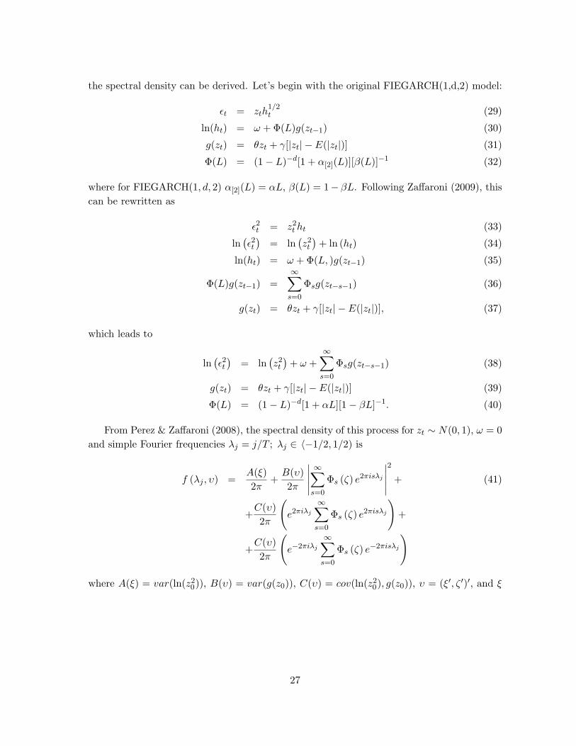
the spectral density can be derived. Let’s begin with the original FIEGARCH(1,d,2) model:

εt = zth1/2t (29)

ln(ht) = ω + Φ(L)g(zt−1) (30)

g(zt) = θzt + γ[|zt| − E(|zt|)] (31)

Φ(L) = (1− L)−d[1 + α[2](L)][β(L)]−1 (32)

where for FIEGARCH(1, d, 2) α[2](L) = αL, β(L) = 1− βL. Following Zaffaroni (2009), thiscan be rewritten as

ε2t = z2t ht (33)

ln(ε2t)

= ln(z2t

)+ ln (ht) (34)

ln(ht) = ω + Φ(L, )g(zt−1) (35)

Φ(L)g(zt−1) =∞∑s=0

Φsg(zt−s−1) (36)

g(zt) = θzt + γ[|zt| − E(|zt|)], (37)

which leads to

ln(ε2t)

= ln(z2t

)+ ω +

∞∑s=0

Φsg(zt−s−1) (38)

g(zt) = θzt + γ[|zt| − E(|zt|)] (39)

Φ(L) = (1− L)−d[1 + αL][1− βL]−1. (40)

From Perez & Zaffaroni (2008), the spectral density of this process for zt ∼ N(0, 1), ω = 0and simple Fourier frequencies λj = j/T ; λj ∈ 〈−1/2, 1/2) is

f (λj , υ) =A(ξ)2π

+B(υ)2π

∣∣∣∣∣∞∑s=0

Φs (ζ) e2πisλj

∣∣∣∣∣2

+ (41)

+C(υ)2π

(e2πiλj

∞∑s=0

Φs (ζ) e2πisλj

)+

+C(υ)2π

(e−2πiλj

∞∑s=0

Φs (ζ) e−2πisλj

)

where A(ξ) = var(ln(z20)), B(υ) = var(g(z0)), C(υ) = cov(ln(z2

0), g(z0)), υ = (ξ′, ζ ′)′, and ξ

27

is the vector of parameters in the distribution function of variable z. For zt ∼ N(0, 1):

A(ξ) = Ψ(12

) (42)

B(υ) = θ2 + δ2(1− µ2|z|) (43)

C(υ) = δµz(ψ(1)− ψ(12

)) (44)

µ|z| = E(|z|) =√

(2π

), (45)

where ψ(x) and Ψ(x) are digamma and trigamma functions respectively. Evaluated at Fourierfrequencies, this spectral density occurs in both terms of the FWE objective function. For ageneralization to zt following GED or Student-t distribution, see Perez & Zaffaroni (2008).

B Spectral Density Estimation

0 0.1 0.2 0.3 0.4 0.50

5

10

15

20

25

30

35

40

(a) d=0.25

0.1 0.2 0.3 0.4 0.5

10

20

30

40

50

60

70

80

90

100

(b) d=45

0 0.1 0.2 0.3 0.4 0.54

4.5

5

5.5

6

6.5

7

7.5

8

(c) d=-0.25

Figure 1: True spectral density

28

0 0.05 0.1 0.15 0.2 0.25

5

10

15

20

25

30

35

40

45

50

55

spectral density Fourier

spectral density true

spectral density Fourier averaged

spectral density approx

spectral density Wavelets

(a) d=0.25

0.05 0.1 0.15 0.2 0.250

20

40

60

80

100

120






(b) d=0.45

0 0.05 0.1 0.15 0.2 0.25

2

4

6

8

10

12

14






(c) d=-0.25

Figure 2: Spectral density estimation (d=0.25/0.45/-0.25), T=2048 (211), level=10, zoom29

C Partial Decomposition

0

1

2

3

4

5

6

A

B

C

D

E

F

(a)

0

5

10

15

20

25

30

35

A

B

C

D

E

F

G

H

(b)

Figure 3: Energy decomposition: Integrals of FIEGARCH spectral density over frequencyintervals respective to individual levels of decomposition, assuming various levels of longmemory (d=0.25, d=0.45, d=-0.25) and the coefficient sets from Table E.1 (a)

0

500

1000

1500

2000

2500

A

B

C

D

F

(a)

0

20000

40000

60000

80000

100000

120000

140000

160000

180000

200000

A

B

C

D

E

F

G

H

(b)

Figure 4: Energy decomposition: True variances of wavelet coefficients respective to individ-ual levels of decomposition and various levels of long memory (d=0.25, d=0.45, d=-0.25) andthe coefficient sets from Table E.1 (a)

30

(a) Coefficient Sets

Coefficients: d ω α β θ γ

A: 0.25 0 0.5 0.5 -0.3 0.5B: 0.45 0 0.5 0.5 -0.3 0.5C: -0.25 0 0.5 0.5 -0.3 0.5D: 0.25 0 0.9 0.9 -0.3 0.5E: 0.45 0 0.9 0.9 -0.3 0.5F: -0.25 0 0.9 0.9 -0.3 0.5G: 0.25 0 0.9 0.9 -0.9 0.9H: 0.45 0 0.9 0.9 -0.9 0.9

(b) Integrals over frequencies respective to levels for the coefficient sets from Tab.E.1(a)

A B C D E F G H

Level 1 1.1117 1.1220 1.0897 1.1505 1.1622 1.1207 1.1261 1.1399Level 2 0.5473 0.5219 0.6274 0.4776 0.4691 0.5306 0.6187 0.6058Level 3 0.3956 0.3693 0.4330 0.3246 0.3056 0.3959 1.1354 1.3453Level 4 0.3029 0.3341 0.2425 0.5559 0.7712 0.3528 2.9558 4.8197Level 5 0.2035 0.2828 0.1175 1.0905 2.1758 0.3003 6.0839 13.2127Level 6 0.1279 0.2297 0.0550 1.4685 3.9342 0.1965 8.2136 23.4144Level 7 0.0793 0.1883 0.0259 1.3523 4.7975 0.0961 7.6026 28.4723Level 8 0.0495 0.1584 0.0123 1.0274 4.8302 0.0408 5.8268 28.7771Level 9 0.0313 0.1368 0.0059 0.7327 4.5720 0.0169 4.1967 27.3822Level 10 0.0201 0.1206 0.0029 0.5141 4.2610 0.0071 2.9728 25.6404Level 11 0.0130 0.1080 0.0014 0.3597 3.9600 0.0030 2.0977 23.9192Level 12 0.0086 0.0979 0.0007 0.2518 3.6811 0.0013 1.4793 22.2986

(c) Sample Variances of DWT Wavelet Coefficients for the coefficient sets from Table E.1 (a)

A B C D E F G H

Level 1 4.4468 4.4880 4.3588 4.6020 4.6488 4.4828 4.5044 4,5596Level 2 4.3784 4.1752 5.0192 3.8208 3.7528 4.2448 4.9496 4.8464Level 3 6.3296 5.9088 6.9280 5.1936 4.8896 6.3344 18.1664 21.5248Level 4 9.6928 10.6912 7.7600 17.7888 24.6784 11.2896 94.5856 154.2304Level 5 13.0240 18.0992 7.5200 69.7920 139.2512 19.2192 389.3696 845.6128Level 6 16.3712 29.4016 7.0400 187.9680 503.5776 25.1520 1051.3408 2997.0432Level 7 20.3008 48.2048 6.6304 346.1888 1228.1600 24.6016 1946.2656 7288.9088Level 8 25.3440 81.1008 6.2976 526.0288 2473.0624 20.8896 2983.3216 14733,8752Level 9 32.0512 140.0832 6.0416 750.2848 4681.7280 17.3056 4297.4208 28039.3728Level 10 41.1648 246.9888 5.9392 1052.8768 8726.5280 14.5408 6088.2944 52511.5392Level 11 53.2480 442.3680 5.7344 1473.3312 16220.1600 12.2880 8592.1792 97973.0432Level 12 70.4512 801.9968 5.7344 2062.7456 30155.5712 10.6496 12118.4256 182670.1312

Table 1: Energy decomposition

31

D Convergence analysis

4 5

6 7

8 9

10 11

12 13

14

9 10 11 12 13 14

BIAS of d ( LA8, d=0,45)

0-0,025 -0,025-0 -0,05--0,025 -0,075--0,05

Sample length 2^(j), j = 9, 10, ...,14

Level of decomposition J = 4, 5, ..., 14

Legend

Plot name: Characteristic (BIAS) of estimates of

parameter (d) estimated by WWE with filter (LA8) given

true process specified by value of parameter d (d=0,45)

Characteristic (BIAS) for a specific sample length and level of decomposition is represented by a field 2x2, for level 4 by 2x1.

(1) Keeping the sample length constant, we see the effect of increasing the level of decomposition [estimation using increasing number of intervals respective to lower and lower frequencies]. At each level (j), N(j)=M/2^(j) coefficients is available, where M is the sample length.

(2) Keeping the level of decomposition constant, we see the effect of increasing the sample size [increasing the number of DWT coefficients available at each level (j): N(j)=M/2^(j)]. E.g. for two samples for which M*=2M, we have N(j)*=2N(j).

Figure 5: 3D Plots Guide

4 5

6 7

8 9

10 11

12 13

14

9 10

11 12

13 14

0,05-0,075

0,025-0,05

0-0,025

-0,025-0

-0,05--0,025

-0,075--0,05

-0,1--0,075

-0,125--0,1

-0,15--0,125

(a) Bias of d (LA8, d=0.25)

4 5

6 7

8 9

10 11

12 13

14

9 10

11 12

13 14

0-0,025

-0,025-0

-0,05--0,025

-0,075--0,05

-0,1--0,075

-0,125--0,1

-0,15--0,125

-0,175--0,15

-0,2--0,175

(b) Bias of d (LA8, d=0.45)

Figure 6: 3D Plots: Partial decomposition: d: Bias

32

4 5 6 7 8 9 10 11 12 13 14

0

0,05

0,1

0,15

0,2

0,25

0,3

9 10

11 12

13 14

0,25-0,3

0,2-0,25

0,15-0,2

0,1-0,15

0,05-0,1

0-0,05

(a) RMSE of d (LA8, d=0.25)

4 5 6 7 8 9 10 11 12 13 14

0

0,05

0,1

0,15

0,2

0,25

0,3

0,35

9 10

11 12

13 14

0,3-0,35

0,25-0,3

0,2-0,25

0,15-0,2

0,1-0,15

0,05-0,1

0-0,05

(b) RMSE of d (LA8, d=0.45)

Figure 7: 3D Plots: Partial decomposition: d: RMSE

4 5

6 7

8 9

10 11

12 13

14

9 10

11 12

13 14

0,05-0,075

0,025-0,05

0-0,025

-0,025-0

-0,05--0,025

-0,075--0,05

-0,1--0,075

-0,125--0,1

-0,15--0,125

(a) Bias of α (LA8, d=0.25)

4 5

6 7

8 9

10 11

12 13

14

9 10

11 12

13 14

0-0,025

-0,025-0

-0,05--0,025

-0,075--0,05

-0,1--0,075

-0,125--0,1

-0,15--0,125

-0,175--0,15

-0,2--0,175

(b) Bias of α (LA8, d=0.45)

Figure 8: 3D Plots: Partial decomposition: α: Bias

33

4 5 6 7 8 9 10 11 12 13 14

0

0,05

0,1

0,15

0,2

0,25

0,3

9 10

11 12

13 14

0,25-0,3

0,2-0,25

0,15-0,2

0,1-0,15

0,05-0,1

0-0,05

(a) RMSE of α (LA8, d=0.25)

4 5 6 7 8 9 10 11 12 13 14

0

0,05

0,1

0,15

0,2

0,25

0,3

0,35

9 10

11 12

13 14

0,3-0,35

0,25-0,3

0,2-0,25

0,15-0,2

0,1-0,15

0,05-0,1

0-0,05

(b) RMSE of α (LA8, d=0.45)

Figure 9: 3D Plots: Partial decomposition: α: RMSE

E Relative Performance

0 0.05 0.1 0.15 0.2 0.25 0.3 0.35 0.4 0.45 0.5

5

10

15

20

25

30

true spectral density

wavelets

Fourier

(a) T=512 (29), level=5(D4)

0 0.05 0.1 0.15 0.2 0.25 0.3 0.35 0.4 0.45 0.5

5

10

15

20

25

30

true spectral density

wavelets

Fourier

(b) T=2048 (211), level=5(D4)

Figure 10: Spectral density estimation: Wavelets (Level 5) vs Fourier

34

F Jumps: Features

0 200 400 600 800 1000 1200 1400 1600 1800 2000

-0.5

-0.4

-0.3

-0.2

-0.1

0

0.1

0.2

0.3

0.4

FIEGARCH(0.25,-7,0.5,0.5,-0.3,0.5), Jumps=[lambda=0.028, N(0,0.2)],filter=D4,transform=MODWT

True Data

True Jumps

(a) Effects of jumps in the time series

0 200 400 600 800 1000 1200 1400 1600 1800 2000

-0.6

-0.4

-0.2

0

0.2

0.4

FIEGARCH(0.25,-7,0.5,0.5,-0.3,0.5), Jumps=[lambda=0.028, N(0,0.2)],filter=D4,transform=MODWT

True Jumps

Correction

(b) Jump detection

Figure 11: Jumps in the data

0 100 200 300 400 500 600 700 800-20

-18

-16

-14

-12

-10

-8

-6

-4

-2

0FIEGARCH(0.25,-7,0.5,0.5,-0.3,0.5);Jumps[lambda=0.028; N(0,0.2)]

ln(Y2) True

ln(Y2) No Jumps

Jump locations (-1)

(a) lambda=0.028; N(0,0.2)

200 400 600 800 1000 1200 1400 1600 1800 2000

-20

-15

-10

-5

0

FIEGARCH(0.25,-7,0.5,0.5,-0.3,0.5);Jumps[lambda=0.007; N(0,3)]

ln(Y2) True

ln(Y2) No Jumps

Jump locations (-1)

(b) Stronger jumps: lambda=0.007; N(0,3)

Figure 12: Jumps after transformation ln(y2)

G Jumps: Results

35

No

Jum

ps;

N=

2048

No

Jum

ps;

N=

16384

No

Jum

ps;

N=

2048

PA

RT

RU

EM

ET

HO

DM

EA

NB

IAS

RM

SE

ME

AN

BIA

SR

MSE

PA

RM

EA

NB

IAS

RM

SE

d0.2

50

WW

EM

OD

WT

0.1

65

-0.0

85

0.2

25

0.2

53

0.0

03

0.0

42

0.4

50

0.3

62

-0.0

88

0.1

70

WW

EM

OD

WT

20.1

68

-0.0

82

0.2

27

--

--

--

FW

E0.2

12

-0.0

38

0.1

47

0.2

51

0.0

01

0.0

36

0.4

15

-0.0

35

0.0

87

FW

E2

0.2

13

-0.0

37

0.1

46

--

--

--

ML

E0.2

20

-0.0

30

0.0

85

--

-0.4

33

-0.0

17

0.0

43

ML

E2

0.2

28

-0.0

22

0.0

86

--

--

--

ω-7

.000

ML

E-7

.076

-0.0

76

0.1

74

--

--7

.458

-0.4

58

0.7

39

ML

E2

-7.0

83

-0.0

83

0.1

82

--

--

--

OT

HE

R-7

.002

-0.0

02

0.1

97

-7.0

03

-0.0

03

0.0

74

-6.9

99

0.0

01

0.6

96

OT

HE

R2

-7.0

15

-0.0

15

0.1

98

--

--

--

α2

0.5

00

WW

EM

OD

WT

0.4

34

-0.0

66

0.3

49

0.3

28

-0.1

72

0.2

29

0.3

24

-0.1

76

0.3

95

WW

EM

OD

WT

20.4

26

-0.0

74

0.3

58

--

--

--

FW

E0.5

27

0.0

27

0.3

43

0.5

12

0.0

12

0.1

68

0.4

75

-0.0

25

0.3

48

FW

E2

0.5

21

0.0

21

0.3

33

--

--

--

ML

E0.5

03

0.0

03

0.1

21

--

-0.4

87

-0.0

13

0.1

28

ML

E2

0.4

64

-0.0

36

0.1

36

--

--

--

β1

0.5

00

WW

EM

OD

WT

0.5

59

0.0

59

0.2

49

0.5

23

0.0

23

0.0

78

0.6

10

0.1

10

0.1

78

WW

EM

OD

WT

20.5

61

0.0

61

0.2

53

--

--

--

FW

E0.5

20

0.0

20

0.1

99

0.4

99

-0.0

01

0.0

65

0.5

54

0.0

54

0.1

35

FW

E2

0.5

17

0.0

17

0.2

14

--

--

--

ML

E0.5

29

0.0

29

0.1

01

--

-0.5

27

0.0

27

0.0

63

ML

E2

0.5

37

0.0

37

0.1

09

--

--

--

θ-0

.300

WW

EM

OD

WT

-0.2

83

0.0

17

0.1

80

-0.3

37

-0.0

37

0.0

78

-0.3

14

-0.0

14

0.1

46

WW

EM

OD

WT

2-0

.261

0.0

39

0.1

82

--

--

--

FW

E-0

.244

0.0

56

0.1

82

-0.2

79

0.0

21

0.0

77

-0.2

42

0.0

58

0.1

58

FW

E2

-0.2

22

0.0

78

0.1

89

--

--

--

ML

E-0

.301

-0.0

01

0.0

26

--

--0

.301

-0.0

01

0.0

24

ML

E2

-0.2

82

0.0

18

0.0

31

--

--

--

γ0.5

00

WW

EM

OD

WT

0.4

81

-0.0

19

0.1

96

0.4

89

-0.0

11

0.0

85

0.5

04

0.0

04

0.2

18

WW

EM

OD

WT

20.4

72

-0.0

28

0.1

93

--

--

--

FW

E0.5

09

0.0

09

0.1

75

0.5

04

0.0

04

0.0

83

0.5

26

0.0

26

0.2

02

FW

E2

0.4

97

-0.0

03

0.1

74

--

--

--

ML

E0.4

99

-0.0

01

0.0

45

--

-0.5

07

0.0

07

0.0

44

ML

E2

0.4

91

-0.0

09

0.0

48

--

--

--

Tab

le2:

Mon

teC

arlo

No

Jum

ps:

d=0.

25/0

.45;

ML

E,F

WE

,MO

DW

T(D

4),2

:C

orre

cted

usin

gD

onoh

oan

dJo

hnst

one

thre

shol

d

36

Jum

p[0

.028,N

(0,0

.2)]

;N=

2048

Jum

p[0

.028,N

(0,0

.2)]

;N=

16384

Jum

p[0

.028,N

(0,0

.2)]

;N=

2048

PA

RT

RU

EM

ET

HO

DM

EA

NB

IAS

RM

SE

ME

AN

BIA

SR

MSE

PA

RM

EA

NB

IAS

RM

SE

d0.2

50

WW

EM

OD

WT

0.1

45

-0.1

05

0.2

14

--

-0.4

50

--

-W

WE

MO

DW

T2

0.1

54

-0.0

96

0.2

25

0.2

35

-0.0

15

0.0

42

0.3

47

-0.1

03

0.1

79

FW

E0.1

95

-0.0

55

0.1

42

--

--

--

FW

E2

0.2

06

-0.0

44

0.1

43

0.2

31

-0.0

19

0.0

38

0.4

03

-0.0

47

0.0

91

ML

E0.0

18

-0.2

32

0.3

53

--

--

--

ML

E2

0.0

99

-0.1

51

0.2

51

--

-0.1

87

-0.2

63

0.3

14

ω-7

.000

ML

E-5

.662

1.3

38

1.4

50

--

--

--

ML

E2

-6.2

82

0.7

18

0.8

01

--

--5

.529

1.4

71

1.6

62

OT

HE

R-6

.887

0.1

13

0.2

21

--

--

--

OT

HE

R2

-6.9

42

0.0

58

0.2

03

-6.9

41

0.0

59

0.0

96

-6.9

46

0.0

54

0.6

77

α2

0.5

00

WW

EM

OD

WT

0.4

75

-0.0

25

0.4

37

--

--

--

WW

EM

OD

WT

20.4

92

-0.0

08

0.4

02

0.5

57

0.0

57

0.2

43

0.3

90

-0.1

10

0.4

47

FW

E0.5

61

0.0

61

0.4

54

--

--

--

FW

E2

0.5

82

0.0

82

0.4

00

0.7

31

0.2

31

0.2

97

0.5

35

0.0

35

0.4

28

ML

E0.6

67

0.1

67

0.3

85

--

--

--

ML

E2

0.6

52

0.1

52

0.2

87

--

-0.6

05

0.1

05

0.3

08

β1

0.5

00

WW

EM

OD

WT

0.5

92

0.0

92

0.2

90

--

--

--

WW

EM

OD

WT

20.5

78

0.0

78

0.2

64

0.5

35

0.0

35

0.0

87

0.6

36

0.1

36

0.2

03

FW

E0.5

46

0.0

46

0.2

66

--

--

--

FW

E2

0.5

29

0.0

29

0.2

31

0.5

19

0.0

19

0.0

68

0.5

79

0.0

79

0.1

64

ML

E0.4

06

-0.0

94

0.4

52

--

--

--

ML

E2

0.5

03

0.0

03

0.2

50

--

-0.6

19

0.1

19

0.2

40

θ-0

.300

WW

EM

OD

WT

-0.4

91

-0.1

91

0.2

72

--

--

--

WW

EM

OD

WT

2-0

.385

-0.0

85

0.1

89

-0.3

98

-0.0

98

0.1

08

-0.3

84

-0.0

84

0.1

74

FW

E-0

.455

-0.1

55

0.2

46

--

--

--

FW

E2

-0.3

48

-0.0

48

0.1

75

-0.3

56

-0.0

56

0.0

65

-0.3

24

-0.0

24

0.1

53

ML

E-0

.214

0.0

86

0.1

30

--

--

--

ML

E2

-0.2

11

0.0

89

0.1

04

--

--0

.176

0.1

24

0.1

37

γ0.5

00

WW

EM

OD

WT

0.2

03

-0.2

97

0.3

65

--

--

--

WW

EM

OD

WT

20.3

22

-0.1

78

0.2

71

0.2

87

-0.2

13

0.2

31

0.2

76

-0.2

24

0.3

22

FW

E0.2

57

-0.2

43

0.3

15

--

--

--

FW

E2

0.3

65

-0.1

35

0.2

31

0.3

13

-0.1

87

0.2

02

0.3

17

-0.1

83

0.2

91

ML

E0.2

87

-0.2

13

0.2

56

--

--

--

ML

E2

0.3

40

-0.1

60

0.1

80

--

-0.3

47

-0.1

53

0.1

79

Tab

le3:

Mon

teC

arlo

Jum

ps:d

=0.

25/0.

45;

Poi

sson

lam

bda

=0.

028;N

(0;0.2

);F

WE

,M

OD

WT

(D4)

,2:

Cor

rect

edus

ing

Don

oho

and

John

ston

eth

resh

old

37

Main

Sta

tsM

AD

quanti

les

Cat

ME

TH

OD

ME

AN

ER

RM

AD

RM

SE

0.5

00.9

00.9

50.9

9

inW

WE

MO

DW

T6.1

308e-

05

0.0

0039032

0.0

052969

--

--

WW

EM

OD

WT

22.2

383e-

05

0.0

0040778

0.0

034541

--

--

WW

ED

WT

8.3

135e-

05

0.0

0044932

0.0

11577

--

--

WW

ED

WT

22.3

63e-

05

0.0

0043981

0.0

050438

--

--

FW

E5.9

078e-

05

0.0

0037064

0.0

0087854

--

--

FW

E2

1.4

242e-

05

0.0

0038604

0.0

011961

--

--

ML

E6.0

381e-

06

9.3

694e-

05

0.0

0019804

--

--

ML

E2

-3.3

242e-

05

0.0

0011734

0.0

0028776

--

--

out

WW

EM

OD

WT

105.3

851

105.3

856

3277.1

207

0.0

0015361

0.0

010525

0.0

019431

0.0

060853

WW

EM

OD

WT

2-7

.6112e-

05

0.0

0058276

0.0

020436

0.0

0016482

0.0

010512

0.0

020531

0.0

072711

WW

ED

WT

0.0

0013817

0.0

0066928

0.0

031579

0.0

0017219

0.0

012156

0.0

020541

0.0

065611

WW

ED

WT

20.0

0087082

0.0

015663

0.0

27558

0.0

0017181

0.0

012497

0.0

022271

0.0

072191

FW

E2.9

498e-

05

0.0

0050763

0.0

015745

0.0

0014566

0.0

010839

0.0

018926

0.0

05531

FW

E2

0.0

0038499

0.0

010395

0.0

14191

0.0

0015425

0.0

011351

0.0

01989

0.0

081017

ML

E-1

.5041e-

06

0.0

0012211

0.0

0035147

4.0

442e-

05

0.0

0024483

0.0

0043587

0.0

01595

ML

E2

-0.0

0010455

0.0

0024125

0.0

015605

4.3

599e-

05

0.0

0030553

0.0

0063378

0.0

038043

Err

or

quanti

les

AE

rror

quanti

les

B

0.0

10.0

50.1

00.9

00.9

50.9

9

out

WW

EM

OD

WT

-0.0

033827

-0.0

010722

-0.0

004865

0.0

0063385

0.0

010345

0.0

048495

WW

EM

OD

WT

2-0

.0045312

-0.0

013419

-0.0

0062698

0.0

0053531

0.0

0089684

0.0

051791

WW

ED

WT

-0.0

040691

-0.0

01223

-0.0

0059588

0.0

0065501

0.0

012118

0.0

04838

WW

ED

WT

2-0

.003994

-0.0

013952

-0.0

0071166

0.0

0059679

0.0

010616

0.0

050457

FW

E-0

.0035752

-0.0

010712

-0.0

0053169

0.0

0061822

0.0

01086

0.0

04636

FW

E2

-0.0

042148

-0.0

0129

-0.0

0063194

0.0

005657

0.0

010577

0.0

048622

ML

E-0

.00079412

-0.0

0024382

-0.0

0013312

0.0

0010297

0.0

0026481

0.0

013195

ML

E2

-0.0

019587

-0.0

0046351

-0.0

0021734

7.5

622e-

05

0.0

0018216

0.0

0077541

Not

Corr

ecte

d:M

ean

of

N-n

ext

true

valu

esto

be

fore

cast

ed:

0.0

016845;

Tota

lva

lid=

967,

i.e.

96.7

%of

Mfa

ils-

ML

E=

0%

,fa

ils-

FW

E=

0.8

%,

fails-

MO

DW

T=

2.1

%,

fails-

DW

T=

1.5

%C

orr

ecte

d:

Mea

nof

N-n

ext

true

valu

esto

be

fore

cast

ed:

0.0

016852

;T

ota

lva

lid=

959,

i.e.

95.9

%of

Mfa

ils-

ML

E=

0%

,fa

ils-

FW

E=

1.3

%,

fails-

MO

DW

T=

1.7

%,

fails-

DW

T=

2.7

%

Tab

le4:

Fore

cast

ing:

N=

2048

;N

oJu

mps

;M

LE

,F

WE

,MO

DW

T(D

4),D

WT

(D4)

,2:

Cor

rect

edus

ing

Don

oho

and

John

ston

eth

resh

old

38

Main

Sta

tsM

AD

quanti

les

Cat

ME

TH

OD

ME

AN

ER

RM

AD

RM

SE

0.5

00.9

00.9

50.9

9

inW

WE

MO

DW

T7.5

22e-

06

0.0

0015889

0.0

0032423

--

--

WW

ED

WT

8.5

378e-

06

0.0

0017736

0.0

0038026

--

--

FW

E6.3

006e-

06

0.0

0014367

0.0

0032474

--

--

ML

E-

--

--

--

out

WW

EM

OD

WT

9.3

951e-

06

0.0

0018394

0.0

0054618

7.1

556e-

05

0.0

0040438

0.0

007369

0.0

015565

WW

ED

WT

2.1

579e-

05

0.0

002107

0.0

0084705

7.1

483e-

05

0.0

0041876

0.0

0074376

0.0

018066

FW

E-3

.3569e-

06

0.0

0017794

0.0

0067805

5.6

684e-

05

0.0

0035132

0.0

005922

0.0

01811

ML

E-

--

--

--

Err

or

quanti

les

AE

rror

quanti

les

B

0.0

10.0

50.1

00.9

00.9

50.9

9

out

WW

EM

OD

WT

-0.0

011566

-0.0

0040454

-0.0

0021569

0.0

0021003

0.0

004025

0.0

013515

WW

ED

WT

-0.0

011033

-0.0

0038209

-0.0

0018247

0.0

0023587

0.0

0049025

0.0

016387

FW

E-0

.00087002

-0.0

0034408

-0.0

0018571

0.0

0018593

0.0

0035741

0.0

010787

ML

E-

--

--

-

Not

Corr

ecte

d:M

ean

of

N-n

ext

true

valu

esto

be

fore

cast

ed:

0.0

015516;

Tota

lva

lid=

1000,

i.e.

100

%of

Mfa

ils-

ML

E=

0%

,fa

ils-

FW

E=

0%

,fa

ils-

MO

DW

T=

0%

,fa

ils-

DW

T=

0%

Tab

le5:

Fore

cast

ing:

N=

1638

4;N

oJu

mps

;M

LE

,F

WE

,MO

DW

T(D

4),D

WT

(D4)

,2:

Cor

rect

edus

ing

Don

oho

and

John

ston

eth

resh

old

39

Main

Sta

tsM

AD

quanti

les

Cat

ME

TH

OD

ME

AN

ER

RM

AD

RM

SE

0.5

00.9

00.9

50.9

9

inW

WE

MO

DW

T0.0

0026281

0.0

010841

0.0

2023

--

--

WW

ED

WT

0.0

0022639

0.0

011206

0.0

13151

--

--

FW

E0.0

0027127

0.0

010458

0.0

05243

--

--

ML

E5.7

279e-

05

0.0

0026995

0.0

012167

--

--

out

WW

EM

OD

WT

Inf

Inf

Inf

0.0

0016653

0.0

024597

0.0

05308

0.0

40031

WW

ED

WT

924.8

354

924.8

375

28648.7

373

0.0

0017788

0.0

024428

0.0

049679

0.0

40403

FW

E-0

.00010684

0.0

015807

0.0

078118

0.0

0016022

0.0

025471

0.0

057388

0.0

31548

ML

E0.0

002289

0.0

004843

0.0

039972

4.2

589e-

05

0.0

0052307

0.0

010187

0.0

078509

Err

or

quanti

les

AE

rror

quanti

les

B

0.0

10.0

50.1

00.9

00.9

50.9

9

out

WW

EM

OD

WT

-0.0

13427

-0.0

024269

-0.0

0087296

0.0

010521

0.0

026019

0.0

13128

WW

ED

WT

-0.0

13075

-0.0

025811

-0.0

010018

0.0

0089545

0.0

023095

0.0

165

FW

E-0

.012356

-0.0

02209

-0.0

0081063

0.0

010042

0.0

02777

0.0

14773

ML

E-0

.0016025

-0.0

0044789

-0.0

002568

0.0

0017179

0.0

0056713

0.0

051968

Not

Corr

ecte

d:M

ean

of

N-n

ext

true

valu

esto

be

fore

cast

ed:

0.0

064152;

Tota

lva

lid=

962,

i.e.

96.2

%of

Mfa

ils-

ML

E=

0%

,fa

ils-

FW

E=

1%

,fa

ils-

MO

DW

T=

1.9

%,

fails-

DW

T=

2.1

%

Tab

le6:

Fore

cast

ing:

N=

2048

;d=

0.45

;N

oJu

mps

;M

LE

,F

WE

,MO

DW

T(D

4),D

WT

(D4)

,2:

Cor

rect

edus

ing

Don

oho

and

John

ston

eth

resh

old

40

Main

Sta

tsM

AD

quanti

les

Cat

ME

TH

OD

ME

AN

ER

RM

AD

RM

SE

0.5

00.9

00.9

50.9

9

inW

WE

MO

DW

T0.0

024292

0.0

027027

0.0

31109

--

--

WW

EM

OD

WT

20.0

0049847

0.0

0088238

0.0

10266

WW

ED

WT

0.0

022873

0.0

025833

0.0

29094

--

--

WW

ED

WT

20.0

0051788

0.0

0092081

0.0

13946

FW

E0.0

024241

0.0

026398

0.0

30474

--

--

FW

E2

0.0

0046896

0.0

0080786

0.0

1562

ML

E0.0

0099962

0.0

013136

0.0

022127

--

--

ML

E2

0.0

0021708

0.0

005767

0.0

011708

out

WW

EM

OD

WT

Inf

Inf

Inf

0.0

0027911

0.0

019584

0.0

043937

0.0

74726

WW

EM

OD

WT

212837.4

644

12837.4

647

361761.8

976

0.0

0020755

0.0

012984

0.0

021954

0.0

64956

WW

ED

WT

0.0

10776

0.0

10967

0.1

4233

0.0

0032328

0.0

020108

0.0

048951

0.0

86811

WW

ED

WT

2In

fIn

fIn

f0.0

0019516

0.0

013594

0.0

02609

0.0

8235

FW

E0.0

098899

0.0

10026

0.1

5737

0.0

0025416

0.0

019525

0.0

047286

0.0

73048

FW

E2

1.4

046

1.4

048

36.7

106

0.0

0017622

0.0

012063

0.0

024169

0.0

57823

ML

E0.0

014788

0.0

017573

0.0

066777

0.0

0099906

0.0

01951

0.0

027302

0.0

19721

ML

E2

0.0

022114

0.0

025386

0.0

53463

0.0

0034636

0.0

0094187

0.0

016393

0.0

082677

Err

or

quanti

les

AE

rror

quanti

les

B

0.0

10.0

50.1

00.9

00.9

50.9

9

out

WW

EM

OD

WT

-0.0

014262

-0.0

0061569

-0.0

0023517

0.0

018119

0.0

043937

0.0

74726

WW

EM

OD

WT

2-0

.002004

-0.0

007648

-0.0

0033609

0.0

010397

0.0

018978

0.0

64956

WW

ED

WT

-0.0

014902

-0.0

0065937

-0.0

0028371

0.0

018904

0.0

048951

0.0

86811

WW

ED

WT

2-0

.002635

-0.0

0076962

-0.0

0031466

0.0

0099973

0.0

020434

0.0

8235

FW

E-0

.00097176

-0.0

0039409

-0.0

0021056

0.0

019269

0.0

047286

0.0

73048

FW

E2

-0.0

019851

-0.0

0057545

-0.0

0025878

0.0

0087435

0.0

020268

0.0

57823

ML

E-0

.0033888

-0.0

004285

0.0

0016064

0.0

018323

0.0

023536

0.0

19688

ML

E2

-0.0

030739

-0.0

0075814

-0.0

0029836

0.0

0066214

0.0

0099507

0.0

059062

Corr

ecte

d:

Mea

nof

N-n

ext

true

valu

esto

be

fore

cast

ed:

0.0

01324;

Tota

lva

lid=

801,

i.e.

80.1

%of

Mfa

ils-

ML

E=

0%

,fa

ils-

FW

E=

7%

,fa

ils-

MO

DW

T=

13.4

%,

fails-

DW

T=

12.5

%N

ot

Corr

ecte

d:

Mea

nof

N-n

ext

true

valu

esto

be

fore

cast

ed:

0.0

01324;

Tota

lva

lid=

45.1

,i.e.

%of

Mfa

ils-

ML

E=

0%

,fa

ils-

FW

E=

35.2

%,

fails-

MO

DW

T=

43.4

%,

fails-

DW

T=

41.6

%

Tab

le7:

Fore

cast

ing:

N=

2048

;Ju

mps

Lam

bda=

0.02

8,N

(0,

0.2)

;M

LE

,F

WE

,MO

DW

T(D

4),D

WT

(D4)

,2:

Cor

rect

edus

ing

Don

oho

and

John

ston

eth

resh

old

41

Main

Sta

tsM

AD

quanti

les

Cat

ME

TH

OD

ME

AN

ER

RM

AD

RM

SE

0.5

00.9

00.9

50.9

9

inW

WE

MO

DW

T0.0

0079621

0.0

010536

0.0

19562

--

--

WW

ED

WT

0.0

0074677

0.0

010165

0.0

18346

--

--

FW

E0.0

0052705

0.0

0074759

0.0

094745

--

--

ML

E-

--

--

--

out

WW

EM

OD

WT

Inf

Inf

Inf

0.0

002394

0.0

015

0.0

037696

0.0

88609

WW

ED

WT

Inf

Inf

Inf

0.0

0022172

0.0

016482

0.0

039952

0.0

43464

FW

E0.0

10034

0.0

10249

0.2

3919

0.0

0017951

0.0

014685

0.0

037604

0.0

4528

ML

E-

--

--

--

Err

or

quanti

les

AE

rror

quanti

les

B

0.0

10.0

50.1

00.9

00.9

50.9

9

out

WW

EM

OD

WT

-0.0

025009

-0.0

006746

-0.0

0028513

0.0

011776

0.0

033089

0.0

88609

WW

ED

WT

-0.0

025573

-0.0

0057909

-0.0

0028814

0.0

012299

0.0

033547

0.0

43464

FW

E-0

.0018013

-0.0

0048645

-0.0

0022585

0.0

011465

0.0

030639

0.0

4528

ML

E-

--

--

-

Corr

ecte

d:M

ean

of

N-n

ext

true

valu

esto

be

fore

cast

ed:

0.0

016747;

Tota

lva

lid=

948,

i.e.

94.8

%of

Mfa

ils-

ML

E=

-%

,fa

ils-

FW

E=

0.4

%,

fails-

MO

DW

T=

3.1

%,

fails-

DW

T=

2.5

%

Tab

le8:

Fore

cast

ing:

N=

1638

4;Ju

mps

Lam

bda=

0.02

8,N

(0,

0.2)

;M

LE

,F

WE

,MO

DW

T(D

4),D

WT

(D4)

,2:

Cor

rect

edus

ing

Don

oho

and

John

ston

eth

resh

old

42

IES Working Paper Series

2014 1. Diana Zigraiova, Petr Jakubik: Systemic Event Prediction by Early Warning System

2. Pavla Blahova, Karel Janda, Ladislav Kristoufek: The Perspectives for Genetically Modified Cellulosic Ethanol in the Czech Republic

3. Oxana Babecká Kucharčuková: The impact of exchange rate volatility on trade: Evidence for the Czech Republic

4. Oliver Polyák: The Impact of Euro Adoption on Export Performance: Comparison of the Czech Republic and Slovakia

5. Lucie Davidová, Vladimír Benáček: Determinants of Austrian International Trade:

Analysis Based on the Gravity Model

6. Julie Chytilová, Václav Korbel: Individual and Group Cheating Behavior: A Field Experiment with Adolescents

7. Petr Janský: Consumer Demand System Estimation and Value Added Tax Reforms in the Czech Republic

8. Pavel Hait, Petr Janský: Inflation Differentials among Czech Households

9. Hana Džmuráňová, Petr Teplý: Risk management of savings accounts

10. Tomáš Fiala, Tomáš Havránek: Ailing Mothers, Healthy Daughters? Contagion in the Central European Banking Sector

11. Petra Andrlíková: Is Barrier version of Merton model more realistic? Evidence from Europe

12. Martin Pospíšil, Jiří Schwarz: Bankruptcy, Investment, and Financial Constraints:

Evidence from a Post-Transition Economy

13. Matt Hunt, Goran Serdarević, Tom Ovington, Clive Kenny: Evidence for a ladder of investment in Central and Eastern European countries

14. Petra Andrlíková: Bayesian default probability models

15. Petra Buzková: Has the Relationship Between Market and Model CDS Price Changed

during the EMU Debt Crisis?

16. Jakub Černý, Jiří Witzany: Interest Rate Swap Credit Valuation Adjustment

17. Martin Gregor: Receiver's access fee for a single sender

18. Pavel Ryska: Deflation and Economic Growth in Long-Term Perspective

19. Michal Paulus, Eva Michalíková, Vladimír Benáček: German International Trade:

Interpreting Export Flows According to the Gravity Model 20. Michal Bauer, Nathan Fiala, Ian Levely: Trusting Former Rebels: An Experimental

Approach to Understanding Reintegration after Civil War

21. Michal Skořepa: Family Matters: Concurrent Capital Buffers in a Banking Group

22. Martin Gregor: Access Fees for Competing Lobbies

23. Jozef Baruník, František Čech: On the Modelling and Forecasting Multivariate Realized Volatility: Generalized Heterogeneous Autoregressivee (GHAR) Model

24. Roman Horváth, Ayaz Zeynalov: The Natural Resource Curse and Institutions in Post-Soviet Countries

25. Petr Janský: Impact of Excise Duties on Households in the Czech Republic

26. Petr Jakubík, Thomas Reininger: What Are the Key Determinants of Nonperforming

Loans in CESEE?

27. Jaromír Baxa, Tomáš Olešňaník: Current Accounts in the Eurozone Countries: The Role

of Euro, Fiscal Policies and Financial Developments

28. Petr Polák: The Productivity Paradox: A Meta-analysis

29. Tomáš Havránek, Zuzana Iršová, Karel Janda, David Zilberman: Selective Reporting and the Social Cost of Carbon

30. Jozef Baruník, Tomáš Křehlík: Coupling High-Frequency Data with Nonlinear Models in

Multiple-Step-ahead Forecasting of Energy Markets‘ Volatility

31. Lenka Šťastná, Jana Votápková: Efficiency of Hospitals in the Czech Republic: Conditional Efficiency Approach

32. Eva Michalíková, Michal Paulus: Gravity Model Analysis: Robust Evidence from the Czech Republic and Corruption Matching

33. Jozef Baruník, Lucie Kraicová: Estimation of Long Memory in Volatility Using Wavelets

All papers can be downloaded at: http://ies.fsv.cuni.cz

Univerzita Karlova v Praze, Fakulta sociálních věd

Institut ekonomických studií [UK FSV – IES] Praha 1, Opletalova 26

E-mail : [email protected] http://ies.fsv.cuni.cz



estimation of long memory in volatility using wavelets

Documents