Wavelet Methods in Seismology:application of wavelets to multiscaleanalysis and non-linear estimation

Felix Herrmann ERL-MIT

February 17, 2002

References

Some useful references: [1, 2, 5, 14, 9, 6, 13]

Objective: Obtain information on reservoir properties

from seismic data (indirect measurements).

Method: Send waves in the earth and measure the

response.

Physics: Elastodynamic wave equation (hyperbolic

PDE).

Math: Linearized inverse scattering problem.

Stat.: Estimation problem (noise in measurements)

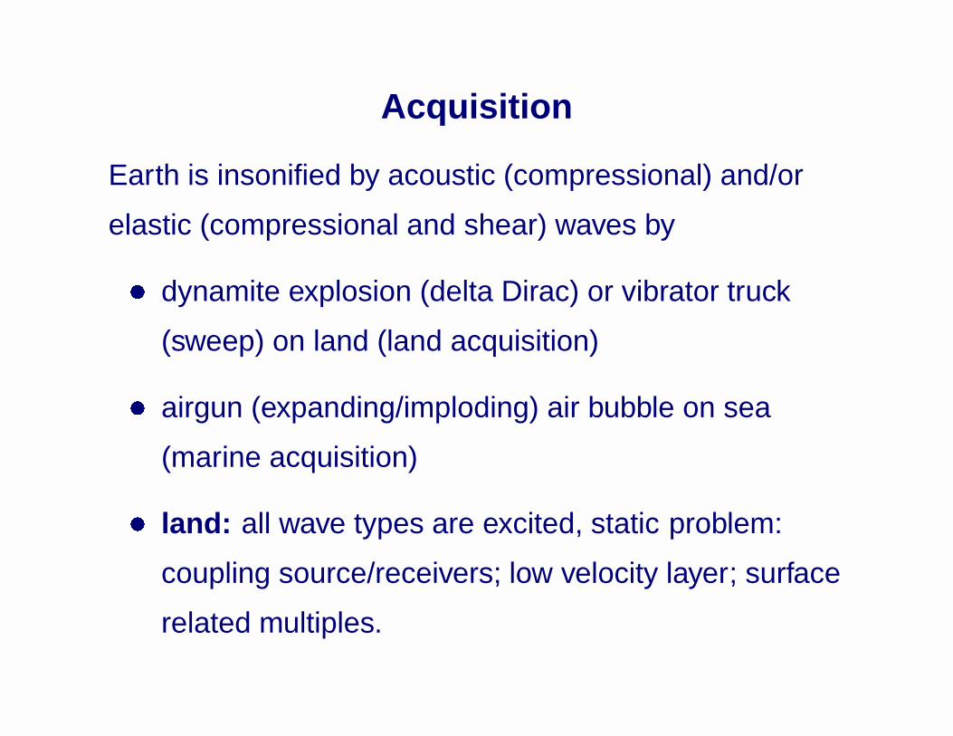
Acquisition

Earth is insonified by acoustic (compressional) and/or

elastic (compressional and shear) waves by

� dynamite explosion (delta Dirac) or vibrator truck

(sweep) on land (land acquisition)

� airgun (expanding/imploding) air bubble on sea

(marine acquisition)

� land: all wave types are excited, static problem:

coupling source/receivers; low velocity layer; surface

related multiples.

� marine: only compresssional waves are excited,

“static” problem: surface and water column related

multiples; coupling with the sea bottom.

Acquisition� On land data is acquired by geophones on a line

with spacing of �25m and length of kilometers.

� At sea data is acquired by hydrophones on a line.

Data are bandwidth limited both in space and time.

Temporal frequency range is �10 � � � 100Hz, vertical

wavelength 50 � � � 200m.

Data are aperture limited (finite cable length).

Acquisition setup

hydrophone airgun

geophone

source

well log

∆ ∆ ∆ ∆∆∆∆∆∆∆∆

Pre-Processed Marine data

0

1

2

3

4

time [

s]

-3000 -2000 -1000offset [m]

Well-log data

2300

2400

2500

2600

2700

2800

2900

3000

3100

32002000 3000 4000 5000 6000

2400

2450

2500

2550

2600

2650

2700

2000 3000 4000 5000 6000

dept

h[ m

]

p-wave velocity [ms�1]

dept

h[ m

]

p-wave velocity [ms�1]

Physical model

Acoustic/elastic scalar/vector waves are described by the wave

equation:

(A �t u) = f

� u is a space-time parametrized actual field vector.

� f is a space-time parametrized initial source field vector.

� A �t � is infinitesimal operator linking changes in u to the

source field f .

� �t possible non-local time behavior (via convolution),

i.e. dispersion/relaxation.

Post-stack migration example

−100

−50

0

50

100

trace #

time

original data

100 200 300 400 500 600 700 800

100

200

300

400

500

600

700

800

900

1000

Pre-stack migrated gather

Imaged pre−stack reflectivity

time

p−400 −300 −200 −100 0 100 200 300 400

0

0.5

1

1.5

2

2.5

Physical model

Acoustic/elastic scalar/vector waves are described by

(A �t u) = f

� u is the space-time actual field vector.

� f is the space-time initial source field vector.

� A �t � is infinitesimal operator linking changes in u

to the source field f .

� �t possible non-local time behavior (via

convolution), i.e. dispersion/relaxation.

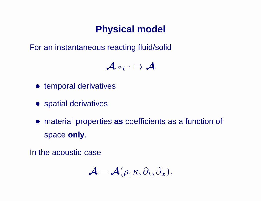
Physical model

For an instantaneous reacting fluid/solid

A �t � 7! A

� temporal derivatives

� spatial derivatives

� material properties as coefficients as a function of

space only.

In the acoustic case

A = A(�; �; @t; @x):

Physical model

The wave equation is

� given by a second order hyperbolic PDE.

� linear in field quantities and time (one temporal

frequency the same one out).

� non-linear in the coefficients.

“Describes” the forward and inverse problems, i.e.

�; �; f ! u

u; f ! �; �:

Physical model

Naive solution

inf�;�;fku� ~uk

in some norm.

1. inverse problem is ill-posed:

� limited aperture

� dispersion

� bandwidth limitation

2. dynamics of the forward problem not well

understood.

Linearized Scattering problem

Forward problem [4, 3, 7, 8]:

y = Kx

where

y = measured data.

K = linear scat. oper. () (generalized) Radon.

x = medium perturbation.

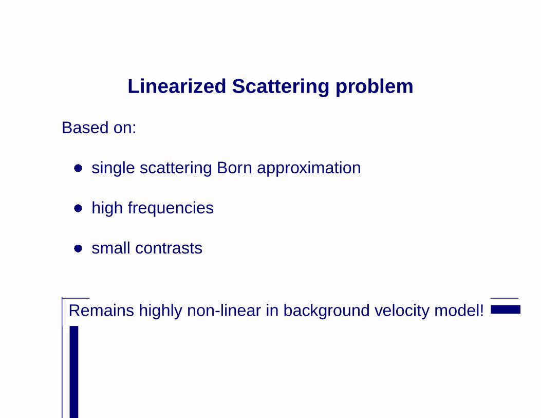
Linearized Scattering problem

Based on:

� single scattering Born approximation

� high frequencies

� small contrasts

Remains highly non-linear in background velocity model!

Uncertainty

Data:

y = Kx+ n

where

y = measured data.

K = linear scat. oper. () (generalized) Radon.

x = medium perturbation.

n = noise.

Imaging and Inversion

More or less noise free:

^x = (K�

K)�1

| {z }

Inversion

Migration

z}|{

K

�

y

where

K

� = adjoint adjoint () inverse Radon.

K

�

K = Normal/Gram operator.

(K�

K)�1 = compensation amplitude effects.

Linearized inverse scattering

In the abscence of caustics [4, 3]:

� K

�

K is DE.

� K

�

K is diagonal.

� preserves singularities in x.

For media with caustics [7, 8]:

� Maslov.

� micro-local.

Aim of this course

1. analyze x from y via K�

y:� detect and characterize singularities localy =)

Holder regularity.

� detect and characterize singularities globally =)

multifractal singularity spectrum.

2. non-linearly estimate x from K

�

y with y noisy:

� without a lot of a priory information.

� deal with non-stationarity.

� use basis functions and non-linear thresholding.

Wavelets

Why wavelets?

� they are related to DE-operators.

� allow for microlocal analysis of singularities [11, 12].

� (generalized) convolution model is related to the

continuous wavelet transform (CWT) at one scale

[7, 10].

� seismic waves detect singularities.

Sedimentary Records and Seismic

Reflectivity

500 1000 1500 2000 2500 3000 3500−200

0200

T1

X1

Y1

T2

X2

Y2

500 1000 1500 2000 2500 3000 3500

0

50

100

150

200

250

500 1000 1500 2000 2500 3000 35000

20004000

T3

X3

Y3

Wavelets versus Seismic Waves

Forward map:y(r; s; t) = Kf�c;x; 'g(r; s; t) = Kx:

1-D homogeneous background model:

p(p; z = 0; t) =

�M(p)

�2�q(p)Wfx; g(

�2�q(p);

t

2�q(p));

�M(p) = ray-parameter dep. refl.

x = [�; cp]T = medium perturbation

q(p) = slowness

Continuous Wavelet Transform

Wff; M

g(�; z) ,

de-smoothing

z }| {

�M dM

dzM

(f � ��)(z)

| {z }

smoothing

= (f� (M)

� )(z)

with

��(z) ,

1��(z

�) and M

� (z) = (�1)M�M

dMdzM��(z):

Wavelets versus Seismic Reflectivity

Imaging:

hxi = K

�

y

1-D homogeneous background model:

hR(p; z)i = K

�

y =

�M(p)�

Wfx; g(

�2�q(p); z):

Scaling and Seismic Reflectivity

−2 0 2 4

x 10−3

0

200

400

600

800

1000

1200

2000 3000

0

200

400

600

800

1000

1200

0 0.5 1 1.5 2 2.5 3

x 10−4

0

200

400

600

800

1000

0 0.5 1 1.5 2 2.5 3

x 10−4

0

0.2

0.4

0.6

0.8

1

1.2

1.4

h�(z)i

z[m

]

Z(z)

z[m

]

hR(p; z)i

p

p(p; z = 0; t)

p

Real Data Example

Imaged pre−stack reflectivity

time

p−400 −200 0 200 400

0

0.5

1

1.5

2

2.5

0 2 4

0

0.5

1

1.5

2

2.5

∆ Z/Z

0 2 4

0

0.5

1

1.5

2

2.5

∆ cp/c

p

0 2 4

0

0.5

1

1.5

2

2.5

∆ cs/c

s

References

[1] K. Aki and P. G. Richards. Quantitative seismology, the-

ory and methods, volume 1. W. H. Freeman and Com-

pany, New York, 1980.

[2] A. J. Berkhout. Seismic migration. Imaging of acoustic

energy by wave field extrapolation. Elsevier, Amster-

dam, 1982.

[3] G. Beylkin and R. Burridge. Linearized inverse scatter-

ing problems in acoustics and elasticity. Wave Motion,

pages 15–52, 1990.

[4] G. Beylkin and M. L. Oristaglio. Distorted-wave Born

25-1

and distorted-wave Rytov approximations. Optics Com-

munications, 53(4), 1985.

[5] J. Clearbout. Geophysical estimation by example: En-

vironmental soundings image enhancement. Stan-

ford University, 1998. URL http://sepwww.stanford.edu/sep/jon/.

[6] A. T. de Hoop. Handbook of radiation and scattering of

waves. Academic Press, London, 1995.

[7] M. de Hoop and N. Bleistein. Generalized radon trans-

form inversions for reflectivity in anisotropic elastic me-

dia. Inverse Problems, 13(3):669–690, 1997.

25-2

[8] M. de Hoop and S. Brandsberg-Dahl. Maslov asymp-

totic extension of generalized radon transform inversion

in anisotropic elastic media: a least-squares approach.

Inverse problems, 16(3):519–562, 2000.

[9] J. T. Fokkema and P. M. van den Berg. Seismic ap-

plications of acoustic reciprocity. Elsevier, Amsterdam,

1993.

[10] F. J. Herrmann. Singularity characterization by

monoscale analysis. Appl. Comput. Harmon. Anal., 11

(4):64–88, July 2001.

[11] S. Jaffard. Pointwise smoothness, two microlocalisation

25-3

and wavelet coefficients. Publicacions Mathematiques,

35, 1991.

[12] S. Jaffard and Y. Meyer. Wavelet Methods for Pointwise

Regularity and Local Oscillations of Functions, volume

123. American Mathematical Society, september 1996.

[13] W. W. Symes. Mathematics of reflection seismology.

Technical report, The Rice inversion project, Rice Uni-

versity, 1995. URL http://www.trip.caam.rice.edu.

[14] O. Yilmaz. Seismic data processing. Society of Explo-

ration Geophysicists, 1987.

25-4