estimation of extremes from limited time histories: the .../67531/metadc723878/m2/1/high... ·...

SANDIA REPORTSAND2001-3750Unlimited ReleasePrinted December 2001

Estimation of Extremes from LimitedTime Histories: The Routine MaxFitswith Wind Turbine Examples

LeRoy M. Fitzwater and Steven R. Winterstein

Prepared bySandia National LaboratoriesAlbuquerque, New Mexico 87185 and Livermore, California 94550

Sandia is a multiprogram laboratory operated by Sandia Corporation,a Lockheed Martin Company, for the United States Department ofEnergy under Contract DE-AC04-94AL85000.

Approved for public release; further dissemination unlimited.

Issued by Sandia National Laboratories, operated for the United States Departmentof Energy by Sandia Corporation.

NOTICE: This report was prepared as an account of work sponsored by an agencyof the United States Government. Neither the United States Government, nor anyagency thereof, nor any of their employees, nor any of their contractors,subcontractors, or their employees, make any warranty, express or implied, orassume any legal liability or responsibility for the accuracy, completeness, orusefulness of any information, apparatus, product, or process disclosed, or representthat its use would not infringe privately owned rights. Reference herein to anyspecific commercial product, process, or service by trade name, trademark,manufacturer, or otherwise, does not necessarily constitute or imply its endorsement,recommendation, or favoring by the United States Government, any agency thereof,or any of their contractors or subcontractors. The views and opinions expressedherein do not necessarily state or reflect those of the United States Government, anyagency thereof, or any of their contractors.

Printed in the United States of America. This report has been reproduced directlyfrom the best available copy.

Available to DOE and DOE contractors fromU.S. Department of EnergyOffice of Scientific and Technical InformationP.O. Box 62Oak Ridge, TN 37831

Telephone: (865)576-8401Facsimile: (865)576-5728E-Mail: [email protected] ordering: http://www.doe.gov/bridge

Available to the public fromU.S. Department of CommerceNational Technical Information Service5285 Port Royal RdSpringfield, VA 22161

Telephone: (800)553-6847Facsimile: (703)605-6900E-Mail: [email protected] order: http://www.ntis.gov/ordering.htm

mailto:[email protected]

mailto:[email protected]

SAND2001-3750 Unlimited Release

Printed December 200 1

Estimation of Extremes from Limited Time Histories:

The Routine MaxFi t s With Wind Turbine Examples

LeRoy M. Fitzwater and Steven R. Winterstein Stanford University

Civil Engineering Department Stanford, California

.

*

Executive Summary

This report describes and illustrates the use of the routine MaxFits. This routine estimates statistics of extremes corresponding to arbitrary dynamic load or response processes. It estimates statistics of extremes from limited- duration time histories, which may arise either from experimental tests or computationally expensive simulation. A wide range of statistics-e.g., mean, standard deviation, and arbitrary fractiles-can be estimated for an extreme over an arbitrary duration T. The routine also assesses, through bootstrapping methods, the statistical uncertainty associated with these extremal statistics due to the amount of data at hand. This will consistently reflect the growing uncertainty as, for example, we extrapolate to (1) increasingly high fractiles of the extreme response; or (2) increasingly long target durations T , relative to the length of the input signal.

Central to this routine is a core group of algorithms used to probabilistically model various aspects of the dynamic process of interest. The user is permitted to model either the time history itself, a set of local peaks (maxima), or a coarser set of global peaks (e.g., 5- or 10-minute maxima). A number of distribution types are included for these various purposes. For example, normal distributions and their 4-moment transformations (“Her- mite”) are included as likely candidates to apply directly to the process itself. Weibull models and their 3-moment distortions (“Quadratic Weibull”) have been found particularly useful in modelling local peaks and ranges. Extremal, Gumbel models are also included to permit natural choices of global peaks. These algorithms build on the distribution library of the FITS routine, most recently documented in RMS Report 38 (Manuel et al, 1999).

To focus on upper tails of interest, the user can also supply an arbitrary lower-bound threshold, xl,, above which a shifted version of a positive random variable model-exponential, Weibull, or quadratic Weibull-is fit. In estimating statistics of the maximum response, the program automatically adjusts for the decreasing rate of response events as the threshold xl, is raised.

This program is intended to be applicable to general cases of dynamic re-

1

sponse. A particular example shown here concerns the estimation of extreme bending moments experienced by wind turbine blades under stationary Gaus sian random field simulations. This is a topic of ongoing interest within the general wind turbine community. It is shown here how the use of the fitted models provided in MaxFits can produce accurate estimates-in comparison with extensive simulation results-with reduced data needs.

ii

Contents

1 Introduction 1

1.1

1.2

1.3

1.4

1.5

1.6

1.7

Background and Motivation . . . . . . . . . . . . . . . . . . . 1

Problem Statement: What We Seek . . . . . . . . . . . . . . . 2

Problem Methodology: What We Model . . . . . . . . . . . . 3

Uncertainty Estimates through Bootstrapping . . . . . . . . . 5

Distribution Fitting: Relation to Other Algorithms . . . . . . 5

Available Distribution Types . . . . . . . . . . . . . . . . . . . 7

Limitations . . . . . . . . . . . . . . . . . . . . . . . . . . . . 8

2 Distribution Fitting: Routines 10

3 Estimating Extreme Loads on Wind Turbines 12

3.1 Numerical Results 1: Sample Time Histories and Correlations 13

3.2 Numerical Results 2: Observed vs Predicted Distributions of Peaks . . . . . . . . . . . . . . . . . . . . . . . . . . . . . . . 14

3.3 Numerical Results 3: Estimating 10-Minute Mean Maxima . . 16

3.4 Summary . . . . . . . . . . . . . . . . . . . . . . . . . . . . . 17

.

4 Input Format and Wind Turbine Example 33

111 ...

4.1 Runtime Input: Batch Mode . . . . . . . . . . . . . . . 1 . . . 33

4.2 Runtime Input: Interactive Mode . . . . . . . . . . . . . . . . 37

4.3 Output Format and Wind Turbine Example . . . . . . . . . . 39

5 References 44

iv

List of Figures

1 Simulated wind and blade loads; v=45m/sec. . . . . . . . . . 19

2 Simulated wind and blade loads; V=20m/sec. . . . . . . .. . . 20

3 Correlation between successive flap response peaks; V=45m/sec. 21

4 Correlation between successive edge response peaks; 7=45m/sec. 21

5 Correlation between successive flap response peaks; 8=20m/sec. 22

6 Correlation between successive edge response peaks; V=20m/sec. 22

7 Probability distribution of response peaks; V=45m/sec. . . . . 23

8 Probability distribution of response peaks; 8=20m/sec. . . . . 24

9 Probability distribution of shifted response peaks above 1.5; - V=20m/sec. . . . . . . . . . . . . . . . . . . . . . . . . . . . . 25

10 Bias = ji/z, where p is the average estimate of the mean 10- min maximum over the 100 simulations. 'z is the average of the observed 10-min maxima. The wind speed is v=45m/sec. 26

11 Sigma ratio aJaz between estimated and observed 10-min - maxes; V=45m/sec.. . . . . . . . . . . . . . . . . . . . . . . . 27

12 Bias = p / z , where p is the average estimate of the mean 10- min maximum over the 100 simulations. z is the average of the observed 10-min maxima. The wind speed is V=20m/sec. 28

13 Sigma ratio a,/az between estimated and observed 10-min - maxes; V=20m/sec.. . . . . . . . . . . . . . . . . . . . . . . . 29

V

14 Bias = p/z, where p is the average estimate of the mean 10- min maximum over the 100 simulations. z is the average of the observed 10-min maxima. The wind speed is V=14m/sec. 30

15 Sigma ratio a,/az between estimated and observed 10-min - maxes; V=14m/sec.. . . . . . . . . . . . . . . . . . . . . . . . 31

16 Predicted distribution of 10-minute extremes, with f2a con- fidence bands. . . . . . . . . . . . . . . . . . . . . . . . . . . . 43

vi

1 Introduction

1.1 Background and Motivation

This report describes and illustrates the use of the routine MaxFits. This routine estimates statistics of extremes corresponding to arbitrary dynamic load or response processes. It estimates statistics of extremes from limited- duration time histories, which may arise either from experimental tests or computationally expensive simulation. A wide range of statistics-e.g., mean, standard deviation, and arbitrary fractiles-can be estimated for an extreme over an arbitrary duration T . The routine also assesses, through bootstrapping methods, the statistical uncertainty associated with these extremal statistics due to the amount of data at hand. This will consistently reflect the growing uncertainty as, for example, we extrapolate to (1) increasingly high fractiles of the extreme response; or (2) increasingly long target durations T (relatively to the length of the input signal).

Typical problems that motivated this study include the statistical analysis of extreme wave and wind loads/responses, based on limited data from either model or field tests. Of particular interest here is the prediction of extreme bending moments experienced by wind turbine blades under stationary Gaussian random field simulations. This is a topic of ongoing interest within the general wind turbine community. An extended discussion of a wind turbine example is shown in Chapter 3. Chapter 4 shows the practical details of applying MaxFits in the wind turbine context. In particular, it is shown how the use of the fitted models provided in MaxFi t s can provide accurate estimates-in comparison with extensive simulation results-with reduced data needs. Note also that a complementary offshore application of MaxFits , to the extreme offset motions of a floating “spar buoy” structure, has been published in an earlier report (De Jong and Winterstein, 1998).

1

1.2 Problem Statement: What We Seek

In general, we focus here on the extreme value X,,, of a random process X ( t ) , over a duration T that reflects the stationary duration of the event of interest:

X,, = maxX(t) ; 0 5 t 5 T (1)

Minimum values can generally be estimated in turn by replacing X ( t ) by - X ( t ) , l / X ( t ) , or another appropriate transformation. “Two-sided” maxima, e.g. of IX(t) 1, are less directly handled unless symmetry arguments can be applied; e.g., treating max 1x1 over duration T as statistically equivalent to maxX over duration 2T.

Because X,, will v a g in a random fashion over various histories of duration T , we seek various statistics of X,,,. A first central measure is given by its mean value, p~,,,,,. If we supplement this by its standard deviation, OX,,,. we have sufficient information to fit a fairly general, two-parameter distribution function to X,,. Alternatively, we may directly seek various fractiles, xp, defined so that

P[X,a, 5 xP] = p for fixed p ( 2 )

Here the probability level, p , is specified and the consistent fractile xp is sought. For example, with p=0.50, x.50 is a representative or “median” level, which is equally likely to be exceeded or not in a given duration T. Upper fractiles of x may be useful to report to cover response variability; for example, it has recently been suggested that the p=.85 or .90- fractile response maximum provides a useful estimate, when used with the 100-year seast- ate, to predict the 100-year response (Engebretsen and Winterstein, 1998; Winterstein and Engebretsen, 1998).

Finally, we also may invert Eq. 2; i.e., seek the probability level p for which a specified x is not exceeded:

The MaxFits routine either Eq. 2 or Eq. 3.

P[X,a, 5 X] = p for fixed X (3)

permits the user to obtain statistics in the form of

2

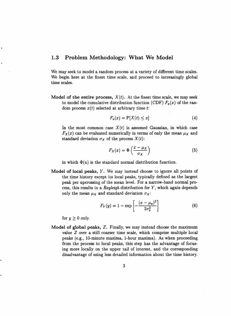
1.3 Problem Methodology: What We Model

We may seek to model a random process at a variety of different time scales. We begin here at the finest time scale, and proceed to increasingly global time scales.

Model of the entire process, X ( t ) . At the finest time scale, we may seek to model the cumulative distribution function (CDF) F,(z) of the random process z(t) selected at arbitrary time t:

Fz(z) = P[X(t) 5.1 (4)

In the most common case X ( t ) is assumed Gaussian, in which case Fx(z) can be evaluated numerically in terms of only the mean px and standard deviation ox of the process X ( t ) :

in which @(u) is the standard normal distribution function.

Model of local peaks, Y . We may instead choose to ignore all points of the time history except its local peaks, typically defined as the largest peak per upcrossing of the mean level. For a narrow-band normal process, this results in a Raylezgh distribution for Y , which again depends only the mean px and standard deviation gx:

for y 2 0 only.

Model of global peaks, 2. Finally, we may instead choose the maximum vdue 2 over a still coarser time scale, which comprise multiple local peaks (e.g., 10-minute maxima, l-hour maxima). As when proceeding from the process to local peaks, this step has the advantage of focus- ing more locally on the upper tail of interest, and the corresponding disadvantage of using less detailed information about the time history.

3

In general, the distribution function of 2 is commonly estimated from that of Y as follows:

Fz(z) = [FY(Z)IN (7) in which N here is the number of local peaks (Y values) within the duration over which 2 extends (again, 10 minutes, 1 hour, etc.) Eq. 7 assumes both that the number of peaks, N , is deterministic and that their levels are mutually independent. Neither assumption is strictly correct, but corrections generally become insignificant as we consider extremes in the upper tails of the response probability distribution.

In the Gaussian case, combining Eqs. 6-7 yields the result

E exp ( - N ~ - ( ~ - P X ) ' / ~ U $ ) (8) The MaxFits routine permits the user to select both which quantity is directly input-X(t), Y , or 2-and also to choose which quantity is to be probabilistically modelled: either X ( t ) , Y , or 2. As noted below, in the special case when the entire process X(t) is to be modelled, we permit only a single, "Hermite" distribution model.

The various distributions available within MaxFits are described in sub- sections that follow. Once estimated, Fy(y) or Fz(z ) can be used to estimate the distribution of X,, in Eq. 1, in a manner analogous to Eq. 7:

Fx,,, (x) = P[Xmax L x] = [FY (%)INy (9) = [Fz(x)lNZ (10)

If FY has been fit we use Eq. 9, in which Ny is the number of local peaks expected in time 2'. If FZ has instead been fit we use &. 10, in which Nz is the number of global peaks (e.g., number of 10-minute or 1-hour segments) in time 5".

The mean and standard deviation, px,,, and OX,,,,, corresponding to the distribution of X,, given above is found in MaxFits by numerical integration, using Gaussian quadrature procedures.

4

1.4 Uncertainty Estimates through Bootstrapping

Finally, bootstrapping methods (e.g., Efron and Tibshirani, 1993) are used here to estimate the statistical uncertainty associated with any/all of our estimated statistics of Xmm. The method is conceptually straightforward, generating multiple “equally likely” data sets by simulating, with replacement, from the original data set. Thus some of the data values will be repeated multiple times, while others will be omitted, in any single bootstrap sample (which is of the same size as the original data set). The same estimation procedure performed for the original data set is repeated for each of the bootstrapped samples, and the net statistics on the results are collected and reported.

The bootstrap method is “non-parametric” by definition, in that it operates with no additional information beside the actual data values. Alterna- tive approaches might fit a parametric model, either statistical or physical, to generate additional “equally likely” samples from which to infer sampling variability levels. Such approaches may confer advantages in some cases but are generally problem-specific; the bootstrap method is adopted here primar- ily due to its virtue of generality.

1.5 Distribution Fitting: Relation to Other Algorithms

Central to this routine is a core group of algorithms used to probabilistically model various aspects of the dynamic process of interest noted above: the process X , its local peaks Y , or its global peaks 2. The set of distribution types available are, with the sole exception of the 4moment Hermite model, the same as those available in the routine FITS, as documented most recently in RMS Report 38 (Manuel et al, 1999). Again apart from the Hermite case, this distribution set was chosen to provide relatively robust fits, preserving two or at most three moments.

In this sense, both FITS and MaxFits are intended to complement the previously distributed routine, FITTING, documented in RMS Report 14 (Win-

5

terstein et al, 1994). The FITTING routine implements relatively complex, four-moment distribution models, whose parameters are fit with numerical optimization routines. While these four-moment fits can be quite useful and faithful to the observed data, their complexity can make them difficult to automate within standard fitting algorithms, and repeated application over sets of bootstrapped samples. As noted above, however, we do include the 4moment Hermite distribution as implemented in FITTING, in view of its growing use in a variety of applications.

To focus on upper tails of interest, the user can also supply an arbitrary lower-bound threshold, xlw, above which a shifted version of a positive random variable model-exponential, Weibull, or quadratic Weibull-is fit. (In estimating statistics of the maximum response, the program automatically adjusts for the decreasing rate of response events as the threshold qaW is raised.)

6

1.6 Available Distribution Types

Specific distributions currently included in MaxFits to estimate F,(x) include the following, as catalogued by the distribution index IDIST:

IDIST=l:

IDIST=2:

IDIST=3:

IDIST=4:

IDIST=5:

IDIST=6:

IDIST=7:

IDIST=8:

IDIST=9:

Normal Distribution

Lognormal Distribution

Exponential Distribution

Weibull Distribution

Gumbel Distribution

Shifted Exponential Distribution

Shifted Weibull Distribution

Quadratic Weibull Distribution

Shifted Quadratic Weibull Distribution

IDIST=10: Four-Moment Hermite Distribution

IDIST=11: Hermite Distribution Model of Peaks, based on four moments Of

the underlying process

The distributions IDIST=l through 5 and 8 are all fit to statistical moments of a l l available data. The single-parameter exponential preserves only the mean m, of the data, while the normal, lognormal, Weibull, and Gumbel preserve both the mean and standard deviation uz estimated from the data. The quadratic Weibull preserves the first three moments of the data (mean, standard deviation, and skewness). The Hermite model (IDIST=10) is perhaps the most general, seeking to preserve the first four moments of the data (mean, standard deviation, skewness, and kurtosis). The Hermite model of peaks (IDIST=11) is special, in that it takes as input the first four moments

7

of the underlying random process X ( t ) , and provides a consistent distribution of the local peaks Y .

Most of the one-sided distributions above (exponential, Weibull, and quadratic Weibull) are also generalized here by shifting (IDIST=6, 7, and 9). These impose a user-defined lower threshold xl,, ignore data below xl,, and fit standard exponential/Weibull/quadratic Weibull models to x - xl, based on observed moments. These are perhaps the most relevant distributions when modelling local peaks, Y, which generally have a broadly skewed distribution away from a well-defined lower bound.

The result aims to provide the user with a suite of smooth probability models, to be fit throughout the body of the available data. It does not directly address various special topics of data fitting; e.g., selective tail fitting, fitting bimodal models to hybrid data, etc. Some of these issues can be addressed, in a limited way, through the use here of the shifted models (IDIST=6, 7, and 9). In this way the user can focus the distribution modelling resources on the extreme response levels of interest.

More specific tail-fitting procedures have not been given here, because optimal use of these may be rather problem-specific. In the same vein our extrema1 models are limited here to so-called “Type I” behavior, leading to (shifted) exponential distributions of peaks over a given threshold and to Gumbel distributions of annual maxima. Type I1 and I11 distributions are ill-suited to our moment fits, due to potential moment divergence (Type 11) or to the difficulty in predicting truncated distributions (Type 111) from moment information.

1.7 Limitations

An important limitation arises when the user seeks to model the entire process X ( t ) , as opposed to directly modelling its local peaks, Y, or its global peaks, 2. (As discussed in section 4.1, this choice is made by choosing the input parameter DATASWITCH=l.) In this case, MaxFits requires a model of local peaks, Y , whose distribution is consistent with moment statistics of

8

the random process X@). The only such distribution available in MaxFi t s for this purpose is IDIST=11; i.e., a model of local peaks consistent with a four-moment cubic ( “Hermite”) transformation of a Gaussian process. As a result, if the user selects DATASWITCH=l, the routine automatically forces the distribution choice IDIST=11.

Also, in this case when the user models the entire process X ( t ) , we do not permit the bootstrapping option, as this would distort the time-scale of variation of X ( t ) if its values were merely sampled with replacement over the time-axis.

Finally, NMAX, the maximum number of data, has been set to 45000. This has been set in a PARAMETER statement in the main driver program to MaxFits . This is a rather arbitrarily selected limit, and can be reset by the user without fundamental consequence.

9

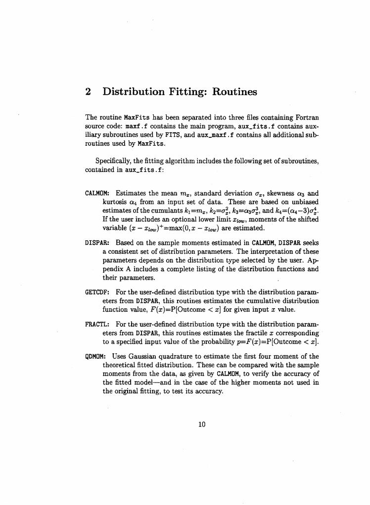
2 Distribution Fitting: Routines

The routine MaxFits has been separated into three files containing Fortran source code: maxf . f contains the main program, aux-f its. f contains am- iliary subroutines .used by FITS, and aux-maxf . f contains all additional subroutines used by MaxFits.

Specifically, the fitting algorithm includes the following set of subroutines, contained in aux-f its. f :

CALMOM Estimates the mean m,, standard deviation a,, skewness a3 and kurtosis a4 from an input set of data. These are based on unbiased estimates of the cumulants kl=mz, k2=ai, k3=a34, and k4=(a4-3)ai. If the user includes an optional lower limit $lour, moments of the shifted variable (z - zlm)+=max(O, z - %lour) are estimated.

DISPAR: Based on the sample moments estimated in CALMOM, DISPAR seeks a consistent set of distribution parameters. The interpretation of these parameters depends on the distribution type selected by the user. A p pendix A includes a complete listing of the distribution functions and their parameters.

GETCDF: For the user-defined distribution type with the distribution parameters from DISPAR, this routines estimates the cumulative distribution function value, F(z)=P[Outcome < z] for given input z value.

FRACTL: For the user-defined distribution type with the distribution parameters from DISPAR, this routines estimates the fractile z corresponding to a specified input value of the probability p=F(z)=P[Outcome < x].

QDMOM: Uses Gaussian quadrature to estimate the first four moment of the theoretical fitted distribution. These can be compared with the sample moments from the data, as given by CALMOM, to verify the accuracy of the fitted model-and in the case of the higher moments not used in the original fitting, to test its accuracy.

10

The routines GETCDF and FRACTL, which supply general distribution functions and their inverses, may also be useful in other stand-alone applications; e.g., to create a distribution library for standard FORM/SORM or simulation analyses (Madsen et al, 1986), or for use with new Inverse FORM algorithms (Ude and Winterstein, 1996).

The additional subroutines contained in aux-maxf . f are as follows:

DATAPREP: Prepares the data for the analysis. The user specifies whether the input data represent the entire process X ( t ) , the local peaks Y, or the global peaks 2. DATAPREP selects, from the input information, the appropriate data values to be retained for purposes of probabilistic modelling/fitting.

DISTINT: Finds the mean and standard deviation, px,,, and OX,,,, of the maximum value X,, by numerical integration, using Gaussian quadrature methods.

RESAMP: Generates a new, “equally likely” dataset of the same size from the original data by sampling with replacement. This is used to produce bootstrap estimates of the standard deviation of our estimates.

CALCES: Handles administrative work involved with bootstrapping, such as keeping track of running sums, etc.

11

3 Estimating Extreme Loads on Wind Tur- bines

This chapter considers how the foregoing probability models can be applied to estimate extreme bending loads on wind turbines. The database we use contains multiple 10-minute simulations of Gaussian wind fields, and corresponding in- and out-of-plane bending moment loads on a specific horizontal axis wind turbine (the Aerodynamics Experiment Phase I11 turbine; see Madsen et al, 1999 and its associated references). The turbine has a rotor diameter of 10m and a nominal rotor speed of 1.2 Hz. It is a three-bladed turbine with a hub height of 17m.

A total of 100 10-minute simulations have been performed for various choices of the mean wind speed v. These use a general-purpose, commercially available structural analysis code (ADAMS), linked with special-purpose routines to estimate aerodynamic effects (Hansen, 1996). We focus here on three cases:

1. V=14m/s, typical of nominal or “rated” wind conditions;

2. V=20m/s, the maximum or “cut-out” wind speed at which the turbine operates; and

3. V=45m/s, an extreme wind speed (e.g., 50-year level) during which the turbine is parked.

The last case is somewhat analogous to extreme winds on buildings and other stationary structures, and we may expect similar statistical behavior in this wind turbine analysis. The lower-speed cases, however, correspond to operating conditions, in which the turbine blades rotationally sample the stationary wind field. Also notable here are the systematic effects of gravity on in-plane bending: a strong sinusoidal trend is induced at the turbine operating speed. We investigate here whether various probabilistic response models can remain accurate in the face of these special features that wind turbines exhibit.

12

In particular, we study here the behavior of two different types of probabilistic models: (1) Hemite models, which seek to statistically characterize the entire random process history by a limited set of its moments; and (2) quadratic Weibull models, which seek to statistically characterize only the process peaks over a specified threshold (in this case, through corresponding moments of these peak values). Recall that the MaxFits routine implements both types of models.

3.1 Numerical Results 1: Sample Time Histories and Correlations

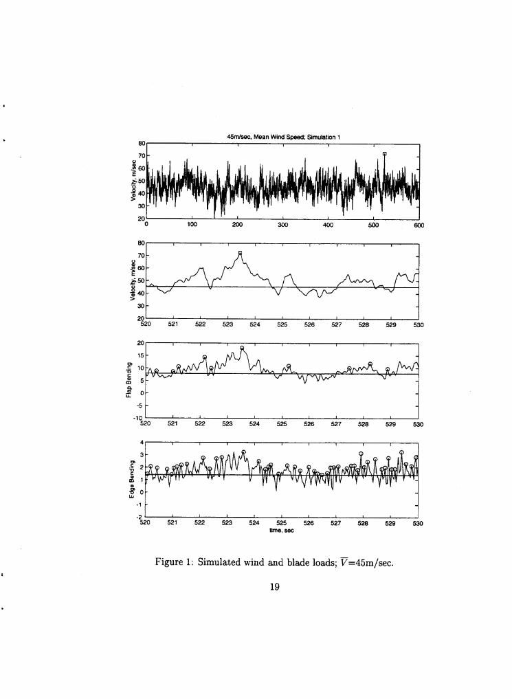
Figure 1 shows simulated wind and load time histories from one 10-minute simulation. The uppermost figure shows the entire wind input; the remaining three show enlarged, 10-second portions of the wind and load histories during which the wind input is maximized. (This maximum wind episode does not generally produce the maximum bending loads.)

To identify peaks from the response histories, we define a peak here as the largest value of the history between successive upcrossings of its mean level. Figure 1 shows the mean levels of each history by horizontal lines, and the circled response points indicate the set of peaks that are obtained. The out-of-plane (flap) bending loads are found here to roughly follow the wind speed process, although additional high-frequency content is observed. Note also that our definition of peaks (largest response per upcrossing of the mean) serves to filter out many of these high-frequency response oscillations. The edge bending loads are of less interest in this case, showing small oscillations about the mean load.

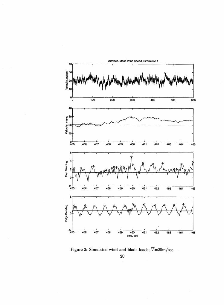
Figure 2 shows similar simulated wind and load time histories, now from a wind speed V=20m/s during which the turbine is operating. Now the effect of gravity is clearly seen in the edge bending history, which shows a strong sinusoidal component at the operating speed of roughly 1.2 Hz. The flap bending history also shows systematic variations at this frequency, although it is combined with significantly larger high-frequency content here

13

than in the edgewise case. Again, our peak identification method removes some of this high-frequency effect. Note in the edgewise case, however, that a somewhat anomalous effect can arise. While only one “large amplitude” peak is usually found per blade revolution, other “secondary”, near-zero peaks are sometimes also identified. This arises from the high-frequency small- amplitude oscillations shown by the edgewise loads about their mean level. The resulting distribution of all peaks is found in such cases to be bimodal; i.e., to possess a probability distribution model with several distinct regions of relatively high probability (“modes”). Because our models are unimodal- i.e., designed to be fit to the single most important probability “mode”-we shall find it useful in these edgewise cases to pass a higher threshold (above the mean) to exclude these secondary peaks. We shall return to this issue in the next section.

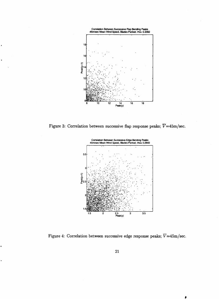
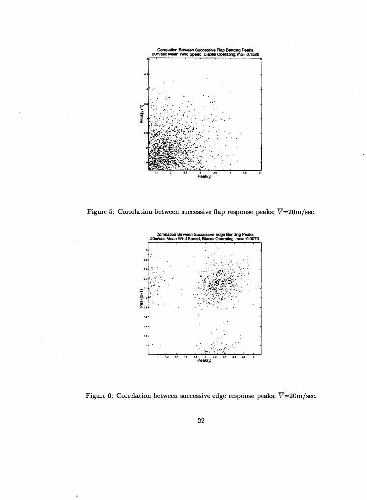
Finally, recall that to estimate the distribution of the largest peak, it is common to assume that successive peaks are mutually independent. This is the assumption inherent in our current implementation of MaxFits (see, for example, Eq. 7). To test this assumption, Figures 3 through 6 show scatter- plots of ( Y k , Y k + J , i.e., all pairs of adjacent peaks Y k and Yk+l . It is clear from the plots, and the reported correlation coefficients they contain, that the assumption of independence should not induce large modelling errors in this application. This conclusion may differ in other applications; for example, the lightly damped slow-drift response of some moored marine structures.

3.2 Numerical Results 2: Observed vs Predicted Dis- tributions of Peaks

We now test the ability of a three-moment, quadratic Weibull distribution to accurately model the simulated response peaks across various wind conditions. For illustration purposes, we again show results for the first (of the 100) 10-minute simulations. (A sample input and output file, described in the next chapter, illustrates the use of MaxFits to derive some of the results shown here.)

14

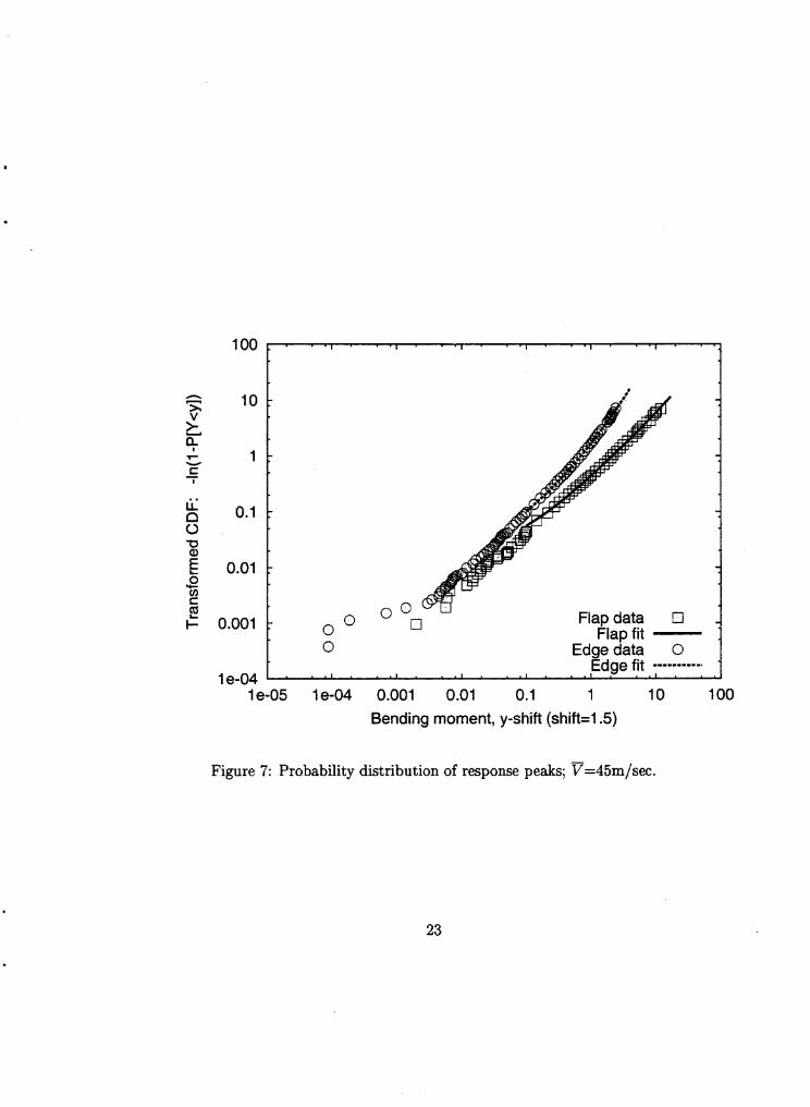
We again consider first the parked turbine (V=45m/s), whose statistical behavior may be expected to be most well-behaved. Figure 7 shows the cumulative probability distribution function Fy(y)=P[Y 5 y] of all peaks, as estimated directly from the data. Specifically, for both flap and edge cases, the peaks yi are first ordered so that y1 5 y2 5 ... 5 yn, and associated with the cumulative probabilities pi=Fy(yi)=i/(n + 1). Results are plotted on a distorted “Weibull” scale, which plots y not versus Fy(y) but rather versus - ln[l - Fy(y)]. The results, when viewed on log-log scale, should appear as a straight line if the data follow a Weibull probability distribution model.

The data here show slightly positive curvature on this Weibull scale. This suggests the value of the quadratic Weibull model, which yields a quadrat- ically varying distribution when plotted on the Weibull scale of Figure 7. This quadratic model is shown here to accurately follow both the flap and edge load data in this case.

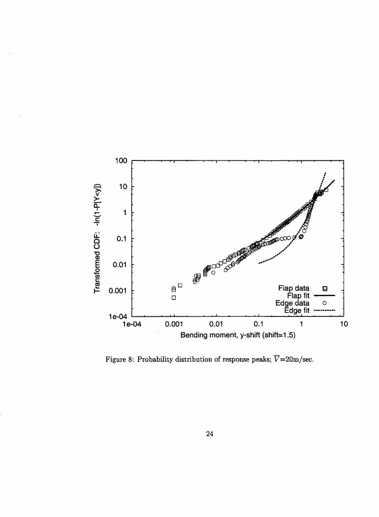
- Figure 8 shows similar Weibull scale plots of flap and edge loads in the V=20m/s case, during which the turbine is rotating. While the distribution of flap load peaks remains smooth, the distribution of edge load peaks shows a sharp change in behavior, with a “corner” located at roughly y=l. This is a consequence of the bimodal character of the edge load peaks, as discussed earlier. No smooth, single-moded distribution model can capture both the large, one-per-revolution primary peaks and the small-amplitude, secondary peaks. For both ultimate and fatigue load modelling purposes, however, these secondary peaks are of little consequence. We therefore seek to model the shifted peaks, Y - 1.5; i.e., we remove all peaks below 1.5, and report the shifted values yi=yi - 1.5 of the remaining peaks. The shifting is used to conform with quadratic Weibull models, which generally assigns probability to all outcomes y’ 2 0. Figure 9 shows the quadratic Weibull model to accurately follow the shifted edge loads, Y - 1.5. (Note that the optimal choice of shift parameter may require some trial and error; e.g., comparing goodness-of-fit measures. This is a topic of ongoing study. Note also that in using these models to predict extremes, the shift value must eventually be reinstated, to report loads in units consistent with their input values. This is done automatically in the MaxFits routine).

15

3.3 Numerical Results 3: Estimating 10-Minute Mean Maxima

Finally, we show predicted statistics of Z=max[z(t)], the maximum response over a 10-minute period. In particular, we seek here to estimate mz, the mean value of Z to be expected in an arbitrary 10-minute period. A simple, “raw” estimate of mz can be found by averaging the 100 observed maxima, Zi, from each of the 10-minute simulations:

1 100

Alternatively, we can estimate mz by fitting one of the foregoing models; e.g, a quadratic Weibull model to all response peaks (perhaps above a shifted level). Here we fit such models separately to each of the 100 simulations. Denoting pi as the estimated value of rnz from simulation i (z=l, ..., loo), we may form an analogous average of these estimates:

1 loo

One advantage of the simple, “raw” estimate z is that it is always “unbiased”; i.e., correct on average. A potential disadvantage is that because it is based on only the single observed maximum in each 10-minute history, it may show considerable variability. By instead fitting probability models to form estimates p, we hope to achieve results that (1) remain nearly unbiased and (2) show reduced scatter (specifically, standard deviation) compared with the raw estimate z. To quantify these effects we define two factors: a bias factor, defined as -

Bias (B) = = /I z (13)

and a sigma reduction factor, defined as

Sigma Reduction (SR) = 9 (14)

We hope to achieve bias factors of nearly unity, and sigma reductions f a r less than unity.

02

16

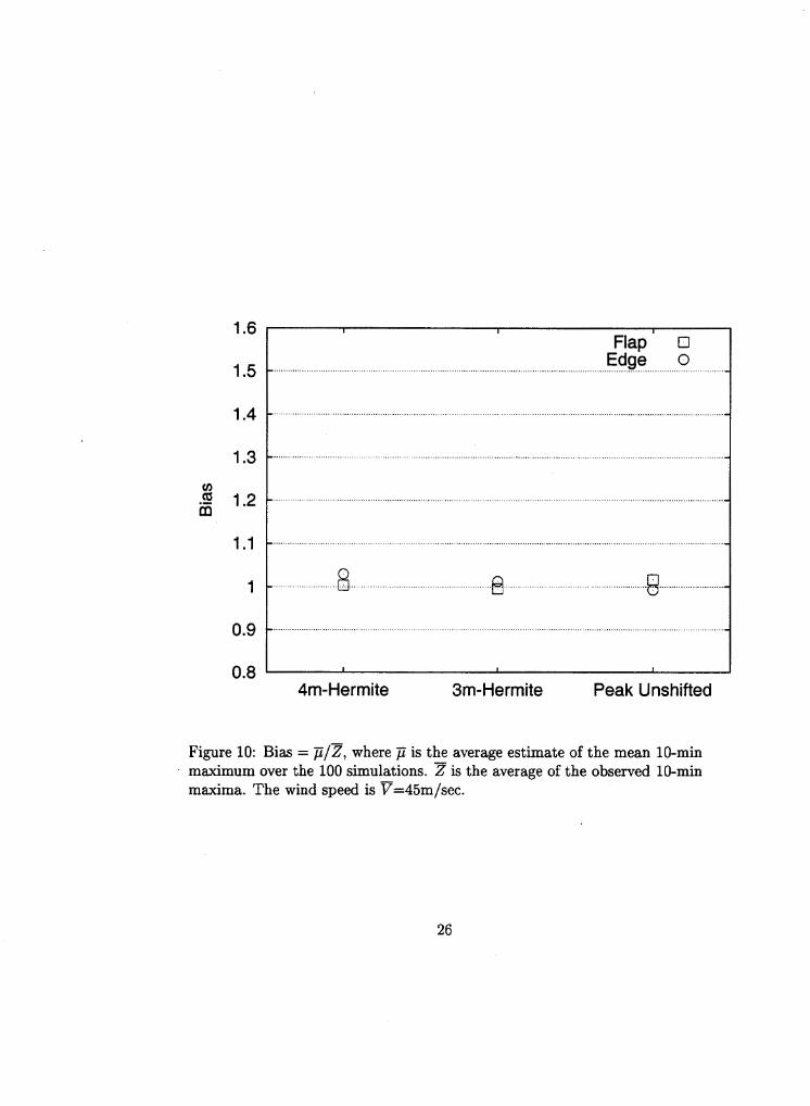
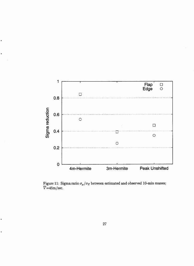
Figures 10 and 11 show bias and SR factors, respectively, for the parked turbine (v=45m/s). Three probability models are fit: a 3-moment quadratic Weibull model ( “Peak Unshifted”), and both 3- and 4-moment Hermite models of the complete random response process ~ ( t ) . (The four moment model has become the option of choice for general use. The three-moment sim- plification has been used in some mildly nonlinear wave applications, and has been recently been derived independently for wind turbine applications (Madsen et al, 1999)). Note that all models yield roughly unbiased results (B near 1.0). The 3-moment models generally achieve a sigma reduction of 0.5 or less. As might be expected, inclusion of the 4th moment, with its attendant uncertainty, leads to higher values of afi and hence SR.

Figures 12-15 show analogous bias and SR factors for the operating wind speed conditions, v=20m/s and 14m/s. Here the random process (Hermite) models, which are intended to model rather general stochastic behavior, fail to accurately capture the rotating nature of the blade response. Biases of about 10% are found from conventional (4moment) Hermite models, with considerably larger biases produced by the simpler 3-moment Hermite models.

In contrast, the quadratic Weibull (“Peak”) models remain essentially unbiased in all cases. For cases of edge loads, models have been fit both to the original data yi (“Unshifted”) and the shifted data yi - 1.5 (“Shifted”). For this particular choice of duration (T=lO-minute maxima), even the unshifted models appear reasonably accurate. Over longer durations, however, estimates become increasingly tail-sensitive, and the use of the shift has been found more beneficial in avoiding bias. Note, also, that as in the parked case, sigma reductions for these peak models all remain at roughly 0.5 or less. Nu- merical data is presented in Table l .

3.4 Summary

This chapter has demonstrated the use of both random process and random peak models to estimate extreme wind turbine loads. In particular, it has applied 3-moment random peak models (quadratic Weibull), and 3- and 4

17

moment random process models (Hermite). Both the quadratic Weibull and (4-moment) Hermite models are available within MaxFits. A sample input and output file, described in the next chapter, illustrates how the routine can be used to derive some of the results shown here.

For a parked wind turbine experiencing 50-year winds, all models have been shown to be nearly unbiased (Figure 10) and to achieve a significant reduction in our uncertainty (Figure 11) in estimating m ~ , the mean 10-minute maximum. For rotating blades during operation (at lower wind speeds), the random process models can show notable bias: roughly 10% for the 4-moment models, and appreciably more if only 3 moments are used (Figures 12-15). In contrast, the random peak models remain consistently accurate, and consistently beneficial (i.e., in reducing uncertainty) in all cases. This suggests that by modelling not the entire time history but rather its set of peaks, enough information about the rotating nature of the load process is retained to permit accurate estimates of extreme behavior.

18

a

80

7n P

45m/sec. Mean Wind Speed; Simulation 1 I I I I

30 t -I 20 I I L 520 521 522 523 524 525 526 527 528 529 530

20

15

g 10

d 5

m

c

i! -10 -:i 520 521 522 523 524 525 526 527 528 529 530

-2 t 1 1 520 521 522 523 524 525 526 527 528 529 530

time, sec

Figure 1: Simulated wind and blade loads; V=45m/sec.

19

44 20m/sec, Mean Wind Speed; Simulation 1

0' I I I 0 100 200 300 400 500 600

0' I I 1 I 1 I I I I

455 456 457 458 459 460 461 462 463 464 465

p P 4

$ 2 n ii

0

8 I 455 456 457 458 459 460 461 462 463 464 465

Figure 2: Simulated wind and blade loads; V=20m/sec. 20

a

45mlsec Mean Wind Speed, Blades Parked; mo= 0.2092 Correlation Between Successive Flap Bending Peaks

Figure 3: Correlation between successive flap response peaks; v=45m/sec.

45Wsec Mean Wtnd Speed. Blades Parked; moS 0.2843 Correlation Between Successive Edge Bending Peaks

. '.

.. . . . . . . . . . . . . . . .

. . . . . . .. ,. . . . .

. . .

1.5 2 2.5 3 3.5

Figure 4: Correlation between successive edge response peaks; v=45m/sec.

21

2om/sec Mean Whd S p e e d , Bhdes Operating; rho= 0.1526 Comlatkm Between Successive Flap Bending Peaks

4 5

... . . . . . '. .".

Figure 5: Correlation between successive flap response peaks; v=20m/sec.

2Wsec Mean Wind Speed. Blades Operating: mo= -0.0070 Correlation Between Successive Edge Bending Peaks

i " " " . " ' " ~

.. . . . .

Figure 6: Correlation between successive edge response peaks; v=20m/sec.

22

10

1

0.1

0.01

0.001

1 e-04 le-05 le-04 0.001 0.01 0.1 1 10 100

Bending moment, y-shift (shift=l.5)

Figure 7: Probability distribution of response peaks; v=45m/sec.

23

n

>r V - Y - t I

li: n 0

I

10 7 -

1 : -

0.1 : -

0.01 7

@ -

0.001 : B o Flap data 0 Flap fit -

Edge data 0 Edge fit ---------. .

1 e-04 I . I . I . I .

1 e-04 0.001 0.01 0.1 1 10 Bending moment, y-shift (shift=l.5)

Figure 8: Probability distribution of response peaks; V=20m/sec.

24

.

100

10

1

0.1

0.01 0

0 Data o

0.001 Fit ll..lll-l.

I . I . I . I .

1 e-04 0.001 0.01 0.1 1 10 Bending moment, y-shift (shift=l.5)

Figure 9: Probability distribution of shzfted response peaks above 1.5; \'=20m/sec. -

25

1.5

1.4

1.3

1.2

1.1

1

0.9

1.6 I 1 1

Flap 0 Edge 0 , -............. .... . ....... .-... ............ ..... ....... - ....... .................. ........ ........ ..... ............................................................................

0.8 I I 1 I -

4m-Hermite 3m-Hermite Peak Unshifted

Figure 10: Bias = p/z, where jZ is the average estimate of the mean 10-min maximum over the 100 simulations. z is the average of the observed 10-min maxima. The wind speed is V=45m/sec.

26

1

0.8

0.6

0.4

0.2

0

0

Flap 0 Edge 0

0 0

U 0

0

I 1 1

4m-Hermite 3m-Hermite Peak Unshifted

Figure 11: Sigma ratio aJaz between estimated and observed 10-min maxes; V=45m/sec. -

27

1.6

1.5

.4

.3

.2

.1

1

0.9

0.8

I I i i

Flap 0 Edge 0 ._ ........ ........ . .......................... ,., ........ ..... ...... .. __.__.......... ........ ................................................. . ................. ....

0' ........ , .. . .. .., . .... ,. .... .. . .. . .. ..... ... .. ......,. .. ..... ........ ........... ..... ........ ......... ........... -.

0 .. . . ..__ .. .... ... .... . .. . .. .. . . .. .. . .. ... . . ..... ..... . . ...., D... .. .,. _. ...._... ... ..... ...... .o .. .............

'U

I I 1 1

4m-Hermite 3m-Hermite Peak Unshifted Peak Shifted

Figure 12: Bias = p/Z, where p is the average estimate of the mean 10-min maximum over the 100 simulations. z is the average of the observed 10-min maxima. The wind speed is V=20m/sec.

28

1

0.8

0.6

0.4

0.2

0

I 1 1 1

Flap 0 Edge 0

0

0

0 v

0 0

0


Figure 13: Sigma ratio aJaz between estimated and observed 10-min maxes; V=20m/sec. -

29

1.6

1.5

1.4

1.3

1.2

1.1

1

0.9

0.8

I

. . . . . . . . . . . . . . . . . . . . . . . . . . . .

I

0

i

Flap 0 Edge 0

.. ..... .. . .... ... ... . .. ..._.. . . ... . .. .. .. .. .. ... . ..... ... . ......... .o .... ...... ....... ................... 0 ................. 0

....

I I 1 1


Figure 14: Bias = p/z, where p is the average estimate of the mean 10-min maximum over the 100 simulations. 7 is the average of the observed 10-min maxima. The wind speed is 8=14m/sec.

30

.

1 I I I I

Flap 0 Edge 0

08 _ ...............................................................................................................................

0.6

0.4

0

. . . . . . . . . . . . . . 0 ......

0 ' I I I I


Figure 15: Sigma ratio u,/uz between estimated and observed 10-min maxes; V=14m/sec. -

31

I Haw I 4rn-Hermite I 3m-Hermite I Peak Predictionl Peak Prediction] Data Shift = 1.5 Unshifted Prediction Prediction

20dsec Operating

0.088 3.289 0.052 3.392 0.017 4.388 0.015 3.008 0.164 3.326 Bending Edge

StdDev Mean StdDev Mean StdDev Mean StdDev Mean StdDev Mean

FlaD Bending I 5.0921 0.4941 5.524) 0.3271 4.5171 0.1211 5.0441 0.2411 --- I -I

14dsec Operating1 I I I I I I I I Edge Bending

__- --- 0.182 3.978 0.098 3.540 0.238 4.41 1 0.330 3.987 Bending Flap

0.073 2.878 0.060 2.876 0.011 4.244 0.010 2.783 0.112 2.884

Edge Bending 4.265 0.293 4.392 0.159

I Flap -__ --- 0.102 4.234 0.074 4.319

45dsec Parked

I Haw I 4rn-Hermite I 3m-Hermite I Peak Predictionl Peak Prediction1 Data Shift = 1.5 Unshifted Prediction Prediction

Odsec Operating Bias ISR Bias ISR Bias ISR Bias ISR Mean IStdDev Edae I BeEding

--- --- 0.487 0.991 0.245 0.887 0.660 1.085 0.494 5.092 Bending Flap

0.538- 0.989 0.318 1.020 0.103 1.319 0.092 0.904 0.164 3.326

14mlsec Operating Edge Bending

--- 0.550 0.998 0.297 0.888 0.721 1.106 0.330 3.987 Bending Flap

0.651 0.998 0.538 0.997 0.100 1.472 0.092 0.965 0.112 2.884

45dsec Parked ---

Edge Bending

--- --- 0.469 1.017 0.392 0.996 0.845 1.004 1.577 20.000 Bending Flap

--- 0.347 0.993 0.253 1.013 0.543 1.030 0.293 4.265 ---

Table 1: Numerical results, observed and estimated 10-minute extremes.

32

4 Input Format and Wind Turbine Example

We will illustrate the use of MaxFits here through a simple example, drawn from among the wind turbine simulation cases discussed previously. In particular, we consider here the flap bending response of a parked wind turbine blade. The input is discussed in the following paragraph. The output is discussed in the next section. The data set analyzed here contains ten minutes of response data for a parked wind turbine blade subjected to a simulated Gaussian wind field with 45m/s mean wind speed and 15% turbulence inten- sity (C.O.V. = .15).

The input file is stored in wind.dat. This file corresponds to the flapwise bending time series shown in Figure 1.

4.1 Runtime Input: Batch Mode

We desire the following situation:

1. Results should be written to a file named wind. out

2. Distribution results are to be written for 20 probability values ranging from 1/20 to 1-1/20.

3. The time history data is stored in the file wind. dat

4. The user desires to fit a shifted quadratic Weibull distribution ( IDIST=9) to these data. IDIST=8 should only be used if it is certain the mean of the underlying process equals 0. If this is not the case the fit should be shifted over the mean, or any other threshold if preferred.( Although it is inconvenient for the user to have to determine the mean of the process, there is no other method. The only way MaxFits $an determine the mean is if the entire process is input. In this case if the user specifies a value of 7.896 for XLOW, MaxFits will use the mean of the process as threshold.)

33

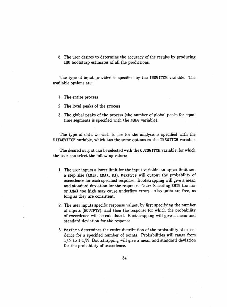
5. The user desires to determine the accuracy of the results by producing 100 bootstrap estimates of all the predictions.

The type of input provided is specified by the INSWITCH variable. The available options are:

1. The entire process

2. The local peaks of the process

3. The global peaks of the process (the number of global peaks for equal time segments is specified with the NSEG variable).

The type of data we wish to use for the analysis is specified with the DATASWITCH variable, which has the same options as the INSWITCH variable.

The desired output can be selected with the OUTSWITCH variable, for which the user can select the following values:

1. The user inputs a lower limit for the input variable, an upper limit and a step size (XMIN, XMAX, DX). MaxFits will output the probability of exceedence for each specified response. Bootstrapping will give a mean and standard deviation for the response. Note: Selecting X M I N too low or XMAX too high may cause underflow errors. Also units are free, as long as they are consistent.

2. The user inputs specific response values, by first specifying the number of inputs (NOUTPTS), and then the response for which the probability of exceedence will be calculated. Bootstrapping will give a mean and standard deviation for the response.

3. MaxFits determines the entire distribution of the probability of exceedence for a specified number of points. Probabilities will range from 1/N to 1-l/N. Bootstrapping will give a mean and standard deviation for the probability of exceedence.

34

4. The user inputs specific probability levels, by first specifying the num- bers of inputs (NOUTPTS), and then the probability of exceedence for which the associated response will be calculated. Bootstrapping will give a mean and standard deviation for the probability of exceedence.

The previous options will cause the input lines to differ, depending on the output specified on the second line of the batch file. Examples of input for all 4 possible output options are given. The batch file for the example is named wind. in, and contains the following input lines:

wind. out 1 2 3 20 10. 10. 100 wind. dat 9 7.896

: Name of output file : INSWITCH,DATASWITCH, OUTSWITCH : N, number and range of probability levels , 1/N, 1-l/N : Duration of input file and target period : Number of bootstrap samples : Name of input file : Distribution type (IDIST), see Section 1.6 for definitions : XLOW, shift only for shifted distributions

Alternatively the following batch files can be used for OUTOPT = 1,2,4 respectively:

wind. out 1 2 1 8 . 20. 1. 10. 10. 100 wind. dat 9 7.896

wind. out 1 2 2

: Name of output file : INSWITCHIDATASWITCH, OUTSWITCH : XMIN, XMAX, DX, : Duration of input file and target period : Number of bootstrap samples : Name of input file : Distribution type (IDIST), see Section 1.6 for definitions : XLOW, shift only for shifted distributions

: Name of output file : INSWITCH,DATASWITCH, OUTSWITCH

35

3

15. 20. Xnoutpts

10. 10. 100 wind. dat 9 7.896

wind. out 1 2 4 3

0.01 0.001 0.0001 Pnout , pt o

10. 10. 100 wind. dat 9 7.896

: NOUTPTS, no. of exceedence probabilities to be calculated : First fractile for which P will be calculated : Second extreme for which P will be calculated : Third extreme for which P will be calculated : Nth extreme for which MaxFits will calculated the probability

: Duration of input file and target period : Number of bootstrap samples : Name of input file : Distribution type (IDIST), see Section 1.6 for definitions : XLOW, shift only for shifted distributions

of exceedence

: Name of output file : INSWITCH,DATASWITCH, OUTSWITCH : NOUTPTS, no. of probabilities for which fractiles will be

: First probability of exceedence : Second probability of exceedence : Third probability of exceedence : Nth probability of exceedence for which MaxFits will

: Duration of input file and target period : Number of bootstrap samples : Name of input file : Distribution type (IDIST), see Section 1.6 for definitions : XLOW, shift only for shifted distributions

calculated

calculate the fractile

By typing the following command:

maxfits C wind.in

a file named wind. out will be written whose content is discussed in the next section. During the execution the user will be prompted for terminal inputs. These can simply be ignored (or directed toward the null device) in this batch mode operation.

36

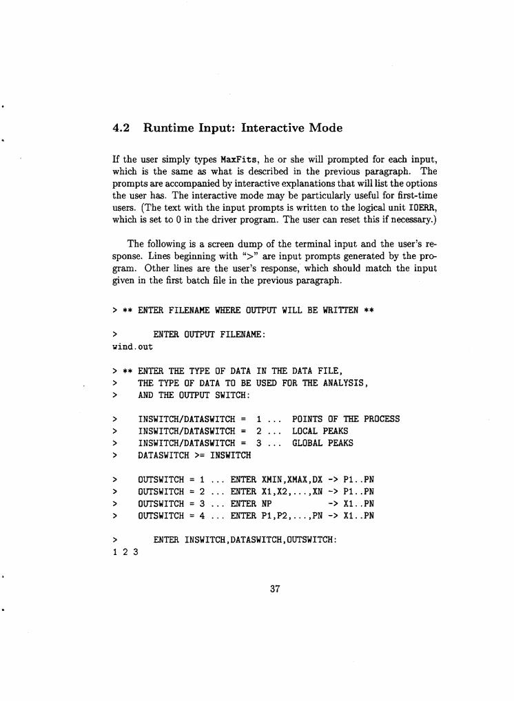
4.2 Runtime Input: Interactive Mode

If the user simply types MaxFits, he or she will prompted for each input, which is the same as what is described in the previous paragraph. The prompts are accompanied by interactive explanations that will list the options the user has. The interactive mode may be particularly useful for first-time users. (The text with the input prompts is written to the logical unit IOERR, which is set to 0 in the driver program. The user can reset this if necessary.)

The following is a screen dump of the terminal input and the user’s response. Lines beginning with “>” are input prompts generated by the program. Other lines are the user’s response, which should match the input given in the first batch file in the previous paragraph.

> ** ENTER FILENAME WHERE OUTPUT WILL BE WRI’ITEN ** > ENTER OUTPUT FILENAME: wind. out

> ** ENTER THE TYPE OF DATA IN THE DATA FILE, > THE TYPE OF DATA TO BE USED FOR THE ANALYSIS, > AND THE OUTPUT SWITCH:

> INSWITCH/DATASWITCH = 1 . . . POINTS OF THE PROCESS > INSWITCH/DATASWITCH = 2 . . . LOCAL PEAKS > INSWITCH/DATASWITCH = 3 . . . GLOBAL PEAKS > DATASWITCH >= INSWITCH

> OUTSWITCH = 1 . . . ENTER XMIN,XMAX,DX -> Pl..PN > OUTSWITCH = 2 . . . ENTER Xl,X2, . . . , XN -> Pl..PN > OUTSWITCH = 3 . . . ENTER NP -> Xi. .PN > OUTSWITCH = 4 . . . ENTER Pl,P2, . . . , PN -> Xl..PN

> ENTER INSWITCH,DATASWITCH,OUTSWITCH: 1 2 3

37

> ** ENTER NUMBER OF PROBABILITIES FOR THE DISTRIBUTION OF XMAX 20

> ** ENTER THE DURATION OF THE DATA FILE > AND THE TARGET DURATION FOR THE PREDICTION: > ASSURE TTARGET IS SUFFICIENTLY LONG > TO CONTAIN AT LEAST ONE CYCLE

> Ttot ,Ttarget : 10. 10.

> ** ENTER THE NUMBER OF BOOTSTRAP SAMPLES TO BE TAKEN: > FOR NO BOOTSTRAPPING ENTER bsN=O > bsN: 100

> ** ENTER FILENAME WHERE DATA ARE STORED,

> ENTER INPUT FILENAME: wind. dat

> ** ENTER IDIST =INDEX OF DISTRIBUTION TYPE TO BE FIT > CURRENT OPTIONS: > IDIST = 1 . . . NORMAL > IDIST = 2 . . . LOGNORMAL > IDIST = 3 . . . EXPONENTIAL > IDIST = 4 . . . WEIBULL > IDIST = 5 ... GUMBEL > IDIST = 6 . . . SHIFTED EXPONENTIAL > IDIST = 7 . . . SHIFTED WEIBUU > IDIST = 8 . . . QUADRATIC WEIBULL > IDIST = 9 . . . SHIFTED QUADRATIC WEIBULL > IDIST = 10 . . . HERMITE (PROCESS) > IDIST = 11 . . . HERMITE (PEAKS)

> ENTER IDIST:

38

> YOU HAVE SELECTED A SHIFTED DISTRIBUTION MODEL

> ** ENTER XLOW =LOWER BOUND THRESHOLD, BELOW WHICH > ALL DATA WILL BE IGNORED 9 > ENTER XLOW : 7.896

4.3 Output Format and Wind Turbine Example

Below is the output file wind. out that resulted from the manual input listed in the previous paragraph. The format is the same for all output options. Note that the output is formatted such that it can be directly plotted using gnuplot. The lines starting with # will be treated as comments by gnuplot.

The first section echoes the input, and how much data was actually used for the analysis.

The second section provides summary statistics for the data file consid- ered. These include on the first line the sample moments from the data, and on the second line the standard deviation of the bootstrap predictions.

The third section gives the moments that are implied by the fitted distribution in the same way as they are given for the original data.

The fourth section reports the distribution parameters. The standard deviation of the bootstrap predictions is given on the second the. The definition of the distribution parameters is given in Appendix A of the fits manual (Manuel et al, 1999).

The fifth section gives the mean and standard deviation of the distribution of the extreme value in the target period. The bootstrap standard deviations of these values are reported on the second line.

39

The last section reports the actual distribution of the extreme value in the target period. The first column reports the fractiles that were calculated from the specified probability levels in the input. The second column reports the bootstrap standard deviation of each predicted fractile, and indicates the accuracy of the prediction. The third column reports the probability levels that were input by the user. The fourth column reports the standard deviations of, in this case, the 100 predictions of the probability levels. As the probability levels were input here this column consists of zeros.

# # RESULTS FOR : wind. dat # TIME DURATION OF DATABASE: 10.00 # # # # # # # # # # # # # # # # # # 1)

# # # #

#

CONTAINING: 15000 POINTS OF THE PROCESS TARGET TIME DURATION: 10.00 DIST TYPE SELECTED: SHIFTED QUADRATIC W

FITTED TO: 1041 LOCAL PEAKS NO. OF BOOTSTRAP SAMPLES: 100

** N O T E : MOMENTS, DIST PARMS APPLY HERE TO X-XLOW; XLOW= 0.7896E+01

MOMENTS FROM SAMPLE DATA ( MEAN, SIGMA, SKEWNESS, KURTOSIS) data: 0.2012E+Ol 0.1806E+Ol O.l537E+Ol 0.5965E+01 s tdv: 0.5404E-01 0.6229E-01 0.1127E+00 0.6584E+00

MOMENTS FROM FITTED DIST ( MEAN, SIGMA, SKEWNESS, KURTOSIS) data: 0.2012E+01 0.1807E+Ol 0.1536E+Ol 0.6179~+01 Stdv: 0.5403E-01 0.6224E-01 0.1129E+OO 0.6058E+00

DISTRIBUTION PARAMETERS (SEE DOCUMENTATION FOR DEFINITION) data: -0.712lE-01 0.2166E+Ol O.l041E+Ol 0.8963E+00 -0.2372E-01 StdV: 0.4817E-01 0.1350E+00 0.7607E-02 0.2072E-01 0.1989E-01

40

# # # # data: # stdv: # # # X

0.1772E+02 0.1807E+02 0.1833E+02 0.1855E+02 0.1874E+02 0.1892E+02 0.1910E+02 0.1927E+02 0.1944E+02 0.1961E+02 0.1979E+02 0.1998E+02 0.2018E+02 0.2040E+02 0.2063E+02 0.2090E+02 0.2122E+02 0.2161E+02 0.2214E+02 0.2301E+02

MEAN STDV (of MAX response i n Ttarget): 19.97 1.57 0.63 0.18

As the quadratic Weibull distribution uses only three parameters, only the first three statistical moments can be reproduced by the fitted distribution. The kurtosis will differ somewhat.

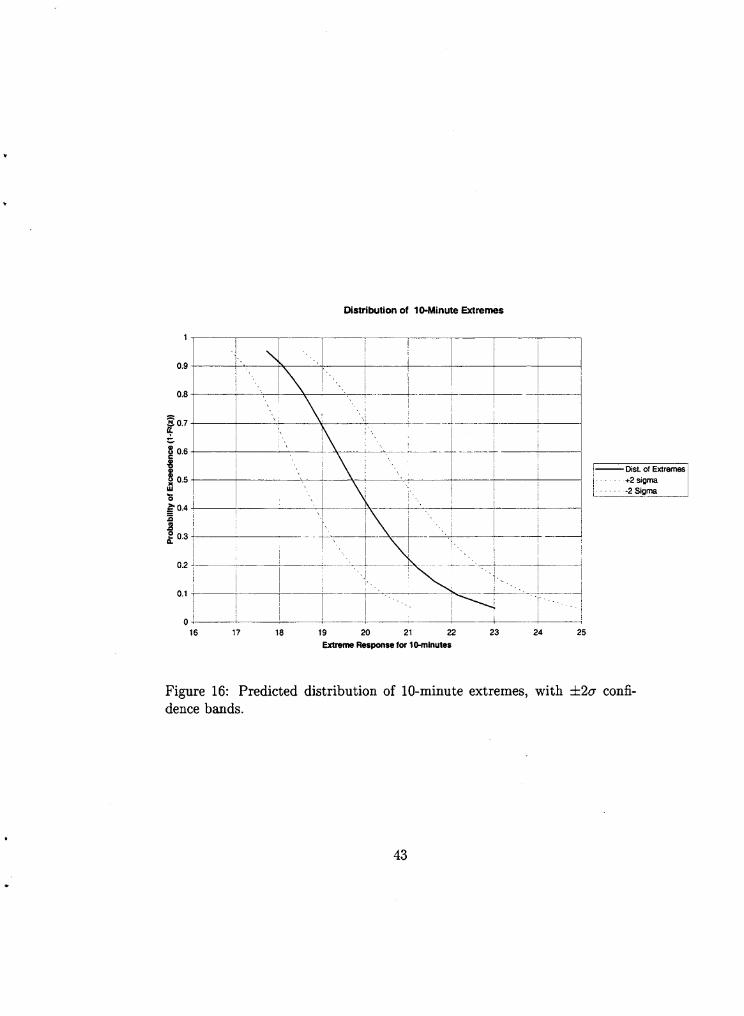
The original data, and the quadratic Weibull fit, are shown in Figure 7. Figure 16 shows the distribution of the ten-minute extreme flap bending response produced by MaxFits, and lines reflecting this value plus and minus

41

Distribution of 1Minute Extremes

16 17 10 19 20 21 22 23 24 25 Extreme Response for lO-minutes

Figure 16: Predicted distribution of 10-minute extremes, with iz2a confi- dence bands.

43

5 References Manuel, L., T. Kashef and S.R. Winterstein (1999). Moment-based probability

modelling and extreme response estimation: The FITS routine (Ver. 1.2), Rept. RMS-38, Reliability of Marine Structures Program, Dept. of Civ. & Environ. Eng., Stanford University.

De Jong, R. and S.R. Winterstein (1998). Probabilistic models of dynamic response and bootstrap-based estimates of extremes: the routine Maxfits, Rept. RMS-34, Reliability of Marine Structures Program, Dept. of Civ. & Environ. Eng., Stanford University.

Engebretsen, K. and S.R. Winterstein (1998). Probability-based design loads and responses of floating structures: extreme slow drifl motion and tether tension, Rept. RMS-30, Reliability of Marine Structures Program, Dept. of Civ. & Environ. Eng., Stanford University.

Winterstein, S.R. and K. Engebretsen (1998). Reliability-based prediction of design loads and responses for floating ocean structures. Proc., 17th Intl. Oflshore Mech. Arctic Eng. Symp., ASME, .

Efron, B. and R.J. Tibshirani (1993). An introduction to the bootstrap, C h a p man & Hall.

Manuel, L., T. Kashef and S.R. Winterstein (1999). Moment-based probability modelling and extreme response estimation: The FITS routine (Ver. 1.2), Rept. RMS-38, Reliability of Marine Structures Program, Dept. of Civ. & Environ. Eng., Stanford University.

Winterstein, S.R., C.H. Lange, and S. Kumar (1994). FITTING: A subrou- tine to fit four moment probability distributions to' data, Rept. RMS-14, Reliability of Marine Structures Program, Civil Eng. Dept., Stanford Uni- versity.

Madsen, H.O., S. Krenk, and N.C. Lind (1986). Methods of structural safety, Prentice-Hall, Inc., New Jersey.

Ude, T.C. and S.R. Winterstein (1996). IFORM: An inverse-FORM row tine to estimate response levels with specified return periods, Rept. TN-3, Reliability of Marine Structures Program, Civil Eng. Dept., Stanford Uni- versity.

Madsen, P.H., K. Pierce and M. Buhl (1999). Predicting ultimate loads for wind turbine design. Proc., 1999 ASME Wind Energy Symposium, 37th AIAA Aero. Sci. Mtg., 355-364.

Hansen, A.C. (1996). Users guide to the wind turbine dynamics computer

44

programs YawDyn and AeroDyn for ADAMS, Mech. Eng. Dept., Univ. of Utah.

Madsen, P.H., K. Pierce and M. Buhl (1999). Predicting ultimate loads for wind turbine design. Proc., 1999 ASME Wind Energy Symposium, 37th AIAA Aero. Sci. Mtg., 355-364.

Manuel, L., T. Kashef and S.R. Winterstein (1999). Moment-basedprobability modelling and extreme response estimation: The FITS routine (Ver. 1.2), Rept. RMS-38, Reliability of Marine Structures Program, Dept. of Civ. & Environ. Eng., Stanford University.

45

DISTRIBUTION

T. Almeida TPI Composites Inc. 373 Market Street Warren, RI 02885

H. Ashley Dept. of Aeronautics and

Stanford University Stanford, CA 94305

Astronautics Mechamcal Engr.

K. Bergey University of Oklahoma Aero Engineering Department Norman, OK 73069

R. Blakemore Enron Wind Corp. 13681 Chantico Road Tehachapi, CA 93561

C. P. Butterfield NREL 16 17 Cole Boulevard Golden, CO 80401

G. Bywaters Northern Power Systems Box 999 Waitsfield,VT 05673

J. Cadogan Office of Geothermal & Wind

Technology EE-12 U.S. Department of Energy 1000 Independence Avenue SW Washington, DC 20585

D. Cairns Montana State University Mechanical & Industrial Engineering Dept. 220 Roberts Hall Bozeman, MT 59717

S . Calvert Office of Geothermal & Wind

Technology EE- 12 U.S. Department of Energy 1000 Independence Avenue SW Washington, DC 20585

J. Chapman OEM Development Corp. 840 Summer St. Boston, MA 02127-1533

Kip Cheney PS Enterprises 222 N. El Segundo, #576 Palm Springs, CA 92262

C. Christensen Enron Wind Corp. 1368 1 Chantico Road Tehachapi, CA 93561

R. N. Clark USDA Agricultural Research Service P.O. Drawer 10 Bushland, TX 79012

J. Cohen Princeton Economic Research, Inc. 1700 Rockville Pike Suite 550 Rockville, MD 20852

C. Coleman Northern Power Systems Box 999 Waitsfield, VT 05673

C. A. Cornell Civil Engineering Department Stanford University Stanford, CA 94305

K. J. Deering The Wind Turbine Company 5 15 1 16th Avenue NE No. 263 Bellevue, WA 98004

A. J. Eggers, Jr. RANN, Inc. 744 San Antonio Road, Ste. 26 Palo Alto, CA 94303

D. M. Eggleston DME Engineering 1605 W. Tennessee Ave. Midland, TX 79701-6083

L. M. Fitzwater (5) Civil Engineering Department Stanford University Stanford, CA 94305

P. R. Goldman Director

* Office of Geothermal & Wind Technology

EE- 12 US. Department of Energy 1000 Independence Avenue SW Washington, DC 20585

G. Gregorek Aeronautical & Astronautical Dept. Ohio State University 2300 West Case Road Columbus, OH 43220

D. Griffin GEC 5729 Lakeview Drive NE, Ste. 100 Kirkland, WA 98033

C. Hansen Windward Engineering 466 1 Holly Lane Salt Lake City, UT 84 1 17

C. Hedley Headwaters Composites 105 E. Adam St. Three Forks, MT 59752

S. Hock Wind Energy Program NREL 16 17 Cole Boulevard Golden, CO 80401

Bill Holley 373 1 Oakbrook Pleasanton, CA 94588

K. Jackson Dynamic Design 123 C Street Davis, CA 956 16

E. Jacobsen Enron Wind 13000 Jameson Rd. Tehachapi, CA 93561

M. Kramer Foam Matrix, Inc. PO Box 6394 Malibu CA 90264

D. Malcolm GEC 5729 Lakeview Drive NE, Ste. 100 Kirkland, WA 98033

J. F. Mandell Montana State University 302 Cableigh Hall Bozeman, MT 597 17

T. McCoy GEC 5729 Lakeview Drive NE, Ste. 100 Kirkland, WA 98033

L. McKittrick ‘Montana State University Mechanical & Industrial Engineering Dept. 220 Roberts Hall Bozeman, MT 5971 7

P. Migliore NREL 161 7 Cole Boulevard Golden, CO 80401

W. Musial NREL 16 17 Cole Boulevard Golden, CO 80401

NWTC Library (5) NREL 1617 Cole Boulevard Golden, CO 80401

B. Neal USDA Agricultural Research Service P.O. Drawer 10 Bushland, TX 790 12

V. Nelson Department of Physics West Texas State University P.O. Box 248 Canyon, TX 790 16

J. W. Oler Mechanical Engineering Dept. Texas Tech University P.O. Box 4289 Lubbock, TX 79409

T. Olsen Tim Olsen Consulting 1428 S . Humboldt St. Denver, CO 80210

J. Richmond MDEC 3368 Mountain Trail Ave. Newbury Park, CA 91320

Michael Robinson NREL 1 6 17 Cole Boulevard Golden, CO 80401

D. Sanchez U.S. Dept. of Energy Albuquerque Operations Office P.O. Box 5400 Albuquerque, NM 87185

L. Schienbein CWT Technologies, Inc. 4006 S. Morain Loop Kennewick, WA 99337

R. Sherwin Atlantic Orient PO Box 1097 Norwich, VT 05055

Brian Smith NREL 16 17 Cole Boulevard Golden, CO 80401

K. Starcher AEI West Texas State University P.O. Box 248 Canyon, TX 79016

F. S. Stoddard 79 S . Pleasant St. #2A Amherst, MA 0 1002

A. Swift University of Texas at El Paso 320 Kent Ave. El Paso, TX 79922

R. W. Thresher NREL 16 17 Cole Boulevard Golden, CO 80401

S . Tsai Stanford University Aeronautics & Astronautics Durand Bldg. Room 38 1 Stanford, CA 94305-4035

W. A. Vachon W. A. Vachon 8~ Associates P.O. Box 149 Manchester, MA 01944

C. P. van Dam Dept. of Mech. and Aero. Eng. Univ. of California, Davis One Shields Avenue Davis, CA 95616-5294

B. Vick USDA, Agricultural Research Service P.O. Drawer 10 Bushland, TX 79012

R. E. Wilson Mechanical Engineering Dept. Oregon State University Corvallis, OR 9733 1

S . R. Winterstein (5) Civil Engineering Department Stanford University Stanford, CA 94305

M. Zuteck MDZ Consulting 931 Grove Street Kemah, TX 77565

M.S. 0557 M.S. 0557 M.S. 0708 M.S. 0708 M.S. 0708 M.S. 0708 M.S. 0708 M.S. 0708 M.S. 0708 M.S. 0708 M.S. 0708 M.S. 0708 M S . 0708 M.S. 0708 M.S. 0847 M.S. 0847 M.S. 1490 M.S. 0958 M.S. 0612

M.S. 0899 M S . 9018

T. J. Baca, 9125 T. G. Came, 9124 H. M. Dodd, 6214 (25) T. D. Ashwill, 6214 D. E. Berg, 6214 R. R. Hill, 6214 P. L. Jones 6214 D. L. Laird, 6214 D. W. Lobitz, 6214 J. Ortiz, 6214 M. A. Rumsey, 6214 H. J. Sutherland, 6214 P. S. Veers, 6214 J. Zayas, 6214 K. E. Metzinger, 9126 D. R. Martinez, 1902 A. M. Lucero, 12660 M. Donnelly, 1472 Review & Approval Desk, 9612 For DOE/OSTI Technical Library, 9616 (2) Central Technical Files, 8945-1

estimation of extremes from limited time histories: the .../67531/metadc723878/m2/1/high... ·...

Documents