estimation of dynamic discrete choice models by maximum
TRANSCRIPT

DI
SC
US
SI
ON
P
AP
ER
S
ER
IE
S
Forschungsinstitut zur Zukunft der ArbeitInstitute for the Study of Labor
Estimation of Dynamic Discrete Choice Models by Maximum Likelihood and the Simulated Method of Moments
IZA DP No. 8548
October 2014
Philipp EisenhauerJames J. HeckmanStefano Mosso

Estimation of Dynamic Discrete Choice Models by Maximum Likelihood and the
Simulated Method of Moments
Philipp Eisenhauer University of Chicago
James J. Heckman University of Chicago, CEHD,
American Bar Foundation and IZA
Stefano Mosso University of Chicago
Discussion Paper No. 8548 October 2014
IZA
P.O. Box 7240 53072 Bonn
Germany
Phone: +49-228-3894-0 Fax: +49-228-3894-180
E-mail: [email protected]
Any opinions expressed here are those of the author(s) and not those of IZA. Research published in this series may include views on policy, but the institute itself takes no institutional policy positions. The IZA research network is committed to the IZA Guiding Principles of Research Integrity. The Institute for the Study of Labor (IZA) in Bonn is a local and virtual international research center and a place of communication between science, politics and business. IZA is an independent nonprofit organization supported by Deutsche Post Foundation. The center is associated with the University of Bonn and offers a stimulating research environment through its international network, workshops and conferences, data service, project support, research visits and doctoral program. IZA engages in (i) original and internationally competitive research in all fields of labor economics, (ii) development of policy concepts, and (iii) dissemination of research results and concepts to the interested public. IZA Discussion Papers often represent preliminary work and are circulated to encourage discussion. Citation of such a paper should account for its provisional character. A revised version may be available directly from the author.

IZA Discussion Paper No. 8548 October 2014
ABSTRACT
Estimation of Dynamic Discrete Choice Models by Maximum Likelihood and the Simulated Method of Moments*
We compare the performance of maximum likelihood (ML) and simulated method of moments (SMM) estimation for dynamic discrete choice models. We construct and estimate a simplified dynamic structural model of education that captures some basic features of educational choices in the United States in the 1980s and early 1990s. We use estimates from our model to simulate a synthetic dataset and assess the ability of ML and SMM to recover the model parameters on this sample. We investigate the performance of alternative tuning parameters for SMM. JEL Classification: C13, C15, C35, I21 Keywords: returns to education, dynamic discrete choice, simulation-based estimation Corresponding author: Philipp Eisenhauer Department of Economics The University of Chicago 1126 East 59th Street Chicago, IL 60637 USA E-mail: [email protected]
* We thank George Yates for numerous valuable comments, for excellent computational assistance in developing the maximum likelihood estimator used in this paper, and for assisting in the study of accuracy bounds for the computational algorithm. We thank Edward Sung and Jake Torcasso for their outstanding research assistance. We have benefited greatly from comments received from Chris Flinn, Kenneth Judd, Michael Keane, Bernard Salanié, Petra Todd, and Stefan Wild. We thank the editor and anonymous referees for their valuable comments. This research was supported in part by the American Bar Foundation, the Pritzker Children’s Initiative, the Buffett Early Childhood Fund, NICHD 5R37HD065072, 5R01HD054702, the Human Capital and Economic Opportunity Global Working Group - an initiative of the Becker Friedman Institute for Research in Economics - funded by the Institute for New Economic Thinking (INET), and an anonymous funder. Philipp Eisenhauer thanks Prof. Wolfgang Franz and the Centre for European Economic Research (ZEW Mannheim) for their support. The views expressed in this paper are those of the authors and not necessarily those of the funders or commentators mentioned here. The website for this paper is https://heckman.uchicago.edu/ MLvsSMM.

Estimation of Dynamic Models 2
1 Introduction
Economic science uses economic theory to guide the interpretation of economic data and to shape
policy. Kenneth Wolpin is a model economic scientist who integrates theory and data in a rigorous
fashion. He summarizes his philosophy toward empirical research in Wolpin (2013). He is a ma-
jor contributor to structural econometrics with particular emphasis on the study of dynamic discrete
choice models. His contributions are both methodological and empirical. His methodological re-
search focuses on promoting methods to increase the reliability of algorithms for structural estimation
(Eckstein and Wolpin, 1989; Keane et al., 2011) and developing techniques to simplify their empirical
implementation. His research on interpolation methods to solve dynamic discrete choice models with
a large state space (Keane and Wolpin, 1994) is a prominent example. In his empirical contributions,
he extensively applies theory-motivated methods to investigate many important issues such as edu-
cational attainment (Eckstein and Wolpin, 1999; Keane and Wolpin, 1997), the role of credit constraints
in educational attainment (Keane and Wolpin, 2001), and labor market dynamics (Lee and Wolpin,
2006, 2010).
This paper contributes to the literature on estimating dynamic discrete choice models. It investi-
gates the empirical performance of widely used versions of simulated method of moments (SMM),
a computationally tractable method for estimating complex structural models. SMM estimates pa-
rameters by fitting a vector of empirical moments to their theoretical counterparts simulated from a
structural model (McFadden, 1989). We compare its performance against standard maximum likeli-
hood (ML) estimation.1
1Alternative estimation methods have been proposed to overcome the rigidities and complexities
of ML estimation. Most require the analyst to characterize the likelihood function but simplify its
computation. One of the most popular methods, simulated ML (SML), substitutes the exact likelihood
function with a simulated one. An example is the Hajivassiliou-Geweke-Keane (HGK-SML) estimator
(Geweke, 1989; Hajivassiliou and McFadden, 1998; Keane, 1994) used for multinomial probit estima-
tion. Approximations of the dynamic programming problem have often been combined with SML in
models with a large state space (Keane and Wolpin, 1994). Another popular method is the conditional

Estimation of Dynamic Models 3
We estimate a deliberately simplified dynamic discrete choice model of schooling based on a sample
of white males from the National Longitudinal Survey of Youth (1979) using ML. Our model is more
restrictive compared to standard dynamic discrete choice models (Keane and Wolpin, 1997, 2001) with
respect to the number of choices and the timing of decisions and outcomes. We restrict agents to binary
choices and our model is based on educational states. This allows us to evaluate the likelihood ana-
lytically, without the need for any simulation or interpolation (Keane, 1994), which provides a clean
comparison of ML against simulation-based estimation methods such as SMM. Using the estimates of
model parameters, we simulate a synthetic dataset. In a series of Monte Carlo studies we compare es-
timates based on our precisely calculated ML with those from widely used, computationally tractable
versions of SMM. Because our synthetic sample is derived from real data, our analysis provides useful
lessons on the performance of SMM for the estimation of structural models.2
SMM has been used to estimate models of job search (Flinn and Mabli, 2008), educational and oc-
cupational choices (Adda et al., 2013, 2011), household choices (Flinn and Del Boca, 2012), stochastic
volatility models (Andersen et al., 2002; Raknerud and Skare, 2012), and dynamic stochastic general
equilibrium models (Ruge-Murcia, 2012). SMM can be used for any model, however complex or dif-
ficult to compute the likelihood, as long as it is possible to simulate it. Under conditions presented
in the literature, the SMM estimator is consistent and asymptotically normal (Gouriéroux and Mon-
fort, 1997). If the score vector for SMM happens to be correctly specified, then SMM is asymptotically
efficient (Gallant and Tauchen, 1996; Gouriéroux et al., 1993).3
choice probabilities (CCP) algorithm first proposed by Hotz and Miller (1993) and recently extended
to allow for unobserved heterogeneity (Arcidiacono and Miller, 2011). Using CCP, a consistent esti-
mator of the model parameters can be derived without the need of the full solution of the dynamic
programming problem. The CCP method, however, restricts the flexibility of the estimable models by
imposing assumptions which limit the dependence among successive choices. SMM is a more general
alternative to ML estimation.2As in Skrainka (2011), we use simulation experiments in realistic settings to investigate the finite
sample behavior of widely-used estimators.3See Nickl and Pötscher (2010) and Gach and Pötscher (2011) for recent additional results.

Estimation of Dynamic Models 4
Implementing any estimation strategy requires numerous choices. In the case of SMM, users have
discretion in selecting: (1) the moments used in estimation, (2) the number of replications used to
compute the simulated moments, (3) the moment weighting matrix, and (4) the algorithm used for
optimization. It is unclear how such choices affect the performance of the SMM estimator and how
they depend on the structure of the model estimated. We propose diagnostic tools to test their validity.
We suggest a Monte Carlo procedure that allows SMM users to gain confidence for their particular
implementation of the algorithm. We present a new optimization algorithm for solving derivative-
free nonlinear least-squares problems that is well-suited for conventional SMM implementations. A
benchmarking exercise demonstrates significant speed improvements compared to the algorithms
commonly used in the literature. Combining state of the art optimization methods with parallel com-
puting allows analysts to perform our proposed Monte Carlo exercise even in computation-intensive
models.
We present our schooling model in Section 2. Section 3 presents baseline results. Section 4 out-
lines our Monte Carlo study and compares the performance of ML and SMM estimation. Section 5
concludes.
2 Dynamic Model of Educational Choices
This section presents a computationally tractable dynamic discrete choice model of education and
establishes conditions when it is identified. We specify a model with a simple state space by assuming
that agents move from one schooling state to the next. Agents are assumed to have two choices at
each decision node. The value of each state is determined by its immediate rewards and costs, and
by the expected future value of all feasible states made available by a choice. Agents have private
information on their own type and form expectations about future states with respect to their current
information set.
Our simple specification comes at the expense of a less realistic empirical analysis of the dynam-
ics of schooling choices compared to those of Keane and Wolpin (1997, 2001) and Johnson (2013). We
restrict agents to binary choices and our model is based on educational states. We make these assump-

Estimation of Dynamic Models 5
tions because they allow us to evaluate the likelihood without any simulation, which provides a clean
comparison of ML estimation with simulation-based alternatives.
2.1 Setup
Given the current state s ∈ S = s1, . . . , sN, let Sv(s) ⊆ S denote the set of visited states and
S f (s) ⊆ S the set of feasible states that can be reached from s. We collect the choice set of the agent
in state s in Ω(s) = s′ | s′ ∈ S f (s). We consider binary choices only, so Ω(s) has at most two ele-
ments. Ex post, the agent receives per period rewards R(s′) = Y(s′)− C(s′, s) defined as the difference
between per period earnings, Y(s′) and the costs C(s′, s) associated with moving from state s to state
s′. The costs combine monetary expenses such as tuition and psychic costs (e.g. Cunha et al. (2005)).
We can only identify the differences in the costs for two alternative states. We thus normalize the cost
of one of the exits to zero. In the subsequent analysis it is useful to explicitly distinguish between the
nonzero (s′) and zero cost (s′) exits from s. We collect the subset of states with a costly exit in Sc. We
assume earnings and costs are separable functions of observed covariates X(s) ∈ X for earnings and
Q(s′, s) ∈ Q for costs. There is a stochastic component (UY(s), UC(s′, s)) to each of them. Earnings are
expressed as:
Y(s) = µs(X(s)) + UY(s). (1)
The costs of going from state s to state s′ are defined by:
C(s′, s) = Ks′,s(Q(s′, s)) + UC(s′, s). (2)
Some variables in Q(s′, s) and X(s′) might be the same. Their distinct elements constitute the exclusion
restrictions.
We impose a factor structure on the unobservables by postulating that a low dimensional vector of
latent factors θ is the sole source of dependency among the unobservables of the model (Cunha et al.,

Estimation of Dynamic Models 6
2005; Hansen et al., 2004):
UY(s) = θ′αs + ε(s) UC(s′, s) = θ′ϕs′,s + η(s′, s).
The individual-specific factors θ are known to agents but unknown to the econometrician, while the id-
iosyncratic shocks ε(s) and η(s′, s) are unknown to the econometrician and only known by the agents
at different stages of the decision process. The idiosyncratic shocks are independent but not identi-
cally distributed. We thus generalize the i.i.d. innovation assumption in Keane and Wolpin (1997).
The impact of these traits on earnings and costs is given by the factor loadings (αs, ϕs′,s). We allow for
unobservable correlations in outcomes and choices across states through θ and the loadings vary by
states.
Following Carneiro et al. (2003), Cunha et al. (2010), and Heckman et al. (2013), we assume ac-
cess to a J dimensional vector of individual measures M (such as test scores or behavioral indicators)
proxying individual factors θ. We use the measures as noisy signals of the factors θ:
M(j) = µj(X(j)) + θ′γj + ν(j) for j = 1, . . . , J. (3)
We assume that ε(s), η(s′, s), and ν(j) are mutually independent for all j, s, s′. In measurement system
(3), we interpret the unobserved factors as individual specific traits.
We assume that agents are risk neutral and maximize discounted lifetime rewards when making
their educational choices. When an agent makes his educational choice to proceed from state s to s′, he
knows the stochastic component of the transition η(s′, s) but not of future earnings ε(s′). The assumed
timing of the arrival of information is as follows:
ǫ(s′) realizedY (s′) receivedC(s′, s) paid
η(s ′, s′) realized s′′ ∈ Ω(s′) pickedoptimally
s′ s′′s .
The agents know X(s), Q(s′, s), and θ for all s. Under this timeline, we define I(s) as the information

Estimation of Dynamic Models 7
set of the agent in state s by specifying all components known in the state:
for all s ∈ Sv(s) η(s′, s); ε(s)
for s′ ∈ S f (s) η(s′, s)
and for all s X(s); Q(s′, s); θ
∈ I(s).
The agents in state s know the costs associated with a transition to any feasible state s′. We assume
that the agent uses the distributions for the earnings shocks ε(s), denoted by FE,s(ε(s)), and for the
transition costs shock η(s′, s), denoted by FH,s′,s(η(s′, s)), to form expectations about future states. The
distributions of the shocks can vary across states.4
4We differ from Keane and Wolpin (1997) in our specification of the distribution of the unobserved
components. In their specification, agents have different initial conditions for each state variable. The
distribution of initial conditions is multinomial with five components. They assume that there are
only four types (values) of initial conditions in the population. Serial dependence is induced through
the persistence of the initial conditions as determinants of current state variables. In addition, at each
age the agent receives five shocks associated with the rewards of each choice. The shocks are joint
normally distributed, serially uncorrelated, and they are assumed to be i.i.d. over time.
In our model, we allow for state dependence in the distribution of the unobservables by letting
earnings and cost shocks be drawn from normal distributions with different variances at each state
and at each transition. Moreover, we allow unobserved portions of cost and return functions to be
contemporaneously and serially correlated through their common dependence on the factors θ. Our θ
are normally distributed so we have a continuum of types. The Keane and Wolpin (1997) specification
of persistent heterogeneity is a version of a factor model in which all factor loadings are implicitly
determined (through Bellman iterations) by the parameters of the deterministic portions of cost and
return functions and the distribution functions of unobserved variables and the sample distribution
of observables. In our approach, the factor loadings are specified independently of the parameters of
the deterministic portions of the cost and return functions and the sample distribution of observed
variables.

Estimation of Dynamic Models 8
We define the agent’s value function at state s, given the available information in s, recursively as:
V(s) = Y(s) + maxs′∈Ω(s)
1
1 + r
(− C(s′, s) + E[V(s′)
∣∣ I(s) ]) . (4)
For future reference we define the continuation value of state s as the second term on the right hand
side of (4):
CV(s) = maxs′∈Ω(s)
1
1 + r
(− C(s′, s) + E[V(s′)
∣∣ I(s) ]) . (5)
The agent’s policy function determines the optimal transitions. An agent in s chooses his next feasible
state s′ according to the following rule:
s′ =
s′ if E
[V(s′)
∣∣ I(s)]− C(s′, s) > E[V(s′)
∣∣ I(s)]s′ otherwise.
(6)
We now define the returns to schooling and the concept of the option value.
2.2 Returns to Education
We define the ex ante and ex post net returns to schooling. The net return (NR) to schooling in-
cludes per period earnings and costs associated with each educational choice and the option value of
future opportunities (discussed in the next subsection). The ex ante net returns are defined before the
unobservable components of future earnings are realized. They depend on agents’ expectations and
determine their choices. Standard methods for computing rates of return such as Mincer coefficients
or internal rates of returns ignore costs and option values of future opportunities. They are only inter-
pretable for terminal choices and ex post realized earnings streams.5 We define the ex ante net return of
s′ over s′ for an agent currently in state s as:
5See Heckman et al. (2006a) for a discussion of conventional methods for estimating rates of return
and their economic interpretation.

Estimation of Dynamic Models 9
E[V(s′)−V(s′)
∣∣ I(s)]− C(s′, s)E[V(s′)
∣∣ I(s)] = NRa(s′, s′, s). (7)
We also define the ex ante gross return (GR) which includes all future earnings, but omits all costs
related to educational choices. Define the gross value of a state s recursively as:
V(s) = Y(s) +1
1 + r
(E[V(s′)
∣∣ I(s) ]),
where state s′ ∈ Ω(s) maximizes the discounted future rewards according to the policy function
defined in equation (6). Although agents do not base their educational choices upon the gross returns,
they are important as they are defined in terms of earnings streams only and are the focus of much
applied work reporting rates of return. We define the ex ante gross return of s′ over s′ for an agent in s
as:E[V(s′)− V(s′)
∣∣ I(s)]E[V(s′)
∣∣ I(s)] = GRa(s′, s′, s). (8)
We formulate the net and gross ex post returns in the same way but use the value functions which
include the realizations of the earnings shock. The ex post returns can be used to evaluate an agent’s
regret of his educational choice.
2.3 Option Values of Schooling
Consider a high school enrollee who is contemplating whether to either graduate or drop out. Part
of his evaluation of the benefits of high school graduation is the option to start college. From the
perspective of state s the option value of s′ is defined as the difference between the value of taking
the optimal choice when moving from s′ and the fallback value of the zero cost exit s ′′. The zero cost
exit is usually associated with maintaining the current education level, e.g. remaining a high school
graduate and not enrolling in college. Then the option value6 of feasible state s′ from the perspective
of s is:
6Weisbrod (1962) was the first to analyze option values in the context of schooling and human
capital accumulation.

Estimation of Dynamic Models 10
OV(s′, s) =
=1
1 + rE
[E[
maxs′′∈Ω(s′)
V(s′′)− C(s′′, s′)
∣∣∣I(s′)]−E[V(s′′)
∣∣ I(s′)]∣∣∣∣∣ I(s)]
=1
1 + rE
[max
s′′∈Ω(s′)
V(s′′)− C(s′′, s′)
︸ ︷︷ ︸
value of options arising from s′
− V(s′′)︸ ︷︷ ︸fallback value
∣∣∣∣∣ I(s)]
. (9)
We define the option value contribution OVC(s′, s) = OV(s′,s)E [V(s′) | I(s)] as the relative share of the option
value in the overall value of a state. This component is not reported in standard calculations of the
Mincer return or the internal rate of return.
2.4 Identification
Our model is semi-parametrically identified using a straightforward extension of the arguments in
Heckman and Navarro (2007). The main arguments of the proof, presented in Web Appendix A, con-
sist of using: (1) a limit set argument to identify the joint distribution of earnings and measurements
free of selection (“identification at infinity”), (2) the measurement system on the factor structure that
facilitates identification of the joint distribution of factors, (3) the choice structure and exclusion re-
strictions to identify the distribution of costs in the last choice equation, and (4) backward induction to
identify relevant distributions in all states showing that the future value function acts as an exclusion
restriction in current choices. We can identify all of the parameters of the model including the discount
rate.

Estimation of Dynamic Models 11
3 Baseline Estimates
We fit the model on a sample of 1,418 white males from the National Longitudinal Survey of Youth
of 1979 (NLSY79) using ML estimation.7 Figure 1 shows the decision tree for our model.
Figure 1: Decision Tree
High SchoolEnrollment
Obs. = 1, 418
High School Dropout
Obs. = 240
Y = 22, 878
High SchoolFinishing
Obs. = 1, 178
Y = 7, 747
High SchoolGraduation
Obs. = 589
Y = 25, 061 High School Grad-uation (cont’d)
Obs. = 417
Y = 42, 919
Late CollegeEnrollment
Obs. = 172
Y = 27, 192Late College Dropout
Obs. = 95
Y = 48, 866
Late CollegeGraduation
Obs. = 77
Y = 48, 408
Early CollegeEnrollment
Obs. = 589
Y = 11, 781Early College Dropout
Obs. = 118
Y = 45, 490
Early CollegeGraduation
Obs. = 471
Y = 74, 646
Notes: Y refers to average annual earnings in the state in 2005 $. Obs. refers to the number of observations inthe state.
All agents start in high school and decide to either drop out or finish. If they finish high school,
they can enroll in college immediately or remain high school graduates with the option to enroll in
college later or not at all. Conditional on early or late college enrollment, agents can either graduate
or drop out. At each decision node, we designate the lower transition to be the zero cost exit. Our
addition of the distinction between late and early enrollment is the only place in the model where
time is introduced. We do this to improve the fit of the model and incorporate an important feature of
the data on education.
For every state s, agents work in the labor market and receive earnings Y(s). When agents pursue
7See Web Appendix B and Bureau of Labor Statistics (2001) for a description of our sample and the
NLSY79.

Estimation of Dynamic Models 12
higher education by transitioning to the costly state s′, they incur cost C(s′, s). Agents face uncertainty
about components of future earnings and costs when determining the ex ante value of each state V(s)
given the information available to them. As noted in Section 2, we assume that the agent knows
his type and all past, present, and future covariates including local labor market conditions. His
expectations about the distributions of all future shocks are assumed to be consistent with their actual
realizations.
Following Carneiro et al. (2003) and Heckman et al. (2006b), we assume that the agent’s type θ is
summarized by cognitive and non-cognitive abilities. We use the scores on the Armed Services Voca-
tional Aptitude Battery (ASVAB) as noisy measures on cognitive abilities. For non-cognitive skills, we
rely on Rotter and Rosenberg 1980 scores and indicators of risky behaviors such as drug and alcohol
use.
In a state s, we assign each agent a duration D(s) based on the number of periods spent in that state.
For an agent who spent four years in college, the duration of the college enrollment state will be four.
We set the duration for an agent’s counterfactual state to the median duration among the agents who
actually visit that state. Let Y(t, s) denote the observed earnings in the NLSY79 at time t for an agent
in state s. We collapse all Y(t, s) within state s into one discounted average.
Y(s) =∑D(s)
t=1
( 11+r
)t−1 Y(t, s)
∑D(s)t=1
( 11+r
)t−1 .
We do the same for time varying covariates in X(s) and Q(s′, s). This setup differs from standard
dynamic discrete choice models as the timing of earnings within each state does not matter. We do not
estimate the discount factor r and instead set r = 0.04.8
We discuss the construction of our sample in Web Appendix B. The NLSY79 only has data up to
approximately age 45. We extend the duration of the terminal states up to age 65 using parameters
estimated on the available sample to project earnings in unobserved years. The high school enrollment
state characterizes initial conditions in our model. We assume earnings and costs are functions of
8Heckman and Navarro (2007) and Web Appendix A present conditions under which r is identified.

Estimation of Dynamic Models 13
standard individual characteristics and local economic conditions.9
Figure 1 presents the average annual earnings and the number of observations by state. Earnings are
low during the year of graduation ($7,747). High school graduates earn ($42,919) which is almost twice
as much as high school dropouts ($22,878). Our distinction between early and late college enrollment
is important. Early enrollees earn much less while in college ($11,781) compared to late enrollees
($27,192). Also, early college graduation boosts average annual earnings to $74,646 compared to only
$48,408 for late graduation. In the case of late college enrollment, the difference in earnings among
graduates and dropouts is minor: $48,408 compared to $48,866. This explains why in our sample the
number of late college dropouts (95) is actually larger than of late college graduates (77). For the case
of early enrollment (589), the vast majority graduates (471). The Mincer coefficient is 0.116.10
3.1 Model Fit
Table 1 shows the fit of the model estimated by ML for model fit statistics that are typically used in
the literature. Average earnings and state frequencies are well fit by our model. Small discrepancies
9In each state, earnings depend on the number of children in the household, parental education
(as the maximum between the mother’s and father’s education), indicators for the presence of a baby
(child less than 3 years old) in the household, marriage status, urban residence at age 14, the region
of residence (North East, North Central, South, and West), hourly wage and unemployment levels in
the state of residence for the relevant age group (we use two age groups, younger than 30 years old
or older). For the cost equations we exclude the indicator for marriage and the regional dummies,
adding instead an indicator for whether the family is intact or not, the number of siblings, and state
level tuitions for public two- and four-year colleges for the transitions to college enrollment states. The
state representing the conclusion of high school is estimated using only an intercept, the two factors,
and an unobservable component. All transition and outcome equations also include the cognitive and
non-cognitive factor and an idiosyncratic unobserved component.10Web Appendix C presents additional descriptive statistics and estimates of conventional internal
rates of return.

Estimation of Dynamic Models 14
show up for terminal states. Terminal states are populated by very few agents, which requires us to
constrain the outcome and cost parameters of terminal college states to be the same for early and late
transitions.
Table 1: Cross Section Model Fit
Average Earnings State Frequencies
State Observed ML Observed ML
High School Finishing 0.77 0.78 0.83 0.86
High School Dropout 2.29 2.57 0.17 0.14
Early College Enrollment 1.18 1.40 0.42 0.40
High School Graduation 2.51 2.48 0.42 0.45
Early College Graduation 7.47 6.77 0.33 0.29
Early College Dropout 4.55 3.84 0.08 0.11
Late College Enrollment 2.72 2.54 0.12 0.14
High School Graduation (cont’d) 4.29 3.83 0.29 0.32
Late College Graduation 4.84 6.16 0.05 0.08
Late College Dropout 4.89 4.95 0.07 0.06
Notes: Earnings are discounted using the within state duration and measured in units of $10,000.
Statistics are calculated on the NLSY79 sample and for ML based on 50,000 simulated agents using
the parameter estimates. State frequencies are unconditional.
Comparing the fit of the model to cross section moments is a weak criterion for a dynamic model.
A more exacting criterion is to predict sequences of educational choices (Heckman, 1981). We follow
Heckman and Walker (1990) and Heckman (1984) and use χ2 goodness of fit tests to examine our
model’s performance. In Table 2 we report the p-value of a joint test of the relative share of agents for
each state for all realizations of selected covariates.11 For most cells the fit is good.
11In the χ2 test, the predicted covariate distributions depends on estimated parameters. We do not
adjust the test statistic to account for parameter estimation error as suggested by Heckman (1984)

Estimation of Dynamic Models 15
Table 2: Conditional Model Fit
State Number of Children Baby in Household Parental Education Broken Home
High School Dropout 0.77 0.26 0.37 0.03
High School Finishing 0.88 0.73 0.55 0.35
High School Graduation 0.91 0.94 0.65 0.91
High School Graduation (cont’d) 0.95 0.33 0.40 0.85
Early College Enrollment 0.46 0.54 0.01 0.15
Early College Graduation 0.06 0.86 0.00 0.14
Early College Dropout 0.33 0.27 0.54 0.75
Late College Enrollment 0.80 0.23 0.90 0.60
Late College Graduation 0.90 0.39 0.90 0.60
Late College Dropout 0.89 0.42 0.91 0.76
One exception (at a 5% significance level) is Parental Education, where we fail to fit the observed pat-
terns for early college enrollment and early college graduation. For Broken Home, we overpredict the
relative share of individuals from a broken home among high school dropouts. For all other variables
and states, the p-values indicate that the model is consistent with the data. Because tests within co-
variates across all states are not independent, we use a Bonferroni test to evaluate the joint hypothesis
that the predicted covariate distributions fit at each state. The test is based on the maximum χ2 statis-
tic over all states for each covariate. A 5% Bonferroni test is passed by all covariates besides Parental
Education. Here, the poor prediction for early college graduates leads to an overall rejection.
3.2 Economic Implications
We now present the economic implications of our baseline results. We first discuss the impact of
unobserved abilities on educational choices and earnings and then turn to the role of psychic costs and
option values for the net returns to schooling. We conclude with a counterfactual policy evaluation.
because the adjustments are usually slight (Heckman and Walker, 1990).

Estimation of Dynamic Models 16
3.2.1 Impact of Abilities
Figure 2 shows the share of agents in each of the final states by deciles of the overall factor dis-
tribution. The distributions of abilities differ substantially across schooling outcomes. Early college
graduates (COEE) are strong in cognitive and non-cognitive abilities. High school dropouts (HSD) are
weak in both. High school graduates who never enroll in college (HSG) are weak in cognitive abilities
but quite strong in non-cognitive abilities.
Figure 2: Ability Distributions by Final Education
1 2 3 4 5 6 7 8 9 10Decile
0.0
0.2
0.4
0.6
0.8
1.0
Shar
e
HSD HSG CODL CODE COGL COGE
(a) Cognitive
1 2 3 4 5 6 7 8 9 10Decile
0.0
0.2
0.4
0.6
0.8
1.0Sh
are
HSD HSG CODL CODE COGL COGE
(b) Non-cognitive
Notes: We simulate a sample of 50,000 agents based on the estimates of the model.
Figure 3 shows the transition probabilities to each state by factor deciles. Higher cognitive skills in-
crease the likelihood of continued educational achievement for all choices. The effect of non-cognitive
abilities is mixed. While they clearly increase the likelihood of finishing high school, higher non-
cognitive skills decrease the probability of late college enrollment (conditional on working after high
school graduation). Delay of college enrollment is associated with lower levels of non-cognitive skills.
3.2.2 Returns to Education
Figure 4 presents the ex ante net return to schooling by factor deciles. The effect of latent skills on
returns differs by state. The return of finishing high school is strongly affected by the non-cognitive

Estimation of Dynamic Models 17
factor. Usually the effect of cognitive skills is more pronounced. Nevertheless, our estimates show
evidence of strong complementarity between abilities and schooling for most states. Figure 4 also
presents median returns. The median net return for early college enrollment is around zero and the
return of delayed enrollment even negative (-21%). College dropouts pay the cost of college without
benefiting from the much larger returns of graduating. The returns from graduating late (10%) are
much smaller than for those graduating early (50%). We report the difference between net and gross
returns as part of Figure 4.
Psychic costs are crucial determinants of net returns. For example, the median gross return for early
and late college enrollment is positive, while the median net return is negative in both cases. As only
agents with a positive net return choose to continue their education, this follows directly from our
estimates (and the data) as more than half of the agents that are faced with the decision to enroll in
college refrain from doing so.
We estimate the overall costs associated with each educational choice. Our estimated costs combine
monetary expenses such as tuition and psychic costs. Table 3 reports the average costs associated
with each transition. It reports the second, fifth, and eighth decile of their distribution to document
their substantial heterogeneity. Costs are key components of the net returns, ignoring them results
in strongly biased estimates. The largest costs are associated with early and late college enrollment.
These are the only states with psychic as well as monetary costs from tuition. Enrolling early costs the
equivalent of $273,000 compared to $553,000 for late enrollment. At least 20% of agents have negative
schooling costs in most states. They experience psychic benefits. For high school graduation, even the
average cost is negative. Psychic costs play a dominant role in explaining schooling decisions. This
is an unsatisfactory feature of the models in the literature (see e.g. Cunha et al. (2005), Abbott et al.
(2013)).

Estimation of Dynamic Models 18
Table 3: Costs
State Mean 2nd Decile 5th Decile 8th Decile
High School Finishing -2.38∗∗ -5.52∗∗∗ -2.40∗∗ 0.79∗
Early College Enrollment 2.73 -0.65 2.69 6.10
Early College Graduation 1.82 -3.88 1.89 7.61
Late College Enrollment 5.53∗∗ 1.72 5.48∗∗ 9.37∗∗
Late College Graduation 1.13 -4.72 1.35 7.32
Notes: We simulate a sample of 50,000 agents based on the estimates of the model. We condition on
the agents that actually visit the relevant decision state. Costs are in units of $100,000. We determine
the accuracy of our estimates using the simulation approach proposed by Krinsky and Robb (1986,
1990) with 1,200 replications. Level of Significance: *** 1%, ** 5%, * 10%.
Ex ante and ex post returns do not necessarily agree because agents cannot predict their future earn-
ings. Decisions that are optimal for an agent ex ante might be suboptimal ex post. For this reason, we
calculate the percentage of agents experiencing regret, i.e., those agents for whom the ex post and ex
ante returns do not agree in sign.12 A substantial share of late college enrollees (34%) regret the de-
cision to graduate. For finishing high school, the share is much smaller (4%). However, 24% of high
school dropouts regret their decision.
3.2.3 Option Values of Schooling
Our structural model allows us to calculate the option values of educational choices.13 We defined
the option value in equation (9) as the difference in the value associated with the optimal continuation
of choices versus the fallback value. Figure 5 shows the option values conditional on the deciles of the
12See Web Appendix C for additional results on ex post returns and regret.13Other models taking into account option values have been proposed by Comay et al. (1973), Cunha
et al. (2007), Heckman et al. (2014a), and Trachter (2014). See also Cameron and Heckman (1993).
Estimation of Dynamic Models 19
factor distributions, their median (OV), and their contribution to the total value of each state (OVC).
The option values make a sizable contribution to the overall value of the states and vary by abilities.
Early college enrollment has the highest option value as graduation yields a large gain in earnings
compared to dropping out. As the net returns to college graduation increase in cognitive and non-
cognitive abilities, so does the option value of college enrollment.
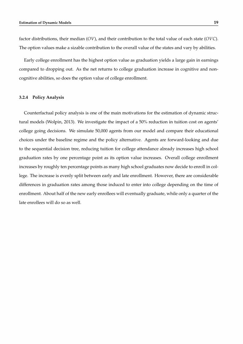
3.2.4 Policy Analysis
Counterfactual policy analysis is one of the main motivations for the estimation of dynamic struc-
tural models (Wolpin, 2013). We investigate the impact of a 50% reduction in tuition cost on agents’
college going decisions. We simulate 50,000 agents from our model and compare their educational
choices under the baseline regime and the policy alternative. Agents are forward-looking and due
to the sequential decision tree, reducing tuition for college attendance already increases high school
graduation rates by one percentage point as its option value increases. Overall college enrollment
increases by roughly ten percentage points as many high school graduates now decide to enroll in col-
lege. The increase is evenly split between early and late enrollment. However, there are considerable
differences in graduation rates among those induced to enter into college depending on the time of
enrollment. About half of the new early enrollees will eventually graduate, while only a quarter of the
late enrollees will do so as well.

Estimation of Dynamic Models 20
Figure 3: Transition Probabilities by Abilities
Cognitive Skills
12
34
56
78
910
Non-cognitive Skills 12
34
56
78910
Prob
abili
ty
0.0
0.2
0.4
0.6
0.8
1.0
(a) High School Finishing
Cognitive Skills
12
34
56
78
910
Non-cognitive Skills 12
34
56
78910
Prob
abili
ty
0.0
0.2
0.4
0.6
0.8
1.0
(b) Early College Enrollment
Cognitive Skills
12
34
56
78
910
Non-cognitive Skills 12
34
56
78910
Prob
abili
ty
0.0
0.2
0.4
0.6
0.8
1.0
(c) Early College Graduation
Cognitive Skills
12
34
56
78
910
Non-cognitive Skills 12
34
56
78910
Prob
abili
ty
0.0
0.2
0.4
0.6
0.8
1.0
(d) Late College Enrollment
Cognitive Skills
12
34
56
78
910
Non-cognitive Skills 12
34
56
78910
Prob
abili
ty
0.0
0.2
0.4
0.6
0.8
1.0
(e) Late College Graduation
Notes: We simulate a sample of 50,000 agents based on the estimates of the model. In each subfigure, we condition on theagents that actually visit the relevant decision state.

Estimation of Dynamic Models 21
Figure 4: Ex Ante Net Returns by Abilities
Cognitive Skills
12
34
56
78
910
Non-cognitive Skills 12
34
56
78910
Net
Ret
urn
-0.4-0.20.00.20.40.60.8
1.0
1.2
1.4
(a)High School Finishing
NRa = 0.64GRa = 0.27
Cognitive Skills
12
34
56
78
910
Non-cognitive Skills 12
34
56
78910
Net
Ret
urn
-0.5-0.4-0.3-0.2-0.10.00.1
0.2
0.3
0.4
(b)Early College Enrollment
NRa = -0.03GRa = 0.14
Cognitive Skills
12
34
56
78
910
Non-cognitive Skills 12
34
56
78910
Net
Ret
urn
-0.4-0.20.00.20.40.60.8
1.0
1.2
1.4
(c)Early College Graduation
NRa = 0.50GRa = 0.75
Cognitive Skills
12
34
56
78
910
Non-cognitive Skills 12
34
56
78910
Net
Ret
urn
-1.0
-0.8
-0.6
-0.4
-0.2
0.0
0.2
(d)Late College Enrollment
NRa = -0.21GRa = 0.29
Cognitive Skills
12
34
56
78
910
Non-cognitive Skills 12
34
56
78910
Net
Ret
urn
-0.8-0.6-0.4-0.20.00.20.4
0.6
0.8
1.0
(e)Late College Graduation
NRa = 0.10GRa = 0.24
Notes: We simulate a sample of 50,000 agents based on the estimates of the model. In each subfigure, we condition on theagents that actually visit the relevant decision state.

Estimation of Dynamic Models 22
Figure 5: Option Values by Abilities
Cognitive Skills
12
34
56
78
910
Non-cognitive Skills 12
34
56
78910
Opt
ion
Val
ue
0.0
0.5
1.0
1.5
2.0
2.5
3.0
3.5
4.0
(a)High School Finishing
OV = 0.52OVC = 0.07
Cognitive Skills
12
34
56
78
910
Non-cognitive Skills 12
34
56
78910
Opt
ion
Val
ue
0.0
1.0
2.0
3.0
4.0
5.0
6.0
7.0
8.0
(b)Early College Enrollment
OV = 3.06OVC = 0.30
Cognitive Skills
12
34
56
78
910
Non-cognitive Skills 12
34
56
78910
Opt
ion
Val
ue
0.0
1.0
2.0
3.0
4.0
5.0
6.0
(c)Late College Enrollment
OV = 1.87OVC = 0.17
Notes: We simulate a sample of 50,000 agents based on the estimates of the model. In each subfigure, we condition on theagents that actually visit the relevant decision state. In units of $100,000.

Estimation of Dynamic Models 23
4 Comparison of ML and SMM
We use the baseline estimates of our structural parameters to simulate a synthetic sample of 5,000
agents. This sample captures important aspects of our original data such as model complexity and
sizable unobserved variation in agent behaviors. We disregard our knowledge about the true struc-
tural parameters and estimate the model on the synthetic sample by ML and SMM to compare their
performance in recovering the true structural objects. We first describe the implementation of both
estimation procedures. Then we compare their within-sample model fit and assess the accuracy of
the estimated returns to education and policy predictions. Finally, we explore the sensitivity of our
SMM results to alternative tuning parameters such as choice of the moments, number of replications,
weighting matrix, and optimization algorithm.
We assume the same functional forms and distributions of unobservables for ML and SMM. Mea-
surement, outcome, and cost equations (1) - (3) are linear-in-parameters. Recall that Sc denotes the
subset of states with a costly exit.
M(j) = X(j)′κj + θ′γj + ν(j) ∀ j ∈ M
Y(s) = X(s)′βs + θ′αs + ε(s) ∀ s ∈ SC(s′, s) = Q(s′, s)′δs′,s + θ′ϕs′,s + η(s′, s) ∀ s ∈ S c
All unobservables of the model are normally distributed:
η(s′, s) ∼ N (0, ση(s′,s)) ∀ s ∈ S c ε(s) ∼ N (0, σε(s)) ∀ s ∈ Sθ ∼ N (0, σθ) ∀ θ ∈ Θ ν(j) ∼ N (0, σν(j)) ∀ j ∈ M.
The unobservables (ε(s), η(s′, s), ν(j)) are independent across states and measures. The two factors θ
are independently distributed. This still allows for unobservable correlations in outcomes and choices
through the factor components θ (Cunha et al., 2005).
4.1 The ML Approach
We now describe the likelihood function, its implementation, and the optimization procedure.

Estimation of Dynamic Models 24
For each agent we define an indicator function G(s) that takes value one if the agent visits state s.
Let ψ ∈ Ψ denote a vector of structural parameters and Γ the subset of states visited by agent i. We
collect in D =X(j)j∈M, X(s), Q(s′, s)s∈S
all observed agent characteristics. Then the likelihood
for observation i is given by∫Θ
∏j∈M
f(
M(j)∣∣∣ D, θ; ψ
)︸ ︷︷ ︸
Measurement
∏s∈S
f(
Y(s)∣∣∣ D, θ; ψ
)︸ ︷︷ ︸
Outcome
Pr(
G(s) = 1∣∣∣ D, θ; ψ
)︸ ︷︷ ︸
Transition
1s∈Γ dF(θ), (10)
where Θ is the support of θ. After taking the logarithm of equation (10) and summing across all agents,
we obtain the sample log likelihood.
Let φσ(·) denote the probability density function and Φσ(·) the cumulative distribution function of
a normal distribution with mean zero and variance σ. The density functions for measurement and
earning equations take a standard form conditional on the factors and other relevant observables:
f(
M(j) | θ, X(j))
= φσν(j)
(M(j)− X(j)′κj − θ′γj
)∀ j ∈ M
f(
Y(s) | θ, X(s))
= φσε(s)
(Y(s)− X(s)′βs − θ′αs
)∀ s ∈ S .
The derivation of the transition probabilities has to account for forward-looking agents who make
their educational choices based on the current costs and expectations of future rewards. Agents
know the full cost of the next transition and the systematic parts of all future earnings and costs
(X(s)′βs, Q(s′, s)′δs′,s). They do not know the values of future random shocks. Agents at state s decide
whether to transition to the costly state s′ or the no-cost alternative s′. Their ex ante valuations T(s′) in-
corporate expected earnings and costs, and the continuation value CV(s′) from future opportunities.
Given our functional form assumptions, the ex ante value of state s′ is:
T(s′) =
X′(s′)βs′ + θ′αs′ −Q(s′, s)′δs′,s − θ′ϕs′,s + CV(s′) if s′ = s′
X′(s′)βs′ + θ′αs′ + CV(s′) if s′ = s′.

Estimation of Dynamic Models 25
The ex ante state evaluations and distributional assumptions characterize the transition probabilities:
Pr(
G(s′) = 1∣∣∣ D, θ; ψ
)=
Φση(s′ ,s) (T(s
′)− T(s′)) if s′ = s′
1−Φση(s′ ,s) (T(s′)− T(s′)) if s′ = s′.
Finally, the continuation value of s is:
CV(s) =[Φση(s′ ,s)
(T(s′)− T(s′)
)]×∫ T(s′)−T(s′)
−∞
[T(s′)− η
] φση(s′ ,s)(η)
Φση(s′ ,s)(T(s′)− T(s′))
dη
+[1−Φση(s′ ,s)
(T(s′)− T(s′)
)]× T(s′),
where we integrate over the conditional distribution of η(s′, s) as the agent chooses the costly transi-
tion to s′ only if T(s′)− η(s′, s) > T(s′).
We compare ML against SMM for statistical and numerical reasons. ML estimation is fully efficient
as it achieves the Cramér-Rao lower bound. The numerical precision of the overall likelihood function
is very high with accuracy up to 15 decimal places. This guarantees at least three digits of accuracy for
all estimated model parameters. We discuss the numerical properties of the likelihood and bounds on
approximation error in Web Appendix D and E. We use Gaussian quadrature to evaluate the integrals
of the model.14 We maximize the sample log likelihood using the Broyden-Fletcher-Goldfarb-Shanno
(BFGS) algorithm (Press et al., 1992).
4.2 The SMM Approach
We present the basic idea of the SMM approach and the details of the criterion function. Then we
discuss the choice of tuning parameters. The goal in the SMM approach is to choose a set of structural
parameters ψ to minimize the weighted distance between selected moments from the observed sample
14See Judd and Skrainka (2011) for a comparison of alternative integration strategies.

Estimation of Dynamic Models 26
and a sample simulated from a structural model. The criterion function takes the following form:
Λ(ψ) =[
f − f (ψ)]′
W−1[
f − f (ψ)]
, (11)
where f represents a vector of moments computed on the observed data and f (ψ) denotes an average
vector of moments calculated from R simulated datasets and W is a positive definite weighting matrix.
We define f (ψ) as:
f (ψ) =1R
R
∑r=1
fr(ur; ψ).
The simulation of the model involves the repeated sampling of the unobserved components ur =
ε(s), η(s′, s)s∈S determining agents’ outcomes and choices. We repeat the simulation R times for
fixed ψ to obtain an average vector of moments. fr(ur; ψ) is the set of moments from a single simulated
sample. We solve the model through backward induction and simulate 5,000 educational careers to
compute each single set of moments. We keep the conditioning on exogenous agent characteristics
implicit in equation (11).
We account for θ by estimating a vector of factor scores based on M that proxy the latent skills
for each participant (Bartlett, 1937). The scores are subsequently treated as ordinary regressors in the
estimation of the auxiliary models. We use the true factors in the simulation steps, assuring that SMM
and ML are correctly specified.
The random components ur are drawn at the beginning of the estimation procedure and remain
fixed throughout. This avoids chatter in the simulation for alternative ψ, where changes in the criterion
function could be due to either ψ or ur (McFadden, 1989).
To implement our criterion function it is necessary to choose a set of moments, the number of repli-
cations, a weighting matrix, and an optimization algorithm. Later, we investigate the sensitivity of
our results to these choices.
We select our set of moments in the spirit of the efficient method of moments (EMM), which pro-
vides a systematic approach to generate moment conditions for the generalized method of moments
(GMM) estimator (Gallant and Tauchen, 1996). Gallant and Tauchen (1996) propose using the expec-

Estimation of Dynamic Models 27
tation under the structural model of the score from an auxiliary model as the vector of moment condi-
tions. We do not directly implement EMM but follow a Wald approach instead, as we do not minimize
the score of an auxiliary model but a quadratic form in the difference between the moments on the sim-
ulated and observed data. Nevertheless, we draw on the recent work by Heckman et al. (2014b) as
an auxiliary model to motivate our moment choice.15 Heckman et al. (2014b) develop a sequential
schooling model that is a halfway house between a reduced form treatment effect model and a fully
formulated dynamic discrete choice model such as ours. They approximate the underlying dynamics
of the agents’ schooling decisions by including observable determinants of future benefits and costs
as regressors in current choice. We follow their example and specify these dynamic versions of Linear
Probability (LP) models for each transition. In addition, we include mean and standard deviation of
within state earnings and the parameters of Ordinary Least Squares (OLS) regressions of earnings on
covariates to capture the within state benefits to educational choices. We add state frequencies as well.
Overall, we start with a total 440 moments to estimate 138 free structural parameters.
We set the number of replications R to 30 and thus simulate a total of 150,000 educational careers
for each evaluation of the criterion function. The weighting matrix W is a matrix with the variances of
the moments on the diagonal and zero otherwise. We determine the latter by resampling the observed
data 200 times. We exploit that our criterion function has the form of a standard nonlinear least-
squares problem in our optimization. Due to our choice of the weighting matrix, we can rewrite
15If the weighting matrices are appropriately chosen and the auxiliary model is correctly speci-
fied, then both approaches are asymptotically equivalent to ML (Gouriéroux et al., 1993). The EMM
approach requires analytical derivatives for the auxiliary model, which is a very time-consuming,
error-prone, and tedious task for large and complex models. For this reason, the EMM approach is
not commonly used to estimate dynamic discrete choice models, but widely applied to fit stochastic
volatility models. In the latter case, several tractable auxiliary models such as ARCH and GARCH are
readily available (Andersen et al., 1999). See Carrasco and Florens (2002) for an accessible comparison
of EMM to other simulation-based methods and additional references.

Estimation of Dynamic Models 28
equation (11) as:
Λ(ψ) =
I
∑i=1
(fi − fi(ψ)
σi
)2
,
where I is the total number of moments, fi denotes moment i, and σi its bootstrapped standard devia-
tion.
Our criterion is not a smooth function of the model parameters. Small changes in the structural
parameters cause some simulated agents to change their educational choices, resulting in discrete
jumps in our set of moments (Keane and Smith, 2003). Thus we cannot use gradient-based methods for
optimization and rely on derivative-free alternatives instead. Moré and Wild (2009) show that model-
based solvers perform better than standard derivative-free direct search solvers used in the existing
literature (see Adda et al. (2013, 2011) and Del Boca et al. (2014) for applications of derivative-free
direct search solvers). From the class of model-based solvers, we choose the Practical Optimization
Using No Derivatives for Sums of Squares (POUNDerS) algorithm (Munson et al., 2012). POUNDerS
exploits the special structure of the nonlinear least-squares problem within a derivative-free trust-
region framework and forms a smooth approximation model of the objective function to converge to
a minimum.16
4.3 Results
We compare ML and SMM estimation to learn whether our version of SMM is a good substitute
for ML. First, we compare basic model fit statistics. Second, we study the estimates for the returns to
education and perform a counterfactual policy exercise. Finally, we explore alternative choices for the
set of moments, weighting matrix, number of replications, and optimization algorithm.
16See Nocedal and Wright (2006) for a discussion of the nonlinear least-squares problem and Korte-
lainen et al. (2010) for a detailed description of the underlying mechanics of POUNDerS.

Estimation of Dynamic Models 29
Model Fit Table 4 shows the average annual earnings for each state and the conditional state fre-
quencies. Overall, both estimation approaches fit these aggregate statistics quite well. The model fit
for the average earnings among late college graduates and late college dropouts is slightly worse than
for the other states as the agent count in those states is low. This affects the SMM estimates more than
ML. The state frequencies are matched very well in both cases.
We report the root-mean-square error (RMSE) based on the difference between the simulated and
observed statistics. There are only minor discrepancies for both estimation approaches. Nevertheless,
they are slightly smaller for the ML results.
Table 4: Cross Section Model Fit
Average Earnings State Frequencies
State Observed ML SMM Observed ML SMM
High School Finishing 0.78 0.76 0.78 0.86 0.84 0.86
High School Dropout 2.50 2.53 2.54 0.14 0.16 0.14
Early College Enrollment 1.45 1.42 1.45 0.41 0.41 0.41
High School Graduation 2.46 2.44 2.45 0.45 0.43 0.45
Early College Graduation 6.81 6.99 6.67 0.29 0.30 0.29
Early College Dropout 3.91 3.97 4.02 0.12 0.11 0.12
Late College Enrollment 2.51 2.55 2.52 0.13 0.13 0.13
High School Graduation (cont’d) 3.88 3.83 3.79 0.32 0.30 0.32
Late College Graduation 6.03 6.21 6.19 0.07 0.07 0.07
Late College Dropout 5.10 4.89 5.05 0.06 0.06 0.06
ML SMM
RMSE 0.05058 0.05748
Notes: Earnings are discounted using the within state duration and measured in units of $10,000. Statistics calculated
for ML and SMM approaches based on 50,000 simulated agents using the parameter estimates. RMSE = root-mean-
square error.
We apply χ2 goodness of fit tests (Heckman, 1984; Heckman and Walker, 1990) to the estimated and

Estimation of Dynamic Models 30
actual probabilities. In Table 5 we report the p-value of a joint test of the relative share of agents within
each state conditional on all possible realizations of selected covariates.17
Table 5: Conditional Model Fit
State Number of Children Baby in Household Parental Education Broken Home
SMM ML SMM ML SMM ML SMM ML
High School Dropout 0.90 0.75 0.83 0.95 0.26 0.56 0.65 0.62
High School Finishing 0.99 0.99 0.99 0.99 0.96 0.99 0.97 0.89
High School Graduation 0.84 0.72 0.99 0.99 0.86 0.99 0.40 0.50
High School Graduation (cont’d) 0.67 0.90 0.98 0.98 0.90 0.98 0.37 0.42
Early College Enrollment 0.04 0.49 0.98 0.97 0.87 0.94 0.39 0.58
Early College Graduation 0.63 0.91 0.81 0.86 0.07 0.06 0.89 0.58
Early College Dropout 0.42 0.72 0.99 0.99 0.86 0.99 0.40 0.50
Late College Enrollment 0.27 0.62 0.99 0.94 0.14 0.25 0.84 0.96
Late College Graduation 0.56 0.11 0.97 0.99 0.07 0.06 0.72 0.97
Late College Dropout 0.71 0.77 0.62 0.17 0.08 0.89 0.45 0.89
Overall, the level of p-values is high. For ML estimation, all p-values indicate that our model is con-
sistent with the data at the 5% significance level. In the case of SMM, we only do not pass the test con-
ditional on Number of Children among early college enrollees. Because tests within covariates across all
states are not independent, we use a Bonferroni test to evaluate the joint hypothesis that the predicted
covariate distributions fit at each state. The test is based on the maximum χ2 statistic over all states
for each covariate. We pass a 5% Bonferroni test for all covariates and both estimation approaches.
Economic Implications Table 6 presents the median ex ante gross returns GRa(s′, s′, s) and net re-
turns NRa(s′, s′, s) of pursuing a higher education by transitioning from s to s′. Both capture all current
and future earnings. However, they differ with regards to current and future costs. Their systematic
parts are included in the calculation of the NRa(s′, s′, s) but not the GRa(s′, s′, s) as we discussed in
17In the χ2 test, the predicted conditional distributions depends on estimated parameters. We do
not adjust the test statistic to account for parameter estimation error as suggested by Heckman (1984)
because the adjustments are usually slight (Heckman and Walker, 1990).

Estimation of Dynamic Models 31
Section 2.2.
Table 6: Economic Implications
Gross Return Net Return
State True ML SMM True ML SMM
High School Finishing 28% 35% 33% 66% 62% 138%
Early College Enrollment 14% 18% 18% -2% -1% -4%
Early College Graduation 71% 75% 61% 48% 48% 93%
Late College Enrollment 28% 30% 29% -23% -21% -58%
Late College Graduation 22% 22% 16% 9% 6% 24%
ML SMM
RMSE 0.03416 0.29775
Notes: Statistics calculated for ML and SMM approaches based on 50,000 simulated agents using the
parameter estimates. RMSE = root-mean-square error calculated in units of 100%.
The estimates for the gross returns GRa(s′, s′, s) are very similar for the two approaches and close to
their true values. However, for the net returns NRa(s′, s′, s) only the ML results are close to the truth.
The SMM results are off by up to a factor of two. For example, the true net return of finishing high
school is 66%, while SMM estimates 138%. The RMSE is roughly one order of magnitude larger for
SMM than ML estimation. This difference is solely driven by the discrepancies in the net returns.
Table 7 sheds light on the poor performance of our SMM approach in the estimation of the net
returns. These, in contrast to the gross returns, include the current costs and the systematic part of
all future costs of educational choices. SMM is unable to detect the systematic differences in the cost
faced by agents. We overestimate the variance of the unobserved component determining choices
ση(s′ ,s) . Too much of the agents’ decisions is attributed to random cost shocks and not their systematic
differences. This translates into an excess net return as we underestimate the cost associated with
future educational choices. Despite encouraging values for model fit criteria, SMM fails to accurately
estimate the net return to educational choices.

Estimation of Dynamic Models 32
Table 7: Standard Deviations
ση(s′ ,s)
State True ML SMM
High School Finishing 0.27 0.24 0.61
Early College Enrollment 0.20 0.19 0.47
Early College Graduation 0.61 0.60 1.30
Late College Enrollment 0.22 0.20 0.56
Late College Graduation 0.61 0.60 1.30
RMSE 0.016 0.496
Notes: RMSE = root-mean-square error.
We also explore the impact of a 50% reduction in tuition cost on agents’ college going decisions.
We simulate 50,000 agents from our model and compare their educational choices under the baseline
regime and the policy alternative using the results from the two estimation approaches. Based on
the ML results, all policy predictions line up with the underlying truth. This is only partly true for
the SMM estimation, where the predicted graduation rate for those induced to enroll in college late
is too optimistic. Only a quarter will actually graduate, while the SMM results forecast about half.
The SMM’s failure to distinguish between the systematic and unsystematic cost components driving
educational choices translates into (partly) flawed policy conclusions as well.
We now investigate the poor performance of our application of SMM and start with some evidence
that we indeed recover a global minimum of our criterion function. Figure 6 shows the value of Λ(ψ)
around our SMM estimates as we perturb all parameters in a random direction in t increments. All
perturbations increase the discrepancies between the observed and simulated sample. However, Λ(ψ)
is not zero because of remaining differences between estimated and true structural parameters. Even
if we set ψ = ψ∗, then Λ(ψ∗) evaluates at 434 (horizontal dashed line) due to the random variation
in agents’ behaviors and state experiences. The moments provide noisy information about the data
generating process due to the random components. The more variation due to unobservables, the less
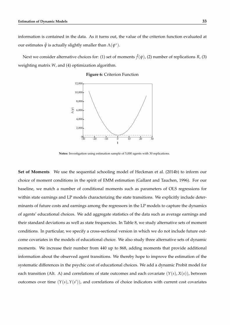
Estimation of Dynamic Models 33
information is contained in the data. As it turns out, the value of the criterion function evaluated at
our estimates ψ is actually slightly smaller than Λ(ψ∗).
Next we consider alternative choices for: (1) set of moments f (ψ), (2) number of replications R, (3)
weighting matrix W, and (4) optimization algorithm.
Figure 6: Criterion Function
-30 -20 -10 0 10 20 30t
0
2,000
4,000
6,000
8,000
10,000
12,000
Λ(ψ
)
Notes: Investigation using estimation sample of 5,000 agents with 30 replications.
Set of Moments We use the sequential schooling model of Heckman et al. (2014b) to inform our
choice of moment conditions in the spirit of EMM estimation (Gallant and Tauchen, 1996). For our
baseline, we match a number of conditional moments such as parameters of OLS regressions for
within state earnings and LP models characterizing the state transitions. We explicitly include deter-
minants of future costs and earnings among the regressors in the LP models to capture the dynamics
of agents’ educational choices. We add aggregate statistics of the data such as average earnings and
their standard deviations as well as state frequencies. In Table 8, we study alternative sets of moment
conditions. In particular, we specify a cross-sectional version in which we do not include future out-
come covariates in the models of educational choice. We also study three alternative sets of dynamic
moments. We increase their number from 440 up to 868, adding moments that provide additional
information about the observed agent transitions. We thereby hope to improve the estimation of the
systematic differences in the psychic cost of educational choices. We add a dynamic Probit model for
each transition (Alt. A) and correlations of state outcomes and each covariate (Y(s), X(s)), between
outcomes over time (Y(s), Y(s′)), and correlations of choice indicators with current cost covariates

Estimation of Dynamic Models 34
(G(s′), Q(s′, s)) (Alt. B).
Table 8: Set of Moments
Cross Section Moments Dynamic (Panel) Moments
Sets Base Base Alt. A Alt. B
Outcome Models
Means X X X X
Standard Deviations X X X X
Ordinary Least Squares X X X X
Correlations X
Choice Models
State Frequencies X X X X
Linear Probability
- cross section X
- dynamic X X X
Probit
- dynamic X X
Correlations X
Overall Statistics
Number of Moments 222 440 690 868
Number of Replications 50 50 50 50
Weighting Matrix diagonal variance matrix
Algorithm POUNDerS
Quality of Fit Measures
Λ(ψ) 130.69 383.49 666.57 798.33
Λ(ψ∗) 222.12 434.07 685.94 847.64
Notes: Alt. = Alternative.

Estimation of Dynamic Models 35
We also report the value of the criterion function at the true structural parameters Λ(ψ∗). Its difference
from zero is solely driven by the presence of the random disturbances ur. The final values of our
criterion function are always below Λ(ψ∗) which gives us further confidence that we attained a global
minimum in those cases.
We show the implications of alternative moments for the estimated median ex ante gross and net
returns to education in Table 9.
Table 9: Robustness of Economic Implications of Alternative Implementations of SMM
Cross Section Moments Dynamic (Panel) Moments
State True Base Base Alt. A Alt. B
Gross Return
High School Finishing 28% 38% 33% 34% 35%
Early College Enrollment 14% 18% 18% 19% 19%
Early College Graduation 71% 74% 61% 67% 61%
Late College Enrollment 28% 17% 29% 25% 26%
Late College Graduation 22% 18% 16% 19% 14%
Net Return
High School Finishing 66% 154% 138% 137% 137%
Early College Enrollment -2% -4% -4% -4% -4%
Early College Graduation 48% 89% 93% 94% 93%
Late College Enrollment -23% -72% -58% -55% -56%
Late College Graduation 9% 16% 24% 22% 24%
Notes: Statistics calculated for SMM based on 50,000 simulated agents using the parameter estimates.
Once dynamic moments are included in the criterion function, the effect of adding even more is
rather small. The estimates for the gross and net returns are all very similar. However, when using

Estimation of Dynamic Models 36
only cross-sectional moments for the criterion function, the performance of SMM deteriorates and its
ability to recover the net returns is undermined further.
We assess the information content of selected moments fi and investigate the effect of perturba-
tions around ψ. In Figure 7, we perturb the intercept in the structural earnings equation for early
college graduates in t increments. This has a direct effect on average earnings in that state (Figure 7a).
However, agents are forward-looking and these changes also affect moments associated with earlier
decisions such as finishing high school (Figure 7b). This is true even though the immediate benefits of
doing so (Figure 7c) are unaffected. Agents change their early educational choices due to the increase
in the option value of finishing high school, which includes the expected future value of potentially
graduating from college.
Figure 7: Parameter Perturbations, Outcome
-40 -20 0 20 40t
0.04
0.05
0.06
0.07
0.08
0.09
f i
(a) College Graduation, Average Earnings
-40 -20 0 20 40t
0.84
0.85
0.86
0.87
0.88
f i
(b) High School Finishing, State Frequency
-40 -20 0 20 40t
0.007
0.008
0.009
f i
(c) High School Finishing, Average Earnings

Estimation of Dynamic Models 37
Number of Replications For a given set of structural parameters, we create multiple simulated
datasets from which we calculate the moments. Averaging over those moments, we reduce the effect
of random components determining agents’ choices and state experiences. In Figure 8 we show the
value of the criterion function at the true structural parameters ψ∗ for different numbers of replications
R. The difference from zero is solely driven by the random components determining agents’ choices
and outcomes. If the model is simulated only once, then Λ(ψ∗) takes value 825. Initially, increases
in R result in a large drop of Λ(ψ∗). However, this effect levels off after more than 20 replications.
Afterwards, the value of Λ(ψ∗) oscillates around 435. In a finite sample, differences between f and
f (ψ∗) remain even for a very large number of replications. While the random values of (ε(s), η(s′, s))
wash out in the simulated moments, their particular realizations remain relevant in the finite observed
data.18 For our baseline estimates we set R = 30. Further increases do not change model fit or eco-
nomic implications.
Figure 8: Role of Replications
0 20 40 60 80 100R
400
450
500
550
600
650
700
750
800
850
Λ(ψ∗ )
Notes: Investigation using estimation sample of 5,000 agents with varying number of replications.
Weighting Matrix Our optimization algorithm is only guaranteed to converge to local minimizers.
Figure 9 plots the surface of our criterion function around ψ∗ for two alternative choices of W given
the true values of ur. Thus, f = f (ψ∗) and Λ(ψ∗) evaluates initially to zero regardless of the weighting
18See Kristensen and Salanié (2011) for a comprehensive statistical analysis of estimation methods,
where the objective function is approximated through simulation or discretization.

Estimation of Dynamic Models 38
matrix used. Then we perturb all the structural parameters in a random direction in t increments. We
show the surface of Λ(ψ) when either the identity matrix (Figure 9a) or the diagonal matrix with the
variances of the moments (Figure 9b) is used. Choosing the identity matrix for W results in multiple
local minima, whereas using the variances smoothes the overall surface of the criterion function.
Figure 9: Alternative Weighting Matrices
0 10 20 30 40 50t
0
1,000
2,000
3,000
4,000
5,000
Λ(ψ
)
(a) Identity Matrix
0 10 20 30 40 50t
0
20
40
60
80
100
Λ(ψ
)
(b) Inverse Variances on Diagonal
Notes: Investigation using estimation sample of 5,000 agents with one replication and alternative weighting matrices.
Optimization Algorithm Because we repeat the SMM estimation many times for our Monte Carlo
study, we benefit from a fast optimization algorithm. In Figure 10 we compare the performance of
POUNDerS to the standard Nelder-Mead algorithm (Nelder and Mead, 1965) applied by Del Boca
et al. (2014) and French and Jones (2011) among others. We perturb our estimates ψ and run the two
algorithms as implemented in the Toolkit for Advanced Optimization (TAO) (Munson et al., 2012) to
investigate their relative performance. Following Moré and Wild (2009) the solvers are tested using
their default options.19 Both algorithms are derivative-free, but differ in their search strategy and how
they exploit the structure of the criterion function. Nelder-Mead applies a direct search method, while
19We are aware that performance can change for other choices. However, our practical experience
throughout this project lines up with the results from this stylized presentation. We illustrate the rel-
ative performance of the two algorithms using a single processor only. Both algorithms allow parallel
implementations as well (Lee and Wiswall, 2007; Munson et al., 2012).

Estimation of Dynamic Models 39
POUNDerS forms an approximation model within a trust region which exploits the special structure
of our nonlinear least-squares problem. We show a minute-by minute account of the criterion function
Λ(ψ) over five hours.
Figure 10: Optimization Algorithms
0 50 100 150 200 250 300CPU Minutes
0
500
1,000
1,500
2,000
2,500
3,000
Λ(ψ
)
Nelder-Mead POUNDerS
Notes: Investigation using estimation sample of 5,000 agentswith 30 replications and all tuning parameters of the algo-rithms set to their default values.
The POUNDerS algorithm attains a lower bound of Λ(ψ) ≈ 385 after about two and a half hours and
terminates. With the Nelder-Mead algorithm, the criterion function still takes a value of Λ(ψ) ≈ 2, 050
after five hours. Even after 36 hours, the Nelder-Mead solution Λ(ψ) ≈ 1, 126 is still about three times
as large as the POUNDerS solution.
We are unable to improve the SMM results by using alternative tuning parameters. Our discus-
sion cautions that inspection of model fit statistics alone does not guarantee accurate economic im-
plications. For our model, large unobserved variation in educational choices translates into a noisy
criterion function, which leaves SMM unable to recover the true returns to education. The structural
variances of the unobserved cost shocks are poorly estimated; we are unable to correctly distinguish
between the systematic and unsystematic cost components of educational choices.
Our results do not discredit SMM as a useful tool for the estimation of complex economic models.
Our results are highly model dependent, but our diagnostics are not. We now outline a Monte Carlo
exercise that allows SMM users to build confidence in their particular implementation in any applied
Estimation of Dynamic Models 40
setting.
Monte Carlo Exercise to Gain Confidence in an SMM Algorithm. LetM(ψ) denote the structural
model parametrized by ψ which is fit to the observed data Dobs to produce an estimated set of param-
eters ψobs using SMM.
Step 1 Simulate a synthetic sample Dsyn fromM(ψobs) using the estimated results.
Step 2 FitM(ψ) on the synthetic sample Dsyn using SMM to produce ψsyn.
Step 3 Compare ψobs to the results from the synthetic sample ψsyn.
Using the initial estimates as the parametrization for the Monte Carlo exercise ensures that important
features of the data generating process, in our case the large unobserved variability in agent behaviors,
are accounted for. In Step 2, it is crucial to follow the same estimation approach applied to the original
data as closely as possible, e.g. choice of starting values. Combining the application of fast state of the
art optimization algorithms with parallel computing allows for such an analysis even in computation-
intensive models.
This exercise showcases the performance of the estimator in a favorable setting as the model is
correctly specified. If the structural parameters ψsyn are successfully recovered, this is encouraging but
does not provide a definite proof of the performance in the observed data. A failure, however, offers
reason for concern. The algorithm might be improved, for example, by varying the set of moments
used to test SMM.
5 Conclusion
We compare the performance of simulated method of moments (SMM) and maximum likelihood
(ML) estimation in dynamic discrete choice models. We estimate a simplified dynamic model of ed-
ucational choices which emphasizes the role of unobserved heterogeneity, psychic costs, and option
values for the net returns to schooling. The primary value of the model comes as input to the simula-
tion study that is the core of this paper.

Estimation of Dynamic Models 41
We estimate our model on a sample of white males from the National Longitudinal Survey of Youth
of 1979 (NLSY79). We discuss its implications for schooling decisions and present estimates of option
values by cognitive and non-cognitive factors. Given our estimates, we simulate a synthetic sample,
creating a realistic setting to compare ML and SMM estimation. Our model allows for ML estimation
without the need for any simulation in the likelihood function, which provides a clean comparison of
ML against simulation-based estimation methods such as SMM. ML and SMM pass standard model fit
tests. However, while the ML estimates are close to the true structural objects of interest, our version
of SMM fails to recover the true net returns to education and policy effects. The SMM is unable to
distinguish between systematic and unsystematic cost components driving educational choices.
We investigate alternative tuning parameters for implementing our SMM procedure. We specify
alternative sets of moment conditions and show how the benefit of additional moments depends on
the unique information they provide. Moments that capture the dynamics of agent behavior are crucial
for getting reliable estimates of dynamic models. A large replication count in the simulation step
reduces the effect of random noise in the measurement of the criterion function. An appropriate choice
of the weighting matrix smoothes the surface of the criterion function and reduces the risk of local
minima. Based on our analysis, we recommend that more exacting model specification tests and
Monte Carlo evidence be provided to verify the performance of SMM in any application.

Estimation of Dynamic Models 42
References
ABBOTT, B., G. GALLIPOLI, C. MEGHIR AND G. L. VIOLANTE, “Education Policy and Intergener-
ational Transfers in Equilibrium,” Working Paper 18782, National Bureau of Economic Research,
February 2013.
ADDA, J., C. DUSTMANN, C. MEGHIR AND J.-M. ROBIN, “Career Progression, Economic Downturns,
and Skills,” Working Paper 18832, National Bureau of Economic Research, February 2013.
ADDA, J., C. DUSTMANN AND K. STEVENS, “The Career Costs of Children,” Working Paper 6201,
Institute for the Study of Labor, December 2011.
ANDERSEN, T. G., L. BENZONI AND J. LUND, “An Empirical Investigation of Continuous-Time Equity
Return Models,” Journal of Finance 57 (December 2002), 1239–1284.
ANDERSEN, T. G., H.-J. CHUNG AND B. E. SORENSEN, “Efficient Method of Moments Estimation of
a Stochastic Volatility Model: A Monte Carlo Study,” Journal of Econometrics 91 (July 1999), 61–87.
ARCIDIACONO, P. AND R. A. MILLER, “Conditional Choice Probability Estimation of Dynamic Dis-
crete Choice Models with Unobserved Heterogeneity,” Econometrica 79 (November 2011), 1823–1867.
BARTLETT, M. S., “The Statistical Conception of Mental Factors,” British Journal of Psychology 1 (July
1937), 97–104.
BUREAU OF LABOR STATISTICS, NLS Hanbook 2001: The National Longitudinal Surveys (Washington,
DC: U.S. Department of Labor, 2001).
CAMERON, S. V. AND J. J. HECKMAN, “The Nonequivalence of High School Equivalents,” Journal of
Labor Economics 11 (January 1993), 1–47.
CARNEIRO, P., K. HANSEN AND J. J. HECKMAN, “Estimating Distributions of Treatment Effects with
an Application to the Returns to Schooling and Measurement of the Effects of Uncertainty on Col-
lege Choice,” International Economic Review 44 (April 2003), 361–422.
CARRASCO, M. AND J.-P. FLORENS, “Simulation-Based Method of Moments and Efficiency,” Journal
of Business & Economics and Statistics 20 (October 2002), 482–492.
Estimation of Dynamic Models 43
COMAY, Y., A. MELNIK AND M. A. POLLATSCHEK, “The Option Value of Education and the Optimal
Path for Investment in Human Capital,” International Economic Review 14 (June 1973), 421–435.
CUNHA, F., J. J. HECKMAN AND S. NAVARRO, “Separating Uncertainty from Heterogeneity in Life
Cycle Earnings,” Oxford Economic Papers 57 (April 2005), 191–261.
———, “The Identification and Economic Content of Ordered Choice Models with Stochastic Thresh-
olds,” International Economic Review 48 (November 2007), 1273–1309.
CUNHA, F., J. J. HECKMAN AND S. SCHENNACH, “Estimating the Technology of Cognitive and
Noncognitive Skill Formation,” Econometrica 78 (May 2010), 883–931.
DEL BOCA, D., C. FLINN AND M. WISWALL, “Household Choices and Child Development,” Review
of Economic Studies (January 2014), 137–185.
ECKSTEIN, Z. AND K. I. WOLPIN, “The Specification and Estimation of Dynamic Stochastic Discrete
Choice Models: A Survey,” The Journal of Human Resources 24 (Autumn 1989), 562–598.
———, “Why Youths Drop Out of High School: The Impact of Preferences, Opportunities, and Abili-
ties,” Econometrica 67 (November 1999), 1295–1339.
FLINN, C. AND D. DEL BOCA, “Endogenous Household Interaction,” Journal of Econometrics 166 (Jan-
uary 2012), 49–65.
FLINN, C. AND J. MABLI, “On-the-Job Search, Minimum Wages, and Labor Market Outcomes in an
Equilibrium Bargaining Framework,” Working Paper 91, Carlo Alberto Notebooks, December 2008.
FRENCH, E. AND J. B. JONES, “The Effects of Health Insurance and Self-Insurance on Retirement
Behavior,” Econometrica 79 (May 2011), 693–732.
GACH, F. AND B. M. PÖTSCHER, “Nonparametric Maximum Likelihood Density Estimation and
Simulation-Based Minimum Distance Estimators,” Mathematical Methods of Statistics 20 (December
2011), 288–326.
GALLANT, A. R. AND G. TAUCHEN, “Which Moments to Match?,” Econometric Theory 12 (October
1996), 657–681.

Estimation of Dynamic Models 44
GEWEKE, J. F., “Bayesian Inference in Econometric Models using Monte-Carlo Integration,” Economet-
rica 57 (November 1989), 1317–1339.
GOURIÉROUX, C. AND A. MONFORT, Simulation-Based Econometric Methods (New York, NY: Oxford
University Press, 1997).
GOURIÉROUX, C., A. MONFORT AND E. M. RENAULT, “Indirect Inference,” Journal of Applied Econo-
metrics 8 (December 1993), S85–S118.
HAJIVASSILIOU, V. AND D. L. MCFADDEN, “The Method of Simulated Scores for the Estimation of
LDV Models,” Econometrica 66 (July 1998), 863–896.
HANSEN, K., J. J. HECKMAN AND K. MULLEN, “The Effect of Schooling and Ability on Achievement
Test Scores,” Journal of Econometrics 121 (July 2004), 39–89.
HECKMAN, J. J., “Heterogeneity and State Dependence,” in S. Rosen, ed., Studies in Labor Markets
(Chicago, IL: University of Chicago Press, 1981), 91–140.
———, “The χ2 Goodness of Fit Statistic for Models with Parameters Estimated from Microdata,”
Econometrica (November 1984), 1543–1547.
HECKMAN, J. J., J. E. HUMPHRIES AND T. KAUTZ, eds., The Myth of Achievement Tests: The GED and
the Role of Character in American Life (Chicago, IL: University of Chicago Press, 2014a).
HECKMAN, J. J., J. E. HUMPHRIES AND G. VERAMENDI, “Education, Health and Wages,” mimeo, The
University of Chicago, March 2014b.
HECKMAN, J. J., L. J. LOCHNER AND P. E. TODD, “Earnings Functions, Rates of Return and Treatment
Effects: The Mincer Equation and Beyond,” in E. A. Hanushek and F. Welch, eds., Handbook of the
Economics of Educationvolume 1 (Amsterdam, Netherlands: Elsevier, 2006a), 307–458.
HECKMAN, J. J. AND S. NAVARRO, “Dynamic Discrete Choice and Dynamic Treatment Effects,” Jour-
nal of Econometrics 136 (February 2007), 341–396.
HECKMAN, J. J., R. PINTO AND P. A. SAVELYEV, “Understanding the Mechanisms Through Which
an Influential Early Childhood Program Boosted Adult Outcomes,” American Economic Review 103
(October 2013), 2052–2086.

Estimation of Dynamic Models 45
HECKMAN, J. J., J. STIXRUD AND S. URZÚA, “The Effects of Cognitive and Noncognitive Abilities on
Labor Market Outcomes and Social Behavior,” Journal of Labor Economics 24 (July 2006b), 411–482.
HECKMAN, J. J. AND J. R. WALKER, “The Relationship Between Wages and Income and the Timing
and Spacing of Births: Evidence from Swedish Longitudinal Data,” Econometrica 58 (November
1990), 1411–1441.
HOTZ, V. J. AND R. A. MILLER, “Conditional Choice Probabilities and the Estimation of Dynamic
Models,” The Review of Economic Studies 60 (July 1993), 497–529.
JOHNSON, M. T., “Borrowing Constraints, College Enrollment, and Delayed Entry,” Journal of Labor
Economics 31 (October 2013), 669–725.
JUDD, K. L. AND B. SKRAINKA, “High Performance Quadrature Rules: How Numerical Integration
Affects a Popular Model of Product Differentiation,” CeMMAP Working Papers, November 2011.
KEANE, M. AND A. A. SMITH, “Generalized Indirect Inference for Discrete Choice Models,” mimeo,
Yale University, November 2003.
KEANE, M., P. E. TODD AND K. I. WOLPIN, “The Structural Estimation of Behavioral Models: Discrete
Choice Dynamic Programming Methods and Applications,” in O. Ashenfelter and D. Card, eds.,
Handbook of Labor Economicsvolume 4A (Amsterdam, Netherlands: Elsevier, 2011), 331–461.
KEANE, M. AND K. I. WOLPIN, “The Solution and Estimation of Discrete Choice Dynamic Program-
ming Models by Simulation: Monte Carlo Evidence,” Review of Economics and Statistics 76 (Novem-
ber 1994), 648–672.
KEANE, M. P., “A Computationally Practical Simulation Estimator for Panel Data,” Econometrica 62
(January 1994), 95–116.
KEANE, M. P. AND K. I. WOLPIN, “The Career Decisions of Young Men,” Journal of Political Economy
105 (June 1997), 473–522.
———, “The Effects of Parental Transfers and Borrowing Constraints on Education,” International Eco-
nomic Review 42 (November 2001), 1051–1103.

Estimation of Dynamic Models 46
KORTELAINEN, M., T. LESINSKI, J. MORÉ, W. NAZAREWICZ, J. SARICH, N. SCHUNCK, M. V.
STOITSOV AND S. WILD, “Nuclear Energy Density Optimization,” Physical Review C 82 (August
2010), 024313.
KRINSKY, I. AND L. A. ROBB, “On Approximating the Statistical Properties of Elasticities,” The Review
of Economics and Statistics 68 (November 1986), 715–719.
———, “On Approximating the Statistical Properties of Elasticities: A Correction,” The Review of Eco-
nomics and Statistics 72 (Febrary 1990), 189–190.
KRISTENSEN, D. AND B. SALANIÉ, “Higher-order Properties of Approximate Estimators,” mimeo,
Columbia University, June 2011.
LEE, D. AND M. WISWALL, “A Parallel Implementation of the Simplex Function Minimization Rou-
tine,” Computational Economics 30 (September 2007), 171–187.
LEE, D. AND K. I. WOLPIN, “Intersectoral Labor Mobility and the Growth of the Service Sector,”
Econometrica 74 (January 2006), 1–46.
———, “Accounting for Wage and Employment Changes in the U.S. from 1968-2000: A Dynamic
Model of Labor Market Equilibrium,” Journal of Econometrics 156 (May 2010), 68–85.
MCFADDEN, D. L., “A Method of Simulated Moments for Estimation of Discrete Response Models
without Numerical Integration,” Econometrica 57 (September 1989), 995–1026.
MORÉ, J. J. AND S. M. WILD, “Benchmarking Derivative-Free Optimization Algorithms,” SIAM J. Op-
timization 20 (March 2009), 172–191.
MUNSON, T., J. SARICH, S. WILD, S. BENSON AND L. C. MCINNES, “TAO 2.0 Users Manual,” Mathe-
matics and Computer Science Division, Argonne National Laboratory (July 2012).
NELDER, J. A. AND R. MEAD, “A Simplex Method for Function Minimization,” The Computer Journal
4 (January 1965), 308–313.
NICKL, R. AND B. M. PÖTSCHER, “Efficient Simulation-Based Minimum Distance Estimation and
Indirect Inference,” Mathematical Methods of Statistics 19 (December 2010), 327–364.

Estimation of Dynamic Models 47
NOCEDAL, J. AND S. J. WRIGHT, Numerical Optimization (New York, NY: Springer, 2006).
PRESS, W. H., B. P. FLANNERY, S. A. TEUKOLSKY AND W. T. VETTERLING, Numerical Recpies in Fortran
77: The Art of Scientific Computing (New York, NY: Cambridge University Press, 1992).
RAKNERUD, A. AND O. SKARE, “Indirect Inference Methods for Stochastic Volatility Models Based
on Non-Gaussian Ornstein-Uhlenbeck Processes,” Computational Statistics and Data Analysis 56
(November 2012), 3260–3275.
RUGE-MURCIA, F., “Estimating Nonlinear DSGE Models by the Simulated Method of Moments: With
an Application to Business Cycles,” Journal of Economic Dynamics and Control 36 (June 2012), 914–938.
SKRAINKA, B. S., “A Large Scale Study of the Small Sample Performance of Random Coefficient Mod-
els of Demand,” mimeo, The University of Chicago, October 2011.
TRACHTER, N., “Stepping Stone and Option Value in a Model of Postsecondary Education,” Working
Paper 14-03, Federal Reserve Bank of Richmond, February 2014.
WEISBROD, B. A., “Education and Investment in Human Capital,” Journal of Political Economy 70 (Oc-
tober 1962), 106–123.
WOLPIN, K. I., The Limits of Inference Without Theory (Cambridge, MA: MIT Press, 2013).