1

ESTIMATION OF DRIVERS ROUTE CHOICE USING

MULTI-PERIOD MULTINOMIAL CHOICE

MODELS

Stephen Clark and Dr Richard Batley

Institute for Transport StudiesUniversity of Leeds, U.K.

2

Introduction

• Where ‘panel’ data is available on choices made by individuals, it is reasonable to assume that previous experiences somehow condition these choices

3

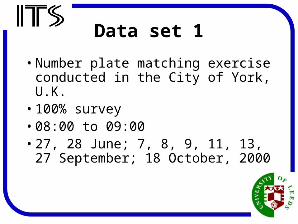
Data set 1

• Number plate matching exercise conducted in the City of York, U.K.

• 100% survey• 08:00 to 09:00 • 27, 28 June; 7, 8, 9, 11, 13, 27

September; 18 October, 2000

4

Repetition and contiguity

• Of the vehicles observed on 2 ‘adjacent’ survey days, over 50% used the same route on both days

• As the period between 2 survey days increased, this percentage dropped– e.g. for 2 survey days 14 working days

apart, the percentage was 35%-40%

5

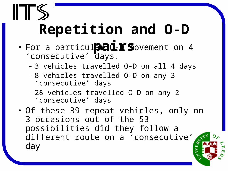
Repetition and O-D pairs• For a particular O-D movement on 4

‘consecutive’ days:– 3 vehicles travelled O-D on all 4 days– 8 vehicles travelled O-D on any 3

‘consecutive’ days– 28 vehicles travelled O-D on any 2

‘consecutive’ days

• Of these 39 repeat vehicles, only on 3 occasions out of the 53 possibilities did they follow a different route on a ‘consecutive’ day

6

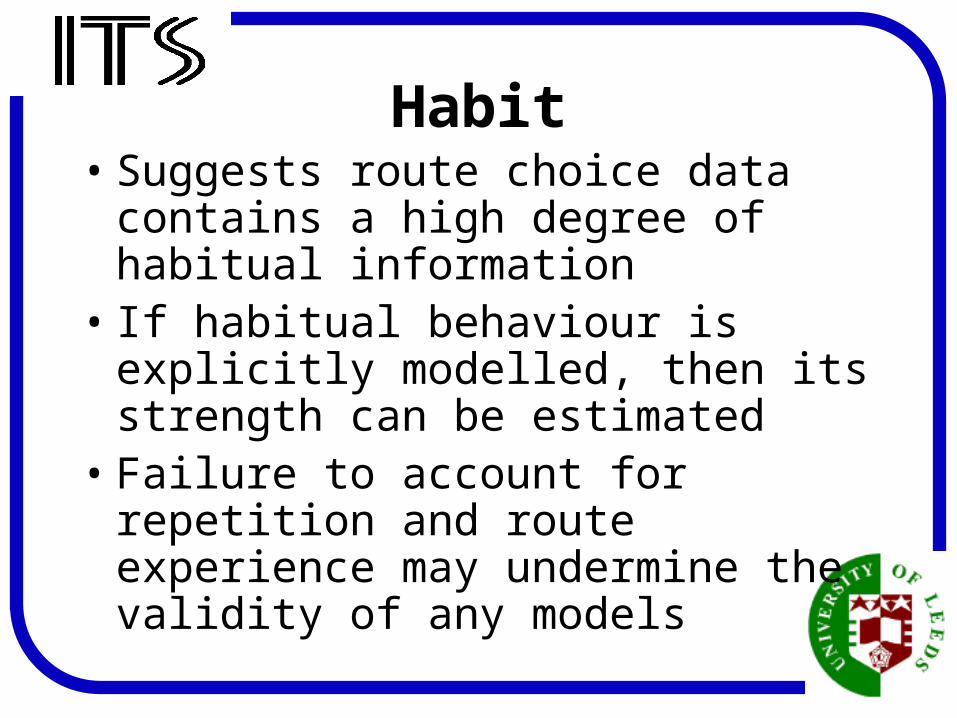
Habit• Suggests route choice data

contains a high degree of habitual information

• If habitual behaviour is explicitly modelled, then its strength can be estimated

• Failure to account for repetition and route experience may undermine the validity of any models

7

Random effects probit

U t ilit y f r om alt er nat ive j at t ime t is given by:

jtjtjt xU TtJj ,...,1;,...,1

A ssume:

jjtjt uv ,

wher e v jt and u j ar e bot h N or mally dist r ibut ed wit h zer o means and ar e independent of each ot her

2

2

1,corr

u

ujsjt

8

Modelling problems

• LIMDEP failed to estimate a parameter in the range 1

• GAUSS code applying Chamberlain’s conditional maximum likelihood estimation detected lack of variability in explanatory variables unable to estimate model

9

Multinomial multi-period probit

Autoregressive structure, correlations between alternatives and time periods, unobserved heterogeneity across individuals, differential variances across alternatives

Ut ility to person n f rom alternat ive j at t ime t is given by:

njtjnjtnjt xU TtJj ,...,1;,...,1

A ssume:

nJTTnnJnn ,...,,...,,..., 1111 ~ jk ,,0IIDN

10

Geweke’s GAUSS code

• Multinomial multi-period probit• AR(1) errors for each choice• Individual-specific random effects

for each choice• Two estimation methods

1. Method of Simulated Moments2. Simulated Maximum Likelihood

11

Modelling problems

• Both methods failed to estimate a model

• Presence of singular matrix• Again, suspected artefact of lack of

variability in explanatory variables

12

Data set 2• Stated preference study of

route and departure time choice in City of York, U.K.– How do people respond to an increase

in travel time and/or travel time variability?

– 2-stage study, involving customisation

– 5 cards

13

Stage 1

00:081 currentT

4currentD 30:082 currentT

35:083 currentT

For a typical working day, please could you give the time when you normally set out f rom home and the range of arrival times at work that result? Departure time f rom home: Earliest arrival time at work (if traffi c is very light): Latest arrival time at work (if traffi c is badly congested): Distance of this journey (in miles):

14

Derived time variables• ‘get off earlier’ time (G)

• journey time (Q)

• journey time variability (S)

• late time (L)

11 TTG current

12 TTQ

23 TTS currentTTL 33

15

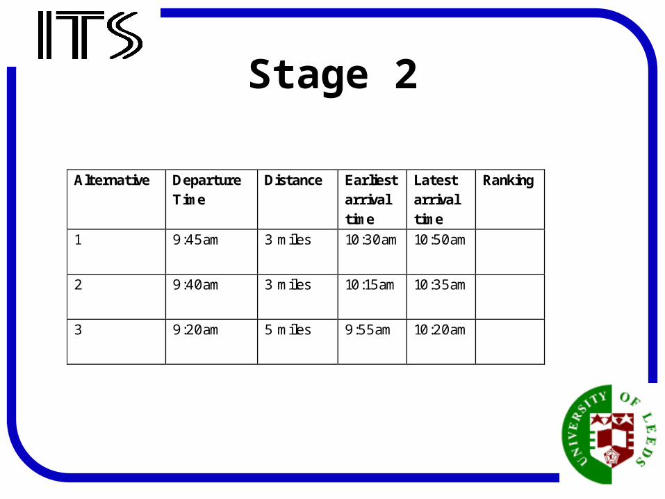
Stage 2

Alternative

Departure Time

Distance Earliest arrival time

Latest arrival time

Ranking

1 9:45am 3 miles 10:30am 10:50am

2 9:40am 3 miles 10:15am 10:35am

3 9:20am 5 miles 9:55am 10:20am

16

Field study• Members of staff at the York Health

Services Trust• Prize draw incentive• 165 usable first stage questionnaires• 56 usable second stage

questionnaires34% response rate for second stage

• Ranked data ‘exploded’ into binary choice data840 binary choice observations

17

MNL Parameter Estimate t-statistic βD 0.3202E-01 0.6 βG -0.1983E-01 -3.5 βQ 0.1472 8.9 βS 0.1265 7.3 Mean LL -0.595124 Observations 840

18

Random parameters logit

Utility to person n from alternative j at time t is specified:

njtnjtnnjtxU

where:

n ~ *f

njt ~ IID extreme value, independent of n and njtx

19

Random parameters logit

D e c o m p o s e :

nn b

w h e r e :

b i s m e a n , n i s s t o c h a s t i c d e v i a t i o n

njtnjtnnjtnjt xxbU

20

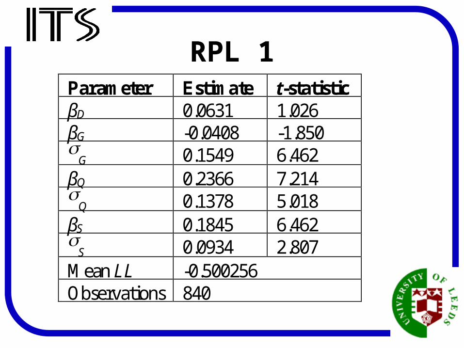
RPL 1 Parameter Estimate t-statistic βD 0.0631 1.026 βG -0.0408 -1.850

G 0.1549 6.462 βQ 0.2366 7.214

Q 0.1378 5.018 βS 0.1845 6.462

S 0.0934 2.807 Mean LL -0.500256 Observations 840

21

RPL 2 Parameter Estimate t-statistic βD 0.0680 1.214

cG -4.6982 -5.683 sG 2.2337 5.383

βG -0.1104

G 1.3335 cQ -1.6738 -11.005 sQ 0.6600 4.377

βQ 0.2332

Q 0.1723 cS -1.8661 -12.827 sS 0.3094 1.230

βS 0.1623

S 0.0514 Mean LL -0.537409 Observations 840

22

Summary• Where ‘panel’ data is available on

choices made by individuals, it is reasonable to assume that previous experiences somehow condition these choices

• Data set 1: RP route choice data– Random effects probit– Multi-period multinomial probit

• Data set 2: SP route and departure time choice– Pseudo-panel– Random parameters logit– Evidence of repeated observations effects