33

CHAPTER 2: SPATIAL DISTRIBUTIONS OF RECONSTRUCTED MASS AND MASS BUDGETS AND RECONSTRUCTED LIGHT EXTINCTION AND LIGHT-EXTINCTION BUDGETS

INTRODUCTION

The fine aerosol species at most IMPROVE sites can be classified into five major types: sulfates, nitrates, organics, light-absorbing carbon, and soil. However, at coastal locations such as the Virgin Islands and Brigantine, sea salt can be an important contributor to fine mass concentrations. The standard methods for apportionment of measured mass to the various aerosol species and the assumptions involved in those calculations are reviewed in section 2.1.

Atmospheric light extinction is a fundamental metric used to characterize air pollution impacts on visibility. It is the fractional loss of intensity in a light beam per unit of distance due to scattering and absorption by the gases and particles in the air. Light extinction (bext) can be expressed as the sum of light scattering by particles (bsp), scattering by gases (bsg), absorption by particles (bap), and absorption by gases (bag). The model used to reconstruct the light extinction coefficient from aerosol measurements and other visibility metrics for the sites are presented and examined below in section 2.2.

Spatial trends in reconstructed fine mass and the mass attributed to each of the major aerosol types are examined for the IMPROVE network and the IMPROVE and STN networks in section 2.4. The spatial trends in particulate extinction and the percent extinction attributed to each of the major aerosol types are examined in section 2.5 for the IMPROVE network and the IMPROVE and STN networks.

2.1 ESTIMATION OF AEROSOL SPECIES MASS

Table 2.1 presents the standard equations used in the IMPROVE program and those used in this report for estimating the aerosol species concentrations. The methodology behind those formulas and the limitations of the reconstructed fine mass (RCFM) aerosol model are discussed below.

The molecular form of sulfate depends on its degree of neutralization, for which routine measurements of the ammonium ion are required. The IMPROVE network does not measure the NH4

+ ion, and there are inherent sampling issues with respect to ammonium measurements [Hand and Malm, 2006]. The molar ratio of ammonium to sulfate ranges from 2 for fully neutralized ammonium sulfate to 0 for sulfuric acid. Many authors have shown that aerosol sulfate acidity can vary temporally and spatially. Acidic aerosols have been measured at many locations throughout the United States [Gebhart et al., 1994; Liu et al., 1996; Day et al., 1997; Lowenthal et al., 2000; Lefer and Talbot, 2001; Quinn et al., 2002; Chu, 2004; Hogrefe et al., 2004; Schwab et al., 2004; Tanner et al., 2004; Zhang et al., 2005]. Special studies at IMPROVE sites have also demonstrated variability. At Great Smoky Mountains National Park during the summer of 1995 (Southeastern Aerosol and Visibility Study, SEAVS), ammonium-to-sulfate molar ratios of 1.1 were observed [Hand et al., 2000]. During the Big Bend Regional Aerosol

34

and Visibility Observational (BRAVO) study at Big Bend National Park, Lee et al. [2004] found ammonium-to-sulfate molar ratios of 1.54 on average. On average, fully neutralized ammonium sulfate was measured at Yosemite National Park during the summer of 2002 [Malm et al., 2005]. Seasonal and spatial variations in aerosol acidity complicate the selection of a single form of ammoniated sulfate, and regular measurements of the NH4

+ ion at IMPROVE sites do not exist. Because the ammonium ion is not routinely measured in the IMPROVE program, sulfates will be assumed to be in the form of ammonium sulfate for the purpose of examining general spatial and temporal trends in sulfate aerosol mass concentrations.

Nitrate aerosols are assumed to be in the form of ammonium nitrate, but special studies have shown that at some locations fine nitrates are the fine tail of the coarse particle nitrate size distribution, such as sodium or calcium nitrate that has resulted from the reaction of nitric acid vapor with sea salt or soil dust [Malm et al., 2003; Lee et al., 2004; Hand and Malm, 2006]. The form of nitrate is difficult to predict since it depends on a number of factors including temperature, relative humidity, the presence of other aerosol species, and the cutpoint of the impactor [Hand and Malm, 2006]. Furthermore, Hand and Malm [2006], in a special study involving speciated and size-resolved aerosol samples from several IMPROVE sites, found that when fine mode total nitrate concentrations were roughly greater than 0.5 µg/m3, ammonium nitrate contributed over 70% of the observed total nitrate in the fine mode. Given that the measurements necessary to accurately determine the form of ammonium nitrate are unavailable and the indication that higher levels of nitrate in the fine mode are probably associated with NH4NO3, assuming that nitrate is in the form of ammonium nitrate is reasonable for reconstructing fine mass.

An average ambient particulate organic compound is assumed to have a constant fraction of carbon by weight. Historically in the IMPROVE program, organic carbon mass concentration (OMC) from module C was assumed to be [OMC] = 1.4[OC], where OC is organic carbon as determined by thermal optical reflectance (TOR). The value of 1.4 was based on an experiment conducted by Grosjean and Friedlander [1975] in urban Pasadena, California, in 1973. They found that the carbon content of these samples averaged 73%. White and Roberts [1977] suggested an OC to OMC conversion factor (OMC/OC) of 1.4 based on this data, and this value was incorporated into the IMPROVE reconstructed fine mass equation. More recently, the ratio of OMC to OC used by IMPROVE has been changed to a value of 1.8, based on the suggestion of Hand and Malm [2006] and the studies summarized therein indicating that a correction factor of 1.4 is probably unreasonably low for the IMPROVE network and that 1.8 is a reasonable consensus value based on the available data.

Soil taxonomy charts show variability across the United States with soil type, with the southwestern United States differing from the eastern United States and many finer differentiations beyond that. Soil composition can also vary due to long-range intercontinental and transcontinental transport. Several studies have shown that contributions of Asian dust to U.S. fine soil aerosol concentrations can be significant episodically, affecting aerosol concentrations and mineralogy across the United States in the spring [VanCuren and Cahill, 2002; Jaffe et al., 2003; VanCuren, 2003; DeBell et al., 2004]. In the late spring to midsummer, transport of North African dust to the United States occurs regularly, affecting aerosol concentrations in the Virgin Islands, the eastern United States [Perry et al., 1997; Prospero, 1999], and even as far west as Big Bend National Park [Hand et al., 2002]. Due to the spatial

35

and temporal variability in dust sources, it is very difficult to characterize an appropriate aerosol soil composition for each measurement site. Soil mass concentrations are therefore estimated by a general method that sums the oxides of elements that are typically associated with soil (Al2O3, SiO2, CaO, K2O, FeO, Fe2O3, TiO2), with a correction for other compounds such as MgO, Na2O, H2O, and carbonates [Malm et al., 1994]. The soil K is estimated from the Fe and Fe/K ratios because of the nonsoil K contributions from other sources, including smoke. Elemental concentrations are multiplied by factors that represent the mass concentrations of the oxide forms, with several corrections made to account for the previously mentioned compounds.

Coarse mass concentrations (CM) are estimated by differencing the PM10 mass measurement and the PM2.5 measurement. Deviations from the nominal flow rate due to filter clogging from high aerosol loading and other operational problems can cause the cutpoint of the PM2.5 A module to vary and affect which modes of the size distribution are being classified as fine and coarse.

Because Teflon filters are prone to losses of semivolatile NH4NO3 and thus provide only a lower estimate of the actual ambient aerosol concentrations, comparisons of reconstructed fine mass using the IMPROVE equation and gravimetric fine mass can be highly affected. Other factors such as retained water on the Teflon filter can also impact reconstructed fine mass to gravimetric fine mass comparisons.

Table 2.1. IMPROVE equations.

Aerosol Type Traditional IMPROVE Equation Revised Equation

Assumptions

Ammonium Sulfate

4.125*[S] Same All elemental S is from sulfate. All sulfate is in the form of ammonium sulfate.

Ammonium Nitrate

1.29*[NO3] Same Denuder efficiency is close to 100% for HNO3. All nitrate is in the form of ammonium nitrate.

Organic Mass by Carbon (OMC)

1.4*[OC] 1.8*[OC] Average organic molecule is 55% (70% for the 1.4 correction factor) carbon.

Light-Absorbing Carbon (LAC)

[LAC] Same

STN Light-absorbing Carbon (LAC_STN)

NA [LAC_STN]

Adjusted STN Organic Carbon (OC_STN)

NA [OC_STN]-[blank correction]

Organic carbon from STN NIOSH adjusted for method specific blank correction.

Total Carbon NA [OC]+[LAC] or [OC_STN]+[LAC_STN]

No organic carbon correction.

36

Aerosol Type Traditional IMPROVE Equation Revised Equation

Assumptions

Soil 2.2*[Al]+2.49*[Si]+1.63*[Ca]+ 2.42*[Fe]+1.94*[Ti]

same Soil potassium=0.6*[Fe] FeO and Fe2O3 are equally abundant. A factor of 1.16 is used for MgO, Na2O,H2O, CO3.

Reconstructed Fine Mass

[Ammonium Sulfate]+ [Ammonium Nitrate]+[LAC]+[OMC]+ [Soil]

same Represents dry ambient fine aerosol mass. Comparability of OC and OC_STN.

Coarse Mass [PM10]-[PM2.5] Same A PM2.5 cut point on the fine mass sample. A PM10 cut point on the coarse mass sample.

2.2 RECONSTRUCTING LIGHT EXTINCTION FROM AEROSOL MEASUREMENTS

The light-extinction coefficient, bext (expressed as inverse megameters, Mm-1), is the sum

where bscat is the sum of scattering by gases and scattering by particles, and babs is the sum of absorption by gases and particles. Light extinction due to the gaseous components of the atmosphere are relatively well understood and well estimated for any atmospheric condition. Absorption of visible light by gases in the atmosphere is primarily by NO2 and can be directly and accurately estimated from NO2 concentrations by multiplying by the absorption efficiency. Scattering by gases, bsg, is described by the Rayleigh scattering theory [van de Hulst, 1981]. Rayleigh scattering depends on the density of the atmosphere; the highest values are at sea level (about 12 Mm-1) and they diminish with elevation (8 Mm-1 at about 12,000′) and vary somewhat at any elevation due to atmospheric temperature and pressure variations. Rayleigh scattering can be accurately determined for any elevation and meteorological condition.

Particle light extinction is more complex than that caused by gaseous components. Light-absorbing carbon (e.g., diesel exhaust soot and smoke) and some crustal minerals are the only commonly occurring airborne particle components that absorb light. All particles scatter light, and, generally, particle light scattering is the largest of the four light extinction components. If the index of refraction as a function of particle size is well characterized, Mie theory can be used to accurately calculate the light scattering and absorption by those particles. However, it is rare that these particle properties are known, so assumptions are used in place of missing information to develop a simplified calculation scheme that provides an estimate of the particle light extinction from the available data set.

b+b+b+bbb=b apagspsgabsscatext =+ (2.1)

37

2.2.1 Extinction Model

The traditional IMPROVE algorithm for estimating light extinction from IMPROVE particle monitoring data assumes that absorption by gases (bag) is 0, that Rayleigh scattering (bsg) is 10 Mm-1 for each monitoring site regardless of site elevation and meteorological condition, and that particle scattering and absorption (bsp and bap) can be estimated by multiplying the concentrations of each of six major components by typical component-specific light extinction efficiencies. The component extinction efficiency values are constants, except for the sulfate and nitrate extinction efficiency terms that include a water growth factor that is a function of relative humidity (displayed as f(RH)), multiplied by a constant dry extinction efficiency. Expressed as an equation, the algorithm used in this report for estimating light extinction from IMPROVE data takes the following form where the particle component concentrations are indicated in the brackets. The formulas for the composite components are given in section 2.1.

[ ][ ]

[ ][ ]

[ ][ ]

106.0

1104

)(3)(3

+×+

×+×+×+

××+××≈

MassCoarseSoilFine

CarbonElementalMassOrganic

itrateAmmonium NRHfulfateAmmonium SRHfbext

(2.2)

The units for light extinction and Rayleigh scattering are inverse megameters (Mm-1); component concentrations shown in brackets are in microgram per meter cubed (µg/m3); dry efficiency terms are in units of meters squared per gram (m2/g); and the water growth terms, f(RH), are unitless.

Among the implicit assumptions for this formulation of the algorithm are that

• the six particle component terms plus a constant Rayleigh scattering term are sufficient for a good estimate of light extinction;

• constant dry extinction efficiency terms rounded to one significant digit for each of the six particle components (e.g., for both sulfate and nitrate the value is 3) works adequately for all locations and times; and

• light extinction contributed by the individual particle components can be adequately estimated as separate terms, as they would be if they were in completely separate particles (externally mixed), though they often are known to be internally mixed in particles.

A relatively simple algorithm for estimating light extinction using only the available monitoring data requires assumptions such as these.

The issue of estimating aerosol optical properties from bulk aerosol measurements that do not allow for determining the mixing state of the aerosol has been addressed. Ouimette and

38

Flagan [1982] have shown that, from basic theoretical considerations, if an aerosol is mixed externally, or if in an internally mixed aerosol the index of refraction is not a function of composition or size, and the aerosol density is independent of volume, then

∑α=i

iiext mb (2.3)

where αi is the specific scattering or absorption efficiency and mi is the mass of the individual species.

Furthermore, Malm and Kreidenweis [1997] demonstrated from a theoretical perspective that specific scattering of mixtures of organics and sulfates were insensitive to the choice of internal or external mixtures. Sloane [1983, 1984, 1986], Sloane and Wolff [1985], and more recently, Lowenthal et al. [1995], Malm et al. [1997], and Malm [1998] have shown that differences in estimated specific scattering between external and internal model assumptions are usually less than about 10%. In the absence of a detailed microphysical and chemical structure of ambient aerosols, the above studies demonstrate that a reasonable estimate of aerosol extinction can be achieved by assuming each species is externally mixed.

Implicit to the extinction model is an assumed linear relationship between aerosol mass and extinction. It is well known that sulfates and other hygroscopic species form solution droplets that increase in size as a function of relative humidity (RH). Therefore, if scattering is measured at various relative humidities, the relationship between measured scattering and hygroscopic species mass can be quite nonlinear. The approach of Gebhart and Malm [1989] and Malm et al. [1989] for estimating the effect of RH on aerosol scattering is the basis for the method employed in the IMPROVE extinction model. In their approach, the hygroscopic species are multiplied by a relative humidity scattering enhancement factor, f(RH), that is calculated on a sampling-period-by-sampling-period basis using Mie theory and an assumed size distribution and laboratory-measured aerosol growth curve. However, because the growth factor and light-scattering efficiency for ambient aerosols have previously been observed to be rather smooth [Waggoner et al., 1981; Sloane 1983, 1984, 1986; Wexler and Seinfeld, 1991; Day et al., 2000; Malm et al., 2000a], the laboratory growth curves, as measured by Tang [1996], were smoothed between the deliquescence and crystallization points to obtain a “best estimate" for the sulfate and nitrate species growth (Figure 2.1).

39

Figure 2.1. RH factors (fT (RH)) derived from Tang’s ammonium sulfate growth curves smoothed between the crystallization and deliquescence points.

For the data used in this report, the f(RH) values for each sample are calculated using the algorithm outlined in the Regional Haze Rule Guidelines for Tracking Progress [U.S. EPA, 2003]. Under this algorithm, fSO4(RH) values for each sampling period are calculated by assuming a typical site-specific RH value, a lognormal sulfate mass size distribution with a geometric mass mean diameter of 0.3 µm and a geometric standard deviation, σg, of 2.0, and growth curves that are smoothed between the crystallization and deliquescence points. The fNO3(RH) associated with nitrates is assumed to be the same as for sulfates, while forg(RH) for organics is set equal to 1.0.

Month-specific climatological mean RH values were chosen to eliminate the confounding effects of interannual variations in relative humidity while maintaining typical regional and seasonal humidity patterns. The EPA produced a lookup table with recommended monthly f(RH) values for each Class I area based on analysis of a 10-year record (1988–1997) of hourly relative humidity data from 292 National Weather Service stations across the 50 states and the District of Columbia, as well as from 29 IMPROVE and IMPROVE protocol monitoring sites, 48 Clean Air Status and Trends Network (CASTNet) sites, and 13 additional sites administered by the National Park Service. The daily ammonium sulfate and ammonium nitrate extinction coefficients for each site are calculated using this lookup table.

In a recent review, estimates of particle scattering by the IMPROVE algorithm (i.e., excluding the light-absorbing carbon and Rayleigh terms) were compared to directly measured particle scattering data at the 21 monitoring sites that have hourly averaged nephelometer and relative humidity data [IMPROVE technical subcommittee for algorithm review, 2006]. The results indicated that the algorithm performed reasonably well over a broad range of particle light scattering values and monitoring locations. However, the algorithm does tend to underestimate

40

the highest extinction values and overestimate the lowest extinction values. A revised algorithm that reduces these biases has recently been approved by the IMPROVE steering committee as an alternative method for calculating reconstructed extinction. The new algorithm with revised terms in bold has the following form:

( ) [ ] [ ]( ) [ ] [ ]

[ ] [ ][ ]

[ ]( ) [ ]

[ ]

[ ](ppb) NO0.33Specific) (Site Scattering Rayleigh

MassCoarse0.6SaltSea RHf1.7

Soil Fine1Carbon Elemental10

MassOrganic Large6.1 MassOrganic Small2.8Nitrate Large(RH)f5.1Nitrate SmallRHf2.4

Sulfate Large(RH)f4.8Sulfate SmallRHf2.2b

2

ss

Ls

Ls

ext

×++

×+

××+×+×+

×+×+

××+××+

××+××≈

(2.4)

The apportionment of the total concentration of sulfate compounds into the

concentrations of the small and large size fractions is accomplished using the following equations:

[ ] [ ] [ ] [ ] 33 /mg µ 20SulfateTotalfor,SulfateTotal

µg/m 20SulfateTotalSulfateeargL <×=

[ ] [ ] [ ] 3µg/m 20Sulfate Totalfor ,Sulfate TotalSulfate Large ≥= [ ] [ ] [ ]SulfateeargLSulfateTotalSulfateSmall −=

The same equations are used to apportion total nitrate and total organic mass concentrations into the small and large size fractions. The algorithm used for calculating the new terms and the technical justification of the changes are detailed here: http://vista.cira.colostate.edu/improve/Publications/GrayLit/019_RevisedIMPROVEeq/RevisedIMPROVEAlgorithm3.doc.

Comparisons of the revised and original IMPROVE extinction algorithms indicated that the composition associated with the average best and worst haze days was fairly insensitive to algorithm selection [IMPROVE technical subcommittee for algorithm review, 2006]. Therefore only results utilizing the original algorithm, modified to include the new organic mass to organic carbon ratio, are shown here. Speciated extinction values calculated using the new and original algorithm are available from the IMPROVE website at http://vista.cira.colostate.edu/views/Web/Data/DataWizard.aspx. Interested readers can explore both data sets by either downloading the data for themselves or utilizing the data exploration tools provided by the VIEWS website at http://vista.cira.colostate.edu/views/Web/General/AnnualSummary.aspx.

41

Visibility, expressed as the reconstructed deciview (dv), is calculated from the reconstructed total extinction values. The dv is a visibility metric based on the light extinction coefficient that expresses incremental changes in perceived visibility [Pitchford and Malm, 1994]. Because the dv expresses a relationship between changes in light extinction and perceived visibility, it can be useful in describing visibility trends. A 1-dv change is about a 10% change in extinction coefficient, which is a small but perceptible scenic change under many circumstances. The dv is defined by the following equation:

)/ln( 10b10dv ext= (2.5)

The dv scale is near 0 for pristine atmosphere (dv = 0 for Rayleigh condition at about 1.8 km elevation) and increases as visibility is degraded.

2.3 COMPLETENESS CRITERIA

For the following analyses, data from a particular site are only included if they meet certain completeness criteria. The completeness criteria used in Chapters 2 and 3 of the report are designed to ensure that as many sites as possible are included in the analyses without jeopardizing the robustness or representativeness of the results. These criteria are not the same criteria as applied under Regional Haze Rule guidelines, which have different objectives than this report. The goal of these analyses was to look at general trends in the central tendency of the aerosol parameters, rather than analyzing the individual days that make up the worst and best haze days.

Since results are supposed to be representative of the 5-year period 2000–2004, it was decided that the equivalent of two-fifths of the potential samples, or ~2 years’ worth, needed to be valid for the site to be considered complete. Furthermore, similar criteria are applied to each of the four seasons, ensuring that the annual averages are not overly biased by exclusion of samples from a particular season. A site was required to have its first valid sample on or before 1 February 2003 to be included in the following analyses, figures, and tables. Additionally, it was required that each seasonal bin have at least 50 valid samples. Seasonal distribution of the valid samples beyond the minimum per bin was not examined. These criteria are applied at the parameter level, not the record level, e.g., completeness is assessed for organic carbon independently of sulfate or any other parameter of interest. These requirements are a slight departure from similar analyses reported in prior IMPROVE reports where filtering only took into account the start date of the site in question.

In keeping with the parameter-level application of completeness criteria, the sorting and aggregation of data by time and space are also conducted at the parameter level. This process and its implications are detailed in Malm et al. [2000b] and will be described here briefly. As an example, the calculation of the average RCFM for Acadia for the 2000–2004 period will be used to illustrate this topic. Two approaches can be taken in calculating this “average”, the sum of the averages or the average of the sums:

1) Avg(RCFM)=Avg(NO3)+ Avg(SO4)+ Avg(OMC)+ Avg(LAC)+ Avg(SOIL)

2) Avg(RCFM)= Avg(NO3+SO4+OMC+LAC+SOIL)

42

The second approach, the average of the sums, requires that each sample day be complete, with valid measurements for all five major parameters for inclusion in the 5-year average. The problems with using the stricter completeness criteria dictated by approach 2 include unacceptably small sample sizes in some data aggregates and the exclusion of some records where very high or low aerosol concentrations have resulted in invalid values for a subset of the parameters. The analyses in this report make use of the first equation since it includes all valid samples for a parameter regardless of the sampling completeness for an individual date, and in that sense the data aggregates more accurately represent the average atmospheric conditions.

2.4 SPATIAL TRENDS IN AEROSOL CONCENTRATIONS IN THE UNITED STATES

Estimated spatial trends of annual average species concentrations across the United States were presented by Malm et al. [1994] for the 3-year period of March 1988 through February 1991 using data collected at 36 monitoring sites. Of the 36 monitoring sites, only 4 (including Washington, D.C.) were located in the eastern United States, and therefore any east/west or north/south trends east of a line from North Dakota to Texas were speculative at best. The spatial variability of the 2001 annual average aerosol species concentrations were reported in Malm et al. [2004] using data collected at 143 sites, 49 of which were eastern United States monitoring sites, allowing for a significantly better understanding of spatial and short-term temporal (monthly) trends in that region of the country.

Here, the spatial variability of the annual average aerosol species concentrations for the 5-year period January 2000 through December 2004 is explored. The annual average aerosol components are presented in Figures 2.2–2.9 as isopleth maps. Data collected at 157 IMPROVE monitoring sites and 69 STN monitoring sites met the completeness criteria for all five RCFM components; an additional 2 IMPROVE sites and 15 STN sites met completeness criteria for a subset of the RCFM components. All sites that met completeness criteria for a given RCFM component were included in the analysis and are depicted on the maps. The isopleth values between the monitoring sites are not meant to represent the concentrations in these areas; instead, they are meant to help identify large spatial patterns in the monitored data. Spatial patterns in both aerosol concentration and percent contribution to reconstructed fine mass are explored for each aerosol component. Additionally, the change in spatial patterns that results from the addition of urban sites from the STN is also examined. IMPROVE sites are indicated on the maps with circles and STN sites are indicated with triangles.

2.4.1 Fine Particle Ammonium Sulfate Mass

Figure 2.2, panels a and c, show isopleths maps of fine particulate sulfur interpreted as ammonium sulfate and the fractions of reconstructed fine mass that are attributed to ammonium sulfate, expressed as a percentage of RCFM for the IMPROVE network. Panels b and d show the same results for the IMPROVE and STN networks. Sulfates are primarily a product of sulfur dioxide (SO2) emissions and photochemical reactions in the atmosphere. For example, sulfates tend to be highest in areas of significant SO2 emissions such as the eastern United States where SO2 is emitted from coal-fired stationary sources [Malm et al., 1994, 2002]. The highest annual average rural ammonium sulfate mass concentrations were found in the central eastern United

43

States, where concentrations at most sites were in the 4.5–6.5 µg/m3 range (Appendix A). The addition of the STN sites stretches the Ohio River valley high concentration region, where concentrations were greater than 5.25 µg/m3, in all directions. From the high concentration region, ammonium sulfate concentrations decrease to the northeast, southeast, and west. The higher sulfate concentration isopleths were extended farther west by the addition of the east Texas and Gulf Coast STN sites, as compared to the rural spatial trends identified in the analysis of IMPROVE. The east-to-west gradient is particularly striking, with concentrations in the central eastern United States a factor of 8 higher than the western sites. Both the rural noncontiguous United States sites in Hawaii and the Virgin Islands and the urban site in Puerto Rico had concentrations between 1 and 2.25 µg/m3. The rural and urban sites in Alaska had ammonium sulfate concentrations in the 0.5–1 µg/m3 range.

In general, the east-to-west gradient is so much stronger than the urban-to-rural gradients that the latter are difficult to identify in the isopleth maps. Urban ammonium sulfate concentrations generally did not exceed 2 times nearby rural concentrations. The exceptions to this were the urban sites, STN and IMPROVE, in the northwestern states of Oregon, Washington, Colorado, Utah, and Idaho, which had ammonium sulfate concentrations at least 2 times higher than nearby rural concentrations. Given the mountainous locations of many of the IMPROVE sites in these states, the impact of elevation on the urban-rural contrast must be considered. The rural sites in Colorado and Idaho were all between 600 and 2000 m above Denver and the Wasatch Front STN sites, correspondingly. There were significant elevation gradients (>1000 m) between the urban and rural sites in Oregon, Washington, and Utah as well, but there were also rural sites at similar elevations to the urban sites (within 50 m) that still showed urban concentrations of at least 2 times rural concentrations. Elevation gradients likely contribute to at least a portion of the sites in these states exhibiting high urban-rural contrast in ammonium sulfate. Because of the relatively low contrast between urban and nearby rural sites, the general spatial trends observed in rural concentrations were not greatly modified by the addition of urban sites to the analysis. However, there were noticeable changes such as the extension of the high concentration region in the central eastern United States. Of the five RCFM components, spatial trends in ammonium sulfate were the least affected by the addition of urban sites to the analysis.

Referring to Figures 2.2c and 2.2d and Appendix A, which lists the annual average concentrations for 2000–2004, there were 25 sites in the eastern United States and Hawaii where ammonium sulfates make up over 50% of RCFM. The fractional contribution of ammonium sulfate to RCFM generally decreases to the west and to the east along the Atlantic coast. Much of the northwestern United States had less than a 20% ammonium sulfate contribution to RCFM. Fractional contributions increase again along the Pacific coast, particularly at the coastal sites in California—Agua Tibia, Point Reyes National Seashore, Redwoods National Park, and San Rafael—where the percent contributions were all 30% or greater, which makes them more similar to sites east of the Continental Divide than the other western sites. The general patterns observed here in the 2000–2004 period for the combined IMPROVE and STN data set are consistent with those observed by Malm et al. [2004] for the 2001 IMPROVE data and are not significantly altered by the addition of the 82 urban STN sites.

44

2.4.2 Fine Particle Carbon Mass

Organic aerosols have their origin in both primary emissions and from secondary aerosol formation. For instance, primary organic carbon emissions have been linked to meat cooking, road dust, mobile sources, fire-related activity, and industrial activities in the Los Angeles Basin [Rogge et al., 1996] and, more generally, to fire-related activity in all parts of the United States [Hawthorne et al.,1992; Schmidt et al., 2002], while secondary organic aerosols are formed from gaseous precursors that have both biogenic [Hatakeyama et al., 1989; Izumi and Fukuyama, 1990; Kavouras et al., 1998a, 1998b; Jang and Kamens, 1999] and anthropogenic [Izumi and Fukuyama, 1990; Odum et al., 1996, 1997; Holes et al., 1997; Jang and Kamens, 2001] origins. Light-absorbing carbon particles are produced from the combustion of carbon-based fuels, with the major sources including diesel engines, biomass burning, and coal combustion [Bond and Bergstrom, 2005].

The side-by-side analysis of urban and rural carbon measurements is complicated by different measurement techniques for IMPROVE and the STN and by the differences in the average carbon multiplier for urban and rural areas. The separation point between OC and light-absorbing carbon (LAC) is procedurally defined, and thus the reported OC and LAC fractions from the IMPROVE and STN networks are not expected to be equal. Another major distinction between the IMPROVE and STN carbon measurements is the lack of blank correction for the reported STN measurements. However, the STN OC measurements reported here are blank corrected as described in Appendix E. Given that the OC and LAC are not expected to be equal, it was surprising that collocated IMPROVE and STN data showed the blank-corrected OC measurements from the STN to be quite comparable with less than a 1% difference between annual averages in the organic carbon concentrations. However, the STN LAC average concentrations were ~10% lower than from the collocated IMPROVE samplers. Furthermore, urban and rural aerosols have been shown to be best modeled with different carbon multipliers, with lower values recommended for urban aerosols [Turpin and Lim, 2001]. Therefore spatial trends in LAC and OC between STN and IMPROVE sites should be considered to have greater uncertainty than spatial trends observed in ammonium sulfate and nitrate. Since total carbon (TC) measurements are expected to be equivalent and are also free of the complication of an assumed organic carbon multiplier, spatial trends in TC are examined even though TC is not a component of the RCFM model.

The rural IMPROVE TC mass concentrations for the contiguous United States ranged from 0.6 to 3.0 µg/m3, with ~80% of the sites having concentrations less than 2 µg/m3 (Figure 2.3a). The noncontiguous U.S. sites—Alaskan, Virgin Island, and Hawaiian—all had TC concentrations less than 0.5 µg/m3. The highest rural TC concentrations, greater than 2.5 µg/m3, were found at the same sites, with peak OMC concentrations in the southeastern United States and the Sierra Nevada region (Appendix A). Intermediate TC concentrations of 1.5–2.25 µg/m3 are found throughout much of the eastern and northwestern (including northern California) United States and in the Sierra Nevada and southern California regions. The TC concentrations at the STN urban sites ranged from 0.9 µg/m3 in upstate New York to 7.8 µg/m3 in the San Joaquin Valley of California, with ~60% of the sites having concentrations between 2 and 4 µg/m3 (Figure 2.3b). All of the western states with urban and rural sites available for comparison (Alaska, California, Oregon, Washington, Montana, Idaho, Nevada, Utah, Arizona, Texas, Kansas, and Nebraska) had urban TC concentrations at least 2 times higher than nearby rural

45

concentrations. In the East, this high degree of contrast between urban and rural concentrations was only present in Alabama, North Carolina, Ohio, and New Hampshire.

Organic mass by carbon concentrations and fractional contributions to RCFM are shown in Figure 2.4a–d. OMC concentrations were above 1 µg/m3 at nearly all IMPROVE sites. Of the eight sites with organic mass concentrations below 1 µg/m3, five are sites located outside of the contiguous United States (Simeonof and Tuxedni, Alaska; Hawaii Volcanoes National Park and Haleakala, Hawaii; and the Virgin Islands) and two are among the highest elevation sites in this analysis (Wheeler Peak, New Mexico, and White River, Colorado); the eighth site, White Pass, Washington, is the highest elevation site in the Northwest region. Peak rural values of 4–5 µg/m3 occurred at the Spokane reservation in the Northwest, Sequoia National Park in the Sierra Nevada region, Mingo in the mid-South region, and at several sites in the southeastern United States. A large band through the interior West from the Mexico border into the upper Midwest had rural OMC concentrations less than 2 µg/m3 at most sites. Most of the rural eastern and northwestern United States, along with northern and southern California and the Sierra Nevada mountains, had OMC concentrations in the 2–4 µg/m3 range.

Using the same adjustment factor for calculating urban and rural OMC concentrations, the OMC concentrations at the three urban IMPROVE sites were between 4.5 and 6 µg/m3. Phoenix and Puget Sound concentrations were 2–5 times higher than the nearby rural sites, indicating large local sources. Compared to the analysis of ammonium sulfate, the addition of the urban STN sites more extensively altered the spatial trends in peak OMC mass concentrations. Localized high concentration areas outside of the southeastern United States and California were identified with the inclusion of the urban sites. The STN urban sites had OMC concentrations ranging from 1.3 µg/m3 in upstate New York to 12.4 µg/m3 in the San Joaquin Valley of California with ~60% of the sites having concentrations between 2 and 6 µg/m3. All of the western states with urban and rural sites available for comparison (Alaska, California, Oregon, Washington, Montana, Idaho, Nevada, Utah, Arizona, Texas, Kansas, and Nebraska) had urban concentrations at least 2 times higher than nearby rural concentrations. In the East, this high degree of contrast between urban and rural concentrations was only present in Alabama, Kansas, North Carolina, and New Hampshire; the other eastern states where a comparison was possible had urban concentrations that did not exceed 2 times nearby rural concentrations.

There was greater dissimilarity between the spatial trends in the fractional contribution of OMC to RCFM and the trends in OMC concentrations than was the case for ammonium sulfate. The highest OMC contributions to RCFM all occurred in Alaska and the northwestern United States where they were nearly all above 40% and exceeded 60% at approximately half of these sites. In rural southern California, the Colorado and Mogollon plateaus, the northern Great Plains, the Rockies, the Boundary Waters, New England, and the southeastern United States, percent contributions of OMC were typically in the 30–50% range. Organics only contributed in the range of 20–30% to RCFM in the remainder of the rural contiguous United States, principally from the Central Great Plains through the Ohio River valley and northern Appalachia range into upstate New York, with additional pockets in the arid Southwest and along the coasts. Puerto Rico and Hawaii also had OMC contributions in the 20–30% range. The Virgin Islands was the only location to have organics contribute less than 20% to RCFM. The most obvious effects of adding the urban STN sites to the analysis are the extension of the high contributions regions in

46

the Northwest, south to central California, and east to eastern Montana and adding hot spots to the high contribution region in the southeastern United States.

Rural light-absorbing carbon mass concentrations, with a few exceptions, were below 0.5 µg/m3; the four exceptions, Old Town, Maine; M.K. Goddard, Pennsylvania; Mingo, Missouri; and James River Face Wilderness, Virginia, all had concentrations very near to 0.5 µg/m3 (Figure 2.5a). The highest average LAC concentrations, those greater than 0.4 µg/m3, occurred in the eastern United States and California, with over half of these sites concentrated in the Ohio River valley and Appalachian region. The high LAC concentration region in the East roughly corresponds to the high ammonium sulfate region. Similar to OMC, there is a large low concentration band through the interior West, where LAC concentrations were generally less than 0.2 µg/m3. Much of the rural eastern and northwestern United States, along with the Sierra Nevada and southern California regions, had LAC concentrations in the 0.2–0.4 µg/m3 range. Urban LAC concentrations ranged from 0.2 in upstate New York to 2.3 µg/m3 in Puerto Rico, with ~70% of the sites having concentrations between 0.3 and 1 µg/m3. Light-absorbing carbon contributes less than 10% to RCFM at all rural sites, with the highest fractional contributions occurring at Glacier National Park, Montana; Old Town, Maine; and Snoqualmie Pass and Mount Rainier National Park, Washington (Figure 2.5b). Urban LAC contributions were less than 10%, with the exceptions of Alaska, southeastern Florida, and Puerto Rico where contributions were 10%, 15%, and 26%, respectively.

2.4.3 Fine Particle Ammonium Nitrate Mass

The annually averaged nitrate concentrations and the nitrate fractions of RCFM are shown in Figure 2.6a–d. The fine particulate nitrate mass concentrations were interpreted as ammonium nitrate. Since nitrate concentrations are dependent on a number of factors, including nitrogen oxide and ammonia emissions, photochemical reactions, temperature, humidity, and the presence of other aerosol species, many factors contribute to where high aerosol nitrate concentrations are formed. Rural ammonium nitrate concentrations were highest at the central and southern California sites and in the Midwest, where both nitrogen oxide and ammonia emissions are high [U.S. EPA, 2000]. Urban IMPROVE and STN sites indicate additional high concentration areas in the Sacramento Valley of California, Idaho, Utah, Colorado, Texas, New York, and Pennsylvania. The highest concentrations occur at the urban sites in southern California, peaking at 14 µg/m3 in Los Angeles. The Central Great Plains region is the largest area of high ammonium nitrate concentrations, with rural concentrations typically between 2 and 3 µg/m3 and the urban concentrations between 3 and 4 µg/m3. From the high concentration region in the Midwest, rural ammonium nitrate concentrations generally decrease to the east, south, and west until higher concentrations are again encountered along the Pacific coast. The extreme Northeast and the interior West have concentrations that are typically less than 0.5 µg/m3.

Similar to TC, the western states of Alaska, California, Oregon, Washington, Montana, Idaho, Nevada, Utah, and Arizona all had urban concentrations at least 2 times higher than nearby rural concentrations. In the East, urban ammonium nitrate concentrations less commonly exceeded 2 times nearby rural concentrations. The exceptions in the East, where a high degree of urban-rural contrast existed, were North Carolina, Ohio, Tennessee, Massachusetts, New Hampshire, and Vermont. Additionally, the states that had the largest absolute differences

47

between the highest urban concentrations and surrounding rural sites, 2–4 µg/m3, were Colorado, Utah, Idaho, New York, Michigan, and Ohio. Central and southern California had urban excess ammonium nitrate concentrations in the 2–12 µg/m3 range, but northern California and Oregon were in the 0.75–1.25 µg/m3 range. The comparison of the northern Minnesota rural sites to urban sites results in urban excess values of ~2 µg/m3, but the southern Minnesota rural sites were within 0.5 µg/m3 of the highest urban concentrations.

The spatial trends in the fractional contribution of nitrates to RCFM reflect the spatial trends in nitrate concentration. The highest percent contributions of 25–45% occur in the Midwest, central and southern California, and urban Idaho and Utah. The areas surrounding the highest contribution regions—parts of the Midwest, northern California, the Northeast, the Northwest, and southern Arizona—all have contributions in the 10–20% range. Nitrate contributions were generally less than 10% in New England, the Southeast, the interior West, and much of the northwestern United States.

2.4.4 Fine Particle Soil Mass

Figure 2.7a–d shows the annual average spatial distribution for the 2000–2004 period of fine soil mass concentrations and the soil fractions of RCFM. The highest rural fine soil concentrations were found in the arid Southwest at Sycamore Canyon and the west and east units of Saguaro National Park, Arizona, at 2.61, 3.08, and 2.18 µg/m3, respectively. The Virgin Islands, the Queen Valley in southern Arizona, and the west Texas sites of Guadalupe Mountain and Salt Creek all had concentrations in the 1.5–2 µg/m3 range. Rural soil mass concentrations in the range of 1–1.5 µg/m3 were found in southern Colorado; the Death Valley National Monument, California; El Dorado Springs, Missouri; in the Cherokee Nation, Oklahoma; and throughout most of Arizona. For most of the rural United States, soil mass concentrations were between 0.5 and 1 µg/m3, with the Great Lakes area, the northern Rockies, Alaska, Hawaii, and the northwestern and northeastern United States generally having soil concentrations less than 0.5 µg/m3. The spatial patterns in fine soil were quite distinct from those for ammonium sulfate, ammonium nitrate, and organic mass by carbon—it is the only fine aerosol parameter to show peak concentrations in the arid Southwest.

The peak soil concentration of 4.8 µg/m3 occurs at an urban STN site in El Paso, Texas. The annual average soil concentration at this site in El Paso is 2–3 times the other STN El Paso site and the IMPROVE sites in western Texas. The next highest urban site, the IMPROVE Phoenix, Arizona, site, had at 2.93 µg/m3 a comparable concentration to the peak rural concentrations in Arizona. The STN Puerto Rico site and the IMPROVE Spokane site also have soil concentrations greater than 2 µg/m3. The Spokane reservation site had annual soil concentrations that were between 2 and 10 times the other urban and rural sites in Washington and northwestern Montana. Urban soil mass concentrations in the range of 1–2 µg/m3 were found in Arizona and west Texas, as well as in Alabama, California, Colorado, Florida, Missouri, Nebraska, and Ohio. For most of the United States, urban soil mass concentrations were in the same concentration range as at nearby rural sites. The exceptions include Alaska, Alabama, Nebraska, and Ohio where the urban concentrations were over 2 times those at the rural sites in the state. Soil concentrations in Denver were twice those at the northern Colorado sites and the Weminuche Wilderness and similar to the Great Sand Dunes and Mesa Verde national parks.

48

The additions of the STN Missoula site and the southwestern Pennsylvania site extend the 0.5–1 µg/m3 isopleth west and north, respectively.

As was the case with ammonium nitrate, the spatial trends in fractional contribution of soil to RCFM reflect the spatial trends in soil concentration. The highest fractional contribution from soil occurs in the Virgin Islands at 51%. The Virgin Islands and Barbados have both been shown to have significant dust aerosol inputs from the African deserts [Perry et al., 1997; Prospero, 1999]. From there the highest fractional contributions were associated with the highest soil concentrations; Sycamore Canyon and the west and east units of Saguaro National Park had soil contributions in the range of 35–45%. Soil contributions ranged from 30% to 35% at Chiricahua National Monument, Queen Valley, and Hillside, Arizona; Great Sand Dunes National Monument, Colorado; Death Valley National Park, California; and Guadalupe Mountains National Park, Texas. Most of the remaining rural southwestern sites, including the IMPROVE Phoenix site, had soil contributions in the 20–30% range. Puerto Rico was the only STN site to have soil contributions greater than 20% (Appendix A). Outside of the southwestern United States, the rural interior West and the Everglades National Park, Florida, had soil contributions in the 10–20% range. Florida also has regular inputs of dust aerosol from Africa [Perry et al., 1997; Prospero, 1999]. STN sites in western Texas; Phoenix, Arizona; Denver, Colorado; southeast Florida; and central North Dakota also had contributions of 10–20%. In the rural East, Alaska, Hawaii, and along the Pacific coast, soil and, at most urban sites, soil contributions to RCFM were less than 10%.

2.4.5 Reconstructed Fine Mass

The highest rural RCFM concentrations, those greater than 11.5 µg/m3, were concentrated in the Ohio River valley and Appalachian region (Figure 2.8a). On a mass basis, these sites were all dominated by ammonium sulfate, with the exception of Mingo, Missouri, where OMC and ammonium sulfate contributed almost an equal fraction to RCFM. But the high RCFM concentrations in this region were not simply due to high ammonium sulfate concentrations; the high RCFM region represents the convergence of the high ammonium sulfate region with the high LAC region and the high OMC region to the south and west and the high ammonium nitrate region to the north and west. All of the sites besides Mingo fell into the top ten sites with the highest ammonium sulfate concentrations; Mingo was in the top ten for OMC and LAC. Additionally, two-thirds of these sites fell into the top ten for an additional two parameters, a combination of either ammonium nitrate, OMC, or LAC.

From this high concentration region, RCFM concentrations decrease in all directions but remain above 6 µg/m3 in the eastern United States, with the exception of several sites to the north in the Boundary Waters region and in northern New England. To the west, concentrations decrease until the central interior West, where low concentrations of all the RCFM components contribute to low RCFM concentrations between 2 and 4 µg/m3. The higher RCFM concentrations, 4–6 µg/m3 in Arizona, New Mexico, and Death Valley to the south of the low concentration region, were driven by a combination of higher soil concentrations and higher ammonium sulfate concentrations. In contrast, the higher concentrations of again 4–6 µg/m3, northwest (northern California, Oregon, Washington, and Montana) of the low concentration area, were driven primarily by higher OMC concentrations and, to a lesser extent, higher ammonium sulfate and ammonium nitrate concentrations. The higher RCFM concentrations in

49

central and southern California, 4–10 µg/m3, were due to various combinations of higher OMC, ammonium nitrate, ammonium sulfate, and soil concentrations.

Urban RCFM concentrations ranged from 5 to 31 µg/m3, with the peak concentrations in Los Angeles and the San Joaquin Valley, California, and Birmingham, Alabama (Figure 2.8b, Appendix A). Close to half of the IMPROVE rural sites had RCFM concentrations less than the minimum urban concentration, and the maximum rural concentration was similar in value to the median urban concentration, 12.9 and 12.7 µg/m3, respectively. Most of the western states with urban and rural sites available for comparison (Alaska, California, Oregon, Washington, Montana, Idaho, Nevada, Utah, Arizona, Texas) had urban RCFM concentrations at least 2 times higher than nearby rural concentrations. This high degree of contrast was not present in the East where urban RCFM concentrations never exceeded 2 times nearby rural concentrations.

2.4.6 Coarse Mass

The spatial trends in rural coarse mass (CM) (Figure 2.9) were very different than for RCFM (Figure 2.8a). Whereas the highest RCFM concentrations were in the central eastern United States, the highest CM concentrations, 8–15 µg/m3, were concentrated farther west in the middle of the United States and in the arid Southwest and southern California. These regions were identified in emissions estimates as having high PM10 emissions [U.S. EPA, 2000]. Coarse mass concentrations were also very high, 13.4 µg/m3

, in the Virgin Islands. From the central Great Plains, CM concentrations trended toward increasingly lower concentrations in the range of 2–6 µg/m3 to the north, east, and west until reaching the coasts. The sites along the Pacific, Gulf, and Atlantic coasts typically had moderate to high CM concentrations in the 4–8 µg/m3 range. The CM concentrations were generally very low, 1–2 µg/m3, in the following northwestern regions—the northern Rockies, Oregon and northern California, the Northwest, and Alaska. Similarly, low concentrations also occurred at Hawaii Volcanoes National Park, Hawaii; Shining Rock Wilderness, North Carolina; Lye Brook Wilderness, Vermont; and Seney, Michigan. The midwestern sites added since the 2000 IMPROVE report [Malm et al., 2000b] greatly aid in identifying the spatial trends in CM—the high CM region in the central Great Plains was not identifiable with the pre-2000 network configuration.

The spatial patterns in CM differ from those of fine soil in that the elevated-CM regions in the middle of the United States and along the coasts were not reflected in the fine soil measurements. The disparity in spatial patterns for fine soil and CM may reflect regional patterns in the fractional contribution of soil to CM. The results of a special study of speciated CM samples at nine IMPROVE sites throughout the United States that investigated the relative contributions of the major aerosol types included in the RCFM model to coarse mass concentrations [Malm et al., 2006] generally support this hypothesis. The study was initiated between 19 March 2003 and 23 December 2003 at Mount Rainier, Washington; Bridger, Wyoming; Sequoia and San Gorgonio, California; Grand Canyon, Arizona; Bondville, Illinois; Upper Buffalo, Arkansas; Great Smoky Mountains, Tennessee; and Brigantine, New Jersey, with each site operating for one year. Crustal minerals were the single largest contributor to CM at all but one monitoring location. Annual average fractional soil contributions to CM ranged from 79% at the Grand Canyon to 32% at Mount Rainier. Bondville and Upper Buffalo, which were both to the west of the high-CM region, had annual average CM soil contributions of 57% and

50

63%, respectively. Brigantine, along the east coast of the United States, had fine soil contributions of 44%.

51

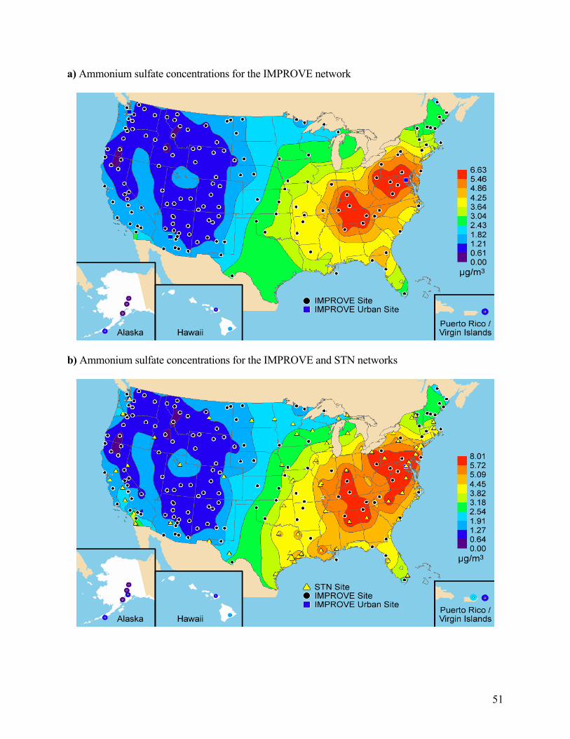
a) Ammonium sulfate concentrations for the IMPROVE network

b) Ammonium sulfate concentrations for the IMPROVE and STN networks

52

c) Ammonium sulfate fractional contribution to reconstructed fine mass for the IMPROVE network

d) Ammonium sulfate fractional contribution to reconstructed fine mass for the IMPROVE and STN networks

Figure 2.2. Isopleth maps of annual ammonium sulfate concentrations in panels a and b and percent contributions to reconstructed fine mass in panels c and d. Panels a–d include all sites from the IMPROVE network that met the prescribed completeness criteria including the urban sites from 2000–2004. Panels b and d also include all sites from the STN network that met the prescribed completeness criteria.

53

a) Total carbon concentrations for the IMPROVE network

b) Total carbon concentrations for the IMPROVE and STN networks

Figure 2.3. Isopleth maps of annual total carbon concentrations. Panels a and b include all sites from the IMPROVE network that met the prescribed completeness criteria including the urban sites for 2000–2004. Panel b also includes all sites from the STN network that met the prescribed completeness criteria.

54

a) Organic mass by carbon concentrations for the IMPROVE network

b) Organic mass by carbon concentrations for the IMPROVE and STN networks

55

c) Organic mass by carbon fractional contribution to reconstructed fine mass for the IMPROVE network

d) Organic mass by carbon fractional contribution to reconstructed fine mass for the IMPROVE and STN networks

Figure 2.4. Isopleth maps of annual organic carbon concentrations in panels a and b and percent contributions to reconstructed fine mass in panels c and d. Panels a–d include all sites from the IMPROVE network that met the prescribed completeness criteria including the urban sites for 2000–2004. Panels b and d also include all sites from the STN network that met the prescribed completeness criteria.

56

a) Light-absorbing carbon concentrations for the IMPROVE network

b) Light-absorbing carbon concentrations for the IMPROVE and STN networks

57

c) Light-absorbing carbon fractional contribution to reconstructed fine mass for the IMPROVE network

d) Light-absorbing carbon fractional contribution to reconstructed fine mass for the IMPROVE and STN networks

Figure 2.5. Isopleth maps of annual light-absorbing carbon concentrations in panels a and b and percent contributions to reconstructed fine mass in panels c and d. Panels a–d include all sites from the IMPROVE network that met the prescribed completeness criteria including the urban sites for 2000–2004. Panels b and d also include all sites from the STN network that met the prescribed completeness criteria.

58

a) Ammonium nitrate concentrations for the IMPROVE network

b) Ammonium nitrate concentrations for the IMPROVE and STN networks

59

c) Ammonium nitrate fractional contribution to reconstructed fine mass for the IMPROVE network

d) Ammonium nitrate fractional contribution to reconstructed fine mass for the IMPROVE and STN networks

Figure 2.6. Isopleth maps of annual ammonium nitrate concentrations in panels a and b and percent contributions to reconstructed fine mass in panels c and d. Panels a–d include all sites from the IMPROVE network that met the prescribed completeness criteria including the urban sites for 2000–2004. Panels b and d also include all sites from the STN network that met the prescribed completeness criteria.

60

a) Fine soil concentrations for the IMPROVE network

b) Fine soil concentrations for the IMPROVE and STN networks

61

c) Fine soil fractional contribution to reconstructed fine mass for the IMPROVE network

d) Fine soil fractional contribution to reconstructed fine mass for the IMPROVE and STN networks

Figure 2.7. Isopleth maps of annual soil concentrations in panels a and b and percent contributions to reconstructed fine mass in panels c and d. Panels a–d include all sites from the IMPROVE network that met the prescribed completeness criteria including the urban sites for 2000–2004. Panels b and d also include all sites from the STN network that met the prescribed completeness criteria.

62

a) Reconstructed fine mass for the IMPROVE network

b) Reconstructed fine mass for the IMPROVE and STN networks

Figure 2.8. Isopleth maps of annual reconstructed fine mass concentrations. Panels a and b include all sites from the IMPROVE network that met the prescribed completeness criteria including the urban sites for 2000–2004. Panel b also includes all sites from the STN network that met the prescribed completeness criteria.

63

Figure 2.9. Isopleth map of annual coarse mass concentrations; includes all sites from the IMPROVE network that met the prescribed completeness criteria including the urban sites for 2000–2004.

2.5 SPATIAL TRENDS IN PARTICULATE EXTINCTION IN THE UNITED STATES

Spatial patterns in the reconstructed particulate extinction were similar to those observed for aerosol concentrations since reconstructed particle extinction is calculated from aerosol concentrations. However, because specific scattering of sulfates and nitrates were larger than other fine aerosols because of associated water, light-absorbing carbon has relatively high specific extinction, and coarse particle scattering contributes to total particulate extinction, the extinction budgets are somewhat different from fine aerosol budgets. Total particulate extinction was not calculated for the STN, and therefore fractional contributions to total particulate extinction were also not calculated for the STN because CM is not measured by this network.

2.5.1 Fine Particle Ammonium Sulfate Extinction

Figure 2.10 shows the ammonium sulfate light extinction coefficient averaged over the 5-year period 2000–2004 and the fractional contribution of ammonium sulfate to total particulate extinction expressed as a percentage for the same period. The spatial patterns in extinction and mass concentration attributed to ammonium sulfate were very similar but with steeper gradients observed in extinction. The east-to-west gradient in ammonium sulfate extinction is even stronger than that for concentrations, with extinction coefficients in the central eastern United States over a factor of 12 higher than the low extinction values found at the interior West sites rather than the factor of 8 observed in mass concentrations.

64

Both the peak ammonium sulfate mass concentration and extinction coefficient occurred at the STN southwestern Pennsylvania site. Similar to ammonium sulfate concentrations, the highest annual average rural and urban ammonium sulfate extinction coefficients, between 60 and 75 Mm-1, were found in the central eastern United States. Extinction coefficients decrease in all directions from the high coefficient region, with extinction coefficients less than 5 Mm-1 through much of the interior West (Appendix A). The exception in the interior West is the urban Wasatch Front site, where the extinction coefficient was 12 Mm-1. Along the Pacific coast, rural extinction coefficients were typically in the 5–10 Mm-1 range, with a few rural sites in the 10–20 Mm-1 range. Urban sites along the Pacific Coast were in the 15–25 Mm-1 range.

In the East, ammonium sulfate contributes at least 50% to reconstructed particulate extinction at most IMPROVE sites, with contributions of 70–80% in the Appalachian region (Figure 2.10b) and Hawaii. Ammonium sulfate contributions to particulate extinction were between 10% and 20% at four rural sites in the West including Yosemite National Park, California; Sawtooth National Forest, Idaho; Monture, Montana; and Sycamore Canyon, Arizona, as well as Phoenix, Arizona, an urban site, and Spokane, Washington, a heavily influenced rural site. Typical contributions in the interior West were 20–30%. Sites along the Pacific coast and in the middle of the United States had intermediate ammonium sulfate contributions of 30–50%.

2.5.2 Fine Particle Carbon Extinction

Figure 2.11 shows isopleths of the light extinction attributed to organic carbon and the fractional contribution of organics to particulate extinction. Because no humidity dependence for organics was considered, the spatial trends in organic carbon extinction coefficients were the same as for mass concentrations. The largest region of high rural organic carbon extinction coefficients (12–18 Mm-1) was the southeastern United States; coefficients in this range were also present in the Sierra Nevada region of California and in the northern Rockies of Montana (Appendix A). The urban sites in the southeastern United States and California have OMC extinction coefficients that were even higher than the surrounding rural areas, with extinction coefficients greater than 18 Mm-1 at most urban sites and a peak value of 50 Mm-1 in the San Joaquin Valley of California. Additional localized high concentration areas in the Northwest, the interior West, and the midwestern United States were identified with the inclusion of the urban sites. The lowest extinction coefficients (1.5–4 Mm-1) were at the sites with the lowest OMC concentrations, which were Simeonof and Tuxedni, Alaska; Hawaii Volcanoes National Park and Haleakala, Hawaii; the Virgin Islands; Wheeler Peak, New Mexico; White River, Colorado; and White Pass, Washington.

With the exception of two sites in Arizona, Sycamore Canyon and Saguaro National Monument East, the contribution of OMC to reconstructed particulate extinction at IMPROVE sites is less than its contribution to RCFM. The greatest contributions of organic carbon to particulate extinction occur in the northwestern United States, with peak contributions of 50–60% of extinction at Trinity, Lassen Volcanic National Park, and Crater Lake National Park in the Oregon/northern California region; at Sula Peak and Monture in the northern Rockies of Montana; at Denali National Park in Alaska; and at Sawtooth National Forest in the Hells Canyon region of Idaho. Most sites in the interior mountainous West, including the northern Sierra Nevada, have extinction contributions in the 30–50% range. The remaining areas west of

65

the eastern border of Colorado were typically in the 20–30% isopleth, whereas most sites east of that line were in the 10–20% isopleth. The only site where organics contributed less than 10% to particulate extinction was the Virgin Islands.

The light extinction attributed to aerosol absorption by light-absorbing carbon and the fractional contribution of LAC to particulate extinction are shown in Figure 2.12. Again, because there is no humidity dependence for estimating the extinction attributed to LAC, the spatial trends in LAC extinction and concentration were the same. Peak rural LAC concentrations and extinction coefficients were found at Old Town, Maine; M.K. Goddard, Pennsylvania; Mingo, Missouri; and James River Face Wilderness, Virginia. The highest LAC extinction coefficients and concentrations were found at the STN sites in southeastern Florida, El Paso, Texas, New Jersey, and Puerto Rico. Unlike OMC, the percent contributions of LAC to particulate bext were, with the exception of Simeonof, Alaska, greater than their contributions to RCFM. The peak LAC extinction coefficients were primarily in the eastern United States, whereas the peak contributions to particulate bext were found in the West.

2.5.3 Fine Particle Ammonium Nitrate Extinction

Similar to ammonium sulfate, the hygroscopicity of ammonium nitrate is also accounted for in the ammonium nitrate extinction coefficients; thus the spatial trends in ammonium nitrate extinction coefficients were generally the same but not identical to those in ammonium nitrate concentrations. The isopleths of ammonium nitrate extinction coefficients and the fractional contribution of ammonium nitrate to particulate bext expressed as a percentage are shown in Figure 2.13. Rural ammonium nitrate extinction coefficients were highest at the central and southern California sites and in the Midwest, where ammonium nitrate concentrations were highest, and lowest in the interior West, where again the concentrations were lowest (Appendix A). Whereas the rural extinction coefficients were highest, 20–27 Mm-1, in the Midwest, the highest urban extinction coefficients, between 60 and 90 Mm-1, were in metropolitan Los Angeles and the San Joaquin Valley, California. Outside of the Midwest and California, the Wasatch Front in Utah was the only site to have ammonium nitrate extinction coefficients greater than 30 Mm-1. Also, similar to ammonium sulfate, there is a stronger gradient between the lowest to the highest coefficients observed at the rural sites, with a factor of 20 range in coefficients as compared to a factor of 13 observed in concentrations.

Ammonium nitrate consistently makes larger contributions, in the range of 1–7 percentage points, to particulate bext than to RCFM at the IMPROVE sites. The peak ammonium nitrate contribution to reconstructed particulate extinction of 40% is found in the San Gorgonio Wilderness, California. Contributions of greater than 30% were also found at Point Reyes National Seashore, Joshua Tree National Park, and San Gabriel, California; Lake Sugema and Viking Lake, Iowa; Great River Bluffs and Blue Mounds, Minnesota; and Columbia River Gorge, Washington.

2.5.4 Fine Particle Soil Extinction

Figure 2.14 shows the annual average spatial distribution for the 2000–2004 period of fine soil mass extinction coefficients and the soil fractions of total particulate extinction. The spatial trends in fine soil extinction are identical to the spatial trends in fine soil mass

66

concentrations—fine soil is assumed to be nonhygroscopic and its mass scattering efficiency is estimated to be 1 m2/g. To reiterate from section 2.4, the highest rural fine soil concentrations, and therefore extinction coefficients, not surprisingly were found in the arid Southwest at Sycamore Canyon and the west and east units of Saguaro National Park, Arizona, at 2.61, 3.08, and 2.18 Mm-1, respectively (Appendix A). The Virgin Islands, the Queen Valley in southern Arizona, and the west Texas sites of Guadalupe Mountains and Salt Creek all had coefficients in the 1.5–2 Mm-1 range. Rural fine soil extinction coefficients in the range of 1–1.5 Mm-1 were found in southern Colorado; the Death Valley National Monument, California; El Dorado Springs, Missouri; in the Cherokee Nation, Oklahoma; and throughout most of Arizona. For most of the rural United States, soil extinction coefficients were between 0.5 and 1 Mm-1, with the Great Lakes area, the northern Rockies, Alaska, Hawaii, and the northwestern and northeastern United States generally having soil concentrations less than 0.5 Mm-1. The peak soil extinction of 4.8 Mm-1 occurs at the urban STN site in El Paso, Texas. The STN Puerto Rico site and the IMPROVE Phoenix and Spokane sites have soil coefficients greater than 2 Mm-1. Urban soil extinction coefficients in the range of 1–2 Mm-1 are found in Arizona and west Texas, as well as in Alabama, California, Colorado, Florida, Missouri, Nebraska, and Ohio.

Whereas fractional fine soil contributions to RCFM were as high as 50%, contributions to particulate bext were all under 12%. In all cases, the contribution of fine soil to reconstructed particulate extinction is significantly less than its contribution to fine mass. In the most extreme example, fine soil contributed 51% to RCFM but only 9% to particulate bext at the Virgin Islands site. The largest contributions of fine soil to particulate bext, between 5% and 12%, were in the arid southwestern United States and the Virgin Islands.

2.5.5 Coarse Mass Particle Extinction

Figure 2.15 shows the CM extinction coefficients and the CM fractions of reconstructed extinction expressed as a percentage of particulate bext. Coarse mass is assumed to be composed of soil and to be nonhygroscopic and therefore to have an estimated mass scattering efficiency of 0.6 m2/g. The spatial trends in CM were the same as for CM concentrations and were quite distinct from the spatial trends in RCFM (see section 2.4). The highest CM concentrations, and therefore CM extinction coefficients, 5–9 Mm-1, were concentrated farther west in the middle of the United States and in the arid Southwest and southern California (Appendix A). Coarse mass extinction coefficients were also very high, 8.02 Mm-1

, in the Virgin Islands. From the central Great Plains, CM coefficients trended toward increasingly lower coefficients in the range of 1–4 Mm-1 to the north, east, and west until reaching the coasts. The sites along the Pacific, Gulf, and Atlantic coasts typically had moderate to high CM coefficients in the 3–4 Mm-1 range. The CM coefficients were generally very low, 0.5–1.5 Mm-1, in the following northwestern regions—the northern Rockies, Oregon and northern California, the Northwest, and Alaska. Similarly, low coefficients also occurred at Hawaii Volcanoes National Park, Hawaii; Shining Rock Wilderness, North Carolina; Lye Brook Wilderness, Vermont; and Seney, Michigan. The most significant contribution from CM to particulate bext, 35.7%, occured at the Virgin Islands. Contributions of 20–30% were found in Death Valley, California, western Texas, and southern Arizona. Moving from this region, west to the California coast and north to increasingly higher latitudes and moving farther inland, CM contributes between 10% and 20% to reconstructed particulate extinction. Throughout most of the Northwest and all of the eastern United States, CM contributions were less than 10%.

67

2.5.6 Total Reconstructed Particulate Extinction (bext)

Total reconstructed particulate extinction was not calculated for the STN because CM is not measured by this network. The highest rural particulate bext coefficients, those greater than 90 Mm-1, were concentrated in the central eastern United States (Figure 2.16) and the lowest, those less than 15 Mm-1, were concentrated in the interior West and Alaska (Appendix A). The high particulate bext region represents the intersect of the regions of high mass concentrations of ammonium sulfate, ammonium nitrate, OMC, and LAC in a region of comparatively high average relative humidity. The spatial trends in bext were very similar to those in RCFM; however, the east-to-west gradient between the lowest values in the interior West and the highest values in the East is stronger for the extinction coefficients (over a factor of 9 change) than for mass concentrations (over a factor of 7).

2.5.7 Visibility Expressed in Deciviews

Another way of displaying visibility estimates from aerosol data is by using the deciview (dv) scale. The dv scale was designed to linearly relate to humanly perceived differences in visibility, which is not the case for light extinction. Particle-free or Rayleigh conditions have a dv value of 0, and a change of 1 dv is a small but often noticeable change in perceived visibility.

Figure 2.17 shows isopleths of dv averaged over the 2000–2004 period. While the spatial patterns in visibility impairment were the same as for reconstructed particulate extinction, taking the log of aerosol extinction to calculate the dv has the effect of reducing the strength of the observed east-to-west gradient in dv as compared to Mm-1. The broad region that includes the Great Basin, most of the Colorado Plateau, and portions of the Rocky Mountains and Hells Canyon had visibility impairment of less than 10 dv (Appendix A). Moving in any direction from this region generally results in a gradient of increasing dv. The Alaska sites also had visibility impairment of 10 dv or less. Hawaii and the Virgin Islands were in the 10–12 dv range. Visibility impairments of 10–15 dv were found throughout much of the remainder of the West and in the Boundary Waters area. The Columbia River Gorge in Washington, San Gorgonio, Agua Tibia, and Sequoia National Park in California, and the western urban sites all had the highest visibility impairments for the West of 10–20 dv. With the exception of the Boundary Waters area, the eastern United States had visibility impairments of greater than 15 dv. The highest annual dv value was reported at Mammoth Cave National Park and Washington, D.C., with an impairment of 24 dv.

68

a) Ammonium sulfate extinction for the IMPROVE network

b) Ammonium sulfate extinction for the IMPROVE and STN networks

69

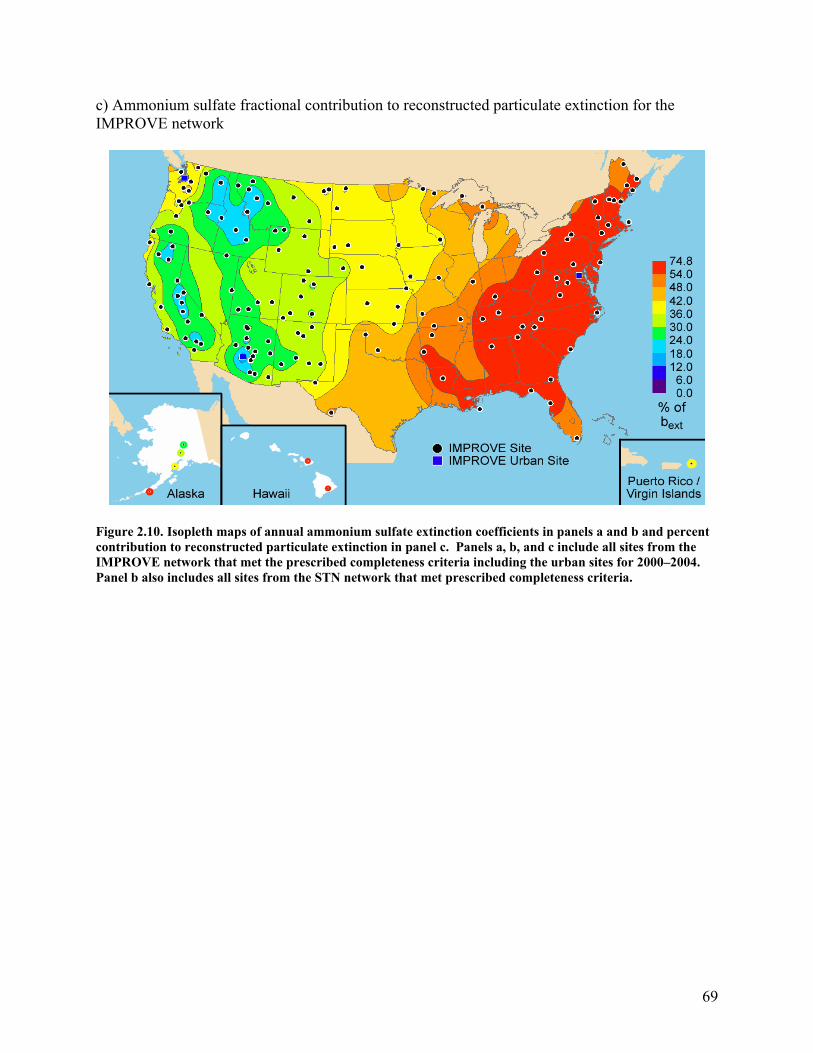
c) Ammonium sulfate fractional contribution to reconstructed particulate extinction for the IMPROVE network

Figure 2.10. Isopleth maps of annual ammonium sulfate extinction coefficients in panels a and b and percent contribution to reconstructed particulate extinction in panel c. Panels a, b, and c include all sites from the IMPROVE network that met the prescribed completeness criteria including the urban sites for 2000–2004. Panel b also includes all sites from the STN network that met prescribed completeness criteria.

70

a) Organic carbon extinction for the IMPROVE network

b) Organic carbon extinction for the IMPROVE and STN networks

71

c) Organic carbon fractional contribution to reconstructed particulate extinction for the IMPROVE network

Figure 2.11. Isopleth maps of annual organic mass by carbon extinction coefficients in panels a and b and percent contribution to reconstructed particulate extinction in panel c. Panels a, b, and c include all sites from the IMPROVE network that met the prescribed completeness criteria including the urban sites for 2000–2004. Panel b also includes all sites from the STN network that met prescribed completeness criteria.

72

a) Light-absorbing carbon extinction for the IMPROVE network

b) Light-absorbing carbon extinction for the IMPROVE and STN networks

73

c) Light-absorbing carbon fractional contribution to reconstructed particulate extinction for the IMPROVE network

Figure 2.12. Isopleth maps of annual light-absorbing carbon extinction coefficients in panels a and b and percent contribution to reconstructed particulate extinction in panel c. Panels a, b, and c include all sites from the IMPROVE network that met the prescribed completeness criteria including the urban sites for 2000–2004. Panel b also includes all sites from the STN network that met prescribed completeness criteria.

74

a) Ammonium nitrate extinction for the IMPROVE network

b) Ammonium nitrate extinction for the IMPROVE and STN networks

75

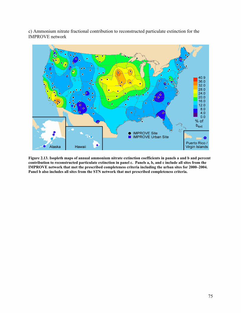
c) Ammonium nitrate fractional contribution to reconstructed particulate extinction for the IMPROVE network

Figure 2.13. Isopleth maps of annual ammonium nitrate extinction coefficients in panels a and b and percent contribution to reconstructed particulate extinction in panel c. Panels a, b, and c include all sites from the IMPROVE network that met the prescribed completeness criteria including the urban sites for 2000–2004. Panel b also includes all sites from the STN network that met prescribed completeness criteria.

76

a) Fine soil extinction for the IMPROVE network

b) Fine soil extinction for the IMPROVE and STN networks

77

c) Fine soil fractional contribution to reconstructed particulate extinction for the IMPROVE network

Figure 2.14. Isopleth maps of annual fine soil extinction coefficients in panels a and b and percent contribution to reconstructed particulate extinction in panel c. Panels a, b, and c include all sites from the IMPROVE network that met the prescribed completeness criteria including the urban sites for 2000–2004. Panel b also includes all sites from the STN network that met prescribed completeness criteria.

78

a) Coarse mass extinction for the IMPROVE network

b) Coarse mass contribution to reconstructed particulate extinction for the IMPROVE network

Figure 2.15. Isopleth maps of annual coarse mass extinction coefficients in panel a and percent contribution to reconstructed particulate extinction in panel b. Panels a and b include all sites from the IMPROVE network that met the prescribed completeness criteria including the urban sites for 2000–2004.

79

Figure 2.16. Isopleth map of annual total reconstructed particulate extinction in panel a. Includes all sites from the IMPROVE network that met the prescribed completeness criteria including the urban sites for 2000–2004. Rayleigh scattering was not included.

Figure 2.17. Isopleth map of annual visibility in deciviews in panel a. Includes all sites from the IMPROVE network that met the prescribed completeness criteria including the urban sites for 2000–2004.

80

REFERENCES

Bond, T. C., and R. W. Bergstrom (2005), Light absorption by carbonaceous particles: An investigative review, Aerosol Science and Technology, 39, 1-41.

Chu, S.-H. (2004), PM2.5 episodes as observed in the speciation trends network, Atmos. Environ., 38, 5237-5246.

Day, D. E., W. C. Malm, and S. M. Kreidenweis (1997), Seasonal variations in aerosol composition and acidity at Shenandoah and Great Smoky Mountains National Park, J. Air & Waste Manage. Assoc., 47, 411-418.

Day, D. E., W. C. Malm, and S. M. Kreidenweis (2000), Aerosol light scattering measurements as a function of relative humidity, J. Air & Waste Manage. Assoc., 5169-5176.

DeBell, L. J., M. Vozzella, R. W. Talbot, and J. E. Dibb (2004), Asian dust storm events of 2001 and associated pollutants observed in New England by the Atmospheric Investigation, Regional Modeling, Analysis and Prediction (AIRMAP) monitoring network, J. Geophys. Res., 109, D01304, doi:10.1029/2003JD003733.

Gebhart, K. A., and W. C. Malm (1989), An investigation of the size distributions of particulate sulfate concentrations measured during WHITEX, In Transactions of the AWMA/EPA Int’l Specialty Conference on Visibility and Fine Particles, edited by C.V. Mathai, Air and Waste Management Association, 157-169.

Gebhart, K. A., W. C. Malm, and D. E. Day (1994), Examination of the effects of sulfate acidity and relative humidity on light scattering at Shenandoah National Park, Atmos. Environ., 28(5), 841-849.

Grosjean, D., and S. K. Friedlander (1975), Gas-particle distribution factors for organics and other pollutants in the Los Angeles atmosphere, J. Air Pollution Control Assoc., 25, 1038-1044.

Hand, J. L., R. B. Ames, S. M. Kreidenweis, D. E. Day, and W. C. Malm (2000), Estimates of particle hygroscopicity during the Southeastern Aerosol and Visibility Study, J. Air & Waste Manage. Assoc., 50, 677-685.

Hand, J. L., S. M. Kreidenweis, D. E. Sherman, J. L. Collett, Jr., S. V. Hering, D. E. Day, and W. C. Malm (2002), Aerosol size distributions and visibility estimates during the Big Bend Regional Aerosol Visibility and Observational Study (BRAVO), Atmos. Environ., 36, 5043-5055.

Hand, J. L., and W. C. Malm (2006), Review of the IMPROVE equation for estimating ambient light extinction coefficients, http://vista.cira.colostate.edu/improve/Publications/GrayLit/016_IMPROVEeqReview/IMPROVEeqReview.htm

81

Hatakeyama, S., K. Izumi, T. Fukuyama, and H. Akimoto (1989), Reactions of ozone with alpha-pinene and beta-pinene in air: Yields of gaseous and particulate products, J. Geophys. Res., 94, 13,013-13,024.

Hawthorne, S. B., D. J. Miller, J. J. Langenfeld, and M. S. Krieger (1992), PM10 to high volume collection and quantification of semi- and nonvolatile phenols, methoxylated phenols, alkanes, and polycyclic aromatic hydrocarbons from winter urban air and their relationship to wood smoke, Environ. Sci. Technol., 26, 2251-2283.

Hogrefe O., J. J. Schwab, F. Drewnick, G. G. Lala, S. Peters, K. J. Demerjian, K. Rhoads, H. D. Felton, O. V. Rattigan, L. Husain, and V. A. Dutkiewicz (2004), Semicontinuous PM2.5 sulfate and nitrate measurements at an urban and rural location in New York: PMTACS-NY summer 2001 and 2002 campaigns, J. Air & Waste Manage. Assoc., 54, 1040-1060.

Holes, A., A. Esebi, D. Grosgean, and D. Allen (1997), FTIR analysis of aerosol formed in the presence of the photo oxidation of 1,2,4–trimethylbenene, Aerosol Sci. Technol., 26, 516–526.

IMPROVE technical subcommittee for algorithm review (2006), Revised IMPROVE Algorithm for Estimating Light Extinction from Particle Speciation Data, http://vista.cira.colostate.edu/improve/Publications/GrayLit/019_RevisedIMPROVEeq/RevisedIMPROVEAlgorithm3.doc.

Izumi, K., and T. Fukuyama (1990), Photochemical aerosol formation from aromatic hydrocarbons in the presence of NOx, Atmos. Environ., Part A, 241, 1433-1441.

Jaffe, D., J. Snow, and O. Cooper (2003), The April 2001 Asian dust events: transport and substantial impact on surface particulate matter concentrations across the United States, EOS transactions, November 18.

Jang, M., and R. M. Kamens (1999), Newly characterized products and composition of secondary aerosols from the reaction of alpha-pinene with ozone, Atmos. Environ., 33, 459-474.

Jang, M., and R. M. Kamens (2001), Atmospheric secondary aerosol formation by heterogeneous reactions of aldehydes in the presence of a sulfuric acid aerosol catalyst, Environ. Sci. Technol., 35, 4758-4766.

Kavouras, I. G., N. Mihalopoulos, and E. G. Stephanou (1998a), Formation of atmospheric particles from organic acids produced by forests, Nature, 395, 683-686.

Kavouras, I. G., N. Mihalopoulos, and E. G. Stephanou (1998b), Secondary aerosol formation vs. primary organic aerosol emission: In situ evidence for chemical coupling between monoterpene acid photochemical products and new particle formation over forests, Environ. Sci. Technol., 33, 1028-1037.

82

Lee, T., S. M. Kreidenweis, and J. L. Collett, Jr. (2004), Aerosol ion characteristics during the Big Bend Regional Aerosol and Visibility Observational Study, J. Air & Waste Manage. Assoc., 54, 585-592.

Lefer, B. L., and R. W. Talbot (2001), Summertime measurements of aerosol nitrate and ammonium at a northeastern U.S. site, J. Geophys. Res., 106(D17), 20365-20378.

Liu L.-J. S., R. Burton, W. E. Wilson, and P. Koutrakis (1996), Comparison of aerosol acidity in urban and semi-rural environments, Atmos. Environ., 30(8), 1237-1245.

Lowenthal, D.H., C. F. Rogers, P. Saxena, J. G. Watson, and J. C. Chow (1995), Sensitivity of estimated light extinction coefficients to model assumptions and measurement errors, Atmos. Environ., 29, 751-766.

Lowenthal, D. H., J. G. Watson, and P. Saxena (2000), Contributions to light extinction during project MOHAVE, Atmos. Environ., 34, 2351-2359.

Malm, W. C., H. Iyer, J. Watson, and D. A. Latimer (1989), Survey of a variety of receptor modeling techniques, In Transactions of the AWMA/EPA Int’l Specialty Conference on Visibility and Fine Particles, edited by C.V. Mathai, Air and Waste Management Association.

Malm, W. C., J. F. Sisler, D. Huffman, R. A. Eldred, and T. A. Cahill (1994), Spatial and seasonal trends in particle concentration and optical extinction in the United States, J. Geo. Res., 99(D1), 1347-1370.

Malm, W. C., and S. M. Kreidenweis (1997), The effects of models of aerosol hygroscopicity on the apportionment of extinction, Atmos. Environ., 31, 1965-1976.

Malm, W. C., D. E. Day, and S. M. Kreidenweis (1997), Comparison of measured and reconstructed scattering during an intensive field study at Great Smoky Mountains National Park, paper #97-WA70.02, presented at the Air and Waste Management 90th Annual Meeting, Pittsburgh, PA.

Malm, W. C. (1998), Examining the relationship between aerosol concentration and partial scattering efficiencies near the Grand Canyon, Presented at the 91st Annual Meeting of the Air and Waste Management Association, Pittsburgh, PA.

Malm, W. C., D. E. Day, and S. M. Kreidenweis (2000a), Light scattering characteristics of aerosols at ambient and as a function of relative humidity: part II---a comparison of measured scattering and aerosol concentrations using statistical models. J. Air and Waste Management Association, 50, 174-182.

Malm, W. C., J. F. Sisler, M. L. Pitchford, M. Scruggs, R. Ames, S. Copeland, K. A. Gebhart, and D. E. Day (2000b), Spatial and seasonal patterns and temporal variability of haze and its constituents in the United States: Report III, Cooperative Institute for Research in the Atmosphere, Colorado State University, ISSN 0737-5352-47.

83

Malm, W. C., B. A. Schichtel, R. B. Ames, and K. A Gebhart (2002), A 10-year spatial and temporal temporal trend of sulfate across the United States, J. Geo. Res., 107(D22), 4627, doi:10.1029/2002JD002107.

Malm W. C., D. E. Day, S. M. Kreidenweis, J. L. Collett, Jr., T. Lee (2003), Humidity dependent optical properties of fine particles during the Big Bend Regional Aerosol and Visibility Observational study (BRAVO), J. Geophys. Res. 108(D9), 4279, doi:10.1029/2002JD002998.

Malm W. C, B. A. Schichtel, M. L. Pichford, L. L. Ashbaugh, and R. A. Eldred (2004), Spatial and monthly trends in fine particle concentration in the United States, J. Geophys. Res. 109, D03306, doi:10.1029/2003JD003739.

Malm W. C., D. E. Day, C. Carrico, S. M. Kreidenweis, J. L. Collett, Jr., G. McMeeking, T. Lee, and J. Carrillo (2005), Inter-comparison and closure calculations using measurements of aerosol species and optical properties during the Yosemite Aerosol Characterization Study, J. Geophys. Res., 110, D14.

Malm, W. C., M. L. Pitchford, C. McDade, and L. L. Ashbaugh (2006), Coarse particle speciation at selected locations in the rural continental United States, Atmos. Environ, accepted.

Odum, J. R., T. Hoffmann, F. Bowman, D. Collins, R. C. Flagan, and J. H. Seinfeld (1996), Gas/particle partitioning and secondary organic aerosol yields, Environ. Sci. Technol., 30, 2580-2585.

Odum, J. R., P. W. Jungkamp, R. J. Griffin, H. J. L. Forstner, R. C. Flagan, and J. H. Seinfeld (1997), Aromatics, reformulated gasoline, and atmospheric organic aerosol formation, Environ. Sci. Technol., 31, 1890-1897.

Ouimette, J. R., and R. C. Flagan (1982), The extinction coefficient of multicoponent aerosols, Atmos. Environ., 16, 2405.

Perry, K. D., T. A. Cahill, R. A. Eldred, and D. D. Dutcher (1997), Long-range transport of North African dust to the eastern United States, J. Geophys. Res., 102(D10), 11225-11238.

Pitchford, M. L., and W. C. Malm (1994), Development and applications of a standard visual index, Atmos. Environ., 28(5), 1049-1054.

Prospero, J. M. (1999), Long-term measurements of the transport of African mineral dust to the southeastern United States: Implications for regional air quality, J. Geophys. Res., 104(D13), 15,917-15,927.

Rogge, W. F., L. M. Hildemann, M. A. Mazurek, G. R. Cass, and B. R. T. Simoneit (1996), Mathematical modeling of atmospheric fine particle associated primary organic compound concentrations, J. Geophys. Res., 101, 19,379-19,394.

84

Quinn, P. K., T. L. Miller, T. S. Bates, J. A. Ogren, E. Andrews, and G. E. Shaw (2002), A 3-year record of simultaneously measured aerosol chemical and optical properties at Barrow, Alaska, J. Geophys. Res., 107(D11), 4130, 10:1029/2001JD001248.

Schmidt, K. M., J. P. Menakis, C. C. Hardy, W. J. Hann, and D. L. Bunnell (2002), Development of course-scale spatial data for wildland fire and fuel management, Gen. Tech. Rep. RMRS-87, USDA For. Serv. Rocky Mt. Res. Stn., Fort Collins, Colo.

Schwab, J. J., H. D. Felton, and K. L. Demerjian (2004), Aerosol chemical composition in New York state from integrated filter samples: Urban/rural and seasonal contrasts, J. Geophys. Res., 109(D16S05), doi:10.1029/2003JD004078.

Sloane C. S. (1983), Optical properties of aerosols-comparison of measurements with model calculations, Atmos. Environ., 17, 409-416.

Sloane C. S. (1984), Optical properties of aerosols of mixed composition, Atmos. Environ., 18, 871-878.

Sloane C. S., and G. T. Wolff (1985), Change in aerosol optical properties with change in chemical composition, Atmos. Environ., 19, 669-680.

Sloane C.S. (1986), Effects of composition on aerosol light scattering efficiencies, Atmos. Environ., 20, 1025.

Tang, I. N. (1996), Chemical and size effects of hygroscopic aerosols on light scattering coefficients, J. Geophys. Res., 101(D14), 19245-19250.

Tanner, R. L., W. J. Parkhurst, M. L. Valente, and W. D. Phillips (2004), Regional composition of PM2.5 aerosols measured at urban, rural, and “background” sites in the Tennessee valley, Atmos. Environ., 38, 3143-3153.

Turpin, B. J., and H. J. Lin (2001), Species contributions to PM2.5 mass concentrations: Revisiting common assumptions for estimating organic mass, Aerosol Science and Technology, 35, 602-610.

U.S. EPA (2000), National Air Pollutant Emissions Trends, 1900-1998, Office of Air Quality Planning and Standards, EPA-454/R-00-002.

U.S. EPA (2003), Guidance for Tracking Progress Under the Regional Haze Rule, Contract No. 68-D-02-0261, Work Order No. 1-06.

VanCuren, R. A., and T. A. Cahill (2002), Asian aerosols in North America: Frequency and concentration of fine dust, J. Geophys. Res., 107(D24), 4804, doi:10.1029/2002JD002204.

VanCuren, R. A. (2003), Asian aerosols in North America: Extracting the chemical composition and mass concentration of the Asian continental aerosol plume from long-term aerosol records in the western United States, J. Geophys. Res., 108(D20), 4623, doi:10.1029/2003JD003459.

85

van de Hulst, H. C. (1981), Light Scattering by Small Particles, Dover Publications, New York.

Waggoner, A. P., R. E. Weiss, N. C. Ahlquist, D. S. Covert, S. Will, and R. J. Charlson (1981), Optical characteristics of atmospheric aerosols, Atmos. Environ., 15, 1891-1909.

Wexler, A., and J. Seinfeld (1991),Second-generation inorganic aerosol model, Atmos. Environ., 25A, 2731.

White, W. H., and P. T. Roberts (1977), On the nature and origins of visibility-reducing aerosols in the Los Angels Air Basin, Atmos. Environ., 11, 803-812.

Zhang, Q., M. R. Canagaratna, J. T. Jayne, D. R. Worsnop, and J.-L. Jimenez (2005), Time- and size-resolved chemical composition of submicron particles in Pittsburgh: Implications for aerosol sources and processes, J. Geophys. Res., 110, D07S09, doi:10.1029/2004JD004649.