estimation and optimal configurations for localization

LUND UNIVERSITY

PO Box 117221 00 Lund+46 46-222 00 00

Estimation and Optimal Configurations for Localization Using Cooperative UAVs

Purvis, Keith B.; Åström, Karl Johan; Khammash, Mustafa

Published in:IEEE Transactions on Control Systems Technology

2008

Link to publication

Citation for published version (APA):Purvis, K. B., Åström, K. J., & Khammash, M. (2008). Estimation and Optimal Configurations for LocalizationUsing Cooperative UAVs. IEEE Transactions on Control Systems Technology, 16(5), 947-958.

Total number of authors:3

General rightsUnless other specific re-use rights are stated the following general rights apply:Copyright and moral rights for the publications made accessible in the public portal are retained by the authorsand/or other copyright owners and it is a condition of accessing publications that users recognise and abide by thelegal requirements associated with these rights. • Users may download and print one copy of any publication from the public portal for the purpose of private studyor research. • You may not further distribute the material or use it for any profit-making activity or commercial gain • You may freely distribute the URL identifying the publication in the public portal

Read more about Creative commons licenses: https://creativecommons.org/licenses/Take down policyIf you believe that this document breaches copyright please contact us providing details, and we will removeaccess to the work immediately and investigate your claim.

Download date: 13. Mar. 2022

https://portal.research.lu.se/en/publications/e89a6e16-3d0c-40b4-a054-f18c49fd2341

IEEE TRANSACTIONS ON CONTROL SYSTEMS TECHNOLOGY, VOL. 16, NO. 5, SEPTEMBER 2008 947

Estimation and Optimal Configurations forLocalization Using Cooperative UAVs

Keith B. Purvis, Member, IEEE, Karl J. Åström, Fellow, IEEE, and Mustafa Khammash, Fellow, IEEE

Abstract—The time-difference of arrival techniques are adaptedto locate networked enemy radars using a cooperative team ofunmanned aerial vehicles. The team is engaged in deceiving theradars, which limits where they can fly and requires accurateradar positions to be known. Two time-differences of radar pulsearrivals at two vehicle pairs are used to localize one of the radars.An explicit solution for the radar position in polar coordinatesis developed. The solution is first used for position estimationgiven “noisy” measurements, which shows that the vehicle tra-jectories significantly affect estimation accuracy. Analyzing theexplicit solution leads to The Angle Rule, which gives the optimalvehicle configuration for the angle estimate. Analyzing the FisherInformation Matrix leads to The Coordinate Rule, which givesa different optimal configuration for the position estimate. Alinearized time-varying model is also formulated and an ExtendedKalman Filter applied. This estimation scheme is compared withthe earlier one, with the second showing overall improvement inreducing the variance of the estimate.

Index Terms—Electronic warfare, Fisher Information Matrix,Kalman filtering, localization, optimal configuration, position es-timation, unmanned aerial vehicles (UAVs).

I. INTRODUCTION

T HE Estimation Problem addressed here is connected tothe Cooperative Deception Problem in [1], [2]: using

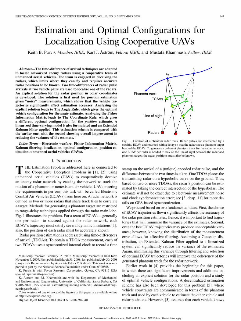
unmanned aerial vehicles (UAVs) to cooperatively deceivean enemy radar network by causing the network to track themotion of a phantom or nonexistent air vehicle. UAVs meetingthe requirements to perform this task will be called ElectronicCombat Air Vehicles (ECAVs) from here on. A radar network isdefined as two or more radars that share track files to correlatea target. Methods for generating a phantom target are restrictedto range-delay techniques applied through the radar main lobe.Fig. 1 illustrates the problem. For a team of ECAVs—generallyone per radar—to succeed against the radar network, eachECAV’s trajectory must satisfy several dynamic limitations [1];also, the position of each radar must be accurately known.

Radar position estimation is addressed using time-differencesof arrival (TDOAs). To obtain a TDOA measurement, each oftwo ECAVs uses a synchronized internal clock to record a time

Manuscript received February 15, 2007. Manuscript received in final formNovember 7, 2007. First published March 31, 2008; last published July 30, 2008(projected). Recommended by Associate Editor C. Rabbath. This work was sup-ported in part by the National Science Foundation under Grant 0300568.

K. Purvis is with Toyon Research Corporation, Goleta, CA 93117 USA(e-mail: [email protected]).

K. Åström and M. Khammash are with the Department of Mechanicaland Environmental Engineering, University of California, Santa Barbara, CA93106-5070 USA (e-mail: [email protected]; [email protected]).

Color versions of one or more of the figures in this paper are available onlineat http://ieeexplore.ieee.org.

Digital Object Identifier 10.1109/TCST.2007.916348

Fig. 1. Creation of a phantom radar track. Radar pulses are intercepted by astealthy ECAV and returned with a delay so that the radar sees a phantom targetbeyond the ECAV. To generate a coherent phantom track for the radar network,one ECAV per radar is needed to stay on the line of sight between the radar andphantom target; the radar positions must also be known.

stamp on the arrival of a (unique) encoded radar pulse, and thedifference between the two times is taken. One TDOA places thetransmitting radar on a hyperbolic curve on the ground. Thus,based on two or more TDOAs, the radar’s position can be esti-mated by taking the correct intersection of the hyperbolas. Theestimate will not be exact due to electronic measurement noiseand clock synchronization error; see [3, chap. 11] for more de-tails on GPS-based synchronization.

We proceed based on two fundamental ideas. First, the choiceof ECAV trajectories flown significantly affects the accuracy ofthe radar position estimates. Hence, it is important to find trajec-tories that will minimize the variance of the estimates. Second,even the best ECAV trajectories may produce unacceptable vari-ance; however, knowing the distribution of the measurementerror allows for effective filtering. Assuming a Gaussian dis-tribution, an Extended Kalman Filter applied to a linearizedsystem can significantly reduce the variance of the estimates.Again, minimizing this variance through filtering and selectionof optimal ECAV trajectories will improve the coherency of thegenerated phantom track for the radar network.

Earlier work in [4] provides the beginning for this paper,in which there are significant improvements and additions in-cluding an explicit solution for the radar position and a studyof optimal vehicle configurations. A decentralized estimationscheme has also been developed for this problem [5], wherevehicle constraints are communicated in terms of the phantomtrack and used by each vehicle to estimate the other vehicle andradar positions. However, [5] assumes that each vehicle knows

1063-6536/$25.00 © 2008 IEEE

Authorized licensed use limited to: Lunds Universitetsbibliotek. Downloaded on November 4, 2008 at 08:21 from IEEE Xplore. Restrictions apply.

948 IEEE TRANSACTIONS ON CONTROL SYSTEMS TECHNOLOGY, VOL. 16, NO. 5, SEPTEMBER 2008

Fig. 2. ECAV and phantom track variables. The main variables are shown forone radar and ECAV, where the ECAV is on the LOS from the radar to thegenerated phantom target.

exactly where its radar is located, whereas we drop this assump-tion as the starting point of our study.

Our goal is to determine an estimation system and op-timal vehicle configurations that will localize an emitter withminimum variance. First, we provide some background onthe cooperative deception problem. An uncertainty analysisshows how inaccurate radar position estimates will lead tomission failure. Second, we lay the framework for positioningusing TDOA measurements. By parametrizing the TDOAequations/hyperbolas in polar coordinates, we derive a novel,explicit solution for the radar position. This solution is used toperform estimation by direct calculation and time averaging.Third, we investigate optimal platform configurations that willminimize the error in the estimates. By analyzing our explicitsolution, we get The Angle Rule, and this is compared withThe Coordinate Rule via the Fisher Information Matrix. Last,we develop a linearized model for the estimation system andimplement an Extended Kalman Filter; simulations are shownand compared with the earlier scheme.

II. DECEPTION PROBLEM BACKGROUNDS

The scenarios considered herein are all constant-elevationsince the phantom will typically fly at a constant altitude, andany minor descents can be easily decoupled and handled bythe ECAVs. Assuming that an ECAV is stealthy and knows

, the maximum operational range, and the location of aradar with pulse-to-pulse agility, the ECAV can intercept andsend delayed returns of the radar’s transmitted pulses so thatthe radar sees a phantom target at a range beyond the ECAV butcloser than . To maintain deception, each ECAV behavesmuch like a bead on a string that is rotating at some variablerate; the ECAV may slide up or down freely but must rotate withthe line of sight (LOS) from the radar to the phantom track. Inother words, the ECAV has one constraint, , and one degreeof freedom over time. Fig. 2 shows the main variables and theirrelations.

The phantom track is assumed given since there are alreadymany criteria besides accurate position estimation governing itsselection [6]. Without loss of generality, is also assumed pos-itive. We use a constant-heading, constant-speed phantom trackonly for simplicity, which is given by

Fig. 3. Phantom variation due to an unknown radar location. The vehicle pro-jecting the phantom target knows its position but only has an uncertainty diskfor the radar defined by � centered at the assumed location. The worst casedeviation in phantom range and azimuth occurs when the radar is actually lo-cated at the dot on the edge of the disk.

where (see Fig. 2 for most of the variables used).The subscript 0 refers to when . To generate the phantomtrack, each ECAV flies a bearing of from its radar and usesrange-delay techniques as previously described to put a phantomtarget at the range , where indexes the ECAVs.

For this work, we put our ECAV model in the Cartesian frame:

(1)

(2)

where the control is the vehicle heading rate. The reason forusing Cartesian instead of polar coordinates is that with the posi-tion of the radar unknown, the coordinates would have anunknown origin. Based on the ECAV dynamics, is restrictedto be piecewise continuous. Since is positive,

is also required. To remain in sync with the phantomtrack, the ECAV must constantly adjust its speed as given by (2).

A. Uncertainty Analysis

Since the main reason for estimating the radar positions is tomaintain a coherent phantom track for the radar network, it isessential to examine just how much the phantom target is af-fected by an assumed radar location that is inaccurate. This in-accuracy contributes to a region of uncertainty around a nom-inal phantom target where the target may actually be placed byan unsuspecting ECAV. If the region is too large, then the net-worked radars will be able to discriminate between their respec-tively observed phantom targets and “see” through the decep-tion. Given an uncertainty in the radar location of , Fig. 3


PURVIS et al.: ESTIMATION AND OPTIMAL CONFIGURATIONS FOR LOCALIZATION USING COOPERATIVE UAVS 949

Fig. 4. Estimation of the middle radar position without noise. Three vehicles/sensors can localize a radar/emitter using two TDOA measurements. Withoutnoise, n ; n = 0, the estimate is exact.

shows the worst case situation that would produce maximumdeviation in both the range and bearing/azimuth of the phantomtarget. Using the figure as a guide, we get the following equa-tions:

(3)

(4)

With km and km, the critical radar resolu-tions for m are m in range and

in azimuth. The critical resolution for az-imuth is double that of (4) since one ECAV could be projecting

and another ; however, can only bepositive. If the radars were to have a resolution better/smallerthan the calculated resolutions, then the phantom track wouldbe dismissed as spurious. We observe that the critical range res-olution is so small as to be inconsequential; indeed, the typeof aircraft desirable for the phantom to emulate would be onthe order of tens of meters. However, the critical azimuth res-olution is significant; to get a better idea, convert to distanceat the range km, which gives 1 km for 1.91 . Thus,knowing the radar location accurately in terms of angle is im-portant, whereas range is not.

In summary, the phantom track deception can be successfulif the radar locations or angles are known. Otherwise, eachECAV’s expected placement of the phantom target may besignificantly different from its actual placement, which willresult in an incoherent phantom track for the radar network.Therefore, we proceed to find methods to accurately estimatethe radar positions.

III. RADAR POSITIONING USING TIME DIFFERENCES

We assume for now that the ECAVs know their exact po-sitions. We also assume that the ECAVs have synchronizedclocks and can detect pulses from radar side lobes, which aremuch weaker in power than those from the main lobe. Theside-lobe assumption is necessary for the ECAVs to obtain

Fig. 5. Hyperbolic bands resulting from measurement noise. White noise en-tering the TDOA measurements, n ; n 6= 0, causes a spread of hyperbolicbands, which do not exactly touch the unknown radar location. Thus, the vehi-cles seeking to localize the radar will get an inexact estimate.

TDOA measurements of radar pulses since each radar looksdirectly at only one of the ECAVs. Side lobes are normallyactively suppressed to attenuate noise leaking in from nearbysources or reflectors, so as to maximize the signal-to-noise ratiofor the signal from the main-lobe direction. However, side lobescannot be entirely eliminated, and it is much easier to receiveside lobe transmissions than it is to detect their (reflected) return( versus ). To simplify analysis, just the position ofthe middle radar—that corresponding to ECAV 2—is estimatedusing two TDOA measurements1 from ECAV pairs 1–2 and3–2. The measurements—converted to distance—are modeledby

(5)

where is the speed of light, is the measured pulse arrivaltime at the th ECAV, and and are the combined noise/error from the arrival times. The other variables are shown inFig. 4, which illustrates the ideal case when two noise-free mea-surements are used to determine the position of themiddle radar. Since and are distance differences, theynaturally give rise to hyperbolas, on which the emitting radarmust be located. With white noise added to ap-proximate the collective effect of electronic measurement noiseand clock synchronization error2 in the ’s, hyperbolic bandsare created as shown in Fig. 5. Intuitively, the variance of theposition estimates will be smaller when the ECAVs are morespread apart in angle.

Note that only and can be measured—absolute dis-tances and pulse travel times are unknown. Obtaining a givenstreams of pulse arrival times from two ECAVs requires com-munication and some signal processing to match up the twoprofiles by their corresponding encoded radar pulses. With only

1If more than two measurements are used, then the system of equations isoverdetermined, and methods such as nonlinear least squares as in [7] or Kalmanfiltering may be used to find the best “average” position estimate.

2A first-order Gauss-Markov process would be more accurate for GPS syn-chronization according to [3, Ch. 11], but a Gaussian random process is usedfor simplicity.



two TDOAs/hyperbolas, more than one intersection will resultin most cases. One of the two halves of each hyperbola can beruled out based on the signs of and (as done in Fig. 4),which leaves two intersections in general. However, the correctintersection nearest the true position of the middle radar canbe identified by discriminating the intersections as the ECAVsmove over time, or by assuming an approximate location for theradar is previously known.

There are other methods for locating emitters besides usingTDOA measurements, which include angle of arrival (AOA), re-ceived signal strength (RSS), and time of arrival (TOA) or traveltime (see [8] for more details). However, using AOA measure-ments would be less accurate than TDOA, especially given aninexpensive antenna likely for an ECAV. RSS assumes that thetransmitted power is known so that its attenuation over distancecan be computed and compared with the actual received signal,but the transmitted power is unknown in our case, and a radarcan modulate its transmitted power in normal operation. TOAintroduces a clock bias parameter and cannot be used in our casebecause the time at which a pulse leaves the radar is unknown,hence travel time cannot be determined.

IV. EXPLICIT SOLUTION FOR THE RADAR POSITION

Calculating the exact intersection of two hyperbolas is diffi-cult, and many efforts have been made to do so as outlined in [9].Here, we give an alternative solution not found in [9], which isparticularly useful for our case due to the polar parametrization.First, parametrize each hyperbola in polar coordinateswith the middle vehicle as the common origin

(6)

(7)

where and are the range and bearing, respectively, ofECAV from ECAV 2. The reason we choose ECAV 2 as theorigin for the coordinates is that it is the vehicle assigned todeceive the middle radar, and radar position estimates should berelative to the ECAV using them. As designated, the functions

and do map each angle to a unique range eventhough from a plot like Fig. 4, it might appear that using ECAV 2as the origin gives two ranges for some values of . However,one must realize that the point can also be represented by

. The emitting radar must be located on the half ofthe hyperbola having positive values for .

To form a hyperbola requires that the eccentricity begreater than one, where appears with in either (6) or (7).This gives rise to an important condition for the measurements:

(8)

If the measurement has zero noise, then condition (8) willalways be met, modulo equality when both vehicles in the pairhave the same bearing from the radar (this gives a parabola). Ifthe noise is nonzero, then (8) may be violated as ,which results in an ellipse instead of a hyperbola. Violation be-comes more likely when is small or both vehicles have sim-ilar bearings.

Equating (6) and (7) gives a trigonometric equation, whichhas two solutions for and hence for position

(9)

(10)

With zero noise, it can be shown that provided that noneof the ECAVs share the same bearing from the middle radar. Thetwo solutions for come from taking the , and this angleis always in the first quadrant for the scenarios we work with.The corresponding range can be found by substituting into(6) or (7) as shown by (10). For ECAV 2 to compute , it needsthe relative ranges and angles of the other ECAVs providingmeasurements. If there is no noise in the measurements and

, then the position estimate is exact. With noise, theestimate is only approximate.

This solution is well-suited to our application and differentfrom the many solutions in [9] because the angle of the positionestimate can be directly calculated and analyzed without firstobtaining or , which are not really needed. Specif-ically, for an ECAV generating a phantom track using range-delay techniques, the distance from the ECAV to the radaris not important, but rather the distance from the ECAV to thephantom, . As long as the latter is known, which wouldbe true with the ECAV position and phantom track known, theECAV can intercept and appropriately delay radar pulses by thedelay time , where is the speed of light. Cou-pled with an accurate angle estimate , this allows the ECAVto place a phantom target where intended without knowing howfar away the radar is (see also Fig. 3 and accompanying discus-sion). The range estimate is still useful in secondary ways andfor other problems, so it should not be disregarded entirely. It isalso used here to convert to for measuring the perfor-mance of the estimation schemes.

A. Simulations of Estimation by Direct Calculation

We now apply the results from Section IV to estimate themiddle radar position over time in a scenario with a fixedphantom track. The measurement noise is Gaussian with inten-sity 0.0001 km /Hz for both measurements, which correspondsto a -error of 30 m with a measurement taken every 0.1 s.Instead of assuming that there is no temporal correlation ofthe position, we capitalize on the stationarity of the radarand take a running average of the estimates over time. Thisstrategy is effective as long as the distribution of the estimatesis approximately normal. In this and subsequent simulations,the performance of the estimation scheme is measured by theroot mean square error (RMSE), which is defined for Cartesiancoordinates as

RMSE (11)

where and are the true coordinates of the middle radar,and and are the corresponding estimates, all relative to



Fig. 6. Estimation of the middle radar position using the explicit solution. The radar position is directly calculated and the estimates averaged over time; themeasurement noise has intensity 0.0001 km /Hz, and 1000 runs are made. The root mean square errors of the position and angle estimates are plotted as RMSEand RMSE , respectively. The only difference between the two scenarios is how far the vehicles are from the radars, which affects their relative separation anglesand hence the errors.

some fixed reference frame. We also use the RMSE for the angleestimate, which is

RMSE (12)

where is the angle of the middle radar, and is the corre-sponding estimate, all relative to a polar frame with the middlevehicle as the origin. The expectation is taken over 1000 runsunless otherwise stated.

Fig. 6 shows two scenarios where position estimation is doneby direct calculation using (9)–(10) and time averaging. Thephantom track is straight with a constant speed of 100 m/s anda length of approximately 26 km. The only difference betweenthe two scenarios is the ECAV trajectories, which are governedby (1)–(2). Both the RMSE and the RMSE are plotted foreach scenario. For each run, the measurement noise sequencesare chosen randomly.

Observing Fig. 6(a), halfway through the time intervalthe RMSE decreases to roughly 5 m and tends to leveloff as time increases. In Fig. 6(b), the RMSE decreasesto roughly 100 m and then starts increasing sharply as timeincreases. The key difference between the two scenarios, andwhat causes the RMSE to increase with time in the secondscenario, is not how far the ECAVs are from the radars buthow spread apart in angle; we will substantiate this idea inthe next section. Fig. 6 also shows that in the transient, theRMSE does not track the RMSE , although obviously

RMSE RMSE (the otherdirection does not hold).

V. OPTIMAL VEHICLE CONFIGURATIONS

Fig. 6 suggests that the estimation error is lower when thevehicles are sufficiently spread apart in angle, and we formally

pursue this idea. The explicit solution from Section IV is used todetermine vehicle configurations that minimize the sensitivity ofthe estimate to measurement noise, and this gives The AngleRule. The Fisher Information Matrix also gives an additionalperspective, and by it we get The Coordinate Rule. Combinedtogether, these results provide an understanding for how the op-timal configurations depend on the form of the estimate one isconcerned with.

A. Angle Rule (Using the Explicit Solution)

Before finding the sensitivity of to measurement noise,some new variables are introduced: the relative distance

and the separation angle ,where , and toorient the geometry. Please see Fig. 7 in this section.

We now use (9) to calculate the sensitivities and, where and are the noises that enter the mea-

surements (5). The partial derivative is first written as

(13)

where is a generic noise, and , and are given in (9)–(10).Since we are interested in noise with zero mean, each term mustbe evaluated at . It can be shown that

, and this allows us to simplify (13) to

(14)



Fig. 7. Angle analysis variables. The relevant variables for working with thehyperbolas are shown, which are used to determine the sensitivity of the angleestimate to measurement noise.

The remaining terms are calculated for both and by using(5), converting to the variables ( , and evaluating atzero noise, which gives

Finally, these terms are inserted into (14) to get the sensitivities

(15)

(16)

Based on (15) and (16), we observe that the distances of theouter vehicles, ECAVs 1 and 3, do not affect the (first-order)sensitivity of the estimate to measurement noise. While doesaffect the sensitivity of in both (15) and (16), one should viewthis only as a conversion from distance (in the direction in thiscase) to angle, i.e.,

Fig. 8. Level curves of the information function J (�� ; �� ). Given that �� +�� 2�; J has a unique maximum at �� = 90 ; �� = 90 (denoted by thelarge dot), which is The Angle Rule.

for .The two sensitivities (15) and (16) must somehow be com-

bined to obtain the overall worst case sensitivity of to mea-surement noise. Comparing the numerators of both shows that

and influence in opposite directions. Since isnonnegative, subtracting the two sensitivities will always yield amagnitude greater than or equal to that gotten by adding. That is,for any given angles and will be more sensitive when themeasurement noises and have opposite signs. Therefore,we seek to minimize the magnitude ofor maximize its inverse squared, which we call

and present

(17)

In keeping with the domain, direction, and ordering for and, the information function has a unique maximum at

(see Fig. 8). If both angles are assumed equal, then(17) reduces to

which is a simple way to remember how the separation anglesaffect the sensitivity of the angle estimate to measurement noise,with larger values of reflecting lower sensitivity or betterinformation. Thus, tells us that to maximize the accuracyof the angle estimate , the separation between ECAVs 1 and 2and ECAVs 2 and 3 should be 90 ; we call this The Angle Rule.While the distances of the ECAVs from the middle radar do notaffect the first-order sensitivity of , they do have higher-ordereffects, but we do not pursue this topic here.

To compute an explicit intersection using (9), and (10), oneneeds exactly two hyperbolas/TDOAs, which requires three ve-hicles. However, pulse arrival times from three vehicles give riseto three hyperbolas; two of these must be chosen, which in our



case is equivalent to choosing the common origin for the polarcoordinates . We can use (17) to show that, for a givenconfiguration with separation angles , the middlevehicle or ECAV 2 is the best to use as the common origin. Webegin with and , which were defined with ECAV 2 as theorigin (see Fig. 7), and redefine them so that ECAV 1 is the neworigin

Substituting and into (17) and using the angle sum anddifference identities, we get the following:

(18)

The function here is identical to the original except for the termin (17), which becomes in (18). By the as-

sumption , we have , andhence on this interval

which shows that the information gain will always be higher orthe sensitivity to noise lower when the “middle” vehicle—theone with both separation angles less than 90 —is used as theorigin.

Given the constraints imposed by the phantom track onthe ECAVs, (17) may also be used as a cost function—point-wise or integral—to determine ECAV trajectories that minimizethe estimation error due to measurement noise. In addition to thevehicle configuration, also depends on the unknown radarposition , and there are several options to deal with thisdependency (we rewrite as to include these additionalvariables)

In , the current estimate is used in at each step, whichmakes the cost dynamic based on how the estimate is evolving.In , an expectation is taken with respect to a (possibly time-dependent) probability density function for . In , theminimum is taken over all “possible” radar locations. The firstoption is preferred in general because it adapts to changes in theestimate. However, the second or third option may be helpfulat first if the initial estimate is poor. Using any of these costs,we can find ECAV controls , and that yield optimaltrajectories through (1)–(2).

Additional dynamic constraints on the ECAVs and phantommake it difficult to simply employ in a guidance law [1].These constraints form the coupled cooperative problem treatedin [10], which provides an extensive framework for maintainingfeasibility that would allow inserting for choosing the

optimal ECAV heading at each step. There are also motioncoordination algorithms that could be adapted to steer theECAVs using The Angle Rule [11]. Note that if all three radarswere being localized, then three cost functions—one for eachradar—would need to be optimized together.

The function in (17) is an analogue of the Fisher Informa-tion Matrix because it quantifies the sensitivity of the estimatedue to stochastic variability in the measurements, or the infor-mation gain for a given sensor configuration ( in our case).A larger value of indicates more information or a less sensi-tive estimate. More will be said about this in the next section.

B. Coordinate Rule (What the Fisher Information Gives)

For a nonrandom parameter vector , the Cramér–Rao lowerbound (CRLB) states that the covariance matrix of an unbiasedestimator3 is bounded from below4 as

(19)

where the Fisher Information Matrix (FIM) is

with the true value (see [12] for theory). Assuming thata vector of uncorrelated normally distributed measurements

—with mean and covariance —is being used for estima-tion, the likelihood function of is

The FIM quantifies the total amount of information in themeasurements about . An efficient estimator, then, is one thatextracts all the information or achieves equality of (19). Withour measurement model (25) and some simple calculations, wehave

where is the radar position and at agiven (see (25) for the definitions of and ); note thatalso depends on the vehicle configuration. Finally, since isjust the measurement matrix for a linearized version of thesystem, the FIM can be written as

(20)

We want to stress that is the FIM given the measurementsat an instant of time; if all the measurements from to thecurrent time were used, then (20) would need to be integratedover this interval.

We seek a metric that will allow us to determine vehicle con-figurations that make “large” and so minimize the CRLB,

3An estimator is unbiased if the estimation error has zero mean.4Here, by A � A we mean A �A is positive semidefinite.



Fig. 9. Level curves of the information function J (�� ; �� ). Given that �� +�� 2�; J has a unique maximum at �� = 120 ; �� = 120 (denoted bythe large dot), which is The Coordinate Rule.

which by (19) will guarantee better performance5 on average. Asuitable criterion is with , which is similar to the“D-optimum design” found in [13] and minimizes the area ofthe uncertainty ellipse for the coordinate estimates. Using (29)for , which is based on Cartesian coordinates for the radar po-sition, and inserting this into (20), the function can be written as

(21)

where we have again converted from absolute angles to the pos-itive separation angles , which share as their zeroreference (see Fig. 7). Notice the similarity between (21) and(17). In keeping with the domain, direction, and ordering forand , the information function has a unique maximum at

(see Fig. 9). Thus, tells us that to maximizethe accuracy of the position estimate , the separationbetween ECAVs 1 and 2 and ECAVs 2 and 3 should be 120 ;we call this The Coordinate Rule.

Comparing the results in Figs. 8 and 9, one might think thatthere is a conflict. However, reflects the information gain forthe angle of the estimate whereas is for the coordinates ofthe estimate. In other words, the optimal separation angles basedon will maximize the accuracy of the angle estimate, and theoptimal separation angles based on will maximize the accu-racy of the position estimate. Table I sums up these two impor-tant conclusions, which are The Angle Rule and The CoordinateRule, respectively. The shaded areas in the table represent theshape of the estimation errors being minimized.

Using the two vehicle configurations from Table I and an Ex-tended Kalman Filter to update the measurement matrix with thecurrent estimate,6 we get simulations—shown in Fig. 10—that

5This guarantee only holds for a static estimation scenario or when the radaris stationary; for dynamic scenarios, better performance is also anticipated asshown by simulations in [11].

6See Sections VI and VII for the model and estimation theory used here.

TABLE IOPTIMAL CONFIGURATIONS FOR ESTIMATION ACCURACY

Fig. 10. Estimation with both configurations in Table I. Static vehicle configu-rations following The Angle Rule and The Coordinate Rule are both used withan Extended Kalman Filter to estimate the position of the middle radar (4000runs). As predicted, the 90 -configuration yields lower error for the angle esti-mate (RMSE ), and the 120 -configuration yields lower error for the positionestimate (RMSE ).

agree with our theoretical results. The measurement noise hasintensity 0.0001 km /Hz, and 4000 runs are made. The errors forboth the coordinate and the angle estimates are plotted and mea-sured using (11) and (12), respectively. The solid lines corre-spond to using The Angle Rule and the dashed to using The Co-ordinate Rule. Observing Fig. 10, the 120 -configuration doesbetter in terms of position accuracy, but the 90 -configurationoutperforms the 120 -configuration in angle accuracy, which isas expected. While Fig. 10 shows a difference in angle accu-racy of at most one millidegree, converting to distance at therange of 15 km, which was used for the vehicle ranges in thesimulations, yields about one quarter of a meter. As time in-creases, the estimates will converge to their true values as shownin Section VIII; hence, the largest differences in performance ofdifferent configurations are realized near .

The FIM can also be used as a partial check on our results forand The Angle Rule. First, we make a change of coordinates



from to with the middle vehicle as the origin.Using (25) with

we take and to get a new measurement matrixbased on polar coordinates, call it , which has the followingcomponents (superscript indicates that the variable is based onthe nominal/true radar position):

(22)

Taking as our information function would just givethe same result as in (21). To focus on accuracy of the anglecoordinate and exclude consideration of , we must examinethe component of the FIM that involves only the sensitivity of

, which is . Putting from (22) into (20) and convertingagain to the separation angles , we get the bottom rightcomponent

(23)

where and for scaling andorientation, respectively. In keeping with the domain, direction,and ordering for and has maxima at

; and . Thus, theFIM tells us where maximum information gain will be achieved,which agrees with our results, but it does not give an optimalconfiguration for actually constructing an estimate of , whichour results do provide through in (17). In fact, two of the threeconfigurations suggested by maximizing (23) would render themiddle radar unobservable since ECAVs 1 and 3 would be in thesame location.

VI. LINEARIZED ESTIMATION MODEL

To formally minimize the variance of the middle radar po-sition estimates apart from choosing ECAV trajectories, a non-linear model is formulated and then linearized about the nominalstate trajectory—that is, the best guess for the radar position. AnExtended Kalman Filter can then be applied to the linearizedmodel. We start with a simple model

(24)

(25)

where is the true position of the middle radar,contains the TDOA measurements (5), is a Wiener process

with zero mean and incremental covariance , andis the position of ECAV from (1) and (2). Linearizing around

gives

(26)

(27)

where and , and the Jacobiansand are evaluated at the nominal trajectory

to get and , respectively. The Jacobian usedto get is undefined because the radar is assumed stationarywith no control inputs for now. The system matrices are

(28)

(29)

where is the bearing of ECAV from the nominal radarposition. Observe that to obtain , ECAV 2 needs only to knowthe bearings of ECAVs 1 and 3 from the nominal position ofthe middle radar; this further confirms the result in Section Vthat the distances of ECAVs 1 and 3 do not affect the first-ordersensitivity of the estimate to measurement noise.

Since has zero rank, the observability of dependsonly on the rank of . Taking its determinant

(30)

we see that or has full rank provided none ofthe three angles are equal. Thus, is observable when allECAVs have different bearings from the middle radar.

One might wonder why we are building a dynamical systemfor filtering when the current problem is really just parameterestimation, which is solvable using with a least squares ap-proach. We are keeping a more general structure for two spe-cific reasons: 1) to accommodate possible motion models forthe radar and 2) to provide a general structure allowing some ofthe ECAV states to also be estimated.

VII. MINIMUM VARIANCE ESTIMATION THEORY

A. Kalman Filter

Given a general linear system model in the form of a sto-chastic differential equation (see [12] and [14] for theory)

where and are independent Wiener processes with zero meanand incremental covariances and , the observer andits error are given by

(31)

(32)



where is the observer gain, is the state estimate, andis the error. Note that and

for our linearized system. To find the gain that minimizes thevariance of the estimates, define the state covariance matrix

. Using (32) and completion of squares, thetime evolution of can be written as

is then selected to make the first part of this equation zero,which gives based on the solution to a Differential Riccatiequation for

(33)

(34)

Note that all the system matrices are in general time-depen-dent. The time-varying Kalman Filter (31)–(34) can be shownto converge under certain reasonable conditions [15]. Its draw-back when operating on linearized systems is that the systemmatrices depend on the nominal state trajectory, which is oftenthe initial estimate.

B. Extended Kalman Filter

Conversely, the Extended Kalman Filter (EKF) that we useupdates the linearized matrices with the current estimate when-ever a new measurement is taken. That is, at the th time step weuse the current value of to make the updates (notation fromthe previous section is being used here)

and then reset and run the Kalman Filter (31)–(34) for. Although the EKF performs better on average, its global

convergence cannot be proven in general, and in adverse casesit can actually diverge.7

C. How the FIM is Connected to the Kalman Filter

Since the Kalman Filter really incorporates all measurementsfrom to the present, we define a new Fisher InformationMatrix that depends on measurements over this entire intervalinstead of just at an instant of time as defined in Section V-B.Since the Kalman Filter is an efficient estimator for a linearsystem, it achieves equality of (19) implying that

7Local convergence of the EKF has been proven for a time-invariant system;similar results are expected for time-varying systems [16].

Differentiating with respect to time and using (34), get

which provides an alternative update for the Kalman Filter alsoknown as the Information Filter. With no dynamics, andare zero, and substituting in (20) gives

(35)

which shows that the old FIM based on measurementsonly at time is just the rate of the new FIM .

Reverting back to the old FIM (20) and again setting andto zero, (32) and (34) can be rewritten as

(36)

(37)

Thus, we see from (37) that is the Hessian ofwhen there are no system dynamics; it determines how fast thecovariance of the estimates decreases with time. Moreover, (36)shows that the estimation error decreases based on the gain .Both components are crucial— quantifies how much infor-mation is being extracted from the measurements at each instantin time or how accurate the measurements are expected to be,and describes the covariance of the estimates over time or howmuch they should be trusted as opposed to the measurements.This concept may be helpful as a guide for improving the firstestimation method in Section IV-A.

VIII. EKF APPLICATION TO THE LINEARIZED MODEL

We now apply the theory from Section VII to the model inSection VI to estimate the middle radar position over time in ascenario with a fixed phantom track. The reason we choose touse an EKF instead of just a Kalman Filter is so that in(29) can be updated based on the current estimate of the radarposition. The increase in performance becomes noticeable whenthe initial estimate is poor.

A. Analysis of the Filtered System

In our case, we can prove that the variance of the estimatesconverges to zero, even when using an EKF. First, rewrite (34)using (28), , and

(38)

Because the ECAVs are generating a phantom track, their bear-ings from the middle radar will be different at any given time, so

as discussed before using (30). With the invertibilityof established for all , set in (38) and get



Fig. 11. Estimation of the middle radar position using an EKF. An EKF is applied to the linearized system; the measurement noise has intensity 0.0001 km /Hz,and 1000 runs are made. The root mean square errors of the position and angle estimates are plotted as RMSE and RMSE , respectively. The only differencebetween the two scenarios is how far the vehicles are from the radars, which affects their relative separation angles and hence the errors.

which shows that 0 is the unique equilibrium for . Second, itcan be shown starting with (38) that

are nonpositive by using the identity twice foreach equation, which means that and are mono-tonically nonincreasing for any . Also, by definition and

are bounded below by zero. Therefore, andexist and must equal 0.

Steady-state will not be reached in practice since the decep-tion process occurs in a short time. It is therefore desirable thatthe variance of the position estimates decrease as rapidly as pos-sible over this interval, which is governed by the FIM as alreadydiscussed.

B. Simulations of Estimation by Filtering

Both scenarios here are identical to those in Fig. 6. Fig. 11shows the results of position estimation by applying an EKF tothe linearized system (26)–(29). The state covariance is initial-ized as , where m isthe standard deviation of the initial guess from the true radar po-sition. For each run, the and components of the initial guessare chosen randomly with a standard deviation of ,and the measurement noise sequences are also chosen randomly.As in the earlier simulations, the errors for both the coordinateand the angle estimates are plotted using (11) and (12), respec-tively.

C. Comparison With the First Method

We refer here to the first method, which is direct calculationusing (9)–(10) and then time averaging, and the second method,

which is the EKF applied to the linearized system (26)–(29).Comparing Fig. 11 with Fig. 6, the performance of the secondmethod is overall an improvement. Fig. 11(a) shows that whenthe ECAVs are close to the radars, the second method performssimilar to the first. As the ECAVs move further from the radars,Fig. 11(b) shows that the second method has error lower than thefirst by more than an order of magnitude, and it does not increasewith time. As shown earlier, the variance of the estimates fromthe second method converges to zero, but only as time goes toinfinity. In summary, the EKF provides better performance thandirect calculation with time averaging, as currently designed. Inparticular, the EKF provides lower error when the informationis poor.

In addition to the communication needed for the TDOAs, thefirst method requires ECAV 2 to know the relative ranges andangles of ECAVs 1 and 3. The second method requires ECAV 2to know the positions of ECAVs 1 and 3 since in (25)must be determined for the EKF, so nothing is gained in terms ofmore or less information required. However, the second methoddepends on the initial estimate whereas the first does not. Thefirst method uses two TDOAs to get a closed form solution; ifadditional TDOAs are used, the corresponding solutions—onefor each set of two TDOAs—must somehow be combined. Thesecond method requires at least two TDOAs, but can easily fuseadditional measurements to improve accuracy. The first methodallows direct calculation of the angle estimate for the radar,which is the only part of the position estimate for which high ac-curacy is needed to minimize the variance of the phantom track.The second method provides the estimate in coordinate compo-nents, which are unnecessary, and so working with a direct limiton the accuracy of the angle estimate would be more difficult.However, the initialization for in the EKF could be chosen tocause one of the coordinates to converge faster to its true value,which could help improve the accuracy of the angle estimate.The first method is simpler computationally, but both methodsare quite feasible with modern technology.



IX. CONCLUSION

Position estimation using TDOA techniques was explored.An explicit solution was developed for the middle radar posi-tion in polar coordinates using two TDOA measurements. Usingthis result, estimation by direct calculation and time averaginggives reasonable results as shown by simulation. The simula-tions also show that performance is drastically affected by thetrajectories the ECAVs fly. Starting with the explicit solutionfor the radar position, the sensitivity of the estimate due to mea-surement noise was calculated and analyzed. The main resultsare that this sensitivity depends critically on the separation an-gles between vehicles and does not depend up to first order ontheir distances from the radar. The analysis culminates in TheAngle Rule: for three vehicles, one of which is the reference,the optimal configuration for the angle estimate is 90 separa-tion between the reference and the other vehicles. Calculatingthe Fisher Information Matrix based on the radar position co-ordinates leads to The Coordinate Rule: for three vehicles, theoptimal configuration for the position estimate is 120 separa-tion.

A simple linearized model was developed using the TDOAmeasurements as outputs. An EKF applied to this system yieldsoverall improvement as compared by simulation to the earlierestimation scheme. Analysis of the filtered system shows thatthe variance of its estimates converges to zero with time. Also,there is a nice connection between the Kalman Filter and theFisher Information Matrix, which actually determines how fastthe covariance of the state estimate decreases.

The smart integration of more than two TDOA measurementsshould increase the estimation accuracy for the first method andshould be investigated; with a closed-form solution no longerknown, other techniques might prove useful such as nonlinearleast squares. Performance of the first method may be furtherimproved by updating the estimate based on its covariance andthe information gain of the measurements. Also, other realisticsources of error in generating the phantom track, such as winddisturbances and inaccurate ECAV positions, could be includedin the system model.

REFERENCES

[1] K. B. Purvis, P. R. Chandler, and M. Pachter, “Feasible flight paths forcooperative generation of a phantom radar track,” AIAA J. Guidance,Control, Dynamics, vol. 29, no. 3, pp. 653–661, May–Jun. 2006.

[2] M. Pachter, P. R. Chandler, R. A. Larson, and K. B. Purvis, “Conceptsfor generating coherent radar phantom tracks using cooperating vehi-cles,” in Proc. AIAA Conf. Guidance, Navigation, Control, Providence,RI, Aug. 2004, paper no. AIAA-2004–5334.

[3] R. G. Brown and P. Y. Hwang, Introduction to Random Signals andApplied Kalman Filtering, 3rd ed. New York: Wiley, 1997.

[4] K. B. Purvis, K. J. Åström, and M. Khammash, “Estimating radar po-sitions using cooperative unmanned air vehicle teams,” in Proc. Amer.Control Conf., Portland, OR, Jun. 2005, vol. 5, pp. 3512–3517.

[5] T. Shima, P. R. Chandler, and M. Pachter, “Decentralized estimationfor cooperative phantom track generation,” in Proc. 5th Int. Conf. Co-operative Control Optimiz., River Edge, NJ, Jan. 2005, World Scien-tific.

[6] K. B. Purvis, K. J. Åström, and M. Khammash, “Online control strate-gies for highly coupled cooperative UAVs,” in Proc. Ameri. ControlConf., New York, Jul. 2007, pp. 3961–3966.

[7] F. Gustafsson and F. Gunnarsson, “Positioning using time-differenceof arrival measurements,” in Proc. IEEE Int. Conf. Acoust., Speech,Signal Process., Apr. 2003, vol. 6, pp. 553–556.

[8] F. Gustafsson and F. Gunnarsson, “Mobile positioning using wirelessnetworks: Possibilities and fundamental limitations based on availablewireless network measurements,” IEEE Signal Process. Mag., vol. 22,no. 4, pp. 41–53, Jul. 2005.

[9] M. Aatique, “Evaluation of TDOA Techniques for Position Location incdma Systems,” M.S. thesis, Virginia Polytechnic Inst. and State Univ.,Blacksburg, 1997.

[10] K. B. Purvis and P. R. Chandler, “A review of recent algorithmsand a new and improved cooperative control design for generating aphantom track,” in Proc. Amer. Control Conf., New York, Jul. 2007,pp. 3252–3258.

[11] S. Martínez and F. Bullo, “Optimal sensor placement and motion coor-dination for target tracking,” Automatica, vol. 42, no. 4, pp. 661–668,2006.

[12] Y. Bar-Shalom, X.-R. Li, and T. Kirubarajan, Estimation with Appli-cations to Tracking and Navigation. New York: Wiley, 2001.

[13] D. Ucinski, Optimal Measurement Methods for Distributed ParameterSystem Identification. Boca Raton, FL: CRC, 2005.

[14] K. J. Åström, Introduction to Stochastic Control Theory. New York:Academic, 1970.

[15] T. Kailath, A. H. Sayed, and B. Hassibi, Linear Estimation. NewYork: Prentice-Hall, 2000.

[16] A. J. Krener, , A. Rantzer and C. Byrnes, Eds., “The convergence ofthe extended kalman filter,” in Directions in Mathematical SystemsTheory and Optimization. Berlin, Germany: Springer-Verlag, 2002,pp. 173–182.

Keith B. Purvis (M’07) received the B.S. degree inmechanical engineering from the University of Idaho,Moscow, in 2002 and the M.S. and Ph.D. degreesfrom the University of California, Santa Barbara, in2004 and 2007, respectively.

His research interests are in the area of cooperativecontrol and estimation for multiple agents. In coop-erative control, he has developed strategies based onoptimal control and also decentralized control to ad-dress the issues of strong coupling, uncertainty, andpartial information. In estimation, he has designed

and applied Kalman filters and has used novel parameterizations of the estimateas well as information theory to determine optimal sensor/platform configura-tions. His research has been in close collaboration with the Air Force ResearchLaboratory, including two summers spent onsite at Wright–Patterson AFB. Heis a certified private pilot and was a U.S. Air Force Academy Appointee in 1997.

Karl J. Åström (F’96) is Emeritus at Lund Univer-sity, Lund, Sweden, and a Visiting Professor at theDepartment of Mechanical Engineering, Universityof California, Santa Barbara. He has broad interestsin control theory and its applications.

Prof. Åström, who has Erdös number 3, is a Fellowof the IFAC. He has received many honors—amongthem the 1987 Quazza Medal from IFAC and the1993 Medal of Honor from the IEEE.

Mustafa Khammash (F’07) received the B.S. de-gree from Texas A&M University, College Station,in 1986 and the Ph.D. degree from Rice University,Houston, TX, in 1990, both in electrical engineering.

He is the Director of the Center for Control, Dy-namical Systems, and Computations (CCDC), Uni-versity of California, Santa Barbara (UCSB). He alsoholds a Professor appointment in Mechanical Engi-neering, UCSB. In 1990, he joined the Electrical En-gineering Department at Iowa State University (ISU),Ames. While at ISU, he created the dynamics and

control program and led that control group until 2002, when he joined the dy-namics and control group in the Department of Mechanical and EnvironmentalEngineering at UCSB. His research interests are in the area of control theoryand its applications to engineering and to biological systems.

Prof. Khammash is the recipient of the National Science Foundation YoungInvestigator Award, the Japan Society for the Promotion of Science (JSPS) Fel-lowship, the ISU Foundation Early Achievement in Research and ScholarshipAward, the ISU College of Engineering Young Faculty Research Award, and theRalph Budd Best Engineering Ph.D. Thesis Award.


estimation and optimal configurations for localization

Documents