estimating the cost of equity, equity beta and mrp energy - 7.03 ceg... · estimating the cost of...

Estimating the cost of equity, equity beta and MRP

January 2015

i

Table of Contents 1 Introduction 1

2 Updated estimates of the cost of equity 3

2.1 AER form of the Sharpe-Lintner CAPM 4

2.2 The Wright approach 4

2.3 The historical average approach 5

2.4 DGM to derive an MRP for the Sharpe CAPM 6

2.5 Black CAPM 7

2.6 Fama French model 7

2.7 Summary of estimates 7

3 Dividend growth model estimates 10

3.1 Dividend growth model for the market 10

3.2 Dividend growth model for utilities 19

4 Historically unprecedented CGS yields 23

4.1 Historical overview 23

4.2 What is driving low CGS yields? And is it also driving low equity yields? 24

4.3 Implications 27

5 Estimating equity beta 33

5.1 AER’s consideration of foreign betas in its draft decision 34

5.2 International precedent for the use of foreign comparators 39

5.3 The impact of the resources sector on energy network equity betas 46

Appendix A Factors lowering CGS yields post GFC 59

A.1 RBA and Treasury/AOFM letters 59

A.2 IMF assessment of factors driving down safe asset yields 60

A.3 IMF and RBA commentary on heightened demand for safe assets due to changes to banking regulation 65

ii

List of Figures Figure 1: Black and SL-CAPM estimates over time. ............................................................. 9

Figure 2: Time series of MRP and risk free rate, three stage DGM with 8 year transition, d=0.75% ............................................................................................ 14

Figure 3: AMP method estimate of real E[Rm] and E[MRP] relative to 10 year indexed CGS yields ............................................................................................. 16

Figure 4 Time series return on equity, ERP and risk free rate, three-stage model ............ 22

Figure 5: 10 year CGS yields since 1969 .............................................................................. 23

Figure 6: Dividend yields on the Australian equity market vs yields on 10 year inflation indexed CGS ......................................................................................... 26

Figure 7: Comparison of US allowed return on equity to risk free rate .............................. 28

Figure 8: Nominal CGS less 2.5% vs indexed CGS ............................................................. 32

Figure 9: ASX 200 from 1992 to 2014 ................................................................................ 47

Figure 10: RBA index of non-rural commodity prices ($A) ............................................... 48

Figure 11: Materials index as a proportion of ASX200 ....................................................... 49

Figure 12: Annual variance in daily returns: Materials vs ASX 200 net of Materials sub-index ............................................................................................................ 50

Figure 13: Materials sub-index vs ASX 200 ........................................................................ 51

Figure 14: Beta estimate materials sub-index vs. all other sub-indices .............................. 53

Figure 15: Beta estimate for material and financial sub-indices vs. all other sub-indices ................................................................................................................. 54

Figure 16: 1-year daily betas on Australian utilities stocks vs US and European betas ...... 56

Figure 17: IMF estimates of Sovereign indebtedness relative to GDP ................................ 62

Figure 18: IMF estimates of Sovereign indebtedness relative to GDP ............................... 63

Figure 19: Holdings of domestic CGS by foreigners and banks .......................................... 69

iii

List of Tables Table 1: Cost of equity estimates in the Networks NSW cost of debt averaging period 8

Table 2: Cost of equity estimates in the 20 days to 19 December 2014 8

Table 3: CEG’s estimates of MRP over the Networks NSW cost of debt averaging period 12

Table 4: CEG’s estimates of MRP over the 20 days ending 19 December 2014 12

Table 5: AER’s estimates of MRP (two months ending 30 September 2014) 18

Table 6: CEG’s estimates of MRP (two months ending 30 September 2014) 18

Table 7: Estimates of expected return on equity for individual firms 20

Table 8: AER reported equity betas 35

Table 9: AER reported equity betas with corrections 38

Table 10: Usage of foreign firms in the sample of comparators 40

Table 11: IMF Table 3.3 (reproduced) 71

1

1 Introduction 1. We have been asked by the Networks NSW businesses (Ausgrid, Endeavour Energy

and Essential Energy) to update the cost of equity analysis that we provided in our previous report on the weighted average cost of capital (WACC).1 We provide these updates over the Networks NSW cost of debt averaging period as well as a more recent 20 day period ending 19 December. Our range of estimates in both periods are consistent with those in our previous report, as well as demonstrating further the concerns that we have expressed about the AER’s preferred methodology for estimating the cost of equity.

2. Updating these estimates requires us to update our dividend growth model (DGM) estimates of the prevailing expected return on the market (��) and the expected market risk premium (MRP, or ��). In addition to updating our market DGM, we also apply the DGM methodology to utility businesses in the AER’s Australia cost of equity sample. This provides further indications about the cost of equity for the benchmark firm.

3. In addition to this we have also been asked to respond to issues raised by the AER’s draft decision – in particular in relation to the estimation of the equity beta and the consistent pairing of the risk free rate and the MRP. The AER’s draft decision relies heavily upon equity beta estimates for nine Australian firms, five of which are no longer trading, to arrive at its preferred range of 0.4 to 0.7 for equity beta. The AER does not seek to estimate betas on foreign firms and does not place any weight on such estimates in forming its range.

4. The remainder of this report is structured as follows:

� Section 2 sets out estimates for the cost of equity that update those provided in our previous report for Networks NSW following the methodology set out in that report. These revised estimates draw on updates of prevailing estimates of the risk free rate and the MRP as well as new analysis of equity beta. They also utilise updates for the historical series of risk free rate and MRP performed by NERA;2

� Section 3 provides updated results of the dividend growth model (DGM) applied to both the Australian equity market and also specifically to Australian utilities stocks. The implications of this analysis for estimates of the prevailing MRP and observations of the cost of equity are discussed;

1 CEG, WACC estimates: a report for NSW DNSPs, May 2014

2 NERA, Revised estimates of the market risk premium, 14 November 2014 and attached spreadsheet.

2

� Section 4 provides a discussion of the implications of the recent historically unprecedented nominal interest rates for estimating the cost of equity and draws parallels to the 2009 AER determination; and

� Section 5 addresses issues for estimation of the equity beta raised by the AER. In particular we consider the importance of estimates of equity beta from foreign firms, including outside those in Australia and the United States that have previously been considered. We also investigate the effects of the mining boom on measured equity betas in Australia in recent years.

5. The authors of this report are Dr Tom Hird and Mr Daniel Young. We acknowledge that we have read, understood and complied with the Federal Court of Australia’s Practice Note CM 7, Expert Witnesses in Proceedings in the Federal Court of

Australia. We have made all inquiries that we believe are desirable and appropriate to answer the questions put to us. No matters of significance that we regard as relevant have to our knowledge been withheld. We have been provided with a copy of the Federal Court of Australia’s Guidelines for Expert Witnesses in Proceedings

in the Federal Court of Australia, and confirm that this report has been prepared in accordance with those Guidelines.

3

2 Updated estimates of the cost of equity

6. In our previous report for Networks NSW we surveyed alternative methods of estimating the cost of equity.3 Methods that we considered in that report were:

� the version of the Sharpe-Lintner form of the CAPM that the AER proposes to rely on. That is, the CAPM applied using econometrically estimated equity betas combined with the risk free rate (or more accurately, the required return on a zero beta portfolio) being proxied by yields on nominal government bonds. As described in our report, this form of the CAPM suffers from low beta bias – especially in circumstances of low government bond rates and high MRP. It is an empirical regularity in the finance literature that this application will tend to underestimate the cost of equity for firms with low beta (less than 1);

� the Wright approach to populating the Sharpe-Lintner CAPM, using a long term average of the observed real return on the market (as a proxy for the forward looking required real return on the market) combined with a current forecast of inflation to estimate the required MRP;

� the historical average approach to populating the Sharpe-Lintner CAPM, using a long term average of the real risk free rate combined with a current forecast of inflation and an MRP estimated over the same long term period;

� the DGM as applied by CEG to estimate the prevailing return on the market and the implied prevailing MRP;

� the DGM as applied by SFG to estimate the prevailing return on the market and the implied prevailing MRP;

� the Black CAPM, which retains the use of econometrically estimated equity betas but accounts for low beta bias by directly estimating the required return on a zero beta portfolio; and

� the Fama-French three factor model (FFM) which introduces additional risk factors to produce an empirically improved estimate of the cost of equity.

7. Except for the AER’s proposed application of the Sharpe-Lintner CAPM, each of these methods for informing the cost of equity exceeded 10% when assessed in our previous report. Application of the AER’s proposed approach yielded a cost of equity of 8.5% in the Networks NSW cost of debt averaging period.

8. In this section, we examine the results of each of the above methods of estimating the cost of equity applied both to the Networks NSW cost of debt averaging period


4

and a more recent period over the 20 days ending 19 December 2014. The update serves to demonstrate the performance of each of these measures over time as well as giving the most recent indication of the results of each methodology. Current indications of the results are particularly important in informing any proposal to use an actual averaging period for the cost of equity in a current or future period.

9. Over the updated period of 20 days to 19 December 2014, the AER’s method results in a cost of equity of 7.6% (less than 5% in real terms using the AER’s 2.5% expected inflation estimate). By contrast, all of the other methods result in estimates between 9.8% and 10.6% (between 7.1% and 7.9% in real terms using the AER’s 2.5% inflation estimate).

10. Throughout this section we continue to use an estimate for the econometrically estimated equity beta of 0.82, as recommended by SFG and adopted by Networks NSW. However, we subsequently consider further evidence on the reasonable range for equity beta which corroborates the estimate recommended by SFG.

2.1 AER form of the Sharpe-Lintner CAPM

11. The AER’s draft decision proposes to apply an MRP of 6.5% and an equity beta of 0.7. The MRP is estimated giving predominant weight to historical average estimates and its estimation is not tailored to the same market conditions under which the risk free rate has been estimated. The equity beta is based on econometric work undertaken by Professor Ólan Henry for the AER.

12. Over the Networks NSW cost of debt averaging period for the transitional regulatory control year (being 28 February 2014 to 30 June 2014) the average annualised yield on 10 year Commonwealth Government securities (CGS) is 3.94%. Therefore the cost of equity estimated using the AER’s methodology is 8.49% in this period.

13. In a more recent period being the 20 days to 19 December 2014, the average annualised yield on 10 year CGS is 3.07%. Applied to this period, the AER’s methodology results in an estimated cost of equity of 7.62%.

14. At the time of writing, on the 16 January 2015, the 10 year annualised CGS yield is 2.56% giving rise to an associated AER estimate of the cost of equity of 7.11% (equivalent to a real value of 4.50% at 2.5% inflation).

2.2 The Wright approach

15. As summarised in our previous report, the Wright approach to populating the Sharpe-Lintner CAPM uses an estimate of �� as the average realised real value of �� normalised to prevailing inflation rates. This is combined with a prevailing average estimate of the risk free rate proxied by yields on 10 year CGS.

5

16. We stated that the Wright approach to estimating �� is:4

…the best approach if you believe that it is not possible to accurately

discern movements in E[Rm] using forward looking models such as the

DGM.

17. In our previous report, we used NERA’s update5 data from Brailsford et al6 to calculate the average real realised �� for the Australian market from 1883 to 2011. NERA has since further updated this dataset to 2013.

18. Based on this extended dataset, the average real realised �� for the Australian market from 1883 to 2013, inclusive of the value of imputation credits, is 8.92%. That is, on average investors in Australian equities have earned a real return of 8.92% - almost double the real return the AER’s methodology would deliver for regulated infrastructure providers at the time of writing.

19. Combined with a forward looking estimate of inflation of 2.50%, this 8.92% gives rise to an estimate for �� of 11.64%. This is associated with an estimate of �� of 7.70%, using a risk free rate proxied by 10 year yields on CGS during the Networks NSW cost of debt averaging period of 3.94%. Combined with our best econometric estimate for equity beta of 0.82, this gives rise to an estimate for the cost of equity of 10.25% during this period.

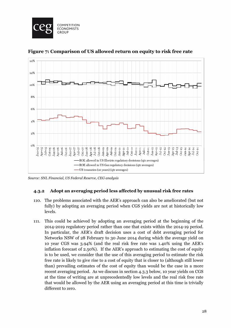
20. Over the 20 days to 19 December 2014, the risk free rate proxied by 10 year yields on CGS was 3.07%. Combined with an estimate for �� of 11.64%, this gives rise to an estimate of �� of 8.57%. Applying an equity beta of 0.82 results in a cost of equity of 10.10% during this period.

2.3 The historical average approach

21. The historical average approach is an internally consistent approach that can be applied if the MRP is to be determined as a stable estimate based primarily on a long term historical average. It requires that the risk free rate also be proxied by government bond yields sampled over a date range consistent with the measurement period for the MRP.

22. NERA’s update of the Brailsford et al data indicates that the average observed excess return on the market over 1883 to 2013 is slightly higher than the average over 1883 to 2011, at 6.56%.

4 CEG, WACC estimates: a report for NSW DNSPs, May 2014, p. 26

5 NERA, The market, size and value premiums, 2013.

6 Brailsford, T., J. Handley and K. Maheswaran, Re-examination of the historical equity risk premium in Australia, Accounting and Finance 48, 2008.

6

23. Over the commensurate period the average real bond yield was 2.21%. This is equivalent to a nominal bond yield of 4.77% when combined with expectations of inflation of 2.50%.

24. With an estimate of equity beta of 0.82, these estimates give rise to a total estimate of the cost of equity under this approach of 10.15%.

2.4 DGM to derive an MRP for the Sharpe CAPM

25. The DGM seeks to estimate the cost of equity implied by current stock prices given future expected dividend cash flows. If conducted on the stock market as a whole it can provide prevailing estimates of �� and ��.

26. We use an implementation of the DGM that aligns with the methodology applied by the AER. However, we prefer our own estimate of the long run growth rate of dividends per share of 3.75% in real terms. We also apply an uplift of 11.3% to dividends to account for the value of imputation credits, based on a value for theta of 0.35.

27. With these assumptions, over the Networks NSW cost of debt averaging period the average estimate of �� is 11.4% using the three-stage DGM and assuming that long run dividend growth is around 0.75% less than GDP growth.

28. Given contemporaneous yields on 10 year CGS of 3.94%, this implies a prevailing estimate for �� of 7.48% in that period. (This is slightly lower than the equivalent MRP estimated using the Wright method (7.70%)). With an estimate for equity beta of 0.82, this gives rise to a cost of equity of 10.07%.

29. Over the more recent 20 day period ending 19 December 2014, the average estimate of �� is 11.27% using the three-stage DGM and assuming that long run dividend growth is around 0.75% less than GDP growth. 10 year CGS yields in this period average 3.07%, implying a prevailing estimate for MRP of 8.20%.7 This is consistent with an estimate for the cost of equity of 9.79%.

30. SFG has also applied the DGM model,8 to the period 28 February 2014 to 30 June 2014. SFG’s DGM estimate of the MRP in this period is 7.48% exactly the same (to two decimal places) as our estimate. (SFG gives this estimate 50% weight and also gives weight to other estimates, including historical average excess returns to arrive at its final estimate of an MRP of 7.33%).

7 This is slightly lower than the equivalent MRP estimated using the Wright method of 8.57%.

8 SFG, The required return on equity: Initial review of the AER draft decisions, January 2015.

7

2.5 Black CAPM

31. In implementing the Black CAPM, our previous report noted that a review of the finance literature and recent empirical analysis performed by SFG suggests that:

�� − �� − � ��. � ��

= 0.50

32. This formula can be rearranged to be expressed as an estimate for the required return on a zero beta portfolio.

33. Over the period 28 February to 30 June 2014 our DGM estimate of �� is 11.42%%. Given yields on 10 year CGS of 3.94%, this suggests an estimate for �� of 7.68%.9 Using an equity beta of 0.82, this gives rise to an estimate for the cost of equity of 10.75%.

34. In the 20 day period ending 19 December 2014, our DGM estimate of �� is 11.27% and 10 year CGS yields are 3.07%. The estimate for �� from the equation above is 7.17%. The corresponding cost of equity is 10.53%.

35. SFG has also estimated a Black CAPM cost of equity over the period 28 February to 30 June 2014 and its estimate is 10.54%.10

2.6 Fama French model

36. SFG previously used the Fama French three factor model to estimate that the cost of equity under long term average market conditions was 11.5%. Using estimates of prevailing bond rates and �� reflecting prevailing DGM based estimates, we estimated a cost of equity of 10.9% in our May 2014 report. SFG’s updated estimate for the period 28 February to 30 June 2014 is 10.79%.11

2.7 Summary of estimates

37. The estimates discussed above are, for the most case, lower bound estimates of the cost of equity. This is because the methods that use an implementation of the Sharpe-Lintner CAPM formula have not been corrected for low-beta bias since we have applied an econometrically estimated beta of 0.82. Only the Black CAPM and FFM estimates are free from this bias.

9 Based on the work of Professor Grundy, and as set out in our May 2014 report, we estimate the zero beta

premium as half of the MRP(0.5*7.48%=3.74%). Adding this to the risk free rate (3.94%) gives a zero beta return of 7.68%.



8

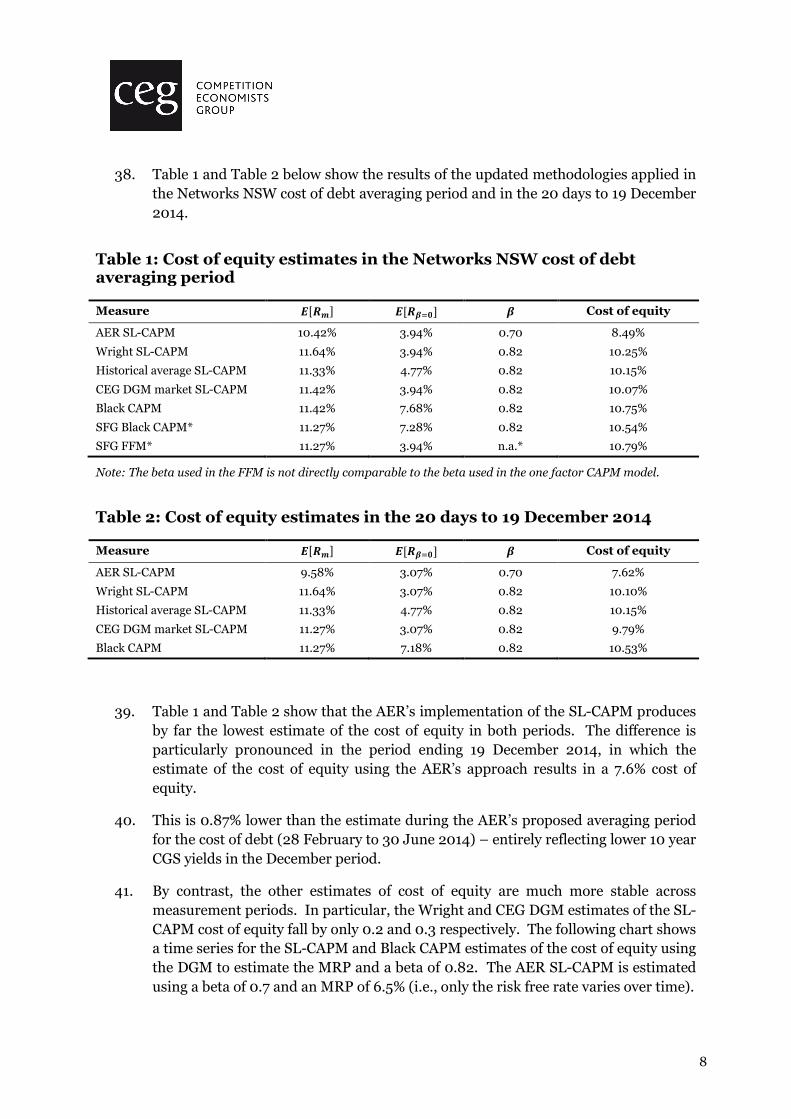
38. Table 1 and Table 2 below show the results of the updated methodologies applied in the Networks NSW cost of debt averaging period and in the 20 days to 19 December 2014.

Table 1: Cost of equity estimates in the Networks NSW cost of debt averaging period

Measure �� Cost of equity

AER SL-CAPM 10.42% 3.94% 0.70 8.49%

Wright SL-CAPM 11.64% 3.94% 0.82 10.25%

Historical average SL-CAPM 11.33% 4.77% 0.82 10.15%

CEG DGM market SL-CAPM 11.42% 3.94% 0.82 10.07%

Black CAPM 11.42% 7.68% 0.82 10.75%

SFG Black CAPM* 11.27% 7.28% 0.82 10.54%

SFG FFM* 11.27% 3.94% n.a.* 10.79%

Note: The beta used in the FFM is not directly comparable to the beta used in the one factor CAPM model.

Table 2: Cost of equity estimates in the 20 days to 19 December 2014

Measure �� Cost of equity

AER SL-CAPM 9.58% 3.07% 0.70 7.62%

Wright SL-CAPM 11.64% 3.07% 0.82 10.10%

Historical average SL-CAPM 11.33% 4.77% 0.82 10.15%

CEG DGM market SL-CAPM 11.27% 3.07% 0.82 9.79%

Black CAPM 11.27% 7.18% 0.82 10.53%

39. Table 1 and Table 2 show that the AER’s implementation of the SL-CAPM produces by far the lowest estimate of the cost of equity in both periods. The difference is particularly pronounced in the period ending 19 December 2014, in which the estimate of the cost of equity using the AER’s approach results in a 7.6% cost of equity.

40. This is 0.87% lower than the estimate during the AER’s proposed averaging period for the cost of debt (28 February to 30 June 2014) – entirely reflecting lower 10 year CGS yields in the December period.

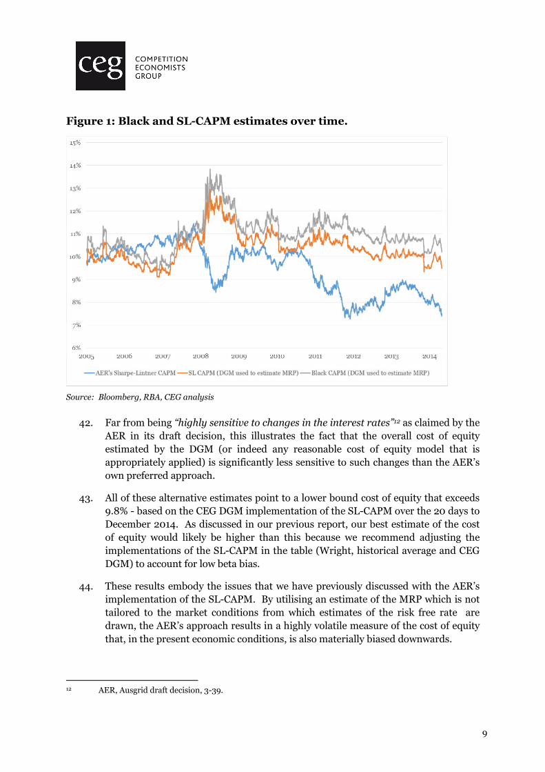
41. By contrast, the other estimates of cost of equity are much more stable across measurement periods. In particular, the Wright and CEG DGM estimates of the SL-CAPM cost of equity fall by only 0.2 and 0.3 respectively. The following chart shows a time series for the SL-CAPM and Black CAPM estimates of the cost of equity using the DGM to estimate the MRP and a beta of 0.82. The AER SL-CAPM is estimated using a beta of 0.7 and an MRP of 6.5% (i.e., only the risk free rate varies over time).

9

Figure 1: Black and SL-CAPM estimates over time.

Source: Bloomberg, RBA, CEG analysis

42. Far from being “highly sensitive to changes in the interest rates”12 as claimed by the AER in its draft decision, this illustrates the fact that the overall cost of equity estimated by the DGM (or indeed any reasonable cost of equity model that is appropriately applied) is significantly less sensitive to such changes than the AER’s own preferred approach.

43. All of these alternative estimates point to a lower bound cost of equity that exceeds 9.8% - based on the CEG DGM implementation of the SL-CAPM over the 20 days to December 2014. As discussed in our previous report, our best estimate of the cost of equity would likely be higher than this because we recommend adjusting the implementations of the SL-CAPM in the table (Wright, historical average and CEG DGM) to account for low beta bias.

44. These results embody the issues that we have previously discussed with the AER’s implementation of the SL-CAPM. By utilising an estimate of the MRP which is not tailored to the market conditions from which estimates of the risk free rate are drawn, the AER’s approach results in a highly volatile measure of the cost of equity that, in the present economic conditions, is also materially biased downwards.

12 AER, Ausgrid draft decision, 3-39.

10

3 Dividend growth model estimates 45. This section sets out updated estimates of the DGM applied to the Australian stock

market to those presented in our previous report for the Networks NSW businesses.13

46. We also adapt the same methodology to apply it to the four currently traded utility stocks used by the AER in its equity beta sample – specifically APA Group, AusNet Services, DUET, and Spark Infrastructure.

3.1 Dividend growth model for the market

47. In our previous report we estimated a DGM for the market for the 20 days ending 13 May 2014.14 We undertook this analysis using the methodology described by the AER in Appendix E.2 of its December 2013 Rate of Return Guideline.

48. In this section we update this analysis up to 19 December 2014. We also apply the same methodology over a time series using input data from Bloomberg back to 25 August 2005. This is the earliest date from which we were able to source a continuous time series of dividend forecasts for the Australian stock market index.

49. We summarise the results of our updated DGM, both over the Network NSW cost of debt averaging period and also over the most recent 20 day period ending 19 December 2014.

3.1.1 Updated CEG results

50. Our updated application of the DGM continues to use the same implementation of the AER’s approach that we previously described. The key features of this approach are:

� daily forecasts of dividends for the ASX 200 index are sourced from Bloomberg for the current financial year, the next financial year and the following financial year. Daily prices for the ASX 200 index are also sourced from Bloomberg;

� for dividend forecasts of the current financial year, the dividend cashflow is assumed to occur midway between the forecast date and the end of the financial year for a pro-rata amount commensurate with the proportion of the year remaining. Future dividend cash-flows are assumed to occur midway through the financial year;


14 CEG, WACC estimates: a report for NSW DNSPs, May 2014, pp. 20-26

11

� two-stage and three-stage models are developed. The two-stage model assumes that the long run dividend growth rate occurs immediately after the forecast horizon. The three-stage model assumes an 8 year transition from the growth rate in dividends implied by the last two years of dividend forecasts to the long run growth rate;

� in the final year a terminal value is calculated assuming constant growth of dividends at the long run dividend growth rate from that year onwards; and

� we uplift the dividend forecasts to account for the value of imputation credits to shareholders. Following the AER’s approach, we apply an uplift factor of 1.1125, calculated as:

1 + "#�

1 − �

where:

" is the utilisation rate of imputation credits which we assume to be 35%;

# is the proportion of dividends issued with imputation credits. We use the AER’s proposed parameter value of 75%; and

� is the corporate tax rate of 30%.

51. The single discount rate that reconciles the present value of the stream of dividends calculated under the assumptions above with the value of the ASX 200 index is an estimate of the implied market cost of equity, or ��, on that day. The MRP implied from that discount rate can be calculated by subtracting the risk free rate proxy, the 10 year yields on CGS, from this estimate.

52. The key parameter that populates this model is an estimate for the long run growth rate for dividend per share forecasts. In our previous report we stated our preference for an estimate based on the long run growth rate of real GDP less 0.5% to 1.0%. Our view was that the best estimate for GDP growth over the long term was likely to be 3.75%.15 However, consistent with our previous report we consider sensitivities to this estimate by modelling a long run growth rate for dividends that is up to 1.5% lower than this estimate.

53. Table 3 below shows the result of this DGM applied to both the Networks NSW cost of debt averaging period. Table 4 beneath it shows the results of the DGM estimated over the 20 day period ending 19 December 2014.

15 CEG, WACC estimates: a report for NSW DNSPs, May 2014, pp. 22-25

12

Table 3: CEG’s estimates of MRP over the Networks NSW cost of debt averaging period

�� $�%�

Two stage model (no transition)

Three stage model (transition over 8

years)



years)

d=0.0% 11.93 12.03 7.99 8.09

d=0.5% 11.46 11.62 7.51 7.68

d=1.0% 10.97 11.22 7.03 7.28

d=1.5% 10.49 10.82 6.54 6.88

Source: Bloomberg data, CEG analysis

Table 4: CEG’s estimates of MRP over the 20 days ending 19 December 2014

�� $�%�



years)



years)

d=0.0% 11.94 11.87 8.86 8.79

d=0.5% 11.47 11.47 8.39 8.39

d=1.0% 11.00 11.07 7.91 7.99

d=1.5% 10.52 10.68 7.44 7.60


54. Table 3 and Table 4 illustrate that the results of the DGM analysis are stable. Estimates of �� are almost unchanged between the Networks NSW cost of debt averaging period and the 20 days to 19 December 2014.

55. This is in stark contrast to the estimate of �� which results from the simple addition of the AER’s fixed MRP to the prevailing CGS yields. Under the AER’s methodology, the entire 0.9% fall in CGS yields is assumed to be associated with an commensurate fall in investors’ required return on equities.

56. However, if this were actually the case then it must be that share market prices for equity would need to have increased by a corresponding proportion (or dividend forecasts to have fallen). That is, if investors’ discount rates fell then, holding dividend forecasts constant, then the price investors are prepared to pay for equities must rise. The DGM provides a test of the AER’s simple model.

57. The results presented above demonstrate that equity prices relative to dividend forecasts did not move in a manner consistent with that required if the AER’s simple model were correct. The market value of shares relative to dividend forecasts has

13

remained roughly the same – implying investors’ required discount rate (��) has remained roughly the same.

58. The AER’s proposed cost of equity methodology results in the estimated cost of equity being highly sensitive to movements in the risk free rate, moving on a one-for-one basis with it. This relationship between the cost of equity and the risk free rate is much more sensitive than is justified by the evidence from the consistent application of the DGM model over time. The relatively stable value for �� between the Networks NSW cost of debt averaging period and the 20 days to 19 December 2014 means that the fall in the risk free rate proxy from 3.94% to 3.07% between these periods has resulted in largely offsetting increases in the prevailing estimates of MRP.16

59. The AER’s proposed MRP estimate of 6.5% is not within the range set out in Table 4 and is not consistent with the central estimates of 8.4%/7.9% associated with d=0.5/1.0. In our opinion, the appropriate period over which to use DGM estimates is over a period consistent within which the risk free rate is estimated. This is to ensure consistency between the risk free rate assumptions in the SL-CAPM formula below:

�& = �' + ()*�� − �'+

60. If we do not estimate the DGM in the same period as the risk free rate assumption, then we fall into the same error as the AER in its estimation of an MRP inconsistently with its value of the risk free rate.

61. Consistent with these MRP estimates, we have estimated the risk free rate over the same 20 days to 19 December 2014. We estimate this as the annualised yield on Commonwealth Government securities, interpolated to 10 years. Our estimate for this value is 3.07%.

3.1.2 Time series of DGM results

62. Figure 2 below shows the results of the three stage DGM applied each working day between 25 August 2005 and 19 December 2014. This provides a long period of history over which to assess the results of the DGM methodology.

63. Figure 2 shows that the estimate of MRP has been elevated compared to since mid-2011. That is, the current elevated levels are not a short term phenomenon.

16 These estimates are derived as annualised interpolated 10 year yields on CGS. The CGS yield data is

reported by the RBA.

14

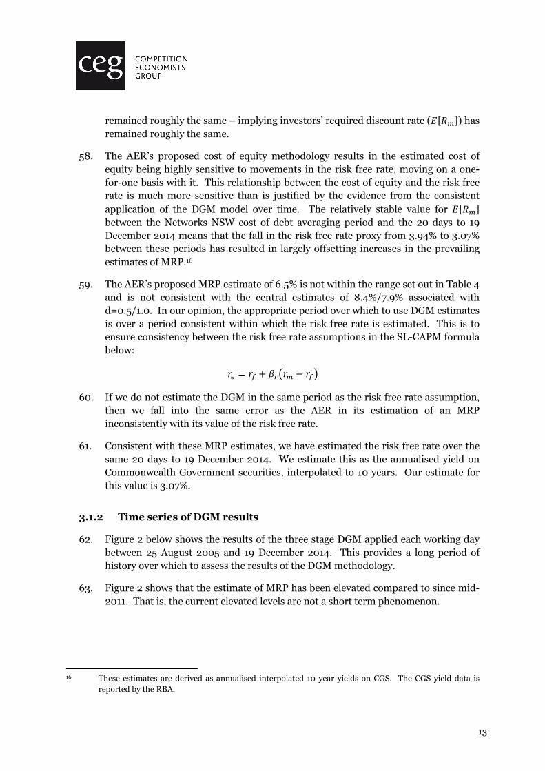
Figure 2: Time series of MRP and risk free rate, three stage DGM with 8 year transition, d=0.75%


64. This figure also shows that despite recent oscillation, the market return on equity implied by the DGM remains in excess of 11%, averaging 11.4% over the 20 days to 19 December 2014. By contrast, over this time period the AER’s preferred parameter estimates for the risk free rate (3.1% in this period) and MRP (constant at 6.5%) imply an expected market return of 9.6%. This is nearly 2% less than the market return indicated in Figure 2. The difference would be even higher if a higher value was placed on imputation credits as is assumed by the AER.17

65. Irrespective of the level of the estimated MRP, which depends on the assumed value of d, the pattern in the above chart is clear. The MRP generally moves in the opposite direction to the risk free rate – with the effect that the market return on equity is more stable than if the MRP were assumed to be constant.

66. Figure 2 demonstrates the key issues with the AER’s proposed methodology for estimating the cost of equity. Namely that:

17 The AER draft decision adopts a value of 0.6 for theta while we adopt a value of 0.35.

15

� the expected market return on equity is much more stable than the risk free rate and does not move on a one-for-one basis with the risk free rate, as the AER’s methodology assumes. While it is not constant over time, the market return on equity has been relatively stable over the past 48 months; and

� as a result there is an inverse relationship between the MRP and the risk free rate.

67. This result is shown using a three stage DGM model that relies on analysts’ forecasts of dividends for the next two years and then trends dividends to long run growth levels over the next 8 years – which is what is shown in Figure 2. However, it is equally true of a one stage dividend growth model – which can be used to generate estimates over a longer horizon – from before Bloomberg publishes analyst forecasts of dividends.

68. We have used the dividend yield series published by the RBA to perform a DGM analysis using the method set out by AMP Capital Investors – which is effectively a one stage DGM that simply assumes that dividends grow at their long run level immediately. Prior to the GFC, this methodology was relied on by the AER in support of a position that the then MRP of 6.0% was generous.18

A more recent estimate is from AMP Capital Investors (2006), who base

the growth rate on the expected long-run GDP growth rate, similar to

Davis (1998). AMP Capital Investors (2006) estimate the forward looking

Australian MRP for the next 5-10 years to be ‘around 3.5 per cent’

(specifically 3.8 per cent), 1.9 per cent for the US and 2.4 per cent for the

‘world’. AMP Capital Investors (2006) considers an extra 1 to 1.5 per cent

could be added for imputation credits resulting in a ‘grossed-up’

Australian MRP of around 4.5 to 5.0 per cent.

69. The AMP methodology involves approximating a cost of equity by adding the long term average real growth in GDP (as a proxy for long term average nominal growth in dividends) to the prevailing dividend yield for the market as a whole. This gives a ‘cash’ cost of equity. To convert this into a cost of equity including the value of imputation credits, the cost of equity needs to be scaled up by the relevant factor.

70. Notwithstanding AMP’s use of GDP growth, Figure 3 below we have used 3.0% per annum as the long run growth path for real dividends (consistent with the 3.75% GDP growth assumption described earlier less a “d” of 0.75%). We have used a scaling factor of 1.1125 to capture the value of imputation credits.19 These

18 AER, Explanatory Statement, Electricity transmission and distribution network service providers

Review of the weighted average cost of capital (WACC) parameters, December 2008, p. 173

19 This is based on the assumption of a corporate tax rate of 30%; and, that the value of imputation credits distributed (theta) is 35% of their face value, consistent with Australian Competition Tribunal precedent; and that the proportion of dividends that are franked is 75% (consistent with Brailsford, T., J. Handley

16

assumptions are important for the level but not for the variation in the cost of equity estimate.

71. In Figure 3 below we compare the real market cost of equity (��) estimated in this manner with the real yield on CPI indexed CGS. We also show the implied MRP – which is just the difference between these two series. (We use the real series in this chart because our time series extends back into high expected inflation periods – making comparisons different if the series are in nominal terms.)

72. The estimate of E[Rm], being the sum of the CGS and MRP time series is much more stable than either of these two time series.

Figure 3: AMP method estimate of real E[Rm] and E[MRP] relative to 10 year indexed CGS yields

Source: RBA and CEG analysis.

73. This chart illustrates the same inverse relationship between the MRP series and the risk free rate series as in Figure 2 but over a much longer time horizon. When one is high then the other us low and vice versa. This is a result of the stability in the estimated E[Rm] series which, itself, reflects stability in the dividend yield series

and K. Maheswaran, Re-examination of the historical equity risk premium in Australia, Accounting and Finance 48, 2008, page 85). The value of 1.1125 is calculated as 1+.30*.35*.75/(1-.3).

17

(noting that this is a one period DGM model with a constant dividend growth forecast).

74. Figure 2 and Figure 3 demonstrate that, whether one adopts a one stage or a three stage DGM model, the same basic result exists. Namely, the cost of equity does not vary with the risk free rate in the way the AER methodology presumes. Historically low risk free rates do not imply historically low required return on equity.

75. The sentiments expressed in the below quote by Professor Damodaran capture precisely this point.20

It is true that riskfree rates are low but they are not the only numbers at

unusual levels. Equity risk premiums and default spreads are at historical

highs and the worry about global economic growth is deeper than at time

in recent history. When we use low riskfree rates in valuation, we

have to accompany them with much higher risk premiums than

we would have used a few months ago, lower real growth and

lower expected inflation. The net effect is that intrinsic values are

lower now than they were a few months ago.

What gets analysts into trouble is inconsistency. If we use today's

riskfree rates and stick with risk premiums that we used to use in the past

and growth rates and inflation rates that are also from the past, we will

over value companies. The culprit is not the low riskfree rates but

internal inconsistency.

My advice is that you stay with today's riskfree rates but update the other

numbers you use in valuation to reflect the environment we face right

now. If you insist on replacing today's riskfree rate with your normalized

number, you should then adjust all your other numbers to be consistent -

not easy to do, in my view. [Emphasis added]

3.1.3 Cross check with AER results

76. We have attempted to cross check the results of our DGM with the AER’s. Since we are attempting to apply the AER’s model, we would expect that the results of our methodologies should be aligned when applied with the same inputs.

77. However, during the period modelled by the AER in its draft decision we find that our estimates of MRP are approximately 0.4% lower than those reported by the AER. This is demonstrated by a comparison of the AER’s estimates in Table 5 below against those that we generate using apparently identical assumptions in Table 6.

20 Aswath Damodaran, Professor of Finance at Stern School of Finance, NYU, “Musing on Markets”, 2

February 2009, http://aswathdamodaran.blogspot.com.au/2009/02/low-riskfree-rates.html.

18

Table 5: AER’s estimates of MRP (two months ending 30 September 2014)

Growth rate Two stage model Three stage model

4.0 6.6 7.0

4.6 7.2 7.4

5.1 7.7 7.8

Source: AER

Table 6: CEG’s estimates of MRP (two months ending 30 September 2014)

�� $�%�



years)



years)

4.0 10.0 10.1 6.5 6.6

4.6 10.6 10.6 7.0 7.0

5.1 11.0 11.0 7.5 7.4


78. We are unable to explain this difference between these results, since the AER provides clear explanations of:

� its uplift assumptions (p. 3-206); and

� its cash-flow timing assumptions (p. 3-213).

79. However, there is less clarity about which series the AER uses within Bloomberg to source analyst forecasts of dividends, so it is possible that discrepancies could originate in relation to these assumptions. It is also possible that some of the AER’s input assumptions have been reported on a rounded basis but used on an unrounded basis, which could also contribute to differences in the results. However, this would be unlikely to explain the extent of the variances between the estimates.

80. We note that we can explain about half the difference between these estimates if we apply an estimate of theta of 0.7 (as the AER assumes in its Rate of Return Guideline) rather than 0.6 that the AER proposes in its draft decision. However, again this does not reconcile the values.

81. Given the divergences between our estimates over the months to the end of September 2014, we expect that it is likely that our estimates described above are also likely to underestimate the results that the AER would obtain using the same parameters.

19

3.2 Dividend growth model for utilities

82. Just as is the case for the market DGM, DGM estimates of the return on equity for individual regulated utilities equate the present value of forecast future dividends with the current price of the equity. The discount rate that makes these equal is an estimate of the return on equity expected by investors in these stocks.

83. In this section we apply the DGM methodology to APA Group, AusNet Services, DUET and Spark Infrastructure. This analysis differs from the DGM on the market since we can apply firm-specific dividend yields and forecasts, including the specific timing of expected cash flows.

3.2.1 Methodology

84. We have followed the AER’s DGM methodology21, adapted to apply to specific equities as opposed to a market portfolio. Differences to the AER’s model are described in this section.

85. We have applied the same dividend growth rates as for the market DGM as well as reporting a zero real growth in dividends as a conservative estimate. Assuming the expected inflation is 2.5% and the expected long-run real growth in dividends is zero, then the expected long-run nominal growth in dividends is 2.5%.

86. For the market DGM we apply market wide parameters on the value of franking credits. For individual utilities stocks we have assumed benchmark parameters as applied in the PTRM – i.e. theta = 0.35 and 100% franking of dividends.

87. Bloomberg publishes consensus forecasts for dividends issued by firms between one and five years into the future. We use all of this data, transitioning to the long-run growth rate either from the first year after the final forecast (in the two-stage model) or from the tenth year onwards (in the three-stage model).

88. When we are forecasting dividend cash flows from a single firm, as opposed to an index composed on 200 firms, we can generate more precise estimates about when these dividends will be paid. Specifically, in estimating the timing of future cash flows we have regard to the payment dates of recent dividends. We consider ex-dividend dates associated with the payments to determine whether to account for future dividend payments in the DGM.

3.2.2 Comparator set

89. The AER identified a set of reasonable comparators to the benchmark efficient entity – ASX listed firms that provide regulated electricity and/or gas network

21 Set out in appendix E.2 of the December 2013 Rate of Return Guideline

20

services operating within Australia.22 We have focussed on the four firms that are still listed on the stock market.

3.2.3 Results

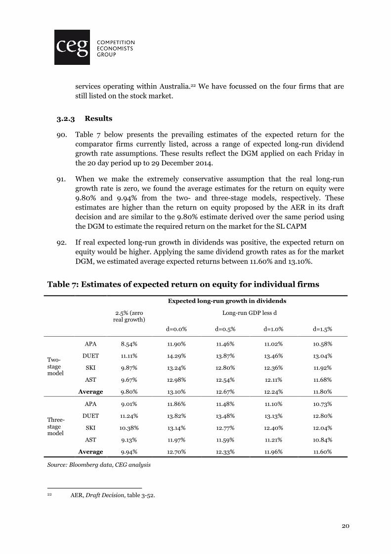
90. Table 7 below presents the prevailing estimates of the expected return for the comparator firms currently listed, across a range of expected long-run dividend growth rate assumptions. These results reflect the DGM applied on each Friday in the 20 day period up to 29 December 2014.

91. When we make the extremely conservative assumption that the real long-run growth rate is zero, we found the average estimates for the return on equity were 9.80% and 9.94% from the two- and three-stage models, respectively. These estimates are higher than the return on equity proposed by the AER in its draft decision and are similar to the 9.80% estimate derived over the same period using the DGM to estimate the required return on the market for the SL CAPM

92. If real expected long-run growth in dividends was positive, the expected return on equity would be higher. Applying the same dividend growth rates as for the market DGM, we estimated average expected returns between 11.60% and 13.10%.

Table 7: Estimates of expected return on equity for individual firms

Expected long-run growth in dividends

2.5% (zero real growth)

Long-run GDP less d

d=0.0% d=0.5% d=1.0% d=1.5%

Two-stage model

APA 8.54% 11.90% 11.46% 11.02% 10.58%

DUET 11.11% 14.29% 13.87% 13.46% 13.04%

SKI 9.87% 13.24% 12.80% 12.36% 11.92%

AST 9.67% 12.98% 12.54% 12.11% 11.68%

Average 9.80% 13.10% 12.67% 12.24% 11.80%

Three-stage model

APA 9.01% 11.86% 11.48% 11.10% 10.73%

DUET 11.24% 13.82% 13.48% 13.13% 12.80%

SKI 10.38% 13.14% 12.77% 12.40% 12.04%

AST 9.13% 11.97% 11.59% 11.21% 10.84%

Average 9.94% 12.70% 12.33% 11.96% 11.60%


22 AER, Draft Decision, table 3-52.

21

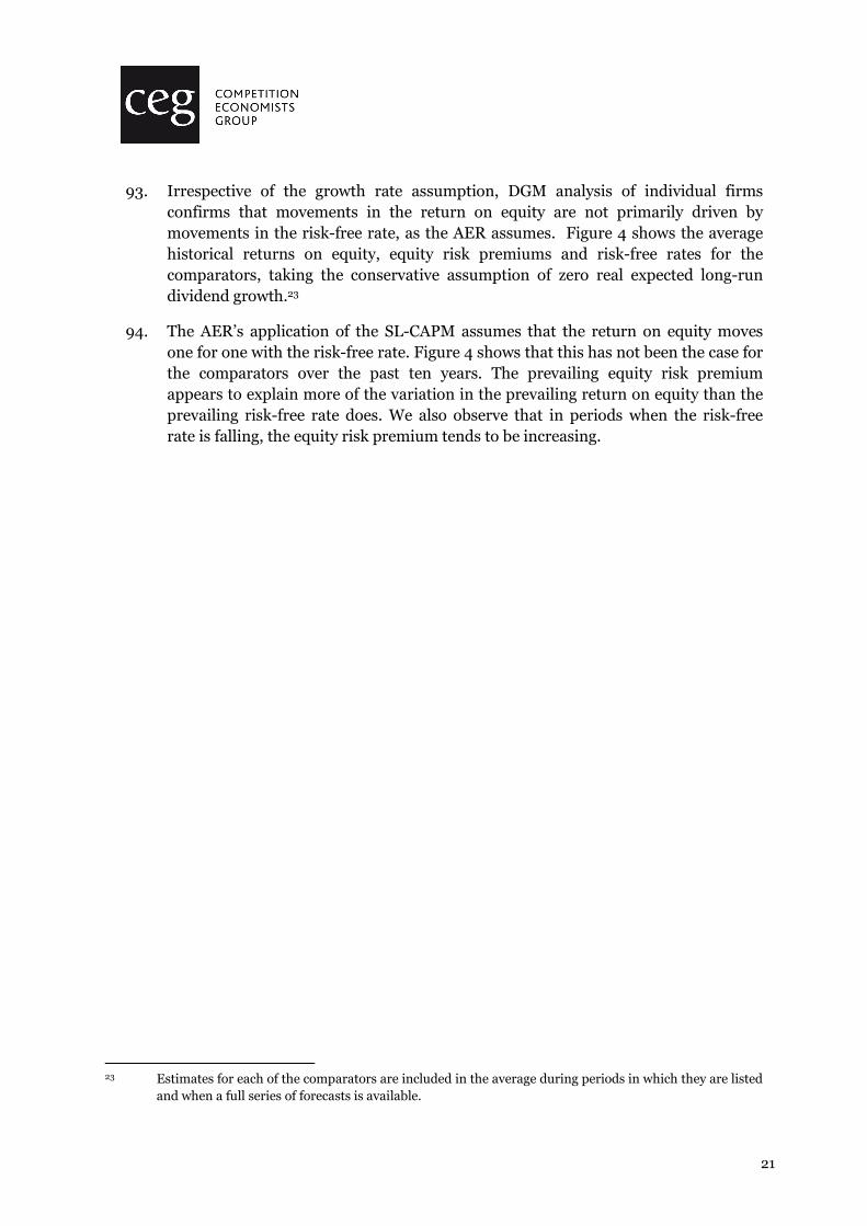
93. Irrespective of the growth rate assumption, DGM analysis of individual firms confirms that movements in the return on equity are not primarily driven by movements in the risk-free rate, as the AER assumes. Figure 4 shows the average historical returns on equity, equity risk premiums and risk-free rates for the comparators, taking the conservative assumption of zero real expected long-run dividend growth.23

94. The AER’s application of the SL-CAPM assumes that the return on equity moves one for one with the risk-free rate. Figure 4 shows that this has not been the case for the comparators over the past ten years. The prevailing equity risk premium appears to explain more of the variation in the prevailing return on equity than the prevailing risk-free rate does. We also observe that in periods when the risk-free rate is falling, the equity risk premium tends to be increasing.

23 Estimates for each of the comparators are included in the average during periods in which they are listed

and when a full series of forecasts is available.

22

Figure 4 Time series return on equity, ERP and risk free rate, three-stage model24


24 This assumes zero real expected long-run dividend growth. Hastings Diversified Utilities Fund was

included in the average from 11 November 2005 to 23 November 2012, at which point its trading was suspended. HDF’s decreasing return on equity from December 2011 may have been affected by APA’s offer to acquire HDF. During this period HDF’s implied cost of equity was consistent with or below that of other firms. Ausnet was included from 27 January 2006 onwards, initially as SP Ausnet. Envestra was included until 12 September 2014 when its trading was suspended. Envestra’s return on equity from July 2013 onwards may have been affected by expectations of an acquisition however our estimates for Envestra’s return on equity during this period are consistent with those of other firms.

23

4 Historically unprecedented CGS yields

4.1 Historical overview

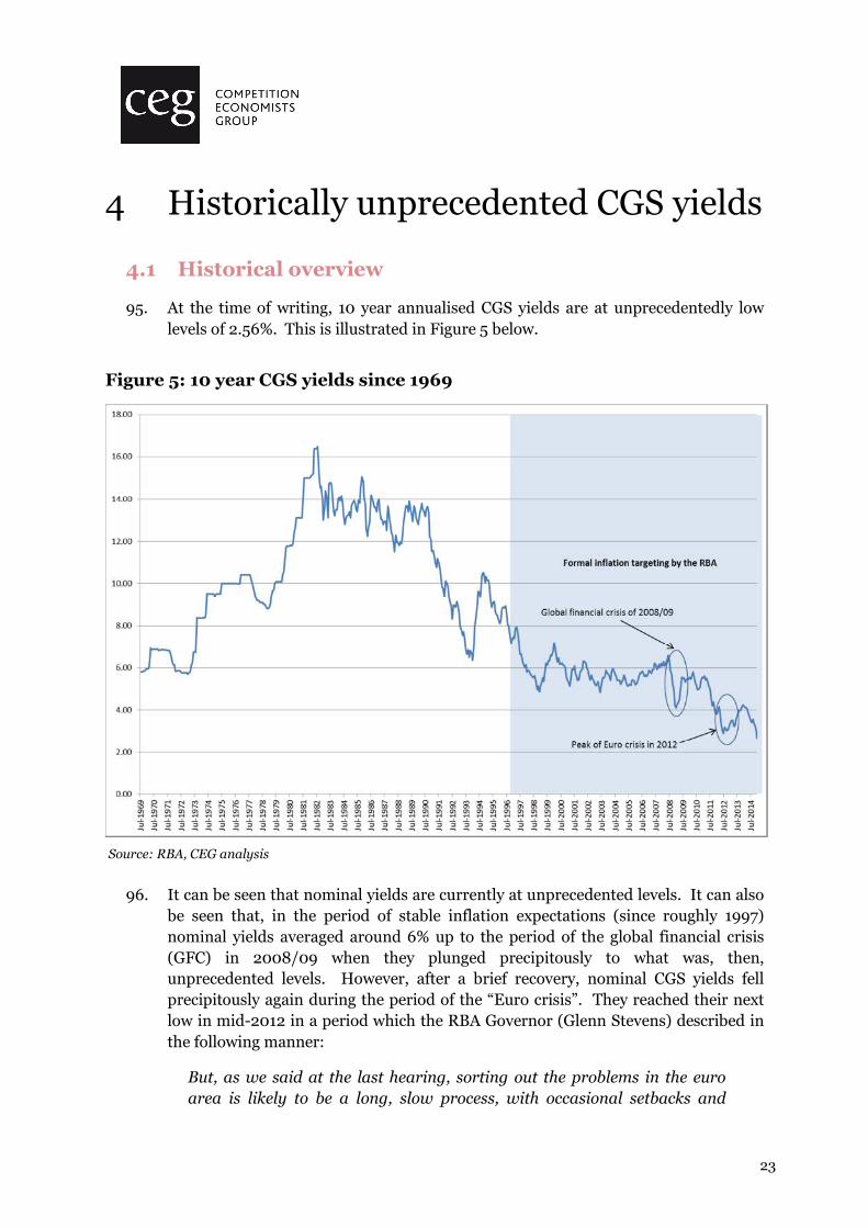
95. At the time of writing, 10 year annualised CGS yields are at unprecedentedly low levels of 2.56%. This is illustrated in Figure 5 below.

Figure 5: 10 year CGS yields since 1969

Source: RBA, CEG analysis

96. It can be seen that nominal yields are currently at unprecedented levels. It can also be seen that, in the period of stable inflation expectations (since roughly 1997) nominal yields averaged around 6% up to the period of the global financial crisis (GFC) in 2008/09 when they plunged precipitously to what was, then, unprecedented levels. However, after a brief recovery, nominal CGS yields fell precipitously again during the period of the “Euro crisis”. They reached their next low in mid-2012 in a period which the RBA Governor (Glenn Stevens) described in the following manner:

But, as we said at the last hearing, sorting out the problems in the euro

area is likely to be a long, slow process, with occasional setbacks and

24

periodic bouts of heightened anxiety. We saw one such bout of

anxiety in the middle of this year, when financial markets displayed

increasing nervousness about the finances of the Spanish banking system

and the Spanish sovereign. The general increase in risk aversion saw

yields on bonds issued by some European sovereigns spike higher, while

those for Germany, the UK and the US declined to record lows. This

‘flight to safety’ also saw market yields on Australian government debt

decline to the lowest levels since Federation. [Emphasis added]

97. It is clear from these remarks that Governor Stevens did not view the then historic lows in CGS as being associated with a similarly low market cost of equity. On the contrary, low CGS yields were directly associated by Stevens with raised risk aversion and a ‘flight to safety’. That is, the causal mechanism went from heightened perceived risk of equities (and other risky assets) causing a ‘flight to safety’ and driving down risk free rates.

98. Since then, CGS yields recovered modestly but have since fallen over 2014 to be below the previous “post Federation” lows referred to by Governor Stevens.

4.2 What is driving low CGS yields? And is it also driving

low equity yields?

99. Since the GFC, CGS yields have, as evidenced in Figure 5, been depressed relative to their pre-crisis levels – no matter what pre crisis time period is examined. The important issue for estimating the cost of equity is to answer two questions:

� What is driving low CGS yields in post GFC (in general or in any specific averaging period)? and

� Can the same factors be expected to drive similarly low returns on risky equities?

100. If the answer to the second question is no, then this underscores the need to ensure that the expected return on the equity market (and therefore the MRP) estimate is tailored to the specific market circumstances from which the risk free rate estimate (based on CGS yields) is taken.

101. Governor Stevens has already clearly set out his belief that the previous historic lows in CGS yields were driven by factors that, if anything, could be expected to raise the cost of equity rather than lower it (i.e., heightened risk aversion – a side effect of which was a flight to safety which lowered yields on safe assets).

102. More generally, both the RBA and the IMF have observed a number of persistent factors that would be expected to lower CGS yields after the GFC but which cannot be expected to lower the required returns on risky assets. We survey these in more detail in Appendix A. In summary:

25

� shrinking supply of AAA rated Sovereign debt globally (IMF,25 RBA Assistant Governor Debelle,26 Australian Office of Financial Management27) and shrinking supply of substitutes in the form of safe private sector debt (IMF28);

� heightened risk aversion and increased levels of perceived risk (RBA Governor Stevens as described above, RBA Assistant Governor Debelle,29 Australian Office of Financial Management30); and

� heightened demand for liquid assets post GFC - including due to changes to banking regulations (IMF, 31 RBA, 32 33 34, APRA35).

103. As an example of the last point, RBA Assistant Governor Debelle has, in December 2014, expressed the view that the implementation of Basel III liquidity

25 IMF, Global Financial Stability Report, April 2012, Chapter 3, Safe assets: Financial System

Cornerstone. Available at http://www.imf.org/external/pubs/ft/gfsr/2012/01/pdf/c3.pdf. See See IMF summary at: http://www.imf.org/external/pubs/ft/survey/so/2012/POL041112A.htm.

26 RBA, Letter regarding the Commonwealth Government Securities Market, Guy Debelle, Assistant Governor, Financial Markets, Reserve Bank of Australia, 16th July 2012. See paragraph 2 on page 1 first sentence.

27 Australian Government, The Treasury, Letter to Joe Dimasi, ACCC, regarding the Commonwealth

Government Securities Market, 18th July 2012. See paragraph 3 on page 1. Also, paragraph 2 under the first question answered on page 2.

28 IMF, Global Financial Stability Report, April 2012, Chapter 3, Safe assets: Financial System Cornerstone, p. 108.

29 RBA, Letter regarding the Commonwealth Government Securities Market, Guy Debelle, Assistant Governor, Financial Markets, Reserve Bank of Australia, 16th July 2012. See paragraph 2 on page 1.

30 Australian Government, The Treasury, Letter to Joe Dimasi, ACCC, regarding the Commonwealth

Government Securities Market, 18th July 2012. See paragraphs 3 and 4 under the first question answered on page 2. Also final paragraph under the first question answered on page 2.

31 IMF, Global Financial Stability Report, April 2012, Chapter 3, Safe assets: Financial System Cornerstone. Box 3.4 on page 100 “Impact of the Basel III Liquidity Coverage Ration on the Demand for Safe Assets”.

32 Guy Debelle, RBA Assistant Governor (Financial Markets), Speech to the APRA Basel III Implementation Workshop 2011 Sydney - 23 November 2011.

33 Lancaster and Dowling, The Australian Semi-government Bond Market, RBA bulletin, September Quarter 2011.

34 Guy Debelle, Assistant Governor (Financial Markets), Speech at the 27th Australasian Finance and Banking Conference, Sydney - 16 December 2014.

35 APRA’s Basel III Implementation rationale and impacts, Charles Littrell, Exec. GM, Policy, Research and Statistics, APRA, APRA Finsia Workshop, Sydney, 23 November 2011.

26

requirements are depressing CGS yields relative to the levels that they would otherwise be:36

I have talked before about some of the impact on pricing in various

markets of the new liquidity regime. We have attempted to limit the

impact on the price of CGS and semis, but necessarily, because

the banks are holding more of these securities than previously

(Graph 1), the price is higher (and the yield lower) than would

otherwise be the case. [Emphasis added.]

104. This evidence is discussed in more detail in Appendix A. However, none of these factors can reasonably be described as also causing the yield on risky assets to fall. Indeed, the yield on the Australian equity market most certainly has not fallen post GFC. This is illustrated in Figure 6 below.

Figure 6: Dividend yields on the Australian equity market vs yields on 10 year inflation indexed CGS

Source: Reserve Bank of Australia, CEG analysis

36 Guy Debelle, Assistant Governor (Financial Markets), Speech at the 27th Australasian Finance and

Banking Conference, Sydney - 16 December 2014.

27

105. This chart shows that, far from the dividend yield on Australian equities falling as real CGS yields fell post GFC,37 dividend yields have actually risen relative to pre-GFC levels (i.e., pre 2008). The most recent observation of 4.6% in December 2014 is higher than any observed dividend yields from 1993 up to the onset of the GFC in 2008. Indeed, it is at its highest point outside the worst of the GFC and the worst of the Euro zone debt crisis. This is despite CGS yields being at their lowest point at this time. Far from low CGS yields being associated with required return on equity the opposite appears to be the case – implying that the MRP measured relative to CGS has risen by a more than offsetting amount than the fall in CGS.

106. This is consistent with the sentiments of RBA Assistant Governor Guy Debelle’s letter to the AER where he reflects on a widening of risk premiums relative to CGS and states: 38

“This widening indeed confirms the market's assessment of the risk-free

nature of CGS and reflects a general increase in risk premia on other assets.”

4.3 Implications

4.3.1 Adopt a consistent approach to estimating the MRP and risk free rate

107. At the most fundamental level, it is not critical to agree on the reasons why nominal CGS yields are at their lowest ever levels. This fact does not mean that the CAPM or other models cannot be applied. Rather, for the reason set out below, it means that it is critical to estimate the MRP in a manner, and over a period, that is consistent with the risk free rate being estimated.

108. As set out in section 3.1 (and particularly section 3.1.2) the expected return on the market less the risk free rate (i.e., the expected MRP) varies significantly across time periods and tends to be inversely related to the risk free rate. A simplistic approach of adding a more or less fixed MRP (based mostly on historical average excess returns) will underestimate the MRP in current market conditions.

109. In this respect, we note that there are many regulators that do not implement the AER’s approach to estimating the cost of equity. In the United States, it is commonplace to use techniques such as the DGM to determine allowed cost of equity. The methodologies applied by United States regulators result in a cost of equity that in general does not vary one-for-one with the proxies for the risk free rate, as we show in Figure 7 below.

37 Or even prior to the GFC.

38 RBA, Letter regarding the Commonwealth Government Securities Market, Guy Debelle, Assistant Governor, Financial Markets, Reserve Bank of Australia, 16th July 2012.

28

Figure 7: Comparison of US allowed return on equity to risk free rate

Source: SNL Financial, US Federal Reserve, CEG analysis

4.3.2 Adopt an averaging period less affected by unusual risk free rates

110. The problems associated with the AER’s approach can also be ameliorated (but not fully) by adopting an averaging period when CGS yields are not at historically low levels.

111. This could be achieved by adopting an averaging period at the beginning of the 2014-2019 regulatory period rather than one that exists within the 2014-19 period. In particular, the AER’s draft decision uses a cost of debt averaging period for Networks NSW of 28 February to 30 June 2014 during which the average yield on 10 year CGS was 3.94% (and the real risk free rate was 1.40% using the AER’s inflation forecast of 2.50%). If the AER’s approach to estimating the cost of equity is to be used, we consider that the use of this averaging period to estimate the risk free rate is likely to give rise to a cost of equity that is closer to (although still lower than) prevailing estimates of the cost of equity than would be the case in a more recent averaging period. As we discuss in section 4.3.3 below, 10 year yields on CGS at the time of writing are at unprecedentedly low levels and the real risk free rate that would be allowed by the AER using an averaging period at this time is trivially different to zero.

29

112. We note that our best estimates of the cost of equity in this period are not materially different to our estimate in the 20 days to 19 December (see Table 3 and Table 4 above). However, the estimates following the AER’s methodology will be significantly different because the AER’s approach is to add a more or less fixed margin to the risk free rate. At the time of writing the risk free rate is almost 1.4% lower than over 28 February to 30 June 2014. The AER’s methodology would result in an estimate of the cost of equity that is almost 1.4% lower now than it was in the AER’s proposed Networks NSW’s debt averaging period.

113. The proposal above is also consistent with the AER’s position that the averaging period for the cost of equity should be as close as possible to the beginning of the regulatory period. In its Rate of Return Guideline the AER states:39

On the risk free rate averaging period, the AER proposes to adopt a period

that:

� is short—specifically, 20 consecutive business days in length

� is as close as practicably possible to the commencement

of the regulatory control period. [Emphasis added]

114. The explanatory statement to the Rate of Return Guideline states:40

For the following reasons, using a CGS yield estimated as close as

practical to the commencement of the regulatory control period

is consistent with the CAPM. Inputs to a model should be appropriate

for use in that model, so individual equity parameters in this decision

should be consistent with the CAPM framework.

…

Associate Professor Lally advised:

In relation to the Sharpe–Lintner model, this model always requires a risk

free rate prevailing at a point in time for some subsequent period rather than

a historical average and application of the model to a regulatory

situation would require the risk free rate prevailing at the

beginning of a regulatory period.

…

As noted above, the CAPM theoretically requires the risk free rate be an

'on the day' rate—literally, the first market price on the first day of

the access arrangement period. However, as Lally explained:

39 AER, Rate of Return Guideline, p. 15.

40 AER, Explanatory Statement to the Rate of Return Guideline, Dec 2013, pp. 77-78.

30

... the use of this transaction would expose the regulatory process to

reporting errors, an aberration arising from an unusually large or small

transaction, and a rate arising from a transaction undertaken by a regulated

firm for the purpose of influencing the regulatory decision.

A short averaging period (for example, 20 business days) as close as

practically possible to the commencement of the access

arrangement period provides a pragmatic alternative—violating the

theoretical requirements of the model only to a small extent. Lally

states:

The use of the CAPM in a regulatory situation requires that the

risk free rate and the MRP must be the rates prevailing at the

beginning of the regulatory period. However pragmatic considerations

suggest that the risk free rate be averaged over a short period close to the

beginning of the regulatory period.

[Emphasis added.]

115. A corollary of this logic is that using an averaging period 9 months after the beginning of the regulatory period would violate the theoretical requirements of the model to a significant extent. This is especially true given if the risk free rate at that time was materially lower than risk free rate over an averaging period prior to the commencement of the regulatory period.

116. The proposed Networks NSW cost of debt averaging period fulfils the requirements of being a period immediately prior to the start of the regulatory period.

117. By not proposing this or a similar approach the AER is departing from its Rate of Return Guideline in a manner that its own logic suggests will violate the NPV=0 principle. Moreover, in doing so it is very likely (at the time of writing) to adopt an averaging period during which CGS yields are at historically unprecedentedly low levels. This creates the potential for serious error if the AER does not estimate the MRP in an internally consistent manner.

118. For these reasons, we consider that the AER should estimate the cost of equity an averaging period prior to the beginning of the regulatory period such as the Networks NSW debt averaging period for which we have provided analysis in this report.

4.3.3 Avoiding anomalous real risk free rates

119. Adopting an earlier averaging period would avoid another important anomaly that is likely (at the time of writing) to affect the AER’s proposed averaging period. This relates to the AER’s real risk free rate. While the AER cost of equity decision is in nominal terms this nominal cost of equity is converted to a real cost of equity within the PTRM – which effectively derives a real revenue path by removing the AER’s

31

forecast of expected inflation (2.5%)41 and actual inflation is compensated by annual updates reflecting the movements in actual inflation.

120. Consequently, what really matters to investors is the real return on equity allowed in the PTRM. This makes the AER’s forecast of inflation a very important factor in determining the allowed rate of return. The AER’s estimate of inflation in the draft decision is 2.5%. Furthermore the AER’s methodology can never depart materially from 2.5% because the AER considers the average of the RBA’s forecast of inflation over two years as well assumed inflation over the next eight years of 2.5%.

121. In most market conditions that have existed over the last decade we consider that this is a reasonable approach. However, at the time of writing it is not producing reasonable results. The AER’s real risk free rate (10 year nominal CGS of 2.56% less 2.50%) was 0.06% on 16 January 2015. This implies that investors will accept a real return of only 0.06% over 10 years on a risk free asset.

122. However, on the same date the 10 year inflation indexed CGS was 0.43% - 37bp higher. That is, investors could buy a CGS which guaranteed a real return substantially above the level that the AER’s methodology would deliver.

123. This is an anomalous result and, as can be seen in Figure 8 below, it is ‘caused’ by the fact that nominal CGS yields (less the AER’s forecast inflation of 2.5%) have fallen much faster than indexed CGS yields over the last months of 2014 and into January 2015. As a result, the AER’s estimate of the real risk free rate has fallen materially below the indexed bond rate – causing the difference between the latter and the former to rise materially.

124. However, if the averaging period were set prior to the beginning of the regulatory period this anomaly would not be present and the concern that we discuss above would not be raised. We note that the difference between these estimates averaged 0.00% over the AER’s proposed averaging period for Networks NSW cost of debt.

41 AER, Ausgrid draft decision, p. 3-161

32

Figure 8: Nominal CGS less 2.5% vs indexed CGS

Source: RBA, CEG analysis.

33

5 Estimating equity beta 125. In its draft decision for the Networks NSW businesses, the AER has defined the

benchmark efficient entity as ‘a pure play regulated energy network business operating within Australia’, but at the same time recognises that very few firms would fully reflect this benchmark. Given this, the AER relies on what it considers to be reasonable comparators to the benchmark efficient entity to inform its equity beta estimate.

126. The AER has identified nine domestic companies which it considers to be reasonable comparators to the benchmark efficient entity. These companies are regulated electricity and/or gas network services operating in Australia which are listed on the Australian Stock Exchange. Five of the nine companies identified by the AER are no longer trading. Despite the very limited sample of Australian comparators, the AER has not included international energy network firms in its empirical analysis.

127. The AER considers information provided by SFG on re-levered equity betas for United States firms that provide services comparable to the benchmark firm. That is, firms providing wholly regulated or mostly regulated electric and gas utility services. However, the AER does not give significant weight to this information. It considers that equity betas estimated relative to foreign stock market indices would not be a good proxy for the equity beta of a similar firm estimated relative to an Australian stock market index.

128. In our view, it is important to be clear about the objective in obtaining an estimate of equity beta. The AER needs to determine an estimate of equity beta that will give rise to a reasonable estimate of the cost of equity (and the WACC) over the subsequent regulatory period. What is important in determining this equity beta is the expected returns required of the benchmark firm relative to the Australian stock market index over this future period.

129. The AER’s draft decision by implication suggests that equity betas for nine firms based on past Australian share market data provides the best estimate for this relativity. We consider that the AER has not supported this view with evidence. We note that:

� it is commonplace for regulators in other Australian jurisdictions and overseas jurisdictions to include foreign equity betas in samples to determine the benchmark equity beta for the purpose of regulation. The AER is one of a very small number of regulators that considers this inappropriate. However, its stance is not an orthodox approach to determining the cost of capital for regulated businesses;

� there is evidence that equity betas for utility businesses in Australia over the period that the AER measures them have been affected by the mining boom.

34

This period is distinguished by high market capitalisation (and therefore high weighting) on fundamentally high beta mining stocks. Because the average equity beta on the market is by definition equal to one, this means that betas for all other stocks (including utility stocks) have been depressed relative to those measured relative to other market measures. However, the boom that gave rise to high mining market capitalisation has passed and forward looking betas for utility stocks can be expected to be higher; and

� the AER is unable to achieve a reliable estimate of equity beta from nine Australian firms, five of which are no longer listed. To achieve a robust estimate the AER must consider the wide population of equity beta estimates obtainable from firms that undertake similar activities in international jurisdictions (mostly the United States).

130. This section addresses the reasons raised by the AER for rejecting the relevance of equity betas measured on foreign firms by:

� explaining the methodology for de-levering and re-levering equity betas to inform the regulated cost of equity;

� examining the international beta evidence that the AER has collected from European regulatory decisions and critiquing the AER’s use of that information.

� performing research into how other Australian and overseas regulators use foreign comparators in determining equity beta for regulated energy networks;

� assessing whether the period of estimation of betas for the AER comparators can reasonably be regarded as representative of the prospective market conditions to which the AER proposes to apply the beta estimate’s. Specifically, whether the period of the unprecedented resources boom and GFC depressed non-resource and non-banking stock betas to levels below their levels that existed prior and can be expected to exist prospectively; and

� conducting analysis that includes European equity betas (as well as Australian and United States betas) and considering any trends that exist in that data.

5.1 AER’s consideration of foreign betas in its draft

decision

131. The AER surveys international equity beta estimates on pages 3-262 to 3-264 of its draft decision. It reviews estimates that have been made by regulators and consultants from:

� CEG and SFG, providing input to an AER regulatory process, using United States betas;

� Damodaran, United States betas that were not estimated in the context of regulatory processes,

35

� FTI for Ofgem in the United Kingdom using United Kingdom betas;

� Alberta Utilities Commission using Canadian and United States betas;

� PwC in New Zealand not for a regulatory process using New Zealand betas;

� Brattle group for the Netherlands Competition Authority using a range on international beta estimates.

132. The AER does not always report equity betas from these studies consistent with the benchmark 60% gearing. In the below table we report the equity beta estimates reported by the AER that are consistent with 60% gearing.

Table 8: AER reported equity betas

Raw beta Beta at 60% gearing

CEG/SFG US firm beta estimates 0.68 0.88 to 0.91

Damodaran 0.56 0.83

FTI/Ofgem 0.45 to 0.48 Not provided at 60

Alberta Utilities Commission 0.45 to 0.70 Not provided at 60%

PwC 0.60 Not provided at 60%

Brattle/ Netherlands Competition Authority

0.53 (European) to 0.67 (US) [average=0.57]


Source: Bloomberg

133. Based on this evidence, the AER concludes: 42

The recent international empirical estimates we consider range from 0.45

to 1.14. The pattern of international results is not consistent and there are

inherent uncertainties when relating foreign estimates to Australian

conditions. However, we consider international empirical estimates

provide some limited support for an equity beta point estimate towards

the upper end of our range.

134. The AER makes clear in footnote 322 on page 3-83 that the source of its 0.45 to 1.14 range is:

The lower bound reflects FTI Consulting’s weighted average estimate for

three UK energy network firms and the upper bound reflects an average of

the Brattle Group’s estimates for three US energy network firms. See: FTI

Consulting, Cost of capital study for the RIIO-T1 and GD1 price controls,

July 2012, p. 42; The Brattle Group, The WACC for the Dutch TSOs, DSOs,

water companies and the Dutch pilotage organisation, March2013, p. 16.

42 AER, Ausgrid draft decision, p. 3-83. (see also p. 3-267)

36

135. Read in conjunction with Table 8 above, it is clear that the bottom end of the range (0.45) is based on a raw beta estimate (by FTI for Ofgem). When the bottom of this range (0.45) is adjusted to be consistent with 60% gearing the corrected beta is 0.65. That is, it is towards the top of the AER’s range based solely on Australian betas of 0.4 to 0.7.

136. Moreover, we note that this 0.45 (0.65 at 60% gearing) beta estimate is based on a beta estimate over a single year of data for only two UK firms. Similarly, the 0.48 (0.67 at 60% gearing) beta estimate also quoted by the AER is a two year beta estimate for the same two firms. 43 These beta estimates by FTI were provided as an update to beta estimates previously provided to Ofgem by Europe Economics.44

137. Europe Economics’ original report estimated betas over a period of 5 and 10 years for 3 firms (one of which was delisted in 2007 and was not, therefore, included in the FTI update). The Europe Economics 5/10 year betas were estimated at 0.61/0.585.45 When we adjust these to 60% gearing46 the equivalent betas are 1.03/0.96.

138. Finally, FTI specifically advises Ofgem not to rely on the lower beta estimates using one and two years of data (the beta estimates which themselves fall at the top of the AER’s range). Instead, FTI advise Ofgem to give more weight to the betas estimated over a longer period by Europe Economics. Specifically, FTI states:47

We consider that, similarly, Ofgem should not take into consideration

recent market evidence indicating that the equity beta has fallen, as this

may reflect the effects of unusual market conditions during the credit

crisis, which may not be representative of the future.

139. Ofgem’s range for the equity beta was 0.90-0.9548 and FTI recommended:49

43 Following the method used by FTI (which is itself based on the method of Europe Economics) we have

used Bloomberg data to calculate market weighted average gearing over the relevant 1/2 year periods as 41.9%/43.8%.

44 Europe Economics, The Weighted Average Cost of Capital for Ofgem’s Future Price Control, Final

Phase I Report by Europe Economics, December 2010. [Updated in March 2011 Europe Economics, The Weighted Average Cost of Capital for Ofgem’s Future Price Control, Phase III Report.]

45 The average of 0.60 to 0.62 for 5 year betas and 0.57 to 0.60 for 10 year betas.

46 Following the method used by Europe Economics we have used Bloomberg data to calculate market weighted average gearing over the relevant 5/10 year periods as 32.1%/34.6%.

47 see para 4.44 and 4.49 where FTI states

48 See FTI, Cost of capital study for the RIIO-T1 and GD1 price controls Report by FTI Consulting 24 July 2012, paragraph 4.46, p. 41.

49 See FTI, Cost of capital study for the RIIO-T1 and GD1 price controls Report by FTI Consulting 24 July 2012, paragraph 4.57, p. 41.

37

We have not identified any evidence to suggest that Ofgem should update

its range for beta in light of either recent regulatory precedent or recent

market conditions.

140. In the light of the above it is clear that the AER has adopted as the bottom of its international beta range (o.45) an estimate of beta that was:

� actually 0.65 when converted to be consistent with 60% gearing; and

� was based on one year of data for two firms - which the consultant recommended that Ofgem should essentially ignore and instead rely on other evidence, including betas estimated over a longer period, which the regulator used to derive a range of 0.90 to 0.95 for beta.

141. In this context, we consider that the AER’s claim that “the pattern of international results is not consistent...” is actually a result of the idiosyncratic approach that the AER has employed in surveying the data. In our view, the appropriate approach to estimating beta is to form a large sample of consistently estimated betas and to inform the range for equity beta from the dispersion within this sample.

142. Of course, there will be dispersion within the sample – this is a natural result of normal statistical variation – especially if the basis of the estimation varies within the sample (e.g., one year betas are included with 10 year betas). Describing that natural variation as being ‘not consistent’ is largely meaningless – or no more meaningful than saying Australian betas are ‘not consistent’ because HDF has a higher beta than AGL etc..

143. We also note that the AER’s description of the Brattle Group results is not correct. The Brattle Group clearly set out the sample of beta estimates that it proposes to rely on in Table 10 of its report – which include the Dimson test and adjustment (which is particularly important for the Brattle Group analysis given the market index being used is Eurozone wide which has different trading hours to the specific market for each European comparator). The Brattle Group’s Table 10 includes gearing and raw equity beta data. When the data in this table is used and the raw betas re-levered to 60% gearing (using the AER’s leverage formula) we estimate the following equity betas:

� Europe – 0.75;

� US – 1.02

� All – 0.81

144. In addition, the AER reports50 that PWC51 has estimated raw equity betas of 0.6 across the average of individual firm estimates. However, the average of the 6


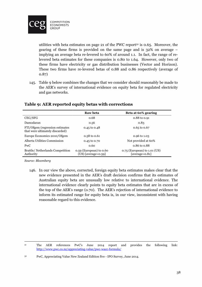
38

utilities with beta estimates on page 21 of the PWC report52 is 0.65. Moreover, the gearing of these firms is provided on the same page and is 32% on average – implying an average beta re-levered to 60% of around 1.1. In fact, the range of re-levered beta estimates for these companies is 0.80 to 1.64. However, only two of these firms have electricity or gas distribution businesses (Vector and Horizon). These two firms have re-levered betas of 0.88 and 0.86 respectively (average of 0.87)

145. Table 9 below combines the changes that we consider should reasonably be made to the AER’s survey of international evidence on equity beta for regulated electricity and gas networks.

Table 9: AER reported equity betas with corrections

Raw beta Beta at 60% gearing

CEG/SFG 0.68 0.88 to 0.91

Damodaran 0.56 0.83

FTI/Ofgem (regression estimates that were ultimately discarded)

0.45 to 0.48 0.65 to 0.67

Europe Economics 2010/Ofgem 0.58 to 0.61 0.96 to 1.03

Alberta Utilities Commission 0.45 to 0.70 Not provided at 60%

PwC 0.60 0.86 to 0.88

Brattle/ Netherlands Competition Authority



Source: Bloomberg

146. In our view the above, corrected, foreign equity beta estimates makes clear that the new evidence presented in the AER’s draft decision confirms that its estimates of Australian equity beta are unusually low relative to international evidence. The international evidence clearly points to equity beta estimates that are in excess of the top of the AER’s range (o.70). The AER’s rejection of international evidence to inform its estimated range for equity beta is, in our view, inconsistent with having reasonable regard to this evidence.

51 The AER references PwC's June 2014 report and provides the following link:

http://www.pwc.co.nz/appreciating-value/pwc-wacc-formula/

52 PwC, Appreciating Value New Zealand Edition five - IPO Survey, June 2014.

39

5.2 International precedent for the use of foreign

comparators

147. We have conducted a review of the recent regulatory decisions made by regulators in Australia and in 8 other countries. Within Australia, only the ERA did not refer to the equity betas of foreign companies.

148. In foreign jurisdictions that used the CAPM and subsequently derived a beta estimate from a sample of comparators, we found that the regulators almost always included foreign firms in their sample. The remaining regulators that did not obtain their own sample of comparators were nevertheless influenced by the equity betas of foreign firms, either by referring to reports from their consultants that were based on data including foreign firms, or by referring to the equity beta decisions of other regulators.

149. The remainder of this section sets out the findings of our review, with a summary provided in Table 10.

40

Table 10: Usage of foreign firms in the sample of comparators

Australia Regulator Usage of foreign firms

New South Wales IPART Comparators consist of 8 Australian firms, 6 UK firms, and 64 US firms.

Victoria ESC Had regard to equity beta estimates of relevant foreign entities, and referred to consultant reports containing beta estimates of US firms.

Queensland QCA Comparators include 9 Australian firms, 3 UK firms, and 20 US firms.

Western Australia ERA Sample had 14 Australian firms, and no foreign comparators.

Foreign Regulator Usage of foreign firms

New Zealand ComCom The comparator sample had 2 New Zealand firms, 6 from Australia, 1 from UK, and 70 US firms.

United Kingdom Ofgem Electricity decision: Sample had 7 UK firms and 1 international comparator

Gas decision: Relied on consultant reports with international firms in Europe, and some with operations in multiple countries.

Alberta, Canada AUC The Commission considered beta estimates by five consultants, accepted one as a lower bound, and another as an upper bound. The upper bound estimate was based on three proxy samples, with the sample that included foreign firms convincing the consultant that estimates based exclusively on Canadian firms were too low – a view that was shared by the consultant who recommended the lower bound estimate.

Singapore EMA Sample had two US firms and one each from UK, Spain, and Canada.

Germany BNetzA The sample included three US firms, two each from Spain, UK, and Italy, and one from New Zealand.

France CRE Referred to beta values that other European regulators had adopted.

Sweden Ei Relied on reports that featured international comparators.

Netherlands ACM Heat distribution and supply: Obtained two samples. The first contained five firms, with 3 from Czech Republic, 1 from Germany, and 1 from Poland. The latter consisted of 18 firms, with 6 from UK, 6 from USA, 2 from Spain, 2 from Italy, and 1 each from Portugal and Canada. Gas and electricity distribution: There were 14 firms in the sample, with 4 from USA, 4 from UK, 3 from Canada, 2 from Australia, and 1 from Spain.

5.2.1 Australian jurisdictions

5.2.1.1 New South Wales – IPART

150. In its review of regulated retail prices for electricity for the 2013 – 2016 period, IPART selected a sample of 78 diversified electricity firms, classified according to the Standard Industry Classification (SIC) and Global Industry Classification Standard (GICS). The sample consisted of 8 Australian firms, 6 UK firms, and 64 US firms.53

151. IPART also selected a separate sample of 25 electricity generation businesses in order to validate their gearing ratio and equity beta estimates. The sample

53 IPART, Review of regulated retail prices and charges for electricity from 1 July 2013 to 30 June 2016,

2013, p. 196-198

41

contained 3 Australian firms, 7 UK firms, 4 US firms, 9 Canadian firms, and 2 firms from New Zealand.54

5.2.1.2 Victoria – ESC

152. The ESC’s draft decision for electricity distribution in Victoria for the 2006 – 2010 period referred to empirical evidence from both Australian and foreign markets in order to obtain a suitable equity beta. It also relied on its own previous reviews, as well as the equity beta values adopted by other regulators.55

153. In its final decision, the ESC justified its approach on the basis that weight should be placed on all available information:

“the Commission has also had regard to estimates of equity betas for

relevant entities in other countries, the equity beta estimates used by

regulators in other countries (to the extent that the CAPM is used),

previous decisions by Australian regulators and the qualitative arguments

presented, thus augmenting the information available from Australian

empirical evidence. The Commission would expect to continue to place

weight on all of the available information when deriving the equity beta

for regulated entities.”56

154. Furthermore, the ESC noted that analysing the equity betas of electricity distribution firms in the US “has the advantage of being able to make use of a much large set of listed entities, as well as information over a longer period”.57 The final decision also had regard to reports by Gray and Officer (2004),58 and Lally (2005),59 both of which made reference to the equity beta of US firms.

54 Ibid, p. 198-199

55 Essential Services Commission, Electricity Distribution Price Review 2006 – 10, October 2006 Final Decision, 2006, p. 347

56 Ibid, p. 352

57 Ibid, p. 351

58 Gray and Officer, The Equity Beta of an Electricity Distribution Business: Draft Report Prepared for CitiPower Ltd & PowerCor Australia Ltd, 12 November 2004

59 Lally, The Equity Beta for ETSA Utilities, 6 May 2005

42

5.2.1.3 Queensland – QCA

155. The QCA’s practice is to obtain beta estimates from a comparative sample containing both local and international water and energy firms, which it selected “because of their perceived similar systematic risk characteristics”.60

156. It also previously used a similar approach in its price monitoring assessment of water and wastewater prices in 2011. Its sample of comparator companies included 3 UK water companies, 9 US water companies, 9 Australian energy network companies, and 11 US electric utilities,61 with the equity beta being calculated in Lally (2010).62

5.2.1.4 Western Australia – ERA

157. For its assessment of the access arrangement for the Western Power network, the ERA established a sample of comparator companies with assistance from Professor Henry of the University of Melbourne. The sample contained 14 Australian firms and no foreign firms.

158. The ERA recognised that the available data for Australian firms was highly limited, and thus included gas and general utility businesses in its sample, arguing that the gas network businesses were reasonable albeit imperfect comparators to electricity network businesses.63

5.2.2 Foreign jurisdictions

5.2.2.1 New Zealand Commerce Commission

159. In 2010, the Commerce Commission in New Zealand reviewed its input methodologies for electricity distribution and gas pipeline services. The Commission’s approach to obtaining equity betas involved identifying a sample of relevant comparator firms, both in New Zealand and overseas, that were in the same

60 Queensland Competition Authority, SEQ Retail Water Long-Term Regulatory Framework – weighted

average cost of capital (WACC), 2014, p. 23.

61 Queensland Competition Authority, SEQ Interim Price Monitoring for 2010/11 Part B – Detailed

Assessment, February 2011, p. 212

62 Lally, The Estimated WACC for the SEQ Interim Price Monitoring, 2010

63 Economic Regulation Authority, Final Decision on Proposed Revisions to the Access Arrangement for the Western Power Network, 2012, p. 397

43

service being evaluated, and had a similar risk profile.64 The sample featured 2 New Zealand firms, 6 from Australia, 1 from UK, and 70 US firms.65

160. The Commission’s reasoning was that most New Zealand industries did not have a sufficient number of comparable businesses to allow the Commission to implement its approach by relying solely on domestic data. The commission further relied on advice by Dr Lally, who incorporated US electricity and gas utilities into his analysis. Dr Lally further argued that US firms from both sectors were comparators for each other because the sectors appeared to have similar activities and regulations. This allowed data from both groups of US firms to be used to draw conclusions about asset beta for New Zealand gas and electricity lines businesses.66

5.2.2.2 United Kingdom – Ofgem

Electricity

161. Ofgem’s decision on the appropriate asset beta to be used in the Distribution Price Control Review 5 (DPCR5) referred to evidence from a sample of 8 companies that were comparable to the distribution network operators in question. Although Ofgem did not explicitly use the estimated equity beta from the sample, it is clear that it was nevertheless influenced by it.

162. The sample consisted of 7 UK firms (3 energy and 4 water businesses) and one international comparator (AGL resources). In making its decision, Ofgem highlighted the simple average of the betas for the firms in the sample.67

Gas

163. In its report on the financial and uncertainty aspects of its approach towards gas distribution price controls from 2013 to 2021, Ofgem referred to reports by three of its consultants, including one by Europe Economics.68

164. Europe Economics assessed the betas for three companies that are all listed in the UK. However, Europe Economics further referred to a sample of foreign comparators in order to establish the robustness of its analysis. Most of the comparators were European companies, with some operating in multiple countries

64 Commerce Commission, Input Methodologies (Electricity Distribution and Gas Pipeline Services):

Reasons Paper, December 2010, pp. 510-512.

65 Ibid, p. 518

66 Ibid, p. 514-515

67 Ofgem, Electricity Distribution Price Control Review Final Proposals – Allowed Revenues and Financial issues, December 2009, p. 14

68 Ofgem, RIIO-GD1: Final Proposals – Finance and uncertainty supporting document, 2012

44

outside Europe, including North America, South America, Africa, and the Asia Pacific region.69

5.2.2.3 Alberta, Canada – Alberta Utilities Commission

165. The Commission considered the analysis of five consultants in coming up with its beta estimate before adopting one recommendation by Dr Booth as the lower bound and another by Dr Vilbert as the upper bound.70

166. While Dr Booth’s analysis was based only on Canadian utility holding companies, Dr Vilbert referred to three proxy groups to obtain his estimates – a Canadian utilities sample, a gas distribution company sample with both Canadian and US companies, and another sample of pipelines with Canadian and US companies. Dr Vilbert subsequently found that the estimates from the Candian sample produced betas that were underestimated, and modified them upwards.71

167. It can therefore be seen that although the Commission did not create its own sample of comparator firms, it was nonetheless influenced by estimates from foreign firms, which suggested that the betas obtained from Canadian firms alone were “not adequately representative of forward looking expectations”.72

5.2.2.4 Singapore – Energy Market Authority

168. The Authority’s review of the Long Run Marginal Cost parameters for setting contract prices uses an equity beta estimated from a sample of comparator companies. The sample consists of five companies, with two US firms, and one each from UK, Spain, and Canada. It is particularly notable that the sample does not contain any domestic firms in Singapore.73

5.2.2.5 Germany – Bundesnetzagentur

169. The Bundesnetzagentur calculated the CAPM beta by referring to a peer group of nine companies with comparable risk to the electricity transmission system

69 Europe Economics, The Weighted Average Cost of Capital for Ofgem’s Future Price Control, Final

Phase I Report, 2010, pp. 38-42

70 Alberta Utilities Commission, 2009 Generic Cost of Capital, November 2009, p. 70

71 Ibid, pp. 67 – 68

72 Ibid, p. 70

73 Energy Market Authority, Review of the Long Run Marginal Cost (LRMC) Parameters for Setting the

Vesting Contract Price for the Period 1 January 2013 to 31 December 2014, Final Determination Paper, 30 Sep 2012, Appendix D.

45

operators that it was regulating. It defined “comparable risk” according to the criterion of 75% network operation.

170. The sample included three US firms, two each from Spain, UK, and Italy, and one from New Zealand. The regulator further noted that including a number of countries allowed “one-sided distortion” to be avoided.74

5.2.2.6 France – Commission de régulation de l'énergie

171. The Commission obtained the cost of capital for electricity firms based on a study by an external consultant, as well the beta values for electricity that other European regulators had adopted.75

172. Although the report by the external consultant and the list of European regulators considered are not available, it is nevertheless clear that the Commission had been influenced by the beta values of foreign companies.

5.2.2.7 Sweden – Swedish Energy Market Inspectorate

173. The Inspectorate relied on reports by Grant Thornton and Ernst & Young to estimate beta as part of WACC calculations. The reports referred to international comparators, with Grant Thornton arguing that betas of internationally comparable listed companies provided a measure of how a sector compared to other markets in terms of risk.

174. In choosing to use the MSCI EAFE (Morgan Stanley Compsite Index – Europe, Australasia, Far East), Grant Thornton further argued that a broader international index for developed countries had a higher correlation with the Swedish stock market as compared to an index for an individual market.76

5.2.2.8 Netherlands – Energiekamer and Dutch Energy Regulator

Heat distribution and supply (Energiekamer)

175. Energiekamer engaged Oxera to estimate the cost of capital for heat distribution and supply activities in the Netherlands. As part of the calculations, Oxera obtained

74 Bundesnetzagentur, Economic regulation of TSOs: The regulatory framework in Germany,

presentation by Dr Annegret Groebel, FSR Workshop, Florence, 21 October 2011, p. 31

75 Commission de régulation de l'énergie, Délibération de la Commission de régulation de l’énergie du 12 décembre 2013 portant décision relative aux tarifs d’utilisation d’un réseau public d’électricité dans le

domaine de tension HTA ou BT, p. 20

76 Grant Thornton, Estimering av kalkylränta (WACC) för elnätsverksamhet under tillsynsperioden

2012-2015, April 2011, p. 13.

46

the asset beta of comparator companies, which were chosen based on similarity in terms of business characteristics, regulatory features, and residual risk exposure.

176. Oxera obtained two separate samples, one for heat network comparators, and one for regulated comparators. The former contained five firms, with three from Czech Republic, one from Germany, and one from Poland. The latter consisted of 18 firms, with 6 from UK, 6 from USA, 2 from Spain, 2 from Italy, and one each from Portugal and Canada.77

Gas and electricity distribution (Dutch Energy Regulator)

177. In its advice to the Dutch Energy Regulator, Frontier Economics selected a set of comparator companies for the purpose of calculating the relevant asset beta to be used as part of the calculation of the cost of capital for regional distribution networks.

178. There were 14 firms in the sample, with 4 from USA, 4 from UK, 3 from Canada, 2 from Australia, and 1 from Spain.78

5.3 The impact of the resources sector on energy network

equity betas

179. The AER asked Professor Ólan Henry to estimate betas for Australian comparators for three different time periods being: the longest time period; the period after the tech boom and excluding the GFC; and the last five years of data.79

180. Henry defined all of these periods to end in June 2013:

� the longest period differs depending on the firm in question but for 8 out of the 9 firms data becomes available in mid-2000 or later;

� the tech boom is defined as running from 1 July 1998 to 31 December 2001

(this was an instruction to Henry from the AER);

� the GFC is defined as running from 1 September 2008 to October 2009.

181. If the shocks hitting the equity market during the GFC and/or the technology boom are not representative of the market conditions that investors expect in the future then it follows that the beta measured in those periods will not be a good proxy for investor’s forward-looking expected beta.

77 Oxera, The cost of capital for heat distribution and supply, Final report prepared for Energiekamer,

September 2009, pp. 11-12.

78 Frontier Economics, The cost of capital for Regional Distribution Networks, a report for DTE, December 2005, p. 44

79 Henry, op cit, p. 11

47

182. The AER has instructed Henry to exclude the GFC and/or the technology boom from the analysis for this reason. However, over the period analysed by Henry the unprecedented mining boom was as significant an impact on the Australian equity market as the other two events. This is clearly illustrated in Figure 9 below.

Figure 9: ASX 200 from 1992 to 2014

Source Bloomberg AS51 index, CEG analysis.

183. The impact of the mining boom on the Australian equity market can be seen by the run up in market valuations from 2004 until the GFC. Moreover, much of the fall in equity prices subsequent and during the period thought of as the “GFC” actually represents a dramatic fall in commodity prices. On the basis of Figure 9, the mining boom would appear to have much greater claim to being exceptional than the ‘tech boom’, which appears to have had little impact upon the valuation of the main Australian share market index. In addition, Henry’s definition of the ‘GFC’ only captures around half the fall in equity valuations from their peak

184. These trends in equity market valuations can also be illustrated by examining non-rural commodity prices. From 2000 onwards there was a significant increase in both the rate of growth and the volatility of commodity prices (see Figure 10 below). The non-rural commodity price index published by the Reserve Bank of Australia (RBA) reached a peak in November 2008 (148.4) which was nearly four times

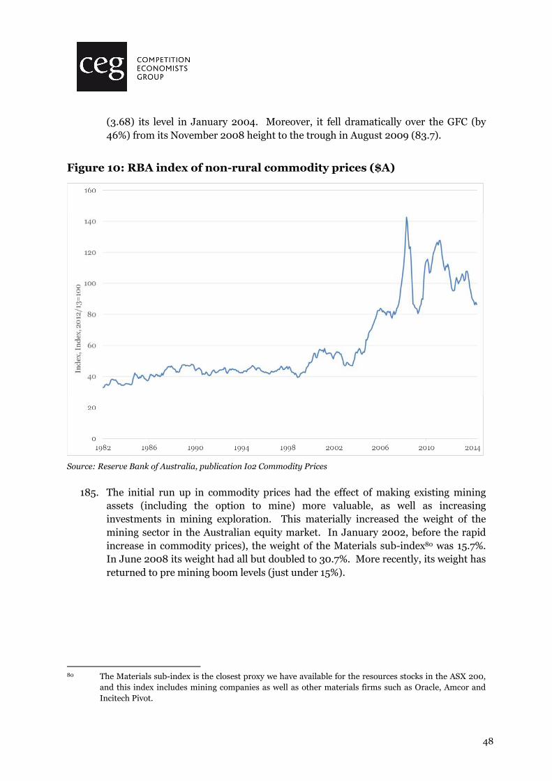
48

(3.68) its level in January 2004. Moreover, it fell dramatically over the GFC (by 46%) from its November 2008 height to the trough in August 2009 (83.7).

Figure 10: RBA index of non-rural commodity prices ($A)

Source: Reserve Bank of Australia, publication Io2 Commodity Prices

185. The initial run up in commodity prices had the effect of making existing mining assets (including the option to mine) more valuable, as well as increasing investments in mining exploration. This materially increased the weight of the mining sector in the Australian equity market. In January 2002, before the rapid increase in commodity prices), the weight of the Materials sub-index80 was 15.7%. In June 2008 its weight had all but doubled to 30.7%. More recently, its weight has returned to pre mining boom levels (just under 15%).

80 The Materials sub-index is the closest proxy we have available for the resources stocks in the ASX 200,

and this index includes mining companies as well as other materials firms such as Oracle, Amcor and Incitech Pivot.

49

Figure 11: Materials index as a proportion of ASX200

Source: Bloomberg, CEG analysis

186. The growth in the resources sector was associated with unprecedented volatility in both commodity prices (as described in Figure 10) above and volatility in equity prices for firms in the Materials sub-index (as illustrated in Figure 12 below). This volatility for the Materials sub-index was much higher than that observed for the ASX 200 as a whole. This is illustrated in Figure 12, which shows the annual variance in the daily returns on Materials sub-index of the ASX 200, the ASX 200, and the ASX 200 net of the Materials sub-index.

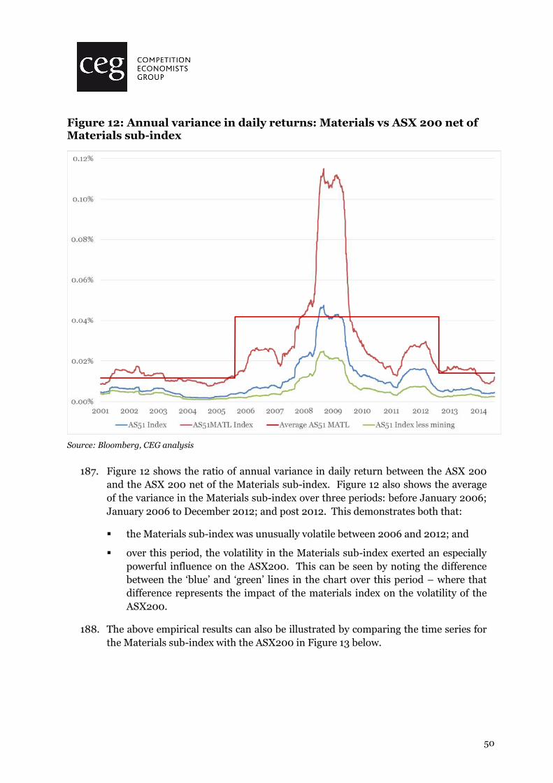
50

Figure 12: Annual variance in daily returns: Materials vs ASX 200 net of Materials sub-index


187. Figure 12 shows the ratio of annual variance in daily return between the ASX 200 and the ASX 200 net of the Materials sub-index. Figure 12 also shows the average of the variance in the Materials sub-index over three periods: before January 2006; January 2006 to December 2012; and post 2012. This demonstrates both that:

� the Materials sub-index was unusually volatile between 2006 and 2012; and

� over this period, the volatility in the Materials sub-index exerted an especially powerful influence on the ASX200. This can be seen by noting the difference between the ‘blue’ and ‘green’ lines in the chart over this period – where that difference represents the impact of the materials index on the volatility of the ASX200.

188. The above empirical results can also be illustrated by comparing the time series for the Materials sub-index with the ASX200 in Figure 13 below.

51

Figure 13: Materials sub-index vs ASX 200


189. The increased volatility and weight of resource stocks over the period January 2006 to December 2012 suggests that betas of non-resources stocks are likely to have been depressed relative to the ASX 200. That is, higher volatility in resources stocks is likely to be driving higher variance in the ASX 200 as well as a higher co-variance of the resources sector with the market index. This would drive up betas for the resources sector and drive down betas for the non-resources sector.

5.3.1 Interpretation of betas affected by mining boom

190. As we note below, the measured equity betas for mining stocks were extremely high during the period 2006 to 2012. This is not surprising. However, the mathematical definition of beta is such that it must sum to 1.0 across all firms.81 It follows that high mining stock betas must depress betas for all other firms on average. That is, equity betas for other sectors must be lower over the same period.

191. Investors will only rationally believe that lower measured betas for non-mining stocks over this period reflect lower levels of forward looking beta if they believe

81 Reflecting the fact that equity beta measures relative risk and the average equity beta must be equal to

1.0.

52

that the market conditions under which they were estimated are expected to be typical of future market conditions. This is not a plausible assumption. Investors may not rule out the possibility of another ‘once in a life time’ rise and fall in commodity prices over the next 5-10 years but they certainly will not expect it to occur.82

192. This means that betas measured over the period of the mining boom and subsequent bust must be interpreted warily. All other betas, including but not restricted to regulated utility betas, will be depressed by heightened betas for (and heightened weight of) mining stocks. It is only reasonable to include the effect of this depression in non-mining betas in a forward-looking estimate of beta if one reasonably believes that investors anticipate similar market conditions prospectively.83

193. Figure 14 illustrates the impact described above by calculating the average beta of the Materials sub-index and comparing this to the average beta of all other ASX sub-indices. This time series clearly shows that the betas of all sectors of the ASX 200 less the Materials sector have been depressed by the mining boom.

82 Even if they did, then the MRP consistent with this assumption would be elevated because mining stocks

tend, even in normal periods, to have higher risk premiums. An increase in the weight of mining stocks in the index would, other things equal, increase the average risk of the index.

83 Even then, a higher MRP would be appropriately matched to that beta estimate (see footnote above).

53

Figure 14: Beta estimate materials sub-index vs. all other sub-indices

Source: Bloomberg, CEG analysis. Betas are daily betas with 500 observations (roughly 2 year betas)

194. The period from 2004 to 2008 is most striking in this figure. It shows exceptionally elevated betas for the Materials sub-index and an offsetting depression in betas for all other firms. The offsetting fall in non-Materials betas is smaller given than the rise in Materials betas because the Materials sector is only between 20% and 30% (averaging around 25%) of the overall ASX200 index. Consequently, a 0.8 rise in beta for the materials index (which is the increase from July 2002 to July 2006) will tend to depress the beta of the non-Materials sector by about 0.2 (=0.8*(1-25%)). This is the size of the depression in non-Materials betas measured in July 2007.84

5.3.2 Interpretation of betas affected by mining boom and GFC

195. The same analysis that was performed in Figure 14 is performed in Figure 15 below except in this analysis the Financials sub-index and Materials sub index are

84 It can be seen that the two lines in the above graph are reasonably close, but imperfect, mirror images of

each other. The two lines would, as a matter of mathematical construction, appear identical mirror images of each other if the Materials sub-index had an approximately constant 50% weight in the ASX200. However, they are imperfect mirror images because the relative weights are neither equal not constant through time (i.e., the Materials index weight varies from 15% to 30% and back to 15% over the period).

54

combined in order to examine the combined impact of both the mining boom and the GFC on the betas of all other stocks (i.e., stocks that are not in either of the Materials or the Financials sub-indices).

Figure 15: Beta estimate for material and financial sub-indices vs. all other sub-indices


196. This figure underlines the fact that since 2004 the combined effect of the mining boom and the GFC has been to significantly depress the betas of all other stocks in the ASX200. The average beta of all other stocks has been depressed by an average of more than 0.2 over this entire period and the average betas are only now returning to pre mining boom/GFC levels.

5.3.3 Implications for estimating forward looking betas

197. The fundamental conclusion of this analysis is that the betas for all firms not in the Materials/Financial sub-indices measured over this period, especially the period 2004 to 2008, were depressed by the exceptionally high betas of the Materials and Financial indices. This applies to utilities but not solely to utilities.

198. Betas (for non-mining firms and non-financial firms) measured over this period will be depressed. It will only be appropriate to include this depressed effect on betas in

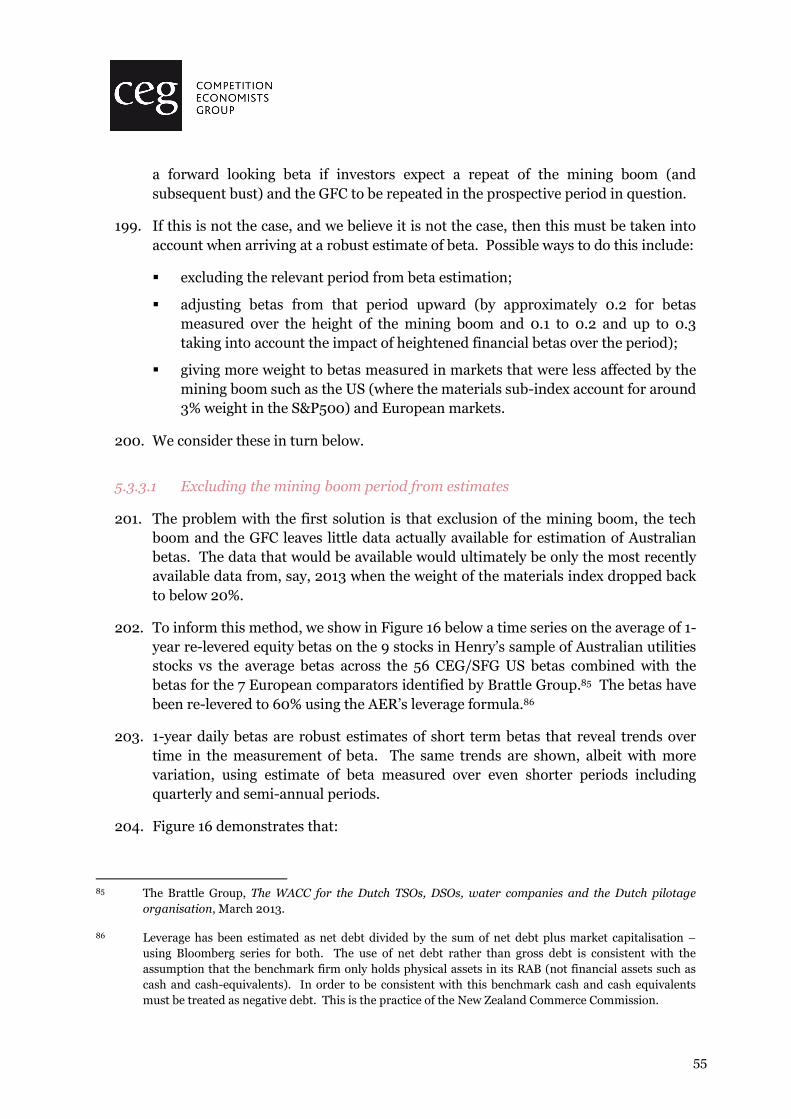
55

a forward looking beta if investors expect a repeat of the mining boom (and subsequent bust) and the GFC to be repeated in the prospective period in question.

199. If this is not the case, and we believe it is not the case, then this must be taken into account when arriving at a robust estimate of beta. Possible ways to do this include:

� excluding the relevant period from beta estimation;

� adjusting betas from that period upward (by approximately 0.2 for betas measured over the height of the mining boom and 0.1 to 0.2 and up to 0.3 taking into account the impact of heightened financial betas over the period);

� giving more weight to betas measured in markets that were less affected by the mining boom such as the US (where the materials sub-index account for around 3% weight in the S&P500) and European markets.

200. We consider these in turn below.

5.3.3.1 Excluding the mining boom period from estimates

201. The problem with the first solution is that exclusion of the mining boom, the tech boom and the GFC leaves little data actually available for estimation of Australian betas. The data that would be available would ultimately be only the most recently available data from, say, 2013 when the weight of the materials index dropped back to below 20%.

202. To inform this method, we show in Figure 16 below a time series on the average of 1-year re-levered equity betas on the 9 stocks in Henry’s sample of Australian utilities stocks vs the average betas across the 56 CEG/SFG US betas combined with the betas for the 7 European comparators identified by Brattle Group.85 The betas have been re-levered to 60% using the AER’s leverage formula.86

203. 1-year daily betas are robust estimates of short term betas that reveal trends over time in the measurement of beta. The same trends are shown, albeit with more variation, using estimate of beta measured over even shorter periods including quarterly and semi-annual periods.

204. Figure 16 demonstrates that:

85 The Brattle Group, The WACC for the Dutch TSOs, DSOs, water companies and the Dutch pilotage

organisation, March 2013.

86 Leverage has been estimated as net debt divided by the sum of net debt plus market capitalisation – using Bloomberg series for both. The use of net debt rather than gross debt is consistent with the assumption that the benchmark firm only holds physical assets in its RAB (not financial assets such as cash and cash-equivalents). In order to be consistent with this benchmark cash and cash equivalents must be treated as negative debt. This is the practice of the New Zealand Commerce Commission.

56

� over time there has been an upward trend in average re-levered equity betas on these stocks – and most recently these estimates have been around 0.8;87 and

� over time there has also been variation in the average level of beta. Some of this variation has been due to the entry and exit of firms from the average. The variation is also due to changing market circumstances.

Figure 16: 1-year daily betas on Australian utilities stocks vs US and European betas


205. Both Australian and foreign equity began the last decade low as a result of the impact of the technology bubble. However, unlike foreign utility comparators, whose betas averaged 0.95 from 2003 onwards, Australian utility betas failed to recover from their technology bubble lows due, in our view, to the emergence of the mining boom in Australia.

206. The recent data suggests that, post mining boom and GFC, equity betas on Australian utilities stocks are higher than at any point in history. It also suggests that the difference between Australian and foreign betas has reduced dramatically relative to its height (which was during the height of the Australian mining boom).

87 The figures for the last two years ending 11 December 2014/2013 are 0.73/0.78

0.0

0.2

0.4

0.6

0.8

1.0

1.2

1.4

1.6

2000 2001 2002 2003 2004 2005 2006 2007 2008 2009 2010 2011 2012 2013 2014

Australia Difference Other

57

207. This raises concerns about relying on estimates of equity beta estimated over a longer time period capturing market conditions that may not be relevant to the future period. This is less true in the context of foreign beta estimates, which are less affected by the unprecedented commodity price boom and fall.

208. This analysis suggests that a reasonable range for Australian comparator equity betas over the last ten years is 0.6 to 0.8. However, this does not have regard to foreign betas or the depressing effects of the mining boom on Australian betas. The AER’s range of o.4 to 0.7 for the benchmark regulated business would only be reasonable on this representation of the data if:

� zero weight was given to foreign betas; and

� significant weight was given to Australian betas in the period prior to 2004. This is a period when there were at most 5 comparators and a period that is affected by the technology bubble.88

209. We do not consider either of these approaches is reasonable. We consider that the data shown in Figure 16 supports a beta estimate of 0.8 as reasonable. This is consistent with the weight of all the most recent beta estimates (Australian and US). It is also consistent with, but lower than, the average of these over the last 10 years.

5.3.3.2 Implementation of an adjustment

210. The second approach is possible but will inevitably result in somewhat arbitrary assumptions in the implementation of such an adjustment and the nature of such adjustments will have complex interactions with other adjustments – such as the exclusion of the GFC. We note that the AER has a similar view on equity betas estimated in foreign jurisdictions:89

If foreign comparators were to be used to determine the equity beta

estimate for the benchmark efficient entity, it would be reasonable to

quantify the impacts of these differences and to make necessary

adjustments. However, it is difficult to make such adjustments in a robust

and transparent manner.

211. The AER appears to take from this analysis that it is not reasonable to consider foreign equity betas in determining the range for the equity beta for the benchmark firm because there may be reason to believe that there is a difference (albeit unquantifiable) between these estimates and the beta on the benchmark firm. The fallacy of this conclusion is shown by attempting to apply the same logic to the equity beta for Australian firms estimated in market conditions that are different

88 Which the AER instructs Henry is 3 July 1998 to 28 December 2001


58

from those that are expected to apply in the future. Following this logic would result in an empty set of reasonable equity beta comparators.

212. The analysis in Figure 14 and Figure 15 suggests an upwards adjustment of between 0.1 to 0.3 to Australian betas measured over the last 10 years would be appropriate in order to adjust for the effect of the mining boom. This would raise SFG’s estimate of Australian betas from 0.58 to a range of 0.68 to 0.88.

5.3.3.3 Considering foreign estimates of equity beta

213. The third approach is essentially consistent with Networks NSW proposed approach to give weight to equity betas estimated from United States firms (and possibly European firms) in addition to those from Australian firms.

214. In light of the findings of sections 5.1 and 5.3, we also consider it worthwhile to revisit SFG’s decision to give double weight to estimates of equity beta from Australian firms. We consider that the problems with using historical Australian betas measured over the mining boom as proxies for expected future betas may suggest that it is not appropriate to give them higher weight than foreign betas. For SFG’s sample, giving Australian betas the same individual weight as United States betas gives rise to an average estimate of equity beta of 0.85.

5.3.4 Summary

215. In our view, the best evidence suggests a value for beta for the benchmark regulated firm that is in excess of 0.80.

59

Appendix A Factors lowering CGS yields post GFC

A.1 RBA and Treasury/AOFM letters

216. In response to a report written for the Victorian gas businesses in 2012,90 the AER sought two letters from the RBA and Treasury/AOFM91. The Victorian gas draft decision refers to these letters as support for rejecting arguments that CGS is not the best proxy for the risk free rate. However, this is not a position that we put then or that we put now. In our view, these letters provide support for our firm view that the factors driving down CGS yields cannot be presumed to be driving down equity yields.

217. The content of these letters is strongly supportive of our views. Specifically:

� Increased demand for CGS is driven by increased levels of risk/risk aversion leading to a ‘flight to quality’.

� RBA paragraph 2 on page 1, first sentence.

� Treasury/AOFM paragraph 3 on page 1. Also, paragraph 2 under the first question answered on page 2.

� A factor contributing to the elevated demand for CGS is the reduced supply of alternative AAA rated liquid government bonds. Hence, there has been heightened demand for CGS by foreigners.

� RBA paragraph 2 on page 1, second sentence.

� Treasury/AOFM paragraphs 3 and 4 under the first question answered on page 2. The AOFM states:

The weak and fragile global economy has put downward pressure

on benchmark global long-term bond yields, and is driving investors

into high quality government debt. As a result, Australia is

reaping the benefits of a deep and liquid AAA-rated CGS

market that is attracting strong demand from

international investors. [Emphasis added.]

90 CEG, 'Internal consistency of risk free rate and MRP in the CAPM', March 2012.

91 RBA, Letter regarding the Commonwealth Government Securities Market, Guy Debelle, Assistant Governor, Financial Markets, Reserve Bank of Australia, 16th July 2012, p. 1–2.

Australian Government, The Treasury, Letter to Joe Dimasi, ACCC, regarding the Commonwealth

Government Securities Market, 18th July 2012.

60

� Risk premiums for other assets, including but not restricted to equities, measured relative to the CGS have increased as part of the same ‘flight to quality’.

� RBA paragraph 2 on page 1, in particular the last two sentences. Note the last sentence:

“This widening indeed confirms the market's assessment of the

risk-free nature of CGS and reflects a general increase in risk

premia on other assets.”

We regard this as a clear statement in support of our central position.

� Treasury/AOFM final paragraph under the first question answered on page 2.

� As a general rule market risk premia are unstable and adding a fixed MRP to a floating CGS yield cannot be presumed to give accurate results. An important cross-check is provided by asking whether the assumption of a fixed MRP is consistent with the observed changes in risk premiums on debt.

� RBA last two paragraphs on page 1 (including overleaf to page 2).

218. Notably, the AER interprets the last two paragraphs on page 1 of the RBA letter in a different manner than we do above. In order to describe why we believe the AER’s interpretation is incorrect, consider the two paragraphs from the RBA letter in question:

I therefore remain of the view that CGS yields are the most appropriate

measure of a risk-free rate in Australia.

That said, market risk premia are unlikely to be stable through time.

While it is a reasonably simple matter to infer changes in debt risk premia

from market prices, it is less straightforward to do so for equity premia.

In making use of a risk-free rate to estimate a cost of capital, it is

important to be mindful of how the resulting relativity between the cost

of debt and that of equity can change over time and whether that is

reasonable.

A.2 IMF assessment of factors driving down safe asset

yields

A.2.1 Shrinking supply of safe sovereign debt

219. In April 2012, the IMF released a detailed analysis of factors driving down the yields on safe assets worldwide (i.e., not just in Australia). The IMF summarised its analysis in the following manner:

61

On the supply side, concerns about high government debts and deficits

in some advanced economies have reduced the perceived safety of

government debt. Recent rating downgrades of sovereigns, previously

considered to be virtually riskless, show that even highly-rated assets are

subject to risks.

The number of sovereigns whose debt is considered safe has fallen. IMF

estimates show that safe asset supply could decline by some $9 trillion—or

roughly 16 percent of the projected sovereign debt—by 2016. Private sector

issuance of safe assets has also contracted sharply on poor securitization

practices in the United States.

Safe asset scarcity will increase their price, with assets perceived as the

safest affected first. Investors unable to pay the higher prices would have

to settle for assets that have higher levels of risk.92

220. Put simply, the amount of sovereign debt that investors perceive as safe has dramatically declined with the Eurozone debt crisis.

221. The demand for Australian CGS has benefited from this reduction in the perceived safety of other sovereigns’ debts. The relatively strong fiscal position of the Australian Commonwealth Government is illustrated in the IMF chart below.

92 See IMF summary at: http://www.imf.org/external/pubs/ft/survey/so/2012/POL041112A.htm.

62

Figure 17: IMF estimates of Sovereign indebtedness relative to GDP

222. We have accessed the latest IMF forecasts of gross debt to GDP, from the IMF 2014 World Economic outlook, and have created the same chart as forecast by the IMF in 2019 – see Figure 18 below (with Australia highlighted). This tells essentially the same story – gross Government debt in Australia is very small fraction of GDP relative to other developed countries and is expected to remain so for the foreseeable future.

63

Figure 18: IMF estimates of Sovereign indebtedness relative to GDP

Source: IMF, CEG analysis

223. Australian CGS are now amongst very few developed country government bonds that have a AAA credit rating from S&P. The downgrade of US and French Government debt in 2011 (preceded by downgrades to most other Eurozone Government debt) left Australia one of only a very small club of AAA rated sovereigns.93 This has been associated with a significant increase in demand for CGS by foreign institutions looking for AAA rated sovereign debt.

224. The head of the Australian Office of Financial Management (AOFM) has been quoted in the press explaining the fall in CGS yields as not just a flight from equities but also as a spill-over from the reduction in the availability of AAA rated government debt in the rest of the developed world. RBA Assistant Governor, Guy Debelle, was quoted in the same article commenting on increased demand for CGS from foreigners:94

93 The others being Canada, Denmark, Finland, Germany, Luxemburg, Netherlands, Norway, Singapore,

Sweden, Switzerland and the UK.

94 The Age, Australia reaps bond windfall, Tim Colebatch, 16 February 2012, available at: http://www.theage.com.au/opinion/political-news/australia-reaps-bond-windfall-20120215-1t6q2.html#ixzz1oQQsnHCl.

64

“It's the product of a whole lot of influences,” he said. ''Australia is a AAA-

rated sovereign, and that's a shrinking club. Investors might be taking

money out of equity markets and putting it into the safety of bonds paying

fixed interest.

“There have been changes in currency level and hedging costs. It's not

surprising that demand for Australian government securities should have

risen in the current circumstances.”

Reserve Bank assistant governor Guy Debelle said this week the demand

for Australian bonds was coming largely from the sovereign wealth funds

of foreign governments.

Mr Debelle said the Reserve estimated that 75 per cent of Australian bonds

were owned offshore. He said foreign demand for Australian bonds could

be partly responsible for the recent strength of the Australian dollar.

225. It is clear that the IMF, the AOFM and the RBA95 all believe the shrinkage in the supply of safe sovereign debt globally is raising demand for the ‘shrinking pool’ of remaining safe sovereign debt – of which Australian CGS are a part. However, the key question is whether this is also leading to heightened demand for Australian listed equities. If the answer is ‘no’ then it is wrong to assume that historically depressed CGS yields are associated with historically depressed required equity returns (i.e., with a constant spot MRP).

226. In our view it is clear that this is not the case and this is consistent with the commentary of the IMF, AOFM and RBA. 96

A.2.2 Shrinking supply of safe private debt (and inability to manufacture

more)

227. The IMF also notes that the shrinking supply of safe sovereign debt has happened at the same time at which the perceived supply of safe private sector debt has also collapsed. Prior to the GFC there was a large supply of highly rated private sector debt which investors regarded as substitutable for safe sovereign debt. However, as the IMF notes:97

The production of safe assets by the private sector largely collapsed with

the onset of the global crisis. Total private sector securitization issuance

95 In addition to the above quote from RBA Assistant Governor Guy Debelle, see also section 5.3.4A.1 RBA

and Treasury/AOFM letters.

96 See also section A.1.

97 IMF, Global Financial Stability Report, April 2012, Chapter 3, Safe assets: Financial System Cornerstone, p. 108.

65

declined from more than $3 trillion in the United States and Europe in

2007 to less than $750 billion in 2010 (Figure 3.14). The extraordinary

volume of pre-crisis issuance was driven by the perception that the

instruments were nearly risk-free while offering yields above those of the

safest sovereigns. By construction, the high risk levels inherent to the

lowest-rated (equity) tranches of the structured securities were expected to

be offset by the near risk-free senior AAA-rated tranches. In reality, as the

global financial crisis showed, the losses in the underlying portfolios were

sufficiently large to threaten the solvency of even senior AAA-rated

tranches. Moreover, the lack of information on the quality of the

underlying assets made estimations of true asset value difficult and hence

sensitive to sudden bad news. As a result, investors are still generally

unwilling to invest much in these types of assets.

228. Consistent with this analysis, not only has the crisis led to a reduction in the supply of privately created safe assets it has also constrained the ability of the private sector to manufacture new assets perceived as safe.

A.3 IMF and RBA commentary on heightened demand for

safe assets due to changes to banking regulation

229. The IMF nominates changes in banking regulations as an important driver for heightened demand for safe assets globally. The IMF argued that Basel III (and numerous other regulatory factors) would drive up demand for Government bonds.

230. In relation to Basel III heightened liquidity coverage ratios (LCRs) the IMF states: 98

LCR requirements could have a sizeable impact on the global demand for

safe assets. To fulfil the Basel III LCR requirements by end 2009, large

G20 banks would have required approximately $2.2 trillion in additional

liquid assets, at least partly in the form of sovereign debt assets, according

to the 2010 Quantitative Impact Study (QIS) of the Basel Committee of

Banking and Supervision… An extrapolation for smaller G20 banks and

non-G20 banks – not included in the QIS sample – shows that the

potential need for qualifying liquid assets globally is in the range of $2

trillion to $4 trillion, equivalent to 15 percent to 30 percent of banks’ total

current sovereign debt holdings.

231. The impact of Basel III on demand for CGS has been of particular concern domestically. In describing the implementation of Basel III, APRA’s Charles Littrel has stated:99

98 IMF, Global Financial Stability Report, April 2012, Chapter 3, Safe assets: Financial System

Cornerstone. Box 3.4 on page 100 “Impact of the Basel III Liquidity Coverage Ration on the Demand for Safe Assets”.

66

First, we intend to ensure that each bank reasonably optimises its use of

Commonwealth Government Securities and semi-government securities,

which are the most liquid assets in our market. But at the same time,

holdings of this stock cannot allow the liquidity in these markets to be

soaked up.

232. The problem to which Charles Littrell is referring is that there simply are too few CGS and state government debt instruments on issue that will allow the Basel III induced demand for these assets to be satisfied (at least without destroying the liquidity of these assets). RBA Assistant Governor Guy Debelle has explained the magnitude of this effect in the following way.100

The Basel liquidity standard requires that banks have access to enough

high-quality liquid assets to withstand a 30-day stress scenario, and

specifies the characteristics required to be considered an eligible liquid

asset.

The issue in Australia is that there is a marked shortage of high quality

liquid assets that are outside the banking sector (that is, not liabilities of

the banks). As a result of prudent fiscal policy over a large run of years at

both the Commonwealth and state level, the stock of Commonwealth and

state government debt is low. At the moment, the gross stock of

Commonwealth debt on issue amounts to around 15 per cent of

GDP, state government debt (semis) is around 12 per cent of

GDP.1 These amounts fall well short of the liquidity needs of the

banking system. To give you some sense of the magnitudes, the banking

system in Australia is around 185 per cent of nominal GDP. If we assume

that banks' liquidity needs under the liquidity coverage ratio (LCR) may

be in the order of 20 per cent of their balance sheet, then they need to hold

liquid assets of nearly 40 per cent of GDP.

The net stock of Commonwealth government debt on issue is

considerably lower at 6 per cent of GDP, reflecting the assets held by

the Commonwealth government, including through the Future Fund.

233. Lancaster and Dowling in the RBA Bulletin make the same observations about the impact of Basel III on demand for CGS and state government debt:101

99 APRA’s Basel III Implementation rationale and impacts, Charles Littrell, Exec. GM, Policy, Research and

Statistics, APRA, APRA Finsia Workshop, Sydney, 23 November 2011.

100 Guy Debelle, RBA Assistant Governor (Financial Markets), Speech to the APRA Basel III Implementation Workshop 2011, Sydney - 23 November 2011.

101 Lancaster and Dowling, The Australian Semi-government Bond Market, RBA Bulletin, September Quarter 2011.

67

The demand for semi-government securities is likely to increase over

coming years as the introduction of Basel III reforms requires banks to

hold higher levels of liquid assets, which include semi-government

securities, as well as Commonwealth Government securities

(CGS), balances held at the Reserve Bank of Australia and cash.

[Emphasis added.]

234. As a consequence of this recognised shortage of supply, the Basel Committee has explicitly stated that the RBA can attempt to fill the gap by providing a “Committed Liquidity Facility” as a substitute for banks holding CGS and state government debt. In order to access this facility banks would need to agree to pay a 15bp access fee even if they never used the facility (and a further 25bp of penalty interest rates in addition to the access fee if they did use the facility). This gives the bank the right to borrow (access liquidity) from the RBA using less liquid assets as collateral (under a margin scheme that prevents the RBA taking on any credit risk).

235. The only reason a bank would pay these fees for the right to borrow at a penalty interest rate would be if the scarcity/liquidity premium on CGS was high enough to justify this.

236. In justifying these fees Assistant Governor Debelle, in late November 2011 when CGS yields were around 4% (more than 1% higher than at the time of writing this report), made reference to the heightened liquidity premium that existed at that time.102

While at times like the present, liquidity can have considerable

value, the Reserve Bank will not be varying the size of the fee through the

cycle. Consequently, the facility is to be priced at a level that takes into

account the value of liquidity in more normal conditions, as well as in

stressed circumstances.

…

However, part of the point of the new liquidity regulations is to recognise

that the market has under-priced liquidity in the past. Consequently, it is

appropriate to levy a fee which is greater than [that] implied by a long

run of historical data. The net outcome is thus a weighted average

of a relatively low liquidity premium in normal times and a

much higher liquidity premium in stressed times. [Emphasis added.]

237. Importantly, Assistant Governor Debelle was clearly expressing the view that the liquidity premium in the CGS market was, in November 2011, at high levels

102 Guy Debelle, RBA Assistant Governor (Financial Markets), Speech to the APRA Basel III

Implementation Workshop 2011, Sydney - 23 November 2011.

68

(possibly well in excess of 15bp). The implementation of Basel III is one reason to believe that this will remain so in the foreseeable future.

238. Assistant Governor Debelle has more recently, in December 2014, expressed the view that the implementation of Basel III liquidity requirements are depressing CGS yields relative to the levels that they would otherwise be.103

Today I will talk about the imminent arrival of the revised liquidity

regime for the Australian financial sector. I will recap some of its features,

particularly how they relate to the Reserve Bank, and discuss some of the

impact that it is having on market pricing.

An important aspect of the Basel III liquidity standard, the Liquidity

Coverage Ratio (LCR), comes into effect in under one month's time at the

beginning of 2015. The LCR requires that banks hold sufficient ‘high

quality liquid assets’ (HQLA) to withstand a 30-day period of stress. …

As has been known for some time, the Australian financial system does not

have an especially large stock of HQLA. The only instruments that have

been deemed to meet the Basel standard of liquidity are debt issued by the

Commonwealth and state governments (CGS and semis) along with cash

balances at the Reserve Bank. The banking system's overall liquidity needs

are greatly in excess of what could reasonably be held in those assets. To

put some numbers on this, APRA has determined that for next year, the

Australian banking system's liquidity needs amount to $450 billion. The

total stock of CGS and semis on issue currently amounts to around $600

billion. If the banks were to attempt to meet their liquidity needs solely by

holding only CGS and semis, a number of problems would arise. Firstly,

any attempt would likely be in vain, because there are a large number of

other entities which are required to or want to hold CGS and semis too.

Second, in the process of trying to do this, the liquidity of the market for

these securities would be seriously compromised. This would be

completely self-defeating as the overall aim is to have the banks hold more

liquid assets.

…

I have talked before about some of the impact on pricing in various

markets of the new liquidity regime. We have attempted to limit the

impact on the price of CGS and semis, but necessarily, because

the banks are holding more of these securities than previously

(Graph 1), the price is higher (and the yield lower) than would

otherwise be the case. [Emphasis added.]

103 Guy Debelle, Assistant Governor (Financial Markets), Speech at the 27th Australasian Finance and

Banking Conference, Sydney - 16 December 2014.

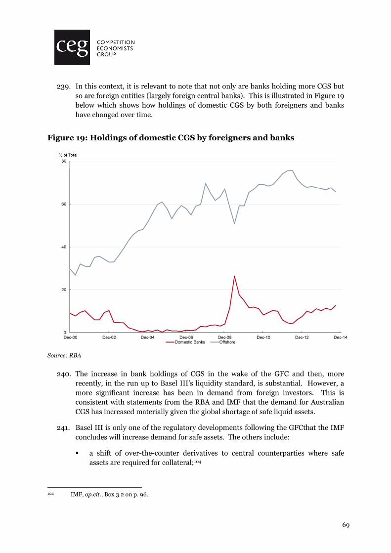
69

239. In this context, it is relevant to note that not only are banks holding more CGS but so are foreign entities (largely foreign central banks). This is illustrated in Figure 19 below which shows how holdings of domestic CGS by both foreigners and banks have changed over time.

Figure 19: Holdings of domestic CGS by foreigners and banks

Source: RBA

240. The increase in bank holdings of CGS in the wake of the GFC and then, more recently, in the run up to Basel III’s liquidity standard, is substantial. However, a more significant increase has been in demand from foreign investors. This is consistent with statements from the RBA and IMF that the demand for Australian CGS has increased materially given the global shortage of safe liquid assets.

241. Basel III is only one of the regulatory developments following the GFCthat the IMF concludes will increase demand for safe assets. The others include:

� a shift of over-the-counter derivatives to central counterparties where safe assets are required for collateral;104

104 IMF, op.cit., Box 3.2 on p. 96.

70

� limits on the reuse of collateral and the resulting reduction in the ‘velocity’ of collateral; 105 and

� higher risk weights in banking regulation for the holding of downgraded sovereign debt. 106

A.3.1 IMF summary

242. The following table is the IMF’s summary of the influences on the global supply and demand for safe assets. It summarises the reasons why the IMF believes:

The price of assets regarded as safe is on the rise, with supply dwindling

and demand rising amid uncertainty in financial markets, regulatory

reforms, and increased demand from central banks in advanced

economies.

…

While the “price of safety” will inevitably rise, a smooth adjustment

process can be ensured if policymakers are aware of their actions and

their potential consequences. 107

105 IMF, op.cit., see section “The Role of Safe Assets as Collateral, beginning on p. 96.

106 IMF, op.cit., see Box 3.3 on p. 97.

107 See IMF summary at: http://www.imf.org/external/pubs/ft/survey/so/2012/POL041112A.htm.

71

Table 11: IMF Table 3.3 (reproduced)

estimating the cost of equity, equity beta and mrp energy - 7.03 ceg... · estimating the cost of...

Documents