Transportation Research Part C 19 (2011) 1319–1325

Contents lists available at ScienceDirect

Transportation Research Part C

journal homepage: www.elsevier .com/locate / t rc

Estimating percent-time-spent-following on two-lane rural highways

Moshe Cohen a,⇑, Abishai Polus b

a Department of Industrial Engineering, Jerusalem College of Engineering, Schreibau Street, Jerusalem, Israelb Department of Civil and Environmental Engineering, Technion, Haifa 32000, Israel

a r t i c l e i n f o

Article history:Received 8 February 2010Received in revised form 13 March 2011Accepted 14 March 2011

Keywords:HighwaysRuralTwo-lanePTSFQueuing

0968-090X/$ - see front matter � 2011 Elsevier Ltddoi:10.1016/j.trc.2011.03.001

⇑ Corresponding author.E-mail addresses: bani@jce.ac.il (M. Cohen), polu

a b s t r a c t

This study concentrated on estimating the percent-time-spent-following (PTSF) on two-lane highways. This measure is a key estimate of level-of-service in traffic engineeringapplications. Its evaluation to date has been based on simulations that yielded over-estimated values. The present study shows how to estimate this variable from easilyobtained field data based on queuing theory. The estimates accord with opinions on yield-ing significantly lower values of PTSF that are expressed in the relevant traffic literature. Animproved relationship between PTSF and two-way flow is provided by fitting the newestimates by means of the least-squares method.

� 2011 Elsevier Ltd. All rights reserved.

1. Introduction

The level-of-service concept is commonly accepted in traffic engineering as a way to evaluate the quality and character-istics of flow on various facilities. For example, it is needed for decision-making on adding lanes, re-aligning highways andconducting safety analyses. This paper shows that utilizing relatively simple operations research methodologies may con-tribute directly to advancing important traffic engineering issues that have not previously been explored.

One of the recommended measures of the level-of-service of two-lane rural highways, according to the leading manual oftraffic analysis, the Highway Capacity Manual (HCM, 2000), is the proportion of time that fast vehicles travel in platoons be-hind slow vehicles. This proportion is typically measured by the Percentage of Time Spent Following (PTSF). In reality, it israther difficult to measure PTSF because of the complexity of collecting data for fast-traveling vehicles that follow slowervehicles. This means that direct measurement, which would also necessitate the use of complicated equipment would beprohibitively expensive, if not practically impossible, to make. An alternative would be to calculate PTSF from simulationruns; however, this approach has disadvantages, mainly because it requires assumptions regarding traffic characteristics,particularly the behavior of drivers in passing maneuvers. Previous studies have not provided other alternative analyticalapproaches for calculating PTSF values. The present research offers a theoretical model to determine PTSF values for differentflow conditions from readily available and easily observed traffic data. The new model provides values that are significantlylower than the HCM model, which is known to be overestimated (e.g., Harwood et al., 2003; Luttinen, 2001).

A few assumptions must be made to arrive at an analytical model to estimate PTSF. Although these simplifying assump-tions are not often fulfilled, they are fairly close to reality in some conditions. Without any assumptions, it becomes impos-sible to solve the model analytically; the assumptions in this work are necessary to derive a theoretical formula whosearguments are easily measurable quantities. Furthermore, it will be shown that the results of the model’s predictions of PTSFprovide values that are lower than the HCM values.

. All rights reserved.

s@technion.ac.il (A. Polus).

1320 M. Cohen, A. Polus / Transportation Research Part C 19 (2011) 1319–1325

2. Background

Previous studies that have dealt with estimating PTSF include the following: The Highway Capacity Manual (HCM, 2000,and previous editions) uses this variable as the main measure of the level-of-service of two-lane highways; the model pro-vided is based on simulation runs with the TWOPAS model (Dixon et al., 2003). Several studies (e.g., Harwood et al., 2003;Luttinen, 2001) suggested that the HCM values for PTSF were overestimated. A recent study (Al-Kaisy and Durbin (2007) alsosuggested that the HCM values of PTSF are overestimated and proposed a proxy measure of ‘‘percent following’’ (PF), whichis an estimate of the percentage of fast vehicles trapped in platoons at a specific location. However, the proposed measure isfor a static observer; it is not for the time-spent in platoons but rather for the number of vehicles in platoons. A previousstudy by the present authors (Polus and Cohen, 2009) suggested using PTSF as one of the potential measures of level-of-service, giving an estimate of its value as a function of the two-way flow on two-lane highways and based on easilyobservable quantities. That study focused mainly on a comparison of several measures of level-of-service and did not givea detailed explanation of the assumptions and the PTSF model’s details. Additionally, it was based on only 30 data points.Since then, significant additional data were collected and analyzed. Additionally, 71 new data points (in addition to the pre-vious 30) were added. Each of the 101 data point represents 1-h of one-way traffic. The current paper focuses on the detailsand assumptions and various conditions for estimating PTSF.

3. Elements of the model

The following symbols are used in the paper:

Symbol

Fast vehicle NumSlow vehicle

Fig. 1. Schematic diagram of one direction of a t

Meaning

h

headway �h average headway L average number of fast vehicles behind a slow vehicle N number of headways between two platoons N average number of headways between two platoons Q number of headways inside a platoon Q average number of headways inside a platoon s average speed of fast vehicles u average speed of slow vehicles V flow, average number of passenger-car equivalents per unit time W average time between joining a platoon and passing the first vehicle h average travel time between two platoons k arrival rate at the back of a moving queue p probability that a slow vehicle has no following platoon q traffic intensity, a parameter of the geometric distribution

Three assumptions were made during the development of the model: First, the speeds of fast and slow vehicles are assumedto be constant, denoted by s and u, respectively. Second, the flow of traffic is along an infinite homogeneous section, withoutany entrances or exists and with similar geometry. Third, the flow operates in a steady-state condition.

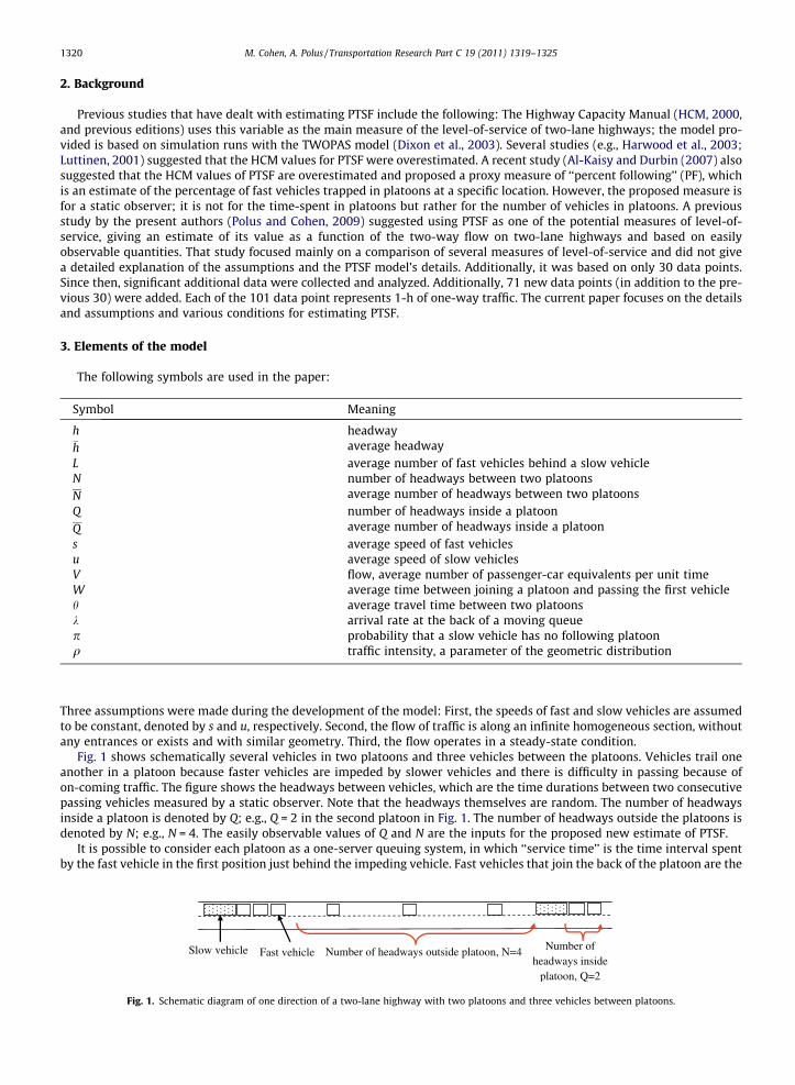
Fig. 1 shows schematically several vehicles in two platoons and three vehicles between the platoons. Vehicles trail oneanother in a platoon because faster vehicles are impeded by slower vehicles and there is difficulty in passing because ofon-coming traffic. The figure shows the headways between vehicles, which are the time durations between two consecutivepassing vehicles measured by a static observer. Note that the headways themselves are random. The number of headwaysinside a platoon is denoted by Q; e.g., Q = 2 in the second platoon in Fig. 1. The number of headways outside the platoons isdenoted by N; e.g., N = 4. The easily observable values of Q and N are the inputs for the proposed new estimate of PTSF.

It is possible to consider each platoon as a one-server queuing system, in which ‘‘service time’’ is the time interval spentby the fast vehicle in the first position just behind the impeding vehicle. Fast vehicles that join the back of the platoon are the

ber of headways outside platoon, N=4 Number of headways inside

platoon, Q=2

wo-lane highway with two platoons and three vehicles between platoons.

u s

s•h

u•τ

At time t:

At time (t+τ):

s•τ

Slow vehicle Fast vehicle

Observer.

Fig. 2. Two snapshots of a platoon and a joining fast vehicle.

M. Cohen, A. Polus / Transportation Research Part C 19 (2011) 1319–1325 1321

‘‘customers’’ in the system. Note that the inter-arrival times of fast vehicles reaching the platoon, as well as the ‘‘servicetime,’’ are stochastic. Note also that there must be some time when the queue is empty (i.e., a slow vehicle without fast vehi-cles behind it in a platoon) in order that a steady-state flow be maintained without diverging queues; this is assumed in thispaper. It follows, therefore, that the mean ‘‘service time’’ should not be greater than the mean inter-arrival time, as thiswould cause a queue to bring about an infinite queue in the long term. The influence of the opposing traffic is implicitly re-garded, because it is reflected by the passing rate. Therefore, if the opposing traffic is heavier, the ‘‘service time’’ is longer andobserved queue lengths are also longer, since it is more difficult to perform a passing maneuver. Hence, the observations of asingle lane include an implicit impact of the opposing flow.

The inter-arrival times of the fast vehicles at the back of the queue are not the same as the headways between vehicles asobserved by a static observer. The situation is schematically shown in Fig. 2, in which the last vehicle of the platoon shownpassed the static observer at time t and a following fast vehicle joins the platoon at time t + s.

The notation h represents the statically observed headway between the last vehicle in the platoon and the following fastvehicle as seen by the stationary observer. The speeds of the slow and the fast vehicles are also noted on Fig. 2: u and s,respectively. Therefore, the distance between the fast vehicle at time t and the static observer is s � h. The distance betweenthe fast vehicle at time t until it joins the platoon at time (t + s) is s � s. During the time s, the platoon traverses the distanceu � s. It follows that the inter-arrival times between fast vehicles at the back-end of the platoon is given by:

ss� u

� h ð1Þ

4. Data and analysis

Data on headways between vehicles were collected on 30 two-lane highways at different time intervals, typically in andaround the peak hour. The data were then segregated into 101 periods of 1 h each; for each highway, the peak hour itself wasselected first and then the remaining data were sliced into additional periods of 1-h each. The headway measurements wereconducted by a static observer at the road-side. Note that the required data can be collected easily and cheaply by simpledetectors. A typical portion of a file with data for Highway 75 East is shown in Fig. 3. The observed data consisted of one-way volumes up to approximately 1200 vph.

It is commonly accepted in Traffic Engineering (HCM, 2000) that if the headway between two consecutive vehicles is lessthan 3 s., they belong to the same platoon. According to this definition and the data available, such as shown in Fig. 3, it is easyfor the stationary observer to calculate the headways outside the platoons from the arrival times. A typical headway outside aplatoon is denoted by h; see Fig. 2. It is easy to calculate the number of headways inside and outside the platoons; Q and N,respectively. An example of Q and N, is shown in Fig. 1 and an example of the data for their calculation is shown in Fig. 3.

Geometric distributions were fitted to all 101 hourly data sets of headways inside platoons (Q). A typical histogram withthis fit for the data from Highway 75 East is shown in Fig. 4.

The probability function of the geometric distribution is given in Eq. (2) as:

ProbfQ ¼ ig ¼ ð1� qÞ � qði�1Þ i ¼ 1;2;3; . . . ð2Þ

where Q is the number of headways inside platoons and q is estimated from the data and represents the traffic intensity. Theestimate of q from the data is as follows:

q ¼ 1� 1Q

ð3Þ

Fig. 3. Example of a file containing part of headway data for Highway 75 East.

Fig. 4. Histogram of Q vs. expected value, assuming geometric distribution.

1322 M. Cohen, A. Polus / Transportation Research Part C 19 (2011) 1319–1325

The null hypothesis that Q is geometrically distributed may be tested by the chi-square test of ‘‘goodness of fit.’’ If thep-value is above some threshold (say, 5% = probability of error of first kind), the null hypothesis of a satisfactory fit cannotbe rejected. For 96 of the 101 samples, the p-values were indeed above 0.05. By the very meaning of the error of the first kind,five cases of the 101 on the average may produce lower p-values than 0.05, given that the null hypothesis is true. Therefore,the null hypothesis is not rejected for any data sets. In the following development it will be assumed that Q, the number ofheadways inside platoons, is geometrically distributed.

5. Derivation of PTSF estimates

The percent-time-spent-following (PTSF) is used as a measure of the level-of-service of the flow on two-lane highways. Itis simply the ratio between the time spent in platoons and the total travel time, expressed in percentages. The road is com-posed of groups of vehicles, some traveling in platoons and some traveling freely, in-between platoons. For the analysis, it ispossible to select a typical sequence of vehicles in an average platoon, followed by an average number of freely moving fastvehicles, up to the next platoon. This is shown in Fig. 5. Note that it is possible that no free-flowing vehicles may be locatedbetween two platoons. In such a case, the number of gaps between the platoons is 1. This possibility is included when cal-culating the average number of gaps between platoons.

Platoon Average Platoon Average Free Flowing Vehicles between Platoons

Platoon

Average Sequence of Vehicles for Analysis

Fig. 5. Definition of average sequence of vehicles for analysis.

M. Cohen, A. Polus / Transportation Research Part C 19 (2011) 1319–1325 1323

In this analysis, a ‘‘system’’ consists of a slow-moving impeding vehicle and a possible following fast vehicle or vehiclesbehind it, forming a platoon. The system would be ‘‘empty’’ if a slow-moving vehicle does not have fast vehicles immediatelybehind it. Note that single slow-moving vehicles representing such a system cannot be observed if only the number of vehi-cles inside and outside platoons is counted. The ‘‘service’’ is the time that a fast vehicle spends while waiting for an appro-priate gap in order to pass, including the time needed to complete the pass. A queue consists of the fast vehicles behind aslow-moving vehicle; note that this number is equal to the number of gaps inside a platoon; see Fig. 5.

Following Pollatschek and Polus (2005), we assumed that the inter-arrival times between vehicles at the back of a platoonand the ‘‘service times’’ are random. The assumed queuing model is M/M/1; justification is as follows: The number of trailingvehicles in platoons was geometrically distributed as shown in Fig. 4 for one sample data set. The geometric assumptioncould not be statistically rejected after the analysis of all our data sets. The geometric distribution strongly suggests anM/M/1 queuing model, as the queue lengths in this model are distributed geometrically. Other possibilities are to apply otherqueuing systems with the following two requirements: it should be a 1-server system, and the number of ‘‘customers’’ (vehi-cles) in the system should be distributed geometrically. An M/M/1 system was selected because it is the simplest system thatfits the field findings (Occam’s razor principle).

The following variables were denoted:

� W = average time in system, average time of traveling in platoon from moment of joining the back of the platoon till themoment of the start of the passing maneuver;� h = average travel time between platoons.

Then PTSF is given by:

PTSF ¼ 100W

hþWð4Þ

Eq. (4) assumes that passing opportunities are not impeded by no-passing zones; therefore, no-passing zones are neglectedin our model. The average number of ‘‘customers in the system’’ is not the average observed Q, (average number of headwaysinside platoons), denoted by Q , because Q is counted only when the queue has ‘‘customers.’’ Unfortunately, with the avail-able data, as shown in Fig. 3, it is impossible to identify the slow vehicles without an attached platoon. These vehicles, whichcan create a platoon at a later moment, will be termed ‘‘unobserved’’ slow vehicles. In queuing theory, this is equivalent to asystem without customers; i.e., an ‘‘empty system.’’ However, there is the possibility of assuming the probability of an emptysystem. This probability is denoted by p. Therefore, Eq. (2) becomes:

ProbfQ ¼ ig ¼p i ¼ 0ð1� pÞ � ð1� qÞ � qi�1 i > 0

�ð5Þ

The value of p could be either zero (no cases of slow vehicles without fast vehicles behind them) or derived from anextension of the geometric distribution toward zero. The latter implies that p = 1 � q. If p = 0, then L, the average numberof ‘‘customers in the system’’ (average of number of fast cars in a platoon; i.e., number of headways in a platoon) is Q . Ifp = 1 � q, then Eq. (5) is the usual geometric distribution, and L is given as in Eq. (6) after using the relationship shownin Eq. (3) and simplifying:

L ¼ q � Q ¼ Q � 1 ð6Þ

However, if p is between 0 and 1 � q – say it has the same probability as the probability of observing an average platoonof two cars (i = 2 in Eq. (2)) –then it can be shown, after using the relationship shown in Eq. (3) and simplifying, that:

L ¼ Q 2 þ 1� Q

Qð7Þ

To obtain the average time that a fast vehicle spends in a platoon, W, from the average number of customers in the sys-tem, L, it is possible to use Little’s law (Asmussen, 2003, Theorem 4.1, p. 276). To do so requires the rate of arrivals at the backof the platoon, or the arrival intensity. This intensity is a reciprocate of the average headway between the end of the platoon

1324 M. Cohen, A. Polus / Transportation Research Part C 19 (2011) 1319–1325

and the fast vehicle behind it. As previously discussed, the expected value of this headway is estimated to be the averageheadway between platoons, denoted by �h. Hence, the arrival intensity, k, for a static observer is 1

�h; from Eq. (1) it follows that

the arrival intensity at the back of a moving queue is given by Eq. (8) as:

k ¼ s� u

s � �hð8Þ

where s and u are the speeds of the fast and slow vehicles, respectively.From Little’s theorem, it follows that the average timespent in the system (platoon), W, is given as in Eq. (9):

W ¼ Lk¼

Q �s��hs�u if p ¼ 0ðQ�1Þ�s��h

s�u if p ¼ 1� qQ2 �s��h

ðQ�1Þ�ðs�uÞif p ¼ ProbfQ ¼ 2g

8>>><>>>:

ð9Þ

The estimate of the average travel time between platoons, h, will be �h multiplied by the number of headways between fastvehicles that travel freely between platoons, N � �h, corrected for a moving platoon (note Fig. 1) by using Eq. (1). This is shownin Eq. (10):

h ¼ N � �h � ss� u

ð10Þ

In this development, the ‘‘unobserved’’ slow vehicles that may be present among free-flowing vehicles between platoonswere taken into account by including p (the probability that there is no trailing fast vehicle following a slow vehicle) in Eq.(9).

When Eqs. (9) and (10) are substituted into Eq. (4), the results, seen in Eq. (11), are obtained for PTSF, the percent-time-spent-following:

PTSF ¼

100 � QNþQ

if p ¼ 0

100 � Q�1NþQ�1

if p ¼ 1� q

100 � Q2=Q�1NþQ2=Q�1

if p ¼ ProbfQ ¼ 2g

8>>>><>>>>:

ð11Þ

6. PTSF as a function of flow

For traffic engineering purposes, there is often need to estimate the value of PTSF as a function of flow. The flow isobtained from the counted number of vehicles and converted to a number of passenger-car equivalents per hour in eachdirection. The flow assumes that the busiest 15-min. period within the peak hour lasts for the full peak hour. It is necessaryto convert the one-way volume to a two-way flow because it is desirable to compare the new development to the commonlyused values of HCM (2000).

Fig. 6. Proposed relationship between two-way flow and percent-time-spent-following and a comparison to HCM values.

M. Cohen, A. Polus / Transportation Research Part C 19 (2011) 1319–1325 1325

For the 101 available data sets, the volume is the number of rows (note Fig. 3); the conversion to a two-way flow isapproximated by multiplying by 2 and dividing by 0.8 and 0.963, which represent the within-peak-hour distribution andthe conversion into equivalent number of cars, respectively. These values are average values obtained from the collected datafor the 101 data sets.

In a previous publication, Polus and Cohen (2009) did not present a detailed description of the assumptions and devel-opments needed to arrive at the three forms of Eq. (11). They gave only the middle expression for PTSF from Eq. (11) byextrapolating the geometric distribution for a value of zero trailing vehicles in the ‘‘unobserved’’ platoons. The probabilityof this happening is p = 1 – q.

Fig. 6 presents the proposed relationship between the two-way flow on two-lane highways and the percent-time-spentfollowing (PTSF), along with a comparison to HCM (2000) values. The data points were obtained from 30 two-lane highwaysand 101 data sets of 1-h period each; note Fig. 3. A conversion of the counted vehicles to a two-lane flow was conducted inorder to be able to compare the estimates of PTSF to the proposed HCM values. HCM uses the functional form100 � [1 � exp(�aV)], where V is the two-way flow and a is a constant. The same functional form was used for a least-squares fitting of the curve to the data points. The coefficient a was found to be 0.0005.

The new PTSF values are shown for two cases of p: The upper line, closer to the HCM (2000) model, represents the lowestpossible value of p (p = 0); the triangular markers represent the 101 data points for which this line is fitted. The lower dashedline represents the case in which p = (1 � q), which is assumed to be the largest possible value of p; its 101 data points arethe small ‘‘plus’’ markers. All other cases of p are between these two values, including the third line in Eq. (11). The true PTSFvalue is somewhere between these two ‘‘extreme’’ lines, but probably closer to the HCM model. Thus, regardless of the exactvalue of p, HCM’s PTSF values are higher than those found in the proposed model, independently of the value of p.

It may be noticed that the proposed model is significantly lower than the HCM values, and thus it supports the opinionsexpressed in previous studies (e.g., Harwood et al., 2003; Luttinen, 2001; Al-Kaisy and Durbin, 2007).

7. Summary and conclusions

This study focused on the development of a new method estimating the PTSF measure of level-of-service from easilyobtained observations. The estimation and the new method are based on field data and the assumption of relevance ofthe M/M/1 queuing model; the relative low volumes and the exponential distribution of headways in this case make themodel relevant. Each data set leads to the PTSF estimation for the observed volume, and consequently a model between PTSFand flow was developed (note Fig. 6). If field data is available to a planning agency, it is best to use the proposed method andto estimate the PTSF directly for a specific site. However, if the required data is not available, the model to predict PTSF fromthe flow may be used in planning analysis.

The two extreme cases of p occurs when p = 0 and when p = 1 � q. The two lower lines in Fig. 6 correspond to these twocases. The true PTSF value probably lies somewhere between the two lines, and probably closer to the HCM model. The mainconclusion is that regardless of the exact value of p, the HCM’s PTSF values are most likely overestimated. This conditioncould be remedied by recalculating PTSF based on simple measureable parameters of the number of vehicles found betweenplatoons and inside platoons. It is suggested that for planning purposes, use be made of the value closest to the HCM (2000)values; i.e., of p = 0 (hence, the first row of Eq. (11)).

The level-of-service concept and its evaluation, is a key consideration in various traffic engineering analyses and appli-cations. For example, it is needed for evaluating the quality of flow on different facilities, for making a decision on addinglanes, for re-aligning highways, etc. The importance of the developments proposed in this paper lies in the fact that byutilizing relatively simple operations research methods, it is possible to advance the state-of-the art in other engineeringdisciplines, such as traffic engineering. The proposed method of estimating PTSF combines theory with field data, a combi-nation, it is shown, that can be a powerful tool to provide reasonable estimations of measures that are otherwise very dif-ficult to estimate.

References

Al-Kaisy, A., Durbin, C., 2007. Estimating percent time spent following on two-lane highways: field evaluation of new methodologies. In: TransportationResearch Board 86th Annual Meeting (CD-ROM).

Asmussen, S., 2003. Applied Probability and Queues, second ed. Springer, New York.Dixon, M.P., Haderlie, S., Sarepalli, A.S.K., 2003. Using TWOPAS Simulation Model to Provide Design and Operations Information on the Performance of

Idaho’s Two-Lane Highways. National Institute for Advanced Transportation Technology, University of Idaho, Final Report, KLK 468.Harwood, D.W., Potts, I.B., Bauer, K.M., Bonneson, J., Elefteriadou, L., 2003. Two-Lane Road Analysis Methodology in the Highway Capacity Manual. National

Cooperative Highway Research Program, NCHRP Project 20-7. Transportation Research Board, National Research Council, Washington, DC.Highway Capacity Manual (HCM), 2000. Transportation Research Board, National Research Council, Washington, DC.Luttinen, R.T., 2001. Percent time-spent-following as performance measure for two-lane highways. Transportation Research Record 1776, 52–59.Pollatschek, M.A., Polus, A., 2005. Modeling impatience of drivers in passing maneuvers. In: Mahmassani, H.S. (Ed.), Transportation and Traffic Theory

(ISTTT16). Elsevier Science & Pergamon Pub., pp. 267–280.Polus, A., Cohen, M.A., 2009. Theoretical and empirical relationships for the quality of flow and for a new level-of-service on two-lane highways. Journal of

Transportation Engineering, ASCE 135 (6), 380–385.