Estimating Domestic U.S. Airline

Cost of Delay based on European Model

Abdul Qadar Kara, John Ferguson, Karla Hoffman, Lance Sherry

George Mason University Fairfax, VA, USA

akara;jfergus3;khoffman;lsherry@gmu.edu

Abstract— In this paper, we detail a method for calculating the

cost of delays to an airline. The approach extends a EU report

that calculated delays for three alternative scenarios (low cost,

baseline costs and high costs) and for short delays (under 15

minutes) and long delays (over 65 minutes). Our extension to this

report determines the factors that make up the multipliers

presented in that report. We next apply the individual cost factor

delays to US data. The approach allows one to update the cost

whenever any of the factors (crew, fuel, maintenance, ground

costs) change. It considers the size of the aircraft when making

such calculations, both from the perspective of fuel burn and

passenger costs. Our validation methodology evaluates how close

our data come to that presented in their report when a

conversion is made from dollars to Euros and applies 2003 cost

data. Data for Philadelphia airport (PHL) is displayed as a case

study to show current delay costs.

Keywords-component; airline delay costs; airline delays;

economic modeling of airlines;

I. INTRODUCTION

The airline industry moves millions of passengers and tons of cargo annually. The Schumer report estimated that in 2007, airport delays cost about 40.7 billion dollars to the economy [1]. Disruptions in one part of the airspace impact the entire network as delays propagate. It is estimated that almost 50% of the entire airspace delays are caused by delays that originate at the New York/New Jersey/ Pennsylvania airports. We begin this study by considering only the direct costs to the airlines of such delays. Future work will examine the network impact as well as the resulting economics costs to the various regions and other industries. In general a flight can be delayed due to several reasons, mainly:

- Mechanical problems with the aircraft.

- Schedule disruption due to bad weather or air traffic

management initiatives (Ground Delay Programs

(GDPs) or Air Flow Programs (AFPs)).

- Misaligned crew/ aircraft due to previous delayed

flight

Weather is a major cause of delay as it reduces the capacity of both the airspace and the runways. Based on weather forecasts, air traffic management estimates the resulting reduction in capacity within various segments of the airspace and at a variety of airports. It announces Ground Delay Programs (GDPs) that hold aircraft at the departing airport, in order to have the flying aircraft better match the capacity of the system. Holding at a gate is both cheaper and safer than airborne holds, and allows the system to be better managed. Finally, the delays already described induce future delays in the system, because the aircraft or crews may not arrive at their next assignment on time. Even when the crew does arrive, they may not be able to work another flight because they have exceeded their allowable working hours. In this paper, we focus on the final report prepared by the Performance Review Unit, Eurocontrol in 2004[2]. This EU report describes a methodology and presents results detailing the cost to airlines of delays during various segments of a trip. The costs are divided into short delays (less than 15 minute) and long delays (greater than 65). The report provides the resultant multiplier (Euros per minute) for any such segment. The types of delays considered include gate delay, access to runway delay (both taxi in and out delays), on routes delays, and landing delays (circling or longer flight paths to overcome congestion while approaching the airport). The data used in the study consisted of data collected from European airlines, air traffic management as well as interviews and surveys conducted by the research team. This paper is organized as follows. Section II describes the EU report, Section III provides our methodology for determining the cost components and multipliers that make up the final multipliers used in the Eurocontrol report and describe our validation of the new model on European data from the period of the EU report. In Section IV, we apply our methodology to 8 weather days at Philadelphia as a case study and show the resulting delay costs for these flights. Section V provides conclusions and Section VI points out the future research.

II. PERFORMANCE REVIEW UNIT REPORT (EU REPORT)

The EU report specifies that delays incurred can be of two types: tactical delay and strategic delay. The report makes the distinction between tactical delays (delays encountered that

This research was partially funded under NASA grant NNX09AB20A.)

are greater than the announced schedule, i.e. delays above the anticipated padding of the schedule) and strategic delays (i.e. the delay relative to an unpadded schedule). Both US and European airlines increase the arrival time over unimpeded time so that they can report “on time” performance even when the system is over-capacitated. Another distinction that the report makes is between gate-to-gate (or single flight) delays

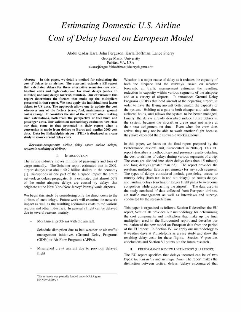
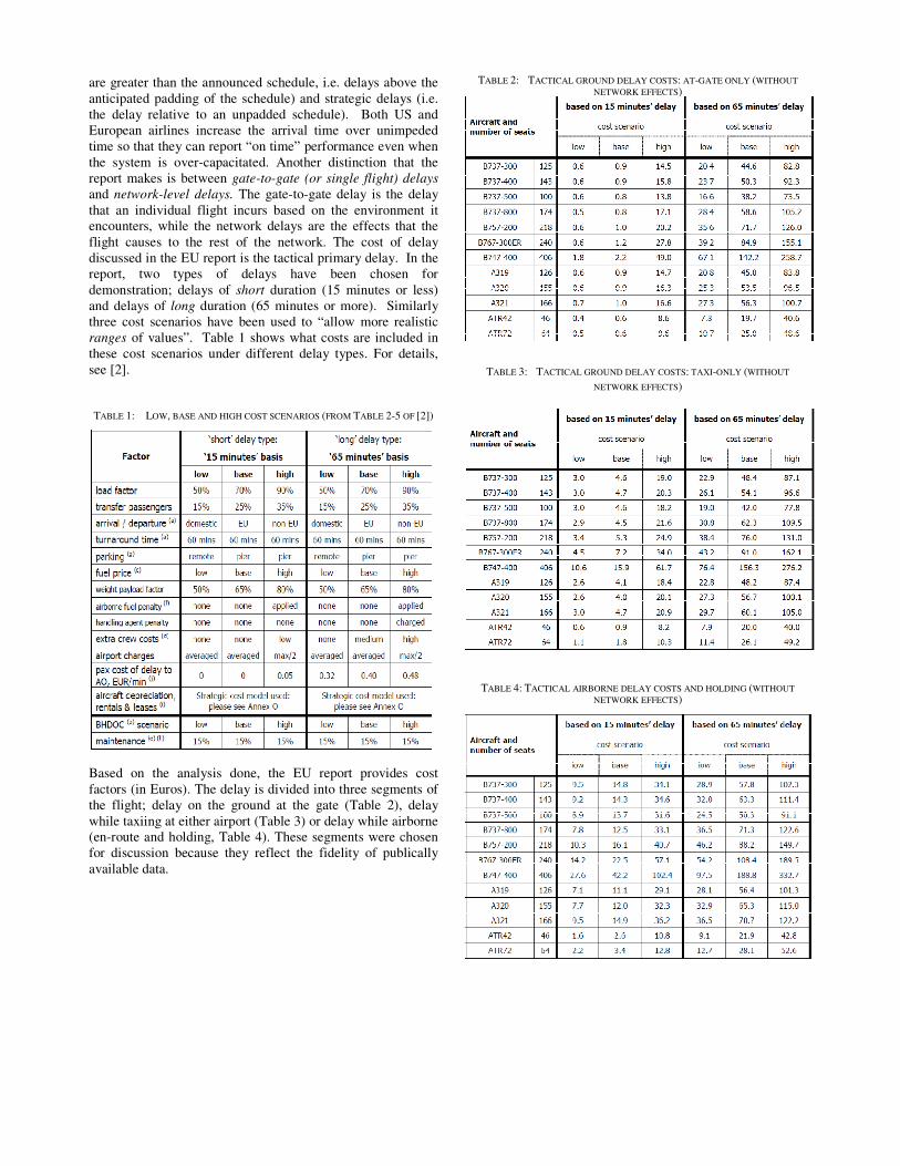
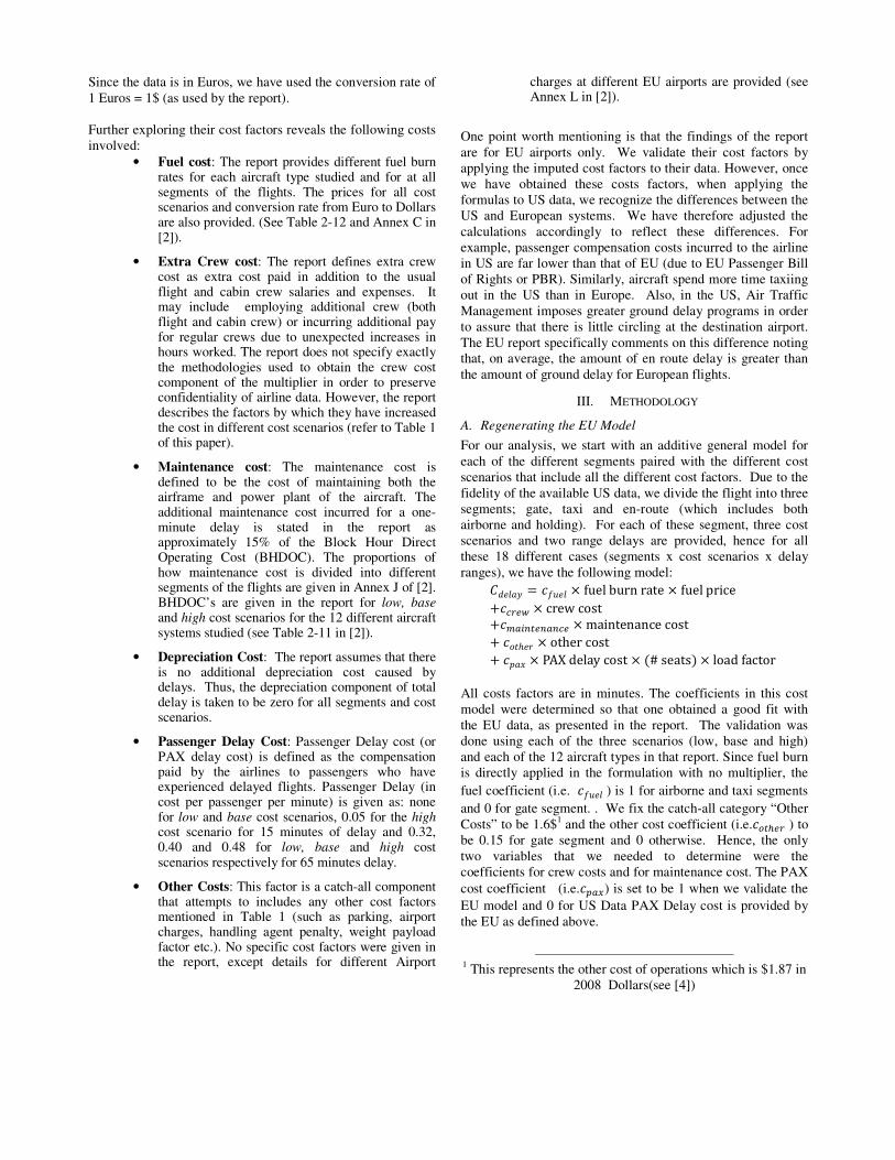
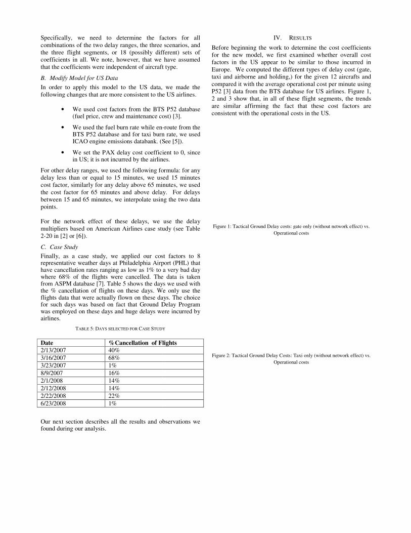
and network-level delays. The gate-to-gate delay is the delay that an individual flight incurs based on the environment it encounters, while the network delays are the effects that the flight causes to the rest of the network. The cost of delay discussed in the EU report is the tactical primary delay. In the report, two types of delays have been chosen for demonstration; delays of short duration (15 minutes or less) and delays of long duration (65 minutes or more). Similarly three cost scenarios have been used to “allow more realistic ranges of values”. Table 1 shows what costs are included in these cost scenarios under different delay types. For details, see [2].

TABLE 1: LOW, BASE AND HIGH COST SCENARIOS (FROM TABLE 2-5 OF [2])

Based on the analysis done, the EU report provides cost factors (in Euros). The delay is divided into three segments of the flight; delay on the ground at the gate (Table 2), delay while taxiing at either airport (Table 3) or delay while airborne (en-route and holding, Table 4). These segments were chosen for discussion because they reflect the fidelity of publically available data.

TABLE 2: TACTICAL GROUND DELAY COSTS: AT-GATE ONLY (WITHOUT

NETWORK EFFECTS)

TABLE 3: TACTICAL GROUND DELAY COSTS: TAXI-ONLY (WITHOUT

NETWORK EFFECTS)

TABLE 4: TACTICAL AIRBORNE DELAY COSTS AND HOLDING (WITHOUT

NETWORK EFFECTS)

Since the data is in Euros, we have used the conversion rate of 1 Euros = 1$ (as used by the report). Further exploring their cost factors reveals the following costs involved:

• Fuel cost: The report provides different fuel burn rates for each aircraft type studied and for at all segments of the flights. The prices for all cost scenarios and conversion rate from Euro to Dollars are also provided. (See Table 2-12 and Annex C in [2]).

• Extra Crew cost: The report defines extra crew cost as extra cost paid in addition to the usual flight and cabin crew salaries and expenses. It may include employing additional crew (both flight and cabin crew) or incurring additional pay for regular crews due to unexpected increases in hours worked. The report does not specify exactly the methodologies used to obtain the crew cost component of the multiplier in order to preserve confidentiality of airline data. However, the report describes the factors by which they have increased the cost in different cost scenarios (refer to Table 1 of this paper).

• Maintenance cost: The maintenance cost is defined to be the cost of maintaining both the airframe and power plant of the aircraft. The additional maintenance cost incurred for a one-minute delay is stated in the report as approximately 15% of the Block Hour Direct Operating Cost (BHDOC). The proportions of how maintenance cost is divided into different segments of the flights are given in Annex J of [2]. BHDOC’s are given in the report for low, base and high cost scenarios for the 12 different aircraft systems studied (see Table 2-11 in [2]).

• Depreciation Cost: The report assumes that there is no additional depreciation cost caused by delays. Thus, the depreciation component of total delay is taken to be zero for all segments and cost scenarios.

• Passenger Delay Cost: Passenger Delay cost (or PAX delay cost) is defined as the compensation paid by the airlines to passengers who have experienced delayed flights. Passenger Delay (in cost per passenger per minute) is given as: none for low and base cost scenarios, 0.05 for the high cost scenario for 15 minutes of delay and 0.32, 0.40 and 0.48 for low, base and high cost scenarios respectively for 65 minutes delay.

• Other Costs: This factor is a catch-all component that attempts to includes any other cost factors mentioned in Table 1 (such as parking, airport charges, handling agent penalty, weight payload factor etc.). No specific cost factors were given in the report, except details for different Airport

charges at different EU airports are provided (see Annex L in [2]).

One point worth mentioning is that the findings of the report are for EU airports only. We validate their cost factors by applying the imputed cost factors to their data. However, once we have obtained these costs factors, when applying the formulas to US data, we recognize the differences between the US and European systems. We have therefore adjusted the calculations accordingly to reflect these differences. For example, passenger compensation costs incurred to the airline in US are far lower than that of EU (due to EU Passenger Bill of Rights or PBR). Similarly, aircraft spend more time taxiing out in the US than in Europe. Also, in the US, Air Traffic Management imposes greater ground delay programs in order to assure that there is little circling at the destination airport. The EU report specifically comments on this difference noting that, on average, the amount of en route delay is greater than the amount of ground delay for European flights.

III. METHODOLOGY

A. Regenerating the EU Model

For our analysis, we start with an additive general model for each of the different segments paired with the different cost scenarios that include all the different cost factors. Due to the fidelity of the available US data, we divide the flight into three segments; gate, taxi and en-route (which includes both airborne and holding). For each of these segment, three cost scenarios and two range delays are provided, hence for all these 18 different cases (segments x cost scenarios x delay ranges), we have the following model:

������ � ��� � fuel burn rate � fuel price

������ � crew cost

��!"#$%�$"$�� � maintenance cost

� �'()�* � other cost

� �,�- � PAX delay cost � 3# seats5 � load factor

All costs factors are in minutes. The coefficients in this cost model were determined so that one obtained a good fit with the EU data, as presented in the report. The validation was done using each of the three scenarios (low, base and high) and each of the 12 aircraft types in that report. Since fuel burn is directly applied in the formulation with no multiplier, the

fuel coefficient (i.e. ��� ) is 1 for airborne and taxi segments

and 0 for gate segment. . We fix the catch-all category “Other Costs” to be 1.6$1 and the other cost coefficient (i.e.�6%7�� ) to be 0.15 for gate segment and 0 otherwise. Hence, the only two variables that we needed to determine were the coefficients for crew costs and for maintenance cost. The PAX

cost coefficient (i.e.�8"9) is set to be 1 when we validate the

EU model and 0 for US Data PAX Delay cost is provided by the EU as defined above.

1 This represents the other cost of operations which is $1.87 in

2008 Dollars(see [4])

Specifically, we need to determine the factors for all combinations of the two delay ranges, the three scenarios, and the three flight segments, or 18 (possibly different) coefficients in all. We note, however, that we have assumed that the coefficients were independent of aircraft type.

B. Modify Model for US Data

In order to apply this model to the US data, we made the following changes that are more consistent to the US airlines.

• We used cost factors from the BTS P52 database (fuel price, crew and maintenance cost)

• We used the fuel burn rate while enBTS P52 database and for taxi burn rate, we used ICAO engine emissions databank. (See [

• We set the PAX delay cost coefficient to 0, in US; it is not incurred by the airlines

For other delay ranges, we used the following formula: for any delay less than or equal to 15 minutes, we used 15 minutes cost factor, similarly for any delay above 65 minutes, we used the cost factor for 65 minutes and above delaybetween 15 and 65 minutes, we interpolate using the two data points. For the network effect of these delays, we use the delay multipliers based on American Airlines case study (see Table 2-20 in [2] or [6]).

C. Case Study

Finally, as a case study, we applied our cost representative weather days at Philadelphia Airport (have cancellation rates ranging as low as 1% to a very bad day where 68% of the flights were cancelled. The data is from ASPM database [7]. Table 5 shows the days we used witthe % cancellation of flights on these days. We only use the flights data that were actually flown on these days. The choice for such days was based on fact that Ground Delay Program was employed on these days and huge delays were incurred by airlines.

TABLE 5: DAYS SELECTED FOR CASE STUDY

Date %Cancellation of Flights

2/13/2007 40%

3/16/2007 68%

3/23/2007 1%

8/9/2007 16%

2/1/2008 14%

2/12/2008 14%

2/22/2008 22%

6/23/2008 1%

Our next section describes all the results and observations we found during our analysis.

determine the factors for all combinations of the two delay ranges, the three scenarios, and

18 (possibly different) sets of . We note, however, that we have assumed

dependent of aircraft type.

In order to apply this model to the US data, we made the following changes that are more consistent to the US airlines.

We used cost factors from the BTS P52 database cost) [3].

We used the fuel burn rate while en-route from the BTS P52 database and for taxi burn rate, we used ICAO engine emissions databank. (See [5]).

coefficient to 0, since in US; it is not incurred by the airlines.

For other delay ranges, we used the following formula: for any delay less than or equal to 15 minutes, we used 15 minutes cost factor, similarly for any delay above 65 minutes, we used

delay. For delays using the two data

For the network effect of these delays, we use the delay multipliers based on American Airlines case study (see Table

we applied our cost factors to 8 Philadelphia Airport (PHL) that as low as 1% to a very bad day

The data is taken shows the days we used with

We only use the flights data that were actually flown on these days. The choice for such days was based on fact that Ground Delay Program was employed on these days and huge delays were incurred by

TUDY

of Flights

all the results and observations we

IV. RESULTS

Before beginning the work to determine the cost coefficients for the new model, we first examined whether overall cost factors in the US appear to be similar to those incurred in Europe. We computed the different types of delay cost (gatetaxi and airborne and holding,) for the given 12 aircraftscompared it with the average operational costP52 [3] data from the BTS database for US airlines2 and 3 show that, in all of these flight segmentsare similar affirming the fact that these cost factors are consistent with the operational costs in

Figure 1: Tactical Ground Delay costs: gate only (without network effect) vs.

Operational costs

Figure 2: Tactical Ground Delay Costs: Taxi only (without network effect) vs.

Operational costs

ESULTS

Before beginning the work to determine the cost coefficients for the new model, we first examined whether overall cost factors in the US appear to be similar to those incurred in

computed the different types of delay cost (gate, airborne and holding,) for the given 12 aircrafts and

compared it with the average operational cost per minute using for US airlines. Figure 1,

flight segments, the trends the fact that these cost factors are

consistent with the operational costs in the US.

: Tactical Ground Delay costs: gate only (without network effect) vs.

Operational costs

ts: Taxi only (without network effect) vs.

Operational costs

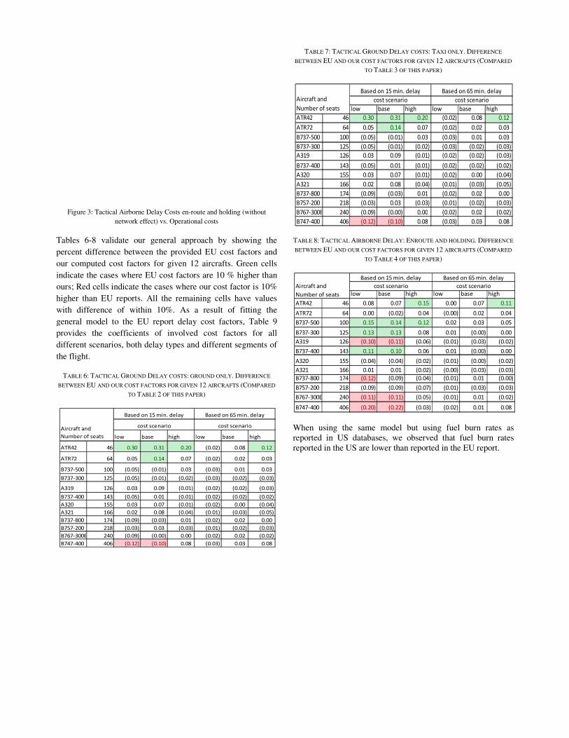
Figure 3: Tactical Airborne Delay Costs en-route and holding (without

network effect) vs. Operational costs

Tables 6-8 validate our general approach by showing the

percent difference between the provided EU cost factors and

our computed cost factors for given 12 aircrafts. Green cells

indicate the cases where EU cost factors are 10 % higher than

ours; Red cells indicate the cases where our cost factor is 10%

higher than EU reports. All the remaining cells have values

with difference of within 10%. As a result of fitting the

general model to the EU report delay cost factors, Table

provides the coefficients of involved cost factors for all

different scenarios, both delay types and different

the flight.

TABLE 6: TACTICAL GROUND DELAY COSTS: GROUND ONLY

BETWEEN EU AND OUR COST FACTORS FOR GIVEN 12 AIRCRAFTS

TO TABLE 2 OF THIS PAPER)

low base high low base

ATR42 46 0.30 0.31 0.20 (0.02)

ATR72 64 0.05 0.14 0.07 (0.02)

B737-500 100 (0.05) (0.01) 0.03 (0.03)

B737-300 125 (0.05) (0.01) (0.02) (0.03)

A319 126 0.03 0.09 (0.01) (0.02)

B737-400 143 (0.05) 0.01 (0.01) (0.02)

A320 155 0.03 0.07 (0.01) (0.02)

A321 166 0.02 0.08 (0.04) (0.01)

B737-800 174 (0.09) (0.03) 0.01 (0.02)

B757-200 218 (0.03) 0.03 (0.03) (0.01)

B767-300ER 240 (0.09) (0.00) 0.00 (0.02)

B747-400 406 (0.12) (0.10) 0.08 (0.03)

Aircraft and

Number of seats

Based on 15 min. delay Based on 65 min. delay

cost scenario cost scenario

route and holding (without

8 validate our general approach by showing the

he provided EU cost factors and

our computed cost factors for given 12 aircrafts. Green cells

indicate the cases where EU cost factors are 10 % higher than

ours; Red cells indicate the cases where our cost factor is 10%

ining cells have values

As a result of fitting the

general model to the EU report delay cost factors, Table 9

provides the coefficients of involved cost factors for all

different scenarios, both delay types and different segments of

GROUND ONLY. DIFFERENCE

AIRCRAFTS (COMPARED

TABLE 7: TACTICAL GROUND DELAY COSTS

BETWEEN EU AND OUR COST FACTORS FOR GIVEN

TO TABLE 3 OF THIS PAPER

TABLE 8: TACTICAL AIRBORNE DELAY: ENROUTE AND HOLDING

BETWEEN EU AND OUR COST FACTORS FOR GIVE

TO TABLE 4 OF THIS PAPER

When using the same model but using fuel burn rates as reported in US databases, we observed that fuel burn rates reported in the US are lower than reported

base high

0.08 0.12

0.02 0.03

0.01 0.03

(0.02) (0.03)

(0.02) (0.03)

(0.02) (0.02)

0.00 (0.04)

(0.03) (0.05)

0.02 0.00

(0.02) (0.03)

0.02 (0.02)

0.03 0.08

Based on 65 min. delay

cost scenario

low base high

ATR42 46 0.30 0.31 0.20

ATR72 64 0.05 0.14 0.07

B737-500 100 (0.05) (0.01) 0.03

B737-300 125 (0.05) (0.01) (0.02)

A319 126 0.03 0.09 (0.01)

B737-400 143 (0.05) 0.01 (0.01)

A320 155 0.03 0.07 (0.01)

A321 166 0.02 0.08 (0.04)

B737-800 174 (0.09) (0.03) 0.01

B757-200 218 (0.03) 0.03 (0.03)

B767-300ER 240 (0.09) (0.00) 0.00

B747-400 406 (0.12) (0.10) 0.08

Aircraft and

Number of seats

Based on 15 min. delay

cost scenario

low base high

ATR42 46 0.08 0.07 0.15

ATR72 64 0.00 (0.02) 0.04

B737-500 100 0.15 0.14 0.12

B737-300 125 0.13 0.13 0.08

A319 126 (0.10) (0.11) (0.06)

B737-400 143 0.11 0.10 0.06

A320 155 (0.04) (0.04) (0.02)

A321 166 0.01 0.01 (0.02)

B737-800 174 (0.12) (0.09) (0.04)

B757-200 218 (0.09) (0.09) (0.07)

B767-300ER 240 (0.11) (0.11) (0.05)

B747-400 406 (0.20) (0.22) (0.03)

Based on 15 min. delay

cost scenarioAircraft and

Number of seats

AY COSTS: TAXI ONLY. DIFFERENCE

FOR GIVEN 12 AIRCRAFTS (COMPARED

OF THIS PAPER)

NROUTE AND HOLDING. DIFFERENCE

FOR GIVEN 12 AIRCRAFTS (COMPARED

OF THIS PAPER)

but using fuel burn rates as we observed that fuel burn rates

reported in the EU report.

low base high

0.20 (0.02) 0.08 0.12

0.07 (0.02) 0.02 0.03

0.03 (0.03) 0.01 0.03

(0.02) (0.03) (0.02) (0.03)

(0.01) (0.02) (0.02) (0.03)

(0.01) (0.02) (0.02) (0.02)

(0.01) (0.02) 0.00 (0.04)

(0.04) (0.01) (0.03) (0.05)

0.01 (0.02) 0.02 0.00

(0.03) (0.01) (0.02) (0.03)

0.00 (0.02) 0.02 (0.02)

0.08 (0.03) 0.03 0.08

Based on 65 min. delay

cost scenario

low base high

0.15 0.00 0.07 0.11

0.04 (0.00) 0.02 0.04

0.12 0.02 0.03 0.05

0.08 0.01 (0.00) 0.00

(0.06) (0.01) (0.03) (0.02)

0.06 0.01 (0.00) 0.00

(0.02) (0.01) (0.00) (0.02)

(0.02) (0.00) (0.03) (0.03)

(0.04) (0.01) 0.01 (0.00)

(0.07) (0.01) (0.03) (0.03)

(0.05) (0.01) 0.01 (0.02)

(0.03) (0.02) 0.01 0.08

Based on 65 min. delay

cost scenario

TABLE 9: COEFFICIENTS COMPUTED ON FITTING THE

This means that even using the same model, we cslightly lower cost factors than that of the EU report. Table shows the final cost factors computed using the model with our data. We have used the coefficients for the base cost scenario. TABLE 10: OUR COEFFICIENTS FOR DIFFERENT COST FACTORS

Cost

Factors

Gate Taxi

15

min

65

min

15

min

65

min

Fuel 0 0 1 1

Crew 0 0.85 0 0.85

Maintenance

0.02 0.05 0.02 0.05

PAX 0 0 0 0

Other 0.15 0.15 0 0

Finally, using the model and the delay multipliers from American Airlines case study (in Appendix Table 2we priced all the delayed flights on the 8 weather days at PHL. Following charts describe some of the results of this case study.

Low Base High Low Base

Fuel 0 0 0 0

Crew 0 0 0.5 0

Maintenance 0.02 0.02 0.05 0.05

PAX delay 1 1 1 1

Other 0.15 0.15 0.15 0.15

Low Base High Low Base

Fuel 1 1 1 1

Crew 0 0 0.5 0

Maintenance 0.02 0.02 0.05 0.05

PAX delay 1 1 1 1

Other 0 0 0 0

Low Base High Low Base

Fuel 1 1 1 1

Crew 0 0 0.5 0

Maintenance 0.02 0.02 0.1 0.05

PAX delay 1 1 1 1

Other 0 0 0 0

En-route

Cost Factors

Based on 15 Minutes Delay Based on 65 Minutes Delay

cost scenario cost scenario

Gate Only

Cost Factors

Taxi Only

Cost Factors

Based on 15 Minutes Delay Based on 65 Minutes Delay

cost scenario cost scenario

Based on 65 Minutes DelayBased on 15 Minutes Delay

cost scenario cost scenario

THE EU DATA

This means that even using the same model, we come up with slightly lower cost factors than that of the EU report. Table 10 shows the final cost factors computed using the model with our

We have used the coefficients for the base cost scenario.

ACTORS FOR US DATA

En-route

15

min

65

min

1 1

0 0.85

0.02 0.05

0 0

0 0

Finally, using the model and the delay multipliers from Table 2-20 in [2]);

we priced all the delayed flights on the 8 weather days at PHL. Following charts describe some of the results of this case study.

Figure 4: Total Cost of delay per observed day

Figure 5: Delay costs (arrivals vs. departures at PHL

Figure 6: Arrival vs. Departure Tactical Delay costs across all segments of

flight

Base High

0 0

0.85 2

0.05 0.05

1 1

0.15 0.15

Base High

1 1

0.85 2

0.05 0.05

1 1

0 0

Base High

1 1

0.85 2

0.05 0.1

1 1

0 0

Based on 65 Minutes Delay

cost scenario

Based on 65 Minutes Delay

cost scenario

Based on 65 Minutes Delay

cost scenario

: Total Cost of delay per observed day

: Delay costs (arrivals vs. departures at PHL)

: Arrival vs. Departure Tactical Delay costs across all segments of

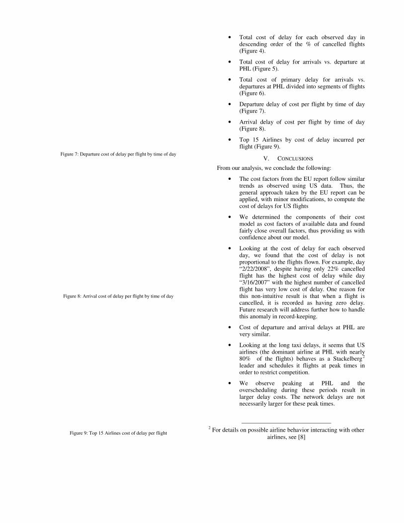
Figure 7: Departure cost of delay per flight by time of day

Figure 8: Arrival cost of delay per flight by time of day

Figure 9: Top 15 Airlines cost of delay per flight

: Departure cost of delay per flight by time of day

: Arrival cost of delay per flight by time of day

flight

• Total cost of delay for each observed daydescending order of the(Figure 4).

• Total cost of delay for arrivals vs. departure at PHL (Figure 5).

• Total cost of primary departures at PHL divided into seg(Figure 6).

• Departure delay of cost per flight by time of day(Figure 7).

• Arrival delay of cost per flight by time of day(Figure 8).

• Top 15 Airlines by cost of delay incurred per flight (Figure 9).

V. CONCLUSIONS

From our analysis, we conclude the following:

• The cost factors from the EU report trends as observed usinggeneral approach taken by the EU report can be applied, with minor modifications, cost of delays for US flights

• We determined the components of their costmodel as cost factors of available data and found fairly close overall factorsconfidence about our model.

• Looking at the cost of delay day, we found that the cost of delay is not proportional to the flights flown. For example, day “2/22/2008”, despite having only 22% cancelled flight has the highest cost of delay while day “3/16/2007” with the highest number of cancelled flight has very low cost of delay.this non-intuitive result is that when a flight is cancelled, it is recorded as having zero delay. Future research will address further how to handle this anomaly in record-keeping.

• Cost of departure and arrival very similar.

• Looking at the long taxi delays, it seems that US airlines (the dominant airline at PHL80% of the flights) behaves as a Stackelbergleader and schedules it flights at peak times in order to restrict competition

• We observe peaking at PHL and the overscheduling during these periods larger delay costs. The network delays are not necessarily larger for these peak times.

2 For details on possible airline behavior interacting with other

airlines, see [8]

Total cost of delay for each observed day in of the % of cancelled flights

Total cost of delay for arrivals vs. departure at

primary delay for arrivals vs. departures at PHL divided into segments of flights

ture delay of cost per flight by time of day

Arrival delay of cost per flight by time of day

Top 15 Airlines by cost of delay incurred per

ONCLUSIONS

conclude the following:

from the EU report follow similar observed using US data. Thus, the

general approach taken by the EU report can be applied, with minor modifications, to compute the cost of delays for US flights

ined the components of their cost as cost factors of available data and found

fairly close overall factors, thus providing us with confidence about our model.

Looking at the cost of delay for each observed we found that the cost of delay is not

proportional to the flights flown. For example, day “2/22/2008”, despite having only 22% cancelled flight has the highest cost of delay while day “3/16/2007” with the highest number of cancelled flight has very low cost of delay. One reason for

tuitive result is that when a flight is cancelled, it is recorded as having zero delay. Future research will address further how to handle

keeping.

departure and arrival delays at PHL are

axi delays, it seems that US dominant airline at PHL with nearly

) behaves as a Stackelberg2 ader and schedules it flights at peak times in

restrict competition.

We observe peaking at PHL and the g during these periods result in

The network delays are not necessarily larger for these peak times.

ble airline behavior interacting with other

airlines, see [8]

• One interesting result shows that not all airlines incur similar delay costs at PHL. Southwest, United Airlines, Delta Airlines and American Airlines all have higher costs of delay at PHL than does the dominant carrier, US Airways. Also, the regional airlines have lower costs of delay than the larger ones. Here too, the issue may be one of the way in which the data is recorded. The regional jets are more likely to be cancelled than the larger aircraft and, when cancelled, the data records such flights as having zero delay.

• Our calculations of the cost of delayed flights (but not cancelled flights) totals $18M for these 8 days.

Many modeling and analysis efforts require a good understanding of the costs that an airline will incur when it experiences delays at the gate, while taxiing or while en-route. This paper has presented a relatively straightforward mechanism for calculating such costs and for predicting how such costs are likely to increase when there is a change in fuel costs, aircraft type, or other major alternative in the cost structure. It is informative in explaining why airlines are currently down-gauging the size of the aircraft used even at airports with substantial capacity restrictions.

VI. FUTURE WORK

We intend to both expand and apply this model in a variety of efforts currently underway:

• Firstly, we need to include the costs of cancellations

into the model.

• We wish to apply the model and investigate its sensitivity to significant cost changes in fuel or crew, and changes in aircraft usage. Having a mechanism to understand costs by aircraft type allows us to use the model for aircraft not in the EU study.

• We intend to apply this model to a variety of different airports and see how airline costs vary based on different mixes of aircraft, varying amounts of airline dominance, and alternative government policies (such as slot-controls, rules about entry into the airport, etc.)

• We intend to examine if, based on these costs, we can predict which flights are most likely to be

cancelled or delayed when weather conditions result in the initiation of a ground-delay program.

• Once this model has been validated for a variety of different congestion scenarios and airports, we intend to include the model as part of a larger equilibrium model that predicts the actions of airlines under various policy decisions. See [9] for more on this effort.

• We intend to use this as a tool in a congestion-pricing model to determine the flights that are most likely to be cancelled first when capacity at an airport is reduced, and thereby to determine the prices that would be needed to have supply approximately equal demand if congestion pricing where imposed at some airport imposed.

REFERENCES

[1] C. E. Schumer, “Flight Delays Cost Passengers, Airlines and the U.S. Economy Billions”. A Report by the Joint Committee Majority Staff, May 2008.

[2] Performance Review Unit, Eurocontrol, “Evaluating the True Cost to Airlines of One Minute of Airborne or Ground Delay,” University of Westminster Final Report, May, 2004.

[3] (Online) Bureau of Transportation Statistics (BTS) Databases and Statistics. http://www.transtats.bts.gov/

[4] (Online) Air Transport Association of America, Inc (ATA), cost of delays. http://www.airlines.org/economics/cost+of+delays/ (2008).

[5] (Online) ICAO Engine Emissions databank, ICAO Committee on Aviation Environmental Protection (CAEP), hosted on UK Civil Aviation Authority, http://www.caa.co.uk/default.aspx?catid=702 (Updated Feb 2009).

[6] Beatty R, Hsu R, Berry L & Rome J,”Preliminary Evaluation of Flight

Delay Propagation through an Airline Schedule”,2nd USA/Europe Air Traffic Management R&D Seminar,December 1998

[7] (Online) Aviation System Performance Metrics (ASPM)-Complete. FAA, http://aspm.faa.gov/aspm/entryASPM.asp

[8] J. K. Brueckner, Internalization of airport congestion: A network analysis, International Journal of Industrial Organization, Elsevier, vol. 23(7-8), pages 599-614, September 2005

[9] L. Le “Demand Management at Congested Airports: How far are we from Utopia?”, PhD Dissertation, Systems Engineering and Operations Research Department, George Mason University, VA (July 2006)

APPENDIX

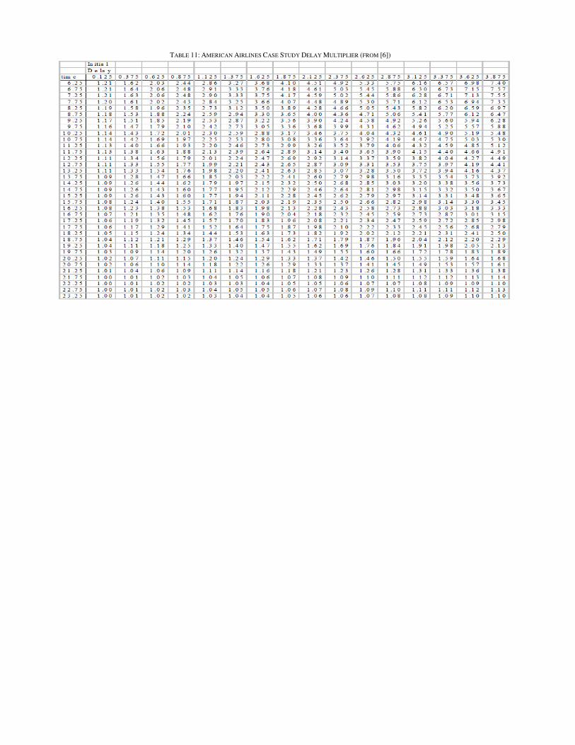
TABLE 11: AMERICAN AIRLINES CASE STUDY DELAY MULTIPLIER (FROM [6])