estimating deformations of random processes for correlation modelling: methodology and the...

Quarterly Journal of the Royal Meteorological Society Q. J. R. Meteorol. Soc. (2012)

Estimating deformations of random processes for correlationmodelling: methodology and the one-dimensional case

Y. Michel*CNRM-GAME/GMAP/RECYF, 42 av. G. Coriolis, 31057 Toulouse Cedex, France

*Correspondence to: CNRM-GAME/GMAP/RECYF, 42 av. G. Coriolis, 31057 Toulouse Cedex, France.E-mail: [email protected]

We introduce the use of spatial deformations for the modelling of background-error correlations in data assimilation with large dimensions of the state variable.Usually, the background-error covariance matrix is split into standard deviationsand correlations. In this framework, a proposal is made to model the correlations asthe space deformation of a stationary correlation model. The ‘shape from texture’approach introduced in the computer vision community is an algorithm thatestimates the relative deformation gradient and relies on a continuous waveletanalysis. It is also shown that it is possible to estimate the deformation gradientfrom a simple length-scale diagnosis and both approaches are compared. Then, achange of coordinate is derived from the numerical integration of the deformationgradient, opening the path to build the approximate correlation model.

Many variational data-assimilation schemes use a square-root form to constructthe background-error covariance matrix and it is shown how the deformationcan be easily included in such a formulation. This approach is of interest inallowing for objective geographical inhomogeneities of the structure functions. Thedeformed matrix is of slightly reduced rank, but this can be compensated for by aregularization. There is no need for additional normalization as is the case whenone models correlations with wavelet frames or recursive filters. The algorithm hasa similar computational cost to these two other approaches. Results are illustratedwith real data from one-dimensional temperature forecast errors produced by anoperational atmospheric model. Copyright c© 2012 Royal Meteorological Society

Key Words: wavelet; covariance; texture; data assimilation; background error

Received 15 March 2011; Revised 22 June 2012; Accepted 27 June 2012; Published online in Wiley Online Library

Citation: Michel Y. 2012. Estimating deformations of random processes for correlation modelling:methodology and the one-dimensional case. Q. J. R. Meteorol. Soc. DOI:10.1002/qj.2007

1. Introduction

Data assimilation makes extensive use of covariance modelsto describe the statistical structure of the errors thatare present in short-term forecasts, observations andalso sometimes the numerical model. In operational dataassimilation for the atmosphere and ocean, the size of thesecovariance matrices is currently of the order of 1012–1016

elements, which makes them difficult to estimate even on thebasis of the totality of observational information available(Dee, 1995). Therefore, a statistical model is required.Covariance estimation may for instance be obtained from

the diagonal coefficients in a basis defined a priori.This dramatically reduces the number of coefficients toestimate and therefore reduces sample noise, but can alsoapproximate the true covariance poorly if the basis is notwisely chosen. The covariance operator of a stationaryprocess has eigenvectors that are spectral functions (Mallatet al., 1998). In spherical geometry, isotropic background-error covariance (or correlation) functions have beendefined by means of positive Legendre expansions (Boer,1983; Courtier et al., 1998). On the plane, for limited-areamodels, space-stationary covariance models can be definedwith expansion in terms of bi-Fourier harmonics (Berre,

Copyright c© 2012 Royal Meteorological Society

Y. Michel

2000). In the ocean, because of the presence of coastlines,covariances are usually formulated directly in physical (grid-point) space. The fact that the integral solution of thediffusion equation defines a covariance operator was usedby Weaver and Courtier (2001) to construct covarianceoperators on the sphere. Another widespread method thathandles boundaries easily is the recursive filter approach,which is a convolution with a quasi-Gaussian self-adjointsmoothing kernel (Purser et al., 2003a). More general shapesand inhomogeneity can be represented (Purser et al., 2003b),but anisotropy comes at the price of significant mathematicaldevelopment (Purser et al., 2007). The relation betweenrecursive filters and the implicit diffusion equation in onedimension was explained by Mirouze and Weaver (2010).In the atmosphere, covariance matrices have also beencomputed from a diagonal assumption in a wavelet frameon the sphere (Fisher, 2004). A wavelet diagonal approachamounts to locally averaging the correlations (Pannekouckeet al., 2007). In a limited-area domain, Deckmyn and Berre(2005) studied a covariance matrix that is diagonal in anorthogonal basis made of non-dyadic Meyer wavelets.

Another method for building non-stationary covariancemodels is the change of coordinate, also called deformationor warping. Desroziers (1997) discussed a coordinatetransform based on semi-geostrophic theory (Hoskins,1975). The author postulated that correlations were isotropicin geostrophic (transformed) space, and showed that inphysical space the correlations in the vicinity of a frontwere contracted in the horizontal but also vertically tilted.The approach also has possible shortcomings: the transformhas to be relaxed in the Tropics, it only applies to largescales of motion and it does not depend on the observationnetwork. This kind of coordinate change has also beenconsidered along the vertical: Benjamin (1989) performedanalyses on isentropes (rather than isobaric surfaces) in theatmosphere and Weaver and Courtier (2001) illustrated theeffect on correlations of a transform from geopotential toisopycnal coordinates in the ocean. Thus, although thesetransforms allow the incorporation of ‘flow dependence’into the correlation structure, generally it has not beenproven extensively that the resulting flow dependence iscorrect. The transform does not depend on the observationnetwork, which has been shown to have a strong influenceon background errors (Bouttier, 1994; Belo-Pereira andBerre, 2006). This is believed to be a drawback, especiallyin atmospheric data assimilation, where observationaldata is overall abundant but has a very inhomogeneousdistribution, in particular because of the land–sea mask andthe distribution of clouds (McNally, 2002).

Recently, the Ensemble Kalman Filter (Evensen, 2003)and the ensemble of 4D-Var with perturbed observations(Fisher, 2003) have been shown to provide flow-dependentestimates of background-error statistics. As these ensemblesbecome more and more available on a routine basis, thereis strong interest in building operational schemes withtime- and space-varying background-error statistics. Onepossibility is to use a hybrid formulation (Hamill and Snyder,2000). Another is to use inhomogeneous and anisotropiccovariance models that are calibrated on the ensemble ofthe day (Berre and Desroziers, 2010). The structure ofthe background-error covariance matrix generally adoptedin operational centres is described in Bannister (2008b).It is generally built from a sequence of operators thatdescribe multivariate aspects on one hand and horizontal

and vertical covariances on the other hand. It is proposedhere to construct the autocovariance part of B as

V1/2(DSDT)VT/2, (1)

where V is a diagonal matrix of standard deviations, D isthe deformation operator and S a spatially stationary matrixobtained from the variance in spectral space. DSDT is rank-deficient, but can be turned into a ‘valid’ covariance matrixby the addition of a small regularization term. D is nevercomputed explicitly: only its effect on a control vector isneeded (as well as the adjoint). In practice, this effect is achange of coordinate and it is implemented using standardinterpolation techniques.

The original approach of using deformations has beenintroduced by Sampson and Guttorp (1992). More generally,classes of non-stationary processes that result from thedeformation of stationary processes have been studied indetail by Clerc and Mallat (2003). The estimation of thedeformation gradient in one and two dimensions, andits application to the ‘shape from texture’ problem hasbeen carried out by Clerc and Mallat (2002, hereafterCM02), using tools suitable for large grids. Leveraging thisprevious work, section 2 introduces continuous waveletanalysis and the texture gradient equation. Section 3 studiestwo estimators for the deformation numerically: the onedefined in CM02 based on wavelets and a second one basedon a local length-scale diagnosis. Section 4 illustrates thepotential of the method for the modelling of background-error covariances. This article focuses on the modelling of theautocorrelation part of B in atmospheric data assimilation. Itmay also prove useful in the ocean, and for other covariancematrices that need to be modelled.

2. The shape from texture approach

2.1. The problem in computer vision

‘Shape from texture’ is an inverse problem in computervision where the goal is to recover the shape of a surfacein a scene that is seen under perspective projection. Thissurface is covered by a texture, which may be understoodeither deterministically (the repetition of a texture element,or pattern) or stochastically (from the realization of arandom process). ‘Shape from texture’ has been extensivelystudied (Kanatani and Chou, 1989; Garding, 1992; Malik andRosenholtz, 1997). The problem is generally broken into twoindependent steps: firstly, analysis of the image, providingmeasurements of the texture distortion, and secondly thegeometrical problem of recovering the surface coordinates.CM02 chose to estimate the deformation gradient witha wavelet analysis in one dimension and a directionalwavelet analysis (or warplet) on the plane. The first partof the ‘shape from texture’ algorithm is of great interest forbackground-error correlation modelling in data assimilationand is described in this section.

2.2. Continuous wavelet analysis

Let R be a zero-mean stochastic process that is wide-sensestationary:

E{R(x)} = 0,

E{R(x)R(y)} = σ 2R cR(y − x),

Copyright c© 2012 Royal Meteorological Society Q. J. R. Meteorol. Soc. (2012)

Deformed Covariances

Figure 1. Wavelet analysis of a stationary process.

where E is the mathematical expectation, σR the constantstandard deviation and cR the homogeneous correlationfunction (Gaspari and Cohn, 1999). A deformation D actson a realization R as a warping or change of the coordinatex:

W(x) = DR(x) = R[d(x)], (2)

where d is a monotonic invertible function.Let ψ be a function the integral of which vanishes, called

the mother wavelet. The atomic wavelets are defined as

ψu,s(x) = 1

sψ

(x − u

s

), (3)

where ψu,s is a scale-dilated and translated version of themother wavelet. The process W is analyzed in both scaleand position using a continuous wavelet transform (Mallat,1999):

ω(u, s) = E{|〈W , ψu,s〉|2}, (4)

where ωu,s is called the scalogram; it is the expected varianceof the process in wavelet space using the usual innerproduct 〈〉 on L2(R). The scalogram is very similar tothe variance coefficients computed in the so-called waveletdiagonal assumption in covariance modelling (Fisher, 2004;Deckmyn and Berre, 2005; Pannekoucke et al., 2007) exceptthat here the wavelet transform is continuous and thereforeredundant.

When applied to a stationary process R, the scalogramdoes not depend on the position u:

d

duE{|〈R, ψu,s〉|2} = 0. (5)

This is illustrated in Figure 1, which depicts (a) onerealization of a stationary random process R and (b) itsscalogram computed from 10 000 independent realizations,

Figure 2. The correlation function of R (solid line) and the squaredcorrelation function of R′ (dashed line).

using the Sombrero wavelet (see section 3). The correlationfunction is chosen to belong to the Matern class (Rasmussenand Williams, 2006) with ‘smoothness’ parameter ν = 1,corresponding to

cR(x) =(

1 +√

3 x

�

)exp

(−

√3 x

�

),

where the length-scale is chosen to be � = 250 km. On thecircle, it is built numerically from its Fourier spectrum. Thecorrelation is shown in Figure 2. This choice gives a meansquare differentiable processes (Rasmussen and Williams,2006). This choice is probably more realistic as regardssmoothness assumptions than the widely chosen squaredexponential, as discussed by Stein (1999). The algorithmactually applies to a ‘large’ class of correlation functions, asspecified below.

W , as defined in (2), is not stationary and thereforeits scalogram is not space-invariant. Wavelets have beenchosen as analysis functions because they migrate underaffine transforms for small scales s:

〈W , ψu,s〉 ≈ 〈R, ψd(u),d′(u)s〉, (6)

where the prime denotes spatial differentiation. The innerproduct of W with ψu,s is almost equal to the inner productof R with a deformed wavelet at position d(u) and of scaled′(u)s. As a direct consequence, the scalogram also migrates:

E{|〈W , ψu,s〉|2} ≈ E{|〈R, ψd(u),d′(u)s〉|2}. (7)

Differentiating (4) and using (5) and (7) yields the ‘texturegradient equation’ for the scalogram of W (Clerc and Mallat,2003, Theorem 3.1):[

1 + O(s)]∂u ω(u, s) − d′′(u)

d′(u)∂log sω(u, s) = 0. (8)

This equation states that at vanishing scales (s → 0) thescalogram of the deformed process W is transported in


Y. Michel

(a) The deviation of the deformation d(x)–x2πα

(b) The derivative of the deformation d'(x)

Figure 3. Deformation based on the Schmidt transform.

wavelet space by a velocity that is the deformation gradientd′′/d′. The texture gradient equation is analogous to theoptical flow equation for the estimation of apparent motion(Heitz et al., 2010). The estimation problem is howeversimpler here, as the velocity tends towards the deformationgradient, which depends solely on position.

The analysis of Clerc and Mallat (2003) specifies thecondition that must be fulfilled by cR for establishing (8):

cR(0) − cR(x) = |x|γ C(x), h > 0, C(0) > 0, (9)

with γ > 0, C(0) > 0 and C continuously differentiable inthe neighbourhood of 0. The estimation is therefore likelyto work for a wide range of correlation functions, includingthe exponential (Ornstein–Uhlenbeck process).

2.3. Illustration with a Schmidt transform

To illustrate the preceding equations, we adopt theframework suggested by Pannekoucke et al. (2007), wherethe deformation is set up as a Schmidt transform ina way similar to the variable mesh global NWP modelARPEGE from Meteo-France (Courtier et al., 1998; Yessadand Benard, 1995). The direct deformation is defined on thecircle as

d(x) = 2πa

[1

2− 1

πtan−1

(c · tan(

π

2− x

2a))]

,

where x ∈ [0, 2πa] is the geographical position, a the radiusof the Earth and c the stretching factor, c = 2.4 in thecurrent version of ARPEGE. The deformation is shown inFigure 3(a) and is represented as the (normalized) deviationfrom the identity mapping d(x) − x. The deformation willmove a signal to the left (right) when the deviation of thedeformation is positive (negative).

One realization of W is drawn in Figure 4(a). Length-scales are stretched or elongated by a factor d′ (Figure 3b)

Figure 4. Wavelet analysis of a deformed process.

that reaches its maximum c = 2.4 at the centre of thedomain. Finally, the scalogram of W is shown in Figure 4(b).Following (7), it is directly related to the scalogram of R (Figure 1(b)).

3. Estimating the deformation

3.1. The sample scalogram

Because of sampling noise, the original algorithm of CM02relied on ergodicity (use of spatial averages) to build robustestimates of the deformation gradient. In contrast, thisarticle will investigate the behaviour of the algorithm forvarying ensemble sizes. In practice, we do not have access tothe true scalogram but only to a few realizations, typicallyE = O(1 − 100), because of computational limitations inNWP. For instance, Meteo-France is running operationallya global ensemble of six members with 4D-Var assimilationof perturbed observations. The scalogram of both R andW sampled over six realizations is shown in Figure 5. It isstrongly affected by sampling noise compared with Figure 4.Some of the correlations between the coefficients that appearfor both scale and space dimensions are due to the wavelettransform itself (Farge, 1992). The sample scalogram is heredefined as the unbiased sample variance in wavelet space,computed over E independent realizations:

ω = 1

E − 1

E∑e=1

|〈W (e), ψu,s〉 − 〈W , ψu,s〉|2,

where 〈W , ψu,s〉 = 1E

∑Ee=1〈W (e), ψu,s〉 is the sample mean

over the independent realizations W1, · · · , WE.

3.2. Estimating the deformation gradient and the deforma-tion

Following the texture gradient equation (8), the relativedeformation gradient can be estimated as the ratio of the



(a) The sample scalogram of R

(b) The sample scalogram of W

Figure 5. Wavelet scalogram sampled over six independent realizations.

spatial and scale derivatives of the sample scalogram:

d′′(u)

d′(u)= ∂u ω

∂log s ω. (10)

This estimator only requires the estimation of the scalogramat a single scale s. The partial derivatives of the samplescalogram are also conveniently computed using thederivative of the wavelet itself, following the implementationof CM02. The wavelet transform at a given scale iscomputed by convolution using a fast Fourier transform(FFT) algorithm (Smith, 2007). The equations are valid forany wavelet and in practice there is little sensitivity to thewavelet choice. Different wavelets have different selectivityin scale and space (Farge, 1992). As the algorithm only uses asingle scale, it is preferable to have a high selectivity in spacefor our application. Here, in particular, results are presentedwith the wavelet that is the Laplacian of a Gaussian with twovanishing moments (the ‘Sombrero’).

In the one-dimensional case, the estimated deformationcan be recovered from a direct integration of the deformationgradient:

d′(x) = exp(

A +∫ x

0

d′′(v)

d′(v)dv

), (11)

d(u) =∫ u

0d′(x) dx + B, (12)

where A and B are arbitrary integration constants. Asexplained by CM02, it is natural to obtain non-uniquenessof the deformation, as translation or a global change of scaledoes not affect the property of stationarity. Working on thecircle imposes periodicity on the deviation of deformation.In our case this can be written as d(2πa) = d(0) + 2πa or,equivalently, ∫ 2πa

0d′(x) dx = 2πa. (13)

(a) The deviation of the deformationd(x)–x2πα


Figure 6. Results obtained with the wavelet-based algorithm with sixindependent realizations: (a) the recovered deformation (dashed line)compared with the true deformation (solid lines) and (b) the true andrecovered deformation gradients. The grey shading indicates the 90%uncertainty estimated over different statistical realizations of the algorithm.

This fixes the constant A. The choice B = 0 is also made forconvenience.

The results are presented in Figure 6 for the specific casewhere the scalogram is estimated with E = 6 realizations. Atypical result of the estimation is shown by dashed lines.It gives a very good estimate for the deformation (a)and also for the deformation derivative (b). The estimateddeformation is more regular than the estimated deformationderivative because of the integration (12). The estimationof the deformation derivative is visibly affected by randomnoise, by a large amount at the centre of the domain wherethe deformation derivative is largest.

This noise can be quantified from a statistical pointof view. For this purpose, the estimation procedure hasbeen applied over a large number of independent statisticalrealizations (Ns = 105). The grey areas in Figure 6 indicateareas within which 90% of the results fall, constructed from5% and 95% quantiles of the distribution. This confirmsthat the uncertainty in the deformation derivative is largerwhere the deformation derivative is largest. Also, there is nosign of systematic error (e.g. bias of the estimator). Theseresults confirm that the deformation can be estimated froma small ensemble in a robust way.

3.3. An estimation based on local length-scale diagnosis

Before investigating in more details the effect of sampling(E) and number of grid cells (G) on the recovery ofthe deformation, another estimator is introduced forcomparison. The wavelet migration property (6) shows thatsmall scales of R are multiplied by d′ through the deformationprocess. Thus, there is a possibility of estimating d′ bycomputing the ‘length-scale’ of the deformed process W .Several economical estimates have been recently introduced


Y. Michel

to compute local correlation length-scales. In particular, themethod of Belo-Pereira and Berre (2006, hereafter BPB) hasbecome popular, as it only requires computation of variancesand gradients of fields. The correlation length-scale for abackground error ε is obtained by

Lεx =

√√√√√ Var ε

Var(dε

dx

)−

(d

dx

√Var ε

) ,

where ‘Var’ denotes the variance. This formula can be writtenmore compactly when the background error is normalizedby its standard deviation η = ε/

√Var ε (Appendix A):

Lεx = 1√

Var η′(x), (14)

where the prime denotes spatial differentiation. The localcorrelation length-scale is inversely proportional to thestandard deviation of the spatial derivative of the normalizederror field. The length-scale defined by Daley (1993) is onlyvalid for stationary correlations; thus the BPB formulashould be derived under an assumption of local stationarityin the sense of Mallat et al. (1998). Formula (14) can,however, be applied to any non-stationary correlationfunction if we can take derivatives. The covariance of Wis

Cov[W(x), W(y)

] = σ 2R cR

[d(y) − d(x)

]. (15)

To take derivatives, we must make the assumption that d istwice differentiable and that R is mean-square differentiable.This means that cR is twice differentiable (Rasmussenand Williams, 2006), the covariance of W is also twicedifferentiable and W itself is mean-square differentiable,and that

Cov[W ′(x), W ′(y)

] = −σ 2R d′(x) d′(y) c′′

R

[d(y) − d(x)

].

(16)

In the particular case where x = y,

Var W ′(x) = −σ 2R c′′

R(0) d′(x)2.

Introducing LR and LW , the BPB length-scales of R and Wyield

d′(x) = LR

√Var W ′(x)

σR= LR

LW.

Therefore, one obtains d′ as the inverse of the BPB length-scale up to a multiplicative constant.

First, one may notice that this expression is not validfor any correlation function cR. Indeed, the conditionfor deriving the equations is second-order differentiabilityof cR, which is more restrictive than (9). In particular,it is not valid for an exponentially decaying function(Ornstein–Uhlenbeck process), in contrast to the wavelet-based estimator. The derivative of the deformation isobtained up to a positive multiplicative constant LR, whichis equivalent to the constant exp A in the wavelet-basedframework. In the rest of the article, the estimator of d′ arenormalized to match the periodicity condition (13).

(a) The deviation of the deformation d(x)–x2πα


Figure 7. Results obtained with the length-scale based algorithm with sixindependent realizations. Same legend as in Figure 6.

It is convenient to define a grid index 0 ≤ k ≤ G − 1 thatcorresponds to the real position xk = 2πak/(G − 1), whereG is the number of grid cells. The random variable Xk is setas the sample variance of W ′ at grid index k:

Xk = 1

E − 1

E∑e=1

(W ′

k − W ′k

)2,

where we use the shorthand W ′k = W ′(xk) and where W ′

k isthe sample mean at point k. The length-scale based estimatecan be written as

d′k =

√Xk

1

G

G∑g=1

√Xg

. (17)

Results are presented in Figure 7 with E = 6 realizations.There is clearly more uncertainty than with the waveletalgorithm (Figure 6), yet the deformation can be recoveredfrom a few realizations. There is no apparent bias. Anotherinteresting aspect in Figure 7(b) is that the error looksspatially correlated, having larger length-scale where thedeformation gradient is smaller. In the next section, thestatistical properties (bias, standard deviation and spatialcorrelation) of the wavelet-based estimator (10)–(11) andthe length-scale based estimator (17) are compared fordifferent ensemble sizes, using the theory of statistics whenpossible.

3.4. Statistical behaviour of the estimators: a comparison

It is difficult to derive analytical results for the wavelet-basedestimator because it is necessary to introduce the wavelet-reproducing kernel that characterizes the correlation of thecontinuous wavelet transform (Farge, 1992). For the length-scale based estimate, the estimate in (17) is a function of the



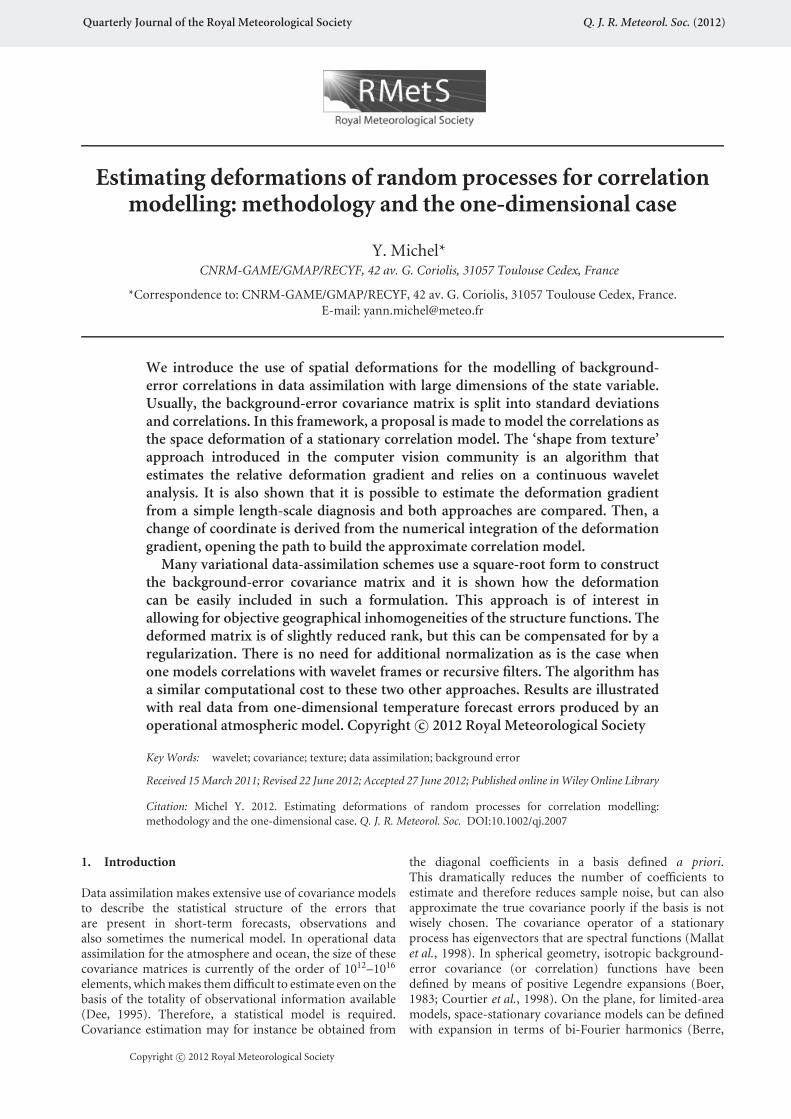
Figure 8. Convergence of the relative error in d′ at the centre of the domainas a function of ensemble size: the bias (stars) and standard deviation(circles) for the wavelet-based algorithm (solid lines) and length-scalebased algorithm (dashed lines).

variables Xk (or√

Xk). From the standard errors of Xk, itis possible to estimate the standard errors of this functionby Taylor expansions of functions of random variables asis classical in the theory of statistics (Kendall and Stuart,1977, chapter 10), and it is natural to start by describing thestatistical properties of Xk.

Xk is the unbiased estimator for the variance of W ′. Inthe case in which W ′ are independent observations from anormal distribution (which is the case here), the estimatorcan be verified:

E(Xk) = Var W ′k = −σ 2

R c′′R(0) d′

k2, (18)

Var(Xk) = 2

E − 1(Var W ′

k)2

= 2

E − 1σ 4

R c′′R(0)2 d′

k4. (19)

From a Taylor expansion (Appendix B), one can deducethat the standard error of the estimator of d′ will have thesame asymptotic decrease with ensemble size as the standarderror of Xk. The variance is of O(E−1) and thus the standarddeviation is of O(E−1/2). Bias and standard deviations of theestimators have been estimated from the 105 realizations,and they are drawn in Figure 8 as a function of ensemble sizeE. The bias is always negligible for both algorithms and thestandard deviation decays as O(E−1/2). The wavelet-basedalgorithm has lower standard error by roughly a factor of 3,consistent with what was found for the specific case E = 6illustrated in Figures 6(b) and 7(b).

A multidimensional version of (19) relates the covarianceof the sampling variance to the covariance of W ′ (Muirhead,2008):

Cov(Xk, Xl) = 2

E − 1

[Cov(W ′

k, W ′l )

]2. (20)

Using (16), it is possible to compute the spatial correlationof ‘noise’ Xk − EXk:

Corr(Xk, Xl) =[

c′′R(dl − dk)

c′′R(0)

]2

. (21)

The correlation function [c′′R/c′′

R(0)]2 is shown in Figure 2.It has a much shorter length-scale than cR, the correlationfunction of R. The noise has spatial correlation thatis non-stationary because of the deformation and thisis in agreement with Figure 7(b) (see also the Taylorexpansion in Appendix B for more details). For thewavelet-based estimator, the noise also appears to becorrelated in Figure 6(b). From the 105 realizations, it ispossible to compute the spatial correlation of the noisefor both algorithms. The result is shown in Figure 9 andclosely follows the analytical approximation (21). The noisecorrelation obtained with the wavelet-based estimator isslightly larger than that obtained with the length-scalebased estimator, and both correlation functions are non-stationary. This may be important in the case in which onewould like to design a noise-filtering algorithm to improvethe estimators.

3.5. Fewer grid cells

So far, we have assumed that the number of grid cells is largeenough that the texture gradient equation (8) is exact forthe wavelet-based estimator, and that the computation ofderivatives W ′ is exact for the length-scale based estimator.Both schemes will suffer from discretization errors when thisis not the case. Analytical study is possible by replacing W ′ bya finite-difference approximation, but this is cumbersome.Numerical experiments (not shown) indicates that thelength-scale based estimator is biased when the numberof grid cells is small, with underestimation (overestimation)of large (small) deformation gradients. This is especiallyapparent if W ′ is computed with finite differences, but itis less pronounced if derivatives are computed in spectralspace as is the case here. The wavelet-based estimator isless robust for small grid sizes, because the texture gradientequation has an error of O(s) where s is the scale in (3).Random fluctuations and this truncation error may causethe term ∂log sω to become small or even negative at somepositions. As this term is in the denominator in (10), this willcause failure of the algorithm. An illustration of this is givenin Figure 10. Spatial smoothing can improve the estimatorat the expense of introducing bias (CM02), but clearly bothalgorithms are more precise with a large number of gridcells.

4. Application to the modelling of background-errorcovariances

In general, any correlation function is not the deformationof a stationary one, as studied by Perrin and Senoussi(1999). In this section, the deformation approach is appliedto the modelling of correlations in atmospheric dataassimilation. Stationary correlation models are still widelyused (Bannister, 2008b), such that the approach can beappealing, especially as the deformation is easily put intothe variational framework on top of a stationary correlationmodel.


Y. Michel

(a) Wavelet-based estimator (b) Length-scale based estimator

Figure 9. Correlation of the noise Xk–EXk for (a) the wavelet-based estimator and (b) the length-scale based estimator for an ensemble size E = 6 (blacklines). Also shown is the analytical approximation obtained from theory and valid for the noise correlation of the sample variance of W ′ (grey lines) from(21).

Figure 10. A case of failure of the wavelet-based algorithm in the caseof small grid size (here G = 256 and E = 1): (a) estimation of ∂log sω thatbecomes small at the location indicated by the bold arrow and (b) erroneousestimation of d′.

4.1. Variational data assimilation

In the incremental formulation (Courtier et al., 1994), avariational 3D- or 4D-Var scheme is framed to providean analysis xa that minimizes a cost function J(x) given abackground forecast xb:

δx = x − xb,

J(δx) = Jb(δx) + Jo(δx)

= 1

2δxTB−1δx + 1

2(Hδx − δy)TO−1(Hδx − δy),

where the time index has been dropped for convenience,and where

• B is the background-error covariance matrix;• O is the observation-error covariance matrix;• δy = y − H(xb) is the innovation vector, the depar-

ture between the observation and the backgroundin observation space, with H being the nonlinearobservation operator.

The minimization problem can be derived from a Bayesianpoint of view, as detailed by Lorenc (1986). The modelledbackground-error covariance matrix B approximates thetrue background-error covariance matrix, which is a crudeassumption in some cases (in particular, B is often takenas static). In incremental 4D-Var, H also includes theintegration in time of a linear model describing the evolutionof small perturbations.

The use of the variable δx = B1/2u, where B1/2 is a squareroot of B, reduces the cost function to

J(u) = 1

2uTu + 1

2(HB1/2u − δy)TO−1(HB1/2u − δy).

This change of variable generally improves the conditioningof the minimization, which results in faster convergence(Lorenc, 1997; Gauthier et al., 1999). B1/2 is convenientlymodelled as a sequence of operators, as reviewed in Bannister(2008b). A generic form for B1/2 is

B1/2 = KpV1/2S1/2,

where Kp is the balance operator that describes multivariateaspects (Derber and Bouttier, 1999). V1/2 accounts forgeographically varying variances and S1/2 models stationarycorrelations, for instance with recursive filters or in spectralspace. Adding deformation in this sequence gives themodelling

B1/2 = KpV1/2DS1/2, (22)



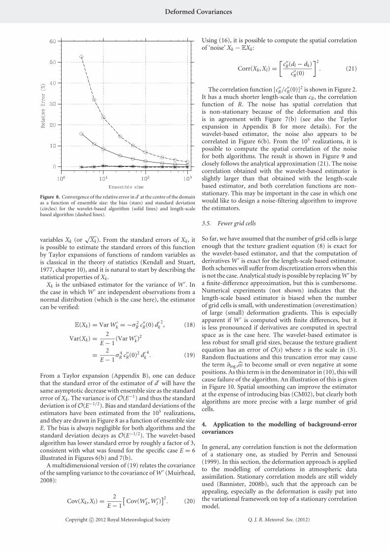
where the (linear) operator D is the discrete implementationof the change of variable (2). For instance, the nearest-neighbour interpolation scheme of a vector r at grid index kis

(Dr)k = rdk+0.5�, (23)

where dk is the deformation (new coordinate) at grid pointk. The linear interpolation is

(Dr)k = rdk� + (r�dk − rdk�)(dk − dk�). (24)

The standard Hermite cubic spline is also used (third-degreesplines with each polynomial of the spline in Hermite form).Two important remarks can be made: the modelled matrixDSDT is of reduced rank, but it can be regularized into avalid covariance matrix DSDT + λS with 0 < λ � 1. S isnow the correlation matrix of the undeformed variables andis computed from the power spectrum of the undeformederror samples.

4.2. Application to ARPEGE forecast errors

In this section, operational ARPEGE forecasts are usedto construct samples of background errors, using the‘NMC’∗ method (Parrish and Derber, 1992). This methodhas the drawback of overestimating correlation length-scales (Belo-Pereira and Berre, 2006) and the statisticsoften require adjustments to counteract these effects, butit is generally suitable for estimation of climatologicalcovariances (Bouttier, 1996; Bannister, 2008a) and thereforesufficient for our purpose. One realization of such a sample isshown in Figure 11(a). Samples are differences between 48 hand 24 h forecasts valid at the same time, for the temperaturevariable at 1000 m height, extracted on a parallel (at 40◦N)and normalized by the sample standard deviation. Thischoice is motivated by the fact that correlations for these dataappear to be inhomogeneous. The number of grid pointsis 720. The ensemble is composed of 100 fields averagedduring the months of November and December 2011. Theassociated scalogram analysis is shown in Figure 11(b). Theerror statistics are not space-invariant, with, in particular,more energy being noticeable at smaller scales over Europe(0–40◦E).

The sample correlation functions are shown in Figure 12and appear noisy because of sampling error (there are 100members of 720 grid points compared with 7202 valuesto estimate). As in the ensemble Kalman filter (Evensen,2003), an efficient filtering of larger scales of the correlationfunction is performed with a Schur product (Hamill et al.,2001) with the standard compactly supported correlationfunction of Gaspari and Cohn (1999). This methodology isalso frequently referred to as localization or matrix tapering.It appears reasonable to model these correlations as thedeformation of a single correlation function, as correlationshave roughly the same global shape but different length-scales, in particular shorter ones over Europe and largerones over the Himalaya mountains (100◦E), consistent withthe scalogram in Figure 11.

Direct application of the estimators defined in theprevious section give very similar results, as shown in

∗The National Meteorological Center, now the National Centers forEnvironmental Prediction (NCEP).

(a) A realization of normalized ARPEGE forecast error

(b) The wavelet scalogram (average over 100 realizations)

Figure 11. Wavelet analysis of ARPEGE forecast errors in temperature.

Figure 12. Sample correlations for ARPEGE temperature backgrounderrors filtered with a compactly supported Schur product as a function oflongitude.

Figure 13. The wavelet-based and length-scale basedestimated deformations are in very good agreement.Locations where the deviation of deformation is a decreasingfunction (between 180◦W and 60◦W and again between 60◦Eand 180◦E) are the locations of large scales in the scalogram(Figure 11) and of wider sample correlations (Figure 12),and the same is true for small scales.


Y. Michel

Figure 13. Estimated deviations of deformation with the wavelet-basedalgorithm (solid line) and the length-scale based algorithm (dashed line).

Figure 14. Variances for three different interpolations D: variance-conserving piecewise interpolation (blue lines), linear interpolation (redlines) and linearized spline interpolation (green lines).

4.3. Modelled correlations

One advantage of the deformed approach is that there is noneed to correct for a variance term as is the case with thewavelet diagonal assumption (Fisher, 2004; Pannekouckeet al., 2007), the recursive filter (Purser et al., 2003b; Micheland Auligne, 2010) or the diffusion equation (Weaver andCourtier, 2001; Mirouze and Weaver, 2010). This is becausethe deformation will preserve the variance:

E{W(x)2} = E{R(d(x)

)2} = σ 2R .

In the discrete case, this is only true up to interpolationerrors. The diagonal of the matrix DSDT is representedin Figure 14 for three classical interpolation schemes. Thevariances are exactly conserved by the nearest-neighbourinterpolation. They are still of sufficient accuracy in thelinear and spline interpolations, so that DSDT does not needto be normalized.

The modelled correlations are shown in Figure 15 withspline interpolation. The stationary correlations modelledwith a diagonal spectral approach are also drawn forreference. The deformed correlations incorporate spatialvariations also seen in the sample correlation functions(Figure 12), in particular at smaller length-scales overEurope and larger ones over the Himalayas. The longerrange correlations are less noisy than with the Schur-filteredsample correlations, as they are a smooth deformation ofthe globally averaged correlation function.

Without regularization, the space dimension of theanalysis increment will be reduced by some amount. Itis non-trivial to estimate the rank of DSDT. Indeed, thematrix form of D is never computed and the deformationis only available as a ‘black-box’ operator defined by itsaction on a vector (2). Estimating the rank (or the smallesteigenvalues) of such a large matrix using randomizationis the topic of active research (Sorensen, 2002). In the

Figure 15. Modelled correlations as a function of longitude using splineinterpolations (solid lines), compared with the stationary spectral model(dashed lines).

one-dimensional context considered here, it is possibleto compute explicitly the matrices DSDT of dimensions720 × 720 and their rank. For the nearest-neighbour, linearand spline interpolations, we obtain values of respectively618, 620 and 620. This confirms that in practice, at least forslowly varying deformations, only a small rank reductionoccurs. If not, then regularization is easily implemented atthe expense of requiring more memory.

4.4. Computational aspects

In this section, the numerical cost of applying theautocovariance part of B1/2 is compared for differentformulations. The deformation is based on interpolation,for which efficient implementations of the need to integratethe model in time generally exist. Applying the operator Dis equivalent to performing an interpolation and thereforethe associated cost scales as G, where G is the numberof grid cells. Applying the stationary part through theoperators S1/2 has the cost of an FFT, and therefore scales asG log G. In comparison, the transform based on the diagonalassumption in a wavelet frame can be applied in G or G log Goperations, depending on whether filter banks or FFTs areused (Mallat, 1999). The recursive filters can be applied inoG operations, where o ≈ 4 is the order of the recursive filteras described in Purser et al. (2003a).

It is of interest to include the cost of the calibrationpart in the comparison, as some NWP centres withvariational assimilation move towards a recomputation ofthe background-error model on a seasonal or even a dailybasis, in order to incorporate flow dependence. For thedeformation, the calibration part is also computationallyfeasible, as one only needs to compute the wavelet transformat a single scale. Thus the overall cost of the calibrationpart scales as EG log G, where E is the number of ensemblemembers. The calibration part of the wavelet scaling requirescomputation of variances in wavelet space, and scales as EG



or EG log G. The calibration of the recursive filter requiresa length-scale diagnosis. Following Belo-Pereira and Berre(2006), this requires computation of variances and canbe implemented efficiently in EG operations (or EG log G ifderivatives are taken in spectral space). Then, the coefficientsof the recursive filters need to be computed from a Choleskidecomposition. This has been implemented, relying heavilyon the band structure of the matrices of interest, in o2G/3operations in Michel and Auligne (2010). Thus, both thecalibration part and the application of the operators canbe achieved at a similar cost, although computation of thenormalization for approaches other than the deformationone may change this.

5. Conclusion

We introduce for the purpose of geophysical dataassimilation an approximate correlation model that isbased on the objective deformation of a stationary one.The approach follows ideas from Sampson and Guttorp(1992). The algorithm of CM02 consists of estimatingthe deformation gradient from a continuous waveletanalysis. The scalogram of a deformed process obeys atransport equation, called the texture gradient equation. Thedeformation relative gradient plays the role of advection inwavelet space. These properties are illustrated first with atoy model, where correlations are stretched by a Schmidttransform on the circle, following a framework suggested byPannekoucke et al. (2007).

This article introduces a novel estimator for thedeformation based on the computation of local correlationlength-scales as introduced by Belo-Pereira and Berre(2006). The deformation is the ratio between the length-scales of the original process and the deformed process.This property can be used to define a length-scale basedestimator and we compare its statistical properties with thoseof the wavelet-based estimator. Both algorithms have similardecay of the standard error as the ensemble size grows. Thewavelet-based estimator has lower standard deviation thanthe length-scale based estimator by roughly a factor of 3. Thenoise of the deformation derivative has a standard deviationapproximately proportional to the deformation derivative,and has non-stationary spatial correlation structure. Thelength-scale based estimator is biased when the number ofgrid cells is too small, because of truncation error in thecomputation of the derivative. The wavelet-based estimatoris likely to exhibit failures when the number of grid cells istoo small.

Once the deformation gradient is estimated, numericalintegration recovers the deformation itself. Together with apower-spectrum estimation, this constitutes an approximatecorrelation model for data assimilation. This matrix can beregularized into a valid covariance matrix if necessary. Thisnon-stationary correlation model can be used in variationaldata assimilation for the specification of background-errorstatistics. The approach is computationally reasonable even ifthe deformation has to be estimated online when computingthe covariance errors of the day. It does not requireadditional normalization. For certain applications, thiscan be a significant advantage over other inhomogeneousmodels, including the diagonal assumption in a waveletframe, inhomogeneous recursive filters or the generalizeddiffusion equation.

Application using real ARPEGE data shows that thewavelet-based and length-scale based estimators retrievesimilar deformations. This approximate correlation modelseems able to extract valuable information from theensemble, resulting in non-stationary correlation functionsfor data assimilation.

Further work will probably address the case of sphericalgeometry.

Acknowledgement

This research has been supported by the ANR projectGeoFluids under the reference ANR-09-SYSC-005.

A. Compact formulation of the BPB length-scale

The normalized background error is obtained by η =ε/σ (ε), where σ (ε) is the standard deviation σ (ε) =√

Var ε. Then

dη

dx=

dεdx σ (ε) − ε dσ (ε)

dx

σ (ε)2.

Because E{ε} = 0, E{ dη

dx } = 0 and the variance is

Vardη

dx

=Var ε Var dε

dx + Var ε[

dσ (ε)dx

]2 − 2 dσ (ε)dx σ (ε)E{ε dε

dx }(Var ε)2

.

Using the fact that

E{ε dε

dx} = E{1

2

dε2

dx} = 1

2

dσ (ε)2

dx= σ (ε)

dσ (ε)

dx,

the expression can be simplified to

Vardη

dx=

Var dεdx −

[dσ (ε)

dx

]2

Var ε,

which proves (14).

B. Use of Taylor expansions for the moments of functionsof random variables

The length-scale based estimator (17) can be expressed as afunction of the variables X1, · · · , XG. Following Kendall andStuart (1977, chapter 16), Xk follows a scaled χ2 distributionthat approaches normality as E → ∞, but at a ratherslow tendency. Fisher’s results shows that a square-roottransformation actually improves this convergence, so it isbetter to consider the length-scale based estimator as being afunction of the sample standard deviations

√X1, · · · ,

√XG.

These random variables are slightly biased, but in the casewhere W ′ is normally distributed a minor correction exists toeliminate the bias. Defining the variables Yg = c4(E)−1

√Xg ,

the length-scale based estimator (17) can be expressed as

d′k = G

Yk∑Gg=1 Yi

= Fk(Y1, · · · , YG) (B1)


Y. Michel

and the correction factor c4 depends on the sample size E asfollows:

c4(E) =√

2

E − 1

�(E/2)

�( E−12 )

= 1 − 1

4E+ O(E−2),

where �(·) is the classical extension of the factorialfunction, the gamma function. The random variables Yk

are approximately Gaussian, with mean and variance givenby

E(Yk) =√

Var W ′k = σR

√−c′′

R(0) d′k, (B2)

Var Yk = [c4(E)−2 − 1

]Var W ′

k

= − c′′R(0) σ 2

R

2Ed′

k2 + O(E−2). (B3)

As in Kendall and Stuart (1977, chapter 10), it is possible toapply a multidimensional Taylor expansion to the functionFk to obtain the variance of d′

k as a function of the mean,variance and covariances of Yk:

VarFk(Y) =G∑

i=1

{∂iFk

[E(Y)

]}2Var Yi

+G,G∑i �=j

∂iFk[E(Y)

]∂jFk

[E(Y)

]Cov(Yi, Yj) + o(E−1).

The mean and variance of Yk are given in (B2)–(B3), but itis also necessary to derive the covariance at leading order inE. Similarly, for two functions g(X) and h(X) we have theTaylor expansion (Kendall and Stuart, 1977, chapter 10)

Cov[g(X), h(X)

] =G∑

i=1

∂ig[E(X)

]∂ih

[E(X)

]Var(Xi)

+G,G∑i �=j

∂ig[E(X)

]∂jh

[E(X)

]Cov(Xi, Xj) + o(E−1).

Applying this formula with particular functions g(X) = √Xi

and h(X) = √Xj allows us to derive Cov(Yi, Yj) as a function

of Cov(Xi, Xj):

Cov(Yi, Yj) = ∂ig[E(X)

]∂jh

[E(X)

]Cov(Xi, Xj) + o(E−1)

= 1

2Ed′

i d′j

σ 2R

−c′′R(0)

[c′′

R(dj − di)]2 + o(E−1).

Using the variance of Yi given in (B3), one further finds thatthe correlations are the same at leading order:

Corr(Yi, Yj) = Corr(Xi, Xj) + o(1),

where this latter correlation has already been computed in(21). Then, evaluation of the partial derivatives of Fk yields

∂iFk = −GYk(∑G

j=1 Yj)2 if i �= k,

∂kFk = G

∑Gi=1,i �=k Yi( ∑G

j=1 Yj)2 .

Gathering all results yields the variance of the estimator atleading order in E:

VarFk(Y) = d′k

2

2EG−2

{ G∑i �=k

d′i2 + (G − d′

k)2

+G,G∑i �=j

i,j �=k

d′i d′

j

[c′′

R(dj − di)

c′′R(0)

]2

− (G − d′k)

G∑i �=k

d′i

c′′R(di − dk)2 + c′′

R(dk − di)2

c′′R(0)2

}+o(E−1).

This expression, in particular, makes explicit the fact thatthe variance depends on the correlation function cR and onthe number of grid cells G. It explains the O(E−1/2) decay ofthe standard error seen in Figure 8. For most applications,however, when the grid size is large and the correlationfunction narrow enough we can neglect the effect of gridsize and cR. The term in brackets is then almost equal toG2. The variance can be approximated with a much simplerexpression:

VarFk(Y) ≈ d′k

2

2E. (B4)

This approximation shows more clearly the fact that thenoise standard deviation is proportional to d′ as illustratedin Figure 7(b).

References

Bannister RN. 2008a. A review of forecast error covariance statisticsin atmospheric variational data assimilation. I: Characteristics andmeasurements of forecast error covariances. Q. J. R. Meteorol. Soc.134: 1951–1970.

Bannister RN. 2008b. A review of forecast error covariance statistics inatmospheric variational data assimilation. II: Modelling the forecasterror covariance statistics. Q. J. R. Meteorol. Soc. 134: 1971–1996.

Belo-Pereira M, Berre L. 2006. The use of an ensemble approach to studythe background error covariances in a global NWP. Mon. WeatherRev. 134: 2466–2489.

Benjamin SG. 1989. An isentropic mesoα-scale analysis system and itssensitivity to aircraft and surface observations. Mon. Weather Rev.117: 1586–1603.

Berre L. 2000. Estimation of synoptic and mesoscale forecast errorcovariances in a limited-area model. Mon. Weather Rev. 138: 644–667.

Berre L, Desroziers G. 2010. Filtering of background error variances andcorrelations by local spatial averaging: A review. Mon. Weather Rev.138: 3693–3720.

Boer G. 1983. Homogeneous and isotropic turbulence on the sphere. J.Atmos. Sci. 40: 154–163.

Bouttier F. 1994. A dynamical estimation of forecast error covariancesin an assimilation system. Mon. Weather Rev. 122: 2376–2390.

Bouttier F. 1996. ‘Application of Kalman filtering to numerical weatherprediction’. In ECMWF Seminar on Data Assimilation. ECMWF:Reading, UK; pp 61–90.

Clerc M, Mallat S. 2002. The texture gradient equation for recoveringshape from texture. IEEE Trans. Pattern Anal. Machine Intelligence24: 536–549.

Clerc M, Mallat S. 2003. Estimating deformations of stationary processes.Ann. Statist. 31: 1772–1821.

Courtier P, Andersson E, Heckley W, Vasiljevic D, Hamrud M,Hollingsworth A, Rabier F, Fisher M, Pailleux J. 1998. The ECMWFimplementation of three-dimensional variational assimilation (3D-Var). I: Formulation. Q. J. R. Meteorol. Soc. 124: 1783–1807.

Courtier P, Thepaut JN, Hollingsworth A. 1994. A strategy for operationalimplementation of 4D-Var, using an incremental approach. Q. J. R.Meteorol. Soc. 120: 1367–1387.



Daley R. 1993. Atmospheric data analysis. Cambridge University Press:Cambridge, UK.

Deckmyn A, Berre L. 2005. A wavelet approach to representingbackground error covariances in a limited-area model. Mon. WeatherRev. 133: 1279–1294.

Dee DP. 1995. On-line estimation of error covariance parameters foratmospheric data assimilation. Mon. Weather Rev. 123: 1128–1145.

Derber J, Bouttier F. 1999. A reformulation of the background-errorcovariance in the ECMWF global data assimilation system. Tellus51A: 195–221.

Desroziers G. 1997. A coordinate change for data assimilation in sphericalgeometry of frontal structures. Mon. Weather Rev. 125: 3030–3038.

Evensen G. 2003. The Ensemble Kalman Filter: Theoretical formulationand practical implementation. Ocean Dynamics 53: 343–367.

Farge M. 1992. Wavelet transforms and their applications to turbulence.Ann. Rev. Fluid Mech. 24: 395–458.

Fisher M. 2003. ‘Background error covariance modelling’. In ECMWFSeminar on recent developments in data assimilation for atmosphereand ocean. ECMWF: Reading, UK; pp 45–63.

Fisher M. 2004. ‘Generalized frames on the sphere, with application to thebackground-error covariance modelling’. In Proceedings of ECMWFSeminar on developments in numerical methods for atmospheric andocean modelling. ECMWF: Reading, UK; pp 87–101.

Garding J. 1992. Shape from texture for smooth curved surfacesin perspective projection. J. Mathematical Imaging and Vision 2:630–638.

Gaspari G, Cohn S. 1999. Construction of correlation functions in twoand three dimensions. Q. J. R. Meteorol. Soc. 125: 723–757.

Gauthier P, Charette C, Fillion L, Koclas P, Laroche S. 1999.Implementation of a 3D variational data assimilation system atthe Canadian Meteorological Centre. Part I: The global analysis.Atmos.–Ocean 37: 103–156.

Hamill T, Whitaker J, Snyder C. 2001. Distance-dependent filtering ofbackground error covariance estimates in an Ensemble Kalman Filter.Mon. Weather Rev. 129: 2776–2790.

Hamill TM, Snyder C. 2000. A hybrid ensemble Kalman Filter–3Dvariational analysis scheme. Mon. Weather Rev. 128: 2905–2919.

Heitz D, Memin E, Schnorr C. 2010. Variational fluid flow measurementsfrom image sequences: synopsis and perspectives. Exp. Fluids 48:369–393.

Hoskins B. 1975. The geostrophic momentum approximation and thesemi-geostrophic equations. J. Atmos. Sci. 32: 233–242.

Kanatani K, Chou TC. 1989. Shape from texture: General principle.Artificial Intelligence 38: 1–48.

Kendall SM, Stuart A. 1977. The Advanced Theory of Statistics, Vol. 1:Distribution Theory. C. Griffin and Co.: London and High Wycombe.

Lorenc AC. 1986. Analysis methods for numerical weather prediction.Q. J. R. Meteorol. Soc. 112: 1177–1194.

Lorenc AC. 1997. Development of an operational variational assimilationscheme. J. Meteorol. Soc. Jpn 75: 339–346.

Malik J, Rosenholtz R. 1997. Computing local surface orientation andshape from texture for curved surfaces. Int. J. Comput. Vision 23:149–168.

Mallat S. 1999. A wavelet tour of signal processing, 2nd edn. AcademicPress: New York.

Mallat S, Papanicolaou G, Zhang Z. 1998. Adaptive covariance estimationof locally stationary processes. Ann. Statistics 26: 1–47.

McNally AP. 2002. A note on the occurrence of cloud in meteorologicallysensitive areas and the implications for advanced infrared sounders.Q. J. R. Meteorol. Soc. 128: 2551–2556.

Michel Y, Auligne T. 2010. Inhomogeneous background error modelingand estimation over Antarctica. Mon. Weather Rev. 138: 2229–2252.

Mirouze I, Weaver A. 2010. Representation of correlation functions invariational assimilation using an implicit diffusion operator. Q. J. R.Meteorol. Soc. 136: 1421–1443.

Muirhead RJ. 2008. Samples from a Multivariate Normal Distribution,and the Wishart and Multivariate Beta Distributions. In Aspects ofMultivariate Statistical Theory. John Wiley & Sons, Inc: Hoboken, NJ;79–120.

Pannekoucke O, Berre L, Desroziers G. 2007. Filtering properties ofwavelets for local background-error correlations. Q. J. R. Meteorol.Soc. 133: 363–379.

Parrish D, Derber J. 1992. The National Meteorological Center’s SpectralStatistical-Interpolation analysis system. Mon. Weather Rev. 120:1747–1763.

Perrin O, Senoussi R. 1999. Reducing non-stationary stochastic processesto stationarity by a time deformation. Statist. Probab. Lett. 43:393–397.

Purser R, Pondeca SD, Parrish D, Devenyi D. 2007. ‘Covariancemodelling in a grid-point analysis’. In Proceedings of the ECMWFWorkshop on flow-dependent aspects of data assimilation. ECMWF:Reading, UK; pp 11–25.

Purser R, Wu W, Parrish D, Roberts N. 2003a. Numerical aspects of theapplication of recursive filters to variational statistical analysis. PartI: Spatially homogeneous and isotropic Gaussian covariances. Mon.Weather Rev. 131: 1524–1535.

Purser R, Wu W, Parrish D, Roberts N. 2003b. Numerical aspects of theapplication of recursive filters to variational statistical analysis. Part II:Spatially inhomogeneous and anisotropic general covariances. Mon.Weather Rev. 131: 1536–1548.

Rasmussen CE, Williams C. 2006. Gaussian processes for machine learning.MIT Press: Cambridge, MA.

Sampson PD, Guttorp P. 1992. Nonparametric estimation ofnonstationary spatial covariance structure. J. Amer. Statist. Assoc.87: 108–119.

Smith J. 2007. Mathematics of the Discrete Fourier Transform (DFT) withAudio Applications, 2nd edn. W3K Publishing: Stanford, CA.

Sorensen DC. 2002. Numerical methods for large eigenvalue problems.Acta Numerica 11: 519–584.

Stein M. 1999. Statistical interpolation of spatial data: Some theory forkriging. Springer: New York, NY.

Weaver A, Courtier P. 2001. Correlation modelling on the sphere using ageneralized diffusion equation. Q. J. R. Meteorol. Soc. 127: 1815–1846.

Yessad K, Benard P. 1995. Introduction of a local mapping factor inthe spectral part of the Meteo-France global variable mesh numericalforecast model. Q. J. R. Meteorol. Soc. 122: 1701–1719.


estimating deformations of random processes for correlation modelling: methodology and the...

Documents