Estimating Average Treatment Effects with Support Vector

Machines∗

Alexander Tarr† Kosuke Imai‡

July 2, 2021

Abstract

Support vector machine (SVM) is one of the most popular classification algorithms in the

machine learning literature. We demonstrate that SVM can be used to balance covariates

and estimate average causal effects under the unconfoundedness assumption. Specifically, we

adapt the SVM classifier as a kernel-based weighting procedure that minimizes the maximum

mean discrepancy between the treatment and control groups while simultaneously maximiz-

ing effective sample size. We also show that SVM is a continuous relaxation of the quadratic

integer program for computing the largest balanced subset, establishing its direct relation

to the cardinality matching method. Another important feature of SVM is that the regular-

ization parameter controls the trade-off between covariate balance and effective sample size.

As a result, the existing SVM path algorithm can be used to compute the balance-sample

size frontier. We characterize the bias of causal effect estimation arising from this trade-off,

connecting the proposed SVM procedure to the existing kernel balancing methods. Finally,

we conduct simulation and empirical studies to evaluate the performance of the proposed

methodology and find that SVM is competitive with the state-of-the-art covariate balancing

methods.

Keywords: causal inference, covariate balance, matching, subset selection, weighting

∗We thank Brian Lee for making his simulation code available and Francesca Dominici, Chad Hazlett, GaryKing, Jose Zubizarreta and seminar participants at Institute for Quantitative Social Science, Harvard Universityfor helpful discussions. An anonymous reviewer of the Alexander and Diviya Magaro Peer Pre-Review Programfor insightful comments. Imai thanks the Sloan Foundation (# 2020–13946) for financial support.

†PhD. Candidate, Department of Electrical Engineering, Princeton University, Princeton, NJ 08544.Email:atarr@princeton.edu

‡Professor, Department of Government and Department of Statistics, Harvard University, Cambridge, MA02138. Phone: 617–384–6778, Email: Imai@Harvard.Edu, URL: https://imai.fas.harvard.edu

arX

iv:2

102.

1192

6v2

[st

at.M

E]

1 J

ul 2

021

1 Introduction

Estimating causal effects in an observational study is complicated by the lack of randomization in

treatment assignment, which may lead to confounding bias. The standard approach is to weight

observations such that the empirical distribution of observed covariates is similar between the

treatment and control groups (see e.g., Lunceford and Davidian, 2004; Rubin, 2006; Ho et al.,

2007; Stuart, 2010). Researchers then estimate the causal effects using the weighted sample

while assuming the absence of unobserved confounders. Recently, a large number of weighting

methods have been proposed to directly optimize covariate balance for causal effect estimation

(e.g., Hainmueller, 2012; Imai and Ratkovic, 2014; Zubizarreta, 2015; Chan et al., 2016; Athey

et al., 2018; Li et al., 2018; Wong and Chan, 2018; Zhao, 2019; Hazlett, 2020; Kallus, 2020; Ning

et al., 2020; Tan, 2020).

This paper provides a new insight to this fast growing literature on covariate balancing by

demonstrating that support vector machine (SVM), which is one of the most popular classifica-

tion algorithms in machine learning (Cortes and Vapnik, 1995; Scholkopf et al., 2002), can be

used to balance covariates and estimate the average treatment effect under the standard uncon-

foundedness assumption. We adapt the dual coefficients for the soft-margin SVM classifier as

kernel balancing weights that minimizes the maximum mean discrepancy (Gretton et al., 2007a)

between the treatment and control groups while simultaneously maximizing effective sample size.

The resulting weights are bounded, leading to stable causal effect estimation. As SVM has been

extensively studied and widely used, we can exploit its well-known theoretical properties and

highly optimized implementations.

All matching and weighting methods face the same trade-off between effective sample size and

covariate balance with a better balance typically leading to a smaller sample size. We show that

SVM directly addresses this fundamental trade-off. Specifically, the dual optimization problem

1

for SVM computes a set of balancing weights as the dual coefficients while yielding the support

vectors that comprise a largest balanced subset. In addition, the regularization parameter of SVM

controls the trade-off between sample size and covariate balance. We use existing path algorithms

(Hastie et al., 2004; Sentelle et al., 2016) to efficiently characterize the balance-sample size frontier

(King et al., 2017). We analyze how this trade-off between sample size and covariate balance affect

causal effect estimation.

We are not the first to realize the connection between SVM and covariate balancing. Ratkovic

(2014) points out that the hinge-loss function of the primal optimization problem for SVM has

a first-order condition, which leads to balanced covariate sums amongst the support vectors.

Instead, we show that the dual form of the SVM optimization problem leads to the covariate

mean balance. In addition, Ghosh (2018) notes the relationship between the SVM margin and the

region of covariate overlap. The author argues that the support vectors correspond to observations

lying in the intersection of the convex hulls for the treated and control samples (King and Zeng,

2006). In contrast, we show that the SVM dual coefficients can be used to obtain weights for

causal effect estimation. Furthermore, neither of these previous works studies the relationship

between the regularization parameter of SVM and the trade-off between covariate balance and

effective sample size.

The proposed methodology is also related to several covariate balancing methods. First, we

establish that the SVM dual optimization problem can be seen as a continuous relaxation of the

quadratic integer program for computing the largest balanced subset, which is related to cardinality

matching (Zubizarreta et al., 2014). Second, weighting with SVM can be interpreted as a kernel-

based covariate balancing method. Several researchers have recently developed weighting methods

to balance functions in a reproducing kernel Hilbert space (RKHS) (Wong and Chan, 2018; Hazlett,

2020; Kallus, 2020). SVM shares the advantage of these methods that it can balance a general

class of functions and easily accommodate non-linearity and non-additivity in the conditional

2

expectation functions for the outcomes. In particular, we show that SVM fits into the kernel

optimal matching framework (Kallus, 2020). Unlike these covariate balancing methods, however,

we can exploit the existing path algorithms for SVM to compute the set of solutions over the

entire regularization path with comparable complexity to computing a single solution. Finally, we

also show that a variant of soft-margin SVM is related to stable balancing weights (Zubizarreta,

2015).

The rest of the paper is structured as follows. In Section 2, we present our methodological

results. In Section 3, we conduct simulation studies to compare the performance of SVM with

that of the related covariate balancing methods. Lastly, in Section 4, we apply SVM to the data

from the right heart catheterization study (Connors et al., 1996).

2 Methodology

In this section, we establish several properties of SVM as a covariate balancing method. First,

the SVM dual can be viewed as a regularized optimization problem that minimizes the maximum

mean discrepancy (MMD). Second, we show that SVM is a relaxation of the largest balanced

subset selection problem. Third, the regularization path algorithm for SVM can be used to obtain

the balance-sample size frontier. Lastly, we discuss how to use SVM for causal effect estimation

and compare SVM to existing kernel balancing methods.

2.1 Setup and Assumptions

Suppose that we observe a simple random sample of N units from a super-population of interest,

P . Denote the observed data by D = {Xi, Yi, Ti}Ni=1 where Xi ∈ X represents a p-dimensional

vector of covariates, Yi is the outcome variable, and Ti is a binary treatment assignment variable

that is equal to 1 if unit i is treated and 0 otherwise. We define the index sets for the treatment and

control groups as T = {i : Ti = 1} and C = {i : Ti = 0} with the group sizes equal to nT = |T | and

3

nC = |C|, respectively. Finally, we define the observed outcome as Yi = TiYi(1)+(1−Ti)Yi(0) where

Yi(1) and Yi(0) are the potential outcomes under treatment and control conditions, respectively.

This notation implies the Stable Unit Treatment Value Assumption (SUTVA) — no inter-

ference between units and the same version of the treatment (Rubin, 1990). Furthermore, we

maintain the following standard identification assumptions throughout this paper.

Assumption 1 (Unconfoundedness) The potential outcomes {Yi(1), Yi(0)} are independentof the treatment assignments Ti conditional on the covariates Xi. That is, for all x ∈ X , we have

{Yi(1), Yi(0)} ⊥⊥ Ti |Xi = x.

Assumption 2 (Overlap) For all x ∈ X , the propensity score e(x) = Pr(Ti = 1 | Xi = x) isbounded away from 0 and 1, i.e.,

0 < e(x) < 1.

Following the convention of classification methods, it is convenient to define the following

transformed treatment variable, which is equal to either −1 or 1,

Wi = 2Ti − 1 ∈ {−1, 1}. (1)

In addition, for t = 0, 1, we define the conditional expectation functions, disturbances, and condi-

tional variance functions as,

E(Yi(t) |Xi) = ft(Xi), εi(t) = Yi(t)− ft(Xi), σ2t (Xi) = V(Yi(t) |Xi).

Thus, we have E(εi(t) | Xi) = 0 for t = 0, 1. Lastly, let HK denote a reproducing kernel Hilbert

space (RKHS) with norm ‖·‖HKand kernel K(Xi,Xj) = 〈φ(Xi), φ(Xj)〉HK

, where φ : Rp 7→ HK

is a feature mapping of the covariates to the RKHS.

4

2.2 Support Vector Machines

Support vector machines (SVMs) are a widely-used methodology for two-class classification prob-

lems (Cortes and Vapnik, 1995; Scholkopf et al., 2002). SVM aims to compute a separating

hyperplane of the form,

f(Xi) = β>φ(Xi) + β0, (2)

where β ∈ HK is the normal vector for the hyperplane and β0 is the offset, and classification is

done based on which side of the hyperplane Xi lies on.

In this paper, we use SVM for the classification of treatment status. For non-separable data,

β and β0 are computed according to the following soft-margin SVM problem,

minβ, β0, ξ

λ

2‖β‖2HK

+N∑i=1

ξi

s.t. Wif(Xi) ≥ 1− ξi, i = 1, . . . , N (3)

ξi ≥ 0, i = 1, . . . , N,

where {ξi}Ni=1 are the so-called slack variables, and λ is a regularization parameter controlling the

trade-off between the margin width of the hyperplane and margin violation of the samples. Note

that λ is related to the traditional SVM cost parameter C via λ = 1/C.

In cases where β is high-dimensional, the dual form of Eqn (3) is often preferable to work with.

Defining the matrix Q with elements Qij = WiWjK(Xi,Xj) and the vector W with elements

Wi, the dual form is given by,

minα

1

2λα>Qα− 1>α

s.t. W>α = 0

0 � α � 1,

(4)

5

where α are called the dual coefficients, 1 represents a vector of ones, and � denotes an element-

wise inequality.

We begin by providing an intuitive explanation of how the SVM dual given in Eqn (4) can

be viewed as a covariate balancing procedure. First, note that the quadratic term in the above

dual objective function can be written as a weighted measure of covariate discrepancy between

the treatment and control groups,

α>Qα = ‖∑i∈T

αiφ(Xi)−∑i∈C

αiφ(Xi)‖2, (5)

while the constraint W>α = 0 ensures that the sum of weights is identical between the treatment

and control groups,

W>α = 0⇐⇒∑i∈T

αi =∑i∈C

αi.

Lastly, the second term in the objective, 1>α, is proportional to the sum of weights for each

treatment group, since the above constraint implies∑

i∈T αi =∑

i∈C αi = 1>α/2. Thus, SVM

simultaneously minimizes the covariate discrepancy and maximizes the effective sample size, which

in turn leads to minimization of the weighted difference-in-means in the transformed covariate

space. In addition, the weights are bounded as represented by the constraint 0 ≤ αi ≤ 1 for all i,

leading to stable causal effect estimation (Tan, 2010).

The choice of kernel function K(Xi,Xj) and its corresponding feature map φ determine the

type of covariate balance enforced by SVM, as shown in Eqn (5). In this paper, we focus on

the linear, polynomial, and radial basis function (RBF) kernels. The linear kernel K(Xi,Xj) =

X>i Xj corresponds to a feature map φ(Xi) = Xi, and hence the quadratic term α>Qα measures

the discrepancy in the original covariates. The general form for the degree d polynomial kernel

with scale parameter c is K(Xi,Xj) =(X>i Xj + c

)d. For example, the quadratic kernel with

d = 2 leads to a discrepancy measure of the original covariates, their squares, and all pairwise

6

interactions. The final kernel considered in this paper is the RBF kernel with scale parameter

γ: K(Xi,Xj) = exp(−γ‖Xi −Xj‖2

). This kernel can be viewed as a generalization of the

polynomial kernel in the limit d→∞.

In addition, the Karush–Kuhn–Tucker (KKT) conditions for soft-margin SVM lead to the

following useful characterization for a solution α:

Wif(Xi) = 1 =⇒ 0 ≤ αi ≤ 1

Wif(Xi) < 1 =⇒ αi = 1 (6)

Wif(Xi) > 1 =⇒ αi = 0.

The set of units that satisfy Wif(Xi) > 1 are easy to classify and receive zero weight. These units

occur in regions of little or no overlap and are most difficult to balance. The set of units that satisfy

Wif(Xi) = 1 are referred to as marginal support vectors, while those that meet Wif(Xi) < 1 are

the non-marginal support vectors. Collectively, these two sets correspond to the units that the

optimal hyperplane has the most difficulty classifying. As we see in the next section, the support

vectors comprise a balanced subset.

In sum, the SVM dual problem finds the bounded weights that minimize the covariate dis-

crepancy between the treatment and control groups while simultaneously maximizing effective

sample size. The regularization parameter λ controls which of these two components receives

more emphasis. SVM chooses optimal weights such that difficult-to-balance units are given zero

weight. Given this intuition, we now establish more formally a connection between SVM, covariate

balancing, and causal effect estimation.

7

2.3 SVM as a Maximum Mean Discrepancy Minimizer

We now show that SVM minimizes the maximum mean discrepancy (MMD) of covariate distri-

bution between the treatment and control groups. The MMD is a commonly used measure of

distance between probability distributions (Gretton et al., 2007a) that was recently proposed as

a metric for balance assessment in causal inference (Zhu et al., 2018). Specifically, we show that

the SVM dual problem given in Eqn (4) can be viewed as a regularized optimization problem for

computing weights which minimize the MMD.

The MMD, which is also called the kernel distance, is a measure of distance between two

probability distributions based on the difference in mean function values for functions in the unit

ball of a RKHS. The MMD has found use in several statistical applications (Gretton et al., 2007b,

2012; Sriperumbudur, 2011). Given the unit ball RKHS FK = {f ∈ HK : ‖f‖HK≤ 1} and two

probability measures F and G, the MMD is defined as

γK(F,G) := supf∈FK

|∫fdF −

∫fdG|. (7)

An important property of the MMD is that when K is a characteristic kernel (e.g., the Gaus-

sian radial basis function kernel and Laplace kernel), then γK(F,G) = 0 if and only if F = G

(Sriperumbudur et al., 2010).

The computation of γK(F,G) requires the knowledge of both F and G, which is typically

unavailable. In practice, an estimate of γK(F,G) using the empirical distributions Fm and Gn can

be computed as

γK(Fm, Gn) = ‖ 1

m

∑i:Xi∼F

φ(Xi)−1

n

∑j:Xj∼G

φ(Xj)‖HK, (8)

where m and n are the size of the samples drawn from F and G, respectively. The properties

of this statistic are well-studied (see e.g., Sriperumbudur et al., 2012). In causal inference, the

8

empirical MMD can be used to assess balance between the treated and control samples (Zhu

et al., 2018). This is done by setting F = P (Xi | Ti = 1) and G = P (Xi | Ti = 0). Then, the

quantity γK(Fm, Gn) gives a measure of independence between the treatment assignment Ti and

the observed pre-treatment covariates Xi.

Eqn (8) suggests a weighting procedure that balances the covariate distributions between the

treatment and control groups by minimizing the empirical MMD. We define a weighted variant of

the empirical MMD as

γK(Fα, Gα) = ‖∑i∈T

αiφ(Xi)−∑j∈C

αjφ(Xj)‖ =√α>Qα, (9)

where Fα and Gα denote the reweighted empirical distributions under weights α, which are

restricted to the simplex set,

Asimplex =

{α ∈ RN : 0 � α � 1,

∑i∈T

αi =∑j∈C

αj = 1

}. (10)

The optimization problem for minimizing the empirical MMD is therefore formulated as,

minα

√α>Qα

s.t. α ∈ Asimplex.

(11)

Computing weights according to this problem is generally not preferable due to the lack of

regularization, which leads to overfitting and sparse α, resulting in many discarded samples. The

following theorem establishes that the SVM dual problem can be viewed as a regularized version

of the optimization problem in Eqn (11).

Theorem 1 (SVM Dual Problem as Regularized MMD Minimization) Let α∗(λ) de-note the solution to the SVM dual problem under λ, defined in Eqn (4). Consider the normalizedweights α∗(λ) = 2α∗(λ)/1>α∗(λ) such that α∗(λ) ∈ Asimplex. Then,

9

(i) There exists λ∗ such that α∗(λ∗) is a solution to the MMD minimization problem, definedin Eqn (11).

(ii) The quantity α∗(λ)>Qα∗(λ) is a monotonically increasing function of λ.

Proof is given in Appendix A. Theorem 1 shows that the regularization parameter λ controls the

trade-off between the covariate imbalance, measured as the MMD, and the effective sample size,

measured as the sum of the support vector weights 1>α. Thus, a greater size of support vector

set may lead to a worse covariate balance within that set.

2.4 SVM as a Relaxation of the Largest Balanced Subset Selection

SVM can also be seen as a continuous relaxation of the quadratic integer program (QIP) for

computing the largest balanced subset. We modify the optimization problem in Eqn (4) by

replacing the continuous constraint 0 � α � 1 with the binary integer constraint α ∈ {0, 1}N .

This problem, which we refer to as SVM-QIP, is given by:

minα

1

2λα>Qα− 1>α

s.t. W>α = 0

α ∈ {0, 1}N ,

(12)

Interpreting the variables αi as indicators of whether or not unit i is selected into the optimal

subset, we see that the objective is a trade-off between subset balance in the projected features

(first term) and subset size (second term), where balance is measured by a difference in sums.

However, the constraint W>α = 0 requires the optimal subset to have an equal number of

treated and control units, so balancing the feature sums also implies balancing the feature means.

Thus, the SVM dual in Eqn (4) is a continuous relaxation of the largest balanced subset problem

represented by SVM-QIP in Eqn (12), with the set of support vectors comprising an approximation

to the largest balanced subset, as these are the units for which αi > 0. The quality of the

10

approximation is difficult to characterize generally since differences between the two computed

subsets are influenced by a number of factors, including separability in the data, the value of λ,

and the choice of kernel. However, in our own experiments, we observe significant overlap between

the two solutions. This result suggests that SVM uses non-integer weights to augment the SVM-

QIP solution without compromising balance in the selected subset. This highlights the advantages

of weighting over matching.

In Appendix B, we further motivate SVM as a balancing procedure by connecting it to two

existing covariate balancing methods, cardinality matching (Zubizarreta et al., 2014) and stable

balancing weights (Zubizarreta, 2015). Specifically, we show that SVM can be viewed as a weight-

ing analog to cardinality matching. In addition, a variant of the SVM problem defined in Eqn (3),

called L2-SVM, forms an optimization problem that simultaneously minimizes balance and weight

dispersion. SVM differs from these methods primarily in the way that balance is enforced.

2.5 Regularization Path as a Balance-Sample Size Frontier

Another important advantage to using SVM to perform covariate balancing is the existence of

path algorithms, which can efficiently compute the set of solutions to Eqn (4) over different values

of λ. Since Theorem 1 establishes that λ controls the trade-off between the MMD and subset

size, the path algorithm for SVM can be viewed as the weighting analog to the balance-sample

size frontier (King et al., 2017). Below, we briefly discuss the path algorithm and explain how the

path can be interpreted as a balance-sample size frontier.

Path algorithms for SVM were first proposed by Hastie et al. (2004), who showed that the

weights α and scaled intercept α0 := λβ0 are piecewise linear in λ and presented an algorithm

for computing the entire path of solutions with a comparable computation cost to finding a single

solution. However, their algorithm was prone to numerical problems and would fail in the presence

of singular submatrices of Q. Recent work on SVM path algorithms has addressed these issues.

11

In our analysis, we use the path algorithm presented in Sentelle et al. (2016), which we briefly

describe here.

The regularization path for SVM is characterized by a sequence of breakpoints, representing

the values of λ at which either one of the support vectors on the margin Wif(Xi) = 1 exits

the margin, or a non-marginal observation reaches the margin. Between these breakpoints, the

coefficients of the marginal support vectors αi change linearly in λ, while the coefficients of all

other observations stay fixed as λ is changed. Since the KKT conditions must be met for any

solution α, we can form a linear system of equations to compute how each αi and α0 changes with

respect to λ.

Based on this idea, beginning with an initial solution corresponding to some large initial value

of λ, the path algorithm first computes how the current marginal support vectors change with

respect to λ. Given this quantity, the next breakpoint in the path is computed by decreasing

λ until a marginal support vector exits the margin, i.e, αi = 0 or αi = 1, or a non-marginal

observation enters the margin, i.e., Wif(Xi) = 1. At this point, the marginal support vector set

is updated, and the changes in αi and α0, as well as the next breakpoint, are computed. This

procedure repeats until the terminal value of λ is reached.

The initial solution in the SVM regularization path corresponds to the solution at λmax such

that for any λ > λmax, the minimizing weight vector α does not change. We assume without a

loss of generality that nT ≤ nC . Then initially, αi = 1 for all i ∈ T , and the remaining weights

are computed according to,

arg minα

α>Qα

s.t.∑i∈C

αi = nT (13)

αi = 1, i ∈ T

12

α ∈ [0, 1]N .

The initial solution computes control weights to minimize the weighted empirical MMD while

fixing the renormalized weights αi = n−1T for the treated units. This corresponds to the largest

subset, as measured by∑

i αi, amongst all solutions on the regularization path.

The regularization path completes when the resulting solution has no non-marginal support

vectors, or in the case of non-separable data, when λ = 0. In practice, however, path algorithms

run into numerical issues when λ is small, so we terminate the path at λmin = 1 × 10−3, which

appears to work well in our experiments. This value is often greater than λ∗, which corresponds to

the MMD-minimizing solution defined in Theorem 1. In our experience, however, the differences

in balance between these two solutions are negligible.

Summarizing the regularization path, we see that the initial solution at λmax has the largest

weight sum∑N

i=1 αi = 2 min{nT , nC} and can be viewed as the largest balanced subset retaining

all observations in the minority class. As we move through the path, the SVM dual problem

imposes greater restrictions on balance in the subset, which leads to smaller subsets with better

balance, until we reach the terminal value λmin, at which the weighted empirical MMD is smallest

on the path.

2.6 Causal Effect Estimation

Theorem 1 establishes that the SVM dual problem can be viewed as a regularized optimization

problem for computing balancing weights to minimize the MMD. However, achieving a high degree

of balance often requires significant pruning of the original sample, especially in scenarios where

the covariate distributions for the treated and control groups have limited overlap. In this section,

we provide a characterization of this trade-off between subset size and subset balance and discuss

its impact on the bias of causal effect estimates.

13

Recent work by Kallus (2020) established that several existing matching and weighting methods

are minimizing the dual norm of the bias for a weighted estimator, a property called error dual

norm minimizing. The author proposes a new method, kernel optimal matching (KOM), which

minimizes the dual norm of the bias when the conditional expectation functions are embedded in an

RKHS. The idea is that the RKHS encapsulates a general class of functions that can accommodate

non-linearity and non-additivity in the conditional expectation functions, leading to balancing

weights which are robust to model misspecification. Below, we show that SVM also fits into this

KOM framework.

We restrict our attention to the following weighted difference-in-means estimator,

τ =∑i∈T

αiYi −∑i∈C

αiYi, (14)

where α ∈ Asimplex is computed via the application of SVM to the data {Xi, Ti}Ni=1. Below,

we derive the form for the conditional bias with respect to two estimands, the sample average

treatment effect (SATE), τSATE, and the sample average treatment effect for the treated (SATT),

τSATT. We then discuss how to compute this bias when the conditional expectation functions f0

and f1 are unknown.

As shown in Appendix C, under Assumptions 1 and 2, the conditional bias with respect to

τSATE and τSATT for the estimator above is given by,

E(τ − τ | {Xi, Ti}Ni=1) =N∑i=1

αiWif0(Xi) +N∑i=1

(αiTi − vi) τ(Xi), (15)

where

vi =

1/N if τ = τSATE

Ti/nT if τ = τSATT

, (16)

14

and τ(Xi) := E(Yi(1)− Yi(0) |Xi) = f1(Xi)− f0(Xi).

The first term in Eqn (15) represents the bias due to the imbalance of prognostic score (Hansen,

2008). Unfortunately, computation of this quantity is difficult since f0 is typically unknown.

However, we can embed f0 in a unit-ball RKHS, FK , and consider an f0 that maximizes the

square of this bias term. As shown in Appendix D, this strategy leads to the following optimization

problem that is of the same form as that of the MMD minimization problem given in Eqn (11),

minα

γ2K

(Fα, Gα

)s.t. α ∈ Asimplex.

(17)

Thus, the SVM dual problem can also be viewed as a method for minimizing bias due to prognostic

imbalance.

However, SVM does not address the second term of the conditional bias in Eqn (15). This term

represents the bias due to extrapolation outside of the weighted treatment group to the population

of interest. For example, if the SATT is the target quantity, the term represents the bias due to

the difference between the weighted and unweighted CATE for the treatment group. Thus, the

prognostic balance achieved by SVM may induce this CATE bias. This is a direct consequence of

the trade-off between balance and effective sample size, which is controlled by the regularization

parameter as shown earlier.

2.7 Relation to Kernel Balancing Methods

We now discuss the relations between SVM and a class of closely related methods, known as kernel

balancing (Wong and Chan, 2018; Hazlett, 2020; Kallus et al., 2021). Consider the following

alternative decomposition of conditional bias,

E(τ − τ | {Xi, Ti}Ni=1) =N∑i=1

(αiTi − vi) f1(Xi) +N∑i=1

{vi − αi(1− Ti)} f0(Xi). (18)

15

To minimize this bias, kernel balancing methods restrict f0 and f1 to a RKHS Fk := {(f0, f1) ∈

HK0×HK1 :√‖f0‖2HK0

+ ‖f1‖2HK1≤ c} for some c and consider minimizing the largest bias under

the pair (f0, f1) ∈ FK . This problem is given by,

minα

supf0,f1∈FK

[N∑i=1

(αiTi − vi) f1(Xi)−N∑i=1

{αi(1− Ti)− vi} f0(Xi)

]2

s.t. α ∈ A,

(19)

where A denotes the constraints on the weights. For example, Kallus et al. (2021) restricts them

to Asimplex whereas Wong and Chan (2018) essentially uses αi ≥ N−1, though their formulation is

slightly different than that given above. Note that approaches targeting ATT for estimation, such

as the one considered by Hazlett (2020), fix all treated weights to αi = n−1T and focus only on the

term involving f0(Xi).

As shown in Kallus et al. (2021), the problem of minimizing this worst-case conditional bias

amounts to computing weights that balance the treatment and control covariate distributions

with respect to the empirical distribution for the population of interest. Let Fα and Gα denote

the weighted empirical covariate distributions for the treatment and control groups, respectively,

while having Hv represent the empirical covariate distribution corresponding to the population of

interest. Then if FK is also restricted to the unit-ball RKHS (fixing the size of f0, f1 is necessary

since the bias scales linearly with ‖f0‖HK0and ‖f1‖HK1

), i.e., c = 1, the optimization problem in

Eqn (19) can be written in terms of the minimization of the empirical MMD statistic:

minα

γ2K1

(Fα, Hv

)+ γ2K0

(Gα, Hv

)s.t. α ∈ A.

(20)

This objective does not contain a measure of distance between the conditional covariate distri-

butions Fα and Gα. Instead, balance between these two distributions is indirectly encouraged

16

through balancing each one individually with respect to the target distribution Hv. This is in

contrast with SVM, which directly balances the covariate distribution between the treatment and

control groups.

3 Simulations

In this section, we examine the performance of SVM in ATE estimation under two different

simulation settings. We also examine the connection between SVM and the QIP for the largest

balanced subset.

3.1 Setup

We consider two simulation setups used in previous studies. Simulation A comes from Lee et al.

(2010) who use a slightly modified version of the simulations presented in Setoguchi et al. (2008).

We adopt the exact setup corresponding to their “scenario G,” which is briefly summarized here.

We refer readers to the original article for the exact specification. For each simulated dataset, we

generate 10 covariates Xi = (Xi1, . . . , Xi10)> from the standard normal distribution, with corre-

lation introduced between four pairs of variables. Treatment assignment is generated according

to P (Ti = 1 | Xi) = expit(β>f(Xi)

), where β is some coefficient vector, and f(Xi) controls the

degree of additivity and linearity in the true propensity score model. This scenario uses the true

propensity score model with a moderate amount of non-linearity and non-additivity. The outcome

model was specified to be linear in the observed covariates with a constant, additive treatment

effect: Yi(Ti) = γ0 + γ>Xi + τTi + εi, with τ = −0.4 and εi ∼ N (0, 0.1).

Simulation B comes from Wong and Chan (2018) and represents a more difficult scenario where

both the propensity score and outcome regression models are nonlinear in the observed covariates.

For each simulated data set, we generate a ten-dimensional random vector Zi = (Zi1, . . . , Zi10)>

from the standard normal distribution. The observed covariates are the nonlinear functions of

17

these variables, Xi = (Xi1, . . . , Xi10)>, where X1 = exp(Z1/2), X2 = Z2/[1 + exp(Z1)], X3 =

(Z1Z3/25 + 0.6)3, X4 = (Z2 + Z4 + 20)2, and Xj = Zj, j = 5, . . . , 10. Treatment assignment

follows P (Ti = 1 | Zi) = expit(−Z1 − 0.1Z4), which corresponds to Model 1 of Wong and Chan

(2018). Finally, the outcome model is specified as Y (Ti) = 200 + 10Ti + (1.5Ti − 0.5)(27.4Z1 +

13.7Z2 +13.7Z3 +13.7Z4)+εi, with εi ∼ N (0, 1). Note that the true PATE is 10 under this model.

3.2 Comparison between SVM and SVM-QIP

We begin by examining the connection between SVM and SVM-QIP by comparing solutions

obtained using one simulated dataset of N = 500 units under Simulation A. Specifically, we first

compute the SVM path using the path algorithm described in Section 2.5, obtaining a set of

regularization parameter breakpoints λ. Next, we compute the SVM-QIP solution for each of

these breakpoints using the Gurobi optimization software (Gurobi Optimization, 2020). We limit

the solver to spending 5 minutes of runtime for each problem. Finding the exact integer-valued

solution under a given λ requires a significant amount of time, but a good approximation can

typically be found in a few seconds.

For both methods, we compute the objective function value at each of the breakpoints as

well as the coverage of the SVM-QIP solution by the SVM solution. The latter represents the

proportion of units with non-zero SVM weights that are included in the largest balanced subset

identified by SVM-QIP. Formally, the coverage is defined as

cvg(λ) =|dαSVM(λ)e ∩αSVM-QIP(λ)|

|αSVM-QIP(λ)| .

To examine the effects of separability on the quality of the approximation, we perform the above

analysis using three different types of features. Specifically, we use a linear kernel with the un-

transformed covariates (linear), a linear kernel with the degree-2 polynomial features formed by

concatenating the original covariates with all two-way interactions and squared terms (polyno-

18

10−2 10−1 100

λ−1

−420

−400

−380

−360

Obj

ecti

ve

SVM

SVM-QIP

10−1 102

λ−1

−400

−300

−200

−100

0

100 102

λ−1

−400

−300

−200

−100

0

(a) Linear (b) Polynomial (c) RBF

Figure 1: Comparison of the objective value between SVM and SVM-QIP. The blue line denotesthe objective value of the SVM solution, and the orange dotted line denotes the objective valueof the SVM-QIP solution.

mial), and the Gaussian RBF with scale parameter chosen according the median heuristic (RBF).

In all cases, we scale the input feature matrix such that the columns have 0 mean and standard

deviation 1 before performing the kernel computation.

Figure 1 shows that the objective values for the SVM and SVM-QIP solutions are close when

the penalty on balance λ−1 is small, with divergence between the two methods occurring towards

the end of the regularization path. In the linear case, we see that the paths for the two methods

are nearly identical, suggesting that their solutions are essentially the same. Divergence in the

polynomial and RBF settings is more pronounced due to greater separability in the transformed

covariate space, which is more difficult to balance without non-integer weights. When λ is very

small, we also find that SVM-QIP returns α = 0, indicating that the penalty on balance is too

great. Lastly, the effects of approximating the SVM-QIP solution are reflected in the RBF setting,

where upon close inspection the objective value appears to be somewhat noisy and non-monotonic.

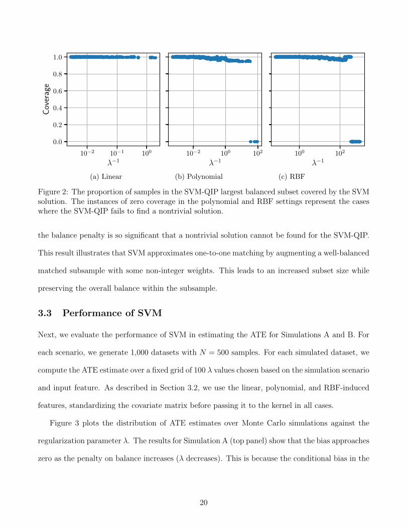
Interestingly, the coverage plots in Figure 2 show that even when the objective values of the

two methods are divergent, the SVM solution still predominantly covers the SVM-QIP solution.

The regions with zero coverage in the polynomial and RBF settings correspond to instances where

19

10−2 10−1 100

λ−1

0.0

0.2

0.4

0.6

0.8

1.0

Cov

erag

e

10−2 100 102

λ−1100 102

λ−1

(a) Linear (b) Polynomial (c) RBF

Figure 2: The proportion of samples in the SVM-QIP largest balanced subset covered by the SVMsolution. The instances of zero coverage in the polynomial and RBF settings represent the caseswhere the SVM-QIP fails to find a nontrivial solution.

the balance penalty is so significant that a nontrivial solution cannot be found for the SVM-QIP.

This result illustrates that SVM approximates one-to-one matching by augmenting a well-balanced

matched subsample with some non-integer weights. This leads to an increased subset size while

preserving the overall balance within the subsample.

3.3 Performance of SVM

Next, we evaluate the performance of SVM in estimating the ATE for Simulations A and B. For

each scenario, we generate 1,000 datasets with N = 500 samples. For each simulated dataset, we

compute the ATE estimate over a fixed grid of 100 λ values chosen based on the simulation scenario

and input feature. As described in Section 3.2, we use the linear, polynomial, and RBF-induced

features, standardizing the covariate matrix before passing it to the kernel in all cases.

Figure 3 plots the distribution of ATE estimates over Monte Carlo simulations against the

regularization parameter λ. The results for Simulation A (top panel) show that the bias approaches

zero as the penalty on balance increases (λ decreases). This is because the conditional bias in the

20

10−2 100

λ−1

−0.6

−0.5

−0.4

−0.3

−0.2

−0.1

AT

E

10−2 100

λ−1

Simulation A

100 102

λ−1

10−2 100

λ−1

−5

0

5

10

15

20

AT

E

10−2 100 102

λ−1

Simulation B

100 102

λ−1

(a) Linear (b) Polynomial (c) RBF

Figure 3: ATE estimates for Simulations A (top) and B (bottom) over the SVM regularizationpath. The boxplots represent the distribution of the ATE estimates over Monte Carlo simulations.The red dashed line corresponds to the true ATE.

estimate under the outcome model for Simulation A is given by,

E[τ − τ | X1:N , T1:N ] = γ>(

N∑i=1

αiTiXi

).

This implies that all bias comes from prognostic score imbalance. This quantity becomes the

smallest when minimizing∥∥∥∑N

i=1 αiTiXi

∥∥∥, which is controlled by the regularization parameter λ

in the SVM dual objective under the linear setting. Note that this quantity is also small under

21

both the polynomial and RBF input features.

We also find that under all three settings, there is relatively little change in the variance of the

estimates along most of the path, suggesting that the variance gained from trimming the sample

is counteracted by the variance decreased from correcting for heteroscedasticity. The exception to

this observation occurs at the beginning of the linear case, where the reduction in bias also reduces

the variance, and at the end of the RBF path, where the amount of trimming is so substantial

relative to the balance gained that the variance increases.

For Simulation B (bottom panel), the bias decreases as the penalty on balance increases.

However, due to misspecification, nonlinearity, and treatment effect heterogeneity in the outcome

model, the bias never decays to zero as shown in Section 2.6. We also find that the SVM with

linear kernel can reduce bias as well as the other kernels, suggesting that SVM is robust to

misspecification and nonlinearity in the outcome model. Similar to Simulation A, we observe

relatively small changes in the variance as the constraint on balance increases, except at the end

of the RBF path where there is substantial sample pruning.

3.4 Comparison with Other Methods

Next, we compare the performance of SVM with that of other methods. Our results below show

that the performance of SVM is comparable to that of related state-of-the-art covariate balancing

methods available in the literature. In particular, we consider kernel optimal matching (KOM;

Kallus et al., 2021), kernel covariate balancing (KCB; Wong and Chan, 2018), cardinality matching

(CARD; Zubizarreta et al., 2014), and inverse propensity score weighting (IPW) based on logistic

regression (GLM) and random forest (RFRST), both of which were used in the original simulation

study by Lee et al. (2010). For SVM, we compute solutions using λ−1 = 0.42, λ−1 = 0.10, and

λ−1 = 2.60 for Simulation A under the linear, polynomial, and RBF settings, respectively. For

Simulation B, we use λ−1 = 1.07, λ−1 = 1.92, and λ−1 = 10.48. These values are taken from the

22

SVM KOM KCB CARD GLM RFRST

Method

−0.55

−0.50

−0.45

−0.40

−0.35

−0.30

−0.25

−0.20

AT

E

Linear

Polynomial

RBF

SVM KOM KCB CARD GLM RFRST

Method

0

10

20

30

40

50

60

(a) Simulation A (b) Simulation B

Figure 4: Boxplots for ATE estimates for Simulations A (left) and B (right). The hatch patterndenotes the input feature (Linear, Polynomial, or RBF) — kernel optimal matching (KOM; Kalluset al., 2021), kernel covariate balancing (KCB; Wong and Chan, 2018), cardinality matching(CARD; Zubizarreta et al., 2014), and IPW with propensity score modeling via logistic regression(GLM) and random forest (RFRST). The red dashed line corresponds to the true ATE.

grid of λ values used in the simulation based on visual inspection of the path plots in Figure 3

around where the estimate curve flattens out.

For KOM, we compute weights under the linear, polynomial, and RBF settings described

earlier with the default settings for the provided code. For KCB, we compute weights using the

RBF kernel and use its default settings. While KCB allows for other kernel functions, it was

originally designed for the use of RBF and Sobolev kernels. We find its results to be poor when

using the linear and polynomial features. For CARD, we used a threshold of 0.01 and 0.1 times

the standardized difference-in-means for the linear- and polynomial-induced features, respectively,

and we set the search time for the algorithm to 3 minutes. For GLM and RFRST, we used the

linear-induced features and the default algorithm settings described in Lee et al. (2010).

Figure 4 plots the distributions of the effect estimates over 1,000 simulated datasets for both

23

scenarios. Simulation A (left panel) shows comparable performance across all methods, with SVM

and KOM having the best performance in terms of both bias and variance. In particular, SVM

achieves near zero bias under all three input features. The results for KCB show that it performs

slightly worse in comparison to the other kernel methods, with greater bias and variance under

the RBF setting.

The results for CARD show near identical performance with SVM under the linear setting,

however results under the polynomial setting are notably worse. The reason for this comes from

the choice of balance threshold, which was set to 0.1 times the standardized difference-in-means

of the input feature matrix. Although decreasing the scalar below 0.1 would lead to a more

balanced matching, we found that algorithm was unable to consistently find a solution for all

datasets with scalar multiples smaller than 0.1. This result highlights the main issue with defining

balance dimension-by-dimension, which makes it difficult to enforce small overall balance without

information on the underlying geometry of the data. Lastly, the propensity score methods show

the worst performance. This is somewhat expected as the true propensity score model is more

complicated than the true outcome model under this simulation setting.

We note that further reduction in the variance of the SVM solution while preserving bias is

likely possible with a more principled method of choosing the solution for each simulated dataset.

In general, a value of λ that works well for one dataset may not work for another. A better

approach would examine estimates over the path and balance-sample size curves for each dataset

individually. Nevertheless, our heuristic procedure to selecting a solution produced high-quality

results.

The results for Simulation B (right panel) show a slightly more varying performance across

methods. Amongst the kernel methods, we find that KOM has the best performance under the

polynomial and RBF settings, achieving near zero bias under these scenarios, while SVM has

the best performance under the linear setting. The discrepancy under the linear setting is due

24

to misspecification, which leads to a poor regularization parameter choice and consequently poor

balance and bias under the KOM procedure.

We also find that SVM is unable to drive the bias to zero, which is due to the treatment effect

heterogeneity in the outcome model. As discussed in Section 2.6, SVM ignores the second term in

the conditional bias decomposition in Eqn (15), which is zero under a constant additive treatment

effect in Simulation A but is nonzero in Simulation B. In contrast, KOM targets both bias terms

in its formulation, which leads to greater bias reduction.

In comparison to the other kernel methods, KCB has comparable bias to SVM but greater

variance. For CARD, we observe comparable results to SVM under the linear setting, but worse

performance under the polynomial setting due to the reasons mentioned above. Lastly, we find

mixed results between the two propensity score methods. Logistic regression (GLM) has the worst

performance while Random forest (RFRST) exhibits the second best performance. This result is

likely due to the simple structure of the true propensity score model, whose nonlinearity can only

be accurately modeled by RFRST.

4 Empirical Application: Right Heart Catheterization Study

In this section, we apply the proposed methodology to the right heart catheterization (RHC) data

set originally analyzed in Connors et al. (1996). This observational data set was used to study the

effectiveness of right heart catheterization, a diagnostic procedure, for critically ill patients. The

key result from the study was that after adjusting for a large number of pre-treatment covariates,

right heart catheterization appeared to reduce survival rates. This finding contradicts the existing

medical perception that the procedure is beneficial.

25

4.1 Data and Methods

The data set consists of 5,735 patients, with 2,184 of them assigned to the treatment group and

3,551 assigned to the control group. For each patient, we observe the treatment status, which

indicates whether or not he/she received catheterization within 24 hours of hospital admission.

The outcome variable represents death within 30 days. Finally, the dataset contains a total of

72 pre-treatment covariates that are thought to be related to the decision to perform right heart

catheterization. These variables include background information about the patient, such as age,

sex, and race, indicator variables for primary/secondary diseases and comorbidities, and various

measurements from medical test results.

We compute the full SVM regularization paths under the linear, polynomial, and RBF settings

described in Section 3.1. For the polynomial features, we exclude all trivial interactions (e.g.,

interactions between categories of the same categorical variable) and squares of binary-valued

covariates. We also compute the KOM weights under all three settings, the KCB weights under

the RBF setting, and the CARD weights under the linear and polynomial settings with a threshold

set to 0.1 times the standardized difference-in-means.

4.2 Results

Figure 5 plots the ATE estimates over the SVM regularization paths with the pointwise 95%

confidence intervals based on the weighted Neyman variance estimator (Imbens and Rubin, 2015,

Chapter 19). The horizontal axis represents the normed difference-in-means within the weighted

subset as a covariate balance measure. For all three settings, we find that the estimated ATE

slightly increases as the weighted subset becomes more balanced, supporting the results originally

reported in Connors et al. (1996) that right heart catheterization decreased survival rates.

Figure 6 illustrates the trade-off between the balance measure (the normed difference-in-means

in covariates within the weighted subset) and effective subset size, as the balance-sample size

26

0.0 0.2 0.4 0.6

0.00

0.04

0.08

0.12

AT

E

0 1 2

Normed difference-in-means0.02 0.04

(a) Linear (b) Polynomial (c) RBF

Figure 5: ATE estimates for the RHC data over the SVM regularization path. The horizontalaxis represents the normed difference-in-means in covariates within the weighted subset. The solidblue line denotes the average estimate, and the solid gray background denotes the pointwise 95%confidence intervals.

3500 3750 4000 4250

0.0

0.2

0.4

0.6

Nor

med

diff

eren

ce-i

n-m

eans

1000 2000 3000 4000

Effective sample size

0.0

0.5

1.0

1.5

2.0

2.5

1000 2000 3000 4000

0.01

0.02

0.03

0.04

0.05

(a) Linear (b) Polynomial (c) RBF

Figure 6: Trade-off between balance and effective sample size. The black dashed-line indicates theestimated elbow point.

frontier. Such graphs can be useful to researchers in selecting a solution along the regularization

path for estimating the ATE. Across all cases, we achieve a good amount of balance improvement

once the data set is pruned to about 3,500, which occurs around where the trade-off between

subset size balance becomes less favorable.

We also examine differences in dimension-by-dimension balance between SVM and CARD and

27

between SVM and KOM under the linear and polynomial settings. We do not conduct such a

comparison for RBF, which is infinite dimensional. Here, we consider four different SVM solutions:

the largest subset size solution whose standardized difference-in-means in covariates was below 0.1

for all dimensions, the solution whose effective sample size was nearest the subset size for the other

method, the solution whose normed difference-in-means in covariates was closest to that of the

other method, and the solution occurring at the kneedle estimate for the elbow of the balance-

weight sum curve. We take the minimum-balance solution when no elbow exists, as in the linear

case. The effective sample size is computed according to the following Kish’s formula:

Ne =

(∑i∈T αi

)2∑i∈T α

2i

+

(∑i∈C αi

)2∑i∈C α

2i

. (21)

Figure 7 presents the covariate balance comparisons between SVM and CARD for both linear

and polynomial settings. Comparing against the small difference-in-means solution (leftmost col-

umn) for which the standardized difference-in-means for all covariates are below 0.1, CARD retains

more observations in its selected subset, but SVM achieves a better covariate balance than CARD

for most dimensions although there are some large imbalances. This is expected because SVM

minimizes the overall covariate imbalance without a constraint on each dimension as in CARD.

We observe a similar result when comparing CARD with the SVM solutions based on the closest

effective sample size solution (left-middle) and the closest normed difference-in-means solution

(right-middle). It is notable that the latter generally achieves a better covariate balance while re-

taining more observations than CARD. Finally, the results for the elbow SVM solution (rightmost

column) show that tight balance is attainable with a moderate amount of sample pruning, with

near exact balance in the linear setting. This level of covariate balance is difficult to achieve with

CARD due to the infeasibility of optimization particularly in high dimensional settings.

Figure 8 shows the dimensional balance comparisons for the KOM solution against the SVM

28

0.0 0.1 0.2

SVM (Ne = 3830)

0.0

0.1

0.2

CA

RD

(Ne

=41

74)

0.0 0.1 0.2

SVM (Ne = 4186)0.0 0.1 0.2

SVM (Ne = 4367)0.0 0.1 0.2

SVM (Ne = 3442)

0.0 0.1 0.2

SVM (Ne = 3777)

0.0

0.1

0.2

CA

RD

(Ne

=40

84)

0.0 0.1 0.2

SVM (Ne = 4071)0.0 0.1 0.2

SVM (Ne = 4304)0.0 0.1 0.2

SVM (Ne = 3325)

(a) Smalldifference-

in-means

(b) Closest effec-tive

sample size

(c) Closest normeddifference-in-means

(d) Elbow

Figure 7: Comparison of covariate standardized difference-in-means between SVM and cardinalitymatching (CARD) under the linear (top) and polynomial (bottom) settings with different SVMsolutions: (a) standardized difference-in-means less than 0.1 in all covariates, (b) effective samplesize closest to that of CARD, (c) normed difference-in-means closest to that of CARD, and (d)elbow of the regularization path. The effective sample size for each method is given as Ne in theparentheses. Note that darker areas correspond to higher concentrations of points.

solution. Here, we see that under the linear setting, KOM retains significantly more units than

the SVM solution while attaining the same balance. This is due to the∑

i αWi = 0 constraint

of SVM, which encourages the selected subset to have a roughly equal proportion of treated and

control units, while the KOM solution allows the resulting subset to be more imbalanced. Under

the polynomial setting, however, we find that SVM retains significantly more units than KOM

while achieving a similar degree of covariate balance, which is likely due to poor regularization

parameter choice by the KOM algorithm.

Lastly, we compare the point estimates of the ATE, the weighted Neyman standard error, and

29

10−7 10−6 10−5 10−4

SVM (Ne = 3443)

10−7

10−6

10−5

10−4

KO

M(N

e=

4159

)

0.00 0.04 0.08

SVM (Ne = 3356)

0.00

0.04

0.08

KO

M(N

e=

1623

)

(a) Linear (b) Polynomial

Figure 8: Comparison of covariate standardized difference-in-means between SVM and kerneloptimal matching (KOM) under the linear (left) and polynomial (right) settings.

the effective sample size for SVM, CARD (with linear and polynomial), KOM, and KCB (with

RBF) in Table 1. We considered three different solutions from the SVM path: SVMimbalance, which

corresponds to the initial solution for which the balance constraint is most relaxed and αi = 1,

i ∈ T , SVMbalance, which corresponds to the most regularized solution with the best covariate

balance on the path, and SVMelbow, which corresponds to the solution occurring at the elbow of

the balance-weight sum curves shown in Figure 6.

The results show that SVM leads to a positive estimate in all cases, which agrees with the

original finding reported in Connors et al. (1996). We also find that the three SVM solutions differ

most significantly in their standard errors, which increases as the constraint on balance becomes

stronger and the subset is more pruned, as shown in the effective sample size column. In particular,

the heavily balanced SVMbalance solution under the RBF setting leads to a 95% confidence interval

which overlaps with zero. This is in contrast with the less balanced SVMelbow solution, which

has both a larger effect estimate and smaller confidence interval. This result demonstrates the

necessity of computing the regularization path so that researchers may avoid low-quality solutions

due to poor parameter choice.

30

Feature Method Estimate Standard error Effective sample size

Linear

SVMbalance 0.0615 0.0148 3442SVMelbow — — —SVMimbalance 0.0479 0.0132 4367CARD 0.0335 0.0138 4174KOM 0.0656 0.0147 4159

Polynomial

SVMbalance 0.0634 0.0279 1087SVMelbow 0.0588 0.0154 3325SVMimbalance 0.0541 0.0135 4375CARD 0.0313 0.0139 4084KOM 0.0452 0.0251 1623

RBF

SVMbalance 0.0518 0.0289 1123SVMelbow 0.0527 0.0148 3444SVMimbalance 0.0474 0.0132 4378KCB 0.0337 0.0173 3306KOM 0.0582 0.0166 4185

Table 1: The estimated effect of right heart catheterization on death within 30 days after treat-ment. We compare the results based on cardinality matching (CARD) and Kernel Optimal Match-ing (KOM) with those based on three SVM solutions – the solution with the best covariate balanceon the regularization path in terms of normed difference-in-means (SVMbalance), the elbow solution(SVMelbow), and the solution with the worst covariate balance on the path (SVMimbalance).

Comparing against other methods, we observe that KOM yields greater estimates of positive

effects with comparable standard errors in the linear and RBF settings. However, under the

polynomial setting, the standard error is much larger and the sample is significantly more pruned

than the modestly balanced SVMelbow solution. Both CARD and KCB produce smaller positive

effect estimates, with the standard error for KCB leading to a 95% confidence interval which

overlaps with zero.

5 Concluding Remarks

In this paper, we show how support vector machines (SVMs) can be used to compute covariate

balancing weights and estimate causal effects. We establish a number of interpretations of SVM as

a covariate balancing procedure. First, the SVM dual problem computes weights which minimize

31

the MMD while simultaneously maximizing effective sample size. Second, the SVM dual problem

can be viewed as a continuous relaxation of the largest balanced subset problem. Lastly, similar to

existing kernel balancing methods, SVM weights minimize the worst-case bias due to prognostic

score imbalance. Additionally, path algorithms can be used to compute the entire set of SVM

solutions as the regularization parameter varies, which constitutes a balance-sample size frontier.

Our work suggests several possible directions for future research. On the algorithmic side, a

disadvantage of the proposed methodology is that it encourages roughly equal effective number of

treated and control units in the optimal subset, which can lead to unnecessary sample pruning.

One could use weighted SVM (Lin and Wang, 2002) to address this problem, but existing path

algorithms are applicable only to unweighted SVM. On the theoretical side, our results suggest

a fundamental connection between the support vectors and the set of overlap. Steinwart (2004)

shows that the fraction of support vectors for a variant of the SVM discussed here asymptotically

approaches the measure of this overlap set, suggesting that SVM may be used to develop a

statistical test for the overlap assumption.

References

Athey, S., Imbens, G. W., and Wager, S. (2018). Approximate residual balancing: debiased

inference of average treatment effects in high dimensions. Journal of the Royal Statistical Society,

Series B, Methodological , 80(4), 597–623.

Chan, K. C. G., Yam, S. C. P., and Zhang, Z. (2016). Globally efficient nonparametric inference

of average treatment effects by empirical balancing calibration weighting. Journal of the Royal

Statistical Society, Series B, Methodological , 78, 673–700.

Connors, A. F., Speroff, T., Dawson, N. V., Thomas, C., Harrell, F. E., Wagner, D., Desbiens,

32

N., Goldman, L., Wu, A. W., Califf, R. M., et al. (1996). The effectiveness of right heart

catheterization in the initial care of critically iii patients. Jama, 276(11), 889–897.

Cortes, C. and Vapnik, V. (1995). Support-vector networks. Machine learning , 20(3), 273–297.

Dinkelbach, W. (1967). On nonlinear fractional programming. Management science, 13(7), 492–

498.

Ghosh, D. (2018). Relaxed covariate overlap and margin-based causal effect estimation. Statistics

in Medicine, 37(28), 4252–4265.

Gretton, A., Borgwardt, K., Rasch, M., Scholkopf, B., and Smola, A. J. (2007a). A kernel method

for the two-sample-problem. In Advances in neural information processing systems , pages 513–

520.

Gretton, A., Fukumizu, K., Teo, C., Song, L., Scholkopf, B., and Smola, A. (2007b). A kernel

statistical test of independence. Advances in neural information processing systems , 20, 585–

592.

Gretton, A., Borgwardt, K. M., Rasch, M. J., Scholkopf, B., and Smola, A. (2012). A kernel

two-sample test. The Journal of Machine Learning Research, 13(1), 723–773.

Gurobi Optimization, L. (2020). Gurobi optimizer reference manual.

Hainmueller, J. (2012). Entropy balancing for causal effects: A multivariate reweighting method

to produce balanced samples in observational studies. Political analysis , pages 25–46.

Hansen, B. B. (2008). The prognostic analogue of the propensity score. Biometrika, 95(2),

481–488.

Hastie, T., Rosset, S., Tibshirani, R., and Zhu, J. (2004). The entire regularization path for the

support vector machine. Journal of Machine Learning Research, 5(Oct), 1391–1415.

33

Hazlett, C. (2020). Kernel balancing: A flexible non-parametric weighting procedure for estimating

causal effects. Statistica Sinica, 30(3), 1155–1189.

Ho, D. E., Imai, K., King, G., and Stuart, E. A. (2007). Matching as nonparametric preprocessing

for reducing model dependence in parametric causal inference. Political Analysis , 15(3), 199–

236.

Imai, K. and Ratkovic, M. (2014). Covariate balancing propensity score. Journal of the Royal

Statistical Society, Series B (Statistical Methodology), 76(1), 243–263.

Imbens, G. W. and Rubin, D. B. (2015). Causal inference in statistics, social, and biomedical

sciences . Cambridge University Press.

Kallus, N. (2020). Generalized optimal matching methods for causal inference. Journal of Machine

Learning Research, 21(62), 1–54.

Kallus, N., Pennicooke, B., and Santacatterina, M. (2018). More robust estimation of sample

average treatment effects using kernel optimal matching in an observational study of spine

surgical interventions. arXiv preprint arXiv:1811.04274 .

Kallus, N., Pennicooke, B., and Santacatterina, M. (2021). More robust estimation of average

treatment effects using kernel optimal matching in an observational study of spine surgical

interventions. Statistics in Medicine.

King, G. and Zeng, L. (2006). The dangers of extreme counterfactuals. Political Analysis , 14(2),

131–159.

King, G., Lucas, C., and Nielsen, R. A. (2017). The balance-sample size frontier in matching

methods for causal inference. American Journal of Political Science, 61(2), 473–489.

34

Lee, B. K., Lessler, J., and Stuart, E. A. (2010). Improving propensity score weighting using

machine learning. Statistics in medicine, 29(3), 337–346.

Li, F., Morgan, K. L., and Zaslavsky, A. M. (2018). Balancing covariates via propensity score

weighting. Journal of the American Statistical Association, 113(521), 390–400.

Lin, C.-F. and Wang, S.-D. (2002). Fuzzy support vector machines. IEEE transactions on neural

networks , 13(2), 464–471.

Lunceford, J. K. and Davidian, M. (2004). Stratification and weighting via the propensity score

in estimation of causal treatment effects: A comparative study. Statistics in Medicine, 23(19),

2937–2960.

Ning, Y., Peng, S., and Imai, K. (2020). Robust estimation of causal effects via high-dimensional

covariate balancing propensity score. Biometrika, 107(3), 533–554.

Ratkovic, M. (2014). Balancing within the margin: Causal effect estimation with support vec-

tor machines. Department of Politics, Princeton University, Princeton, NJ , page available at

https://www.princeton.edu/~ratkovic/public/BinMatchSVM.pdf.

Rubin, D. B. (1990). Comments on “On the application of probability theory to agricultural

experiments. Essay on principles. Section 9” by J. Splawa-Neyman translated from the Polish

and edited by D. M. Dabrowska and T. P. Speed. Statistical Science, 5, 472–480.

Rubin, D. B. (2006). Matched Sampling for Causal Effects . Cambridge University Press, Cam-

bridge.

Schaible, S. (1976). Fractional programming. ii, on dinkelbach’s algorithm. Management science,

22(8), 868–873.

35

Scholkopf, B., Smola, A. J., Bach, F., et al. (2002). Learning with kernels: support vector machines,

regularization, optimization, and beyond . MIT press.

Sentelle, C., Anagnostopoulos, G., and Georgiopoulos, M. (2016). A simple method for solving

the svm regularization path for semidefinite kernels. IEEE transactions on neural networks and

learning systems , 27(4), 709.

Setoguchi, S., Schneeweiss, S., Brookhart, M. A., Glynn, R. J., and Cook, E. F. (2008). Evaluating

uses of data mining techniques in propensity score estimation: a simulation study. Pharma-

coepidemiology and drug safety , 17(6), 546–555.

Sriperumbudur, B. K. (2011). Mixture density estimation via hilbert space embedding of measures.

In 2011 IEEE International Symposium on Information Theory Proceedings , pages 1027–1030.

IEEE.

Sriperumbudur, B. K., Gretton, A., Fukumizu, K., Scholkopf, B., and Lanckriet, G. R. (2010).

Hilbert space embeddings and metrics on probability measures. The Journal of Machine Learn-

ing Research, 11, 1517–1561.

Sriperumbudur, B. K., Fukumizu, K., Gretton, A., Scholkopf, B., Lanckriet, G. R., et al. (2012).

On the empirical estimation of integral probability metrics. Electronic Journal of Statistics , 6,

1550–1599.

Steinwart, I. (2004). Sparseness of support vector machines—some asymptotically sharp bounds.

In Advances in Neural Information Processing Systems , pages 1069–1076.

Stuart, E. A. (2010). Matching methods for causal inference: A review and a look forward.

Statistical Science, 25(1), 1–21.

Tan, Z. (2010). Bounded, efficient and doubly robust estimation with inverse weighting.

Biometrika, 97(3), 661–682.

36

Tan, Z. (2020). Regularized calibrated estimation of propensity scores with model misspecification

and high-dimensional data. Biometrika, 107(1), 137–158.

Wong, R. K. and Chan, K. C. G. (2018). Kernel-based covariate functional balancing for obser-

vational studies. Biometrika, 105(1), 199–213.

Zhao, Q. (2019). Covariate balancing propensity score by tailored loss functions. Annals of

Statistics , 47(2), 965–993.

Zhu, Y., Savage, J. S., and Ghosh, D. (2018). A kernel-based metric for balance assessment.

Journal of causal inference, 6(2).

Zubizarreta, J. R. (2015). Stable weights that balance covariates for estimation with incomplete

outcome data. Journal of the American Statistical Association, 110(511), 910–922.

Zubizarreta, J. R., Paredes, R. D., Rosenbaum, P. R., et al. (2014). Matching for balance, pairing

for heterogeneity in an observational study of the effectiveness of for-profit and not-for-profit

high schools in chile. The Annals of Applied Statistics , 8(1), 204–231.

37

Supplementary Appendix for “Estimating Average Treatment Effects

with Support Vector Machines”

A Proof of Theorem 1

We prove this theorem by establishing several equivalent reformulations of the SVM dual problem.

By equivalence, we mean that these problems differ from one another only in the scaling of

the regularization parameter, implying that their regularization paths consist of the same set of

solutions. More formally, given two optimization problems P1 and P2, we say that P1 and P2 are

equivalent if a solution α∗1 for P1 can be used to construct a solution for P2.

Denote the SVM weight set

ASVM =

{α ∈ RN : 0 � α. � 1,

∑i∈T

αi =∑j∈C

αj

},

and consider a rescaled version of the SVM dual given in Eqn (4), which we label as P1:

minα

α>Qα− µ1>α.

s.t. α ∈ ASVM

(P1)

Note that for a given λ and solution α∗ to the original problem defined in Eqn (4) under λ, α∗

is also a solution to the rescaled problem P1 under µ = 2λ. This establishes equivalence between

these two problems.

We begin by proving the following lemma, which allows us to replace the squared seminorm

term α>Qα with√α>Qα to obtain the problem

minα

√α>Qα− ν1>α.

s.t. α ∈ ASVM

(P2)

Lemma 1 The problems given in Eqn (P1) and Eqn (P2) are equivalent.

Proof This result follows from the strong duality of the SVM dual problem, which allows us to

form the following equivalent problem in which the penalized term 1>α is replaced with a hard

constraint with threshold ε:minα

α>Qα.

s.t. α ∈ ASVM

1>α ≥ ε

(P3)

38

The solution to Eqn (P3) is unchanged whether we minimize α>Qα or√α>Qα, so the problem

minα

√α>Qα

s.t. α ∈ ASVM

1>α ≥ ε

is identical to Eqn (P3). By strong duality, we can again enforce the hard constraint on the

term 1>α through a penalized term with new regularization parameter, which establishes the

equivalence between Eqn (P1) and Eqn (P2). 2

Next, we consider the fractional program

minα

√α>Qα

1>α/2.

s.t. α ∈ ASVM

(P4)

The following lemma connects Eqn (P4) to the reformulated SVM problem given in Eqn (P2)

through Dinkelbach’s method (Dinkelbach, 1967; Schaible, 1976):

Lemma 2 (Dinkelbach, 1967, Theorem 1) Suppose α∗ ∈ ASVM and α∗ 6= 0. Then

q∗ =

√α>∗Qα∗

1>α∗/2= minα∈ASVM

√α>Qα

1>α/2

if, and only if

minα∈ASVM

√α>Qα− q∗

21>α =

√α>∗Qα∗ −

q∗2

1>α∗ = 0.

Thus, the solution to the rescaled SVM dual problem defined in Eqn (P2) under ν = q∗/2

minimizes the fractional program given in Eqn (P4). Finally, we consider the MMD minimization

problem defined in Eqn (11),

minα

√α>Qα.

s.t. α ∈ Asimplex

(P5)

The following lemma establishes equivalence between Eqn (P4) and Eqn (P5) under the proper

renormalization of the fractional program solution.

Lemma 3 Assume any solution α∗ to (P4) is such that α∗ 6= 0. Then the problems (P4) and

(P5) are equivalent.

Proof Let α4 6= 0 and α5 be solutions to problems defined in Eqn (P4) and Eqn (P5), respec-

tively, and consider the vector-valued function f : ASVM \ 0 7→ Asimplex, f(α) = α/(1>α/2),

39

which normalizes the weights in the treated and control groups to each sum to 1. First note that

since Asimplex ⊂ ASVM \ 0, α5 is feasible for Eqn (P4). Then by optimality of α4, we have√α>4Qα4

1>α4/2≤√α>5Qα5

1>α5/2=√α>5Qα5.

Next, note that f(α4) is feasible for Eqn (P5). Then by optimality of α5, we have

√α>5Qα5 ≤

√f(α4)>Qf(α4) =

√α>4Qα4

1>α4/2.

In order for both of these inequalities to be true, we must have√α>4Qα4

1>α4/2=

√α>5Qα5

1>α5/2=√α>5Qα5.

2

Note that the assumption α 6= 0 in Lemma 2 and Lemma 3 holds when ν ≥ q∗/2, provided that

the data does not consist of samples all belonging to the same class. To see this, note that when

ν = q∗/2, both α = 0 and any scaled version of the MMD-minimizing solution, α = cα∗, c > 0,

lead to an objective value of 0 in Eqn(P2). Then since Eqn (P2) is a strictly monotonically

decreasing function of ν, we must have α 6= 0 for ν > q∗/2. Now since the regularization path

defined in this work only considers ν ≥ q∗/2, we may safely assume α 6= 0.

We are now ready to prove Theorem 1. Part (i): Lemma 1 establishes equivalence between the

regularization paths for the rescaled SVM dual defined in Eqn (P1) and Eqn (P2). In addition,

Lemma 2 establishes the existence of ν∗ such that the solution to Eqn (P2) under ν∗ is also a

solution to Eqn (P4). Then, it follows that there exists λ∗ such that the solution to the rescaled

SVM dual problem under λ∗ minimizes Eqn (P4). Finally, recall that Lemma 3 establishes that the

minimizing solution to Eqn (P4) is also a solution to the weighted MMD minimization problem.

Therefore, there exists λ∗ such that the solution to the SVM dual under λ∗ minimizes the weighted

MMD. Part (ii): The proof follows from Schaible (1976, Lemma 3).

B Relation to Cardinality Matching and Stable Balancing

Weights

Cardinality matching is an optimization procedure that maximizes the number of matches subject

to a set of covariate balance constraints. The optimization problem for cardinality matching is

40

given by,

minmij

∑i∈T

∑j∈C

mij

s.t. |∑i∈T

∑j∈C

mij[fb(Xid)− fb(Xjd)]| ≤ εdb∑i∈T

∑j∈C

mij, d = 1, . . . , D, b = 1, . . . , B∑j∈C

mij ≤ 1, i ∈ T∑i∈T

mij ≤ 1, j ∈ C

mij ∈ {0, 1}, i ∈ T , j ∈ C,

(22)

where mij are selection variables indicating whether treated unit i is matched to control unit j,

Xid denotes the dth element of covariate vector Xi, fb is an arbitrary function of the covariates

specifying each of the B balance conditions, and εdb is a tolerance selected by a researcher. Com-

mon choices for fb are the first- and second-order moments, and εdb is typically set to a scalar

multiple of the corresponding standardized difference-in-means.

To establish the connection between SVM and cardinality matching, we first note that car-

dinality matching need not be formulated as a matched pair optimization problem. In fact, the

balance constraints between pairs, as formulated in Eqn (22), are equivalent to those between

the treatment and control groups in the selected subsample. Similarly, the one-to-one matching

constraints are equivalent to restricting the number of treated and control units in the selected

subsample to be equal. Therefore, defining the indicator variable αi for selection into the optimal

subset, we can rewrite the optimization problem for cardinality matching as,

minα

1

2

N∑i=1

αi

s.t. |∑i∈T

αifb(Xid)−∑j∈C

αjfb(Xjd)| ≤1

2εdb

N∑i=1

αi, d = 1, . . . , D, b = 1, . . . , B

N∑i=0

αiWi = 0,

αi ∈ {0, 1}, i = 1, . . . , N.

(23)

Comparing this problem to the SVM dual defined in Eqn (4), we see two differences. First,

cardinality matching restricts αi to be integer-valued, while SVM allows for αi to be continuous.

Second, balance in the optimal subset is enforced differently in each method. Cardinality matching

imposes covariate-specific balance by bounding each dimension’s difference-in-means, while SVM

41

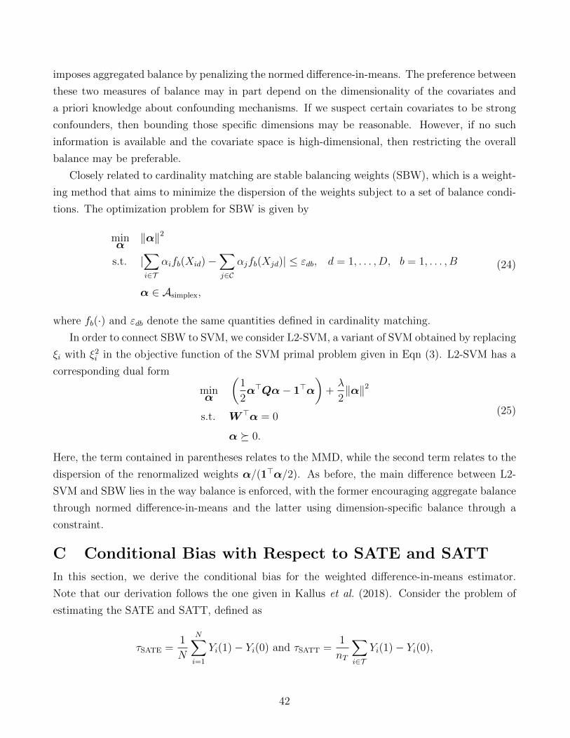
imposes aggregated balance by penalizing the normed difference-in-means. The preference between

these two measures of balance may in part depend on the dimensionality of the covariates and

a priori knowledge about confounding mechanisms. If we suspect certain covariates to be strong

confounders, then bounding those specific dimensions may be reasonable. However, if no such

information is available and the covariate space is high-dimensional, then restricting the overall

balance may be preferable.

Closely related to cardinality matching are stable balancing weights (SBW), which is a weight-

ing method that aims to minimize the dispersion of the weights subject to a set of balance condi-

tions. The optimization problem for SBW is given by

minα

‖α‖2

s.t. |∑i∈T

αifb(Xid)−∑j∈C

αjfb(Xjd)| ≤ εdb, d = 1, . . . , D, b = 1, . . . , B

α ∈ Asimplex,

(24)

where fb(·) and εdb denote the same quantities defined in cardinality matching.

In order to connect SBW to SVM, we consider L2-SVM, a variant of SVM obtained by replacing

ξi with ξ2i in the objective function of the SVM primal problem given in Eqn (3). L2-SVM has a

corresponding dual form

minα

(1

2α>Qα− 1>α

)+λ

2‖α‖2

s.t. W>α = 0

α � 0.

(25)

Here, the term contained in parentheses relates to the MMD, while the second term relates to the

dispersion of the renormalized weights α/(1>α/2). As before, the main difference between L2-

SVM and SBW lies in the way balance is enforced, with the former encouraging aggregate balance

through normed difference-in-means and the latter using dimension-specific balance through a

constraint.

C Conditional Bias with Respect to SATE and SATT

In this section, we derive the conditional bias for the weighted difference-in-means estimator.

Note that our derivation follows the one given in Kallus et al. (2018). Consider the problem of

estimating the SATE and SATT, defined as

τSATE =1

N

N∑i=1

Yi(1)− Yi(0) and τSATT =1

nT

∑i∈T

Yi(1)− Yi(0),

42

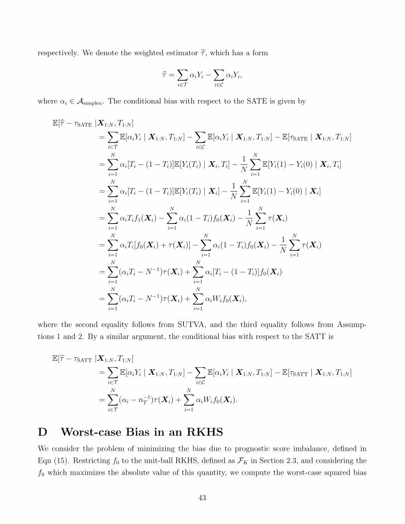
respectively. We denote the weighted estimator τ , which has a form

τ =∑i∈T

αiYi −∑i∈C

αiYi,

where αi ∈ Asimplex. The conditional bias with respect to the SATE is given by

E[τ − τSATE |X1:N , T1:N ]

=∑i∈T

E[αiYi |X1:N , T1:N ]−∑i∈C

E[αiYi |X1:N , T1:N ]− E[τSATE |X1:N , T1:N ]

=N∑i=1

αi[Ti − (1− Ti)]E[Yi(Ti) |Xi, Ti]−1

N

N∑i=1

E[Yi(1)− Yi(0) |Xi, Ti]

=N∑i=1

αi[Ti − (1− Ti)]E[Yi(Ti) |Xi]−1

N

N∑i=1

E[Yi(1)− Yi(0) |Xi]

=N∑i=1

αiTif1(Xi)−N∑i=1

αi(1− Ti)f0(Xi)−1

N

N∑i=1

τ(Xi)

=N∑i=1

αiTi[f0(Xi) + τ(Xi)]−N∑i=1

αi(1− Ti)f0(Xi)−1

N

N∑i=1

τ(Xi)

=N∑i=1

(αiTi −N−1)τ(Xi) +N∑i=1

αi[Ti − (1− Ti)]f0(Xi)

=N∑i=1

(αiTi −N−1)τ(Xi) +N∑i=1

αiWif0(Xi),

where the second equality follows from SUTVA, and the third equality follows from Assump-

tions 1 and 2. By a similar argument, the conditional bias with respect to the SATT is

E[τ − τSATT |X1:N , T1:N ]

=∑i∈T

E[αiYi |X1:N , T1:N ]−∑i∈C

E[αiYi |X1:N , T1:N ]− E[τSATT |X1:N , T1:N ]

=N∑i∈T

(αi − n−1T )τ(Xi) +N∑i=1

αiWif0(Xi).

D Worst-case Bias in an RKHS

We consider the problem of minimizing the bias due to prognostic score imbalance, defined in

Eqn (15). Restricting f0 to the unit-ball RKHS, defined as FK in Section 2.3, and considering the

f0 which maximizes the absolute value of this quantity, we compute the worst-case squared bias

43

due to prognostic score imbalance as

B2(α; X1:N , T1:N) = supf0∈FK

(N∑i=1

αiWif0(Xi)

)2

.

We can simplify this expression by

B2(α;X1:N , T1:N) = supf0∈FK

(N∑i=1

αiWif0(Xi)

)2

= supf0∈FK

(N∑i=1

αiWi〈f0, φ(Xi)〉)2

= supf0∈FK

(⟨f0,

N∑i=1

αiWiφ(Xi)

⟩)2

=∥∥∥∑N

i=1 αiWiφ(Xi)∥∥∥2HK

,

= γ2K

(Fα, Gα

),

where the second line follows from the reproducing property of the RKHS, the third line follows

from bilinearity of inner products, and the fourth line follows from the Cauchy-Schwarz inequality.

44