Estimating the E�ects of Minimum Wage in Brazil: A Density

Discontinuity Design Approach

Hugo Jales∗

October 1, 2012

Abstract

This paper explores the discontinuity generated at the wage distribution to assess the impact of minimumwage on labor market outcomes, such as wage inequality, unemployment and size of the informal sector.The results show that the probability of migration between sectors is very small, close to zero. Despite thesmall likelihood of inter-sector mobility, size of the informal sector in the economy is still in�ated given thehigh unemployment e�ects � around 60% � on the formal sector of the economy. Unemployment e�ectsof minimum wage, as expected, highly correlated with the real value of the minimum wage. In addition,minimum wage legislation strongly a�ects wage inequality and revenues from labor taxes.

Keywords: Minimum Wage, Informality, Unemployment, Density Discontinuity Design,

Wage Inequality

JEL Code: J60 , J31 , J30

∗Graduate Student at University of British Columbia.

1 Introduction

Despite its widespread use, there is still controversy regarding the economic e�ects of minimum wages. In asimple one-sector competitive markets model economic theory predicts that there will be some unemploymente�ects as long as the minimum wage is higher than the market clearing wage. If there is some market powerfrom the employer, then the introduction of minimum wage can lead to both employment and wage increases.In an economy with a large informal sector, where some employers do not comply with the minimum wagelegislation, minimum wage might not generate unemployment e�ects even in the absence of market powerfrom the employer. This will hold as long as the workers can freely migrate from one sector to the other andthe informal sector is large enough to accommodate this movement.

Since the theory can easily accommodate such opposite predictions about its impact, the task of under-standing the e�ects of minimum wage becomes mostly empirical.

This paper develops a two-sector model to assess the impacts of minimum wage on unemployment,average wages, wage inequality and size of the informal sector. It shows the conditions for identifying modelparameters and latent wage distribution. The identi�cation strategy relies on the discontinuity of wagedensity at the minimum wage and the di�erences on the response to the minimum between formal andinformal sectors. The strongest assumption used is the similarity between the latent wage distribution onthe formal and informal sector. This assumption is testable and it shows convincing evidence of its adequacyin the Brazilian labor market. The model is estimated using the years of 2003 to 2009 of the PNAD dataset1 .

The main results are: The probability of mobility between sectors is very small, close to zero. Despitethis fact, size of the informal sector in the economy is still in�ated given the high unemployment e�ects onthe formal sector of the economy. Unemployment e�ects of minimum wage, as expected, highly correlatedwith the real value of the minimum wage. Minimum wage strongly a�ects average wages, wage inequality,and labor tax revenues.

2 Related Literature

It is usually hard to estimate policy e�ects when there is no policy variation. In a simple regression framework,absence of policy changes is equivalent to failure of the �Rank Condition�, which is necessary to identify theparameters of interest. In a randomized controlled trial, the benchmark case for the policy evaluation problem,absence of policy variation is equivalent to a dataset consisting only of treated individuals, a dataset withouta control group.

The task of estimating the e�ects of minimum wage on labor market outcomes is quite similar to theseproblems. This is the case because the institution was created several decades ago and in no dataset willwe be able to observe individuals that were not subjected to the policy. Of course, it is possible to estimatethe e�ects of changes in the level of minimum wage on labor market outcomes, given that it presentssome variation. This approach has been taken by several researchers, the most recent being Lemos (2009).Moreover, the minimum wage in Brazil has been set at the federal level since the 1980s, which does not allowresearchers to easily separate time e�ects from minimum wage e�ects. In other words, although there is somevariation in minimum wage that can be explored to identify its e�ects, it is not of a great quality, like the oneobserved in North America, where minimum wage varies across time and states. This type of variation allowsfor more �exible econometric techniques, such as di�erences-in-di�erences, which are robust to a broaderrange of sources of unobserved heterogeneity. Another feature of minimum wage changes in Brazil is thatthey were recently (since 2005) linked to in�ation and GDP growth, which poses more challenges to the useof time series variation to estimate its e�ects. In this scenario, it is even harder to disentangle the e�ectsof minimum wages from other sources of changes in the wage distribution that are only due to increases ineconomic activity.

Luckily, the economic theory can sometimes help the identi�cation. By imposing natural conditions thatarise from microeconomic theory of markets in the presence of minimum wage regulation, one can come upwith a framework that allows the identi�cation of minimum wage e�ects based on a simple cross-section,

1PNAD is a Portuguese acronym for �National Survey of Households�. It is a Brazilian dataset similar to the US CPS, whichI describe in more detail later on.

2

that is, using data where all the individuals are faced with the same level of the policy. The approach takenhere is an extension of that developed by Doyle (2007), which follows the in�uential work by Meyer and Wise(1983). This paper extends their model to a two-sector model with sector mobility. The extension allowsfor estimation of the e�ects of minimum wages on size of the informal sector and clari�es the conditionsnecessary for the density below the minimum wage to be informative of latent wage distribution.

3 Model

In an early attempt to estimate the e�ects of the minimum wage, Meyer and Wise (1983) explored thedistortion introduced in the wage density. First, a parametric model for the latent wage density is speci�ed.Then, the parameters of this model are estimated taking into account the fact that the observed densityis a truncated version of the latent density as a result of the minimum wage. Using these parameters, bycomparing the latent and observed wage distribution the impacts of minimum wage on unemployment andaverage wages are estimated. Their results imply large unemployment e�ects from minimum wage legislationamong young workers, in the magnitude of 30% to 50% (compared to the scenario under no minimum wage).

Later on, several papers tried to estimate the e�ects of minimum wage using state, time and even stateborders over time variation (see, for example, Card and Krueger (1994). This approach, more in line withthe usual tools of policy evaluation, led researchers to conclude that the sizable unemployment e�ects fromminimum wage were due to restrictive parametric assumptions that were assumed by Meyer and Wise (1983)(Dikens, Machin and Maning, 1998). To evaluate this claim, Doyle (2007) developed a non-parametric versionof Meyer and Wise's technique that also explores the discontinuity on the density generated by the minimumwage but is based only on a continuity assumption of the latent wage distribution. His results showed thatsizable unemployment e�ects are estimated even without imposing parametric assumptions on the wagedensity.

This technique is especially relevant for Brazil, given that, as pointed out before, the country lacks someimportant regional variation in the minimum wage that is necessary to use popular policy evaluation tools,such as di�erences-in-di�erences. However, given that informality (and non-compliance) is sizable in thecountry, it is important to be able to accommodate movements between sectors in the model to get a gooddescription of the Brazilian environment.

In the model, a worker is characterized by a pair of wage (w) and a sector (s), which I will denote byone if it is the formal sector and zero otherwise. Of course, compliance with the minimum wage legislation isperfect in the formal sector, but not in the informal sector. In addition, for each worker there will be a pair(w∗, s∗) denoting the counterfactual � or latent � wage and sector under the absence of the minimum wage.I will assume that the latent wage and sector distribution have the following characteristics:

Assumption 1. Latent wage and sector distributions:

w∗∼Fs∗∼B(ρ)s∗ ⊥ w∗

A couple of things should be noted here. First of all, I do not restrict the distribution of wages, F ,to belong to any parametric family. In this sense, the approach here is completely �exible. Second, theassumption above means that, in the absence of minimum wage legislation, some fraction ρ � independent ofthe wage � of workers would work in the formal sector. Moreover, the wage distribution would be the samein both sectors. Importantly, that does not mean that the observed wage densities of formal and informalsectors need to be the same in the presence of minimum wage � which is obviously not the case � since theminimum wage a�ects these sectors quite di�erently. However, this assumption allows for the density belowthe minimum wage to be informative about latent wage distribution. More importantly, this assumption istestable and I will present evidence that it is not violated within the context of the Brazilian labor market.

Now, given the usual results in microeconomic theory, we know that the workers in sectors operatingin competitive markets whose wages would be below the minimum might become unemployed followingintroduction of the minimum wage. If there is some bargaining involved in the wage determination or if thereis market power from the employers, some workers will bump at the minimum as a result of the legislation.

3

Finally, since compliance with the minimum is imperfect in some markets, workers might migrate from theformal to the informal sector to avoid unemployment. In terms of the model, this leads to the followingassumptions (Doyle, 2007):

Assumption 2. Minimum wage e�ects:

For wages below the minimum wage:If s∗ = 0, then:With probability P i1 the wages continue to be observed. With the complementary probability P i2 the

worker earns the minimum wage 2.If s∗ = 1 then:With probability P f1 the wage continues to be observed, meaning that the worker successfully transits

from the formal to the informal sector 3. In this case, the observed sector will be s = 0, being di�erentfrom the latent sector. With probability P f2 the worker earns the minimum wage. With the complementary

probability (Uf = 1− P f1 − Pf2 ), the worker became unemployed.

Assumption 3. No spillover e�ects:

For wage values di�erent than the minimum wage the shape of the joint distribution of sector and wagesis preserved, although the level of the wage density might be rescaled if there is any unemployment as a resultof the introduction of the minimum wage.

Assumption 4. Continuity of the latent wage distribution:

limε→0+f(Mw − ε) = limε→0+f(Mw + ε) (1)

As discussed in Doyle (2007), this third assumption exploits the fact that the distribution of workerproductivity is likely to be smooth, but the observed density of wages has a jump around the minimum wage.This jump might give exactly the information necessary to identify the size of unemployment generated fromit.

The goal is to recover the unknown parameters, P f1 ,Pi1,P

f2 ,P

i2,Uf , and ρ. Using estimates of these pa-

rameters one can recover the underlying density of wages F , that is, the density that would prevail in theabsence of minimum wage. By comparing these two distributions it is possible to evaluate by how much theminimum wage has a�ected labor market outcomes, such as wage inequality, unemployment and so on.

Notice that by de�ning the latent sector and the sector-speci�c parameters a broader range of implicationsof minimum wage � such as changes in tax revenues and movements between sectors � becomes assessable.Moreover, the necessary conditions for identi�cation are also clari�ed. Doyle (2007) spends some time arguingthat the wage distribution peaks well above the minimum wage as evidence that the shape of the observeddistribution of wages is informative of the shape of the latent one. As it is clear from the assumptions, this isnot necessary. In fact, one can actually identify the e�ects of minimum wage regardless of where in the latentwage distribution the minimum wage happens to be set. Moreover, it is also clear that the actual necessarycondition is the fact that the P 1

f and P 1i are constants and that workers on each sector draw from the same

latent distribution 4 5 .

2The �rst reason for allowing workers in the informal sector to bump in the minimum wage is for the model to account forthe empirical fact that they actually do so. The economic logic behind this regularity is under debate. One hypothesis is thatthe minimum wage acts as a signal to the agents of a fair price for unskilled labor, which might a�ect the way workers in theinformal sector bargain with their employers. This feature is closely related to the self-enforced nature of minimum wages.

3The assumption that the wage is exactly the same when the worker transits to the informal market can be replaced by theworker drawing from the informal sector distribution of wages conditional on being below the minimum. This modi�cation doesnot change the results of the model.

4Or, in the case of Doyle (2007) where there is no distinction between formal and informal sectors, the key assumption isthat the probabilities P1 and P2 are constants and P1 is greater than zero.

5Assumption 1 can be relaxed in a simple way, by making the latent sector distribution a parametric function of wage. HereI assume that a constant function is a good model for the relationship between sector and wages. Of course, dropping theconstant assumption will imply that workers on each sector do not draw from the same distribution, but the knowledge of themodel for the relationship between sector and wages can be used to recover the shape of latent distribution in this case. SeeAppendix 1 for details.

4

It is helpful to understand the implications of the model using limiting cases for the parameter values. Forexample, if P f1 tends to zero, there is no mobility between sectors. In this case, unemployment size will be

given byF (Mw)(1−P 2

f )

1−ρ , which only means that the unemployment will be higher the smaller the probability ofworkers to bump at the minimum wage, the higher the mass of workers for which the minimum wage `bites',and the bigger the formal sector size. On the other extreme, when P f1 tends to one, all workers in the formalsector manage to �nd a job with the same wage in the informal sector, which also implies no unemploymente�ects from the minimum wage. E�ects of minimum wage on average wages are maximized in the limitingcase where P f2 and P i2 tend to one. In terms of market structures that could generate these values, P f1 tendsto one if the economy can be described by a simple two-sector model with imperfect compliance with theminimum wage and costless sector mobility. P f2 tends to be higher if the economy is mostly consisted ofemployers with monopsonistic power in the labor market, and Uf tends to be higher if the labor marketoperates close to perfect competition and mobility to the informal sector is limited.

Another important feature of the model is that it does not restrict the unemployment e�ects to benegative. This is relevant since economy theory recognizes the possibility of minimum wages to actuallygenerate employment gains if the employer possesses market power in the labor market. For that reason,negative unemployment estimates are as meaningful as positive estimates. 6

Unfortunately, it is not possible to directly use the techniques developed in Doyle (2007) in each sectorseparately, since we introduced movements between them. However, we can use an indirect route, whichconsists of �rst recovering the parameters from the aggregated data and then solving for the sector-speci�cparameters. Now, given that the economy is governed by the laws described above, the aggregate wagedensity will look like this:

h(w) =

P1f(w)D if w < Mw

P2F (mw)D if w = Mw

f(w)D if w > Mw

(2)

Where D ≡ 1−F (Mw)(1−P1−P2) so both densities integrate into one. This is exactly the one-sectorversion of this model, as proposed by Doyle (2007). This means that at least the aggregate parameters P1,P2 and U are identi�ed.

P1 = limε→0h(Mw − ε)h(Mw + ε)

This suggests that P1 can be consistently estimated through the following estimator, which is the wagedensity ratio estimated above and below 7 the minimum wage:

P1 =h(Mw − εn)h(Mw + εn)

Where εn is a small number that converges to zero as the sample size goes to in�nity. Also, lettingπ1 = Pr(w < Mw) and π2 = Pr(w =Mw), one can easily see that:

π1 = F (Mw)P1/D

π2 = F (Mw)P2/D

Taking the ratio of these two equations and rearranging we have that:

6The same comment applies to the estimates of P i2, which can be greater than one in the scenario when some of the workers

that moved from the formal to the informal sector manage to earn the minimum wage in the informal sector. Another example iswhen workers actually migrate in the opposite direction (from the informal to the formal sector). Note that the probabilities arerestricted to sum one, but not to be strictly positive. The reason for that is because they represent movements in one direction,so negative estimates have the meaningful interpretation of movements in the opposite direction.

7The estimation of these quantities can be performed by non-parametric methods. Notice that since the density is discon-tinuous around the minimum wage, only observations below the minimum are informative of the density h(Mw − εn) (andsimilarly for the density above the minimum). Therefore, it is advisable to use methods such that the performance of the densityestimator is satisfactory on points that are close to the support boundaries. I used local linear density estimators, which havethe same order of bias on the boundary as in interior points of the distribution. See Doyle (2007) for more details.

5

P2 = P1 ·π2π1

This suggests the following estimator forP2:

P2 = P1 ·π2π1

where π1 and π2 are ML estimators of the respective proportions.With the estimator of P1, F (Mw) can estimated by the following (see Doyle, 2007):

F (Mw) =π1

P1(1− π1 − π2) + π1

Now, to recover the sector-speci�c parameters, �rst ρ needs to estimated. This can be easily done byusing the sample proportion truncated above the minimum wage:

ρ = N−1(1− π1 − π2)−1N∑i=1

si1I{wi > Mw}

The relationship between the aggregate data parameters P1 and P2 and the sector-speci�c model param-eters can be easily derived as:

P1 = ρP f1 + (1− ρ)P i1P2 = ρP f2 + (1− ρ)P i2U = ρUf

P f1 + P f2 + Uf = 1

P i1 + P i2 = 1

Notice that, given the aggregate data parameters and ρ, this is a system of six equations and six unknowns.Unfortunately, the system is rank de�cient, so one extra equation needs to be added to back up the sector-speci�c parameters.

Using the estimator of ρ, Uf can be estimated by:

Uf =U

ρ=

1− P1 − P2

ρ

To recover P f2 , it is necessary to look at the formal sector density:

hf (w) =

0 if w < Mw

P f2 F (mw)

Df if w = Mwf(w)Df if w > Mw

(3)

Where Df = 1−F (Mw)(1−P 2f ) is a scaling factor so both densities integrate into one. The key feature

of the formal sector that allows for identi�cation of P f2 is that since the density is zero below the minimumwage, the scaling factor on the denominator is a function of only one unknown parameter (notice that F(Mw)is already identi�ed). Finally, using:

πf2 = P f2 F (Mw)/Df

It is possible to show that:

P f2 =πf2

1− πf2· 1− F (Mw)

F (Mw)

6

The right-hand side of this equation consists only of quantities that are already identi�ed. With anestimate of P f2 based on the expression above, we can now go back to the system and recover all the otherparameters:

P i2 =P2 − ρP f21− ρ

Finally:P i1 = 1− P i2

And:P f1 = 1− P f2 − U/ρ

The intuition for the identi�cation can be summarized by a simple three-step procedure. First, the latentshare of the formal sector is identi�ed by the share above the minimum. Next, a fake dataset is generated. Inthis dataset, the spike at the minimum is removed by substituting the observations truncated at the minimumby random draws of the wage distribution conditional on being below the minimum. 8 After removing thetruncation, more observations are then added until the distribution shows no gap at the minimum wage. Themodel parameters are then identi�ed by computation of simple proportions based on this generated datasetand on the observed one. Figure 1 illustrates such process using a uniform distribution with a minimum wageset at .5.

4 Role of Covariates

By exploring the di�erent e�ects of minimum wage between sectors and the discontinuity of the densityof wages around the minimum one can estimate how the economy responds to this policy. This approachhas some similarities to the quasi-experimental Regression Discontinuity Designs. Since one of the mainadvantages of the Regression Discontinuity Designs is to provide a way to avoid most of the endogeneity con-siderations on using observational data to infer causality, it is useful to discuss how much of these advantagesare also present in this method.

Assume there is a variable X � say, for example, age � distributed in a domain χ that is known to a�ectindividual labor market conditions. One example is when workers with di�erent values of X draw fromdi�erent latent wage distributions. Another way that X can a�ect the worker's labor market conditions isthrough the model parameters. For example, after the introduction of minimum wage younger workers mightbe more likely to move into the informal sector than older workers, which in the model would be representedby a higher P f1 . In these cases, is it necessary to estimate the model conditional on X for the inferences tobe valid?

In the following discussion, I will always assume continuity of the latent wage distribution; absence ofspillovers and a covariate speci�c version of assumption 2. The su�cient conditions for the inferences basedon the unconditional wage distribution to be valid in the presence of covariates are the following:

Case 1:

Assumption 5. Latent wage and sector distributions in the presence of covariates:

w∗x∼Fxs∗x∼B(ρ)s∗x ⊥ w∗x

Pr(s∗ = 1|x) = Pr(s∗ = 1)

Assumption 6. Equality of Parameters

θ(x) = θ ∀x ∈ χ8This can be done by simply reweighting the data, given zero weight to the observations at the minimum, and reweighting

the observations below the minimum by the ratio F (Mw)/π1.

7

In this case, the role of X is to change the latent wage distribution. Importantly, X can only be ignored ifthe parameters of the model are restricted to be the same for every value of it. Together, assumptions 5 and6 imply assumption 1 and 2 of the unconditional model. The proof of this result relies on a direct applicationof the law of total covariance. 9

Case 2:

Assumption 7. Latent wage and sector distributions in the presence of covariates:

w∗x∼Fs∗x∼B(ρx)s∗x ⊥ w∗x

Fx(w∗) = Fx‘(w

∗) ∀x, x‘ ∈ χ

Assumption 8. Equality of a subvector of parameters

U(x) = U(x′) ∀x, x′ ∈ χ

It is clear that even after restricting the latent wage distribution to be the same for all values of X,inference based on the unconditional distribution ignoring the covariate will only be valid if unemploymente�ects are the same regardless of X. The intuition for this result is that in this case the relative size ofeach group in the observed data is not changed by the introduction of the minimum wage. The remainingparameters (P f1 , P

1i , P

2f , P

2i , ρ) recovered from the aggregate data will be weighted averages of the covariate

speci�c ones, with correct weights to re�ect the share of each group of values of X in the population. These,of course, are much stronger conditions than those in Case 1, since the role of covariates are severely limitedwhen they are only allowed to determine the wages through the di�erences in minimum wage e�ects.

When both the latent wage distribution and the parameters are allowed to vary over X the estimate ofP1 can be interpreted as a local e�ect, since it recovers the likelihood of non-compliance for those with latentwages around the minimum wage. In this situation, this probability will no longer be constant over the wagedistribution.

The relevance of these results is quite small if the wage determinants are observable, since under as-sumption 5 the model can be easily estimated conditional on these variables. If the estimation is performedconditioning on the covariates, then assumption 6 can be dropped, meaning that the model parameters canbe di�erent for di�erent values of X. In addition, assumption 5 can be further relaxed, allowing for Xspeci�c parameters for the latent sector distribution. However, things are di�erent when not all wage deter-minants are observable. Failure to observe wage determinants is a major source of bias in inferences basedon regression models. In this design this is not the case, as long as the model parameters remain constantover the distribution of the variables that are ignored, which seems to be a much easier condition to satisfythan the zero correlation usually assumed in regression models. In this sense, this research design resemblesmost of the characteristics of Regression Discontinuity Designs, overcoming the di�culties to assess causale�ects from observational data that are due to endogeneity considerations. The reason for that is that theidenti�cation does not rely on the variation of minimum wage to assess its impact. Instead, it relies on thesharp contrast between the e�ect of minimum wage across individuals whose wages would fall on each sideof it. Thus, concerns with omitted variable biases should be much more limited.

5 Data and Descriptive Statistics

To evaluate the e�ects of minimum wage on labor market outcomes I used the years of 2009 to 2001 ofthe dataset known as PNAD. This data has been collected by the IBGE � which is a Portuguese acronymfor �Brazilian Institute of Geography and Statistics� � since 1967 and contains characteristics of income,education, labor force participation, migration, health and other socioeconomic characteristics of the Brazilian

9Notice that these are natural su�cient conditions, but assumptions 1 and 2 might hold even if the orthogonality does nothold for any value of X.

8

population. Workers who do not report wages, those who work in the public sector (since there is no informalpublic sector) and workers who are older than 60 years old or younger than 18 years old were removed fromthe sample. The variable of interest � wage � is measured at the monthly level, which is the most natural unitwithin the institutional context of Brazil. The real wage value was computed using the �IPCA�, which is theconsumer price index used by the Central Bank in the �In�ation Target System�. Importantly, the datasetincludes information regarding the worker's labor contract status, which was used to de�ne formality.

In Brazil, all workers carry an o�cial document called �Carteira de Trabalho� (worker's card). Thisdocument is signed by the employers in the formal act of hiring. Lack of a formal signed labor contractmeans that the employer is not enforced to collect labor taxes neither to comply with minimum wage andother kinds of regulation. The Brazilian economy is known to be characterized by a large informal sector.Tables 1, 2 and 3 illustrate this fact and describe the main features of the data. All estimates are computedconsidering the weights in the survey design.

It is clear from Table 2 that workers in the informal sector earn on average 35% less than workers on theformal sector. In addition, in terms of the observable characteristics, workers in the informal sector are morelikely to be man, nonwhite, less educated and young. Considering the likelihood of earning minimum andsub-minimum wages, Table 3 shows there is considerable variation on these probabilities across populationsubgroups. For example, white workers have a probability of earning minimum wage that is 40% smaller thanthat for nonwhite workers. Workers with less than 5 years of education have around 20% of probability ofearning minimum wage, whereas such likelihood is only 5% for workers with more than 12 years of education.When di�erent regions are compared, remarkable heterogeneity is found as well. Workers in the South Regionhave only 5% of probability of earning minimum wage. On the other extreme, workers in the Northeast havearound 24% of probability of earning minimum wage. The same pattern appears when we look at theprobability of earning sub-minimum wages.

The history of minimum wages in Brazil started in the Getulio Vargas government on May 1st, 1940.Initially, the minimum wage did vary across regions to accommodate di�erences in price levels across thecountry. Later, in 1984, regional minimum wages were uni�ed into a single wage at national level. Importantly,the Constitution of 1988 prohibited use of the minimum wage as a reference for wage bargaining for othercategories of workers and contracts. This aimed at reducing over-indexation of the economy, which wasthought to be fueling in�ation. The periodicity of changes in the minimum wage has been yearly since theeconomic stabilization in 1994. Graphs 2 and 3 show the evolution of minimum wages along with di�erentstatistics of wage distribution over the last decade.

By looking at Graphs 2 and 3, the challenge of relying on time series variation to identify the e�ects ofminimum wages becomes clear, since there is almost as much evidence in favor of minimum wage e�ects onthe 20th percentile as there is on the 80th percentile 10. The correlation between minimum wage changesand changes on such high percentiles of wage distribution are probably a re�ection of the pro-cyclical natureof changes on minimum wages. Given this, e�ects of minimum wages on other statistics of wage distribution� such as average wages or lower quantiles � that are based on time series variation should be cautiouslyinterpreted as well.

6 Results

Figure 5 shows that, as a consequence of sizable unemployment e�ects, the observed density above theminimum wage is higher than the latent density. Furthermore, due to both truncation at the minimum andunemployment, the observed density below the minimum wage is greater than the latent density. Lookingat the point estimates and standard errors 11 in Table 4, we see that unemployment e�ects are sizable, as aresult of limited mobility across sectors. Interestingly, the results are comparable to the other uses of thisapproach. Doyle, for example, found that around 60% of young workers that would earn below the minimumbecame unemployed. The high unemployment e�ects in a country with a large informal sector are clearly dueto two reasons: First, as stated above, there is very little evidence of mobility across sectors: My estimatesare around 10%, with a maximum of 22%. Second, the small probability of truncation at the minimum wage

10The same feature was noticed by Lee(2008) when analyzing U.S. data.11Standard errors were computed through non-parametric bootstrap. Bandwidth was selected using MSE minimizing band-

width (eight times the Silverman's rule of thumb) in a Monte Carlo exercise imposing a log-normal distribution for wages. Atheoretical method for bandwidth selection in this setup is object of ongoing research.

9

gives evidence that small wages on the wage distribution are more likely due to low productivity than to lowbargaining power.

Another interesting �nding is the enormous mass of workers that would earn wages below the minimumwage in the absence of the minimum wage imposition. Estimates are around 34%, but a clear upward trendis visible, since the estimates go from the minimum value at 25% in 2001 to the maximum of 43% in 2007and 2009.

In addition, the high correlation over time of unemployment estimates (U) and the proportion of workersthat would earn wages below the minimum in the absence of the minimum wage imposition (F (Mw)) isremarkable. Using aggregate unemployment estimates, the correlation coe�cient is .85; using unemploymentin the formal sector (Uf ), which also takes variations on the estimate of ρ into account, the correlation is .86.This �nding suggests there is not much more room for e�ective increases in the real value of the minimumwage. The correlation coe�cient between aggregate probability of truncation at the minimum wage andF (Mw) is equal to -.71. And the probability of a worker bumping at the minimum is already small (around27%). As the results above indicate, it is more likely to go down in the event of further increases. Puttingtogether, it is safe to say that future increases in minimum wage will probably be more harmful in terms ofunemployment and less fruitful in terms of shaping the wage distribution through the truncation e�ect.

On the other hand, Table 5 shows how strongly the minimum wage a�ects the shape of (log)wage distri-bution. Here I compute the e�ects of minimum wage on usual measures of wage inequality, such as standarddeviation of log wages, gini and so on. Clearly, minimum wages have a large positive impact on averagewages (conditional on employment). The maximum di�erence is .39 log points in 2007 and the minimum is.18 in 2002. Minimum wages also reduce wage inequality, as measured by di�erences in quantiles, standarddeviation, or the gini coe�cient. These estimates give a clear picture of the trade-o� faced by policy makerswhen choosing the minimum wage level. On one hand, there is a gain in terms of reducing wage inequalityand increasing average wages. On the other hand, workers tend to have more di�culty �nding jobs.

Table 6 shows how heterogeneous the parameters are across population subgroups de�ned by observedcovariates. Based on model estimates for the year of 2009, there are some di�erences in the estimates acrossgender, race and education. Interestingly, the null hypothesis of zero sector mobility for the groups of woman,black and individuals with less than 12 years of education cannot be rejected. This suggests that the verysmall but yet signi�cant estimates of the unconditional model might be due to bias generated by ignoring therole of covariates; however, it can also be only due to the loss of power of using a smaller set of observations.On the other hand, even with changes in signi�cance for some coe�cients, the magnitude of di�erencesbetween estimates across subgroups is still quite small. This �nding suggests a limited role for �ommitedvariable biases� in the estimates of the unconditional version of the model.

6.1 Tax Revenues and Size of Informal Sector

A simple comparison of Tables 1 and 4 shows that the minimum wage compresses the share of the formalsector of the economy. This occurs through two di�erent but related channels: First, minimum wage reducesthe size of the formal sector as long as unemployment e�ects are greater than zero, as it was found in Brazil.Second, minimum wage increases the size of the informal sector, through sector movements that are drivenby the introduction of the minimum wage. These later e�ects were shown to be relatively small in thisapplication. Overall, the share of the formal sector in the Brazilian economy is reduced by around 10%.

For that reason, minimum wages end up indirectly a�ecting the government budget. Here I used theterm indirectly because minimum wages already a�ect the government budget through the spending channel.This is due to the indexation of pensions to the minimum wage, which is usually the e�ect with which policymakers are concerned when discussing minimum wage increases.

But here I focus on the indirect channel, which is often ignored. Minimum wages a�ect the shape of wagedistribution, the relative size of the formal sector and the likelihood of employment. Each of these has thepotential of changing tax revenues. Therefore, the goal of this section is to get an estimate of these e�ects.I here considered the e�ects on the INSS tax revenues, which is the Brazilian labor tax. The INSS is thetax collected to fund the social insurance system in Brazil, and the rate is 20% for companies inserted in theregular system of taxation and 12% for small companies that opt for the �simpli�ed� system.

To estimate the e�ects, I will rely on the following assumption:

Assumption 9. No Tax Revenues in the Informal Sector

10

Given this assumption, the e�ects of minimum wages on the revenues from a constant labor tax of rateτ are identi�ed. By de�nition, the tax revenues will be:

T 1 =

N1s=1∑i=1

τwi

T 0 =

N0s=1∑i=1

τwi

Where T j represents the tax revenues and N js==1 is the size of the population employed in the formal

sector under each scenario� j = 1 indexes under the minimum wage imposition and j = 0 in its absence �.The object of interest is the ratio of these two quantities. After applying some algebra, it can be shown that:

R ≡ T 1

T 0=s

ρ· (1− F (mw)U) · Eh(w|s = 1)

Ef (w|s = 1)

Where s is the observed share of the formal sector. Interestingly, the e�ects on tax revenues can bedecomposed into three components: Compression of the formal sector, reduction in the workforce size throughunemployment e�ects, and change in expected wages in the formal sector. We already know that the minimumwage increases the expected wages compared to the latent wage distribution. The question is whether itincreases the expected wages enough so that it compensates for the reduction of employment in the informalsector due to sector migration and unemployment. Notice this ratio also answers a related question: Is itthe mass of wages, the sum of wages of all workers in the formal sector, higher under the minimum wageor in its absence? Since the tax rate τ is a constant function of the wages, the e�ects on tax revenues areproportional to the e�ects on the mass of wages.

Table 7 shows that the minimum wage clearly reduces the mass of wages in the formal sector, with acorresponding loss on labor tax revenues. This is due to the sizable unemployment e�ects and reduction inthe formal sector size, which more than compensate for the increase in expected wages.

To give an idea of the magnitude of this di�erence, a di�erent exercise will be performed. In such exerciseI will �rst ask the reader to ignore the model for a moment and focus only on the expression for R. Its threecomponents are potentially independent pieces. The �rst two pieces s/ρ and 1 − F (mw)U account for thedi�erences in size of the population employed in the formal sector. The last piece accounts for di�erencesin wages. Under the model assumptions, all these parameters can be estimated and, by doing so, R isalso estimated. However, some readers might have di�erent degrees of con�dence in some of the identifyingassumptions or guesses about the quantities present in the expression for R that are based on di�erentassumptions. Most importantly, some of my estimates do not rely on all four assumptions. The estimatesof s/ρ rely entirely on assumptions 1 and 3, for which the validity its hard to question in this application.Therefore, a related but di�erent question could be: How much bias do I need to have on my estimates ofthe other parameters to get the wrong conclusion about the sign of minimum wage e�ects on tax revenues?The answer for this question is: a lot.

For example, �xing all other parameters, unemployment estimates in 2009 would need to be 39% percentsmaller for the revenues under the minimum wage to be equal to the revenues under its absence. Similarly,expected wages in 2009 under the absence of minimum wages have to be at least 15% smaller than myestimates to achieve tax revenue equivalence between both scenarios. Anything greater than that wouldimply a smaller mass of wages in the presence of minimum wage. In summary, the mass of wage seemsto be signi�cantly compressed by the minimum wage legislation, going from small 2% estimates in 2001 tosurprising 15% in 2009 12.

12Appendix I has other counter-factual exercises to evaluate the e�ects of minimum wages on tax revenues under a completeabsence of unemployment e�ects. I show that the model can still be identi�ed under this alternative hypothesis. In this extremecase, the minimum wage would increase tax revenues by 9% in 2001 and 3% in 2009.

11

7 Testing the Underlying Hypothesis and Robustness Checks

One of the advantages of the research design is that it is possible to indirectly test the most importantmodel assumptions. Firstly, I will demonstrate that the density of wages in the informal sector in Brazilis informative about the shape of the overall latent wage distribution. For this to be true, the �rst modelassumption must hold, i.e., the latent wage density should be the same in both sectors. This hypothesis istestable in two di�erent ways. One is to look at the proportion of workers in each sector as a function ofwages. If the assumption holds, this proportion should not vary together with the wage for wage values thatare above the minimum. Of course, a naive regression of formality on wages should mechanically detect anegative relationship because no worker in the formal sector can earn below the minimum wage. However,after restricting our attention to wage values well above the minimum, the relationship should disappear.Another related way to do the same is by looking at the estimated wage densities, again restricting to wagevalues above the minimum. If the model is correct, di�erences in wage densities for values above the minimumbetween sectors are only due to rescaling and movements between sectors. Thus, by conditioning on valuesabove the minimum, the e�ects of rescaling and sector movements should have no e�ect, and the densitiesshould be approximately the same.

Graphs 6 and 7 give outstanding visual evidence of the adequacy of such assumption within the Braziliancontext. The proportion of workers in the formal sector of the economy does not systematically vary withthe wage, which gives con�dence in the assumption that the underlying latent density should be the samebetween sectors. The plots of kernel density estimates across sectors point in the same direction: Workers inthe formal and informal sectors apparently draw from the same distribution conditional on being above theminimum. This suggests that the di�erences between the overall distribution of wages occur as a result ofthe di�erent ways the sectors respond to the minimum wage.

Table 8 shows the estimates of the elasticity of formality with respect to the wage by year, using dif-ferent restricitions on the sample. The strong relationship between sector distribution and wages becomesmuch weaker after one conditions the regression to be above the minimum wage. Looking at the coe�cientconditioning at higher values, the sign even changes to negative, which gives further evidence that sectordistribution might be truly orthogonal to the wages at the latent wage distribution. As expected, several nondi�erent from zero estimates were found.

These results also allow us to reinterpret the observed di�erence in terms of demographic characteristicsbetween sectors shown in Table 2. The higher proportion of nonwhite, less educated (and so on) is not dueto structural di�erences between sectors beyond the way they respond to the minimum wage. In fact, itseems to be only a consequence of the fact that these workers have a higher probability of having a latentwage lower than the minimum, which makes it more likely for a worker in the informal sector to have thesecharacteristics. This can be seen by looking at the di�erences in observable characteristics of the workersbetween sectors conditioning on values above the minimum wage. Table 9 shows a signi�cant and sizeabledecrease on most of the di�erences between worker's characteristics across sectors after conditioning on wagesabove the minimum.

Other maintained assumption of the model is that the latent wage density is continuous around theminimum. If the wage density is continuous, then our estimates should not �nd any e�ect when the modelfor values di�erent than the minimum is estimated. The table below reports the estimates of P1 for severalparameter values, all of them di�erent than the actual value of the minimum wage at the respective year. Ifthe continuity assumption holds, the estimate of P1 should not be statistically di�erent from one.

As expected, the estimates �uctuate around one. This suggests that wage distribution presents no jumpsfor values other than the minimum wage. This increases the con�dence that the continuity assumption holdsfor the latent wage density, and the spike observed in the data is only due to minimum wage legislation 13.

Finally, as discussed earlier, one key parameter of the model is de�ned as the ratio of the wage densityabove and below the minimum wage. On the baseline speci�cation, the estimation was performed using locallinear density estimators. This non-parametric method is advisable, since the order of bias at the domainboundary is the same as in interior points. As a robustness check, Table 11 shows the parameter estimateswhen P1 is estimated using the global polynomial approximation developed by Mccary (2008). It is clear from

13Notice that the standard errors are somewhat too small; therefore, we reject the null of no gap for some years. Butimportantly, we tend to have as much estimated above one as we have below it, which means that we are as likely to �nd ajump on the latent density at the minimum wage on each direction, being su�cient for my identi�cation strategy.

12

the comparison of both tables that although the point estimates are slightly di�erent, qualitative implicationsare similar.

8 Conclusion

This papers explores the discontinuity on wage density generated by the otherwise apparently continuouswage distribution to assess the impacts of minimum wages on a broad range of labor market outcomes andpolicy relevant variables, such as size of the formal sector and labor tax revenues. The results show thatminimum wage signi�cantly alters the shape of wage distribution and reduces wage inequality. On the otherhand, minimum wages come with a high cost of unemployment e�ects and reduction in the size of the formalsector of the economy. Together, these e�ects imply a reduction on tax revenues collected by the governmentto support the social welfare system.

The research design based on the sharp contrast of minimum wage e�ects between workers on each sideof the minimum wage value allows for indirect tests of the underlying identi�cation hypothesis of the model.The graphical and statistical evidence is in favor of the assumptions used and provides greater con�dencein the inference based on the model estimates. Finally, the robustness check showed similar results whencompared to the baseline estimator.

For future work, it might be possible to extend the model to allow for a more complicated (but stillestimable) relationship between wages and sector distribution. This extension can be relevant for othercountries but it will probably not cause a major change in the results for Brazil, since the constant modelfor the relationship between sector and wages was shown to be a good approximation. Furthermore, it couldbe enlightening to further investigate presence of heterogeneity on the impacts of minimum wage acrosspopulation sub-groups. These extensions are object of ongoing research.

References

[1] Glauco Arbix. A queda recente da desigualdade no brasil. Nueva Sociedad, 2007.

[2] David Card and Alan B. Krueger. Minimum wages and employment: A case study of the fast-foodindustry in new jersey and pennsylvania. American Economic Review, 84:774�775, 1994.

[3] Ricardo Paes de Barros. A efetividade do salario minimo em comparacao a do programa bolsa familiacomo instrumento de reducao da pobreza e da desigualdade. In Desigualdade de renda no Brasil : uma

analise da queda recente. IPEA, 2006.

[4] Ricardo Paes de Barros and Rosane Silva Pinto de Mendonca. Os determinantes da desigualdade nobrasil. Julho 1995.

[5] Francisco H.G. Ferreira. Os determinantes da desigualdade de renda no brasil: Luta de classes ouheterogeneidade educacional? Working Paper, 2000.

[6] Sergio Firpo, Nicole M. Fortin, and Thomas Lemieux. Occupational tasks and changes in the wagestructure. Working Paper, September 2009.

[7] Sergio Firpo, Nicole M. Fortin, and Thomas Lemieux. Unconditional quantile regressions. Econometrica,77:953�973, 2009.

[8] Sergio Firpo, Nicole M. Fortin, and Thomas Lemieux. Decomposition methods in economics. In Handbookof Labor Economics. Elsevier, 2011.

[9] Sergio Firpo and Mauricio Cortez Reis. O salario minimo e a queda recente da desigualdade no brasil.In Desigualdade de renda no Brasil : uma analise da queda recente. IPEA, 2006.

[10] A. Fishlow. Brazilian size distribution of income. pages 391�402. American Economic Association:Papers and Proceedings, 1972.

13

[11] Miguel Nathan Foguel and Joao Pedro Azevedo. Uma decomposicao da desigualdade de rendimentosdo trabalho no brasil: 1995-2005. In Desigualdade de renda no Brasil : uma analise da queda recente.IPEA, 2006.

[12] Rodolfo Ho�mann. Transferencias de renda e a reducao da desigualdade no brasil e cinco regioes entre1997 e 2004. Economica, v.8:55�81, 2006.

[13] Joseph J. Doyle Jr. Employment e�ects of a minimum wage: A density discontinuity design revisited.Working Paper, 2007.

[14] Chinhui Juhn, Kevin M. Murphy, and Brooks Pierce. Wage inequality and the rise in returns to skill.Journal of Political Economy, 101:410�442, 1993.

[15] C.G. Langoni. Distribuicao da renda e desenvolvimento economico do brasil. Rio de Janeiro: Expressï¾÷oe Cultura, 1973.

[16] David S. Lee. Wage inequality in the united states during the 1980s: Rising dispersion or falling minimumwage? Quarterly Journal of Economics, 114(3):977�1023, 1999.

[17] Thomas Lemieux. Minimum wages and the joint distribution employment and wages. 2011.

[18] Sara Lemos. Minimum wage e�ects in a developing country. Labour Economics,, 16(2):224�237, 2009.

[19] Ana Flavia Machado, Ana Maria Hermeto de Oliveira, and Mariangela Antigo. Evolucao recente dodiferencial de rendimentos entre setor formal e informal no brasil (1999 a 2005): evidï¾÷ncias a partir deregressoes quantilicas. In Desigualdade de renda no Brasil : uma anaise da queda recente. IPEA, 2006.

[20] Jose A .Machado and Jose Mata. Counterfactual decomposition of changes in wage distribution usingquantile regression. Journal of Applied Econometrics, 20:445�465, 2005.

[21] Justin McCrary. Manipulation of the running variable in the regression discontinuity design: A densitytest. Journal of Econometrics, 142(2):698 � 714, 2008.

[22] Blaise Melly. Decomposition of di�erences in distribution using quantile regression. Labour Economics,12(4):577�590, April 2005.

[23] Blaise Melly. Estimation of counterfactual distributions using quantile regression. 2006.

[24] R.H. Meyer and D.A. Wise. Discontinuous distributions and missing persons: The minimum wage andunemployed youth. Econometrica, 51, Issue 6:1677�1698, 1983.

[25] R.H. Meyer and D.A. Wise. The e�ects of the minimum wage on employment and earnings of youth.Journal of Labor Economics, 1:66�100, 1983.

[26] David Neumark, Wendy Cunningham, and Lucas Siga. The e�ects of the minimum wage in brazil onthe distribution of family incomes: 1996-2001. Working Papper, 2004.

[27] Joao Saboia. O salario minimo e o seu potencial para a melhoria da distribuicao de renda no brasil. InDesigualdade de renda no Brasil : uma analise da queda recente. IPEA, 2006.

14

Figure 1: Example: Observed, Latent and Estimated Distributions

15

Figure 2: Nominal Wages and Minimum Wage Evolution

16

Figure 3: Real Wages and Minimum Wage Evolution

17

Figure 4: Wage Distribution

18

Figure 5: Kernel Density Estimates of the Observed and Latent Wage Distributions

19

Figure 6: Formality vs. Wages

20

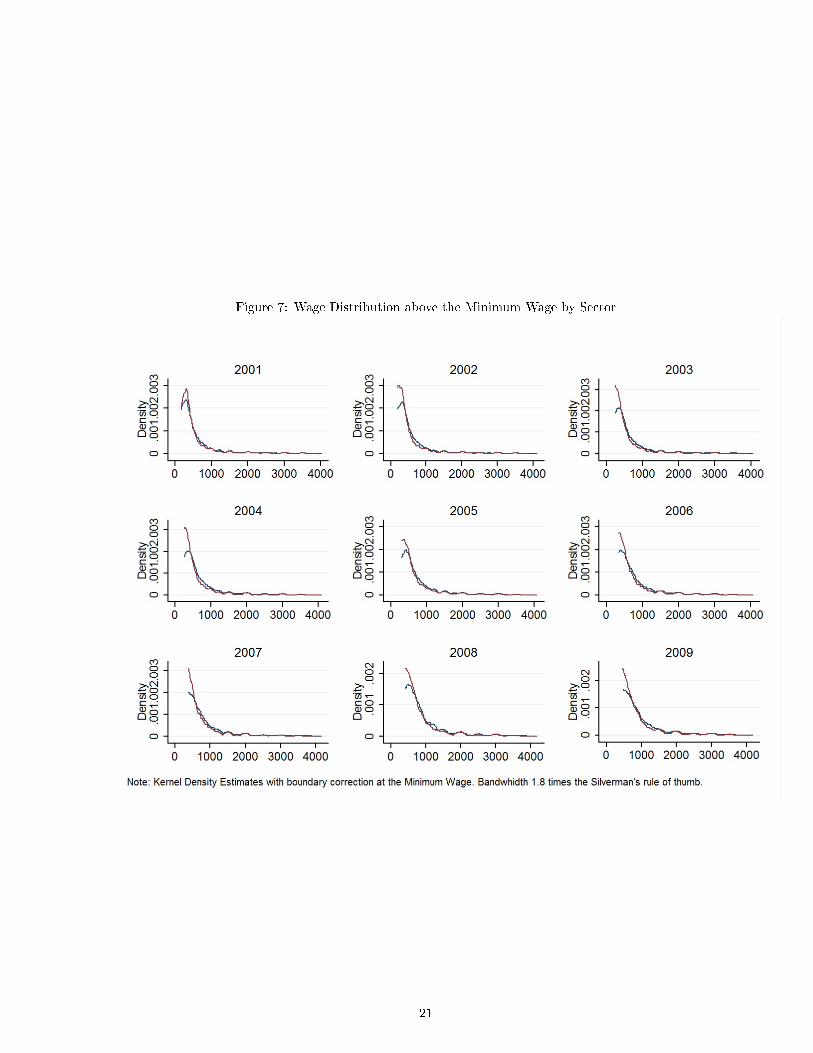
Figure 7: Wage Distribution above the Minimum Wage by Sector

21

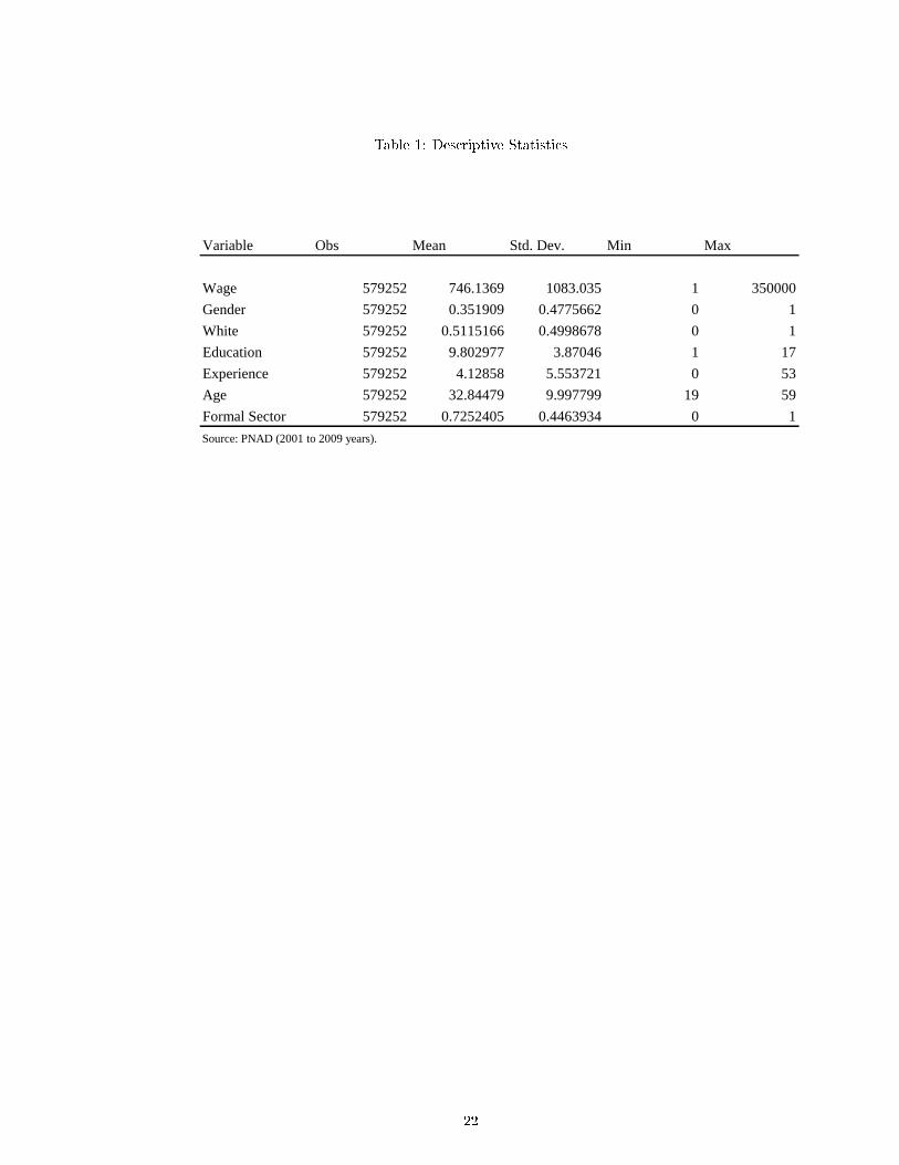
Table 1: Descriptive Statistics

Variable Obs Mean Std. Dev. Min Max

Wage 579252 746.1369 1083.035 1 350000

Gender 579252 0.351909 0.4775662 0 1

White 579252 0.5115166 0.4998678 0 1

Education 579252 9.802977 3.87046 1 17

Experience 579252 4.12858 5.553721 0 53

Age 579252 32.84479 9.997799 19 59

Formal Sector 579252 0.7252405 0.4463934 0 1

Source: PNAD (2001 to 2009 years).

22

Table 2: Descriptive Statistics by Sector

Formal Sector Informal Sector Difference

Wage 827.631*** 530.979*** 296.652***

(1.613) (2.694) (3.164)

Gender 0.358*** 0.336*** 0.022***

(0.001) (0.001) (0.001)

White 0.539*** 0.442*** 0.097***

(0.001) (0.001) (0.001)

Education 10.211*** 8.812*** 1.399***

(0.006) (0.010) (0.011)

Experience 4.525*** 3.133*** 1.392***

(0.009) (0.014) (0.016)

Age 33.256*** 31.851*** 1.405***

(0.015) (0.025) (0.029)

Minimum Wage Worker 0.1228632 0.163*** -0.040***

(0.001) (0.001) (0.001)

N 420,097 159,155 579,252

Source: PNAD (2001 to 2009). Heteroskedasticity Robust errors in parenthesis.

23

Table 3: Minimum and Subminimum Wage Conditional Probabilities

Pr(W=Mw) Pr(W<Mw)

Unconditional

0.1339 0.0798

Conditional on Gender

Male 0.1162 0.0719

Female 0.1667 0.0942

Conditional on Race

White 0.0942 0.0510

Nonwhite 0.1519 0.0897

Conditional on Education

Less than 5 years 0.1988 0.1849

Less than 12 years 0.1627 0.1155

More than 12 years 0.0527 0.0287

Conditional on Region

South 0.0577 0.0374

Southeast 0.0913 0.0438

Center-West 0.1233 0.0479

North 0.1874 0.1045

Northeast 0.2384 0.1692

Source: From 2001 to 2009 PNADs. N=579252.

24

Table 4: Model Parameters Estimates by Year

Coef/Se 2001 2002 2003 2004 2005 2006 2007 2008 2009

P1 0.202*** 0.217*** 0.206*** 0.232*** 0.180*** 0.157*** 0.113*** 0.192*** 0.121***

(0.006) (0.009) (0.005) (0.006) (0.006) (0.004) (0.003) (0.005) (0.003)

P2 0.256*** 0.356*** 0.289*** 0.293*** 0.349*** 0.262*** 0.176*** 0.304*** 0.208***

(0.007) (0.015) (0.007) (0.008) (0.011) (0.006) (0.004) (0.007) (0.005)

F(Mw) 0.253*** 0.260*** 0.311*** 0.291*** 0.328*** 0.400*** 0.446*** 0.345*** 0.434***

(0.005) (0.008) (0.004) (0.005) (0.007) (0.005) (0.005) (0.004) (0.005)

P1f

0.106*** 0.222*** 0.139*** 0.179*** 0.165*** 0.077*** -0.015*** 0.131*** 0.023***

(0.013) (0.021) (0.010) (0.012) (0.012) (0.007) (0.005) (0.008) (0.005)

P2f

0.191*** 0.231*** 0.223*** 0.226*** 0.258*** 0.213*** 0.152*** 0.264*** 0.186***

(0.006) (0.011) (0.006) (0.006) (0.009) (0.005) (0.003) (0.006) (0.004)

P1i

0.525*** 0.199*** 0.461*** 0.443*** 0.244*** 0.516*** 0.711*** 0.494*** 0.669***

(0.018) (0.038) (0.017) (0.019) (0.026) (0.013) (0.008) (0.016) (0.011)

P2i

0.475*** 0.801*** 0.539*** 0.557*** 0.756*** 0.484*** 0.289*** 0.506*** 0.331***

(0.018) (0.038) (0.017) (0.019) (0.026) (0.013) (0.008) (0.016) (0.011)

U 0.543*** 0.427*** 0.506*** 0.475*** 0.471*** 0.581*** 0.711*** 0.504*** 0.670***

(0.012) (0.024) (0.011) (0.013) (0.016) (0.010) (0.006) (0.010) (0.007)

r 0.772*** 0.781*** 0.792*** 0.798*** 0.816*** 0.819*** 0.823*** 0.832*** 0.847***

(0.002) (0.002) (0.002) (0.002) (0.002) (0.002) (0.002) (0.002) (0.002)

Sample Size: 71,397 71,051 68,319 68,196 65,755 62,587 58,269 58,241 55,502

Note: *** p<0.01, ** p<0.05, * p<0.1. Standard errors computed by 100 bootstrap replications.

25

Table 5: Distributional E�ects of the Minimum Wage

2001 2002 2003 2004 2005 2006 2007 2008 2009

E(lw)

Observed 5.994*** 6.054*** 6.152*** 6.220*** 6.322*** 6.400*** 6.489*** 6.578*** 6.658***

(0.004) (0.003) (0.004) (0.003) (0.003) (0.003) (0.003) (0.003) (0.003)

Latent 5.793*** 5.874*** 5.926*** 6.020*** 6.090*** 6.093*** 6.097*** 6.363*** 6.310***

(0.009) (0.014) (0.008) (0.009) (0.012) (0.010) (0.010) (0.008) (0.008)

Mw Effect 0.201*** 0.180*** 0.225*** 0.200*** 0.231*** 0.307*** 0.392*** 0.215*** 0.348***

(0.008) (0.012) (0.007) (0.008) (0.011) (0.009) (0.009) (0.007) (0.007)

Sd(Lw)

Observed 0.769*** 0.774*** 0.753*** 0.737*** 0.719*** 0.699*** 0.693*** 0.684*** 0.661***

(0.004) (0.004) (0.004) (0.004) (0.004) (0.003) (0.004) (0.003) (0.003)

Latent 0.916*** 0.929*** 0.916*** 0.885*** 0.901*** 0.881*** 0.897*** 0.846*** 0.851***

(0.006) (0.006) (0.006) (0.006) (0.007) (0.006) (0.009) (0.006) (0.006)

Mw Effect -0.147*** -0.155*** -0.163*** -0.149*** -0.182*** -0.182*** -0.204*** -0.162*** -0.190***

(0.004) (0.005) (0.003) (0.004) (0.005) (0.004) (0.006) (0.004) (0.004)

q 80 (lw)-q 20 (lw)

Observed 1.157*** 1.112*** 1.124*** 1.015*** 1.099*** 1.050*** 0.916*** 1.062*** 0.948***

(0.003) (0.020) (0.012) (0.016) (0.000) (0.000) (0.000) (0.000) (0.002)

Latent 1.419*** 1.476*** 1.267*** 1.386*** 1.386*** 1.386*** 1.447*** 1.204*** 1.204***

(0.022) (0.045) (0.019) (0.000) (0.012) (0.021) (0.015) (0.010) (0.012)

Mw Effect -0.262*** -0.364*** -0.143*** -0.372*** -0.288*** -0.336*** -0.531*** -0.142*** -0.256***

(0.022) (0.052) (0.022) (0.016) (0.012) (0.021) (0.015) (0.010) (0.012)

Gini

Observed 0.069*** 0.069*** 0.065*** 0.063*** 0.061*** 0.058*** 0.056*** 0.055*** 0.052***

(0.000) (0.000) (0.000) (0.000) (0.000) (0.000) (0.000) (0.000) (0.000)

Latent 0.087*** 0.087*** 0.085*** 0.081*** 0.081*** 0.080*** 0.080*** 0.072*** 0.074***

(0.001) (0.001) (0.001) (0.001) (0.001) (0.001) (0.001) (0.001) (0.000)

Mw Effect -0.018*** -0.018*** -0.019*** -0.017*** -0.021*** -0.022*** -0.024*** -0.017*** -0.022***

(0.001) (0.001) (0.000) (0.001) (0.001) (0.000) (0.000) (0.000) (0.000)

Sample Size: 71,397 71,051 68,319 68,196 65,755 62,587 58,269 58,241 55,502

Note: *** p<0.01, ** p<0.05, * p<0.1. Standard errors computed by 100 bootstrap replications.

26

Table 6: Role of Covariates: Estimates of the parameters by sub-groups

Parameters\Conditional On: Female Male Black White Educ<12 Educ>=12

P1 0.099*** 0.137*** 0.110*** 0.086*** 0.158*** 0.081***

(0.004) (0.004) (0.006) (0.003) (0.005) (0.003)

P2 0.174*** 0.231*** 0.201*** 0.166*** 0.227*** 0.184***

(0.007) (0.007) (0.012) (0.006) (0.006) (0.006)

F(Mw) 0.549*** 0.364*** 0.532*** 0.392*** 0.500*** 0.388***

(0.008) (0.006) (0.012) (0.006) (0.006) (0.006)

P1f

0.008 0.039*** -0.007 -0.017*** 0.015* 0.004

(0.007) (0.007) (0.013) (0.006) (0.009) (0.005)

P2f

0.155*** 0.205*** 0.190*** 0.144*** 0.213*** 0.160***

(0.006) (0.007) (0.011) (0.005) (0.006) (0.005)

P1i

0.699*** 0.638*** 0.737*** 0.705*** 0.721*** 0.641***

(0.017) (0.015) (0.026) (0.015) (0.011) (0.018)

P2i

0.301*** 0.362*** 0.263*** 0.295*** 0.279*** 0.359***

(0.017) (0.015) (0.026) (0.015) (0.011) (0.018)

U 0.726*** 0.632*** 0.689*** 0.749*** 0.615*** 0.735***

(0.010) (0.011) (0.016) (0.008) (0.011) (0.008)

r 0.868*** 0.837*** 0.843*** 0.858*** 0.798*** 0.879***

(0.003) (0.002) (0.007) (0.002) (0.003) (0.002)

Sample Size: 26,030 45,367 6,176 34,530 40,013 31,384

note: *** p<0.01, ** p<0.05, * p<0.1. Standard errors computed by a 100 bootstrap replications. Data from 2009 PNAD.

27

Table 7: Minimum Wage E�ects on Labor Tax Revenues

2001 2002 2003 2004 2005 2006 2007 2008 2009

R 0.977*** 0.966*** 0.954*** 0.959*** 0.929*** 0.904*** 0.866*** 0.903*** 0.863***

(0.004) (0.004) (0.004) (0.004) (0.004) (0.004) (0.004) (0.004) (0.008)

s/r 0.912*** 0.892*** 0.895*** 0.891*** 0.884*** 0.884*** 0.899*** 0.889*** 0.902***

(0.002) (0.002) (0.002) (0.002) (0.001) (0.002) (0.002) (0.002) (0.002)

Eh(w | s = 1)/Ef(w | s = 1) 1.241*** 1.219*** 1.265*** 1.249*** 1.243*** 1.334*** 1.410*** 1.229*** 1.348***

(0.008) (0.010) (0.007) (0.007) (0.010) (0.008) (0.010) (0.007) (0.015)

U.F(Mw) 0.137*** 0.111*** 0.157*** 0.138*** 0.154*** 0.233*** 0.317*** 0.174*** 0.291***

(0.006) (0.009) (0.006) (0.006) (0.008) (0.006) (0.006) (0.006) (0.006)

Sample Size: 71,397 71,051 68,319 68,196 65,755 62,587 58,269 58,241 55,502

Note: *** p<0.01, ** p<0.05, * p<0.1. Standard errors computed by 100 bootstrap replications.

28

Table 8: Formality vs. Wages - Linear Regression Estimates

Condit

ional

on

:

Yea

rC

oef

/Std

. E

rro

rN

Coef

/Std

. E

rror

NC

oef

/Std

. E

rror

NC

oef

/Std

. E

rro

rN

2001

0.0

22

***

55

49

80

.00

9***

47

15

70

.00

4***

36

47

70

.00

2***

25

34

2

(0.0

01

)(0

.00

1)

(0.0

01

)(0

.00

1)

2002

0.0

24

***

58

32

70

.00

7***

47

13

50

.00

2***

34

27

90

.00

02

35

21

(0.0

01

)(0

.00

1)

(0.0

01

)(0

.00

1)

2003

0.0

30

***

58

26

80

.01

0***

46

22

50

.00

4***

33

17

00

.00

3***

22

78

5

(0.0

01

)(0

.00

1)

(0.0

01

)(0

.00

1)

2004

0.0

24

***

62

58

60

.00

7***

50

12

70

.00

4***

36

89

70

.00

1*

23

10

5

(0.0

01

)(0

.00

1)

(0.0

01

)(0

.00

1)

2005

0.0

31

***

65

75

50

.00

5***

50

56

00

.00

1*

34

69

3-0

.00

12

12

76

(0.0

01

)(0

.00

1)

(0.0

01

)(0

.00

1)

2006

0.0

29

***

68

19

60

.00

6***

51

63

90

.00

1*

32

63

50

.00

01

99

97

(0.0

01

)(0

.00

1)

(0.0

01

)(0

.00

1)

2007

0.0

28

***

68

31

90

.00

6***

53

64

00

.00

1*

34

25

70

.00

02

15

43

(0.0

01

)(0

.00

1)

(0.0

01

)(0

.00

1)

2008

0.0

29

***

71

05

10

.00

5***

54

10

7-0

.00

03

40

91

-0.0

01

21

18

4

(0.0

01

)(0

.00

1)

(0.0

01

)(0

.00

1)

2009

0.0

12

***

71

39

70

.00

2***

54

91

8-0

.00

03

58

04

-0.0

01

*2

02

85

(0.0

01

)(0

.00

0)

(0.0

00

)(0

.00

0)

w>

0w

>M

ww

>1.5

Mw

w>

2M

w

Note

: *

** p

<0

.01

, ** p

<0

.05

, * p

<0

.1.

Coef

fici

ent

reff

ers

to t

he

elas

tici

ty o

f fo

rmal

ity w

ith

res

pec

t to

wag

es m

easu

red

at

the

min

imu

m w

age

bas

ed o

n a

lin

ear

pro

bab

ilit

y m

od

el.

29

Table 9: Descriptive Statistics by Sector: The role of Minimum Wage

Par

amet

ers\

Co

nd

itio

nal

On:

Fo

rmal

Sec

tor

Info

rmal

Sec

tor

Dif

fere

nce

Fo

rmal

Sec

tor

Info

rmal

Sec

tor

Dif

fere

nce

Wag

e8

27

.63

1***

53

0.9

79

***

29

6.6

52

***

90

0.6

93

***

76

0.9

00

***

13

9.7

93

***

(1.6

13

)(2

.69

4)

(3.1

64

)(1

.82

0)

(4.9

80

)(4

.42

9)

Gen

der

0.3

58

***

0.3

36

***

0.0

22

***

0.3

43

***

0.2

81

***

0.0

62

***

(0.0

01

)(0

.00

1)

(0.0

01

)(0

.00

1)

(0.0

02

)(0

.00

2)

Whit

e0

.53

9***

0.4

42

***

0.0

97

***

0.5

65

***

0.5

19

***

0.0

46

***

(0.0

01

)(0

.00

1)

(0.0

01

)(0

.00

1)

(0.0

02

)(0

.00

2)

Ed

uca

tio

n1

0.2

11

***

8.8

12

***

1.3

99

***

10

.38

6***

9.4

06

***

0.9

80

***

(0.0

06

)(0

.01

0)

(0.0

11

)(0

.00

6)

(0.0

14

)(0

.01

4)

Exp

erie

nce

4.5

25

***

3.1

33

***

1.3

92

***

4.7

30

***

3.6

06

***

1.1

23

***

(0.0

09

)(0

.01

4)

(0.0

16

)(0

.01

0)

(0.0

18

)(0

.02

1)

Age

33

.25

6***

31

.85

1***

1.4

05

***

33

.53

9***

33

.19

6***

0.3

42

***

(0.0

15

)(0

.02

5)

(0.0

29

)(0

.01

6)

(0.0

35

)(0

.03

7)

N4

20

,09

71

59

,15

55

79

,25

23

66

,06

58

9,3

97

45

5,4

62

W>

0W

>M

w

Sou

rce:

P

NA

D (

20

01

to 2

00

9).

Het

erosk

edas

tici

ty R

ob

ust

err

ors

in

par

enth

esis

.

30

Table 10: Placebo Tests: Discontinuity estimates using minimum wage values of other years

Yea

r2

00

12002

2003

2004

2005

2006

20

07

20

08

Co

ef/s

eC

oef

/se

Coef

/se

Coef

/se

Coef

/se

Coef

/se

Co

ef/s

eC

oef

/se

Mw

02

1.0

60

**

*

(0.0

63

)

Mw

03

0.1

73

**

*0.6

47***

(0.0

62

)(0

.06

8)

Mw

04

0.8

14

**

*0.4

90***

1.5

62***

(0.0

36

)(0

.17

1)

(0.0

81)

Mw

05

0.6

11

**

*0.5

46***

0.0

89***

1.1

00**

*

(0.0

16

)(0

.01

6)

(0.0

15)

(0.0

26)

Mw

06

0.7

24

**

*0.6

73***

0.5

24***

0.2

38**

*0

.585***

(0.0

14

)(0

.01

5)

(0.0

13)

(0.0

29)

(0.1

45)

Mw

07

1.0

66

**

*0.8

21***

0.6

01***

0.4

32**

*-0

.055

1.4

78***

(0.0

19

)(0

.01

4)

(0.0

21)

(0.0

18)

(0.2

04)

(0.0

84)

Mw

08

1.6

71

**

*1.5

78***

1.3

05***

1.2

33**

*1

.249***

1.2

80***

1.9

63

**

*

(0.0

33

)(0

.02

6)

(0.0

22)

(0.0

27)

(0.0

29)

(0.1

94)

(0.1

03

)

Mw

09

1.2

91

**

*1.2

83***

1.0

00***

0.8

68**

*1

.053***

0.6

58***

0.7

98

**

*1

.009

**

(0.0

24

)(0

.02

3)

(0.0

20)

(0.0

13)

(0.0

18)

(0.0

24)

(0.0

23

)(0

.48

9)

Ave

rage

0.9

26

0.8

62

0.8

47

0.7

74

0.7

08

1.1

39

1.3

80

1.0

09

Sam

ple

Siz

e:7

1,3

97

71,0

51

68,3

19

68,1

96

65,7

55

62,5

87

58

,26

95

8,2

41

Note

: *

** p

<0

.01

, ** p

<0

.05

, * p

<0

.1.

Sta

nd

ard

err

ors

com

pu

ted

by 1

00

boots

trap

rep

lica

tion

s.

31

Table 11: Robustness - Mccary's Density Discontinuity Estimator

Coef/Se 2001 2002 2003 2004 2005 2006 2007 2008 2009

P1 0.134*** 0.163*** 0.163*** 0.152*** 0.137*** 0.132*** 0.108*** 0.156*** 0.114***

(0.008) (0.004) (0.004) (0.005) (0.004) (0.003) (0.002) (0.007) (0.002)

P2 0.171*** 0.268*** 0.229*** 0.191*** 0.267*** 0.221*** 0.169*** 0.247*** 0.196***

(0.011) (0.007) (0.005) (0.007) (0.007) (0.004) (0.003) (0.010) (0.003)

F(Mw) 0.336*** 0.318*** 0.363*** 0.386*** 0.390*** 0.442*** 0.457*** 0.394*** 0.448***

(0.012) (0.005) (0.005) (0.007) (0.005) (0.004) (0.003) (0.009) (0.003)

P1f

-0.028* 0.098*** 0.056*** 0.030*** 0.073*** 0.031*** -0.023*** 0.068*** 0.011***

(0.017) (0.009) (0.008) (0.009) (0.008) (0.005) (0.004) (0.011) (0.004)

P2f

0.127*** 0.174*** 0.177*** 0.148*** 0.197*** 0.179*** 0.146*** 0.214*** 0.175***

(0.009) (0.005) (0.005) (0.005) (0.005) (0.004) (0.003) (0.009) (0.003)

P1i

0.683*** 0.397*** 0.573*** 0.635*** 0.424*** 0.592*** 0.723*** 0.590*** 0.688***

(0.021) (0.019) (0.014) (0.014) (0.018) (0.011) (0.007) (0.017) (0.009)

P2i

0.317*** 0.603*** 0.427*** 0.365*** 0.576*** 0.408*** 0.277*** 0.410*** 0.312***

(0.021) (0.019) (0.014) (0.014) (0.018) (0.011) (0.007) (0.017) (0.009)

U 0.695*** 0.568*** 0.608*** 0.657*** 0.596*** 0.647*** 0.723*** 0.598*** 0.689***

(0.019) (0.010) (0.008) (0.011) (0.010) (0.006) (0.004) (0.016) (0.005)

r 0.772*** 0.781*** 0.792*** 0.798*** 0.816*** 0.819*** 0.823*** 0.832*** 0.847***

(0.002) (0.002) (0.003) (0.002) (0.002) (0.002) (0.002) (0.002) (0.002)

Sample Size: 71,397 71,051 68,319 68,196 65,755 62,587 58,269 58,241 55,502

note: *** p<0.01, ** p<0.05, * p<0.1

32

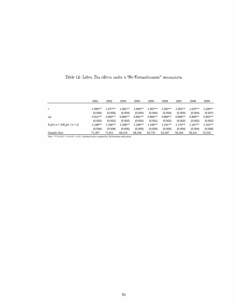
Table 12: Labor Tax e�ects under a �No Unemployment� assumption

2001 2002 2003 2004 2005 2006 2007 2008 2009

r 1.093*** 1.077*** 1.081*** 1.059*** 1.057*** 1.052*** 1.052*** 1.037*** 1.039***

(0.006) (0.005) (0.004) (0.004) (0.004) (0.004) (0.004) (0.004) (0.007)

s/r 0.912*** 0.892*** 0.895*** 0.891*** 0.884*** 0.884*** 0.899*** 0.889*** 0.902***

(0.002) (0.002) (0.002) (0.002) (0.001) (0.002) (0.002) (0.002) (0.002)

Eh(w | s = 1)/Eg(w | s = 1) 1.198*** 1.208*** 1.208*** 1.189*** 1.195*** 1.191*** 1.170*** 1.167*** 1.152***

(0.006) (0.006) (0.005) (0.005) (0.005) (0.005) (0.004) (0.004) (0.008)

Sample Size: 71,397 71,051 68,319 68,196 65,755 62,587 58,269 58,241 55,502

Note: *** p<0.01, ** p<0.05, * p<0.1. Standard errors computed by 100 bootstrap replications.

33

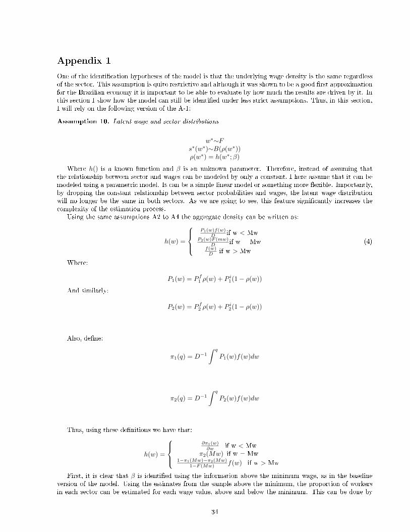
Appendix 1

One of the identi�cation hypotheses of the model is that the underlying wage density is the same regardlessof the sector. This assumption is quite restrictive and although it was shown to be a good �rst approximationfor the Brazilian economy it is important to be able to evaluate by how much the results are driven by it. Inthis section I show how the model can still be identi�ed under less strict assumptions. Thus, in this section,I will rely on the following version of the A-1:

Assumption 10. Latent wage and sector distributions

w∗∼Fs∗(w∗)∼B(ρ(w∗))ρ(w∗) = h(w∗;β)

Where h() is a known function and β is an unknown parameter. Therefore, instead of assuming thatthe relationship between sector and wages can be modeled by only a constant, I here assume that it can bemodeled using a parametric model. It can be a simple linear model or something more �exible. Importantly,by dropping the constant relationship between sector probabilities and wages, the latent wage distributionwill no longer be the same in both sectors. As we are going to see, this feature signi�cantly increases thecomplexity of the estimation process.

Using the same assumptions A2 to A4 the aggregate density can be written as:

h(w) =

P1(w)f(w)

D if w < MwP2(w)F (mw)

D if w = Mwf(w)D if w > Mw

(4)

Where:

P1(w) = P f1 ρ(w) + P i1(1− ρ(w))

And similarly:

P2(w) = P f2 ρ(w) + P i2(1− ρ(w))

Also, de�ne:

π1(q) = D−1∫ q

P1(w)f(w)dw

π2(q) = D−1∫ q

P2(w)f(w)dw

Thus, using these de�nitions we have that:

h(w) =

∂π1(w)∂w if w < Mw

π2(Mw) if w = Mw1−π1(Mw)−π2(Mw)

1−F (Mw) f(w) if w > Mw

First, it is clear that β is identi�ed using the information above the minimum wage, as in the baselineversion of the model. Using the estimates from the sample above the minimum, the proportion of workersin each sector can be estimated for each wage value, above and below the minimum. This can be done by

34

estimating a simple linear probability model, for example. In addition, using the same strategy to estimateP1 in the baseline model, P1(w) can be estimated by the density ratio above and below the minimum wage.Unfortunately, this alone does not allow us to recover the function P1(w) since it is necessary to recover atleast another point where P1(w) passes to recover the entire line. Things are worse regarding P2 and F(Mw).There is simply no simple algebra allowing us to recover the model parameters in the same way it was donefor the baseline model. There is no explicit solution for the model parameters that can be used to derive anestimator.

Thus, instead I will rely on the following fact:

MISE(θ) ≡∫

(h(w)− h(w|θ))2dw

MISE(θ∗) = 0

Where θ ≡ (P f1 , Pi1, P

f2 , P

i2, Uf , β) .This equation only means that, for the true values of the model

parameters, the di�erence between wage density that is implied by the parameters and the actual populationwage density is equal to zero.

MISE(θ) ≡ N−1N∑i=1

(h(wi)− h(wi|θ))2

Finally,

θ ≡ argminθ MISE(θ)

To reduce the dimension of the parameter vector, which can speed up the optimization, it is advisable to splitthe parameter vector into two parts. First, β and P1(Mw) are estimated. Then, there will actually only be

two free parameters with which to work: (P f1 , Pf2 ). All others are derived by the restrictions on probabilities

from assumption A2 and the estimate of P1(w).To implement the estimation of , the following algorithm can be used:1) Estimate β and P1(Mw).

2) Pick a vector ( Pf1 , Pf2 ).

3) Estimate the wage distribution given the value of θ implied by the choice of (P f1 , Pf2 ) , β and P1(Mw).

4) Calculate the value of MISE(θ). This can be done by comparing the wage density estimates based onobserved and simulated data.

5) Search over the set [0, 1]2. Select the set of parameters that minimize the empirical Mean IntegratedSquared Error.

A theoretical proof of consistency of this estimator is object of ongoing research.

35

Appendix 2 - Tax E�fects of minimum wage

To give an idea of the importance of the unemployment e�ects on the matter, I will also compute the e�ectsof minimum wages on tax based on a di�erent model. In this version, I will force the unemployment e�ects tobe equal to zero. By doing so, it is not possible to �nd a continuous latent wage distribution that generatesthe data. A discontinuous latent wage distribution can be nevertheless estimated. Formally, the model worksas follows. First, I will keep the �rst and third assumptions. The second assumption will be replaced by thefollowing:

Assumption 11. No Unemployment E�ects

Under the minimum wage a fraction P 1 of workers will earn the same wage as in the latent wage distri-bution. The remaining fraction will earn the minimum wage. These fractions can be sector-speci�c as in thebaseline model.

Notice that there is no Assumption 4 (continuity) in this case. Under these assumptions, the observedwage density will relate to the latent density by the following equation:

h(w) =

P1g(w) if w < Mw(1− P1)G(mw) if w = Mw

g(w) if w > Mw(5)

Where g(w) is the latent wage distribution based on this di�erent set of assumptions. In this case, weonly need to estimate P1. One way to do it is by recognizing that in this case:

P1 =Pr(w < Mw)

Pr(w < Mw) + Pr(w =Mw)

Therefore, a consistent estimator can be constructed by plugging in the maximum likelihood estimator ofthe respective quantities. With an estimate of P1 the latent wage density can be easily estimated by properlyreweighting the observed wage density. Next, the tax e�ects of minimum wages can be computed under the�No Unemployment� assumption. And it will be given by:

r ≡ t1

t0=s

ρ· Eh(w|s = 1)

Eg(w|s = 1)

Which is exactly the same expression without the unemployment component. Importantly, the expectedwages under the latent distribution also change, since the estimate of the latent distribution is di�erent underthis di�erent set of assumptions. To make this distinction clear, I denote the latent wage density under thismodel by g(w) and the distribution by G. Table 12 shows the estimates of r for the years of 2001 to 2009.Minimum wages have a su�ciently strong e�ect on average wages to compensate for the reduction in theformal sector share due to sector transition. This can be seen by positive MW e�ects on tax revenues basedon the no unemployment assumption.

36