EPA/600/R-05/061May 2005

Estimating and ProjectingImpervious Cover in the

Southeastern United States

by

Linda R. ExumSandra L. Bird

James Harrison1

Christine A. Perkins2

published by

Ecosystems Research DivisionNational Exposure Research LaboratoryU.S. Environmental Protection Agency

Athens, GA 30605-2700

1 U.S. Environmental Protection Agency Region 4

Atlanta, Georgia

2 Computer Sciences CorporationAthens, Georgia 30605-2700

U.S. Environmental Protection AgencyOffice of Research and Development

Washington, DC 20460

Notice

The research described in this document was funded by the U.S. Environmental Protection Agency through the Office of Research and Development and was conducted at the Ecosystems Research Division of the U.S. Environmental Protection Agency, National Exposure Research Laboratory in Athens, Georgia. Mention of trade names or commercial products does not constitute endorsement or recommendation for use.

ii

Acknow ledgments

We wish to thank Lourdes Prieto for her immense help in lending GIS technical assistance, including helping determine impervious cover during the test data set development. We also thank Stephen Alberty for his development of the GIS Cover Tool and helping determine impervious cover during the test data set development.

Foreword

Complete identification and eventual prevention of urban water quality problems pose significant monitoring, “smart growth” and water quality management challenges. Uncontrolled increase of impervious surface areas (roads, buildings and parking lots) causes detrimental hydrologic changes, stream channel erosion, habitat degradation and severe impairment of aquatic communities. In conjunction with the U.S. Environmental Protection Agency, Region 4­Atlanta, we provide a multiple data source estimation of imperviousness in the southeastern U.S. These estimates demonstrate an inexpensive method of determining impervious cover with known accuracy at the watershed and sub-watershed scales plus characterization of the change in imperviousness over time. In addition, this report estimates future impervious cover in the southeastern U.S. using the multiple data source technique. These estimates can guide in-situ monitoring to confirm problems, aid listing of impaired waters under Section 303(d) of the Clean Water Act and total maximum daily load (TMDL) development, provide reliable scientific information to energize sound local planning and land-use decisions, and promote protection and restoration of urban streams.

Rosemarie C. Russo, Ph.D. Director Ecosystems Research Division Athens, Georgia

"When we see land as a community to which we belong, we may begin to use it with love and respect." --Aldo Leopold

iii

Abstract

Urban/suburban land use is the most rapidly growing land use class. Along with increased development inevitably comes increased impervious surface--areas preventing infiltration of water into the underlying soil. The extensive hydrological alteration of watersheds associated with increased impervious cover is very difficult to control and correct relative to the impact of urbanization on waterways. Development practices that reduce impervious area and include preventative strategies to protect water quality are more effective and less costly than remedial restoration efforts. Simple and reliable methods to estimate and project impervious cover can help identify areas where a watershed is at risk of changing rapidly from a system with relatively pristine streams to one with significant symptoms of degradation. In this study, a method for estimating and projecting impervious cover for 12 and 14 digit HUCs over a large area was developed and tested. These methods were then applied in EPA Region 4’s eightsoutheastern states to provide the Region with a screening tool to guide monitoring and educational efforts.

iv

Table of C ontents

Abstract . . . . . . . . . . . . . . . . . . . . . . . . . . . . . . . . . . . . . . . . . . . . . . . . . . . . . . . . . . . . . . . . . . . . . . . . . . . . . . . . . . . iv

1. Background and Introduction . . . . . . . . . . . . . . . . . . . . . . . . . . . . . . . . . . . . . . . . . . . . . . . . . . . . . . . . . . . . . . . . 11.1 Stream Biotic Response to Impervious Cover . . . . . . . . . . . . . . . . . . . . . . . . . . . . . . . . . . . . . . . . . . . . 31.2 Using Impervious Cover as a Regional Indicator . . . . . . . . . . . . . . . . . . . . . . . . . . . . . . . . . . . . . . . . . 51.3 Study Objectives . . . . . . . . . . . . . . . . . . . . . . . . . . . . . . . . . . . . . . . . . . . . . . . . . . . . . . . . . . . . . . . . . . 8

2. Test Data Set Development . . . . . . . . . . . . . . . . . . . . . . . . . . . . . . . . . . . . . . . . . . . . . . . . . . . . . . . . . . . . . . . . . 102.1 Digital Orthophoto Quarter Quadrangles (DO QQs) . . . . . . . . . . . . . . . . . . . . . . . . . . . . . . . . . . . . . . 102.2 Data Collection System . . . . . . . . . . . . . . . . . . . . . . . . . . . . . . . . . . . . . . . . . . . . . . . . . . . . . . . . . . . . 122.3 Sampling System Design . . . . . . . . . . . . . . . . . . . . . . . . . . . . . . . . . . . . . . . . . . . . . . . . . . . . . . . . . . . 142.4 Sample Size . . . . . . . . . . . . . . . . . . . . . . . . . . . . . . . . . . . . . . . . . . . . . . . . . . . . . . . . . . . . . . . . . . . . . 152.5 Analyst Variability . . . . . . . . . . . . . . . . . . . . . . . . . . . . . . . . . . . . . . . . . . . . . . . . . . . . . . . . . . . . . . . 162.6 Final Sampling Scheme . . . . . . . . . . . . . . . . . . . . . . . . . . . . . . . . . . . . . . . . . . . . . . . . . . . . . . . . . . . . 182.7 Results . . . . . . . . . . . . . . . . . . . . . . . . . . . . . . . . . . . . . . . . . . . . . . . . . . . . . . . . . . . . . . . . . . . . . . . . . 18

3. Development of a Multiple Data Source Method for Regional Scale Estimates of Impervious Cover . . . . . . . . 263.1 Population Density Relationships . . . . . . . . . . . . . . . . . . . . . . . . . . . . . . . . . . . . . . . . . . . . . . . . . . . . 263.2 Use of Categorized Satellite Imagery . . . . . . . . . . . . . . . . . . . . . . . . . . . . . . . . . . . . . . . . . . . . . . . . . 273.3 Multiple Data Source Approach . . . . . . . . . . . . . . . . . . . . . . . . . . . . . . . . . . . . . . . . . . . . . . . . . . . . . 343.4 Comparison of NLCD only and Multiple Data Source (MDS) Approach . . . . . . . . . . . . . . . . . . . . . 37

4. Impervious Cover in the Southeastern United States . . . . . . . . . . . . . . . . . . . . . . . . . . . . . . . . . . . . . . . . . . . . . 424.1 Alabama . . . . . . . . . . . . . . . . . . . . . . . . . . . . . . . . . . . . . . . . . . . . . . . . . . . . . . . . . . . . . . . . . . . . . . . 454.2 Florida . . . . . . . . . . . . . . . . . . . . . . . . . . . . . . . . . . . . . . . . . . . . . . . . . . . . . . . . . . . . . . . . . . . . . . . . . 474.3 Georgia . . . . . . . . . . . . . . . . . . . . . . . . . . . . . . . . . . . . . . . . . . . . . . . . . . . . . . . . . . . . . . . . . . . . . . . . 494.4 Kentucky . . . . . . . . . . . . . . . . . . . . . . . . . . . . . . . . . . . . . . . . . . . . . . . . . . . . . . . . . . . . . . . . . . . . . . . 514.5 Mississippi . . . . . . . . . . . . . . . . . . . . . . . . . . . . . . . . . . . . . . . . . . . . . . . . . . . . . . . . . . . . . . . . . . . . . 534.6 North Carolina . . . . . . . . . . . . . . . . . . . . . . . . . . . . . . . . . . . . . . . . . . . . . . . . . . . . . . . . . . . . . . . . . . 554.7 South Carolina . . . . . . . . . . . . . . . . . . . . . . . . . . . . . . . . . . . . . . . . . . . . . . . . . . . . . . . . . . . . . . . . . . 574.8 Tennessee . . . . . . . . . . . . . . . . . . . . . . . . . . . . . . . . . . . . . . . . . . . . . . . . . . . . . . . . . . . . . . . . . . . . . . 59

5. Future Impervious Cover Projections for the Southeastern United States . . . . . . . . . . . . . . . . . . . . . . . . . . . . . . 615.1 The Nature of Errors in Population Projections . . . . . . . . . . . . . . . . . . . . . . . . . . . . . . . . . . . . . . . . . 615.2 Impervious Cover Projection Method . . . . . . . . . . . . . . . . . . . . . . . . . . . . . . . . . . . . . . . . . . . . . . . . . 63

5.2.1 Residential Component . . . . . . . . . . . . . . . . . . . . . . . . . . . . . . . . . . . . . . . . . . . . . . . . . . . . 635.2.2 Commercial/Industrial Component . . . . . . . . . . . . . . . . . . . . . . . . . . . . . . . . . . . . . . . . . . . 655.2.3 Major Highway Component . . . . . . . . . . . . . . . . . . . . . . . . . . . . . . . . . . . . . . . . . . . . . . . . 67

5.3 Impervious Cover Pro jections . . . . . . . . . . . . . . . . . . . . . . . . . . . . . . . . . . . . . . . . . . . . . . . . . . . . . . . 675.3.1 Alabama . . . . . . . . . . . . . . . . . . . . . . . . . . . . . . . . . . . . . . . . . . . . . . . . . . . . . . . . . . . . . . . 695.3.2 Florida . . . . . . . . . . . . . . . . . . . . . . . . . . . . . . . . . . . . . . . . . . . . . . . . . . . . . . . . . . . . . . . . 735.3.3 Georgia . . . . . . . . . . . . . . . . . . . . . . . . . . . . . . . . . . . . . . . . . . . . . . . . . . . . . . . . . . . . . . . . 775.3.4 Kentucky . . . . . . . . . . . . . . . . . . . . . . . . . . . . . . . . . . . . . . . . . . . . . . . . . . . . . . . . . . . . . . . 815.3.5 Mississippi . . . . . . . . . . . . . . . . . . . . . . . . . . . . . . . . . . . . . . . . . . . . . . . . . . . . . . . . . . . . . 855.3.6 North Carolina . . . . . . . . . . . . . . . . . . . . . . . . . . . . . . . . . . . . . . . . . . . . . . . . . . . . . . . . . . 895.3.7 South Carolina . . . . . . . . . . . . . . . . . . . . . . . . . . . . . . . . . . . . . . . . . . . . . . . . . . . . . . . . . . 935.3.8 Tennessee . . . . . . . . . . . . . . . . . . . . . . . . . . . . . . . . . . . . . . . . . . . . . . . . . . . . . . . . . . . . . . 97

5.4 Using the Impervious Cover Projections . . . . . . . . . . . . . . . . . . . . . . . . . . . . . . . . . . . . . . . . . . . . . . 101

6. Conclusions and Recommendations . . . . . . . . . . . . . . . . . . . . . . . . . . . . . . . . . . . . . . . . . . . . . . . . . . . . . . . . . 102

References . . . . . . . . . . . . . . . . . . . . . . . . . . . . . . . . . . . . . . . . . . . . . . . . . . . . . . . . . . . . . . . . . . . . . . . . . . . . . . . 104

Appendix . . . . . . . . . . . . . . . . . . . . . . . . . . . . . . . . . . . . . . . . . . . . . . . . . . . . . . . . . . . . . . . . . . . . . . . . . . . . . . . . 113

v

List of Figures

Figure 1.1 Multiple Data Source Impervious Area for North Carolina Piedmont Benthic Site Watersheds . . . . . . 6Figure 1.2 Percent Degraded Piedmont Sites vs. Total Impervious Area . . . . . . . . . . . . . . . . . . . . . . . . . . . . . . . . . 7Figure 2.1 Examples of Features in DOQQ scenes. . . . . . . . . . . . . . . . . . . . . . . . . . . . . . . . . . . . . . . . . . . . . . . . . 12Figure 2.2 Captured Screen from the Cover Tool Extension Software . . . . . . . . . . . . . . . . . . . . . . . . . . . . . . . . . 14Figure 2.3 Example of Difference (Unassigned Points) Between Analyst 1 and Analyst 2. . . . . . . . . . . . . . . . . . 15Figure 2.4 Sample Size and Deviation vs. Grid Spacing. . . . . . . . . . . . . . . . . . . . . . . . . . . . . . . . . . . . . . . . . . . . . 16Figure 2.5 Comparison of Impervious Cover by Analyst. . . . . . . . . . . . . . . . . . . . . . . . . . . . . . . . . . . . . . . . . . . . 17Figure 2.6 Impervious Cover Results from the DOQQ Interpretation for Frederick County, MD . . . . . . . . . . . . . 20Figure 2.7 Impervious Cover Results from the DOQQ Interpretation of 13 Atlanta Area HUCs . . . . . . . . . . . . . 24Figure 3.1 The three relationships between population density and %TIA . . . . . . . . . . . . . . . . . . . . . . . . . . . . . . 28Figure 3.2 Land cover map of the eight Southeastern states using the NLCD92 . . . . . . . . . . . . . . . . . . . . . . . . . . 30Figure 3.3 Total acreage categorized as residential (combined high and low density) in the NLCD92 data . . . . . 31Figure 3.4 Impervious cover for Frederick County, MD watersheds measured from aerial photographs vs that

estimated from categorized satellite imagery . . . . . . . . . . . . . . . . . . . . . . . . . . . . . . . . . . . . . . . . . . . . 32Figure 3.5 Impervious cover for 13 Atlanta, GA area HUCs measured from aerial photographs vs that estimated

from categorized satellite imagery . . . . . . . . . . . . . . . . . . . . . . . . . . . . . . . . . . . . . . . . . . . . . . . . . . . . 34Figure 3.6 Impervious cover for Frederick County, MD watersheds measured from aerial photographs vs that

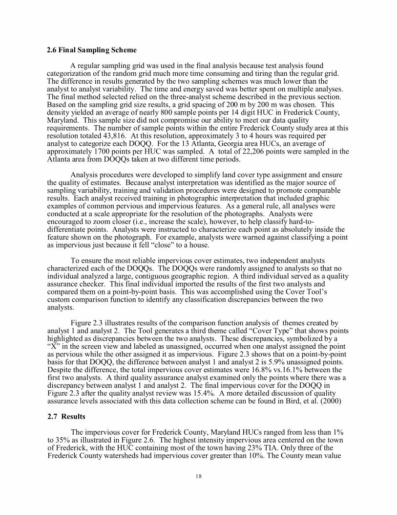
estimated from Multiple Data Sources . . . . . . . . . . . . . . . . . . . . . . . . . . . . . . . . . . . . . . . . . . . . . . . . . 36Figure 3.7 Impervious cover for 13 Atlanta area HUCs measured from aerial photographs vs that estimated from

Multiple Data Sources . . . . . . . . . . . . . . . . . . . . . . . . . . . . . . . . . . . . . . . . . . . . . . . . . . . . . . . . . . . . . 37Figure 3.8 Estimated 1993 %TIA for 1624 Georgia 12 digit HUCs . . . . . . . . . . . . . . . . . . . . . . . . . . . . . . . . . . . 40Figure 3.9 Estimated 1999 %TIA for 1624 Georgia 12 digit HUCs . . . . . . . . . . . . . . . . . . . . . . . . . . . . . . . . . . . 41Figure 4.1 Southeastern United States impervious cover for 2000 . . . . . . . . . . . . . . . . . . . . . . . . . . . . . . . . . . . . 44Figure 4.2 Alabama impervious cover for 2000 . . . . . . . . . . . . . . . . . . . . . . . . . . . . . . . . . . . . . . . . . . . . . . . . . . . 46Figure 4.3 Florida impervious cover for 2000 . . . . . . . . . . . . . . . . . . . . . . . . . . . . . . . . . . . . . . . . . . . . . . . . . . . . 48Figure 4.4 Georgia impervious cover for 2000 . . . . . . . . . . . . . . . . . . . . . . . . . . . . . . . . . . . . . . . . . . . . . . . . . . . 50Figure 4.5 Kentucky impervious cover for 2000 . . . . . . . . . . . . . . . . . . . . . . . . . . . . . . . . . . . . . . . . . . . . . . . . . . 52Figure 4.6 Mississippi impervious cover for 2000 . . . . . . . . . . . . . . . . . . . . . . . . . . . . . . . . . . . . . . . . . . . . . . . . . 54Figure 4.7 North Carolina impervious cover for 2000 . . . . . . . . . . . . . . . . . . . . . . . . . . . . . . . . . . . . . . . . . . . . . . 56Figure 4.8 South Carolina impervious cover for 2000 . . . . . . . . . . . . . . . . . . . . . . . . . . . . . . . . . . . . . . . . . . . . . . 58Figure 4.9 Tennessee impervious cover for 2000 . . . . . . . . . . . . . . . . . . . . . . . . . . . . . . . . . . . . . . . . . . . . . . . . . . 60Figure 5.1 High Intensity Commercial/Industrial area (meters) vs. population for North Carolina . . . . . . . . . . . 66Figure 5.2 Alabama projected impervious cover out to 2025. . . . . . . . . . . . . . . . . . . . . . . . . . . . . . . . . . . . . . . . . 70Figure 5.3 Alabama Projected %TIA as % of Area out to 2025 . . . . . . . . . . . . . . . . . . . . . . . . . . . . . . . . . . . . . . 71Figure 5.4 Total River Miles in Alabama by %TIA Category out to 2025 . . . . . . . . . . . . . . . . . . . . . . . . . . . . . . 72Figure 5.5 Florida projected impervious cover out to 2025. . . . . . . . . . . . . . . . . . . . . . . . . . . . . . . . . . . . . . . . . . 74Figure 5.6 Florida Projected %TIA as % of Area out to 2025 . . . . . . . . . . . . . . . . . . . . . . . . . . . . . . . . . . . . . . . . 75Figure 5.7 Total River Miles in Florida by %TIA Category out to 2025 . . . . . . . . . . . . . . . . . . . . . . . . . . . . . . . . 76Figure 5.8 Georgia impervious cover out to 2010. . . . . . . . . . . . . . . . . . . . . . . . . . . . . . . . . . . . . . . . . . . . . . . . . 78Figure 5.9 Georgia Projected %TIA as % of Area out to 2010 . . . . . . . . . . . . . . . . . . . . . . . . . . . . . . . . . . . . . . . 79Figure 5.10 Total River Miles in Georgia by %TIA Category out to 2010 . . . . . . . . . . . . . . . . . . . . . . . . . . . . . . . 80Figure 5.11 Kentucky impervious cover out to 2030. . . . . . . . . . . . . . . . . . . . . . . . . . . . . . . . . . . . . . . . . . . . . . . . 82Figure 5.12 Kentucky Projected %TIA as % of Area out to 2030 . . . . . . . . . . . . . . . . . . . . . . . . . . . . . . . . . . . . . . 83Figure 5.13 Total River Miles in Kentucky by %TIA Category out to 2030 . . . . . . . . . . . . . . . . . . . . . . . . . . . . . . 84Figure 5.14 Mississippi impervious cover out to 2015. . . . . . . . . . . . . . . . . . . . . . . . . . . . . . . . . . . . . . . . . . . . . . . 86Figure 5.15 Mississippi Projected %TIA as % of Area out to 2015 . . . . . . . . . . . . . . . . . . . . . . . . . . . . . . . . . . . . 87Figure 5.16 Total River Miles in Mississippi by %TIA Category out to 2015 . . . . . . . . . . . . . . . . . . . . . . . . . . . . 88Figure 5.17 North Carolina impervious cover out to 2030. . . . . . . . . . . . . . . . . . . . . . . . . . . . . . . . . . . . . . . . . . . . 90Figure 5.18 North Carolina Projected %TIA as % of Area out to 2030 . . . . . . . . . . . . . . . . . . . . . . . . . . . . . . . . . 91Figure 5.19 Total River Miles in North Carolina by %TIA Category out to 2030 . . . . . . . . . . . . . . . . . . . . . . . . . 92Figure 5.20 South Carolina impervious cover out to 2025 . . . . . . . . . . . . . . . . . . . . . . . . . . . . . . . . . . . . . . . . . . . 94Figure 5.21 South Carolina Projected %TIA as % of Area out to 2025 . . . . . . . . . . . . . . . . . . . . . . . . . . . . . . . . . 95Figure 5.22 Total River Miles in South Carolina by %TIA Category out to 2025 . . . . . . . . . . . . . . . . . . . . . . . . . 96Figure 5.23 Tennessee impervious cover out to 2020 . . . . . . . . . . . . . . . . . . . . . . . . . . . . . . . . . . . . . . . . . . . . . . . 98Figure 5.24 Tennessee Projected %TIA as % of Area out to 2020 . . . . . . . . . . . . . . . . . . . . . . . . . . . . . . . . . . . . . 99Figure 5.25 Total River Miles in Tennessee by %TIA Category out to 2020 . . . . . . . . . . . . . . . . . . . . . . . . . . . . 100

vi

List of Tables

Table 2.1 Impervious Cover Interpretation of 1989 HUCs for Frederick County, Maryland . . . . . . . . . . . . . . . . 21Table 2.2 Impervious Cover Interpretation of 1993 (Black & White) DOQQs and 1999 (Color) DOQQs of 13 12

digit HUCs in the Atlanta, Georgia Area . . . . . . . . . . . . . . . . . . . . . . . . . . . . . . . . . . . . . . . . . . . . . . . 25Table 3.1 Empirical relationships between population density and impervious area . . . . . . . . . . . . . . . . . . . . . . 27Table 3.2 Impervious Cover for Frederick County, Maryland NLCD92 Land Cover Categories . . . . . . . . . . . . 33Table 3.3 Percent Total Impervious Area (%TIA) Results for North Georgia Watersheds . . . . . . . . . . . . . . . . . 38Table 3.4 Evaluation of Impervious Cover Status of Georgia Watersheds/HUC’s . . . . . . . . . . . . . . . . . . . . . . . . 39Table 4.1 %TIA as a Percentage of the Total Land Area of Each Southeastern State Using the 2000

Census and the Multiple Data Source Approach . . . . . . . . . . . . . . . . . . . . . . . . . . . . . . . . . . . . . . . . . 43Table 5.1 Sources and Dates of Population Projections for Each Southeastern State . . . . . . . . . . . . . . . . . . . . . 64Table 5.2 2000 U.S. Census and State Population Projections for the Southeastern United States . . . . . . . . . . . 68Table 5.3 %TIA as a Percentage of the Total Land Area of Alabama out to 2025 . . . . . . . . . . . . . . . . . . . . . . . . 71Table 5.4 Total River Miles in Alabama by %TIA category out to 2025 . . . . . . . . . . . . . . . . . . . . . . . . . . . . . . . 72Table 5.5 %TIA as a Percentage of the Total Land Area of Florida out to 2025 . . . . . . . . . . . . . . . . . . . . . . . . . 75Table 5.6 Total River Miles in Florida per TIA category out to 2025 . . . . . . . . . . . . . . . . . . . . . . . . . . . . . . . . . 76Table 5.7 %T IA as a Percentage of the Total Land Area of Georgia . . . . . . . . . . . . . . . . . . . . . . . . . . . . . . . . . . 79Table 5.8 Total River Miles in Georgia per TIA category . . . . . . . . . . . . . . . . . . . . . . . . . . . . . . . . . . . . . . . . . . 80Table 5.9 %TIA as a Percentage of the Total Land Area of Kentucky out to 2030 . . . . . . . . . . . . . . . . . . . . . . . 83Table 5.10 Total River Miles in Kentucky per TIA category out to 2030 . . . . . . . . . . . . . . . . . . . . . . . . . . . . . . . 84Table 5.11 %TIA as a Percentage of the Total Land Area of Mississippi out to 2015 . . . . . . . . . . . . . . . . . . . . . . 87Table 5.12 Total River Miles in Mississippi per TIA category . . . . . . . . . . . . . . . . . . . . . . . . . . . . . . . . . . . . . . . 88Table 5.13 %TIA as a Percentage of the Total Land Area of North Carolina out to 2030 . . . . . . . . . . . . . . . . . . . 91Table 5.14 Total River Miles in North Carolina per TIA category out to 2030 . . . . . . . . . . . . . . . . . . . . . . . . . . . 92Table 5.15 %TIA as a Percentage of the Total Land Area of South Carolina . . . . . . . . . . . . . . . . . . . . . . . . . . . . 95Table 5.16 Total River Miles in South Carolina per TIA category . . . . . . . . . . . . . . . . . . . . . . . . . . . . . . . . . . . . . 96Table 5.17 %TIA as a Percentage of the Total Land Area of Tennessee out to 2020 . . . . . . . . . . . . . . . . . . . . . . 99Table 5.18 Total River Miles in Tennessee per TIA category . . . . . . . . . . . . . . . . . . . . . . . . . . . . . . . . . . . . . . . 100

vii

1. Background and Introduction

Nonpoint source pollution (NPS), i.e., pollution from diffuse sources such asurban/suburban areas and farmlands, is now recognized as the primary threat to water quality in the United States (U.S. Environmental Protection Agency 1994). The pressure on waterresources due to urbanization is rapidly increasing as the U.S. population grows. Urban area in the contiguous United States increased 26% and roads increased 2% from 1982 to 1992, while rangeland and cropland/pasture each reduced 2%, respectively (USDA 1997). Between 1992 and 1997 the estimated urban area in the contiguous United States increased another 6 million acres, or 11%, while grassland pasture and rangeland decreased by 11 million acres or another 2% (USDA 2003). In 1997 USDA identified a new subcategory named “rural residential” as part of its miscellaneous uses, a category that includes marshes, swamps, bare rock areas, deserts and transitional areas (USDA 2003). Miscellaneous uses also increased significantly between 1992 and 1997, due in large part to the increase of rural residential.

The U.S. population more than doubled from 133 million to 281 million people between1945 and 2000, with the total households increasing to 106 million, a quarter of which consistedof a single individual. Besides more land being converted to residential uses, especially for homes, new residential areas also require land for schools, office buildings, shopping sites, andother supporting commercial and industrial uses. The amount of urban land in the U.S. has risen steadily from 15 million acres in 1945 to an estimated 66 million acres in 1997, converted mostly from pasture, range and forest land (USDA 2003).

The pace of urban growth in the Southeastern United States is unprecedented. A recent National Geographic map (Mitchell and Leen 2001) illustrates this extremely rapid urban/suburban expansion using Department of Defense “city lights” data from two time periods, 1993 and the “present.” Huge areas of “sprawl” growth are particularly evident throughout the Southeast and are most heavily concentrated in the area between Atlanta, GA and Raleigh, NC. Based on National Resources Inventory data, developed land increased between 1992 and 1997 in the Southeast as follows: Alabama (16.2%); Florida (18.9%); Georgia (27.4%); Kentucky (12.8%); Mississippi (16.2%); North Carolina (15.1%); South Carolina(20.8%); and Tennessee (20.4%) (USDA 2000). A probability sample of landscape trends for ecoregions of the mid-Atlantic and Southeastern United States documented an increase in urban area for the Southern Piedmont from 12% to over 16% between 1972 and 2000, the most rapid urban growth among the ecoregions sampled (Griffith, et al. 2003).

Rapid growth is expected to continue. Preliminary forecasts expect urban land in the study area of the Southern Forest Resource Assessment to increase from 20 million acres in 1992 to 55 million acres in 2020, and to 81 million acres in 2040 (Wear and Greis, 2002). This urban expansion will likely come at the expense of both agricultural and forest areas. Regions in the Southeast likely to be most affected by future growth are the Piedmont, the Lower Atlantic and Gulf Coastal Plains and the Southern Appalachians.

Fundamental social and economic forces govern conversion of land from uses of less value to uses of greater value. Production of wealth drives much economic activity and growth. In the Willamette River Basin (Oregon, USA), the dollar value of developed land relative to its dollar value for dry land (non-irrigated) agriculture was 59 times for land prepared for homes, 253 times for land with single family homes, up to 552 times for land in commercial use, and390 to 2535 times for industrial use (Hulse and Ribe 2000). This tremendous increase in landvaluation places intense economic pressure promoting development of land to urban use whenever the demand exists.

1

Urban growth produces many stresses on water quality. Often sanitary sewer infrastructure is not properly maintained and capacity is insufficient. Combined and sanitarysewer overflow, leaking sewer pipes and faulty septic systems lead to effluent inadvertently reaching waterways. Sedimentation from construction activities, inadequate control of pointsources, polluted runoff and illicit discharges lead to a decline in water quality (Harrison, et al. 2001).

Arguably, the most difficult to control and correct relative to the impact of urbanizationon water courses is the extensive hydrologic alteration of watersheds , i.e., excessive (as well as polluted) runoff from impervious surfaces and riparian area degradation. Along with increaseddevelopment inevitably comes increased impervious surface--areas preventing infiltration of water into the underlying soil. Roadways, parking lots and rooftops account for the majority of impervious area. It is estimated that there are more than 105,200,000 parking spaces in the U.S., with a ratio of off-street spaces to on-street spaces roughly two-to-one (NCDENR 2002). Studies in some metropolitan areas indicate that there are seven times more parking spaces than there are vehicles.

In addition to extremely deleterious ecological and water quality impacts, flooding is also a devastating result of the urban hydrologic alteration (Inman 2000; Inman 1995), a stress that is only sporadically regulated at the local level. Hydrologic (Poff, et al. 1997; Richter, et al. 1996) and physical stresses (Gaff 2001), as well as chemical contamination, must be addressed to protect and restore urban water resources.

Increased imperviousness causes a well-known cascade of damaging results to streams (Wolman 1967 and Caraco , et al. 1998). Detrimental hydrologic changes cause more frequent, higher peak flows (Jennings and Jarnagin, 2002) and lower water tables and base flows which can influence both riparian (Groffman, et al. 2003) and aquatic communities. Due to lowered base flows, streams have reduced resilience to recover from drought conditions. Watershed runoff can increase by two to over five times normal for forested catchments as impervious area increases from the 10 to 20% range to 75 to100% respectively (Arnold and Gibbons 1996). Altered high flow regimes also increase stream bank erosion and channel enlargement producing significant sedimentation from the stream channel itself. The few available quantitative studies of channel changes due to urbanization indicate that from one-half (1/2) to three-quarters (3/4) of stream sediment load originates from channel erosion (Trimble 1997; Dartiguenave andMaidment 1997; Corbett, et al. 1997) rather than upland sources. The resulting unstable channel often evidences highly degraded aquatic habitat, largely due to unstable substrates. The end result of these stresses is usually severe biological impairment and poor aquatic community integrity. (See both Paul and Meyer 2001, and Center for Watershed Protection 2003 for comprehensive reviews of impacts of impervious area on aquatic systems.)

Often, other ecological stresses compound hydrologic impacts from imperviousness. Summer stream temperatures can be elevated due to runoff from pavement and structures, placing additional stress on the biological communities. Riparian alterations regularly exacerbate stream channel erosion and increase stream temperatures further. Additional habitat degradation often ensues from reduced input of large woody debris (LWD), and from increased stream crossings by roads, sewers and other structures that create barriers to fish movement (Paul and Meyer 2001). Impervious surfaces channel pollutants directly into waterways, preventing processing of these pollutants in soils. Higher pollutant loads, particularly oils, otherpetroleum products and metals are typically associated with roadways, while biocides (pesticides and herbicides) are generally associated with managed landscapes (Center for Watershed Protection 2003).

2

Effective storm water management practices implemented in a watershed to controlrunoff volumes, flow rates and pollutant concentration can partially mitigate the impacts of urbanization and increased imperviousness. Development practices that reduce effective impervious area (EIA) and include other strategies to protect water quality are more effective and less costly than remedial restoration efforts (Nichols, et al. 1999). EIA is that portion of the total impervious area (TIA) that is directly connected to the stream drainage system. The EIA includes streets, driveways, sidewalks adjacent to curbed streets, parking lots, and rooftops hydraulically connected to the curb or storm sewer system. Empirical relationships between EIA and TIA have been developed (Sutherland 1995). Rainfall on impervious areas that are not directly connected hydraulically to the drainage collection system does not always result in direct runoff and is not as damaging to the biotic integrity of the stream system.

Parcel based analyses of hydrologic and other impacts of impervious area are needed to inform effective land use policies and local development regulations. Regression modelingusing six important aspects of parcel and street network design explained roughly 77% of residential impervious cover variation in the Madison, Wisconsin area. This work pointed to potentially effective policies to reduce imperviousness through zoning considerations such as lot size, frontage, and front yard setbacks; through street and subdivision design practices such as block size and intersection density; and through retrofit of existing residential driveways (~20% of impervious area of parcels) with porous paving materials over time as resurfacing is needed (Stone 2004).

The change from a watershed with relatively pristine streams to one with significant symptoms of degradation can occur rapidly in high growth urban areas. Often this occurs before an awareness by local planners develops on the need to consciously manage storm water impacts. State storm water control mandates are often set well above the levels where instream biotic degradation occurs. Impervious area estimates and projections are a potentially effective tool for highlighting areas that are at-risk for aquatic resources degradation or where stream system integrity is likely to decline in the near future if effective planning and management programs are not implemented. These estimates and projections can also guide the selection of monitoring locations by state and regional EPA officials, focus educational efforts in at-risk areas, and aid wide-area planning.

1.1 Stream Biotic Response to Impervious Cover

Recent research has consistently shown strong relationships between the percentage of impervious cover in a watershed and the health of the receiving stream. Booth and Jackson (1994) suggest that 10% impervious watershed area “typically yields demonstrable loss of aquatic system function,” and that lower levels may be significant to sensitive waters. In a review of research on impervious cover, Schueler (1994) concluded that, despite a range of different criteria for stream health, use of widely varying methods and a range of geographic conditions, stream degradation consistently occurred at relatively low levels of imperviousness (10% or greater). May, et al. (1997) found that indicators of stream health in the Puget SoundLowlands declined most rapidly from 5 to 10% impervious cover. A recent survey of Maryland streams (Boward, et al. 1999) found that brook trout (Salvelinus fontinalis), a species very sensitive to water temperature, were not present in any streams where the watershed was greater than 2% impervious cover.

Fish IBI results for Ridge and Valley streams indicated poor or very poor fish communities for catchments with greater than 7% urban land use (Snyder, et al. 2003). Ohio urban gradient stream sites - excluding sites with allied stresses such as combined sewer overflows, waste water treatment plants, sewer line problems and other habitat alterations ­

3

showed significant IBI declines with urban area greater than 13.8% and failed to meet Clean Water Act goals where urban area exceeded 27.1% (Miltner, et al. 2004). Extensive loss of mussel species (50 to 70%) occurred in Georgia streams experiencing impervious area expansion (Gillies, et al. 2003). Tidal creek ecosystems in South Carolina experienced adverse physical and chemical changes (hydrology, salinity, sediment, chemical contamination and fecal coliform loading) above 10 to 20% imperviousness, with significant biological changes above 20 to 30% impervious area (Holland, et al. 2004). For southeastern Wisconsin streams, fish communities declined sharply between 8 to 12% connected imperviousness and were consistently poor above 12% impervious area (Wang, et al. 2001). Evaluation of 245 sites with biological data in Montgomery County, Maryland required less than 10% impervious and greater than 60% riparian tree cover to attain a stream health rating of good (Goetz, et al. 2003).

Scientists recognize that fish assemblages in developed watersheds are affected primarily by nonpoint source anthropogenic stressors that result from land use development (Williams, etal. 1989; Richter, et al. 1997; Wilcove, et al. 1998). Alteration of hydrologic regimes in terms of the amount and variability of flow affect all aspects of fish life history (e.g., Allan 1995). Sedimentation can increase fish movement, interfere with fish feeding by reducing reactive distance for sight-feeders and lower the abundance of insects available as food, and impair reproduction of fishes with specific spawning habitat requirements (Newcombe and MacDonald 1991; Bergstedt and Bergersen 1997). Habitat destruction can isolate patches of suitable habitat within a stream which reduces species' survival. Habitat destruction also changes the natural mosaic of habitat conditions, thereby altering natural fish movement and migration patterns (Reeves, et al. 1995).

This wide variety of stream response to imperviousness may likely be due to local slope, soils, geology, land and storm water management practices and other factors. For example,higher gradient sites in the Ridge and Valley show larger decreases in fish IBI with increasing imperviousness than do lower gradient sites (Snyder, et al. 2003). Absent more specific localmodels, Schueler’s (1994) three imperviousness classes of impact provide a useful initial guide to stream quality in the Southeastern United States:

Sensitive streams have 0 to10% imperviousness and typically have good water quality, good habitat structure, and diverse biological communities if riparian zones are intact and other stresses are absent.

Impacted streams have 10 to 25% imperviousness and show clear signs of degradation and only fair in-stream biological diversity.

Non-supporting streams have >25% impervious, a highly unstable channel and poor biological condition supporting only pollutant-tolerant fish and insects.

A more extensive and updated review of this classification of impact corroborated these original conclusions (Center for Watershed Protection 2003). While impervious cover alone is not the sole causative agent for the decline of aquatic health in urbanizing areas (Miltner, et al. 2004), it contributes significantly to the decline and appears to serve as an integrative screening indicator of urban hydrologic stress (Arnold and Gibbons, 1996).

While complete descriptions of the range of aquatic responses to imperviousness are not available for all areas of the Southeastern United States, extensive biological sampling of benthic macro invertebrates by the North Carolina Division of Water Quality covering the wide gradient of impervious area throughout the Southern Piedmont ecological region (Griffith, et al. 2002)provides the best existing data to begin building such relationships. Cursory descriptive

4

examination of a portion of this data allows us to glimpse the potential for using existing andnew data to construct robust relationships valid for the entire Southeast.

Benthic data for over 300 Piedmont sites were kindly provided by Trish MacPherson of the North Carolina Division of Water Quality (NCDWQ), along with point watersheds delineated for those sites graciously shared by Dr. Halil Cakir and Dr. James Gilliam of North Carolina State University. Their detailed, rigorous statistical examination of this data is currently in preparation.

Figure 1.1 maps these North Carolina Piedmont watersheds by impervious class, in the context of satellite based land use/land cover for that area. For 159 of these sites with non-overlapping watersheds, Multiple Data Source (MDS - described in Section 3.3 of this report) impervious area estimates were produced. The MDS imperviousness of these watersheds ranges from 1% to 60%.

Figure 1.2 depicts simple box plots of the benthic biological condition response ofstreams to increasing impervious area (using both 5% and 10% ranges) for that gradient of Piedmont sites based on the North Carolina Biotic Index (NCBI), a tolerance based metric used for benthic community assessments and aquatic life use support determinations by NCDWQ (North Carolina Department of Environment and Natural Resources 2003). Assuming NCBI scores above 6.54 (worse than “fair” on the state’s scale of: excellent, good, good-fair, fair, fair-poor and poor) indicate degraded conditions, progressively greater fractions of degraded sites are evident as impervious area increases. For watershed Total Impervious Area (TIA) greater than 10%: 62% (32/52) of sites are degraded; for TIA > 15%: 78% (25/32) of sites are degraded; for TIA > 20%: 83% (19/23) of sites are degraded; and for TIA > 30%: 91% (10/11) of sites are degraded. In contrast, for watersheds with TIA<10%: 10% (11/107) of sites were degraded. The figure also provides percentages and numbers of sites for individual 5% and 10% ranges of impervious area.

1.2 Using Impervious Cover as a Regional Indicator

Impervious cover when used as an indicator of stream health is typically presented as a percentage of the total land in an area that contains the impervious surfaces, or percent total impervious area (%TIA). Several challenges exist in using impervious cover as a regional indicator. First is simply defining impervious cover since it is not a single, unambiguous quantity. Generally, paved surfaces and buildings fall unambiguously under the definition of impervious surfaces. Ambiguity can exist, however, even for these categories since there is now a pervious asphalt paving material that allows some infiltration. Other areas, such as dirt roads, railroad yards and construction areas that may not be coated with manmade impervious materials, are in many instances so heavily compacted as to be functionally impervious. Another important distinction concerning impervious cover and its impact on stream health is between connected and disconnected impervious surfaces. Connected impervious surfaces are networked impervious surfaces (parking lots, roads, sidewalks, etc.) that are physically interconnected and eventually flow directly into stream systems via storm sewers, ditches and culverts. Disconnected impervious surfaces, such as rooftops, often deposit runoff onto vegetated pervious areas. The water from these disconnected impervious surfaces flows through the subsurface before reaching stream channel networks, mitigating some of the negative impact on the receiving waters.

5

Figure 1.1 Multiple Data Source Impervious Area for North Carolina Piedmont Benthic Site Watersheds

6

Figure 1.2 Percent Degraded Piedmont Sites vs. Total Impervious Area

A second challenge in using impervious cover as a regional indicator is determining the appropriate land area delineation to use in a regional coverage. For any single point in a stream, the land area or watershed that drains water to that point in the stream affects the water quality at that point. Delineating watersheds and defining %TIA for every stream mile is not a practical approach. For this study, we have chosen to use 12 or 14 digit hydrological units (HUCs) based on the U.S. Geologic Survey (USGS) hierarchical system.

The United States is divided hierarchically into successively smaller hydrologic units. The USGS has prepared a national coverage of four nested levels identified by two to eight digit codes (Seaber, et al. 1987). The first level of classification divides the U.S. into 21 major areas containing either the drainage area of a major river or a combination of rivers. The second level divides the nation into 222 subregions. The third level divides some of the subregions further into a total of 352 hydrologic accounting units that are equivalent to or nest within the subunits. The fourth level is the cataloging unit identified by an eight digit code. A total of 2150 cataloging units form this finest layer of the national coverage. Generally a cataloging unit is a geographic area representing part or all of a surface drainage basin. These cataloging units aretypically referred to as eight digit hydrologic unit codes (HUCs).

7

Individual states, in collaboration with the USGS and U.S. Department of Agriculture (USDA) Natural Resources Conservation Service (NRCS), have delineated subunits of the 8 digit cataloging units into 11 digit and 12 or 14 digit units (depending on the particular states) that are inappropriately referred to as “watersheds” and “subwatersheds”, respectively. The “subwatershed” delineations represent areas typically in the 5 to 50 sq mi range (although some are larger or smaller). These small-scale subdivisions are more effective units for evaluating potential impacts of impervious cover on small, perennial streams. They also provide decision-makers with appropriate scale geographic frameworks of input for evaluating and managing water resources at the local level.

There are, however, at least two major considerations in using these 12 and 14 digit HUC coverages. First, they do not provide a consistent coverage across a multiple state region. This problem is particularly obvious when discontinuities are observed along state boundaries. These 12 and 14 digit HUC delineations are, however, what individual states use for their water resources planning and from that perspective are the appropriate mechanism for communication between EPA Regional personnel and individual state governments.

A more subtle and insidious problem to keep in mind is that hydrologic units at any hierarchical level are not synonymous with true watersheds. Omernik (2003) points out thatwhile true watersheds are areas within which surface water drains to a particular point, generally, only 45 percent of HUCs meet this definition. In over half of the HUCs, the most downstream points have greater drainage areas than those defined by the boundaries of the HUCs and thus are not true watersheds. For such stream locations, impacts on instream resources occur due to activities beyond a single, delineated HUC. That is, impacts on the stream are influenced by activities in more than one of the HUCs.

A final challenge in use of impervious cover as an effective screening tool for identifying at-risk streams is finding an easy and relatively accurate method for estimating it over a large area. In addition, the ability to identify at-risk areas also requires the development of approaches for estimating impervious cover that link projections of imperviousness to socioeconomic projections.

1.3 Study Objectives

The objective of this study was to develop and test a method for estimating andprojecting impervious cover for 12 and 14 digit HUCs over a large area. This method was then applied in EPA Region 4’s eight Southeastern states, providing the Region with a screening tool to guide monitoring and educational efforts. These techniques will not replace the detailedimpervious cover information needed for planning and management of small watersheds, but rather will give state and regional planners and managers an overview of potential areas of concern so efficient monitoring and mitigation efforts can be initiated.

A major question then is with what degree of accuracy can impervious cover be estimated for subwatershed areas in a region from data available throughout that region. To answer this question, test data sets of impervious cover for Frederick County, Maryland and the Atlanta, Georgia area were produced using an ESRI™ ArcView extension developed for use with USGS aerial photography. Details on development of these test data sets are provided in Section 2 of this report.

Existing wide area methods for estimating impervious cover were reviewed and tested early in this effort. Multiple sources of data, including the U.S. Census Bureau 1990 and 2000 Census data, 1992 National Land Cover Data (NLCD) data, and highway information, were all used to develop estimates of imperviousness. Section 3 discusses the media, methods and results

8

of estimating impervious cover for the HUCs where test data were collected. Estimates of impervious cover were then made for 12 or 14 digit HUCs for the eight Southeastern states in Region 4 – Alabama, Florida, Georgia, Kentucky, Mississippi, North Carolina, South Carolinaand Tennessee – and presented in Section 4.

Finally, state population projections were added to the Multiple Data Source estimationtechnique as the basis for projecting future impervious cover in the eight Southeastern states. Projection methods and resulting projections of impervious cover are presented in Section 5.

9

2. Test Data Set Development

The overall goal of this study is the development and application of a simple, reliable method for estimating and projecting impervious cover in 12 and 14 digit HUCs for all the states in EPA’s Region 4. This task depends on the availability of a smaller area test data set to determine if the region-wide estimation techniques developed adequately reflect what is on the ground. Such a test data set should include watersheds with a range of %TIA from rural, relatively undeveloped areas to high density urban watersheds. Multiple examples of low,moderate, and intensely developed watersheds should be included in the sample. Ideally, sample watershed data should be available from more than one geographic area. Section 2 describes the method for developing this test data, describes the areas where the test data was measured and results of the final measurements.

A number of approaches are used for measuring impervious cover. The most accurate and costly are ground-based surveys. Ground-based methods are prohibitively expensive to use where developing a data base from numerous watersheds as required in this study. The use of manual interpretation of aerial photography is commonplace in accuracy assessments of automated interpretation remote sensing techniques (Slonecker, et al. 2001) and for other applications, including watershed management and tax assessment (Lee 1987; Kienegger 1992). Manual interpretation of aerial photography was chosen for development of our test data sets since it allows collection of data in a sufficient number of watersheds with an adequate degree of accuracy.

Test data were collected from aerial photographs in two separate locations: 56, 14 digit HUCs in Frederick County, Maryland covering 1728 sq km, and in 13, 12 digit HUCs in the Atlanta, GA area covering 888 sq km. A data collection and storage system was developed that allowed relatively rapid collection of the required data, plus allowed us to meet our data quality objectives (DQO). In the quality assurance plan developed at the outset of the project, the DQO was stated as +/- 10% of the %TIA, i.e. a 10 %TIA would be measured in the 9 to 11% TIA range. In retrospect, for areas with a TIA of 10% and greater, this was an appropriate DQO. For low impervious areas, however, this was an objective that was not only unreachable, but also unnecessarily stringent given the use of the data, e.g. TIA data in the 1.6 to 2.2 % (about a +/­20% variability) range is functionally indistinguishable. The final DQO was restated as +/- 10%of the %TIA for areas with $10 %TIA and as +/- 1 %TIA for areas with <10 %TIA.

An important decision in the initial phase of the study was whether to collect data in only two categories, i.e., impervious vs. pervious cover, or to differentiate between different types of impervious elements. While the multi-category data were not necessary to meet the most basic needs of the study, it would have added significantly to the information data base and allowed us to address additional research questions plus increased flexibility in the use of the data. A decision to collect binary data was ultimately made on the basis of our DQOs and resource constraints. The uncertainty associated with identifying types of impervious elements from the aerial photography was high and the attempt to collect this data required a substantial increase in analyst time.

2.1 Digital Orthophoto Quarter Quadrangles (DOQQs)

Manual analysis was done on digital orthophoto quarter quadrangles (DOQQs) obtained from the USGS. DOQQs are digital versions of aerial photographs that have been orthorectified so they represent true map distances and are available for any area of the country from the USGS. The DOQQs have 1 m2 resolution, and their analysis can provide a high level of accuracy in the determination of impervious cover at a subwatershed scale (Zandbergen, et al. 2000). The DOQQs for Frederick County, Maryland photographed in 1989 were single channel,

10

gray-scale images with a small total variation in spectral characteristics. For the Atlanta, Georgia area watershed, two sets of DOQQs were analyzed. The first, taken in 1993, was a black and white (gray-scale) set of DOQQs similar to those used in the Frederick County, Maryland analysis. The second set of DOQQs, taken in 1999, was color-infrared. The color-infrared photography covered the same geographic location with the same resolution and was also created by the USGS. An example of one of the Frederick County DOQQs illustrating several pervious and impervious features is shown in Figure 2.1.

The proportion of area covered by a given type of surface feature can be estimated from digital imagery using spectral or visual feature identification methods. Spectral featureidentification uses GIS software to automatically classify features while visual feature identification involves classifying features manually by a human analyst. Spectral image analysis involves using specialized GIS software to characterize each pixel in an image to determine its spectral reflectance. Pixels with reflectance values within predefined ranges are grouped together to form feature classes. Spectral analysis software is configured or “trained” to recognize a surface feature based on the spectral characteristics it commonly exhibits. Imageanalysis software allows the user to graphically select examples of each type of surface feature. The programs then analyze the examples and search the entire image for areas that exhibit the same spectral characteristics. Spectral analysis works well with multi-spectral color imagery and when the surface features of interest are distinct and can be clearly defined. Features such as roof tops can have a wide variety of spectral characteristics since roofing materials are available in a broad range of colors. Spectral methods cannot identify the fact that a building or road extends under tree canopy as can be done by a human analyst. While the spectral analysis approach can be very efficient in terms of speed, for our analysis we were not confident that we would be able to achieve an acceptable level of accuracy using automated methods.

Ground features can be identified and categorized efficiently and accurately by a human analyst with the help of Geographic Information System (GIS) software. Overlaying ancillary point, line or polygon data on top of a photographic image provides extra information that might be useful in differentiating features. A user looking at a good quality photograph can differentiate features using shape, spatial relationships and geographic context. For example, ahuman can reason that a large rectangular feature in a rural area is more likely to be an agricultural field than a parking lot (Figure 2.1). Even with the help of software tools and ancillary data, visually identifying and categorizing features on aerial photography can be very time intensive depending on the size of the area, the density of features, and the speed with which features can be categorized. Visual identification can also be subjective and vary from analyst to analyst. In addition, the possibility of missing very small impervious features, such as sidewalks or even driveways, is very real. While the visual analysis of DOQQs appeared to be our best option for developing the desired data base, software that allowed for efficient and accurate collection of data and clear guidelines to maintain consistency between analysts were important considerations for the success of this effort.

At the initiation of the analysis it was also very important to clearly state which features we would categorize as impervious and pervious from the DOQQs. The features we designated as impervious cover were commercial structures, parking areas, industrial areas, quarries, constructions sites, railroad yards and railroads, residential structures, driveways, roads, paved streets, dirt roads, highways (but not grassed medians) and airport runways. The features we designated as pervious cover were vegetated or bare areas, agricultural fields, lawns, parks, forests, grassed highway medians, water features (including swimming pools), lakes, ponds, streams and swamps.

11

Figure 2.1 Exam ples of Feature s in DO QQ scenes.

2.2 Data Collection System

The amount of area covered by impervious surface can be measured directly by delineating the extent of each impervious feature found on the DOQQ with a polygon. Because of the spatial distribution, size and shape of impervious features, like roof tops and sidewalks, it is time consuming to draw polygons that accurately delineate each feature. While delineatingeach feature allows generation of a complete measure of the impervious cover of an area including the location of the impervious cover within the watershed, our goal was to simply estimate the fraction of impervious cover in the entire 12 or 14 digit HUC areas. Rather than delineating individual impervious features for this study, we estimated impervious cover in HUC areas using a point sampling technique. A grid of points was overlaid on the HUC area and the %TIA (percent total impervious area) was estimated as the percentage of the points sampled in the HUC classified as impervious. The selected software, sampling and analysis systems yielded accurate and reproducible results and allowed efficient collection of data that was stored in a georeferenced data format. Ground features were identified and categorized by human analysts

12

with the help of Geographic Information System (GIS) software and with a “cover tool” extension designed specifically for this data collection effort.

Both polygon and point sampling of impervious cover are limited in accuracy by the ability to properly identify and resolve ground features. The limitations of this sampling arevariable based on both the clarity of the photographs and the nature of the ground cover. Imperviousness in newly developed areas where photographic quality is high and landscaping has not developed to obscure ground features can be identified with confidence. In older neighbors where tree cover can obscure much of what is on the ground and mature shrubbery can often obscure sidewalk and driveway edges, accuracy will inevitably be lower. Thus the accuracy of our sampling system is limited by the characteristics of the media we are sampling. The goal, however, was to develop an efficient sampling system that gave us accurate andreproducible results within the limitations of the media being sampled. Lack of “ground truth” data limited our ability to totally quantify the accuracy of our “air truth” data set.

The primary software design goal was to develop an efficient, flexible tool that provided a framework for accurate and efficient land cover analysis. ArcView® GIS from Environmental Systems Research Institute, Inc. (ESRI) was chosen as the development platform because it was the U.S. EPA standard GIS software, was available and familiar to the analysts and provided an object-oriented programming and development environment called Avenue® (ESRI 1996).Avenue® scripts were written to add several new functions and controls for characterizing impervious cover to the existing ArcView® user interface. Collectively, these new functions are referred-to as the “Cover Tool.” The Cover Tool functions fall into three categories: 1) sample point generation, 2) land cover type assignment, and 3) quality assessment.

The sample point generation feature constructs a point coverage grid in ArcView at a user-specified density overlaying a DOQQ. This feature was designed so the analyst could configure the sampling density of a regular sampling grid by choosing the spacing between points in both the vertical and horizontal directions. Alternately, the user can generate a random coverage containing a specified number of points. A user-configurable sample point generator was one of the original software requirements. It allows the analyst to test a range of grid densities and configurations to find the configuration that minimizes the amount of time required to analyze impervious cover while assuring that data quality objectives are met. Sample size determination and sampling system design will be discussed subsequently.

Fast and accurate assignment of the land cover type was the primary requirement in the design of the data collection software. An integrated point selection and cover type assignment tool was designed to make this operation as efficient as possible. Analysts can select one or more similar points and use function keys to rapidly assign a land cover type class to the selected sample point(s). Alternatively, the analyst can click their secondary mouse button to display a context-sensitive “popup” menu to change the cover type classification. Users can choose the classification method that best suits their style, allowing them to work most efficiently. A significant amount of an analyst’s time during on-screen analysis is spent navigating across the coverage. In order to navigate around an image, a control was designed to allow seamless panning (i.e., changing the geographic display area). The pan control (Figure 2.2) provides movement across a screen view width in the horizontal, vertical and diagonal directions and, thus, provides a systematic way for analysts to locate and analyze sample points. As an added benefit, the pan control allows the analysts to orient themselves and move efficiently across the image in either rows or columns.

13

Figure 2.2 Captured Screen from the Cover Tool Extension Software Showing the Pan Button and Grid Method

To help ensure complete and reliable results, the cover tool includes reporting and comparison features. The report feature calculates the percentage of pervious, impervious or unassigned (i.e., not yet sampled) points, and lists preliminary and/or final analysis results. This feature quickly summarizes land cover type percentages and helps the analyst determine if any unclassified points remain. The comparison feature analyzes results from two independent analysts and identifies individual points that are classified differently. After applying the comparison tool, any sample point that is classified as “impervious” by one analyst and “pervious” by a second analyst will be reclassified by the software as “unassigned” and reported to the screen as shown in Figure 2.3. This allows a third, independent analyst to reclassify these conflicting points to obtain the final results for the DOQQ.

2.3 Sampling System Design

After completion of a prototype version of the Cover Tool, a series of exercises to test the software and refine the sampling system were conducted. The purpose of the exercises was to identify potential sources of error and ensure the methods were efficient and reliable.

Two popular schemes for placing the point sample locations are random and systematic point distribution. A GIS can employ the simple random sampling technique by placing a given number of points at random locations within a specified geographic study area. Properly designed random sampling schemes effectively reduce errors that can arise due to regular, repeating features on the landscape and provide defensible results.

14

Figure 2.3 Example of Difference (Unassigned Points) Between Analyst 1 and Analyst 2.

P

Systematic point distribution can be an attractive alternative in cases where random sampling is more difficult or time-consuming. With the systematic technique, a Cartesian grid system with equally spaced points in the x and y dimensions (i.e., in rows and columns) is applied to the study area. When using the systematic approach, it is important that the origin of the grid be positioned randomly (Borgman and Quimby, 1988) to avoid personal bias. Lee (Lee, 1987) observed no systematic bias using regular versus random grids for sampling impervious cover. During software testing, users found that a systematic sampling system in conjunction with the pan tool provided a very efficient means of locating and classifying sample points. The pan tool was used to move the photograph to the left and right along rows of sample points, or up and down along columns of sample points. This helped orient users and seemed to increase analysis speed. Both randomly and systematically spaced points were used and results compared for two different DOQQs. One DOQQ was located in a rural area (Catoctin_se) while the other was more urban (Fred_sw). Impervious cover results for random (4.81%) and systematic (4.56%) point placement analyses on the Catoctin_se DOQQ were not significantly different,

2(1,N=4697) = 0.289, p=0.60, and were well within the data quality objectives. Impervious cover

estimated with random point placement on Fred_sw (13.1%) was slightly different from that using systematic point placement (14.6%), P2

(1,N=4774) = 3.94, p<0.05. Analyst time required to categorize the randomly spaced layout was greater than that with the regularly spaced grid, and the analysts expressed a greater sense of fatigue categorizing the randomly spaced grid as well.

2.4 Sample Size

The primary factors used to determine an appropriate sampling point density are: 1) thetime available for sampling, and 2) the quality objectives. The optimal sampling density, therefore, is the one that provides acceptable precision with the least effort. At the limit of an infinite number of points, the point sampling becomes a continuous cover similar to the polygon

15

delineation. Our goal was to find a sampling grid density that at a minimum would meet our data quality objectives. Our goal was not to just minimally meet these quality objectives, however, but would also exceed this minimal number and build in a margin of safety. Impervious cover was analyzed on two representative DOQQs using a regular grid system. As a test, sample points were positioned 50, 100, 200 and 400 m apart in both the x and y dimensionson the Catoctin_se and Fred_sw DOQQs. Analysts then estimated the cover conditions on each DOQQ. The deviations estimated in impervious percent cover relative to their 50 m estimates were calculated for the two DOQQs and plotted against sample size to aid in determining the optimal sampling density (Figure 2.4).

Figure 2.4 Sample Size and Deviation vs. Grid Spacing.

The estimated percent impervious cover varied little over the four sampling densities. Even up to a 400 m spacing (~ 275 points per test DOQQ) variation was within the specified data quality objectives. A 200 m grid spacing was ultimately chosen for the analysis–a fourfold increase in the number of points over the 400 m spacing.

2.5 Analyst Variability

The greatest potential introduction of error identified in the quality assurance assessment was from an individual analyst’s interpretation of the images. Visual feature analysis relies on interpretation of aerial photographs by human analysts and can be subjective. Because impervious cover is not a single, homogenous quantity uncertainty can exist even with paved surfaces because of the aforementioned pervious asphalt. Paved surfaces and buildings in our study were deemed impervious surfaces. Dirt and gravel roads, parking lots, railroad yards and

16

quarries were deemed imperious as well due to their heavily compacted nature. Actual surface material and nature in these cases is often hard to determine from the aerial photography. In addition, trees can interfere with the interpretation of ground features under the canopy, and the analyst must interpolate what is under the canopy from surrounding features.

To quantify variation in cover type results by analyst, the same DOQQ was characterized by six individuals (Figure 2.5). Each analyst used an identical sampling grid composed of 1,178points spaced 200 m apart. The results were compared to determine if substantial bias existed between analysts. Some analysts tended to interpret more area as pervious while others tended toward impervious. Estimates of impervious cover for the test DOQQ ranged from 11% to 18%, with an average estimated value of 14%. This range of results was outside that required to meet our quality objectives (12.6% to 15.4%). The subjective judgement required and the resulting analyst to analyst variability in the results appeared to be the area in the data collection most likely to compromise our data quality standards. In the final development of our sampling protocols, reducing these latter errors was the primary focus for our resource investment.

Figure 2.5 C omp arison of Imp ervio us Co ver b y Ana lyst.

In order to control this error, sampling points overlaid on the DOQQs were characterized by two independent analysts as either pervious or impervious. A third individual served as a quality assurance checker. The quality assurance checker imported the results of the first two analysts into a Cover Tool utility that automatically compared the two grids on a point-by-point basis. Points with discrepancies in the categorization by the first two analysts were reviewed by the quality assurance checker, who made the final determinations of assignment for these contested points.

17

2.6 Final Sampling Scheme

A regular sampling grid was used in the final analysis because test analysis found categorization of the random grid much more time consuming and tiring than the regular grid. The difference in results generated by the two sampling schemes was much lower than the analyst to analyst variability. The time and energy saved was better spent on multiple analyses. The final method selected relied on the three-analyst scheme described in the previous section. Based on the sampling grid size results, a grid spacing of 200 m by 200 m was chosen. This density yielded an average of nearly 800 sample points per 14 digit HUC in Frederick County, Maryland. This sample size did not compromise our ability to meet our data quality requirements. The number of sample points within the entire Frederick County study area at this resolution totaled 43,816. At this resolution, approximately 3 to 4 hours was required per analyst to categorize each DOQQ. For the 13 Atlanta, Georgia area HUCs, an average of approximately 1700 points per HUC was sampled. A total of 22,206 points were sampled in the Atlanta area from DOQQs taken at two different time periods.

Analysis procedures were developed to simplify land cover type assignment and ensure the quality of estimates. Because analyst interpretation was identified as the major source of sampling variability, training and validation procedures were designed to promote comparable results. Each analyst received training in photographic interpretation that included graphic examples of common pervious and impervious features. As a general rule, all analyses were conducted at a scale appropriate for the resolution of the photographs. Analysts were encouraged to zoom closer (i.e., increase the scale), however, to help classify hard-to-differentiate points. Analysts were instructed to characterize each point as absolutely inside the feature shown on the photograph. For example, analysts were warned against classifying a point as impervious just because it fell “close” to a house.

To ensure the most reliable impervious cover estimates, two independent analysts characterized each of the DOQQs. The DOQQs were randomly assigned to analysts so that no individual analyzed a large, contiguous geographic region. A third individual served as a quality assurance checker. This final individual imported the results of the first two analysts and compared them on a point-by-point basis. This was accomplished using the Cover Tool’scustom comparison function to identify any classification discrepancies between the two analysts.

Figure 2.3 illustrates results of the comparison function analysis of themes created by analyst 1 and analyst 2. The Tool generates a third theme called “Cover Type” that shows points highlighted as discrepancies between the two analysts. These discrepancies, symbolized by a “X” in the screen view and labeled as unassigned, occurred when one analyst assigned the point as pervious while the other assigned it as impervious. Figure 2.3 shows that on a point-by-point basis for that DOQQ, the difference between analyst 1 and analyst 2 is 5.9% unassigned points. Despite the difference, the total impervious cover estimates were 16.8% vs.16.1% between the first two analysts. A third quality assurance analyst examined only the points where there was a discrepancy between analyst 1 and analyst 2. The final impervious cover for the DOQQ in Figure 2.3 after the quality analyst review was 15.4%. A more detailed discussion of quality assurance levels associated with this data collection scheme can be found in Bird, et al. (2000)

2.7 Results

The impervious cover for Frederick County, Maryland HUCs ranged from less than 1% to 35% as illustrated in Figure 2.6. The highest intensity impervious area centered on the townof Frederick, with the HUC containing most of the town having 23% TIA. Only three of the Frederick County watersheds had impervious cover greater than 10%. The County mean value

18

was 5.1% TIA, the median 4.6 % TIA. Table 2.1 contains the final %TIA interpretation data, and lists all the HUCs completely or partially contained in Frederick County.

An ideal data set for testing the use of estimated impervious cover as an environmental indicator would have more data points greater than10 %TIA where stream impairment is observed, than such data points contained in the Frederick County data. Atlanta, Georgia was chosen for an additional data set with the chance of considerably more impervious cover. The Atlanta area HUCs are in midtown, north Atlanta and in the Etowah River basin north of Atlanta. Six of the thirteen Atlanta area HUCs shown in Figure 2.7 contained greater than 10 %TIA, including one midtown watershed with a 50 %TIA. Data from both the 1993 and 1999 photography are summarized in Table 2.2. North Atlanta is a very high growth area, with one of the HUCs there more than doubling in %TIA during that six year period.

19

Figure 2.6 Impervious Cover Results from the DOQQ Interpretation for Frederick County, MD

20

Table 2.1 Impervious Cover Interpretation of 1989 HUCs for Frederick County, Maryland

14 digit HUC Impervious Cover (% TIA)

Area (Sq Mi)

HU C within County

02070009040124 1.6 0.9 Completely

02070009040128 3.4 4.4 Partially

02070009030101 2.1 11.0 Completely

02070009030104 4.7 13.2 Completely

02070009030102 7.8 5.5 Completely

02070009040127 2.6 5.8 Completely

02070009060176 2.5 21.6 Completely

02070009060177 3.7 18.0 Completely

02070009060201 3.3 4.7 Completely

02070009060202 2.8 6.6 Partially

02070008010026 2.1 10.8 Partially

02070009060227 7.8 16.5 Completely

02070009060226 3.5 6.9 Completely

02070008010028 2.6 15.2 Completely

02070009060228 2.6 18.3 Completely

02070009050171 4.2 8.0 Partially

02070009060204 5.2 9.4 Completely

02070009060203 4.3 3.5 Completely

02070009060205 3.7 18.3 Completely

21

Table 2.1 Impervious Cover Interpretation of 1989 HUCs for Frederick County, Maryland

14 digit HUC Impervious Cover (% TIA)

Area (Sq Mi)

HU C within County

02070008010027 3.5 7.3 Completely

02070009050170 2.3 7.3 Completely

02070009060251 6.0 14.0 Completely

02070009050169 6.6 8.3 Partially

02070009060206 6.4 12.3 Completely

02070009050168 4.9 3.7 Partially

02070008010029 5.4 17.3 Completely

02070008010030 4.5 12.8 Completely

02070009060208 7.6 8.1 Completely

02070009060252 7.3 19.1 Completely

02070009060209 7.0 17.8 Completely

02070009070280 4.6 21.1 Completely

02070009070276 2.7 16.3 Partially

02070008010032 8.0 10.2 Completely

02070008010031 4.6 14.1 Completely

02070009060210 23.0 28.3 Completely

02070009070278 3.9 15.1 Partially

02070008010036 3.7 15.9 Partially

02070009070286 5.6 12.3 Completely

22

Table 2.1 Impervious Cover Interpretation of 1989 HUCs for Frederick County, Maryland

14 digit HUC Impervious Cover (% TIA)

Area (Sq Mi)

HU C within County

02070009070283 3.0 15.8 Completely

02070009080301 12.0 20.0 Completely

02070009080302 14.8 5.1 Completely

02070008010035 6.1 6.5 Completely

02070009080305 4.9 19.4 Completely

02070009080303 9.0 13.6 Completely

02070009080306 5.0 17.1 Completely

02070008010037 8.8 17.4 Partially

02070008010052 5.2 24.0 Completely

02070008010038 3.6 10.6 Completely

02070009080326 5.6 7.1 Partially

02070009080330 3.3 17.3 Completely

02070009080327 7.2 6.6 Partially

02070008010039 3.5 4.0 Completely

02070008010051 4.9 5.7 Completely

02070009080328 1.8 4.2 Partially

02070009080308 1.5 11.5 Partially

02070008020076 0.0 0.7 Partially

23

Figure 2.7 Impervious Cover Results from the DOQQ Interpretation of 13 Atlanta Area HUCs

24

Table 2.2 Impervious Cover Interpretation of 1993 (Black & White) DOQQs and 1999 (Color) DOQQs of 13 12 digit HUCs in the Atlanta, Georgia Area

12 digit HUC 1993 Impervious 1999 Impervious Area Cover (%TIA) Cover (%TIA) (Sq Km)

031300010906 10.5 22.4 34.0

031300010907 21.0 24.4 111 .9

031300011001 6.1 9.5 91.8

031300011002 8.6 15.8 83.7

031300011201 32.9 35.1 101 .4

031300011202 33.2 34.3 77.6

031300011204 50.5 49.7 62.5

031501040301 0.7 1.6 38.7

031501040302 2.6 4.2 43.0

031501040303 3.6 4.4 37.9

031501040304 4.2 7.1 54.5

031501040305 4.4 6.8 76.8

031501040306 1.8 3.0 74.4

25

3. Development of a Multiple Data Source Method for Regional Scale Estimates of Impervious Cover

Regional (multi-state) scale estimates of impervious cover are not feasible using the labor intensive methods discussed in Section 2. Regional scale estimates need to be based on automated methodologies that are relatively rapid to implement. In order to achieve an acceptable and consistent level of quality throughout the region, calculations should be based on regionally available data of known and consistent quality. In this study an important feature of the method to estimate current levels of impervious cover was the ability to be able to use the same method as a basis to project future scenarios of impervious cover. Generally, the method of choice should not be dependent on calibrations and preferably would provide a linkage to demographics and other socioeconomic parameters to use as the basis for projections.

Our study considered three different approaches for performing wide-area estimates of impervious cover. The first was based on the relationship of population density to impervious cover. The second looked at the potential of using categorized satellite imagery as an estimation approach. The third approach, and the one we adopted for the estimation and projection ofimpervious cover throughout EPA Region 4 as detailed in the final chapters of this report, wasbased on the use of Multiple Data Sources–block level census data, categorized land use/land cover data and road networks. This section details each of these three approaches considered and provides our evaluation of each.

3.1 Population Density Relationships

A number of relationships between population density and impervious cover have been developed. City planners often use land-use zoning for rapid estimates of total impervious area. Both population density and land-use zoning based estimation methods provide a means forprojecting an increase in impervious cover in a watershed, using either population growth or build-out scenarios as the forcing function (Arnold and Gibbons 1996). Comprehensive land-use zoning data is not available regionally, but population density is available from the U.S. Census Bureau. Impervious cover is a result of human settlement, and thus, population density should be a reasonable predictor of impervious cover arising from residential development and the commercial areas that directly support them. Use of population density as a means to estimate impervious cover is attractive since it provides a rapid technique for generating a quantitative estimation of both present and projected land surface cover.

Stankowski (1972), Graham, et al. (1974) and the Greater Vancouver Sewerage and Drainage District (GVS&DD 1999, Hicks and Woods 2000) developed empirical relationships with different functional forms to relate population density (persons/mi2) to percent imperviouscover (%TIA). Table 3.1 shows %TIA as a function of population density developed in each of these three studies. Stankowski developed his relationship using county scale data from New Jersey with population densities ranging from 120 to 13,800 persons/mi2. The impervious coverwas estimated from land use data available from the state planning office. Graham, et al. evaluated selected census tracts for the Washington, DC metropolitan region. Populationdensities ranged from 350 to 53,300 persons/mi2. They developed impervious cover estimates at the block level ranging from 14% to 98%. Test data of %TIA was developed using 1:50,000 aerial photography. GVS&DD developed their relationship based on data for the greater Vancouver, British Columbia area using impervious cover estimated from land use zoning categories.

26

Table 3.1 Empirical relationships between population density and impervious area

Source Relationship

Stankowski (1972)

Graham et al. (1974)

GVS&DD (1999)

Figure 3.1a shows the %TIA predicted by the relationships developed by Stankowski, Graham, et al. and GVS&DD. Data measured from aerial photographs are also included for the Frederick County, Maryland watersheds as described in Section 2 and the census tract level data from Washington, DC collected by Graham, et al. Whereas the Stankowski relationship seriously under predicts %TIA at population densities greater than 1000 persons/mi2, the Graham et al. relationship seriously over predicts %TIA for population densities under 500 persons/mi2. Although the GVS&DD relationship appears to provide the best fit overall, closer inspection of the data for population densities under 2000 person/mi2 (Figure 3.1b) indicates thatthis function actually underestimates %TIA in this range. Not surprisingly, the greatest under prediction occurred in watersheds (HUCs) with significant amounts of intensive commercial/industrial and mining/quarrying land cover types. For the Frederick County data, the most extreme error was for a watershed with 15 %TIA that was predicted by the GVS&DD relationship to have only 4 %. The occurrence of this magnitude of potential error emphasizes the limitation of relying solely on population data as an indicator of percent impervious surface area. On average, the GVS&DD relationship underestimated impervious cover for the Frederick County watersheds by 2 %TIA (sd = 2 %).

These three population-based approaches do not account for commercial, industrial or mining contributions to impervious cover. In addition, they do not account for development styles that can alter the per household level contribution to impervious cover. However, population density is a good basis for screening level estimation of the residential contribution to impervious cover. The exponential relationship of GVS&DD captures the general shape of the relationship between population density and impervious cover, but generally underestimates the impervious cover. This underestimate is not unexpected since commercial, mining, manufacturing and some transportation contributions are not necessarily directly related to population density.

3.2 Use of Categorized Satellite Imagery

While processing and categorization of satellite imagery is expensive and time-consuming, use of categorized imagery is a rapid and relatively inexpensive method of estimating impervious cover. Categorized land use and land cover systems derived from remote sensing data define developed land cover classes based on the fraction of impervious cover in a specified area (Anderson, et al. 1976; Vogelmann, et al. 1998a). Sleavin, et al. (2000) generated percent impervious coefficients for generalized land use and land cover classes developed from 30 m Landsat Thematic Mapper imagery. While subpixel classification methods show promisein the quantification of impervious cover (Ji and Jensen, 1999; Slonecker, et al. 2001; Yang, etal. 2003), data sets developed using these methods are not yet available over large areas and these methods generally do not attempt to estimate imperviousness in pixels with less than 20% impervious cover.

27

Figure 3.1 The three relationships between population density and %TIA presented in Table 3.1 are shown in Part a (top figure above) along with data collected for this study in watersheds in Frederick County, Maryland and by Graham (1974) for census tracts in Washington, DC. Part b (bottom figure above) shows the response of the GVS&DD (GVS&DD 1999, Hicks and Woods 2000) relationship for population densities less than 2000 persons/sq mi compared to data presented on a linear scale.

28

The 1992 National Land Cover Data (NLCD 92) is a categorized land cover data set for the continental United States developed for the Multi Resolution Land Characteristics Consortium (Vogelmann, et al. 2001) that can be downloaded at no cost. It provides nationally consistent land-use/land-cover based on 30 m Thematic Mapper data from the early 1990s plus a variety of auxiliary data sources. A land cover map based on NLCD 92 is shown for the eight Southeastern states in Figure 3.2. Once watershed boundaries and categorized imagery are available in the same geographic projection, software such as ATtILA (Ebert and Wade, 2000) make watershed estimates of impervious cover using categorized imagery a very rapid operation. For example, estimates of the imperviousness of several hundred watersheds can be made within a day’s time.

One difficulty with using the categorized land cover data for impervious cover estimation is the fact that for a pixel to be categorized as even low density developed, it must be at least 30% impervious cover. Figure 3.3 shows the amount of developed residential land in different lot size categories in Frederick County, Maryland based on property tax records (Maryland Office of Planning 1999), and the total land area in the two residential cover classes from the NLCD 92. The total amount of residential land identified by the NLCD 92 is consistent with the acreage in residences on lots less than about ½ acre. As noted previously, to be classified as low density residential in the NLCD92, a 30 m cell must include at least 30% impervious cover. Residential development with houses on lots greater than ½ acre typically have less than 30% of the area in impervious cover. Larger lot developments, consistent with these definitions ofdeveloped land cover, are classified into one of the undeveloped categories in the NLCD 92.

The Frederick County, Maryland test data set was used to estimate the percentage of impervious cover in each NLCD92 land cover category as well as the total area of impervious cover in Frederick County that was in each land cover category. These estimates are shown in Table 3.2. The percentage of the category estimated as impervious in Frederick County is the percentage of the points sampled from the DOQQs falling in that land cover class that were categorized by analysts as impervious. The sample size is the number of the DOQQ samplingpoints that were located within the specific land cover class in the NLCD 92 coverage. The final column of Table 3.2 is the percentage of the impervious cover points sampled from the DOQQs in Frederick County that are located in the cells of each land cover type. Only 23% of the DOQQ sampling points categorized as impervious in Frederick County are located in an area categorized by NLCD 92 as developed. Over 50% are located in the agricultural categories. While impervious cover certainly exists in rural agricultural areas, a significant portion of the land classified as agricultural by the NLCD 92 is, in fact, low density residential development. Frederick County is a suburban county, but the land cover data classifies much of the low density development as agricultural land.

The percentage of imperviousness in each land cover class was then used with the NLCD92 data for each of the Frederick County HUCs to estimate the percent impervious area in each watershed. Since the impervious surface coefficients were derived from the data for the whole county, on average the impervious cover estimates were expected to closely match the measured data. The mean error between estimated and measured values was 0.2 %TIA (sd = 2). The best fit regression line for the data plotted in Figure 3.4 has a slope of 0.522 and a y-intercept of 2.74. Ideally, for the perfect model, the regression line would have a slope of 1.0 with an intercept of 0.0.

29

Figure 3.2 Land cover map of the eight Southeastern states using the NLCD92

30

Figure 3.3 Total acreage categorized as residential (combined high and low density) in the NLCD92 data (NLCD residential) and by residential lot size category from property tax records for Frederick County, M D. The labels for data from the property tax records indicate all the residential lots that are less than the indicated number of acres per residence, e.g., <5 ac is the sum of all properties in the tax records that are on lots of less than 5 acres per housing unit.

31

Figure 3.4 Impervious cover for Frederick County, MD watersheds measured from aerial photographs vs that estimated from categorized sa tellite imagery and categorized coefficients developed from county-wide data . This approach systemically over pred icts imperviousness in relatively underdeveloped watersheds and under predicts imperviousness in developed watersheds.

32

Table 3.2 Impervious Cover for Frederick County, Maryland NLCD92 Land Cover Categories

Land Cover Category Percentageof Total Area in

Land Cover Class

SampleSize

Percentageof the

CategoryImpervious

Percent of Impervious Area

in Frederick County Accountedfor by Category

low density residential 2.2 990 42 17

high density residential 0.2 76 77 2

commercial/industrial 0.4 156 57 4

quarries/mines/gravel 0.3 117 62 3

transitional barren 0.1 29 17 0

deciduous forest 25.5 11159 2 9

evergreen forest 1.6 697 4 1

mixed forest 7.6 3400 5 7

hay/pasture 53.8 23497 5 48

row crops 6.0 2663 8 9

other grasses 0.1 33 9 0

woody wetland 0.9 368 3 0

herbaceous wetland 0.3 138 1 0

The impervious surface coefficients derived from the Frederick County, Maryland data were also used to estimate impervious area in the 13 Atlanta area HUCs. Figure 3.5 shows themeasured vs estimated %TIA for the Atlanta area HUCs. Once again, the mean error is low (0.6 %TIA; sd = 3.4). In this case, the regression line slope is still less than 1.0, 0.812, although not as flat as the slope through the Frederick County data, with a y intercept of 1.96. The Atlanta area data set is more heavily influenced by more developed watersheds, areas where the satellite imagery is expected to perform best. Nevertheless, there is still an underestimate of imperviousness at the lower end and over estimate of impervious cover in the more developed watersheds although not as pronounced as for Frederick County.

33

Figure 3.5 Impervious cover for 13 Atlanta, GA area HUCs measured from aerial photographs vs that estima ted fro m ca tegor ized sa tellite imag ery and catego ry coe fficients de velop ed fro m Fr ede rick C ounty, Maryland data. This approach systematically over predicts imperviousness in relatively underdeveloped watersheds a nd und er pred icts imperviousne ss in develop ed watershe ds.

Jennings et al. (2004) addressed this issue by developing three sets of coefficients of imperviousness for each NLCD92 land cover category (a total of 42 coefficients ) based on the percent of developed land in a watershed area. This multiple coefficient approach resulted in an approximately 2% absolute %TIA error, but does not have the systematic over and under prediction bias that using single coefficients per land cover category produced.

3.3 Multiple Data Source Approach

In the Multiple Data Source (MDS) approach, three different data types--population density from block level census data, the commercial-industrial and quarrying-mining land cover category from NLCD 92 and interstates and major US highway coverages--were combined to estimate impervious cover. The MDS uses the different data types to represent components of

34

imperviousness most appropriate to the specific data source. In the MDS approach, population density is used as an indicator of impervious cover generated by residential development. Categorized satellite imagery from the NLCD 92 is used to evaluate the contribution of commercial and industrial areas–areas that are clearly identified from satellite imagery. Road networks from the National Transportation Atlas (USDOT, 2001) data are used as a source for major highways to estimate impervious cover contributed by major highways that are not related to local residential development.

The residential contribution to imperviousness was estimated based on populationdensity using the GVS&DD method (Hicks and Woods 2000, GVS&DD 1999) discussed in detail in Section 3.1. We used U.S. Census 2000 block level data to estimate population density in individual HUCs. Both population data and vacant housing was used to develop an effective population density in the watershed. Many areas of the Southeast, specifically the coastal and mountain areas, have high rates of vacation and seasonal housing which is not reflected in the resident census count. The number of vacant dwellings multiplied by the average persons perhousehold for the state in the 2000 Census was added to the residential population for each HUC to calculate an effective population. The effective population divided by the HUC area was used in the GVS&DD formula to calculate the residential %TIA.

The categories pulled from the NLCD 92 for the MDS approach were #23/Commercial/ Industrial/Transportation and #32/Quarries/Strip Mines/Gravel Pits. The two NLCD 92 categories add information on the contributions to imperviousness from major manufacturing, commercial and quarrying areas that can be detected by satellite imagery. These latter categories are assumed to be 90% impervious (Caraco, et al. 1998). By definition the commercial-manufacturing category is 80% or greater impervious in the NLCD 92 classification.

Impervious area due to major highways was calculated based on the total length of interstate and other major US highways arcs (USDOT, 2001) in a watershed (HUC), times thenumber of lanes for an individual road arc multiplied by an assumed lane width of 12 ft. Where highway arcs overlap with the NLCD categories we extracted, the road arcs were removed to prevent double-accounting.

Total %TIA for the HUC was calculated by summing the impervious area contributed by major highways, commercial and mining in each HUC, dividing by the total HUC area and multiplying by 100 to convert to percentage, and adding to the %TIA calculated for the residential component from the GVS&DD equation. Calculations were performed using ArcView 3.2 and a detailed step-by-step procedure and Avenue scripts used in the computations are included as an Appendix in this report.

Estimates of impervious cover based on combining Multiple Data Sources are illustrated in Figure 3.6 that compares the estimated impervious cover using the combined data set to the measured values for Frederick County, Maryland. The straight line indicates a one-to-one match between the estimated and measured %TIA values. Overall, this technique underestimatedimpervious cover by 1 %TIA with an average, absolute error of 1 %TIA. This estimate was obtained without fitting to the test data set. For Frederick County as a whole, the residential area calculated from population density contributed 65% of the imperviousness, commercial/ industrial land cover from the NLCD contributed 25% of the calculated imperviousness, the major highways contributed 6%, and quarrying and mining contributed 4%.

35

Figure 3.6 Impervious cover for Frederick County, MD watersheds measured from aerial photographs vs that estimated from Multiple Data Sources, including U.S. Census population density, manufacturing and industrial areas from categorized satellite imagery, and major highway networks from U.S. Department of Transportation. Overall, this approach under estimated impervious cover by 1 %TIA.

The Multiple Data Source approach was then applied to the 13 North Georgia HUCs (mentioned previously in Section 2). Comparison of estimated and measured %TIA values are shown in Figure 3.7 with the straight line once again showing the one-to-one match. Overall, the impervious area showed an overestimate of 2 %TIA (sd = 2). The greatest overestimate was 8 %TIA in one of the central Atlanta watersheds. Impervious cover was generally over estimated somewhat greater in the higher impervious area watersheds (HUCs). The Multiple Data Source approach was generally able to accurately reflect the wide range of %TIA values in this data set.

36

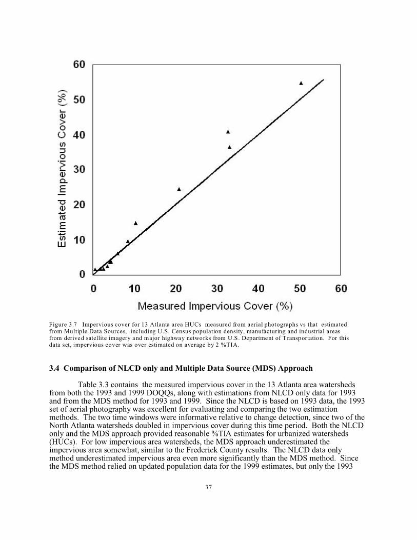
Figure 3.7 Impervious cover for 13 Atlanta area HUCs measured from aerial photographs vs that estimated from Multiple Data Sources, including U.S. Census population density, manufacturing and industrial areas from derive d satellite im agery a nd m ajor highwa y netwo rks from U.S . Dep artme nt of T ransp ortatio n. For this data set, impervious cover was over estimated on average by 2 %TIA.

3.4 Comparison of NLCD only and Multiple Data Source (MDS) Approach

Table 3.3 contains the measured impervious cover in the 13 Atlanta area watersheds from both the 1993 and 1999 DOQQs, along with estimations from NLCD only data for 1993 and from the MDS method for 1993 and 1999. Since the NLCD is based on 1993 data, the 1993 set of aerial photography was excellent for evaluating and comparing the two estimation methods. The two time windows were informative relative to change detection, since two of the North Atlanta watersheds doubled in impervious cover during this time period. Both the NLCD only and the MDS approach provided reasonable %TIA estimates for urbanized watersheds (HUCs). For low impervious area watersheds, the MDS approach underestimated the impervious area somewhat, similar to the Frederick County results. The NLCD data only method underestimated impervious area even more significantly than the MDS method. Since the MDS method relied on updated population data for the 1999 estimates, but only the 1993

37

commercial/industrial area land cover contribution, there was a somewhat greater underestimate for 1999 using the MDS method. By contrast, the MDS approach appeared to slightly over­estimate the imperviousness in the very-developed, mid-town Atlanta watersheds (HUCs).

Table 3.3 Percent Total Impervious Area (%TIA) Results for North Georgia Watersheds

HUC number DOQQ 1993

NLCD 1993

Multiple Data Sources-1993

DOQQ 1999

Multiple Data Sources-1999

031300011204 52.1 44.9 54.9 49.1 58.1

031300011202 35.8 31.6 36.6 32.3 38.0

031300011201 33.8 31.8 41.0 34.1 44.8

031300011002 8.6 6.5 9.7 15.8 13.8

031300011001 6.1 3.4 6.2 9.5 7.9

031300010907 21.0 20.7 24.6 24.4 27.6

031300010906 10.5 11.3 14.9 22.4 23.9

031501040301 1.6 1.9 1.6 2.0 1.7

031501040302 3.4 1.9 1.7 5.1 1.9

031501040303 3.7 1.9 2.5 5.5 2.9

031501040304 3.6 2.0 3.6 7.9 4.4

031501040305 5.4 2.0 3.8 8.4 4.9

031501040306 2.0 1.8 1.7 3.9 1.7

Impervious cover was subsequently estimated for 1624, 12 digit watersheds (HUCs) wholly contained within the state of Georgia, using both the simple NLCD-only approach and the MDS approach. The use of NLDC data with the ATtILA landscape factor extension tool provided a very rapid analysis and identified most of the potentially degraded watersheds (Table 3.4). The NLCD-only method identified 69 watersheds as having over 10% TIA whereas the MDS approach identified 80. The NLCD-only method under estimated the number of watersheds in the at-risk, 5 to 10 % TIA, range. For 1993, the MDS approach identified 117 HUCs in the 5 to 10% impervious class versus 76 for the NLCD only approach--35% fewer.

38

Table 3.4 Evaluation of Impervious Cover Status of Georgia Watersheds/HUC’s.

ImperviousCover Class

(% TIA)

NLCD Data Only (1993)

(# ofwatersheds)

Multiple Data Sources (1993)(# of

watersheds)

Multiple Data Sources (1999)(# of

watersheds)

Change(1993-1999)from lower to higher class*

High %TIA Growth Rate > 0.2 %TIA/

year (# of watersheds)

0 -5 1479 1427 1395 -32 12

5 - 10 76 117 137 +32 19

10 - 25 58 62 67 +12 36

> 25 11 18 25 +7 13 * Note: Since 7 HUC's moved from the 10-25 class to the >25 class between 1993 and 1999, this would leave 55 HU C's (62 - 7) in the 10 to 25 class; how ever, during the sam e time period 12 H UC 's moved from the 5 to 10 class to the 10 to 25 class for a total of 67 (1999 MDS). The calculation for movement from the 0 to 5 class to the 5 to 10 class is sim ilar.

Thus, the NLCD-only approach appears to have the most serious limitations for identifying imperviousness in the 5 to 10% range. This range, particularly in areas with significant growth, likely incorporates the most critical areas where prevention of storm water problems might be most effective. Figure 3.8 identifies for 1993 the specific Georgia HUCs categorized by MDS as ‘of concern’ (i.e. >5 %TIA) that were not identified by the NLCD-only. It is important to remember that the MDS approach may underestimate these HUCs somewhat as well.

Between 1993 and 1999, we estimated that a total of 51 HUCs changed to a higher risk impervious cover category. Figure 3.9 shows that the majority of these watersheds were in the Atlanta area. The largest change was 32 HUCs moving from the 0 to 5% class to the 5 to 10% class. Appreciable imperviousness changes were also evident in the higher impervious classes, with 12 HUCs moving from the 5 to 10% range to the 10 to 25% range and 7 HUCs from the 10 to 25% to the >25% range. For 1999, we estimated that there were a total of 229 HUCs of concern, i.e. HUCs that are currently impaired or likely to be in the near future (14% of 1624): 92 (~6%) for likely existing impairment (imperviousness above 10%), and 137 (~8%) for likely impairment in the near future (5 to 10% impervious range) if appropriate planning and management is not undertaken. The expected result is increasing storm water hydrologic, pollutant and habitat degradation stress on the streams in these areas.

39

Figure 3.8 Estimated 1993 %TIA for 1624 Georgia 12 digit HUCs. Fifty-two (52) HUCs identified as at-risk (5-10% impervious) or potentially degraded (>10% impervious) using M ultiple Data Sources (MDS), but not identified using the land cover data alone, are outlined.

40

Figure 3.9 Estimated 1999 %TIA for 1624 Georgia 12 digit HUCs. The 51 HUCs that changed to a higher risk impervious class between 1993 and 1999 are outlined.

41

4. Impervious Cover in the Southeastern United States

This section contains the estimated impervious cover results for U.S. EPA Region 4 in 2000 using the Multiple Data Source approach described in Section 3. Headquartered in Atlanta, Georgia, U.S. EPA Region 4 includes Alabama, Florida, Georgia, Kentucky, Mississippi, North Carolina, South Carolina and Tennessee. The Southeastern U.S. is one of the fastest growing areas of the country, with Florida, Georgia and North Carolina in the top ten growth states.

The major centers of population in the South are expanding, putting stress on all its ecosystems, but this sprawl is especially harmful to coastal areas, wetlands and mountains. Just 10% of the earth’s land surface holds the overwhelming majority of the earth’s population along or near coasts, and the United States is no exception. The Southeastern United States is growing rapidly along its coasts. Over 20 million people live in 99 coastal counties along the U.S. Gulf Coast (some of which are outside our study area). Florida’s burgeoning population is clearly evident, with the highest density along its eastern coast, but with significant population expansion from Tampa southward along the western coast.

Using the Multiple Data Source Approach, Figure 4.1 shows the estimated impervious cover by 12 or 14 digit HUC (depending on the individual states) for the year 2000 for the eight Southeastern states. It is easy to see the growth around the cities and interstate corridors, especially the Interstate 85 corridor from Atlanta to the Raleigh-Durham-Chapel Hill, North Carolina area. The urban intensity along the Florida east coast is also particularly evident.

Table 4.1 summarizes estimated %TIA for 2000 by state for five %TIA categories, providing a quick reference for each category for each Southeastern state. Streams in watersheds with > 20 %TIA are seriously degraded, and even the most intensive remediation efforts are likely to only partially restore functionality of those water bodies. While streams in the 10 to 20 %TIA category are also likely to suffer significant degradation from urbanization, remediation efforts can potentially restore functionality to these streams. Streams in watersheds with 5 to 10 %TIA suffer only modest degradation due to urbanization and can benefit substantially if careful planning and management of water resources is undertaken at that point in the development of the watershed. Table 4.1 clearly illustrates the extremes in the extent in urbanization in the Southeast. Whereas, only 0.1% of Mississippi’s land area is contained in HUCs with >20 %TIA, 7.0% of Florida’s HUCs are in this largely degraded category.

The maps for individual states (Figures 4.2 to 4.9) include labels of the Metropolitan Statistical Areas (MSAs) in the state. An MSA is a statistical definition by the U.S. Census Bureau to account for decentralized settlement and economic activity. It not only includes urbanized areas and outlying urban places, but also surrounding counties that are integrated with these urban centers as measured by substantial amounts of daily commuting, even if many of these surrounding areas have densities far too low to be classified as urban. A MSA must include at least one city with 50,000 inhabitants and a total metropolitan population of 100,000 or more. Approximately 82% of the U.S. population is contained in these MSAs (Kaiser statehealthfacts.org, 2004).

42

Table 4.1 % TIA as a Percentage of the Total Land Area of Each Southeastern State Using the 2000 Census and the Multiple Data Source Approach

State

Total # of

water­sheds

Area in sq miles

>20% TIA 10-20% TIA 5-10% TIA 2-5% TIA <2% TIA

# water­sheds /

sq miles %area

# water­sheds /

sq miles %area

# water­sheds /

sq miles % area

# water­sheds /

sq miles % area

# water­sheds /

sq miles % area

Alabama 1414 52197 12 / 402

0.8 29 / 990

1.9 76 / 3112

6.0 397 / 15426

29.6 900 / 32267

61.8

Florida 1365 58373 116 / 4071

7.0 104 / 4174

7.2 160 / 7053

12.1 337 /

13818 23.7

648 / 29257

50.1

Georgia 1865 58754 49 /

1381 2.4

61 / 2369

4.0 157 / 4614

7.9 559 /

17660 30.1

1039 / 32730

55.7

Kentucky 1241 40407 11 / 315

0.8 24 / 905

2.2 91 /

2827 7.0

470 / 16244

40.2 645 /

20116 49.8

Mississippi 1114 49409 2 / 67

0.1 15 / 612

1.2 37 /

1427 2.9

222 / 10138

20.5 838 / 37165

75.2

North Carolina

1601 52662 44 /

1008 1.9

101 / 2720

5.2 177 / 5769

11.0 628 /

20479 38.9

651 / 22686

43.1

South Carolina

1031 31145 39 / 513

1.7 48 /

1232 4.0

106 / 3181

10.1 362 /

11740 37.7

476 / 14547

46.7

Tennessee 1093 42139 28 / 811

1.9 40 /

1287 3.1

76 / 2917

6.9 383 /

15885 37.7

566 / 21239

50.4

(Figures may not add up to 100% due to rounding up or down.)

43

Figure 4.1 Southeastern United States impervious cover for 2000. Impervious cover as %TIA (percent total impervious area) by 12- and 14 digit HUC using the Multiple Data Source approach. Data sources used in the calculation include 1993 NLCD commercial and industrial, 2000 Census data and U.S. DOT data for interstates and other major highways.

44

4.1 Alabama

The population of Alabama in 2000 was 4.4 million people, ranking it 23rd most populous among the 50 states (U.S. Census Bureau, 2004). The state’s population increased 10.1% in the decade 1990 to 2000, below the U.S. average of 13.1%. (U.S. Census Bureau, 2004). The metropolitan population for Alabama is 71%, below the national rate of 82% (Kaiser statehealthfacts.org, 2004).

Figure 4.2 illustrates the impervious cover estimated by 12 digit HUC for Alabama in 2000. Impervious cover calculations used the Multiple Data Source approach described in Section 3. The state’s most extensive impervious cover is in and around its largest city and a long-time industrial center in the south, Birmingham. The cities of Huntsville, Montgomery (the capital), Mobile and to a lesser degree Tuscaloosa, Florence, Gadsen and Anniston also contribute to urbanization in the state. For the most part, Alabama is very rural and contains less impervious cover than many of the other Southeastern states. As in every state, there is more impervious cover around the interstate highways, but the intensity is less than other Southeastern states.

Alabama has 1414, 12 digit HUCs, 12 of which are >20% TIA, or 0.8% of its total land area. Five of those > 20% are >30%, and are in the Birmingham and Mobile MSAs. Only onewatershed, in Birmingham, is greater than 40%TIA, at 44.7%. Alabama has 29 watersheds in the 10 to 20% TIA category, or 1.9% of its area; 76 watersheds in the 5 to 10% TIA range, 6% of its area; 397 watersheds in the 2 to 5% TIA range, or 29.6% of its area; and 900 watersheds < 2% TIA, 61.8% of its area. Although Alabama has one of the lowest %TIA in the Southeast with only 41 watersheds and 8.7% of the state >10% TIA, the fragile coastal area around Mobile has 10 HUCs greater than 10%.

45

Figure 4.2 Alabama impervious cover for 2000. Impervious cover as %TIA (percent total impervious area) by 12 digit HUC calculated using the Multiple Data Source approach. Data sources used in the calculation include 1993 NLCD commercial and industrial, 2000 Census data and U.S. DOT data for interstates and other major highways.

46

4.2 Florida

Florida is the fourth most populous state in the union with the official estimate as ofApril 1, 2003 at approximately 17.1 million, a 6.8% increase in the first three years of this century. The U.S. Census Bureau ranked nine counties in Florida among the 100 fastest growingcounties in the nation during April 1, 2000 to July 1, 2003 (U.S. Census Bureau, 2004). Duringthe 1990's Florida’s population grew by 23.5%, during the 1980's by 32.7%. Net migrationcontinues to be the predominate pattern of growth for Florida, with 10.8% of the state’s growth due to natural increase and 89.2% due to net migration (Florida OCEDR 2004).

Although one of the largest and fastest growing populations in the United States, Florida still contains low density areas of rural land dominated by agricultural uses and vast areas of wetlands. The majority of the population crowds in and around the biggest cities and along the coastal areas, providing typical sprawl problems and concerns. The metropolitan population(percentage of the population located in MSAs) for Florida is 96%, the third largest of the 50states and well above the U.S. average of 82% (Kaiser statehealthfacts.org, 2004). Florida is the only state in the Southeast with a metropolitan population greater than the U.S. average.

Figure 4.3 illustrates the impervious cover by 12 digit HUC estimated for Florida in 2000 by the Multiple Data Source approach. Florida has 1365 12 digit HUCs, 116 of which are >20 %TIA, or 7% of its area. Twenty-nine of those >20 %TIA HUCs are >40%, accounting for ~1.6% of Florida’s area, with 20 watersheds in the Miami-Ft. Lauderdale area between 45.2 and 89.7 %TIA. Out of the 87 remaining HUCs in the >20 to 40 %TIA range, all but 21 are in coastal areas or sprawl from a coastal area, accounting for ~5.3% of Florida’s area. In the 10 to 20 %TIA range, Florida has 104 HUCs, accounting for 7.2% of its area. In the 5 to 10 %TIA range, Florida has 160 HUCs, accounting for12.1% of its area. Florida has the highest total of impervious cover in the top 3 categories %TIA of our study, accounting for 26.3% of its area. In the 2 to 5 %TIA range, Florida has 337 HUCs, a vast majority in the interior, accounting for 23.7% of its area. Florida has 648 watersheds <2 %TIA, the vast majority in Northern Florida, the Everglades and the interior area just north of the Everglades that accounts for 50.1% of its area. There are no watersheds below 2 %TIA on the eastern coast of Florida. Much of Florida’s coastal cities are becoming interconnected as the population grows, endangering the fragile wetlands, coastal areas and various other water ecosystems around the state.

47

Figure 4.3 Florida impervious cover for 2000. Impervious cover as %TIA (percent total impervious area) by 12 digit HUC calculated using the Multiple Data Source approach. Data sources used in the calculation include 1993 NLCD commercial and industrial, 2000 Census data and U.S. DOT data for interstates and other major highways.

48

4.3 Georgia

Georgia’s 2000 population at 8.2 million ranks 10th in the nation. Twenty counties in Georgia ranked in the 100 fastest growing counties in the nation during April 1, 2000 to July 1, 2003. Five counties were in the national top ten with growth rates above 20% in that three year period (U.S. Census Bureau, 2004). The state’s population increased 26.4% in the decade 1990 to 2000, more than double the U.S. average of 13.1%. (U.S. Census Bureau, 2004). The population for Georgia in MSAs is 72%, below the national rate of 82% (Kaiser statehealthfacts.org, 2004). Most of Georgia’s urban population is in the 28 county metropolitan statistical area (MSA) of Atlanta. This huge MSA spreads out in all directions, making congestion and environmental concerns serious issues for the state.

Figure 4.4 illustrates the impervious cover by 12 digit HUC estimated for Georgia in 2000 by the Multiple Data Source approach. There are 1865, 12 digit HUCs in Georgia, with 49 watersheds with %TIA >20% that account for 2.4% of the area of the state. Forty of these 49 HUCs are in the Atlanta MSA. The incredible sprawl facing Atlanta area residents is readily evident in Figure 4.4. Ten of the 49 >20 %TIA HUCs have >40 %TIA. There are 61 watersheds in the 10 to 20 %TIA category, accounting for 4% of Georgia’s area. The 5 to 10 %TIA range contains 157 watersheds, accounting for 7.9% of Georgia’s area. Georgia has 14.3% of its area in the top three %TIA categories of this study. Scattered throughout the state are 559 watersheds in the 2 to 5 %TIA range, accounting for 30.1% of Georgia’s area. The remaining 1039 watersheds are in the <2 %TIA range, the majority of these are in the rural south and eastern Georgia accounting for 55.7% of its area.

49

Figure 4.4 Georgia impervious cover for 2000. Impervious cover as %TIA (percent total impervious area) by 12 digit HUC calculated using the Multiple Data Source approach. Data sources used in the calculation include 1993 NLCD commercial and industrial, 2000 Census data and U.S. DOT data for interstates and other major highways.

50

4.4 Kentucky

The 2000 Census lists Kentucky’s population at slightly more than 4 million with a 9.6% increase in the decade 1990 to 2000, well below the U.S. average of 13.1%. Migration is the keycomponent of growth in the Kentucky population, affecting the composition as well as the size of the population. Kentucky has an aging population, with the rate of decadal natural increase of it’s population decreasing by 70% since 1960 to a current value of only 6% (Price,, et al. 2004). The population in MSAs for Kentucky is 45%, nearly half the national rate of 82% (Kaiser statehealthfacts.org, 2004). Kentucky’s population is centered in the north central part of the state, with the cities of Louisville, Lexington and suburban overflow population of Cincinnati, Ohio, accounting for the majority of the metropolitan population.

Huge tracks of national forest and the eastern edge of the Eastern Kentucky Coal Field (and Cumberland Plateau), called the Pottsville or Cumberland Escarpment and formed from weathering of resistant sandstones and conglomerates, dominate the eastern portion of the state. The escarpment is stepped in south-central Kentucky because several thick, resistant sandstone layers are separated by less resistant shales. The manner in which the sandstones weather and are eroded along the escarpment results in sheer cliffs, steep-walled gorges, rock shelters, waterfalls, natural bridges and arches. The Eastern Kentucky topography and the karst topography of middle Kentucky make intensive urban development difficult.

Figure 4.5 illustrates the impervious cover by 12 digit HUC estimated for Kentucky in 2000 by the Multiple Data Source approach. There are 1241, 12 digit HUCs in Kentucky, only 11 of which are >20% TIA and account for only 0.8% of the state’s area. These 11 urban HUCs are found exclusively in Louisville and Hamilton (Cincinnati, Ohio suburb). The 10 to 20 %TIA range contains 24 watersheds and accounts for 2.2% of Kentucky’s area. There are 91 watersheds in the 5 to 10 TIA% range, accounting for 7% of Kentucky’s area. Only 10% of Kentucky land area is in our top three %TIA categories where water quality impacts due to urbanization are a concern. Scattered throughout the state are 470 watersheds in the 2 to 5 %TIA range, accounting for 40.2% of Kentucky’s area. The remaining 645 watersheds in Kentucky are in the <2 %TIA range, accounting for 49.8% of its area.

51

Figure 4.5 Kentucky impervious cover for 2000. Impervious cover as %TIA (percent total impervious area) by 12 digit HUC calculated using the Multiple Data Source approach. Data sources used in the calculation include 1993 NLCD commercial and industrial, 2000 Census data and U.S. DOT data for interstates and other major highways.

52

4.5 Mississippi

The 2000 Mississippi population is listed at approximately 2.8 million, making it theleast populated state in the Southeastern region. A 10.5% increase in population in the decade1990 to 2000 puts Mississippi’s growth rate below the U.S. average of 13.1% (U.S. Census Bureau, 2004). The metropolitan population (percentage of population in MSAs) for Mississippiis 34%, making it fourth lowest in the nation (Kaiser statehealthfacts.org, 2004). Mississippi’surban population is centered around it’s largest city, Jackson, the overflow from Memphis along its northern border, and the booming coastal area of Gulfport and Biloxi.

Figure 4.5 illustrates the impervious cover by 12 digit HUC estimated for Mississippi in 2000 by the Multiple Data Source approach. Of the 1114, 12 digit HUCs in Mississippi, only 2 are >20% TIA, accounting for only 0.1% of its area. One of these >20 %TIA watersheds is located in the Jackson MSA with 38.6 %TIA, and the other is located along the Gulf Coast with 22.1 %TIA. Even the next category, the 10 to 20 %TIA range, only contains 15 watersheds, accounting for 1.2 % of Mississippi’s area. There are 37 watersheds in the 5 to 10 %TIA range, accounting for 2.9 % of Mississippi’s area. In the 2 to 5 %TIA range, Mississippi has 222 watersheds, accounting for 20.5% of Mississippi’s area. The remaining 838 watersheds in Mississippi are in the <2 %TIA range, accounting for 75.2% of its area. Mississippi has thelowest impervious cover of all the Southeastern states, with only 4.2% of its area in the top three categories of %TIA. Unfortunately, approximately 90% of the area in the fragile ecosystems of the Gulf Coast are in the top three categories of impervious cover (>5%) of this study.

53

Figure 4.6 Mississippi impervious cover for 2000. Impervious cover as %TIA (percent total impervious area) by 12 digit HUC calculated using the Multiple Data Source approach. Data sources used in the calculation include 1993 NLCD commercial and industrial, 2000 Census data and U.S. DOT data for interstates and other major highways.

54

4.6 North Carolina

The North Carolina 2000 population was slightly more than 8 million, with a 21.4% increase in the decade 1990 to 2000, well above the U.S. average of 13.1%. Five counties in North Carolina ranked in the 100 fastest growing counties in the nation during April 1, 2000 to July 1, 2003 (U.S. Census Bureau, 2004). The metropolitan population (percentage of thepopulation living in MSAs) for North Carolina is 70%, below the national rate of 82% (Kaiser statehealthfacts.org, 2004). The majority of the North Carolina population is concentrated in themiddle of the state, in clusters around their major metropolitan statistical areas–Charlotte-Gastonia-Rock Hill, Raleigh-Durham-Chapel Hill, Greensboro-Winston-Salem-High Point and Fayetteville. The western portion of North Carolina is mountainous and the eastern portion is coastal, making North Carolina attractive for second homes, retirement and seasonal housing. North Carolina was fourth in the nation in adding persons 65 and older to its numbers April 1, 2000 to July 1, 2003 (U.S. Census Bureau, 2004).

Figure 4.7 illustrates the state’s impervious cover by 12 digit HUC estimated for 2000 using the Multiple Data Source approach. This figure clearly shows the extensive development around its MSAs in the central part of the state and along Interstates 85 and 40. There are 1601, 14 digit HUCs in North Carolina, 44 of which are >20 %TIA, accounting for 1.9% of its area. There are 101 watersheds 10 to 20 %TIA accounting for 5.2% of North Carolina’s area. The 5 to 10 %TIA range contains 177 watersheds, accounting for 11% of its area. There are 628 watersheds in the 2 to 5 %TIA range, accounting for 38.9% of North Carolina’s area. The remaining 651 watersheds are in the <2 %TIA range, accounting for 43.1% of its area, the lowest amount for any Southeastern state. Although North Carolina does not have an extremely high number of watersheds in the highest %TIA category, it does have a relatively high percentage of its land area, 18.1%, in the top three %TIA categories, making it second highest in the Southeast.

55

Figure 4.7 North Carolina impervious cover for 2000. Impervious cover as %T IA (percent total impervious area) by 14 digit HUC calculated using the Multiple Data Source approach. Data sources used in the calculation include 1993 NLCD commercial and industrial, 2000 Census data and U.S. DOT data for interstates and other major highways.

56

4.7 South Carolina

The South Carolina 2000 population was 4 million, with a 15.1% increase in the decade1990 to 2000, just slightly above the U.S. average of 13.1%. The metropolitan population(percentage of the population in MSAs) for South Carolina is 75%, below the national rate of 82% (Kaiser statehealthfacts.org, 2004). South Carolina’s population is much like the otherSouthern states, expanding out from its biggest metropolitan area, the Anderson-Greenville-Spartanburg MSA, along the Interstate 85 corridor. Other areas of growth in South Carolina include its capitol, Columbia, and the coastal port of Charleston.

Figure 4.8 illustrates the South Carolina impervious cover by 14 digit HUC estimated for 2000 using the Multiple Data Source approach. South Carolina has 1031, 14 digit HUCs, 39 of which are >20% TIA, representing 1.7% of its land area. Eighteen of those >20 %TIA are >30 %TIA and are located in Columbia, the Greenville-Spartanburg-Anderson MSA and in the Atlantic coastal area. South Carolina has 48 watersheds in the 10 to 20% TIA range, representing 4% of its land area; 106 watersheds in the 5 to 10% TIA range, or 10.1% of its area. South Carolina’s total area in our top three %TIA categories is 15.8%, third highest in the Southeast. South Carolina’s 362 watersheds in the 2 to 5% TIA range account for 37.7% of its area, and the 476 watersheds <2 %TIA account for 46.7% of its area.

57

Figure 4.8 South Carolina impervious cover for 2000. Impervious cover as %TIA (percent total impervious area) by 14 digit HUC calculated using the Multiple Data Source approach. Data sources used in the calculation include 1993 NLCD commercial and industrial, 2000 Census data and U.S. DOT data for interstates and other major highways.

58

4.8 Tennessee

The Tennessee 2000 population was 5.7 million, with a 21.4% increase in the decade 1990 to 2000, about 60% greater than the U.S. average of 13.1%. The metropolitan population(percentage of the population residing in MSAs) for Tennessee was 69%, below the national rate of 82% (Kaiser statehealthfacts.org, 2004). The majority of the population in Tennessee is centered around Memphis in the southwestern corner of the state, Nashville in central Tennessee, and in the eastern portion of the state from Chattanooga to Knoxville and along a corridor stretching along Interstates 75, 40 and 81 to Bristol, Tennessee at the Virginia border.

Figure 4.9 illustrates the estimated Tennessee impervious cover by 12 digit HUC for 2000 using the Multiple Data Source approach. Tennessee has 1093, 12 digit HUCs, 28 of which are >20% TIA, or 1.9% of its area; 40 watersheds 10 to 20% TIA, or 3.1% of its area; 76 watersheds 5 to 10% TIA, or 6.9% of its area; 383 watersheds 2 to 5% TIA, or 37.7% of its area; and 566 watersheds < 2% TIA, or 50.4% of its area. Tennessee has 11.9% of its total land area in the top three %TIA categories of this study.

59

Figure 4.9 Tennessee impervious cover for 2000. Impervious cover as %TIA (percent total impervious area) by 12 digit HUC calculated using the Multiple Data Source approach. Data sources used in the calculation include 1993 NLCD commercial and industrial, 2000 Census data and U.S. DOT data for interstates and other major highways.

60

5. Future Impervious Cover Projections for the Southeastern United States

According to the Census Bureau population projections, several states in the Southeastern United States will be among the fastest growing of the country in the next three decades. EPA’s Region 4 contains two states, Florida and Georgia, that are expected to have the third and fourth largest population increase between 1995 and 2025 in the nation (Campbell, 1997). Florida is expected to add over six million additional residents while Georgia and North Carolina areexpected to add over two million. Mississippi and Kentucky are projected to show the slowest net population growth, adding just under ½ million individuals. Coastal areas will generally show the greatest growth, with slower growth in the inland areas.

Along with this population growth will inevitably come an increase in impervious cover. In this section projections of impervious cover in the12 and 14 digit HUCs are made based on county scale population projections obtained from the individual states combined with the Multiple Data Source impervious cover estimation method discussed in Sections 3 and 4. These projections represent a single scenario of a possible distribution of impervious cover in the eightSoutheastern states and should be used in this context. Included is a discussion of error estimates of population projections upon which the imperviousness is based to give the reader a sense of the magnitude of error associated with these projections.

5.1 The Nature of Errors in Population Projections

Estimates of potential error for population projections are not done routinely among the community of demographers (Smith 1987). Such estimates are particularly desirable for this impervious estimation study, however, since population is the key driving component of the impervious area projections and estimates. Several existing population projection error studies were surveyed to establish a basis for potential errors associated with impervious estimates and projections. These studies spanned several spatial scales including: state, county and sub-county areas. Population projection error estimates at all these scales are summarized here and used in to illustrate the likely bounds of potential impervious area estimates based largely on population projections.

Smith and Sincich (1992) carried out a comprehensive retrospective evaluation of state level population projection errors using an array of simple extrapolation approaches compared to each other and to more complex models. They evaluated the accuracy of state population projections for the 1960’s, 70’s and 80’s using: linear extrapolation (LINE); exponential extrapolation (EXPO); a moving average time series model (ARIMA); ratio techniques including shift-share (SHIFT), which assumes that a state’s share of national population changes “...by the same annual amount during the projection horizon as the average annual change during the base period,” and share of growth (SHARE), which assumes that “...each state’s share of national population growth during the projection horizon is the same as during the base period.” Othermore complex models evaluated included those of the Census bureau, the National PlanningAssociation, and the Bureau of Economic Analysis. The measures of error that they evaluated included: mean absolute percent error (MAPE), root mean square percent error (RMSPE), 90th

percentile of absolute percent errors (90PE), Mean Algebraic Percent Error (MALPE), Percentage of positive errors (%POS)

The two best simple models were LINE and SHARE, with SHARE performing slightly better. The simple models performed as well or better than the more complex approaches (Smith & Sincich 1992). Typical MAPE ranges for these techniques were: 5 to 8% for 10 year

61

projections, and 10 to 12% for 20 year projections. Thirty (30) year projections were not evaluated. Here we assume that a reasonable MAPE for 30-year projections at the State level might be in the range 15 to 18%. This “guess”, however, is based only on limited experience and best professional judgement and no hard data. Clearly, additional research is needed to establish potential error for long term population projections over 20 years.

The U.S. Bureau of the Census and others, especially users of population projections, are becoming increasingly interested in consistent, regular, sound evaluation of population projection error. Campbell and others evaluated error in state population projections using Census 2000 counts. They found that short term projections up to 5 years might expect MAPE’s of about 0.5% per year at the state level (Campbell, et al. 2002). These values are consistent with the results of Smith and Sincich (1992) discussed above.

At the county scale a similar evaluation process found “…mean absolute errors of around 15% for 10-year projections and around 30% for 20-year projections” (Smith 1987). Smith evaluated projections vs. census enumerations for 2,971 counties over the years 1950 through 1980. He observed that migration patterns dominated both increases and decreases in population and that extremely high growth rates tend to moderate over time. He also established several general characteristics of population projection accuracy:

• forecast errors increase with length of projection horizon, • larger errors are expected for places with high growth rates, • larger errors are expected for small (low population) places, and • there is no way to predict whether errors will be positive or negative.

Since the errors in population projections depend on population (size of place) and on therate of population growth, “… population forecast errors are frequently going to be large, especially for small and/or rapidly growing places” (Smith 1987). Recognizing this, Smith suggested that population projection refinements could be based on separating counties by rate of population growth (during the base period), by size of place (population) or both.

At the census tract scale a study of three diverse Florida counties found a MAPE in the range of 17 to 20% for 10-year projections (Smith and Shahidullah 1995). These authors found larger errors for smaller tracts, ~ 30 to 35% for <2,500 population over 10 years, and larger errors for larger absolute growth rates. They also tested and found the smallest errors for a composite (COMP) method where the estimation approach was tailored to population growth characteristics of each census tract. The COMP errors for census tracts by growth rate for a 10­year period were as follows:

Growth Rate COMP error

<10% ~20%10 to 25% ~10%25 to 50% ~20%>50% ~30%

Using over 40,000 sub-county areas (municipalities, townships, etc.) nationwide, Harper and others evaluated 10 year errors for projections using sub-county housing unit data to distribute county populations to sub-county areas (Harper, et al. 2003). They found that error (MAPE and MAPLE) depended on both sub-county area size (population) and growth rate.

62

MAPE for all areas was 12.4% ranging from 4.0% (population 50,000 to 100,000) to 35.1% (population < 100).

Projections of urban expansion tailored to specific locales can incorporate considerable additional complexity and potentially more accuracy relative to the simpler approaches based on population projections taken here. One example of a more detailed local projection of urban growth is that for the Charleston region of South Carolina (Allen and Lu 2003) which predicts a change in urban area from 250 square miles in 1994 to 868 square miles in 2030. This effort utilized multiple approaches including logistic regression, rule based suitability (for transition probabilities) and focus groups as the basis for an integrated future urban growth model. Comprehensive accuracy assessments of these complex localized approaches have not been done and no good guidelines exist to evaluate improvement in projection accurate as a function of this increased complexity.

5.2 Impervious Cover Projection Method

Impervious cover projections based on an Multiple Data Source approach are analogous to those described for current condition, but incorporate projected population growth as described below. Additional details of calculation and data processing can be found in the Appendix.

5.2.1 Residential Component

Although the U.S. Census Bureau prepares state level population projections for the entire nation, individual states prepare projections of population at the county scale level. Both methodology and available time period for projection vary from state to state. Some states in Region 4 have official population projections until 2030, while other states have them only until 2010 or 2015. Population projections by county for the eight Southeastern states in Region 4 were obtained from each individual state. Table 5.1 summarizes information on county scale projections for each state including the projection time period, date projections were made andorganization from which projections were obtained.

Since we are interested in projections for the 12 and 14 digit HUCs, the environmentally significant subdivision, the coarser political (county) scale projections need to be apportioned to the finer HUC scale. The first step was to apportion the growth to the 2000 census block level. With this done the population could be apportioned to the individual blocks as describedpreviously for current condition estimation of impervious cover. Two different approaches were considered to distribute county scale projections to the block level: (1) based on the most recentgrowth at the block level, i.e. proportional to block level population change between 1990 and 2000, or (2) based on the most recent block level population density. Both of these approacheshave arguable advantages and disadvantages. The first approach assumes that the recent historical level of growth will continue over the next 30 years while the second assumes that population growth will be proportional to the current population. Neither of these methods can be considered the “right” way to apportion the growth, but both can form the basis for making reasonable projections.

Basing the distribution on growth patterns in the past ten years identifies recent boom areas of a county. This method is likely to overestimate future growth for the very rapidly growing areas of the counties and to underestimate growth for areas that are currently experiencing slower growth and to continue contraction of populations unrealistically in some

63

Table 5.1 Sources and Dates of Population Projections for Each Southeastern State

State Source Date of

Projections

Years A vailab le

2005 2010 2015 2020 2025 2030

Alabama Univ. of Alabama

August2001 x x x x x

Florida Univ. of Florida July 2003 x x x x x

Georgia Gov’s. Ofc. of Planning& Budget

June 2002 x

Kentucky Univ. of

Louisville July 2003 x x x x x x

Mississippi

MS Institutes of

HigherLearning

March 2002

x x x

North Carolina

NC Ofc. of State Budget

& Mgmt. June 2003 x x x x x x

South Carolina

SC State Budget &

Control Bd.

October 2002 x x x x x

Tennessee Univ. of Tennessee

March 1999 x x x x

blocks that have had declines in population. Local peak growth or contraction areas will shift over less than the 25 year period for most of the areas. A technical difficulty in trying to use this approach is that census blocks were realigned between the 1990 and 2000 Census so determiningthe growth individual blocks presents difficulties. A commercial product which offers 1990 Census data mapped onto the 2000 block configuration was evaluated for use in this process. Unfortunately, this product shows some unrealistic expansion and contractions in some areas. Blocks around large military bases seemed to be particularly problematic but other pockets of problems also seem to exist with this data set. Some block populations are zeroed out and othershow unrealistically high increases in population between the two census periods. Doingadequate quality control with this approach for a multiple state area did not appear feasible. This approach may be possible to use for smaller multiple county areas. Due to the quality control issues with method one, projected growth in a county was distributed based on the 2000 population in the blocks. Distributing growth proportional to the 2000 population will tend to underestimate growth in rural areas of a county and overestimate growth in urban areas.

64

The population projection errors at the HUC level due to their relatively small size will be larger than county scale projection errors no matter how the population is distributed. For example, the average of the HUC population in Georgia in 2000 (based on 8.2 million people and 1865 HUCs) is only 4400 and there are an average of 12 HUCs per county in the state. Based on the error in population projection analysis [Smith (1987), Smith and Shahidullah(1995)] discussed in the previous section, smaller high growth rate HUCs could easily have projection errors in the 50% range even for a 10 year projection horizon.

The projected population density in each HUC was calculated for the projection time periods available from individual states. The projection window ranged from Georgia with projections out only to 2010, to Kentucky and North Carolina with projections out to 2030. Projections of HUC populations were made at five year intervals based on the individual state projections. The residential component of impervious cover for each time period was then calculated based on the Hicks equation as described in Section 3.

5.2.2 Commercial/Industrial Component

The critical assumption for the High Intensity Commerial/Industrial (HICI) area future projections was to maintain in a particular HUC the HICI (in square miles) /10,000 population ratio constant for future periods. This assumption would provide at least a reasonable estimate of future HICI change due to population growth since the commercial/industrial contribution to %TIA contains a major component that is proportional to the population density in the nearbyarea, i.e. commercial areas that serve the residents of an area. Figure 5.1 illustrates the relationship between population and the High Intensity Commercial/Industrial class for North Carolina HUC’s for the single time period -- 1993 -- when the categorized land cover data was available.

The above assumption reflects both the linear nature and the dispersion of the relation­ship between HICI area and population. The implications of this assumption for the projectionare that the historical pattern of commercial growth with respect to population for any particular area (HUC) will continue into the projection periods. Thus, areas with high HICI/population ratios are projected to experience high commercial growth with population increases, areas with low HICI/population ratios are projected to experience low commercial growth with population increases, and those areas with intermediate ratios will be in between. Actual future change of HICI area with population for any individual HUC could differ from this assumption, but lackinghistorical change information for the HICI/population ratio, we consider this “space for time” substitution approach for the assumption to be objective and sensible based on the available data. As future coincident commercial/industrial area and population data become available, including an updated NLCD for 2000, future censuses and other appropriate data, the actual reliability of this assumption should be tested and evaluated.

65

Figure 5.1 H igh Inten sity Com merc ial/Indu strial area (mete rs) vs. po pulatio n for N orth C arolina 12 d igit HU C’s

For the majority of HUCs, the projection was made as follows:

ComTIA%[period] = ((Comm_area[1993] * Bpop[period]) / HUC_area) * 0.90 * 100 Bpop_93

Where:

Comm_area[1993] = NLCD HICI of HUC for 1993Bpop_93 = population of HUC for 1993

(interpolated between 1990 & 2000)Bpop[period] = population of HUC for projected period

(2000, 2010, 2020 & 2030)HUC_area = area of HUC in square miles0.90 = assumed fraction of TIA for HICI class of NLCD

and ComTIA%[period] = commercial/industrial component of TIA for projected period

However, a major industrial component in this category can be relatively independent of the surrounding residential population, i.e., large manufacturing or transportation facilities may be located at a distance from local population centers. In addition, if population declines in an area the impervious area does not tend to decline.

66

Two constraints were implemented to maintain realistic ranges and distribution of variability in future projections of the HICI (High Intensity Commercial/Industrial) TIA component. First, decreases of HICI (High Intensity Commercial/Industrial area) for future time periods are not considered likely and are not allowed, i.e.:

IF HICI(future period) < HICI(1993) THEN HICI(future period) = HICI(1993)

Second, increases of HICI were also limited to constrain potential large increases in future periods for outliers (HUCs with large HICI/population ratios) that could unrealistically increase HICI area with only small population increases. North Carolina was used as a case study to establish a reasonable range for this ratio. We identified 57 HUC’s: 3.6 % of the 1601 HUC’s statewide, that had HICI/population ratios above 3 square miles per 10,000 population. We consider these to be out of the typical range. The unusual high ratio areas examined evidenced a wide array of circumstances including, for example: low population with a coastal causeway or rural interstate classified as commercial/industrial, low population with a large rural industrial facility, airport, mine or other facility classified as commercial/industrial.

This constraint was implemented with the IF-THEN construction:IF HICI(in square miles for 1993)/10Kpopulation(1993) > 3.0

....THEN HICI(future period) = HICI(1993) + Median HICI Change

Where: Median HICI Change = 0.6 square mile * ((Population(period2) - Population(period1))/10,000

This constant is based on the median HICI area per 10,000 population ratio of all HUCs statewide in North Carolina. (The mean ratio was 0.7.)

5.2.3 Major Highway Component

The only roadways included in this component were interstate highways and major US highways. This is a minor component in the impervious cover estimation and very little new connector highway construction is proposed. Projected construction information is in a variety of formats and not easily obtainable from individual states. Since updated values will have anegligible effects on projections, estimates of current status described in Chapter 4 was used in projection estimates.

5.3 Impervious Cover Projections

The West and the South are projected to have the greatest net population change over the next three decades in the nation. All of the states in the Southeast are expected to increase in population in the following decades with Florida and Georgia leading the growth. Florida is expected to replace New York as the third (behind California and Texas) most populous state by 2020 (Campbell, 1997). Population projections from each of the eight Southeastern states in EPA Region 4 are show in Table 5.2 and form the basis for the impervious cover projections for each state of the eight states detailed below.

67

--

--

-- -- -- -- --

-- -- --

--

-- --

Table 5.2 2000 U.S. Census and State Population Projections for the Southeastern United Statesin Thousands

State 2000 Population

2005 Population

2010 Population

2015 Population

2020 Population

2025 Population

2030 Population

Alabama 4,447 4,645 4,839 5,028 5,211 5,386

Florida 15,982 17,499 18,978 20,387 21,807 23,178

Georgia 8,186 9,592

Kentucky 4,042 4,183 4,321 4,447 4,563 4,663 4,744

Mississippi 2,845 2,991 3,118 3,227

North Carolina

8,049 8,784 9,491 10,227 10,966 11,712 12,448

South Carolina

4,012 4,155 4,388 4,618 4,850 5,077

Tennessee 5,689 5,798 6,063 6,327 6,593

68

5.3.1 Alabama

In the 2000 Census Alabama was the 22nd most populous state with 4.4 million people and is not expected to change its ranking significantly among the 50 states and District of Columbia in the next 25 years (U.S. Census Bureau, 2001a and b). Overall, growth will bemoderate with the population projected to grow by just under 1 million people reaching 5.4 million people by 2025, an increase of 21% over a 25 year period (Campbell, 1997).

Although overall population increase is projected to be less than 1% per year over the next two decades, some counties are projected to grow much more rapidly while some will show a decline in population. Shelby County, located in the Southeastern portion of the BirminghamMSA is projected to add over 120,000 people, a percentage increase of 85% or over 3% annual growth rate. Baldwin County located on the Gulf Coast on the eastern side of the Mobile MSA is projected to add over a 100,000 people with a 77% increase over the 25 year period. Five other counties (Autauga, Blount, Elmore, Lee, and St.Clair) are expected to show an increase in population of over 50% by 2025. These counties are located on the outskirts of existingpopulation centers including Birmingham, Montgomery and Auburn. At the other end of the spectrum, several rural counties distant from major population centers are projected to decline in population. The population projections by county for the state of Alabama were obtained from the Center for Business and Economic Research, University of Alabama. The projections, available out to 2025, were published in August 2001. Projections in this series are based on trends between the 1990 and 2000 censuses.

Figure 5.2 shows the impervious cover projections for Alabama watersheds calculated using the Multiple Data Source approach described in Section 4 and Section 5.2. The number of HUCs and percentage land area in each impervious cover class are summarized in Table 5.3 with the pattern of percent area by TIA class shown in Figure 5.3 The number of stream miles in each %TIA category is summarized in Table 5.4 with the pattern of stream miles by TIA class shown in Figure 5.4.

The increase in impervious cover between 2000 and 2025 can be seen in the far south Gulf Coast and around the other urban centers. Figure 5.3 shows a drop in the area of HUCs with <2% impervious and increases in the other four classes. In 2000, 2.7 % of the land area (1409 mi2) was in HUCs with %TIA > 10% (areas where stream quality is likely degraded). By2025, 3.5% of the land area (1827 mi2) was in HUCs with %TIA > 10%. By 2025, 3.0 % (2294 mi) of Alabama streams are projected to be in HUCs with %TIA > 10% while 91 % (70,116 mi) are in areas not immediately threatened by urbanization with < 5% impervious area.

69

Figure 5.2 Alabama projected impervious cover out to 2025. Impervious cover as %TIA (percent total impervious area) by 12 digit HUC calculated using the Multiple Data Source approach. Data sources used in the calculation include 1993 NLCD commercial and industrial cover, 2000 Census data, county level population projections from University of Alabama and U.S. DOT data for interstates and other major highways.

70

Table 5.3 %TIA as a Percentage of the Total Land Area of Alabama out to 2025

Year

>20% TIA 10-20% TIA 5-10% TIA 2-5% TIA <2% TIA

# HUCs

% area

# HUCs

% area

# HUCs

% area

# HUCs

% area

# HUCs

% area

2000 12 0.8 29 1.9 76 6.0 397 29.6 900 61.8

2010 15 1.0 31 2.0 78 6.2 430 31.8 860 59.0

2020 19 1.3 31 2.1 90 7.0 435 32.2 839 57.5

2025 21 1.4 31 2.1 92 7.0 443 32.7 827 56.8 Total number of HUCs: 1414 Total area: 52,197.5 sq mi

Figu re 5.3 Alabama Projected %TIA as % of Area out to 2025

71

Table 5.4 Total River Miles in Alabama by %TIA category out to 2025

Year

>20% TIA 10-20% TIA 5-10% TIA 2-5% TIA <2% TIA

# HUCs

river miles

# HUCs

river miles

# HUCs

river miles

# HUCs

river miles

# HUCs

river miles

2000 12 420 29 1225 76 4320 397 21654 900 49769

2010 15 579 31 1314 78 4452 430 23472 860 47572

2020 19 783 31 1329 90 5049 435 23815 839 46411

2025 21 882 31 1412 92 4977 443 24216 827 45900 Total number of HUCs: 1414 Total river miles: 77,389

Figure 5.4 Total River Miles in Alabama by %TIA Category out to 2025

72

5.3.2 Florida

Florida is currently the 4th most populous state in the U.S. with nearly 16 million people counted in the 2000 census (U.S. Censure Bureau, 2001). According to the U.S. Census Bureau, Florida is projected to replace New York as the 3rd most populous state in the union and by 2025the population is projected to grow to 20.7 million people (Campbell, 1997). The University of Florida Population Program, on the other hand, projects even more rapid growth for the state with a total of 23.2 million people by 2025 (Smith and Nogle, 2003). These projections refersolely to permanent residents and do not include tourists or seasonal residents, a major category in some areas of Florida. Florida is a highly diverse state and growth is not distributed evenly. While some areas have grown rapidly, others have grown slowly or even declined in population.

Rapid growth is expected along the northeastern Atlantic coast with St. Johns (St. Augustine area) and Flagler County (south of St. Augustine) doubling in population between 2000 and 2025. Sumter County (southwest of Ocala) is projected to double in population while Marion County located west of Ocala will nearly double as well. Collier County on the Gulf Coast south of Fort Meyers is also expected to double in population. Miami-Dade is expected to add 800,000 more people, with its population reaching 3.1 million by 2025. Counties surrounding Orlando are expected to grow rapidly as well. Some rural areas of the state such as the area south and east of Tallahassee will experience slow or no growth.

The population projections by county for the state of Florida were obtained from the Bureau of Economic and Business Research, Warrington College of Business Administration, University of Florida, Gainesville, Florida. The projections, available out to 2025, werepublished July 2003. These county scale projections served as the basis for the projection of future impervious cover for the state of Florida

Figure 5.5 shows the impervious cover estimations and projections for Florida watersheds calculated using the Multiple Data Source approach described in Section 4 and Section 5.2. The number of HUCs and percentage land area in each impervious cover class are summarized in Table 5.5 with the pattern of percent area by TIA class shown in Figure 5.6. The number of stream miles in each %TIA category is summarized in Table 5.6 with the pattern of stream miles by TIA class shown in Figure 5.7.

In 2000, 14.2 % of the land area (8289 mi2) was in the 220 HUCs with %TIA > 10%(areas where stream quality is likely degraded). By 2025, 21.3% of the land area (12434 mi2)was projected to be in the 298 HUCs with %TIA > 10%. By 2025, 26% (15341 mi) of Florida streams are projected to be in HUCs with %TIA > 10% while 63% (36598 mi) are in areas not immediately threatened by urbanization with < 5% impervious area. Between 2000 and 2025, 4900 more miles of streams, a 45% increase, will be located in watersheds likely to suffer serious degradation due to development (>10 %TIA) unless advanced planning and mitigation efforts are undertaken soon. These watersheds are located along both the Atlantic and Gulf coastal areas and in the central Florida expanding east and southwest of Orlando.

73

Figure 5.5 Florida projected impervious cover out to 2025. Impervious cover as %TIA (percent total impervious area) by 12 digit HUC calculated using the Multiple Data Source approach. Data sources used in the calculation include 1993 NLCD commercial and industrial cover, 2000 Census data, county level population projections from University of Florida and U.S. DOT data for interstates and other major highways.

74

Table 5.5 % TIA as a Percentage of the Total Land Area of Florida out to 2025

Year

>20% TIA 10-20% TIA 5-10% TIA 2-5% TIA <2% TIA

# HUCs

% area

# HUCs

% area

# HUCs

% area

# HUCs

% area

# HUCs

% area

2000 116 7.0 104 7.2 160 12.1 337 23.7 648 50.0

2010 133 7.9 127 8.6 142 11.4 351 25.2 612 47.0

2020 142 8.5 144 10.1 142 11.4 352 25.0 585 45.1

2025 152 9.6 146 11.7 147 9.9 342 24.1 578 44.7

Total number of HUCs: 1365 Total area: 58,376.2 sq mi

Figure 5.6 Florida Projected %TIA as % of Area out to 2025

75

Table 5.6 Total River Miles in Florida per TIA category out to 2025

Year

>20% TIA 10-20% TIA 5-10% TIA 2-5% TIA <2% TIA

# HUCs

river miles

# HUCs

river miles

# HUCs

river miles

# HUCs

river miles

# HUCs

river miles

2000 116 5346 104 5101 160 8034 337 12008 648 27462

2010 133 5787 127 6398 142 7025 351 13357 612 25384

2020 142 6090 144 6885 142 7870 352 12536 585 24569

2025 152 7048 146 8293 147 6011 342 12209 578 24389 Total number of HUCs: 1365 Total river miles: 57,953

Figure 5.7 Total River Miles in Florida by %TIA Category out to 2025

76

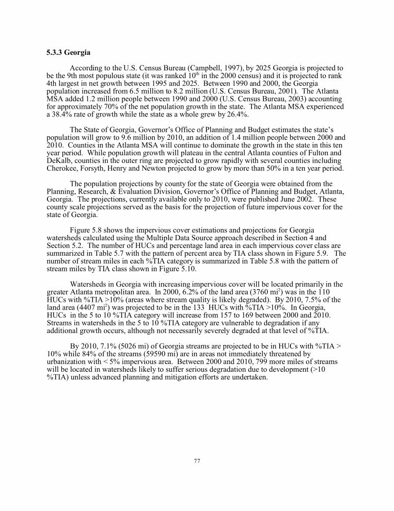
5.3.3 Georgia

According to the U.S. Census Bureau (Campbell, 1997), by 2025 Georgia is projected to be the 9th most populous state (it was ranked 10th in the 2000 census) and it is projected to rank4th largest in net growth between 1995 and 2025. Between 1990 and 2000, the Georgia population increased from 6.5 million to 8.2 million (U.S. Census Bureau, 2001). The Atlanta MSA added 1.2 million people between 1990 and 2000 (U.S. Census Bureau, 2003) accounting for approximately 70% of the net population growth in the state. The Atlanta MSA experienceda 38.4% rate of growth while the state as a whole grew by 26.4%.

The State of Georgia, Governor’s Office of Planning and Budget estimates the state’s population will grow to 9.6 million by 2010, an addition of 1.4 million people between 2000 and 2010. Counties in the Atlanta MSA will continue to dominate the growth in the state in this tenyear period. While population growth will plateau in the central Atlanta counties of Fulton andDeKalb, counties in the outer ring are projected to grow rapidly with several counties including Cherokee, Forsyth, Henry and Newton projected to grow by more than 50% in a ten year period.

The population projections by county for the state of Georgia were obtained from the Planning, Research, & Evaluation Division, Governor’s Office of Planning and Budget, Atlanta, Georgia. The projections, currently available only to 2010, were published June 2002. These county scale projections served as the basis for the projection of future impervious cover for the state of Georgia.

Figure 5.8 shows the impervious cover estimations and projections for Georgia watersheds calculated using the Multiple Data Source approach described in Section 4 and Section 5.2. The number of HUCs and percentage land area in each impervious cover class are summarized in Table 5.7 with the pattern of percent area by TIA class shown in Figure 5.9. The number of stream miles in each %TIA category is summarized in Table 5.8 with the pattern of stream miles by TIA class shown in Figure 5.10.

Watersheds in Georgia with increasing impervious cover will be located primarily in the greater Atlanta metropolitan area. In 2000, 6.2% of the land area (3760 mi2) was in the 110HUCs with %TIA >10% (areas where stream quality is likely degraded). By 2010, 7.5% of the land area (4407 mi2) was projected to be in the 133 HUCs with %TIA >10%. In Georgia, HUCs in the 5 to 10 %TIA category will increase from 157 to 169 between 2000 and 2010. Streams in watersheds in the 5 to 10 %TIA category are vulnerable to degradation if any additional growth occurs, although not necessarily severely degraded at that level of %TIA.

By 2010, 7.1% (5026 mi) of Georgia streams are projected to be in HUCs with %TIA > 10% while 84% of the streams (59590 mi) are in areas not immediately threatened by urbanization with < 5% impervious area. Between 2000 and 2010, 799 more miles of streams will be located in watersheds likely to suffer serious degradation due to development (>10 %TIA) unless advanced planning and mitigation efforts are undertaken.

77

Figure 5.8 Georgia impervious cover out to 2010. Impervious cover as %TIA (percent total impervious area) by 12 digit HUC calculated using the Multiple Data Source approach. Data sources used in the calculation include 1993 NLCD commercial and industrial cover, 2000 Census data, county level population projections from Georgia Governor’s Office of Planning & Budget and U.S. DOT data for interstates and other major highways.

78

Table 5.7 % TIA as a Percentage of the Total Land Area of Georgia

Year

>20% TIA 10-20% TIA 5-10% TIA 2-5% TIA <2% TIA

# HUCs

% area

# HUCs

% area

# HUCs

% area

# HUCs

% area

# HUCs

% area

2000 49 2.4 61 4.0 157 7.9 559 30.1 1039 55.7

2010 58 2.8 75 4.7 169 8.3 579 31.2 984 53.0 Total number of HUCs: 1865 Total area: 58,754.1

Figure 5.9 Georgia Projected %TIA as % of Area out to 2010

79

Table 5.8 Total River Miles in Georgia per TIA category

Year

>20% TIA 10-20% TIA 5-10% TIA 2-5% TIA <2% TIA

# HUCs

river miles

# HUCs

river miles

# HUCs

river miles

# HUCs

river miles

# HUCs

river miles

2000 49 1464 61 2763 157 5833 559 22671 1039 38235

2010 58 1735 75 3291 169 6350 579 23599 984 35991 Total number of HUCs: 1865 Total river miles: 70,966

Figure 5.10 Total River Miles in Georgia by %TIA Category out to 2010

80

5.3.4 Kentucky

According to the U.S. Census Bureau (Campbell, 1997), Kentucky is projected to be one of the slowest growing states in the nation between 1995 and 2025. A landlocked state at the northern edge of Region 4, Kentucky’s growth patterns are likely to be more similar to its midwestern neighbors to the north and west than the booming South Atlantic states. The University of Louisville, Urban Studies Institute (2003) projects an increase in Kentucky’s population from 4.0 million in 2000 to 4.7 million in 2030. Growth in the state will occur primarily around Lexington, Louisville, and in the suburban areas south of Cincinnati, OH.

Population projections by county for the state of Kentucky were obtained from the Kentucky State Data Center, University of Louisville, Urban Studies Institute, Louisville, Kentucky http://ksdc.louisville.edu/kpr/pro/pro2002.htm. The projections, available out to 2030,were published July 2003.

Figure 5.11 shows the impervious cover estimations and projections for Kentucky watersheds calculated using the Multiple Data Source approach described in Section 4 and Section 5.2. The number of HUCs and percentage land area in each impervious cover class are summarized in Table 5.9 with the pattern of percent area by TIA class shown in Figure 5.12. The number of stream miles in each %TIA category is summarized in Table 5.10 with the pattern of stream miles by TIA class shown in Figure 5.13.

Inspection of Figure 5.11 shows relatively little change between 2000 and 2030. In 2000, 3.0 % of the land area (1212 mi2) were in the 35 HUCs with %TIA >10% (areas where stream quality is likely degraded). By 2030, 3.7% of the land area (1495 mi2) was projected to be in the42 HUCs with %TIA >10%. HUCs in the 5 to 10 %TIA category will increase from 91 to 105 between 2000 and 2030. Streams in watersheds in the 5 to 10 %TIA category are vulnerable to degradation if any additional growth occurs, although not necessarily severely degraded at that level of %TIA.

By 2030, 2.9% (1464 mi) of Kentucky streams are projected to be in HUCs with %TIA > 10% while 89% of the streams (43828 mi) are in areas not immediately threatened by urbanization with < 5% impervious area. In 2030, only 273 more miles of streams than in 2000 are likely to be located in watersheds where they will suffer serious degradation due to development (>10 %TIA) unless advanced planning and mitigation efforts are undertaken. An additional 3877 stream miles are projected to be in areas with 5 to 10% TIA. Streams in watersheds in the 5 to 10 %TIA category are vulnerable to degradation if any additional growth occurs although not necessarily severely degraded at that level of %TIA.

81

Figure 5.11 Kentucky impervious cover out to 2030. Impervious cover as %TIA (percent total impervious area) by 12 digit HUC calculated using the Multiple Data Source approach. Data sources used in the calculation include 1993 NLCD commercial and industrial cover, 2000 Census data, county level population projections from University of Louisville and U.S. DOT data for interstates and other major highways.

82

Table 5.9 % TIA as a Percentage of the Total Land Area of Kentucky out to 2030

Year

>20% TIA 10-20% TIA 5-10% TIA 2-5% TIA <2% TIA

# HUCs

% area

# HUCs

% area

# HUCs

% area

# HUCs

% area

# HUCs

% area

2000 11 0.8 24 2.2 91 7.0 470 40.2 645 49.8

2010 11 0.8 26 2.4 96 8.2 483 40.5 625 48.1

2020 12 0.9 29 2.6 99 8.2 499 42.4 602 45.9

2030 13 1.0 29 2.7 105 9.1 506 42.4 588 44.9 Total number HUCs: 1241 Total area: 40,407.4

Figure 5.12 Kentucky Projected %TIA as % of Area out to 2030

83

Table 5.10 Total River Miles in Kentucky per TIA category out to 2030

Year

>20% TIA 10-20% TIA 5-10% TIA 2-5% TIA <2% TIA

# HUCs

river miles

# HUCs

river miles

# HUCs

river miles

# HUCs

river miles

# HUCs

river miles

2000 11 302 24 889 91 3230 470 18904 645 25846

2010 11 302 26 970 96 3483 483 19374 625 25041

2020 12 356 29 1070 99 3509 499 20011 602 24223

2030 13 371 29 1093 105 3877 506 20075 588 23753 Total number of HUCs: 1241 Total river miles: 49,169

Figure 5.13 Total River Miles in Kentucky by %TIA Category out to 2030

84

5.3.5 Mississippi

Mississippi is currently the 31st most populous state with a population of 2.8 million in the 2000 Census. During the period 1990 to 2000 Mississippi was ranked 33rd by numeric population change and was ranked 24th by percentage population growth (U.S. Census Bureau, 2001). According to U.S. Census Bureau projections for the period 1995 to 2025, Mississippiwill be one of the slowest growing states in Region 4 (only Kentucky is projected to grow slower) and is ranked 34th nationally by percentage population change (Campbell, 1997).

The population projections by county for the state of Mississippi were obtained from the Center for Policy Research and Planning, Mississippi Institutions of Higher Learning, Jackson, Mississippi, www.ihl.state.ms.us. The projections, available out to 2015, were published March2002. While overall growth in Mississippi is projected to be moderate, growth in two counties is projected to have an annual average growth of approximately 2%. In the northeast corner of the state, Desoto County located in the Memphis MSA is projected to have the highest growth rate in the state. Madison County, a suburban county in the Jackson MSA, has the second highest projected growth rate. Moderate growth is also projected for the counties along the Gulf Coast (Hancock, Harrison, and Jackson). Declining populations are projected along the western border of the state south of the influence of Memphis (Washington, Issaquena, Sharkey, Humphreys).

Figure 5.14 shows the impervious cover estimations and projections for Mississippi watersheds calculated using the Multiple Data Source approach described in Section 4 and Section 5.2. The number of HUCs and percentage land area in each impervious cover class are summarized in Table 5.11 with the pattern of percent area by TIA class shown in Figure 5.15. The number of stream miles in each %TIA category is summarized in Table 5.12 with the pattern of stream miles by TIA class shown in Figure 5.16.

Inspection of Figure 5.14 shows little change between 2000 and 2015. The number of HUCs with >20% TIA is projected to increase from 2 to 4 HUCs while the number in the 10 to 20 %TIA category is projected to increase to 17 from 15 (Table 5.11). These changes are located along the Gulf Coast, south of Memphis, and near Jackson.

In 2000, 1.3 % of the land area (642 mi2) was in the 17 HUCs with %TIA >10% (areas where stream quality is likely degraded). By 2015, 1.9% of the land area (938mi2) was projectedto be in the 21 HUCs with %TIA >10%. HUCs in the 5 to 10 %TIA category will increase from 37 to 42 between 2000 and 2015. Streams in watersheds in the 5 to 10 %TIA category are vulnerable to degradation if any additional growth occurs, although not necessarily severely degraded at that level of %TIA.

By 2015, 1.7% (1494 mi) of Mississippi streams are projected to be in HUCs with %TIA >10% while 89% of the streams (81610 mi) are in areas not immediately threatened by urbanization with < 5% impervious area. In 2015, 376 more miles of streams than in 2000 are likely to be located in watersheds where they will suffer serious degradation due to development (>10 %TIA) unless advanced planning and mitigation efforts are undertaken. By 2015, a total of 2652 stream miles are projected to be in areas with 5 to 10% TIA.

85

Figure 5.14 Mississippi impervious cover out to 2015. Impervious cover as %TIA (percent total impervious area) by 12 digit HUC calculated using the Multiple Data Source approach. Data sources used in the calculation include 1993 NLCD commercial and industrial cover, 2000 Census data, county level population projections from Mississippi Institutes of Higher Learning and U.S. DOT data for interstates and other major highways.

86

Table 5.11 % TIA as a Percentage of the Total Land Area of Mississippi out to 2015

Year

>20% TIA 10-20% TIA 5-10% TIA 2-5% TIA <2% TIA

# HUCs

% area

# HUCs

% area

# HUCs

% area

# HUCs

% area

# HUCs

% area

2000 2 0.1 15 1.2 37 2.9 222 20.5 838 75.2

2010 3 0.3 18 1.6 40 3.0 244 23.7 809 71.6

2015 4 0.4 17 1.5 42 3.2 249 24.0 802 71.1 Total number of HUCs: 1114 Total area: 49,409.3

Figure 5.15 Mississippi Projected %TIA as % of Area out to 2015

87

Table 5.12 Total River Miles in Mississippi per TIA category

Year

>20% TIA 10-20% TIA 5-10% TIA 2-5% TIA <2% TIA

# HUCs

river miles

# HUCs

river miles

# HUCs

river miles

# HUCs

river miles

# HUCs

river miles

2000 2 92 15 1026 37 2428 222 17605 838 64604

2010 3 165 18 1328 40 2497 244 20671 809 61094

2015 4 259 17 1235 42 2652 249 20988 802 60622 Total number of HUCs: 1114 Total river miles: 85,756

Figure 5.16 Total River Miles in Mississippi by %TIA Category out to 2015

88

5.3.6 North Carolina

North Carolina is currently the 11th most populous state with just over 8.0 million people in the 2000 census. Between 1990 and 2000 North Carolina’s population increased 21.4 %, adding 1.4 million and making it the 9th fasting growing state in the nation on a percentage basis and 6th ranked by numeric population change (U.S. Census Bureau, 2001). Between 1995 and 2025 the U.S. Census Bureau projects North Carolina to be ranked 7th of the 50 states in net increase in population (Campbell, 1997).

The population projections by county for the state of North Carolina were obtained from North Carolina Office of State Budget and Management, Raleigh, North Carolina http://www.osbm.state.nc.us/osbm/index.html. The projections, available out to 2030, werepublished June 2003. Overall, North Carolina is predicted to have a net gain of 4.4 million people between 2000 and 2030, a 55% increase in population over the 30 year period. Several counties located in three areas of the state will show an increase in population greater then 70% during the 30 year period. A set of counties north, south and east of Raleigh (Franklin, Wake, Johnston, Harnett, Hoke and Sampson) are projected to show growth rates from 74% to 123%. Four high growth counties surround Charlotte (Mecklenburg, Cabarrus, Iredell and Union), all with a projected population increase in excess of 80%. Southern coastal counties of Pender and Brunswick are predicted to show growth rates of 85% and 78%, respectively. Declining popula­tions are projected in a few counties in northeastern North Carolina including Hertford, Bertie, Edgecombe and Washington with other counties in the area showing lower than average growth.

Figure 5.17 shows the impervious cover estimations and projections for North Carolina watersheds calculated using the Multiple Data Source approach described in Section 4 and Section 5.2. The number of HUCs and percentage land area in each impervious cover class are summarized in Table 5.13 with the pattern of percent area by TIA class shown in Figure 5.18. The number of stream miles in each %TIA category is summarized in Table 5.14 with the pattern of stream miles by TIA class shown in Figure 5.19. Inspection of Figure 5.19 shows watersheds with increasing impervious cover located throughout the state with the greatest increase located around Raleigh and Charlotte, along the I-85 corridor between these two cities, and along a corridor between Raleigh and Fayetteville. Watersheds increasing in imperviouscover are also in evidence along the southern coastline.

Between 2000 and 2030 the number of HUCs with >20% TIA is projected to double from 44 to 89 HUCs, while the number in the 10 to 20 %TIA category is projected to increase to 130 from 101. In 2000, 7.1% of the land area (3739 mi2) was in the 145 HUCs with %TIA >10% (areas where stream quality is likely degraded). By 2030, 11.7% of the land area (6161 mi2) was projected to be in the 219 HUCs with %TIA >10%. HUCs in the 5 to 10 %TIA category will increase from 177 to 231 between 2000 and 2030. Streams in watersheds in the 5 to 10 %TIA category are vulnerable to degradation if any additional growth occurs, although not necessarily severely degraded at that level of %TIA.

By 2030, 11.6% (7931mi) of North Carolina streams are projected to be in HUCs with %TIA >10%, while 73% of the streams (50096 mi) are in areas not immediately threatened by urbanization with < 5% impervious area. In 2030, 3272 more miles of streams than in 2000 are likely to be located in watersheds where they will suffer serious degradation due to development (>10 %TIA) unless advanced planning and mitigation efforts are undertaken. By 2030, a total of 10251 stream miles are projected to be in areas with 5 to 10% TIA. Streams in watersheds in the 5 to 10 %TIA category are vulnerable to degradation if any additional growth occurs, although not necessarily severely degraded at that level of %TIA.

89

Figure 5.17 North Carolina impervious cover out to 2030. Impervious cover as %TIA (percent total impervious area) by 14 digit HUC calculated using the M ultiple Data Source approach. Data sources used in the calculation include 1993 N LCD commercial and industrial cover, 2000 Census data, county level population projections from North Carolina Office of State Budget & Control Board and U.S. DOT data for interstates and other major highways.

90

Table 5.13 % TIA as a Percentage of the Total Land Area of North Carolina out to 2030

Year

>20% TIA 10-20% TIA 5-10% TIA 2-5% TIA <2% TIA

# HUCs

% area

# HUCs

% area

# HUCs

% area

# HUCs

% area

# HUCs

% area

2000 44 1.9 101 5.2 177 11.0 628 38.9 651 43.1

2010 62 2.9 115 6.1 204 13.0 642 39.3 578 38.7

2020 78 3.9 120 6.6 226 14.2 638 39.6 539 35.8

2030 89 4.4 130 7.3 231 14.7 642 39.8 509 33.8 Total number of HUCs: 1601 Total area: 52,662.7

Figure 5.18 North Carolina Projected %TIA as % of Area out to 2030

91

Table 5.14 Total River Miles in North Carolina per TIA category out to 2030

Year

>20% TIA 10-20% TIA 5-10% TIA 2-5% TIA <2% TIA

# HUCs

river miles

# HUCs

river miles

# HUCs

river miles

# HUCs

river miles

# HUCs

river miles

2000 44 1213 101 3446 177 7684 628 27845 651 28090

2010 62 1800 115 4139 204 9259 642 28123 578 24957

2020 78 2442 120 4574 226 9846 638 28515 539 22901

2030 89 2864 130 5067 231 10251 642 28668 509 21428 Total number of HUCs: 1601 Total river miles: 68,278

Figure 5.19 Total River Miles in North Carolina by %TIA Category out to 2030

92

5.3.7 South Carolina

In the 2000 census, South Carolina was ranked 26th by population and between 1990 and 2000 was ranked 19th by numeric population change and had a 15.1% growth in the population (U.S. Census, 2001). Between 1995 and 2025, the U.S. Census Bureau projected South Carolina to be the 20th ranked by percent increase in population (Campbell, 1997).

The population projections by county for the state of South Carolina were obtained from South Carolina State Budget and Control Board, Office of Research and Statistics, Health and Demographics Division, http://www.ors2.state.sc.us/population/projections.asp. The projections, available out to 2025, were published October 2002. The state of South Carolina projects an increase of approximately 1.0 million people between 2000 and 2025 with a totalpopulation of 5.1 million projected by 2025. The highest growth in the state is in the coastal counties with Horry (Myrtle Beach) and Beaufort showing the briskest pace of growth with a projected increase of 58% and 61%, respectively, over the 25 year period. Growth in inland areas is primarily in counties along the I-20 and I-85 corridors.

Figure 5.20 shows the impervious cover estimations and projections for South Carolina watersheds calculated using the Multiple Data Source approach described in Section 4 and Section 5.2. The number of HUCs and percentage land area in each impervious cover class are summarized in Table 5.15 with the pattern of percent area by TIA class shown in Figure 5.21. The number of stream miles in each %TIA category is summarized in Table 5.16 with the pattern of stream miles by TIA class shown in Figure 5.22.

Inspection of Figure 5.20 shows watersheds with increasing impervious cover located throughout the state with the greatest increase located along the coast, particularly in the northern coastal areas near Myrtle Beach. In the northern inland area increased impervious cover can be seen along the I-85 corridor and in the area south of Charlotte, NC. Increases are also evident in the central part of the state in Columbia area.

Between 2000 and 2025, the number of HUCs with >20% TIA is projected to increase from 39 to 59 HUCs while the number in the 10 to 20 %TIA category is projected to increase to 56 from 48. In 2000, 5.7 % of the land area (1775 mi2) were in the 87 HUCs with %TIA >10% (areas where stream quality is likely degraded). By 2025, 8.2% of the land area (2554 mi2) wasprojected to be in the 115 HUCs with %TIA >10%. HUCs in the 5 to 10 %TIA category will increase from 106 to 114 between 2000 and 2025. Streams in watersheds in the 5 to 10 %TIA category are vulnerable to degradation if any additional growth occurs, although not necessarily severely degraded at that level of %TIA.

By 2025, 8.3% (2926 mi) of South Carolina streams are projected to be in HUCs with %TIA >10% while 80% of the streams (28284 mi) are in areas not immediately threatened by urbanization with < 5% impervious area. In 2025, 866 more miles of streams than in 2000 are likely to be located in watersheds where they will suffer serious degradation due to development (>10 %TIA) unless advanced planning and mitigation efforts are undertaken. By 2025, a total of 4122 stream miles are projected to be in areas with 5 to 10% TIA.

93

Figure 5.20 South Carolina impervious cover out to 2025. Impervious cover as %T IA (percent total impervious area) by 14 digit HUC calculated using the Multiple Data Source approach. Data sources used in the calculation include 1993 NLCD commercial and industrial cover, 2000 Census data, county level population projections from South Carolina State Budget & Control Board and U.S. DOT data for interstates and other major highways.

94

Table 5.15 % TIA as a Percentage of the Total Land Area of South Carolina

Year

>20% TIA 10-20% TIA 5-10% TIA 2-5% TIA <2% TIA

# HUCs

% area

# HUCs

% area

# HUCs

% area

# HUCs

% area

# HUCs

% area

2000 39 1.7 48 4.0 106 10.1 362 37.7 476 46.7

2010 45 2.0 52 4.5 107 10.4 366 38.8 461 44.4

2020 54 2.6 54 4.8 108 10.8 380 39.6 435 42.3

2025 59 2.9 56 5.3 114 11.5 378 39.1 424 41.4 Total number of HUCs: 1031 Total area: 31,144.8

Figure 5.21 South Carolina Projected %TIA as % of Area out to 2025

95

Table 5.16 Total River Miles in South Carolina per TIA category

Year

>20% TIA 10-20% TIA 5-10% TIA 2-5% TIA <2% TIA

# HUCs

river miles

# HUCs

river miles

# HUCs

river miles

# HUCs

river miles

# HUCs

river miles

2000 39 553 48 1507 106 3734 362 13697 476 15841

2010 45 653 52 1714 107 3819 366 14230 461 14916

2020 54 906 54 1811 108 3952 380 14438 435 14226

2025 59 986 56 1940 114 4122 378 14190 424 14094 Total number of HUCs: 1031 Total river miles: 35,332

Figure 5.22 Total River Miles in South Carolina by %TIA Category out to 2025

96

5.3.8 Tennessee

In the 2000 Census, Tennessee was ranked 16th in the nation based on total populationwith 5.7 million people. Tennessee was ranked 12th in the nation based on total populationincrease between 1990 and 2000 adding 0.8 million people, a 16.7% increase in population (U.S. Census Bureau, 2001). According to the U.S. Census Bureau, Tennessee is expected to be 13th

in the nation ranked by net increase in population between 1995 and 2005 and 19th in the nation based on percent population increase for this time period (Campbell, 1997).

The population projections by county for the state of Tennessee were prepared by the Center for Business and Economic Research, College of Business Administration, The University of Tennessee, Knoxville, Tennessee http://bus.utk.edu/cber/census/tnpopdat.htm. The projections, available out to 2020, were published March 1999. Based on these state projections, Tennessee’s population will increase to 6.6 million by 2020. Rapid growth is projected to focus primarily in the north central portion of the state in counties surrounding Nashville. Nashville and eight surrounding counties are projected to account for over 40% of the increase in population in Tennessee during the projection period.

Figure 5.23 shows the impervious cover estimations and projections for Tennessee watersheds calculated using the Multiple Data Source approach described in Section 4 and Section 5.2. The number of HUCs and percentage land area in each impervious cover class are summarized in Table 5.17 with the pattern of percent area by TIA class shown in Figure 5.24. The number of stream miles in each %TIA category is summarized in Table 5.18 with the pattern of stream miles by TIA class shown in Figure 5.25.

Inspection of Figure 5.23 shows watersheds with increasing impervious cover located primarily in counties surrounding Nashville. Increases in impervious cover are also evident in the eastern part of the state along the I-40 corridor from Chattanooga to Knoxville and Johnson City.

Between 2000 and 2020, the number of HUCs with >20% TIA is projected to increase from 28 to 36 HUCs, while the number in the 10 to 20 %TIA category is projected to increase to 48 from 40. In 2000, 5.0 % of the land area (2106 mi2) was in the 68 HUCs with %TIA >10%(areas where stream quality is likely degraded). By 2020, 6.5% of the land area (2739 mi2) wasprojected to be in the 84 HUCs with %TIA >10%. HUCs in the 5 to 10 %TIA category will increase from 76 to 98 between 2000 and 2020. Streams in watersheds in the 5 to 10 %TIA category are vulnerable to degradation if any additional growth occurs, although not necessarily severely degraded at that level of %TIA.

By 2020, 5.6% (3610 mi) of Tennessee streams are projected to be in HUCs with %TIA >10% while 85.6% of the streams (54743 mi) are in areas not immediately threatened by urbanization with < 5% impervious area. In 2020, 867 more miles of streams than in 2000 are likely to be located in watersheds where they will suffer serious degradation due to development (>10 %TIA) unless advanced planning and mitigation efforts are undertaken. By 2020, a total of 5628 stream miles are projected to be in areas with 5 to 10% TIA.

97

Figure 5.23 Tennessee impervious cover out to 2020. Impervious cover as %TIA (percent total impervious area) by 12 digit HUC calculated using the Multiple Data Source approach. Data sources used in the calculation include 1993 NLCD commercial and industrial cover, 2000 Census data, county level population projections from University of Tennessee and U.S. DOT data for interstates and other major highways.

98

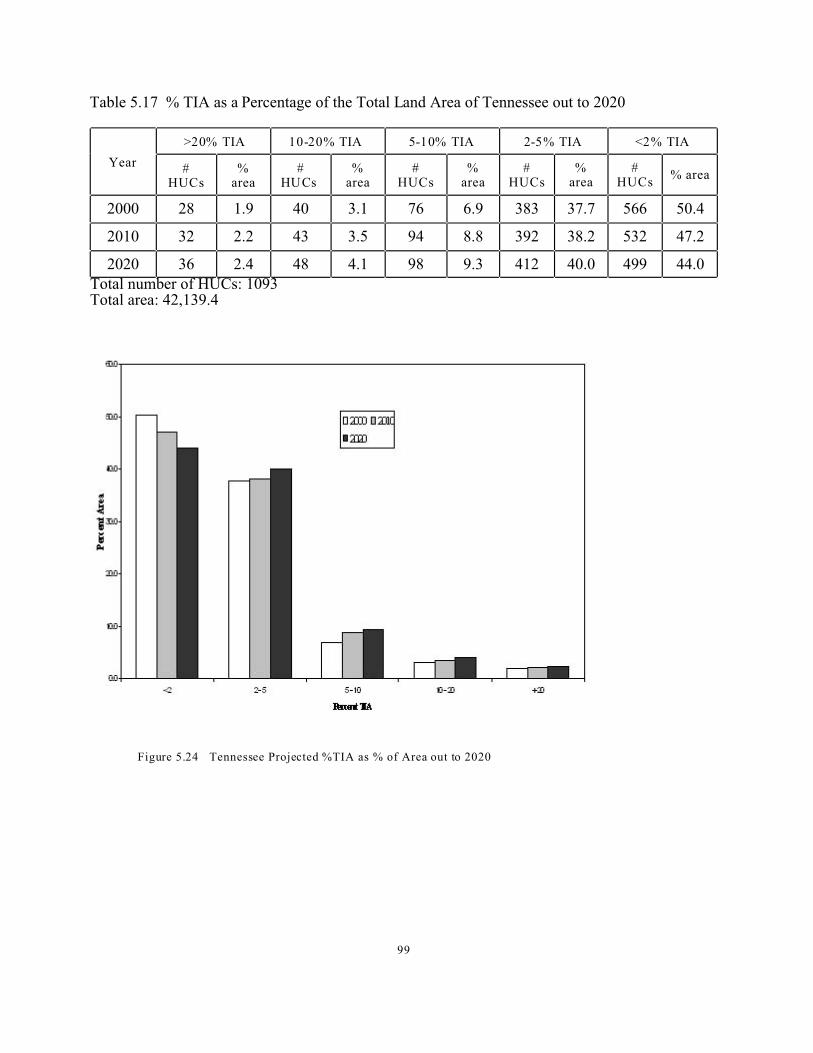
Table 5.17 % TIA as a Percentage of the Total Land Area of Tennessee out to 2020

Year

>20% TIA 10-20% TIA 5-10% TIA 2-5% TIA <2% TIA

# HUCs

% area

# HU Cs

% area

# HUCs

% area

# HUCs

% area

# HUCs

% area

2000 28 1.9 40 3.1 76 6.9 383 37.7 566 50.4

2010 32 2.2 43 3.5 94 8.8 392 38.2 532 47.2

2020 36 2.4 48 4.1 98 9.3 412 40.0 499 44.0 Total number of HUCs: 1093 Total area: 42,139.4

Figure 5.24 Tennessee Projected %TIA as % of Area out to 2020

99

Table 5.18 Total River Miles in Tennessee per TIA category

Year

>20% TIA 10-20% TIA 5-10% TIA 2-5% TIA <2% TIA

# HUCs

river miles

# HUCs

river miles

# HUCs

river miles

# HUCs

river miles

# HUCs

river miles

2000 28 994 40 1740 76 4151 383 24025 566 33072

2010 32 1143 43 1995 94 5392 392 24280 532 31173

2020 36 1226 48 2384 98 5628 412 25492 499 29251 Total number of HUCs: 1093 Total river miles: 63,981

Figure 5.25 Total River Miles in Tennessee by %TIA Category out to 2020

100

5.4 Using the Impervious Cover Projections

As discussed in Section 5.1, population projections for small (12 or 14 digit HUC scale)and rapidly growing places will be quite large. The population projections alone in HUCs in high growth areas can have errors in the 30 to 50% range for a 20 year time horizon. Impervious covercalculations for future periods will add additional errors in addition to the very substantial errors associated with small scale population projections. A good assessment of impervious cover projections can only come as a retrospective analysis similar to what has been done at multiple scales for population projections discussed in Section 5.1.

The projections of impervious cover are not meant to be used as definitive forecasts of the future state of a specific watershed, but rather as a plausible scenario to identify where to look for potential impairments and begin timely prevention efforts. These projections can give state and local planners and resource managers a reasonable assessment of the magnitude of the problems the states need to prepare for in the upcoming decades and can be used to guide monitoring to identify problems as they begin to surface. Stream remediation is very expensive. The North Carolina Ecosystem Enhancement Program stream reported costs for restoration/rehabilitation ofurban streams in 2004 to be $201.00 per foot of stream length (Jurek 2004). Well-timed and targeted prevention and management actions can avoid the need for at least some of these very expensive remediation expenditures in the future. Spatial tools, including the impervious coverprojections for the Southeastern states presented in this section, can aid in targeting these prevention and management activities.

101

6. Conclusions and Recommendations

Complete identification and eventual prevention of urban water quality problems pose significant monitoring and water quality management challenges. The purpose of the methodsand analyses discussed in this report was to provide tools to assist decision makers in meetingthese challenges. The Multiple Data Source (MDS) wide area impervious estimation andprojection techniques can assist in meeting these challenges by providing: 1) cheap estimates ofimpervious cover at the watershed and sub-watershed scales; 2) a region-wide approach to screening for waters likely impaired or threatened by urban storm water; and 3) projections of change in imperviousness over time.

The point sampling approach to aerial photo interpretation of imperviousness supplied an essential, cost-effective, independent assessment for both the MDS and the NLCD only estimation techniques and identified the appropriate uses for these two approaches. The use of the NLCD data with the ATtILA tool identifies most watersheds that are likely suffering severe impairment from urbanization and allows a very rapid assessment. Unfortunately, this tool is not as robust in identifying watersheds whose condition may be in a borderline category and vulnerable to impairment in the near future. The MDS technique provides a more reliable method for identifying watersheds impaired by urbanization compared to the use of land-use/land-cover alone, especially for watersheds in the 5 to 10% impervious range where prevention of storm water problems is critical.

The region-wide MDS impervious area estimates provide a screening tool for designing water quality monitoring programs by identifying areas for priority monitoring for urban and urbanizing watersheds. State monitoring programs have limited resources and thus cannot sample everywhere. This landscape screening process provides workable, defensible methods to:extrapolate condition estimates to waters lacking in-stream data; identify suspected problem areas (likely impaired waters); and efficiently target additional monitoring to confirm problems.

The current (year 2000) impervious area estimates of this study identify specific watersheds/HUC’s where existing adverse impacts due to impervious surfaces are likely (the 10 to 20% and >20% impervious classes). Some urban streams in these watersheds are listed as impaired through Section 303(d) of the Clean Water Act and are subject to TMDL development. Many potentially degraded waters are not yet listed, however, primarily due to a lack of systematic monitoring approaches to identify urban water quality problems. Using the results presented in this study, streams in watersheds/HUCs with imperviousness exceeding 10% that are not already listed under the 303(d) impaired waters listing process for sediment and biological integrity impairment should be prioritized for monitoring to ascertain if they are in fact impaired.

Prevention is critical. Stream channels de-stablized by excessive urban storm water runoff from impervious surfaces continue to erode for many decades (or longer) (Hammer 1972), have little potential to recover naturally and can be restored only with great difficulty and expense (Rosgen 1994). Successful rehabilitation and restoration of streams in urbanized watersheds will require complex, holistic approaches and should follow the sequence of: 1) hydrology, 2) channel and habitat, 3) riparian zones, and 4) aquatic biological communities, recommended bythe National Research Council (National Research Council 1992, and Brosnan, et al. 1999). The future impervious area projections of this study highlight the high growth areas of the Southeast, and the specific watersheds/HUC’s where this growth will be most likely to occur. These are the very areas where effective storm water management and prevention of urban storm water impacts are likely to be most cost effective. These same areas should be carefully considered to receive increased attention for storm water education for local leaders and the public, and to institute state-of-the-art storm water management practices. HUCs currently within the 5 to 10%

102

imperviousness range and projected to experience growth in the next decade need to be the highest priority focus of educational efforts and proactive storm water management actions to prevent water quality degradation.

A three to four fold increase of urban area in the Southeast over the next 40 years need not result in the widespread destruction of our streams, a resource vital to every community’s quality of life. If we focus now on the importance of imperviousness to future stream health, we can avoid totally unnecessary storm water degradation of streams, and put those waters already impacted back on the road to recovery.

Additional research will be needed to describe and explain differences in sensitivity to impervious cover and hydrologic storm water stress in different areas. A number of geographic frameworks should be tested to evaluate the variation in response to hydrologic stress from impervious areas including: ecoregions and subecoregions (McMahon, et al. 2001); hydrologic landscapes (Winter 2001); and average hydrologic response (Woodruff and Hewlett 1970). Relationships to in-stream response need to be refined for the Piedmont ecological region and developed using existing and new data for other areas of the Southeast. This might be doneregion by region (such as the Blue Ridge, Piedmont, and upper/lower coastal plains in North Carolina) using appropriate biological data sets encompassing the full gradient of imperviousness, or by using more generalized techniques such as multi-variate analyses incorporating critical physical factors likely to drive stream channel and sediment processes (and thus influence habitatand biological responses) such as relief, slope, soil properties (erodability in particular) and riparian vegetation. A potential advantage of the latter approach is that resulting response models might be applicable to much broader regions. The USGS’s series of “urban gradient” studies, which are gathering both landscape and in-stream data for a variety of urban areas around the nation, as well as existing state biological data networks, should provide useful data for building reliable empirical response models. Such efforts could provide valuable information to help understand variations in response to imperviousness and other urban stresses. Since some impervious areas are not directly connected to streams and other waters, work is also needed to incorporate cost-effective estimates of effective impervious area into storm water planning (Sutherland 1995 and Alley and Veenhuis 1983).

Tools to estimate impervious area and in-stream response attack just one of many stresses associated with urban expansion (Karr 1999). Practical screening tools are also needed fornutrient and upland sediment loading (Jones, et al. 2001, and Wickham, et al. 2002), bacterialcontamination (Mallin, et al. 2000) and for pesticide/herbicide contamination.

103

References

Allan, J.D. 1995. Steam ecology. Chapman & Hall, London, England.

Allan, J.D. 2004. Landscapes and Riverscapes: The Influence of Land Use on Stream Ecosystems. Annual Review of Ecology, Evolution, and Systematics. 35:257-284.

Allen, J. and K. Lu. 2003. Modeling and prediction of Future Urban Growth in the Charleston Region of South Carolina: a GIS-based Integrated Approach. Conservation Ecology. 8(2):2.[online] URL: http://www.consecol.org/vol8/iss2/art2

Alley, W.A. and J.E. Veenhuis. 1983. Effective impervious area in urban runoff modeling. Journal of Hydrological Engineering. ASCE. 109(2):313-319.

Brosnan, T., B.K. Ferguson, R. Iosco, G. Moll, T. Schueler, R. Sotir, and R. Watson. 1999. Mitigation of urban runoff impacts on Atlanta streams. Proceedings of the 1999 Georgia Water Resources Conference. March 30-31, 1999. Kathryn J. Hatcher, ed. Institute of Ecology, University of Georgia. Athens, GA. pp. 158-161.

Anderson, J.F., E.E. Hardy, J.T. Roach, and R.E. Witmer. 1976. A Land Use and Land Cover Classification System for Use with Remote Sensor Data. U.S. Department of the Interior, Geological Survey. Professional Paper 28.

Arnold, C.L., Jr. and C.J. Gibbons. 1996. Impervious Surface Coverage: The Emergence of a Key Environmental Indicator. Journal of the American Planning Association 62(2): 243-258.

Bergstedt, L.C. and E.P. Bergersen. 1997. Health and movements of fish in response to sediment sluicing in the Wind River, Wyoming. Canadian Journal of Fisheries and Aquatic Sciences 54: 312-319.

Bird, S.L., S.W. Alberty and L.R. Exum. 2000. Generating High Quality Impervious Cover Data. Journal of Quality Assurance. 8:91-103.

Booth, D.B. and C.R. Jackson. 1994. Urbanization of aquatic systems - degradation thresholds and the limits of mitigation. Effects of Human-Induced Changes on Hydrologic Systems ­American Water Resources Association. June 1994. pp. 425-434.

Borgman, L.E. and W.F. Quimby. 1988. Sampling for Tests of Hypothesis When Data Are Correlated in Space and Time. In Principles of Environmental Sampling, edited by L. H. Keith. Salem, MA: American Chemical Society.

Boward, D., P. Kazyak, S. Stranko, M. Hurd and A. Prochaska. 1999. From the mountains to the sea: The state of Maryland’s freshwater streams. U.S. Environmental Protection Agency. Office of Research and Development. EPA/903/R-99/023. 54pp.

Brosnan, T., Ferguson, B.K., Iosco, R., Moll, G., Schueler, T., Sotir, R., and Watson, R. 1999. Mitigation of urban runoff impacts on Atlanta streams. Proceedings of the 1999 Georgia Water Resources Conference. March 30-31, 1999. Kathryn J. Hatcher, ed. Institute of Ecology, University of Georgia. Athens, GA. pp. 158-161.

104

Brown, M.T. and M.B. Vivas. 2004. Landscape Development Intensity Index. Environmental Monitoring and Assessment. In Press.

Campbell, P. 1997. Current Population Reports, Population Projections: States, 1995-2025. U.S. Census Bureau, U.S. Department of Commerce, Economics and Statistics Administration. P25­1131.

Campbell, P.R. 2002. Evaluating forecast error in state population projections using Census 2000 counts. Population Division Working Paper Series No. 57. U.S. Bureau of the Census. 14pp.

Caraco, D., R. Claytor, P. Hinkel, H.Y. Kwon, T. Schueler, C. Swann, S. Vysotsky and J. Zielinske. 1998. Rapid Watershed Planning Handbook: A comprehensive guide for managing urbanizing watersheds. Center for Watershed Protection. Ellicott City, Maryland.

Center for Watershed Protection. 2003. Impacts of Impervious Cover on Aquatic Systems. Watershed Protection Research Monograph No. 1. Ellicott City, MD.

Chaloud, D.J., C.M. Edmonds and D.T. Heggem. 2001. Savannah River Basin landscape analysis. U.S. Environmental Protection Agency. Office of Research and Development. Washington, DC. EPA/600/R-01/069.

Corbett, C.W., M. Wahl, D.E. Porter, D. Edwards and C. Moise. 1997. Nonpoint source runoffmodeling: A comparison of a forested watershed and an urban watershed on the South Carolina coast. Journal of Experimental Marine Biology and Ecology. 213(1):133-149

Dartiguenave, C.M.and D.R. Maidment 1997. Water quality master planning for Austin. Center for Research in Water Resources (CRWR). University of Texas at Austin, Bureau of Engineering Research, Austin, Texas. CRWR Online Report 97-6.http://www.crwr.utexas.edu/reports/pdf/1997/rpt97-6.pdf

Ebert, D.W. and T.G. Wade. 2000. Analytical Tools Interface for Landscape Assessments (ATtILA) User Guide: Version 2.0. Office of Research and Development. U.S. Environmental Protection Agency. Las Vegas, NV. 23pp.

Environmental Systems Research Institute (ESRI). 1996. Using ArcView GIS. ESRI, Inc., Redlands, CA.

Florida Office of Economic and Demographic Research, “Demographic Information forMembers and Staff”, accessed February 2004, www.state.fl.us/edr/.

Gaff, W.L. 2001. Damage control: Restoring the physical integrity of America’s rivers. Annals of the Association of American Geographers. 91:1, 1-27.

Georgia Office of Planning & Budget (OPB). June 2002. Policy, Planning and Technical Support, State of Georgia OPB, Atlanta, Georgia.

Gillies, R.R., J.B. Box, J. Symanzik, and E.J. Rodemaker. 2003. Effects of urbanization on the aquatic fauna of the Line Creek watershed, Atlanta: a satellite perspective. Remote Sensing ofEnvironment. 86:3. 411-422.

105

Goetz, S.J., R.K. Wright, A.J. Smith, E. Zinecker and E. Schaub. 2003. IKONOS imagery for resource management: Tree cover, impervious surfaces, and riparian buffer analyses in the mid-Atlantic region. Remote Sensing of Environment. 88:1-2. 195-208.

Graham, P. H., L. S. Costello and H.J. Mallon. 1974. Estimation of Imperviousness and Specific Curb Length for Forecasting Storm water Quality and Quantity. Journal Water Pollution Control Federation. 46(4):717-725.

Griffith, G.E., J.M. Omernik, J.A. Comstock, M.P. Schafale, W.H. McNab, D.R. Lenat, T.F. MacPherson, J.B. Glover and V.B. Shelburne. 2002. Ecoregions of North Carolina and South Carolina (color poster with map, descriptive text, summary tables and photographs). Reston, Virginia. U.S. Geological Survey (map scale 1:1,500,000).

Griffith, J.A., S.V. Stehman and T.R. Loveland. 2003. Landscape Trends in Mid-Atlantic and Southeastern United States Ecoregions. Environmental Management. 32(5):572-588.

Griffith, J.A., E.A. Martinko, J.L. Whistler and K.P. Price. 2002. Interrelationships among landscapes, NDVI, and stream water quality in the U.S. Central Plains. Ecological Applications.12(6): 1702-1718.

Groffman, P.M., J.J. Bain, L.E. Band, K.T. Belt, G.S. Brush, J.M. Grove, R.V. Pouyat, I.C. Yesilonis and W.C. Zipperer. 2003. Down by the riverside: urban riparian ecology. Frontiers in Ecology and the Environment. 1(6): 315-321.

GVS&DD (Greater Vancouver Sewerage and Drainage District). 1999. Assessment of current and future GVS&DD area watershed and catchment conditions. url: < http://www.gvrd.bc.ca/sewerage/stormwater_reports_1997_2002/assessment/main_rpt/assessmen t_watersheds_catchments.pdf > last accessed March 7, 2005.

Hammer, T.B. 1972. Stream channel enlargement due to urbanization. Water Resources Research. 8:1530-1540.

Harper, G., Coleman, C., and Devine, J. 2003. Evaluation of 2000 subcounty population estimates. Population Division Working Paper Series No. 70. U.S. Bureau of the Census. 24pp.

Harrison, J., P. Hayward and B. Walker. 2001. Lullwater Fork Improvement Project (Atlanta, GA USA): Integrating Innovative Urban Watershed, Hydrology and Planning Approaches with “the Usual” Monitoring. Proceedings of the 6th National Volunteer Monitoring Conference:Moving Into the Mainstream. April 26-29, 2000. Austin, TX. US Environmental Protection Agency. EPA 841-R-01-001. pp. 129-134.

Harrison, J.E. 1998. Key water quality monitoring questions: Designing monitoring and assessment systems to meet multiple objectives. Proceedings of the National Water Quality Monitoring Council National Conference. Reno, NV. pp. III-175-187.

Hicks, R.W.B. and S. D. Woods. 2000. Pollutant Load, Population Growth and Land Use. Progress: Water Environment Research Foundation. 11: p. 10 url: <http://www.werf.org/press/fall00/00flplut.cfm > last accessed March 10, 2005.

106

Holland, F., D.M. Sanger, C.P. Gawle, S.B. Lerberg, M.S. Santiago, G.H.M. Riekerk, L.E. Zimmerman and G.I. Scott. 2004. Linkages between tidal creek ecosystems and the landscape and demographic attributes of their watersheds. Journal of Experimental Marine Biology and Ecology. 298(2):151-178.

Hulse, D. and R. Ribe. 2000. Land Conversion and the Production of Wealth. Ecological Applications. 10(3):679-681.

Inman, E.J. 2000. Lagtime relations for urban streams in Georgia. U.S. Geological Survey. Water Resources Investigations Report 00-4049. Atlanta, GA. 12 pp.

Inman, E.J. 1995. Flood-frequency relations for urban streams in Georgia - 1994 update. U.S. Geological Survey. Water Resources Investigations Report 95-4017. Atlanta, GA. 27 pp.

Jennings, D.B. and S.T. Jarnagin. 2002. Changes in anthropogenic impervious surfaces, precipitation and daily streamflow discharge: a historical perspective in a mid-atlantic subwatershed. Landscape Ecology. 17(5):471-489.

Jennings, David B., S.T. Jarnagin and D.W. Ebert. 2004. A Modeling Approach for Estimating Watershed Impervious Surface Area from National Land Cover Data 92. Photogrammetric Engineering & Remote Sensing. 70(11): 1295-1307.

Ji, M. and J.R. Jensen. 1999. Effectiveness of subpixel analysis in detecting and quantifying urban imperviousness from Landsat Thematic Mapper Imagery. Geocarto International. 14(4):33-41.

Jones, K.B., A.C. Neale, M.S. Nash, R.D. Van Remortel, J.D. Wickham, K.H. Riitters and R.V. O’Neill. 2001. Predicting nutrient and sediment loadings to streams from landscape metrics: A multiple watershed study from the United States Mid-Atlantic region. Landscape Ecology. 16: 310-312.

Kaiser Statehealthfacts.org, Kaiser Family Foundation, accessed December 2004, http://www.statehealthfacts.kff.org/cgi-bin/healthfacts.cgi?

Karr, J.R. 1999. Urbanization and stream biology: The dangers of basing permit decisions on total impervious area. Northwest Biological Assessment Workgroup. 10th Annual Meeting. Port Angeles, Washington. November 3-5,1999.

Kienegger, Erwin H. 1992. Assessment of a Wastewater Service Charge by Integrating Aerial Photography and GIS. Photogrammetric Engineering & Remote Sensing. 58(11):1601-1606.

Lee, K.H. 1987. Determining Impervious Area for Storm Water Assessment. Paper read at American Society of Photogrammetry and Remote Sensing/American Congress on Surveying and Mapping Annual Convention, 1987, at Baltimore, Maryland.

Mallin, M.A., K.E. Williams, E.C. Esham and R.P. Lowe. 2000. Effect of human developmenton bacteriological water quality in coastal watersheds. Ecological Applications. 10(4): 1047-1058.

Maryland Office of Planning. 1999. MdProperty View, Maryland Office of Planning, Planning Data Services Division, Baltimore, MD 21201.

107

May, C.W., R.R. Horner, J.R. Karr, B.W. Mar and E.B. Welch. 1997. Effects of Urbanization on Small Streams in the Puget Sound Lowland Ecoregion. Watershed Protection Techniques. 2: 483-493.

McMahon, G., S.M. Gregonis, S.W. Waltman, J.M. Omernik, T.D. Thorson, J.A. Freeouf, A.H.Rorick and J.E. Keys. 2001. Developing a spatial framework of common ecological regions for the conterminous United States. Environmental Management. 28(3):293-316.

Miltner, R.J., D. White and C. Yoder. 2004. The biotic integrity of streams in urban and suburbanizing landscapes. Landscape and Urban Planning. 69:87-100.

Mississippi Institutions of Higher Learning. March 2002. “Mississippi Population Projections”,Center for Policy Research and Planning, Jackson, Mississippi.

Mitchell, J.G. and S. Leen. 2001. Urban Sprawl. National Geographic. 200:1, July 2001. 48­73. http://magma.nationalgeographic.com/ngm/data/2001/07/01/html/ft_20010701.3.html#

National Research Council. 1992. Restoration of Aquatic Ecosystems: Science, Technology and Public Policy. National Academy Press. Washington, DC. 576pp.

Nash, M.S. and D.J. Chaloud. 2002. Multivariate Analyses (Canonical Correlation and Partial Least Square (PLS)) to Model and Assess the Association of Landscape Metrics to Surface Water Chemical and Biological Properties Using Savannah River Basin Data. U.S. Environmental Protection Agency. Office of Research and Development. Washington, DC. EPA/600/R-02/091.

Newcombe, C.P. and D.D. MacDonald. 1991. Effects of suspended sediments on aquatic ecosystems. North American Journal of Fisheries Management. 11: 72-82.

Nichols, D.B., B.K. Ferguson, S. Seinberg and M.A.A. Akers. 1999. Development ordinances to protect streams. Proceedings of the 1999 Georgia Water Resources Conference. March 30-31, 1999. Kathryn J. Hatcher, ed. Institute of Ecology, University of Georgia. Athens, GA. pp. 151­154.

North Carolina Department of Environment and Natural Resources. 2003. Standard operatingprocedures for benthic macroinvertebrates. Biological Assessment Unit. Raleigh, NC. 21pp.

North Carolina Department of the Environment and Natural Resources (NCDENR). 2002. North Carolina Division of Water Quality, Water Supply Watershed Protection, “Streamlines”, Volume 6, Issue 3, http://h2o.enr.state.nc.us/wswp/SL/v6i3.pdf

North Carolina Office of State Budget and Management. June 2003. North Carolina State Data Center, Raleigh, North Carolina.

Office of Management and Budget (OMB). December 27, 2000 Federal Register Notice, Standards for Defining Metropolitan and Micropolitan Statistical Areas, Vol. 65, No. 249, accessed 2004 at http://www.census.gov/population/www/estimates/00-32997.pdf

Omernik, J. 2003. The Misuse of Hydrologic Unit Maps for Extrapolation, Reporting and Ecosystem Management. Journal of the American Water Resources Association. 39(3): 563-573.

108

Paul, M.J. and J. Meyer. 2001. Streams in the urban landscape. Annual Review of Ecology and Systematics. 32:333-65.

Poff, N.L, J.D. Allan, M.B. Bain, J.R. Karr, K.L. Prestegaard, B.D. Richter, R.E. Sparks and J.C. Stromberg. 1997. The natural flow regime: A paradigm for river conservation and restoration. BioScience. 47(11):769-784.

Potter, K.M., F.Q. Cubbage and R.H. Schaberg. 2005. Multiple-scale landscape predictors ofbenthic macroinvertebrate community structure in North Carolina. Landscape and Urban Planning. 71:77-90.

Price, M., M. Scorbee and T. Sawyer. “Kentucky Migration: Consequences for State Population & Labor Force,” 2004. University of Louisville, Urban Studies Institute.

Reeves, G.H., L.E. Benda, K.M. Burnett, P.A. Bisson, and J.R. Sedell. 1995. A disturbance-based ecosystem approach to maintaining and restoring freshwater habitats of evolutionary significantunits of anadromous salmonids in the Pacific Northwest. American Fisheries Society Symposium 17: 334-349.

Richter, B.D., J.V. Baumgartner, J. Powell and D.P. Braun. 1996. A method for assessing hydrologic alteration within ecosystems. Conservation Biology. 10:1163-1174.

Richter, B.D., D.P. Braun, M.A. Mendelson and L.L. Master. 1997. Threats to imperiledfreshwater fauna. Conservation Biology. 11:1081-1093.

Rosgen, David L. 1994. A classification of natural rivers. Catena. 22:169-199.

Schueler, T. 1994. The Importance of Imperviousness. Watershed Protection Techniques. 1: 100-111.

Seaber, P.R., F.P. Kapinos and G.L. Knapp. 1987. Hydrologic Unit Maps: U.S. Geological Survey Water Supply Paper 2294, 63 p.

Sleavin, W.J., S. Prisloe, L. Giannotti, and D.L. Civco. 2000. Measuring impervious surfaces for non-point source pollution modeling, 2000 American Society for Photogrammetry and Remote Sensing (ASPRS) Annual Convention, Washington, DC.

Slonecker, E.T., D.B. Jennings and D. Garofalo. 2001. Remote Sensing of Impervious Surfaces: A Review. Remote Sensing Reviews. 20:227-255.

Smith, S.K. 1987. Tests of forecast accuracy and bias for county population projections. Journal of the American Statistical Association. 82(400):991-1013.

Smith, S.K. and J.M. Nogle. “Florida Population Studies: Population Projections by Age, Sexand Race for Florida and its Counties, 2002-2025.” July 2003. Vol 36, No. 3, Bulletin 136.

Smith, S.K. and Shahidullah, M. 1995. An evaluation of population projection errors for census tracts. Journal of the American Statistical Association. 90(429):64-71.

Smith, S.K. and Sincich, T. 1992. Evaluating the forecast accuracy and bias of alternative population projections for states. International Journal of Forecasting. 8:495-508.

109

Smith, S.K. and Sincich, T. 1990. The relationship between the length of the base period and population forecast errors. Journal of the American Statistical Association. 85(410):367-375.

Snyder, C.D., J.A. Young, R. Villella and D.P. Lemarie. 2003. Influences of upland and riparian land use patterns on stream biotic integrity. Landscape Ecology. 18:647-664.

South Carolina State Budget & Control Board. October 2002. Office of Research & Statistics, Health & Demographics Division, Columbia, South Carolina.

Stankowski, S.J. 1972. Population Density as an Indirect Indicator of Urban and Suburban Land-Surface Modifications, U.S. Geological Survey: B219-B224.

Stone, B., Jr. 2004. Paving over paradise: How land use regulations promote residential imperviousness. Landscape and Urban Planning. In Press.

Sutherland, R.C. 1995. Methodology for estimating the effective impervious area of urban watersheds. Technical Note 58. Watershed Protection Techniques. 2(1)282-284.

Trimble, S.W. 1997. Contribution of stream channel erosion to sediment yield from an urbanizing watershed. Science. 278:1442-1444.

University of Alabama. August 2001. Center for Business and Economic Research, Culverhouse College of Commerce, Tuscaloosa, Alabama.

University of Florida. July 2003. Bureau of Economic and Business Research, WarringtonCollege of Business Administration, Gainesville, Florida.

University of Louisville. July 2003. Kentucky State Data Center, Urban Studies Institute, Louisville, Kentucky.

University of Tennessee. March 1999. Center for Business and Economic Research, College of Business Administration, Knoxville, Tennessee.

U.S. Census Bureau. 2001. Census 2000 Redistricting Data (P.L. 94-171) Summary File and 1990 Census. Census 2000 PHC-T-2. Ranking Tables for States: 1990 and 2000, Table 1: States Ranked by Population 2000, internet release date April 2001.

U.S. Census Bureau. April 2001. Census 2000 Redistricting Data (P.L. 94-171) Summary File and 1990 Census. Census 2000 PHC-T-2. Ranking Tables for States: 1990 and 2000, Table 2: States Ranked by Numeric Population Change: 1990 to 2000, internet release date April 2001.

U.S. Census Bureau. State and County QuickFacts, 2004. http://quickfacts.census.gov/qfd/states/01000.html

U.S. Census Bureau. Metropolitan and Micropolitan Statistical Area Definitions, 2004.http://www.census.gov/population/www/estimates/metroarea.html or U.S. Census Bureau, Metropolitan Area Page Size Maps, 2004,http://www.census.gov/geo/www/mapGallery/mapage.html

110

U.S. Department of Agriculture. 1997. AREI Updates on Agricultural Resources and Environmental Indicators, Economic Research Service, Natural Resources and Environment Division, Washington, DC, Number 3, June 1997, 4 pages.http://ers.usda.gov/publications/arei/97upd/upd97-3.pdf

U.S. Department of Agriculture. 2003. “Briefing Room: Land Use, Value, and Management: Major Uses of Land”, Economic Research Service, Washington, DC, internet document updated 10/270/2003. http://ers.usda.gov/Briefing/LandUse/majorlandusechapter.htm

U.S. Department of Agriculture. 2000. Summary Report: 1997 National Resources Inventory (revised December 2000), Natural Resources Conservation Service, Washington, DC, andStatistical Laboratory, Iowa State University, Ames, Iowa, 89 pages. http://www.nrcs.usda.gov/technical/nri/1997/summary_report/

U.S. Department of Transportation. 2001. National Transportation Atlas Databases, National Highway Planning Network (NHPN)Version 3.0. Bureau of Transportation Statistics, Federal Highway Administration, Office of Intermodal and Statewide Programs (HEPS-20), Washington, DC.

USEPA. 2000a. BASINS Technical Note 6: Estimating Hydrology and Hydraulic Parameters for HSPF. U.S. Environmental Protection Agency, Office of Water, Washington, DC. EPA/823/R-00/012.

USEPA. 2000b. Better Assessment Sciences Integrating Point and Nonpoint Sources (BASINS). U.S. Environmental Protection Agency, Office of Water, Office of Science and Technology, Washington, DC.

USEPA. 1994. The Quality of Our Nation's Water: 1992. U.S. Environmental Protection Agency, Office of Water, Washington, DC. EPA/841/F-94/002.

Vogelmann, J.E., T. Sohl and S.M. Howard. 1998a. “Regional Characterization of Land Cover Using Multiple Sources of Data.” Photogrammetric Engineering & Remote Sensing. 64(1): 45­57.

Vogelmann, J.E., T. Sohl and S.M. Howard. 1998b. Regional Land Cover Characteristics using Landsat Thematic Mapper Data and Ancillary Data Sources. Environmental Monitoring andAssessment. 51:415-428.

Vogelmann, J.E., S.M. Howard, L. Yang, C.R. Larson, B.K. Wylie and N. Van Driel. 2001. Completion of the 1990s National Land Cover Data Set for the Conterminous United States from Landsat Thematic Mapper Data and Ancillary Data Sources. Photogrammetric Engineering and Remote Sensing. 67:650-652.

Wear, David N. and J.G. Greis. 2002. Southern Forest Resource Assessment Final Report. Southern Research Station, USDA Forest Service, and Southern Region, USDA Forest Service. http://www.srs.fs.usda.gov/sustain

Wickham, J.D., R.V. O’Neill, K.H. Riitters, E.R. Smith, T.G. Wade and K.B. Jones. 2002. Geographic targeting of increases in nutrient export due to future urbanization. Ecological Applications. 12(1):93-106.

111

Wilcove, D.S., D. Rothstein, J. Dubow, A. Phillips and E. Losos. 1998. Quantifying threats to imperiled species in the United States. BioScience. 48:607-615.

Williams, J.E., J.E. Johnson, D.A. Hendrickson, S. Contreras-Balderas, J.D. Williams, M. Navarro-Mendoza, D.E. McAllister and J.E. Deacon. 1989. Fishes of North America: endangered, threatened, or of species concern. Fisheries 14: 2-20.

Winter, T.C. 2001. The concept of hydrologic landscapes. Journal of the American Water Resources Association. 37(2):335-349.

Wolman, M.G. 1967. A cycle of sedimentation and erosion in urban river channels. Geografiska Annaler. 49A(2-4):385-395.

Woodruff, J.F. and J.D. Hewlett. 1970. Predicting and mapping the average hydrologic response for the Eastern United States. Water Resources Research. 6(5):1312-1326.

Yang, L., C. Huang, C. Homer, B. Wylie and M. Coan. 2003. An approach for mapping large-area impervious surfaces; synergistic use of Landsat 7 ETM+ and high spatial resolution imagery. Canadian Journal of Remote Sensing. 20(2):230-240.

Zandbergen, P., J. Houston and H. Schreier. 2000. Comparative Analysis of Methodologies for Measuring Watershed Imperviousness. Watershed Management 2000 Conference, Institute for Resources and Environment, University of British Columbia, Vancouver, British Columbia, Canada, July 2000.

112

Appendix

The following procedures were used to calculate the current and projected %TIA for the eight Southeastern United States: Alabama, Florida, Georgia, Kentucky, Mississippi, North Carolina, South Carolina and Tennessee. All the GIS work was done in Environmental Systems Research Institute, Inc.(ESRI)’s ArcView 3.2 and ArcInfo Workstion 9. The scripts in Section XIII are in the ArcView scripting language Avenue. Source data used in these processing steps include the following and are referred to by data type number (1-6) in the stepwise procedures.

1. NLCD 92 – 21 category land cover classification with 30 m spatial resolution raster (gridded) coverage (http://edc.usgs.gov/products/landcover/nlcd.html). Data was provided on CD by USEPA Region 4 for the eight Southeastern states from regional data archives.

2. National Transportation Atlas (NTA) available on CD from U.S. Department of Transportation (USDOT (2001) as a shapefile. Class 1 (interstates and major highways) roads for the eight Southeastern states were saved as a shapefile for use in analysis.

3. U.S. Bureau of Census 1990 and 2000 block level population and population density data. Block level data as a shapefile was provided by USEPA Region 4 from regional data archives for the eight Southeastern states.

4. U.S. Bureau of Census 2000 block level vacant housing data. Data was downloaded from U.S. Bureau of Census website (www.census.gov) and processed as described in Section Vbelow.

5. 12 or 14 digit HUC shapes files obtained from individual Southeastern states 6. County level population projections obtained from individual Southeastern states.

A state scale version for each of these data sets was developed and stored in state specific directories. The following procedures were used to calculate values for each of the eight individual states.

I. To calculate road area:Step 1: remove road arcs that run through commercial industrial and mining cells to preventdouble-accounting:

A. To obtain only the high intensity commercial grid cells (value=23) from data set 1, from the grid prompt in:GRID: outgrid = select(mrlc grid, ‘value = 23')

B. Convert the value23 grid to a polygon coverage by:ARC: gridpoly value23 value23_poly

C. Convert road shapefile (data set 2) to a coverage using the shapearc command in ARC. D. After setting up the ArcEdit: environment, ensure that the following two commands execute:

AE: nodesnap offAE: intersectarcs all

then “get” the poly arcs into the road coverage to make intersections at all polygons. Save and then select all arcs with lanes = 0 and delete. E. Convert the roads coverage back to a shapefile (newroadshape). F. In ArcView, use the select by theme option and select the road arcs in newroadshape

that are completely within the value = 23 polygons. Delete the selected arcs. G. Repeat steps A, B, C, and F to remove roads in grid cells classified as mining value =

32. Replace the number 23 with 32 in each of these steps.

Step 2: calculate road area: A. Select the 2-lane arcs (Lanes = 2) from newroadshape and create a new shapefile from

the selected two lane arcs.

113

B. Select-by-theme the huc polygons that are intersected by the 2-lane road arcs. Reverse the selection to select huc polygons that do not contain road arcs and calculate the 2-lane area to -9999. Then run the rd_clip.ave script.

C. Repeat steps A & B using 4-lane roads. D. The rd_clip.ave script will clip the road arcs with the huc polygon and calculate the

new road arc lengths in meters. The road lengths are then converted to road area in square miles using the following formula:

road length x 3.2808 x 24 (or 48) x 0.00000003587006Where 3.2808 is the conversion constant for meters to feet and 24 is the assumed width, in feet, of a two-lane road (48 is the width, in feet, for a four-lane road) and 0.00000003587006 is the conversion constant for square feet to square miles.

E. The field total_rd_area is calculate by adding the 2-lane and 4-lane area fields. The null values (-9999) will be re-calculated to -1111 by the script and then selected and recalculated after script completion to 0 since they contain no highway segment.

II. To calculate industrial and mining area:1. Obtain the high intensity commercial grid cells from data type 1 in ArcInfo using

GRID; GRID: outgrid = select(<grid name>, ‘value = 23')

2. Then convert the outgrid into a polygon coverage:ARC: gridpoly outgrid value23_poly

3. Convert value23_poly to a shapefile. 4. In ArcView select the huc polygons (Data type 5) that completely contain the features

of value23_poly.shp5. Reverse the selection and calculate the selected records’ commercial area field to

- 9999 and run the fixed_loop.ave. The cell count will be calculated to the area field. Converted to square meters, then convert to sq. miles. The other records (-9999) will be re-calculateded to -1111 and should be re-calculated to 0 since they contain no commercial property.

6. For mining, repeat above steps using the value 32 instead of 23. 7. The areas in square miles are calculated to the fields indus_area (or comm_area) and

mining_area respectively.

III. Populations for the years 2000 and 1990 and state population projections: 1. The FIPs code was calculated for the block shapefile (data set 2) by adding a field

([FIPS]) as a string with a width of five and calculating it equal to the [Areakey] field.

2. A new field was added to the block shapefile called [orig_area] and the value was calculated (Shape.ReturnArea).

3. The block shapefile was exported as a geodatabase and then converted back to a shapefile.

4. The avenue script clip_blocks.ave was run, which clips the blocks by the HUCs (data type 2).

5. The clipped blocks are then merged back together using the GeoProcessing Wizard in ArcView.

6 A new field, [new_area] is added and calculated. A [factor] field is also added and is calculated by [new_area] / [orig_area].

7. A selection is run on records with a factor > 1.01 and those are deleted. These values are believe to exist because of problems within the original block shapefile due to manipulation by the original creators to account for changes between 1990 and

114

2000. Records that have a zero population for both 1990 and 2000 are also deleted as they will not play a factor in any population estimates.

8. New population fields are added for 1990 and 2000 to the block shapefile and are calculated by multiplying the original populations by the factor value to get thecorrected population for the split blocks (new_pop2000 and new_pop1990).

9. An excel table containing the Census 1990 & 2000 figures per county along with the state’s population estimates for any or all of the following years: 2010, 2015, 2020, 2025, and 2030 was joined by FIPS code field to the block shapefile.

10. Block population estimates are calculated in the block shapefile by: block_popX = new_pop2000 / County_pop2000 * County_popX,

where X = year estimated. 11. The block population estimates are summed and calculated to the HUCs by running

the calc_pop.ave script. Minor edits are made to the script for each year’s estimate.

IV. Population Density:1. All population values divided by square miles.

V. Vacant Housing Data:Step 1: import data from Census website (data type 4):

A. Download each state’s files (for example, Alabama’s data would be named al00037ufl.zip (data) and algeoufl.zip (geography)) from the Census Bureau’s FTP site and unzip each file.

B. Dowloaded the Summary File template file for MSAccess97 from the Census Bureau’s website. This file enables the import of the data and geographic files into Access because it contains the field names and structure for the data. This site also includes instructions for importing the files into MSAccess.

C. Change the *00037.ufl and *geo.ufl file extensions to .txt and follow the importprocedures into MSAccess (instructions located at Census website.)

D. Save each database as a .dbf. E. Import the .dbf files into ArcView.F. Perform a join on the <logrecno> fields contained in both the geo and data files. G. Export the joined table as a new .dbf file to permanently preserve join. H. Create <Areakey> field as a string and calculated to match <areakey> in Region 4

block data. Populate the records by calculating the new field as state+county+tract+block (concatenate the values). Join the two tables (censusdata + block data).

Step 2: Calculate number of homes per type of vacancy:A. Calculate the following, per HUC (data type 5): total housing units, occupied units,

vacant units, rental homes, homes for sale, rented or sold homes that are vacant, seasonal housing, migrant housing and homes vacant for other reasons. The calculations are completed using the calc_vcn.ave script.

B. Density for vacant housing is based on number of homes per square mile. Step 3: Calculate estimated population for vacant housing:

A. Calculate population equivalent using the vacant housing information and average household size by state (based on data from US Census Bureau website) for each HUC. Calculation was a weighted average based on owner-occupied and renter-occupied---Average population per household for North Carolina = 2.48798 Average population per household for Alabama = 2.49575 Average population per household for Florida = 2.4601 Average population per household for Georgia = 2.645

115

Average population per household for Kentucky = 2.46824Average population per household for Mississippi = 2.62845Average population per household for South Carolina = 2.52884Average population per household for Tennessee = 2.48572

Average person per household multiplied by number of vacant homes. The total vacant and seasonal population fields are based only on vacant and seasonal housing data. The total vacant and seasonal population density field are based on the vacant and seasonal populations + the 2000 population per square mile.

VII. %TIA values based on population: %TIA based on the Hicks (GVSS&DD) calculations use the following formula:

(94 x (1 - (2.7183 ^ (-0.00010938 x PopulationDensityValue)))) + 1

VIII. Extrapolated 1993 Population Value:The population value for 1993 was derived using:

1990 Population + (((2000 Population - 1990 Population) / 10) x 3)

IX. Projected high intensity commercial industrial (HICI) area: 1. HiciX = commercial area x PopulationX / 1993 Population

Where X = projected year2. Query: HiciX < commercial area; if yes, calc HiciX = commercial area 3. Add a temporary field, calculated as:

commercial area / 1993 population x 10,0004. Evaluate the temporary field to determine if any values are greater than 3. 5. If there are values greater than 3, add a temporary field, calculated as:

0.6 x (PopulationX - 1993 Population) / 10,0006. Use the value from Step 5 and add it to the commercial area to determine

HiciX for that record. 7. Reevaluate HiciX < commercial area and recalculate HiciX = commercial area if necessary.

X. Commercial Total Impervious Area: % Commercial TIA is calculated as:

(HiciX / total area HUC) x 0.90 x 100

XI. Percent Total Impervious Area: Percent TIA is calculated as:

% road area + % mining area + % Commercial TIA + Hicks calculation The field TIA2000_vct using the above formula with the Hicks value (Step VII) being calculated from the total vacant population density figure (from Section V, Step 3.)

XII. Projected Population with Vacant:1. Projected population for 2010, 2015, etc with projected vacant population added:

Year X projected HUC population * (1 + total vacant population / 2000 population)2. The density is then calculated by dividing by area in square miles.

116

XIII. Scripts:

• Script 1: Fixed_loop.ave

'loop_grd_clp.ave'Christine Perkins, CSC'this scrip loops through a polygon coverage, selects each polygon'using an index number,'clips the grid and returns the count value to be calculated into the'polygon attribute table.

theProject = av.GetProjecttheView = theProject.FindDoc("View1")PolyThm = theView.FindTheme("huc12_al.shp")GridThm = theView.FindTheme("mining_grid")GridThm.SetActive(true)PolyFTab = PolyThm.GetFTab

theField = PolyFTab.FindField("Index")theField2 = PolyFTab.FindField("mining_area")PolyFTab.SetEditable(true)theSel = PolyFTab.GetSelection

theValue = 0for each rec in PolyFTab

theValue = theValue + 1 QueryString = "[Index] =" + theValue.AsStringPolyFTab.Query(QueryString,theSel,#VTAB_SELTYPE_NEW)PolyFTab.UpdateSelectionnewVal = PolyFTab.ReturnValue(theField2,rec)

if (newVal < 0) thenPolyFTab.SetValueNumber(theField2,rec,-1111)else

theGrid=theView.GetActiveThemes.Get(0).GetGrid

'Get bounds of clipping area as a rectanglethePolyThmExtent = PolyThm.getselectedextentif (thePolyThmExtent .IsEmpty) then thePolyThmExtent =PolyThm.ReturnExtent end

'Get parameters for the new gridtheFtab = PolyThm.GetFTabtheProj = theView.GetProjectiontheCell = theGrid.GetCellSizetheExtent = theGrid.GetExtent

ae = theView.GetExtension(AnalysisEnvironment)ae.SetExtent(#ANALYSISENV_VALUE, thePolyThmExtent)ae.SetCellSize(#ANALYSISENV_VALUE, theCell)

' Activate the settings for the analysis envirnonment as returned' by the above 3 lines of code.ae.Activate

'the actual extraction occurs heretempGrid = Grid.MakeFromFtab(theFtab,theProj,nil,{theCell,theExtent})newGrid = (tempGrid.IsNull).Con (tempGrid, theGrid)

' rename data setaFN = av.GetProject.GetWorkDir.MakeTmp("mine", "")newGrid.Rename(aFN)

117

' check if output is okif (newGrid.HasError) then return NIL end

' create a theme gridThm = theme.make(newGrid.GetSrcName)

' set name of themegridThm.SetName("Huc" + theValue.AsString)

' add theme to the specifiedViewtheView.addTheme(gridThm)

' Resets the analysis environment to the maximum of inputs (i.e. thedefault)aRect = Nilae = theView.GetExtension(AnalysisEnvironment)ae.SetExtent(#ANALYSISENV_MAXOF, aRect)ae.SetCellSize(#ANALYSISENV_MAXOF, aRect)

gridThm.invalidate(true)

newerGrid = gridThm.GetGridnewVTab = newerGrid.GetVTabtheFieldest = newVTab.FindField("count")answer5 = newVTab.ReturnValue(theFieldest,0)

PolyFTab.SetValue(theField2,rec,answer5)theProject.saveendend

• Script 2: rd_clip.ave

'clip_themes.ave'Christine Perkins, May 2001'this script loops through a polygon-type shapefile, selects each'polygon,'clips and creates a road shapefile based on the poly boundaries,'calculates'the new road lengths, and plugs the length into the still-selected'polygon'uses the extensions Batch Clip and Clip Theme, available online.

'Basic setuptheProject = av.GetProjecttheView = theProject.FindDoc("View1")PolyThm = theView.FindTheme("Huc12_al.shp")PolyThm.SetActive(true)LineThm = theView.FindTheme("Four_lanes.shp")LineThm.SetActive(true)PolyFTab = PolyThm.GetFTabLineFTab = LineThm.GetFTab

'Finds necessary fields and sets up tablestheField = PolyFTab.FindField("Index")theField2 = PolyFTab.FindField("four_lane")PolyFTab.SetEditable(true)theSel = PolyFTab.GetSelection

'Starts the looptheValue = 0for each rec in PolyFTab

118

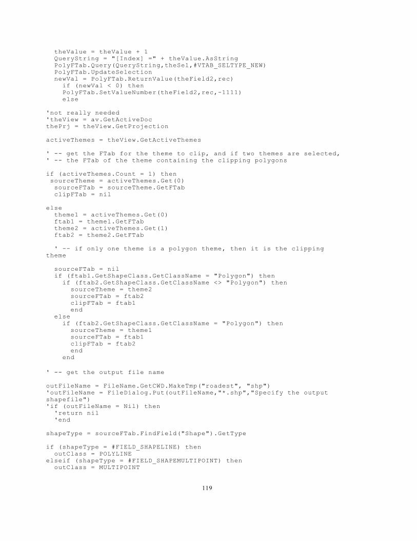
theValue = theValue + 1 QueryString = "[Index] =" + theValue.AsStringPolyFTab.Query(QueryString,theSel,#VTAB_SELTYPE_NEW)PolyFTab.UpdateSelectionnewVal = PolyFTab.ReturnValue(theField2,rec)

if (newVal < 0) thenPolyFTab.SetValueNumber(theField2,rec,-1111)else

'not really needed'theView = av.GetActiveDocthePrj = theView.GetProjection

activeThemes = theView.GetActiveThemes

' -- get the FTab for the theme to clip, and if two themes are selected,' -- the FTab of the theme containing the clipping polygons

if (activeThemes.Count = 1) thensourceTheme = activeThemes.Get(0)sourceFTab = sourceTheme.GetFTab

clipFTab = nil

else theme1 = activeThemes.Get(0)ftab1 = theme1.GetFTab

theme2 = activeThemes.Get(1)ftab2 = theme2.GetFTab

' -- if only one theme is a polygon theme, then it is the clippingtheme

sourceFTab = nil if (ftab1.GetShapeClass.GetClassName = "Polygon") then

if (ftab2.GetShapeClass.GetClassName <> "Polygon") thensourceTheme = theme2

sourceFTab = ftab2 clipFTab = ftab1end

else if (ftab2.GetShapeClass.GetClassName = "Polygon") then

sourceTheme = theme1 sourceFTab = ftab1 clipFTab = ftab2end

end

' -- get the output file name

outFileName = FileName.GetCWD.MakeTmp("roadest", "shp")'outFileName = FileDialog.Put(outFileName,"*.shp","Specify the outputshapefile")'if (outFileName = Nil) then

'return nil 'end

shapeType = sourceFTab.FindField("Shape").GetType

if (shapeType = #FIELD_SHAPELINE) thenoutClass = POLYLINE

elseif (shapeType = #FIELD_SHAPEMULTIPOINT) thenoutClass = MULTIPOINT

119

elseif (shapeType = #FIELD_SHAPEPOINT) thenoutClass = POINT

elseif (shapeType = #FIELD_SHAPEPOLY) thenoutClass = POLYGON

else 'MsgBox.Error("Invalid shape field type.",theTitle)' return nil

end

' -- check if shapes should be projected

'doProjection = false'if (thePrj <> nil) then

'doProjection = MsgBox.YesNo("Output shapes in projectedcoordinates?",theTitle,true)

'end

' -- create one large polygon from the input polygons

if (clipFTab <> nil) thenclipPoly = av.Run("View.ClipThemeUnionFTab",clipFTab)

else clipPoly = av.Run("View.ClipThemeUnionGraphics",theView)if (thePrj <> nil) then

clipPoly = clipPoly.ReturnUnprojected(thePrj)end

end

' -- select the features to be processed

oldSelection = sourceFTab.GetSelection.Cloneif (sourceFTab.GetSelection.Count = 0) then

sourceFTab.GetSelection.SetAll end

'if (clipOption = "inside") thensourceFTab.SelectByPolygon(clipPoly,#VTAB_SELTYPE_AND)processSelection = sourceFTab.GetSelection.Clone

sourceFTab.SetSelection(oldSelection)sourceFTab.UpdateSelection

' -- create the new shapefile

outFTab = FTab.MakeNew(outFileName, outClass)outFTab.SetEditable(true)

outFields = sourceFTab.GetFields.DeepCloneoutFields.Remove(0)outFTab.AddFields(outFields)outFields = outFTab.GetFieldsoutShapeField = outFTab.FindField("shape")

sourceFields = sourceFTab.GetFieldssourceShapeField = sourceFTab.FindField("shape")

' -- process the features

selCount = processSelection.Countc = 0av.ShowMsg("Clipping ...")av.SetStatus(0)

120

for each sRec in processSelections = sourceFTab.ReturnValue(sourceShapeField,sRec)'if (clipOption = "inside") then

if (s.IsContainedIn(clipPoly).Not) thens = s.ReturnIntersection(clipPoly)end

'if (doProjection) then' s = s.ReturnProjected(thePrj)' end

oRec = outFTab.AddRecord outFTab.SetValue(outShapeField,oRec,s)

for each i in 1..(sourceFields.Count - 1)v = sourceFTab.ReturnValue(sourceFields.Get(i),sRec)outFTab.SetValue(outFields.Get(i),oRec,v)end

c = c + 1 av.SetStatus((c / selCount) * 100)end

outFTab.SetEditable(false)av.ClearMsgav.ClearStatus

' -- display in a view if requested

viewList = List.Makefor each d in av.GetProject.GetDocs

if (d.Is(View)) thenviewList.Add(d)end

end

''add new theme newTheme = FTheme.Make(outFTab)theView.AddTheme(newTheme )theView.GetWin.Activate

end

''calculate length of road segmentsnewTab = newTheme.GetFTab

newTab.SetEditable(true)lengthField = Field.Make("Length3",#FIELD_DECIMAL,16,3)newTab.AddFields({lengthField})

'calc each segment's length and attribute the recordfor each rec in newTab theShape = newTab.ReturnValue(newTab.FindField("shape"),rec)x = theShape.ReturnLengthnewTab.SetValue(lengthField,rec,x)

end newTab.SetEditable(false)

'add lengths from new shapefile

total = 0theLength = newTab.FindField("Length3")

for each rec in newTab lengths = newTab.ReturnValue(theLength,rec)

121

total = total + lengthsend

'plug in length value into polygon recordPolyFTab.SetValue(theField2,rec,total)theProject.save

endend

• Script 3: Clip_blocks.ave

'TITLE: clip_blocks.ave'AUTHOR: Christine Perkins, CSC'PURPOSE: clips a block shapefile with a HUC shapefile and adds the'clipped blocks to the ArcView project

theProject = av.GetProjecttheView = theProject.FindDoc("View1")

SRCTheme = theView.FindTheme("Blocks_geo.shp")interTheme = theView.FindTheme("Arc_huc12.shp")interTheme.SetActive(true)interFTab = interTheme.GetFTabSRCFTab = SRCTheme.GetFTabinterFTab.SetEditable(true)theField = interFTab.FindField("Index")theSel = interFTab.GetSelection

theValue = 0for each rec in interFTab theValue = theValue + 1 QueryString = "[Index] =" + theValue.AsStringinterFTab.Query(QueryString,theSel,#VTAB_SELTYPE_NEW)interFTab.UpdateSelection

' Specify the output shapefile...outFName = FileName.GetCWD.MakeTmp("clip", "shp")

shapeType = SRCTheme.GetFTab.FindField("Shape").GetType

if (shapeType = #FIELD_SHAPELINE) thenoutClass = POLYLINE

elseif (shapeType = #FIELD_SHAPEMULTIPOINT) thenoutClass = MULTIPOINT

elseif (shapeType = #FIELD_SHAPEPOINT) thenoutClass = POINT

elseif (shapeType = #FIELD_SHAPEPOLY) thenoutClass = POLYGON

else MsgBox.Error("Invalid shape field type.", "Merge Themes")exit

end

'-------------------------------------------------------'Set the variables'-------------------------------------------------------

OutputFTab = FTab.MakeNew( outFName, outClass )

SRCfields = List.MakeInterFields = List.Make

122

for each f in SRCTheme.GetFTab.GetFields if (f.GetName = "Shape") then

continue else

fCopy = f.CloneSRCfields.Add(fCopy)

endend

'-------------------------------------------------------'add the fields to the output file'------------------------------------------------------­

if (SRCFields.Count > 0) thenOutputFTab.AddFields( SRCFields )

end

outshpfld = OutputFtab.FindField("Shape")

Theme1 = SRCThemeftab1=Theme1.GetFTabshpfld1=ftab1.FindField("Shape")therecs1 = ftab1.GetSelectiontheoldsel = ftab1.GetSelection.Clone

if (therecs1.Count=0) thentherecs1=ftab1

end

Theme2 = InterThemeftab2=Theme2.GetFtabshpfld2=ftab2.FindField("Shape")therecs2 = ftab2.GetSelection

if (therecs2.Count=0) thentherecs2=ftab2.GetSelection.SetAll

ftab2.UpdateSelectiontherecs2 = ftab2.GetSelection

end

OutputFtab.SetEditable(False)OutputFtab.SetEditable(True)

totalshape=ftab2.ReturnValue(shpfld2, therecs2.GetNextSet(-1))

for each apshape in therecs2totalshape = totalshape.ReturnUnion(ftab2.ReturnValue(shpfld2,

apshape))end

'-------------------------------------------------------'Start processing each record in the selected overlay polys'-------------------------------------------------------

'Get the polygon shape and select all records within that shapetheSRCshape = totalshapeif (theView.GetProjection.isNull) then

Theme1.SelectbyShapes({theSRCshape}, #VTAB_SELTYPE_NEW)else pshp=theSRCShape.ReturnProjected(theView.GetProjection)Theme1.SelectbyShapes({pshp}, #VTAB_SELTYPE_NEW)

end

123

'For each selected record

recordCount = 0 for each Selrec in ftab1.GetSelection recordCount = RecordCount +1 av.ShowMsg("Splitting Shapes...")av.SetStatus((recordCount / ftab1.GetSelection.Count) * 100)

'Get the shape of the recordSelectedShape = ftab1.ReturnValue(shpfld1,Selrec)

'If the output is a lineif (outshpfld.getType = #FIELD_SHAPELINE) then

'If the line is wholly within the polygon (no intersection) thenif (SelectedShape.IsContainedIn(theSRCShape)) then

aLineshp = SelectedShape'Else split the line using the polygon

else aLineShp = SelectedShape.LineIntersection(theSRCshape)

end 'Add the new record theoutrec=outputftab.AddRecord'Set the shape valueoutputFtab.SetValue(outshpfld, theoutrec, alineshp)'Set the field values for each afield in SRCfields oldfield=ftab1.FindField(afield.GetName)' Due to field name renaming between INFO and dBASE,' some of the fields may not be found. In those cases,' leave the value blank.

if (oldfield<>nil) thenoldvalue=ftab1.ReturnValue(oldfield, selrec)outputftab.SetValue(afield, theoutrec, oldvalue)

end end

'This enters into the polygon loop

else shpIntersect = SelectedShape.ReturnIntersection(theSRCshape)

if (shpintersect.IsEmpty) thencontinue

end

' Geometric operations (such as ReturnIntersection) returnmultipoints

' instead of points, so if we are trying to write out points,convert

' from multipointsif (outshpfld.getType = #FIELD_SHAPEPOINT) then

shpIntersect = shpIntersect.AsList.Get(0)end

theoutrec=outputftab.AddRecordoutputFtab.SetValue(outshpfld,theoutrec,shpIntersect)

for each afield in SRCfields oldfield=ftab1.FindField(afield.GetName)' Due to field name renaming between INFO and dBASE,' some of the fields may not be found. In those cases,

124

' leave the value blank. if (oldfield<>nil) then

oldvalue=ftab1.ReturnValue(oldfield, selrec)outputftab.SetValue(afield, theoutrec, oldvalue)

end end

end av.PurgeObjects

end

'Set editing OFF

OutputFTab.SetEditable(false)

theView.GetGraphics.EndBatch

ftab1.SetSelection(theoldsel)ftab1.UpdateSelection

if (OutputFTab.HasError) thenMsgBox.Error("The out FTab has an error","")exit

endmergeTheme = FTheme.Make( OutputFTab )theView.AddTheme( mergeTheme )

end

• Script 4: Calc_pop.ave

'Title: calc_pop.ave'Author: Christine Perkins, CSC'Purpose: calc values of pop90, pop2000, bpop10, bpop20, bpop30, etc'per huc; where bpop = block population per HUC'These have already got the factor (in block shapefile) applied.

theProject = av.GetProjecttheView = theProject.FindDoc("View1")

SRCTheme= theView.FindTheme("Merged_blks1.shp")interTheme=theView.FindTheme("Set1_harrison.shp")interTheme.SetActive(true)interFTab = interTheme.GetFTabSRCFTab = SRCTheme.GetFTabnewHUCField = interFTab.FindField("Bpop30")interFTab.SetEditable(true)SRCFTab.SetEditable(true)theField = interFTab.FindField("Index")theSel = interFTab.GetSelection

newPopField = SRCFTab.FindField("Bpop30")theValue = 0for each rec in interFTab theValue = theValue + 1 QueryString = "[Index] =" + theValue.AsStringinterFTab.Query(QueryString,theSel,#VTAB_SELTYPE_NEW)interFTab.UpdateSelection

SRCTheme.SelectbyTheme(interTheme,#FTAB_RELTYPE_ISCOMPLETELYWITHIN,0,#VTAB_SELTYPE_NEW)

SRCFTab.UpdateSelection

125

theBitMP = SRCFTab.GetSelection newPopVal = 0

for each rec in theBitMP newpop90Val = SRCFTab.ReturnValue(newPopField,rec)newPopVal = newPopVal + newPop90Val

end interFTab.SetValue(newHUCField,rec,newPopVal)

theProject.Saveend

• Script 5: Calc_vcn.ave

'Title: calc_vcn.ave'Author: Christine Perkins, CSC'Purpose: calc values of vacant properties

theProject = av.GetProjecttheView = theProject.FindDoc("View1")

SRCTheme= theView.FindTheme("Test_clip.shp")interTheme=theView.FindTheme("Problem.shp")interTheme.SetActive(true)interFTab = interTheme.GetFTabSRCFTab = SRCTheme.GetFTabnewHUCField = interFTab.FindField("other_vcnt")interFTab.SetEditable(true)SRCFTab.SetEditable(true)theField = interFTab.FindField("Index")theSel = interFTab.GetSelectiontheFactorField = SRCFTab.FindField("Factor")

newPopField = SRCFTab.FindField("other_vcnt")theValue = 0for each rec in interFTab theValue = theValue + 1 QueryString = "[Index] =" + theValue.AsStringinterFTab.Query(QueryString,theSel,#VTAB_SELTYPE_NEW)interFTab.UpdateSelection

SRCTheme.SelectbyTheme(interTheme,#FTAB_RELTYPE_ISCOMPLETELYWITHIN,0,#VTAB_SELTYPE_NEW)

SRCFTab.UpdateSelectiontheBitMP = SRCFTab.GetSelection

newPopVal = 0for each rec in theBitMP

newpop90Val = SRCFTab.ReturnValue(newPopField,rec)theFactorVal = SRCFTab.ReturnValue(theFactorField,rec)newVal = newpop90Val * theFactorValnewPopVal = newVal + newPopVal

end interFTab.SetValue(newHUCField,rec,newPopVal)

theProject.Saveend

126