essays in financial intermediation and household finance
TRANSCRIPT

Essays in Financial Intermediation and Household Finance
by
Dayin Zhang
A dissertation submitted in partial satisfaction of the
requirements for the degree of
Doctor of Philosophy
in
Business Administration
in the
Graduate Division
of the
University of California, Berkeley
Committee in charge:
Professor Nancy Wallace, ChairProfessor Ross Levine
Professor Amir Mohsenzadeh KermaniProfessor Matteo BenettonProfessor Christina Romer
Spring 2020

Essays in Financial Intermediation and Household Finance
Copyright 2020by
Dayin Zhang

1
Abstract
Essays in Financial Intermediation and Household Finance
by
Dayin Zhang
Doctor of Philosophy in Business Administration
University of California, Berkeley
Professor Nancy Wallace, Chair
Finance is a significant part of any individual’s life. The accessibility and quality of finance isan outcome of the financial intermediating infrastructure, and largely influences householdwelfare. This dissertation aims to understand how the detailed architecture of financialintermediation affects household finance in their real estate investment.
Mortgage finance plays a crucial role in the US economy and there is significant governmentintervention. What are the consequences of different types of government intervention in theUS housing market is a central question, especially after the Great Recession. While mucheffort has been devoted to understanding government guarantee programs which aim to facil-itate the secondary market of mortgage loans, the first chapter “Government-SponsoredWholesale Funding and the Industrial Organization of Bank Lending” evaluatesa less-studied government-sponsored wholesale funding program in support of the primarymortgage lending market—Federal Home Loan Banks (FHLB). I exploit quasi-natural vari-ation in access to low-cost wholesale funding from the FHLB arising from bank mergers,and show that access to this funding source is associated with an 18-basis-point reductionin a bank’s mortgage rates and a 16.3% increase in mortgage lending. This effect is 25%stronger for small community banks. At the market level, a census tract experiences an in-crease in local competition after a local bank joins the FHLB, with the market concentrationindex (HHI) falling by 1.5 percentage points. This intensified local competition pushes otherlenders to lower their mortgage rates by 7.4 basis points, and overall market lending growsby 5%. Estimates of a structural model of the US mortgage market imply that the FHLBincreases annual mortgage lending in the US by $50 billion, and saves borrowers $4.7 billionin interest payments every year, mainly through changing the competitive landscape of themortgage market.
Another feature of the US mortgage market is its well-developed secondary market, full ofvarious structured finance products. Among these structured finance products, credit deriva-tives such as credit default swaps (CDS) are largely viewed as redundant securities or side

2
bets that do not have any influence on the underlying mortgage lending activities and house-hold access to mortgage credit. Contrary to this view, the second chapter “Match-Fixingin the Mortgage Finance Field: Credit Default Swaps and Moral Hazard” ex-plores the ex post moral hazard problems in the subprime mortgage backed security market,and empirically demonstrates that the existence of CDS protection alters the incentives ofmarket participants, which affects the performance of the underlying mortgages. Specifically,CDS sellers encourage borrowers in their mortgage pool to refinance, in order to unload theCDS sellers’ obligation to cover the loss of the underlying mortgages. Consequently, themortgages in CDS referencing pools are 3.6% more likely to be refinanced and 2.1% lesslikely to default. To mitigate the endogeneity concern that CDS sellers choose to writeCDSs on better mortgages, this paper further explores the local randomization due to thediscontinuous sale of mortgages by their originators, to establish a causal relationship be-tween CDS coverage and mortgage refinance and default performance. This paper providesthe first direct evidence that credit derivatives can affect fundamental assets through theex-post actions of derivative traders.
The third chapter “Residential Investment and the Business Cycle” focuses on theconnection between household investment in housing and the macro economy. To achievea smooth path of consumption, consumption surplus can be stored either in the form ofmanufacturing capital through business investment, or in the form of housing structuresthrough residential investment. The return of business investment is exposed to the cor-porate bankruptcy risk, since potential bankruptcy of the holding firms would incur hugedisplacement cost to the specialized assets. The residential investment, however, is free fromsuch risk due to the generic function of housing service. Therefore, the investors would shiftmore resource from the residential side to the business side in response to the low bankruptcyrate in economic booms. This mechanism could explain why the share of residential invest-ment in GDP decreases before the advent of the crisis while the business investment acts inthe opposite way.

i
To Ting Lan for always directing me to a fruitful and happy life.

ii
Contents
Contents ii
List of Figures iv
List of Tables vi
1 Government-Sponsored Wholesale Funding and the Industrial Organi-zation of Bank Lending 11.1 Introduction . . . . . . . . . . . . . . . . . . . . . . . . . . . . . . . . . . . . 11.2 Institutional Setting and Data Description . . . . . . . . . . . . . . . . . . . 61.3 Empirical Strategy . . . . . . . . . . . . . . . . . . . . . . . . . . . . . . . . 81.4 Effects of Public Funding on Individual Banks . . . . . . . . . . . . . . . . . 111.5 Effects of Public Funding on Local Mortgage Markets . . . . . . . . . . . . . 151.6 Robustness Checks . . . . . . . . . . . . . . . . . . . . . . . . . . . . . . . . 201.7 A Structural Model of Mortgage Lending . . . . . . . . . . . . . . . . . . . . 211.8 Estimation and Results . . . . . . . . . . . . . . . . . . . . . . . . . . . . . . 251.9 Counterfactual Analysis . . . . . . . . . . . . . . . . . . . . . . . . . . . . . 281.10 Conclusion . . . . . . . . . . . . . . . . . . . . . . . . . . . . . . . . . . . . . 30
2 Match-Fixing in the Mortgage Finance Field: Credit Default Swaps andMoral Hazard 552.1 Introduction . . . . . . . . . . . . . . . . . . . . . . . . . . . . . . . . . . . . 552.2 Institutional Background and Data Description . . . . . . . . . . . . . . . . 582.3 Main Results . . . . . . . . . . . . . . . . . . . . . . . . . . . . . . . . . . . 612.4 Casual Analysis with Local Randomization . . . . . . . . . . . . . . . . . . . 662.5 Mechanism of Ex Post Distortion . . . . . . . . . . . . . . . . . . . . . . . . 722.6 Conclusion . . . . . . . . . . . . . . . . . . . . . . . . . . . . . . . . . . . . . 74
3 Residential Investment and the Business Cycle 913.1 Introduction . . . . . . . . . . . . . . . . . . . . . . . . . . . . . . . . . . . . 913.2 The Model . . . . . . . . . . . . . . . . . . . . . . . . . . . . . . . . . . . . . 943.3 Model Results . . . . . . . . . . . . . . . . . . . . . . . . . . . . . . . . . . . 98

iii
3.4 Empirical Testing . . . . . . . . . . . . . . . . . . . . . . . . . . . . . . . . . 1003.5 Discussion . . . . . . . . . . . . . . . . . . . . . . . . . . . . . . . . . . . . . 1033.6 Conclusion . . . . . . . . . . . . . . . . . . . . . . . . . . . . . . . . . . . . . 103
Bibliography 114
A Technical Notes 121A.1 Predictability of the Measure of Default Information in Chapter 1 . . . . . . 121A.2 Rationale for Regional Pricing . . . . . . . . . . . . . . . . . . . . . . . . . . 122A.3 Chapter 1 Micro Foundation: Moral Hazard of Branch Manager (Costly State
Verification Framework) . . . . . . . . . . . . . . . . . . . . . . . . . . . . . 124A.4 Solution for the Model in Chapter 3 . . . . . . . . . . . . . . . . . . . . . . . 129
B Additional Figures 132
C Additional Tables 134

iv
List of Figures
1.1 Illustration of Treated and Control Banks in an Example Merger . . . . . . . . 321.2 The Time Distribution of the Sample Multiple-Target Mergers . . . . . . . . . . 331.3 The Geographical Distribution of Target Branches . . . . . . . . . . . . . . . . . 341.4 Effect of FHLB Funding on Mortgage Originations . . . . . . . . . . . . . . . . 351.5 Effect of FHLB Funding on Mortgage Originations of Different Business Models 361.6 Effect of FHLB Funding on Mortgage Interest Rate . . . . . . . . . . . . . . . . 371.7 Effect of FHLB Funding on Mortgage Profile . . . . . . . . . . . . . . . . . . . . 381.8 Effect on Market Concentration in the Local Census Tract . . . . . . . . . . . . 391.9 Effect on Aggregate Mortgage Originations in the Local Census Tract . . . . . . 401.10 Shift of Market Structure . . . . . . . . . . . . . . . . . . . . . . . . . . . . . . 411.11 Regional Pricing Schedule for Banks of Different Sizes . . . . . . . . . . . . . . . 421.12 Concentric Rings from the Target Branch . . . . . . . . . . . . . . . . . . . . . 431.13 FHLB Effect on Mortgage Lending Over Space . . . . . . . . . . . . . . . . . . 441.14 Effect of FHLB Funding on Small Business Loan Originations . . . . . . . . . . 451.15 Estimates of Funding Cost . . . . . . . . . . . . . . . . . . . . . . . . . . . . . . 461.16 Model Fit of Mortgage Interest Rates . . . . . . . . . . . . . . . . . . . . . . . . 471.17 Counterfactual 1: Shift of Market Structure after Removing FHLB . . . . . . . 481.18 Counterfactual 1: Average Mortgage Rates across Different Areas . . . . . . . . 491.19 Counterfactual 2: FHLB Advance Price Schedule . . . . . . . . . . . . . . . . . 50
2.1 Daily Origination Count for an Originator . . . . . . . . . . . . . . . . . . . . . 752.2 CDS Coverage Around the Identified Cutoff Date . . . . . . . . . . . . . . . . . 762.3 Balance of Loan Characteristics Around the Identified Cutoff Date . . . . . . . 772.4 Effect of Cutoff Discontinuity on Prepayment Performance . . . . . . . . . . . . 782.5 Effect of Cutoff Discontinuity on Default Performance . . . . . . . . . . . . . . . 79
3.1 Residential Investment Leads the Business Cycle . . . . . . . . . . . . . . . . . . 1053.2 Historical Dynamics of Corporate Default Rate . . . . . . . . . . . . . . . . . . 1073.3 Impulse Response to One Unit Negative Bankruptcy Shock (Simulated) . . . . . 1083.4 Impulse Response to One Unit Negative Default Shock (VAR) . . . . . . . . . . 1093.5 Impulse Response to One Unit Negative Default Shock (Alternative VAR) . . . 110
A.1 Predicting Future Default with Lagged Default Rate . . . . . . . . . . . . . . . 122

v
A.2 Interest Rate Policy Function . . . . . . . . . . . . . . . . . . . . . . . . . . . . 124A.3 Optimal Contract . . . . . . . . . . . . . . . . . . . . . . . . . . . . . . . . . . . 126A.4 Equilibrium Interest Rate . . . . . . . . . . . . . . . . . . . . . . . . . . . . . . 129
B.1 Historical Trend of FHLB Members . . . . . . . . . . . . . . . . . . . . . . . . . 132B.2 Historical Advances Rates from FHLB Des Moines . . . . . . . . . . . . . . . . 133

vi
List of Tables
1.1 Sample Descriptive Statistics . . . . . . . . . . . . . . . . . . . . . . . . . . . . 511.2 FHLB Effect on Banks of Different Sizes . . . . . . . . . . . . . . . . . . . . . . 521.3 Effect of FHLB Funding on Market Interest Rates . . . . . . . . . . . . . . . . 531.4 Effect of FHLB Funding on Market Mortgage Rates (Triple Diff) . . . . . . . . 54
2.1 Sample Descriptive Statistics . . . . . . . . . . . . . . . . . . . . . . . . . . . . 802.2 CDS Coverage Effect on Mortgage Prepayment . . . . . . . . . . . . . . . . . . 812.3 CDS Coverage Prepayment Effect Breakdown . . . . . . . . . . . . . . . . . . . 822.4 CDS Coverage Effect on Mortgage Refinance . . . . . . . . . . . . . . . . . . . . 832.5 CDS Coverage Effect on Mortgage Default . . . . . . . . . . . . . . . . . . . . . 842.6 Summary Statistics for Local Randomization Sample . . . . . . . . . . . . . . . 852.7 First Stage Difference of CDS Coverage Around the Identified Cutoff Dates . . . 862.8 Loan Characteristic Balance Regressions . . . . . . . . . . . . . . . . . . . . . . 872.9 Loan Characteristic Balance Regressions . . . . . . . . . . . . . . . . . . . . . . 882.10 Loan Characteristic Balance Regressions . . . . . . . . . . . . . . . . . . . . . . 892.11 CDS Party-Servicer Affiliation Effect . . . . . . . . . . . . . . . . . . . . . . . . 90
3.1 Correlation Structure With Real GDP, Its Lead And Lag . . . . . . . . . . . . . 1113.2 Long Term Trend for the Running Variables . . . . . . . . . . . . . . . . . . . . 1123.3 Parameter Value for Model Simulation . . . . . . . . . . . . . . . . . . . . . . . 113
A.1 Predicting Future Default with Lagged Default . . . . . . . . . . . . . . . . . . 121A.2 The Predictability of Mortgage Default . . . . . . . . . . . . . . . . . . . . . . 123
C.1 Residualize Interest Rates Regressions . . . . . . . . . . . . . . . . . . . . . . . 134

vii
Acknowledgments
I am grateful to many people, who have provided tremendous help in my dissertation writingprocess. Without their support, I could not archive any accomplishment in my PhD life.
I am deeply indebted to my dissertation committee members Nancy Wallace, Ross Levine,Amir Kermani, Matteo Benetton and Christina Romer for their invaluable guidance, uncon-ditional encouragement, and endless patience. Nancy Wallace has spent countless hoursadvising all my research projects and provided many helpful suggestions and solutions to myproblems in various stages. Ross Levine helped me immensely navigate the finance literatureand spot the most important questions that my empirical contents are suitable to answer.Everything I know about rigorous empirical works is from Amir Kermani, and he was alwaysthere ready to spend a couple of minutes addressing the questions I had thought of for days.Matteo Benetton taught me structural modeling, which opened another door of researchopportunities and added an invaluable part to my dissertation. Christina Romer and herhusband David Romer inspired me to come up with the original idea for my dissertationin their ECON 236A class. All of them have been my role models as serious thinkers andpassionate researchers.
I am additionally grateful for Hoai-Luu Nguyen, Christopher Palmer and Dwight Jaffee,who advised me intensively at certain stages of my PhD study. They all have providedexceptional support largely above their duties. I have also hugely benefited from discussingmy dissertation with Nicolae Garleanu, David Sraer, Jim Wilcox, Benjamin Schoefer, EmiNakamura, Jon Steinsson, Yuriy Gorodnichenko, Ulrike Malmendier, Christine Parlour, Vic-tor Couture, Rich Lyons, Richard Stanton, Carles Vergara and Nick Tsivanidis.
I have learned much from my fantastic collegues at Berkeley: Carlos Avenancio-Leon,Jiakai Chen, Xin Chen, David Echeverry, Tristan Fitzgerald, Marius Guenzel, Luc KienHang, Albert Hu, Can Huang, Sanket Korgaonkar, Troup Howard, Sheisha Kulkarni, MariaKurakina, Christopher Lako, Haoyang Liu, Yunbo Liu, Sizhu Lu, Paulo Manoel, Oren Reshef,Mohammad Rezaei, Nick Sander, Andy Schwartz, Jean Zeng, and Calvin Zhang.
I also want to thank the generous financial support from Fisher Center for Real Estate& Urban Economics, and the amazing support from Thomas Chappelear, Linda Algazzaliand Paulo Issler. Thanks are also due to Melissa Hacker, Lisa Marie Sanders and BradleyJong for their great administrative assistance.
Finally and most importantly I want to thank my wife, Ting Lan, for her unconditionallove and support over the past six years. It is her who encouraged me to apply for the PhDprograms in US, and always has the full faith on me.

1
Chapter 1
Government-Sponsored WholesaleFunding and the IndustrialOrganization of Bank Lending
1.1 Introduction
Banks in the US currently rely heavily on wholesale funding to resolve the mismatch betweentheir deposits and their lending. In fact, more than 25% of banks’ total liabilities camefrom wholesale funding sources during the period 2002–2018.1 In the wholesale fundingmarket, many government agencies are intensively involved to help support mortgage lending,agriculture-related lending, and credit for other areas of the economy. In 2018, for example,the government-sponsored Federal Home Loan Banks provided $729 billion of mortgagecollateralized wholesale funding to mortgage lenders, accounting for 65% of all mortgagecollateralized wholesale lending.2
Despite the central role of government-sponsored wholesale funding, the effects of thissupport on lending markets are not fully understood. On the one hand, the extension ofcredit by government-sponsored wholesale funding facilities to banks of all sizes could increasemarket efficiency by reducing large banks’ market power, but on the other hand, governmentintervention could encourage excessive risk taking (Stojanovic, Vaughan, and Yeager, 2008)and destabilizing liquidity transformation (Sundaresan and Xiao, 2018). This ambiguity hasled to fierce debates, and has caused contradictory shifts in policy in regards to extendingpublic wholesale funding to non-depository lenders, which have grown dramatically in many
1According to Federal Deposit Insurance Corporation (FDIC), wholesale funds include brokered deposits,public funds, federal funds purchased, FHLB advances, correspondent line of credit advances, and otherborrowings. After 2002, the historical average share of wholesale funding in all banks’ liabilities is 25.95%,according to Federal Reserve call reports.
2The other primary source of mortgage origination funding is through warehouse lending. Accordingthe Mortgage Bankers Association, the outstanding warehouse lending was $392B in 2018. Source: MBA’sWarehouse Lending Survey.

CHAPTER 1. GOVERNMENT-SPONSORED WHOLESALE FUNDING AND THEINDUSTRIAL ORGANIZATION OF BANK LENDING 2
lending markets.3
To fill in this knowledge gap, this paper (1) empirically evaluates the impact of government-sponsored wholesale funding on mortgage lending, mortgage interest rates, and local bankconcentration, and (2) builds and estimates a quantitative model of local bank lending sys-tems to explore how access to government-sponsored credit shapes the structure, efficiency,and performance of bank lending markets.
The empirical analysis focuses on a specific government-sponsored enterprise—FederalHome Loan Banks (FHLB), whose primary business is to provide collateralized funding(FHLB advances) exclusively to their member banks to support their mortgage lending.4
The funding cost is close to the risk free rate, and is kept the same for all member banksregardless of their size. The exclusiveness of member funding provides a natural laboratoryto evaluate this public funding facility.
The empirical challenge in estimating the impact of access to government-sponsoredwholesale funding through FHLB membership is that the FHLB application decision is en-dogenous to the banks’ economic conditions. Banks that are on an expanding trajectorytend to apply for FHLB membership to secure more funding sources, and a naıve eventstudy would produce a biased estimate of the effect of accessing FHLB funding. To solvethis endogeneity problem, I take a novel approach and explore the exogenous changes inaccess to FHLB funding that arise from bank mergers. If an FHLB member bank acquiresa non-FHLB member target, the branches of the target bank will operate under the acquir-ing bank and automatically get access to FHLB advances after the merger. However thechange of target bank branches mixes two effects: a merger effect (managerial change andaccess to funding sources other than the FHLB) and an FHLB effect. To achieve identifi-cation, I further consider multiple-target mergers, where the acquiring bank simultaneouslyacquires multiple target banks, and the target banks differ in their FHLB membership sta-tus. I rely on within-merger comparisons between target bank branches that have accessto FHLB advances prior to the merger and those that do not, to difference out the mergereffect. The identification assumption is that the target banks in multiple-target mergersshare comparable trends regardless of their FHLB membership.
With the multiple-target merger identification strategy, I start my empirical analysis byexamining the effect of public external funding access to the recipient banks themselves. Thedifference-in-differences estimates show that the treated banks reduce their mortgage interestrates by 18 basis points and increase origination by 16.3% after gaining access to externalfunding through the FHLB. This effect persists for at least 5 years. Compositionally, I findthat banks issue mortgages with very similar credit score and loan-to-value (LTV) ratioprofiles throughout the period, contrary to the view that public funding encourages banks’
3Buchak, Matvos, Piskorski, and Seru (2018a) and Buchak, Matvos, Piskorski, and Seru (2018b) docu-ment that shadow banks’ market share in mortgage lending has dramatically increased in the recent years.
4There are 11 regional FHLBs, locating across the country. Each Federal Home Loan Bank is agovernment-sponsored enterprise, federally chartered, but mutually owned by its member institutions. Com-mercial banks, thrifts, credit unions, community development financial institutions, as well as insurancecompanies could apply to the FHLB that serves the state where their home office is located.

CHAPTER 1. GOVERNMENT-SPONSORED WHOLESALE FUNDING AND THEINDUSTRIAL ORGANIZATION OF BANK LENDING 3
risk taking. The only striking change is that the treated banks increase their fixed-ratemortgage positions by 5% due to the structural feature of FHLB funding. Furthermore, Ifind that small community banks react 5% more strongly to this external source of funding,consistent with the well-documented fact that small banks have more funding challenges(Kroszner, 2016; Jacewitz and Pogach, 2018).
I then investigate the effect on the industrial organization of the local mortgage marketafter extending FHLB funding to the treated local banks. The results show that marketcompetition in the local census tract improves significantly. The market concentration index(HHI) drops by 1.5 percentage points, from a baseline of 15%. The intensified local com-petition affects several market outcomes. First, competing lenders reduce their mortgagerates by 7.4 basis points following the treated banks’ 18-basis-point reduction. As a result,the market-level interest rate falls by 8 basis points. Second, the local market experiences agrowth in mortgage lending of 5%. A closer investigation suggests that roughly two-thirdsof the mortgage growth comes from the treated banks, and the remaining third is from theircompetitors, through a competition channel. Finally, mortgage interest rates become moreresponsive to local economic conditions. I find that small (community or regional) banksactively price the local economic risk into their mortgage rates, while the national banksapply a uniform pricing strategy. After small banks gain more market share due to FHLBfunding access, they incorporate their superior knowledge of local economic conditions intomore mortgages’ pricing.
Overall, this evidence suggests that government-sponsored wholesale funding has a sub-stantial positive effect on both individual banks and the local lending market. But thisinference is restricted to my multiple-target merger sample for identification purposes, andthe shock to the local market is relatively small—one lender gaining access to FHLB fund-ing. It remains unclear how government-sponsored wholesale funding affects banks out ofmy sample (i.e., national banks), and more importantly, how it affects bank lending throughchanging the industrial organization beyond simply reducing the funding cost. To tackle thisquestion, I develop and estimate an equilibrium model of the mortgage market to uncoverthe cost heterogeneity for all banks, with which I am able to quantify the effect of FHLBfunding to the full range of banks, as well as the market structure and outcomes. I thencarry out a counterfactual exercise to decompose the FHLB effect, and isolate the impact ofthe reduction in market concentration. I address these questions and concerns by employinga structural strategy.
In my quantitative model, heterogeneous borrowers choose mortgages among differentlenders who offer different interest rates and service quality. To capture the realistic bor-rower substitution pattern for demand, the model allows both observed and unobserved het-erogeneity among borrowers following Berry, Levinsohn, and Pakes (1995).5 On the supplyside, banks offer differentiated mortgage products and set optimal interest rates to maximize
5Similar structural techniques have been recently applied to study markets of different financial products,including mortgages (Buchak et al., 2018a,b; Benetton, 2018), deposits (Egan, Hortacsu, and Matvos, 2017),insurance (Koijen and Yogo, 2016), corporate lending (Crawford, Pavanini, and Schivardi, 2018) and pensions(Hastings, Hortacsu, and Syverson, 2017).

CHAPTER 1. GOVERNMENT-SPONSORED WHOLESALE FUNDING AND THEINDUSTRIAL ORGANIZATION OF BANK LENDING 4
their profit. If a bank is exposed to funding shocks (e.g. deposit withdraws), temporarilypushing up its marginal cost, the FHLB can serve as a stable alternative funding source forits member banks. Banks of different sizes (national, regional and community) have differentcost parameters, and different pricing flexibility to react to local economic conditions.
I estimate the demand and supply parameters separately. On the demand side, twotypes of instruments are used to alleviate price endogeneity. First, I exploit the fact thatthe national banks apply a uniform pricing strategy across different regions and use thelarge banks’ national mortgage rates to instrument for their mortgage rates in differentmarkets.6 Second, I use other lenders’ product characteristics (LTVs and proportion offixed rate mortgage), which would affect the lender’s price but are not correlated with localdemand, following Berry et al. (1995). In estimating supply parameters, I leverage thewell-identified FHLB effect on mortgage rates in my reduced form exercise to discipline mymodel, and identify the cost parameters for different banks and the effective cost of FHLBadvances. My model effectively captures the mortgage rate distribution and the FHLB effecton different groups of banks illustrated in my reduced form analysis.
With this quantitative model, I consider two counterfactuals to fully characterize theeffect of public funding facilities. First, I simulate an economy without the FHLB. Marketconcentration (HHI) increases by 2.4 percentage points, average mortgage rates rise by 11basis points, aggregate mortgage lending shrinks by 7%, and the borrowers experience welfareloss of 10.3%. Such a large impact is due to the two roles that the FHLB plays in addressingmarket imperfections: shielding banks from liquidity shocks (the direct effect) and providingequal external funding access (the competition effect). Since the direct effect could alsobe achieved by the private market (e.g., warehouse lending), the competition effect is moreinformative for the value of public provision of wholesale funding.
To isolate the competition effect of the FHLB, I consider a second counterfactual wherethe FHLB still exists, but chooses to offer different advance prices to different banks. Theadvance prices are made so that the average funding cost of FHLB member banks is thesame as in the current equilibrium, but the market structure is the same as in the firstcounterfactual (with no FHLB). Therefore, this counterfactual has the same direct effectas in the current equilibrium. The only difference is the market structure in the mortgagelending, so this exercise would capture the effect of government-sponsored wholesale fundingdue to the shift of the industrial organization of the lending market (the competition effect).The simulation shows that if the FHLB were to apply this price schedule, aggregate mortgageorigination would drop by 2.46%, banks’ markup would rise by 3 basis points, and borrowers’welfare would drop by 3.76%. A simple back-of-the-envelope calculation implies that theFHLB’s impact on the industrial organization of the mortgage market increases mortgagelending by $50 billion and saves borrowers $4.7 billion in interest payments every year.
Literature review. This paper contributes to four main lines of research. First, this
6The national banks’ uniform pricing behavior echoes similar “puzzles” for GSE mortgages (Hurst,Keys, Seru, and Vavra, 2016), grocery products (DellaVigna and Gentzkow, 2018), rental cars (Cho andRust, 2010), and movie tickets (Orbach and Einav, 2007).

CHAPTER 1. GOVERNMENT-SPONSORED WHOLESALE FUNDING AND THEINDUSTRIAL ORGANIZATION OF BANK LENDING 5
paper contributes to the literature that evaluates government intervention in the creditmarket. There has been extensive study of government guarantee programs, which findsthat the Fannie Mae and Freddie Mac mortgage guarantee distorts the banks’ incentive(Frame and Wall, 2002) and the housing market (Elenev, Landvoigt, and Van Nieuwerburgh,2016; Jeske, Krueger, and Mitman, 2013). Similar results are also found for the SmallBusiness Administration guarantee program (Craig, Jackson, and Thomson, 2008; Cowlingand Mitchell, 2003). This paper complements this literature by investigating another formof government intervention in the primary lending market.
Second, my paper contributes to the bank lending channel literature, which emphasizesthe role of banks’ financial constraints on their credit supply. Campello (2002), Gan (2007),Paravisini (2008) and Gilje, Loutskina, and Strahan (2016), have shown banks are generallyfinancially constrained, and external funding has a positive effect on their lending. This paperfurther illustrates that the financial frictions are heterogeneous among banks of different sizes(Kashyap and Stein, 2000; Williams, 2017; Kroszner, 2016), which is a potential source ofmarket power. The empirical analysis suggests that public provision of external fundingcould reduce the uneven distribution of banks’ funding cost and intensify the competitionof bank lending, which would increase the pass-through of shocks in aggregate credit supply(Scharfstein and Sunderam, 2016; Wang, Whited, Wu, and Xiao, 2018).7
Third, this paper adds to the literature on the role of the FHLB in the economy. Bennett,Vaughan, and Yeager (2005), Stojanovic et al. (2008) and Frame, Hancock, and Passmore(2007) study how the FHLB affects the member banks’ risk taking and portfolio composition,and find mixed results. Ashcraft, Bech, and Frame (2010) highlights the FHLB’s role as aliquidity backstop in the 2008 financial crisis. Sundaresan and Xiao (2018) and Narajabadand Gissler (2018) investigate how the FHLB interacts with the Basel III liquidity require-ments and the recent money market reform, and find that FHLB advances are extractedfor compliance purposes and unintentionally create potential liquidity fragility. This paperemphasizes the FHLB’s unique role in providing equal funding access to banks of differentsizes, and improving bank lending through reducing market concentration.
Finally, extensive research argues that small banks have a unique role in the economyby providing soft information and relationship banking. Their low cost of soft informationcommunication (Liberti and Mian, 2009; Levine, Lin, Peng, and Xie, 2019) give them acomparative advantage in small business lending (Berger, Saunders, Scalise, and Udell, 1998;Canales and Nanda, 2012; Berger, Bouwman, and Kim, 2017), where relationship banking iskey to overcoming information frictions (Petersen and Rajan, 1994; Berger and Udell, 1995;Cole, 1998; Elsas and Krahnen, 1998; Harhoff and Korting, 1998; Kysucky and Norden,2015). This paper finds that small banks are also important due to their organizationalflexibility to react to economic conditions and set risk-adjusted prices. Thus, this paper
7An extensive literature also shows the industrial organization of banking has an profound influence onbank lending quality (Liebersohn, 2017), credit access and price (Rice and Strahan, 2010), economic growth(Jayaratne and Strahan, 1996), entrepreneurship (Black and Strahan, 2002; Kerr and Nanda, 2009) andincome equality (Beck, Levine, and Levkov, 2010).

CHAPTER 1. GOVERNMENT-SPONSORED WHOLESALE FUNDING AND THEINDUSTRIAL ORGANIZATION OF BANK LENDING 6
provides a novel source of small banks’ comparative advantage beyond their low cost of softinformation communication.
Overview. The paper proceeds as follows. Section 1.2 discusses the data and theinstitutional setting for the FHLB. Section 1.3 outlines the empirical strategy and describesthe characteristics of the sample banks. Section 1.4 illustrates public funding access’s effecton individual banks’ mortgage lending, and section 1.5 demonstrates the effect on marketstructure and outcomes. Section 1.6 tests the robustness of the reduced form results. Insection 1.7, I develop a model of mortgage lending, and section 1.8 estimates it. In section1.9, I carry out two counterfactual exercises to quantify the effects of the FHLB in a generalequilibrium setting. Section 1.10 concludes.
1.2 Institutional Setting and Data Description
The institutional details of the Federal Home Loan Bank are important in understandingwhy this source of government-sponsored wholesale funding would be expected to affect boththe recipient banks and the local credit markets more broadly. In this section, I discuss theinstitutional details about the FHLB, and the data that I use for the empirical analysis.
Federal Home Loan Banks
The Federal Home Loan Bank system was chartered by Congress in 1932, as a government-sponsored enterprise (GSE) to support mortgage lending and related community investment.It is composed of 11 regional Federal Home Loan Banks8, which are collectively owned bymore than 7,300 member financial institutions. Equity in the FHLB is held by these membersand is not publicly traded. Institutions must purchase stock in order to become a member,and in return, members obtain access to low-cost funding (FHLB advances) and also receivedividends based on their stock ownership.
Initially, the FHLB only accepted members from savings and loan associations and in-surance companies, and provided funding support to these members. But after the savingsand loan crisis of the 1980s, the FHLB system was dramatically reformed by the Finan-cial Institutions Reform, Recovery, and Enforcement Act (FIRREA) of 1989, and openedmembership to all federally insured depository institutions, including commercial banks andcredit unions. As shown in Figure B.1, 90% of all FDIC insured banks have joined the FHLBas of 2017.
As an FHLB member, the primary benefit is to have access to long- and short-term ad-vances (collaterized lending). Advances are primarily collateralized by residential mortgage
8The regional FHLBs are located in: Atlanta, Boston, Chicago, Cincinnati, Dallas, Des Moines, Indi-anapolis, New York, Pittsburgh, San Francisco, and Topeka. Historically, there was another regional FederalHome Loan Bank in Seattle, which was merged into Federal Home Loan of Des Moines in 2015. District detailscan be found at https://www.fhfa.gov/SupervisionRegulation/FederalHomeLoanBanks/Pages/FHLBank-Districts.aspx.
CHAPTER 1. GOVERNMENT-SPONSORED WHOLESALE FUNDING AND THEINDUSTRIAL ORGANIZATION OF BANK LENDING 7
loans, and government and agency securities.9 The interest rates of advances are at the levelof the treasury rates with comparable maturity plus a very tiny margin. Figure B.2 illus-trates the historical advance rates of various maturities from an FHLB (Des Moines), andthey follow the benchmark rate closely. More importantly, the FHLB is mandated to givethe best price daily to all members, regardless of their size or business model. Therefore, theaccess to such a low-cost funding source is disproportionally more beneficial for small banks,who either have no other wholesale funding opportunities, or have to pay higher premiumsfor their higher counterparty risk. In addition to the cost benefit, the member can borrowin various structures. The borrowing interest rates can be either fixed or floating, and thematurity ranges from overnight to as long as 30 years.
To fund advance borrowing, the FHLB issues consolidated obligations of the system in thepublic capital markets, and all regional FHLBs are jointly liable for all system-consolidatedobligation debt. Although FHLB obligations are not explicitly guaranteed or insured bythe federal government, their status as a government-sponsored enterprise accords certainprivileges and enables the FHLB to raise funds at rates slightly above comparable obligationsissued by the US Department of the Treasury. As of 2018, the total outstanding FHLBadvances amount to $729 billion, which makes the FHLB a fundamental part of the USmortgage market.
Data
The primary unit of observation in this paper is the bank branch, instead of the bank (agroup of branches). This is mainly because the boundary of banks changes after mergers,while the boundary of individual branches is stable across time. FDIC Summary of Deposits(SOD) provides an annual survey of all branches for each FDIC-insured institution since1994, including the ownership of each branch. In addition, SOD records each branch’s streetaddress, which I map to its census tract using GIS software. I will focus on the sampleperiod between 1994 and 2016.
The Federal Housing Finance Agency website publishes the roster of all FHLB memberinstitutions every quarter, from which we can find the membership status for a bank in acertain year. Bank merger activities are from the FDIC Report of Changes. In section 1.3,I will elaborate how I construct the multiple-target merger sample.
To measure the mortgage lending outcome for each branch, I combine three loan-leveldata sources: Home Mortgage Disclosure Act (HMDA) data, ATTOM and McDash. HMDAsurveys cover 90% of mortgage origination in the US, and provide information on the lenderand the census tract where the collateral is located. ATTOM data provide transaction andassessor information including loan performance data (i.e., prepayment and default), lendernames and exact location. McDash data provide comprehensive information on the metrics ofthe mortgage (including interest rates, credit scores, loan-to-value ratios, product types and
9Community financial institutions may pledge small business, small farm, and small agri-business loansas collateral for advances.

CHAPTER 1. GOVERNMENT-SPONSORED WHOLESALE FUNDING AND THEINDUSTRIAL ORGANIZATION OF BANK LENDING 8
ex post performance). However, there is no unique identifier of mortgages across the threedifference datasets. To connect them, I follow Bartlett, Morse, Stanton, and Wallace (2018)and exploit overlapping variables within these datasets to construct a merged data set ofmortgages with lender identifiers, borrower characteristics, product metrics, and performanceinformation, with a statistical-learning algorithm.
However, to measure the mortgage lending outcomes of a bank branch, we need to knowthe originating bank branch. Unfortunately, HMDA does not record the originating branchwithin each bank, which is crucial for this paper’s purpose. I instead geocode each mort-gage’s property address using GIS software, and assign it to the closest branch of its lender,assuming each mortgage is originated by the nearest branch of the lender.
To explore the spillover effect of public funding access, I define the local market as thecensus tract where the bank branch is located, as in Nguyen (2019). These are defined bythe US Census Bureau to be small, relatively permanent statistical subdivisions of a county.Specifically, census tracts are defined to optimally contain 4,000 inhabitants and thereforevary in size across urban and rural areas.10 The mortgage-branch matching results showthe median distance from a branch to the mortgage borrowers is around three miles, whichindicates that the tract captures most of the effect of a structural change to a bank branch.In the robustness part in section 1.6, I look at the spillover effect at various distances, andfind most of the effect is kept within ten miles from the treated branch.
1.3 Empirical Strategy
The empirical challenge in estimating the effect of accessing wholesale funding through FHLBmembership is that the FHLB application decision is endogenous to the banks’ economicconditions. Banks that are on an expanding trajectory tend to apply for FHLB membershipto secure more funding sources, and thus a naıve event study would overestimate the effectof joining the FHLB. As a solution to this endogeneity problem, I explore the exogenousFHLB funding access change caused by bank mergers. Specifically, if FHLB member bank Aacquires non-FHLB member target B, then the branches of the target bank B will operateunder bank A and automatically get access to FHLB advances after the merger. But thechange of bank B’s branches mixes two effects: a merger effect (managerial change and accessto other funding sources) and an FHLB effect. To achieve identification, I further considermultiple-target mergers, where the acquirer bank simultaneously acquires multiple targetbanks, and the target banks differ in their FHLB membership status. I rely on within-mergercomparisons between target banks (branches) that have access to FHLB advances prior tothe merger and those that do not, to difference out the merger effect. The identificationassumption is that the target banks in multiple-target mergers share comparable trendsregardless of their FHLB membership.
10Since the population would change across different years, the boundaries of tracts are revised every 10years in the decennial census. This paper uses the tract system in the 2000 Census, since the majority ofthe events are in 2000-2010, and crosswalk variables in other systems to the 2000 census tract.

CHAPTER 1. GOVERNMENT-SPONSORED WHOLESALE FUNDING AND THEINDUSTRIAL ORGANIZATION OF BANK LENDING 9
Figure 1.1 illustrates the identification strategy with a sample merger. The acquirer bank(dots) was seeking to expand its geographic footprint into the suburban areas by acquiringtwo small banks. The treated bank branch (cross) was not able to tap into FHLB advancesbefore the merger, but could do so thereafter, while the control bank branch (triangle) alreadyhad FHLB access. Additionally, both target branches experience similar organizationalchange due to the merger. Therefore, the within-merge difference-in-differences strategycould identify the effect of getting access to wholesale funding provided by the FHLB.
Multiple-Target Merger Construction
To construct multiple-target mergers, I first use the change of branches’ ownership fromFDIC Summary of Deposits to identify all the mergers in the sample period. Noting that thisperiod experienced a wave of substantial bank consolidation within the same bank holdingcompany due to the relaxation of interstate branching restrictions, I drop all mergers whosetarget and acquirer belong to the same bank holding company, so that what remains arebank mergers that involve a change of the ultimate owners.
I then define a multiple-target merger if the same acquirer bank merges with more thanone target bank in the same year.11 All targets that are established less than four yearsbefore the merger, or closed less than four yeas after the mergers are dropped, to guaranteeI have a balanced panel four years around the mergers. I further focus on all multiple-target mergers in which the acquirer is an FHLB member, and there is at least one FHLBmember and at least one non-FHLB member in the target banks. The final sample contains174 multiple-target merger events, which span the full sample period. Figure 1.2 plots thecounts of multiple-target mergers in the sample period. The events are evenly distributedwith slightly more happening before 2005, since there were still many small banks in thepotential target pool that had not joined the FHLB in the earlier period.
Summary Statistics
Table 1.1 tabulates the characteristics of the sample banks, as well as their census tracts.The sample contains 174 multiple-target mergers. 250 target banks are not FHLB membersbefore they are acquired, and 254 target banks are. The non-FHLB targets have 2051 localbranches operating, while the FHLB targets have 1170 branches.
Panel B of Table 1.1 exhibits the bank characteristics of the two groups of targets. Fromthe results, we can see the targets are mostly of small to medium size, with about $13billion in total assets and $9 billion in deposits on average. The non-FHLB targets have60% of their lending in real estate, of which 31% are mortgages. The FHLB members’
11Due to the data feature, I define the year to match the reporting cycle of FDIC summary of deposits,from the mid (June 30th) of last year, to the mid of this year. For example, mergers happening from Julyof 2002 to June of 2003 are considered to be in the same year 2003. This is to cater to the fact that FDICreport the detailed branch level information as of June 30th of each year, which would be the key for mymortgage assignment algorithm.

CHAPTER 1. GOVERNMENT-SPONSORED WHOLESALE FUNDING AND THEINDUSTRIAL ORGANIZATION OF BANK LENDING 10
position in real estate is slightly higher, at the 65% level, of which 32% are mortgages.This is consistent with the story that banks with a larger real estate position have a higherpropensity to join the FHLB. But the difference in our sample is much smaller than thegeneral case, and statistically insignificant, since the acquirers tend to acquire banks withsimilar characteristics. As another important component, non-FHLB targets have 16% oftheir investment in commercial and industrial lending (C&I), while the FHLB targets invest14%. Both groups of targets have a very low non-performing loan ratio (1-2%) and loan lossrate (2%).
Column (3) calculates the difference of columns (1) and (2) within each merger event.Column (4) reports the p-value of the hypothesis test that this difference is zero. Since myidentification assumption is that the non-FHLB and FHLB target banks are comparablealong all dimensions except for FHLB membership within each merger, we should focus onthe within-event differences. The results in columns (3) and (4) indicate that the treated andcontrol groups have similar characteristics. Although we cannot exploit all possible features,especially for unobserved information, this is a reassuring sign that we are using a quitebalanced sample for our exercise.
Now let us examine the markets in which the two groups of banks are located. Figure1.3 plots the geographical footprints of the target banks, where the crosses are the branchesof non-FHLB members before the mergers, and the triangles are those of FHLB members.We can see they spread out across the nation, and represent the bank population well.
Panel C of Table 1.1 presents the socio-economic features for the locating census tractsin 2000. Again columns (3) and (4) show that the treated targets are located in similarmarkets as the control targets. The median income for the both groups is around $45k.Both groups of tracts have 62–64% home owners, 18–20% minorities, 69% mortgagers, and64–65% educated population, defined as people with at least some college education. I alsocompare the median income of the locating county and the relative ratio of income to thiscounty benchmark. The control bank branches tend to be located in higher income tractsrelative to the county, but the difference is not statistically significant. In terms of bankpenetration, the tracts in our sample have four to five local bank branches.
Empirical Specification
I use a generalized difference-in-differences framework to compare the mortgage lending ofthe target banks in the treated and control groups before and after mergers, and allowfor time-varying trends based on premerger tract characteristics. In such a framework,the identification assumption is that the two groups of target banks share parallel trends:absent the FHLB membership difference, outcomes of the treated and control banks wouldhave evolved along the same path. To facilitate transparent examination of any pre-trendsin the data, I estimate a year-by-year difference-in-differences and present all my results as

CHAPTER 1. GOVERNMENT-SPONSORED WHOLESALE FUNDING AND THEINDUSTRIAL ORGANIZATION OF BANK LENDING 11
event study plots. The primary specification is
yit =(δE(i) × λt
)+(δE(i) × γi
)+
(β +
∑τ
βτDτit
)FHLBi + γXiz(i) + eit, (1.1)
where yit measures the outcome variable for bank branch i in year t;(δE(i) × λt
)are event-
by-year fixed effects;(δE(i) × γt
)are event-by-branch fixed effects; Dτ
it is a dummy equal toone if year t is τ years after merger E(i) is completed; FHLBi = 1, if branch i belongs toa bank that is not an FHLB member before the merger; Xiz(i) include all control variablesfor branch i and its locating tract z(i), including fraction of minority, fraction of college-educated, median income, the number of branches as of the year preceding the merger, aswell as county-year fixed effect. Here, τ ranges from -6 to 8, and standard errors are clusteredat the event level. The coefficient of interest is βτ , which measures the difference, conditionalon controls, in outcome y between treated and control banks τ years after the merger.
1.4 Effects of Public Funding on Individual Banks
The next two sections illustrate the reduced form results of banks getting access to publicfunding. This section will focus on the effect on the treated bank, while the next sectiondiscusses the effect to the local market structure and outcomes.
Bank Mortgage Lending
This section presents evidence for the effect of the access to external wholesale funding(FHLB advances) to the mortgage lending of the target banks. Figure 1.4 provides thetemplate used for the event study results. It plots the βτ estimated from Equation (1.1),where the dependent variable is the number of mortgage originations. The bars show the 90percent confidence intervals. Notice, βτ > 0 indicates that more mortgages are originated bythe treated banks relative to controls τ years after a merger. The coefficients in the shadedarea are estimated from a balanced panel, while the data outside are not balanced becausethe target banks are not yet established, or closed.
Figure 1.4 shows that up to six years prior to the merger, the non-FHLB member banksshare the same trend with FHLB members in the number of mortgage originations. However,the relative origination counts dramatically increase in the year of the merger, and thisorigination increase persists over the following years. On average, each branch of the treatedbanks originates 9.8 more mortgages, off a baseline of 60 mortgages, after they get accessto FHLB advances. In another word, access to FHLB funding leads to a 16.3% increase ofmortgage originations.
This indicates that the treated banks are indeed financially constrained before gettingsupport from external funding. In theory, financial frictions would force banks to scale backfrom profitable projects for three reasons. First, financial constraints would impose a shadow

CHAPTER 1. GOVERNMENT-SPONSORED WHOLESALE FUNDING AND THEINDUSTRIAL ORGANIZATION OF BANK LENDING 12
cost on top of the direct funding cost, and make the banks’ mortgages less attractive. Sucha price effect will be shown in the next subsection. Beyond this, having inadequate fundingsources prevents the banks funding all good investment opportunities that they can find.A more subtle reason is that inadequate funding sources also make it hard for banks tomaintain their relationship with customers, so the banks have to incur more effort or costto find qualified borrowers. After this friction is relaxed by external funding sources, themortgage origination increases substantially.
While the effect on mortgage originations is substantial, we need to be aware of a caveat,that the banks in my sample are small, and tend to have a small mortgage lending base.Thus their growth potential in mortgage lending tends to be higher than a typical bank inthe general population, so we need to be more conservative about the result in terms ofexternal validity. In subsection 1.4, I will demonstrate this heterogeneous effect within mysample. And in the structural model, the effect to the full range of banks will be quantifiedafter imposing structural assumptions on their cost functions.
The total mortgage origination measure includes securitized mortgages which the bankswould sell to the securitization pipeline (most of the time, GSEs) shortly after origination,and those which the banks would hold on their balance sheet. I also investigate the effectof FHLB funding on both business models of mortgage origination in Figure 1.5. Panel(a) depicts the effect on securitized mortgages. Banks issue 5 more securitized mortgages,which corresponds to a 20% increase. Panel (b) focuses on the mortgages that are held onbanks’ balance sheet, and they increase by around 15% (or 5 in absolute counts) in the firstfive years after the banks join the FHLB. While both business models benefit from publicfunding access, the growth on securitized mortgages is slightly higher. This is consistent withthe fact that mortgage securitization is more exposed to liquidity shocks (Stanton, Walden,and Wallace, 2014), and FHLB advances are a ready solution for the shortage of short-termfunding.
Mortgage Interest Rates
This subsection looks at the effect of FHLB funding to mortgage interest rates. The sameevent study for mortgage interest rates is shown in Figure 1.6. After mergers, the treatedbanks lower their interest rates by about 18 basis points.
There are two contributing factors that drive the results. First, the easing of financialfriction increases small banks’ lending capacity, and reduces the shadow cost of the financeconstraints. For example, when the small banks are short of funding due to deposit deficiency,they have to raise the interest rates to drive down the potential demand of mortgages.Second, the external funding is itself cheaper than at least some banks’ marginal cost ofdeposits. FHLB advances have rates comparable to risk-free rates, which greatly lowers thecost of funding for the those banks. As a result, the recipient banks lower their mortgageinterest rate and pass this benefit to their borrowers.

CHAPTER 1. GOVERNMENT-SPONSORED WHOLESALE FUNDING AND THEINDUSTRIAL ORGANIZATION OF BANK LENDING 13
Effect on Mortgage Profile
This subsection explores the composition change of mortgage profiles after a bank gets accessto FHLB funding.
Figure 1.7 plots the effect of FHLB funding access to the composition change of lenders’mortgage profiles. To interpret the magnitude of the effect more easily, the estimates inFigure 1.7 are from a less flexible version of the difference-in-differences regression:
yit =(δE(i) × λt
)+(δE(i) × γi
)+ (β + βPOSTPOSTit)FHLBi + γXiz(i) + eit, (1.2)
where POSTit is a dummy equal to one if year t occurs after merger E(i), and all othervariables are as previously defined.
The upper panel reports the change in the distribution of mortgages of different interesttypes. The outcome variables are the shares of mortgage originations for each interestrate type. One striking pattern is that the banks tilt more toward fixed-rate mortgagesafter they get access to FHLB advances. The position increases by 5% off the baseline of83%. Correspondingly, their position in adjustable-rate and other types of mortgages dropssignificantly.
We know that fixed-rate mortgages are predominately preferred by US mortgage bor-rowers, since they shield the borrowers from the risk of interest rate increases. Such interestrate risk is instead shifted to the lenders, especially for the lenders who want to hold themortgages on their balance sheet. And such risk is one-sided, since the borrowers havean embedded option to refinance if the interest rate drops. If the banks use floating-ratedeposits to fund such mortgage lending, they have to face substantial risk due to interestrate fluctuation. What is worse, limited access to derivative markets and lack of economiesof scales make many smaller lenders even less capable of managing their exposure to thisinterest rate risk. As a result, these banks that heavily rely on deposit funding are either lesslikely to offer fixed-rate mortgages, or have to charge higher interest rates to compensate fortheir risk exposure.
After the banks get access to FHLB funding, they can directly fund their fixed-ratemortgages with fixed-rate funding. In other words, the flexible structure of wholesale fundinghelps banks manage their interest rate risk, and issue more products with the consumer-preferred interest type. This explains why we see a spike in the fixed-rate mortgage position.In fact, FHLB advances give banks a chance to outsource their risk management burden.For many banks, the availability of various structures of external funding is as important asthe availability itself.
The middle panel of Figure 1.7 presents the composition change across different bucketsof credit scores. The FICO profile of the borrowers seems quite stable before and after themergers. This refutes the hypothesis that banks would expand to low-risk borrowers aftergetting access to low-cost funding. On the contrary, if anything, banks tend to lend more toborrowers with very high FICO scores.
The lower panel explores the change of LTV profile. While there is not much change forthe loans that have LTVs above 80%, there is a strong shift from low LTV to high LTV for
CHAPTER 1. GOVERNMENT-SPONSORED WHOLESALE FUNDING AND THEINDUSTRIAL ORGANIZATION OF BANK LENDING 14
loans below 80% LTV. The 80% threshold is important here because it is one of the manyrequirements for a loan to be qualified for a GSE (Fannie Mae or Freddie Mac) guarantee.Conditional on these loans being GSE-guarantee eligible, the treated banks would grant morecredit to the same borrowers after they get access to the wholesale funding. Again, this isconsistent with the financial friction story, and such evidence suggests that the lenders donot only ration credit on the extensive margin, but also do so on the intensive margin.
Heterogeneous Effect on Banks of Different Sizes
How do banks of different sizes react to the access to FHLB funding? I split my sample banksinto two groups: regional banks with total assets above $1 billion at the year before merger,and community banks with total assets below $1 billion.12 I then run the same regression asspecified by Equation (1.2), but interact FHLBi with the indicator of the size category thatthe bank belongs to. The results are displayed in Table 1.2. Column (1) and (3) report theaverage effect for the full sample (same as in Figure 1.4 and 1.6), while columns (2) and (4)report the effect for regional banks and community banks, respectively. Below each pointestimate, the row “relative to baseline” reports the size of the effect relative to the baselineof each outcome variable at the year before merger.
The results show community banks originate 12 more mortgages off the baseline of 57,while regional banks originate 9 more mortgages off the baseline of 61. Thus, lending growsmore for smaller community banks both in absolute counts and relative to the baseline. Thesame heterogeneous pattern can be found in the effect to mortgage interest rates. Communitybanks reduce their interest rates by 29 basis points, while the regional banks’ rates go downby 16 basis points.
This heterogeneous effect pattern is consistent with the well documented fact that smallerbanks have more funding challenges in general. They usually have to pay higher interest tothe depositors for the following reasons. First, small banks have a limited branch network,which makes it less convenient for the customers to withdraw cash. Second, the perceptionthat big banks have an implicit government guarantee puts small banks in a difficult positionfor attracting depositors, especially for those deposit products that are not insured by FDIC(Jacewitz and Pogach, 2018; GAO, 2014). In addition, small banks have to confront highercosts or are completely excluded from external financing, due to their limited scope fordiversification (Kroszner, 2016).
A very similar funding structure also exists in the private market, and is commonlyreferred to as warehouse lines of credit. The small banks can alternatively turn to warehouselenders and do collateralized borrowing as they do with the FHLB. However, the warehouselenders would charge a higher cost for the small banks for their greater counterparty risk.
12In a later section, I will group the banks into three size categories: national, regional and community.The national banks are those who belong to a bank holding company that ranks top four in combined totalassets. So the strict definition of regional banks should be all non-national banks with total assets above$1 billion. But in my sample, all target banks are non-national, and thus only fall into the other two sizecategories.

CHAPTER 1. GOVERNMENT-SPONSORED WHOLESALE FUNDING AND THEINDUSTRIAL ORGANIZATION OF BANK LENDING 15
In this sense, FHLB levels the playing field for small banks’ wholesale funding by offeringlow-cost and non-discriminatory funding to all its member institutions.
Why does the FHLB not do risk pricing, as the private lenders do? In fact, the FederalHome Loan Bank Act requires the FHLB to give fair and non-discriminatory rates to all itsmembers.13 This is a crucial feature of the government-sponsored funding facilities, that hasa profound effect on the industrial organization of mortgage lending as we will see in section1.5.
1.5 Effects of Public Funding on Local Mortgage
Markets
This section will further explore the spillover effect of banks after getting access to FHLBfunding. Specifically, I will focus on the effect on market competition, and illustrate howstrengthened local banks propel market competition.
Market Concentration
I look at the effect of FHLB membership to the local market concentration measure (Herfindahl-Hirschman Index14). Here the market is defined as the census tract where the bank branchis located. In the example merge sample, the markets are the colored tracts as shown inFigure 1.1. I choose this small geographical unit to make sure I will have enough statisticalpower to identify the spillover effect from my natural experiment. After a local bank getsFHLB funding, it is able to better compete with its competitors in the local market. Forexample, it could lower its mortgage interest rates or closing fees, or run more advertisingcampaigns to market their mortgage products. As shown in Figure 1.8, the concentrationmeasure in the market falls by around 1.5 percentage points, from the baseline of 15%. Sincethe treated bank tends to be a small lender in the local census tract, its expansion due tobetter funding structure intensifies the market competition significantly.
Here I need to clarify that the market effect I present here considers all types of mort-gage lenders. Table 1.1 shows there are on average 4–5 bank branches in the sample censustracts, which might lead to a misconception that there are only 4–5 lenders in the localmortgage markets. Actually, there are potentially more lenders, for the following reasons.First, even though distance is important for mortgage lending, it is still often the case that
13The term 7(j) in Federal Home Loan Bank Act requires the board of directors shall administer the affairsof the bank fairly and impartially and without discrimination in favor of or against any member, and shall,subject to the provisions hereof, extend to each institution authorized to secure advances such advances asmay be made safely and reasonably with due regard for the claims and demands of other institutions, andwith due regard to the maintenance of adequate credit standing for the Federal Home Loan Bank and itsobligations.
14The local HHI is constructed from the share of each lender’s mortgage originations. And it ranges from0 to 100% (monology).

CHAPTER 1. GOVERNMENT-SPONSORED WHOLESALE FUNDING AND THEINDUSTRIAL ORGANIZATION OF BANK LENDING 16
banks lend across census tracts, since a census tract is quite a small geographic subdivi-sion. Second, there might be lenders that are not commercial banks, such as credit unionsand non-depository mortgage companies (or shadow banks). Especially after the crisis,non-depository mortgage companies’ market share grows very fast due to a regulatory envi-ronment favorable for these lenders. HMDA data survey almost all mortgage lenders, so themarket effect that I present in this paper involves all market participants.
Competitors’ Reaction in Mortgage Rates
The competition can take different forms, such as price competition or advertising campaigns.Table 1.3 illustrates the evidence consistent with price competition, by exploring how themarket competitors react in their pricing strategy after one local bank gets access to FHLBfunding.
Column (2) illustrates that the treated banks lower their mortgage rates by 18 basispoints after joining the FHLB. Their competitors react to the change by lowering theirinterest rates by 7 basis points on average, as in shown in column (3). As a result, themarket level mortgage rates fall by 8 basis points.
Aggregate Mortgage Credit Supply
Figure 1.9 shows the effect on mortgage origination in the local market. If a local bankbranch gets access to FHLB advances, the locating census tract will see 10 more mortgageoriginations, or a 5% increase, in the later years. This suggests the treated bank is not justcrowding out the business from its competitors. It is able to extend credit to otherwise un-satisfied borrowers through its relationship network. This is consistent with the relationshipbanking literature, that emphasizes that it is costly and slow for banks to build relationshipswith their borrowers. So if a financially constrained bank is not able to satisfy the demand ofits clients, and the unfilled demand cannot be easily filled by other non-constrained lenders.
Market Structure
To dig into the interaction between the treated banks and the local market, I look at theeffect on lenders of different sizes. I first categorize all competing lenders into three groups:national banks, other small banks, and non-banks. The national banks are those who belongto a bank holding company that ranks top four in terms of combined total assets. Small banksare all non-national banks, including both regional and community banks. Here I excludethe treated banks to focus on the competition effect. Non-banks are all other lenders, amongwhich most are shadow banks.15 I then normalize the mortgage originations for each groupof lenders by the baseline market mortgage originations at the year before mergers, andregress these normalized mortgage originations with estimating Equation (1.2).
15Here non-banks also include credit unions. But they have very small market share.

CHAPTER 1. GOVERNMENT-SPONSORED WHOLESALE FUNDING AND THEINDUSTRIAL ORGANIZATION OF BANK LENDING 17
The results are reported in Figure 1.10, where the three panels (upper, middle and lower)correspond to different mortgage products. The upper panel plots the effect for all mortgages.We can see the entire market grows by around 5%, in which two-thirds of the credit expansiondirectly comes from the bank that gets access to FHLB advances through mergers. Thismeasures the direct effect caused by the better funding structure of the treated banks. Theremaining third comes from the competing lenders through a competition effect. Specifically,the competing lenders are pushed to lower their mortgage rates, which increases their creditprovision. This suggests that FHLB funding does not only benefit the treated banks, butalso exhibits a positive spillover effect to the local market. If we look into the competitors,we can see other small banks are driving most of the competition effect. Their mortgageoriginations grow by almost 2% relative to the baseline market lending, which contributes40% of the aggregate market growth. The national banks instead lose a significant share(1%) of the market.
As I will illustrate more extensively in the next subsection, national banks tend to apply auniform pricing strategy across different markets. Their mortgage rates involve a centralizeddecision market process, so are less responsive to the change in local market structure. Othersmall banks, on the other hand, are more vigilant to the changing market conditions, so wecan see the small banks are gaining market share, while national banks’ market share is eatenby other lenders. Shadow banks also seem to react to the intensified market competitionand gain some market share, but the effect is not statistically significant.
I then carry out the same exercise for mortgages of different types. The middle panelof Figure 1.10 plots the effect for refinance mortgages, where the borrowers seek to replacetheir existing mortgages with new ones. Issuing this type of mortgage usually involves lessinformation acquisition, so the service is quite standard, and different lenders are morehomogeneous from the borrowers’ point of view. In this sense, the price competition is moreimportant for refinance mortgages. And indeed, we see that only about half of the marketgrowth is driven by the treated banks, and the competition effect plays a more importantrole. Again, other small banks account for most of the competition effect.
The lower panel plots the effect for the other mortgage type—purchase mortgages, wherethe borrowers seek financing to purchase their houses. To issue such mortgages, the lendersneed to collect more information from the borrowers and go through a lengthy screeningprocess. For this reason, the service is more customized and thus less homogeneous acrossdifferent lenders, so the lender-borrower relationship is key to this process while price playsa less important role. The regressions show that almost all market growth of purchasemortgages comes from the treated banks. The price competition is not as salient in thiscase.
Market Responsive to Local Economic Shocks
This subsection aims to test the effect on pricing efficiency. This is based on the premisethat small banks are more flexible in making decisions and tend to be more responsive tolocal economics shocks. If a small bank in the local market is strengthened by external

CHAPTER 1. GOVERNMENT-SPONSORED WHOLESALE FUNDING AND THEINDUSTRIAL ORGANIZATION OF BANK LENDING 18
funding and takes more market share, then their regional adjustment of interest rates basedon local economic conditions is more relevant for the borrowers. Therefore, market pricingefficiency will improve. This section first verifies the premise that small banks are indeedmore responsive to such information on regional risks. After that, I will illustrate howextending external funding to these small banks affects the pricing responsiveness of thelocal economic conditions.
A Measure of Local Default Information. In order to examine whether mortgagerates vary with local economic conditions, we need to define measures of local economicactivity observable to lenders that could potentially be used in their pricing decisions. Ifollow Hurst, Keys, Seru, and Vavra (2016) and use default rate in the past two years inthe locating county to proxy for local economic conditions. First, a mortgage is definedas defaulted if the borrower is 60 days delinquent at least once, which is one of the bestpredictors of repayment distress. Specifically, within each county c in year t, I measure thefraction of loans originated during the prior two-year period that defaulted at some timebetween their origination and the beginning of the current period t. I refer to this measureas dc,t. This lagged delinquency is a good measure of local economic activity both because itis a summary statistic for many economic factors that could predict future default (e.g., weaklocal labor markets, declining house prices) and because it is easily observable by lenders.16
This measure of local default information has great predictive power of the realized localdefault, as elaborated in appendix A.1.
Residualized Interest Rates. I want to illustrate spatial variation in mortgage ratesand show how this variation correlates with spatial variation in predicted future mortgagedefault rates for lenders of different sizes. However, interest rates and default rates couldpotentially differ spatially just because borrower or loan characteristics such as FICO scoreor date of origination vary spatially.17 To formally control for these factors, I purge thevariation in mortgage rates and subsequent default rates of spatial differences in borrowerand loan characteristics. To do so, I fit the mortgage rates into the following equation withthe loan-level micro data:
rit =λt +∑τ
βτZFICO∈τit +
∑τ
δτZLTV∈τit +
∑τ
ψτZLien∈τit +
∑τ
φτZInterest Type∈τit + rit, (1.3)
16Here I use a county level measure to capture the economic condition in the regional market. Althoughthere are still idiosyncrasies within a county, the county is generally viewed as a connected market that hasa shared labor force base and a common house price trend. The results are robust to alternative choices,such as MSA.
17For example, borrowers with lower credit scores empirically face higher interest rates and are morelikely to later default. If borrower creditworthiness varies spatially, this could explain some spatial variationin observed mortgage rates and default rates. What I am after, however, is whether interest rates and thepredictable component of default rates vary spatially after conditioning on borrower and loan characteristics.A borrower with a given characteristic may be more likely to default in one region relative to another becauseoverall economic conditions differ across regions. This paper seeks to explore whether a given borrower wouldpay a higher interest rate when taking out an otherwise identical loan in a high risk rather than a low risklocation.

CHAPTER 1. GOVERNMENT-SPONSORED WHOLESALE FUNDING AND THEINDUSTRIAL ORGANIZATION OF BANK LENDING 19
where rit is the loan-level mortgage rate for a loan made to borrower i in quarter t. And Idiscretize the FICO distribution with a bin width of 20, and ZFICO∈τ
it is a dummy equal toone when the borrower i’s FICO score falls in bin τ . This would give the fitting structuregreat flexibility to allow for the non-linear relationship between interest rates and creditscores. Similarly, I discretize the LTV distribution with a bin width of 20%, and ZLTV ∈τ
it isa dummy equal to one when the loan-to-value ratio falls in bin τ . In addition, I also controlinterest rate type and lien status. λt is the month fixed effect.
Table C.1 in the appendix reports the results of the these regressions. We can see thatthis flexible structure explains as much as 71% of the variation in the mortgage interest rates.After controlling for these loan and borrower characteristics, the following analysis will usethe residualized interest rate rit to explore the spatial variation.
Are Small Banks More Responsive to Local Economic Shocks? To show thisempirically, Figure 1.11 plots the relationship between the residualized interest rates rit andthe local lagged default rates dc(i),t, for three groups of banks : national, regional, andcommunity banks. The slope of the fitted line indicates the degree of regional pricing. Idivide the mortgages into two subsamples: GSE mortgages that are not securitized by thetwo housing GSEs (Fannie Mae and Freddie Mac), and non-GSE mortgages, since banks donot have full control or great incentives to set optimal rates for GSE mortgages (Kulkarni,2019).
For non-GSE mortgages in panel (a), we can clearly see that national banks barely haveregional shocks priced into their products, but the regional and community banks are muchmore responsive to local default rates.18 I also find that GSE mortgages do not price regionalrisks for each size category, as shown in panel (b). This is consistent with Hurst et al. (2016).
Although the underlying rationale for this data pattern is not the focus of this paper,Gan and Riddiough (2008) provides a rational framework where the insights could apply inthis scenario. In their model, the lenders that have information monopoly are reluctant toreveal their information through risk based pricing, to prevent potential entries. In addition,I provide more analysis in appendix A.2 to show that regional pricing could improve priceefficiency, so a profit-maximizing lender should implement regional pricing if the cost of doingso is not very high.
FHLB effect on market responsiveness to local economic shocks. Table 1.4reports the change of interest rates at the market level across heterogeneous markets. Themarkets are grouped into safe and risky markets, according to their local default rate at thecounty level in the past two years. Markets are defined as safe if located in a county wherethe mortgage default rates in the past two years are below the national median, or definedas risky otherwise. Column (1) and (2) still use the difference-in-differences specification asin Equation (1.2), and report the effect for safe and risky markets, respectively. We can seethat the market interest rate in the safe market drops more than in risky areas. Column (3)
18In terms of magnitude, if the lagged default rate of a local county is 1% higher than other places, thelocal national banks would not raise its mortgage rates, while the regional banks would raise their rates byas much as 16 basis points, and community banks would their rates by 18 basis points.

CHAPTER 1. GOVERNMENT-SPONSORED WHOLESALE FUNDING AND THEINDUSTRIAL ORGANIZATION OF BANK LENDING 20
further interacts Post×FHLB with the indicator of safe markets (triple diff), and confirmsthat the reaction difference between safe and risky markets is significantly different. Sincesmall banks are gaining more market share in the safe markets, their representation in safemarkets increases more, and thus their influence on the market interest rate is higher. Thiswill make the mortgage interest rate more reflective of the local default risk, and pricingefficiency is increased.
Columns (4) and (5) apply the triple diff regression to GSE securitized mortgages, andnon-GSE securitized mortgages respectively. The effect is entirely driven by the non-GSEmortgages.
1.6 Robustness Checks
This section carries out a series of robustness checks to rule out identification concerns.
Placebo Test: Small Business Loan Lending
This subsection exploits the effect of FHLB funding on small business loans of less than1 million dollars, as a placebo test. Since FHLB advances require mortgages as collateral,we could expect that the effect on the mortgage lending is the most salient, and the effecton small business lending would be minimal. Using Community Reinvestment Act (CRA)public data, I apply the same assigning algorithm to link each small business loan to itsoriginating bank branch. Figure 1.14 shows that FHLB advances seem not to affect thelending of small business loans.
There are two offsetting forces that are driving the effect on small business loans. On theone hand, a dampening force arises because FHLB funding is better tailored for mortgagelending, which might make the recipient banks more willing to switch to the mortgagebusiness. On the other hand, commercial lending could also benefit from the relaxation offinancial constraints. The insignificant effect on small business lending indicates that thetwo forces are completely offsetting.
Spillover Test
One might be concerned that the effect of FHLB funding access to the local market comesfrom the selection of bank locations, instead of treated banks joining the FHLB. In thissubsection, I implement the spillover effect to verify that the effect is really coming fromthe structural change to the target banks, to rule out the concern of selection of differentmarkets. The spillover test could also illustrate how far the target bank’s effect reaches,which can justify my choice of census tract as the market definition.
Specifically, I draw a series of concentric rings around the target banks, as illustrated inFigure 1.12. Each ring has a band width of two miles. To measure the outcomes in eachring, I crosswalk the overlapping census tracts to the featured rings.

CHAPTER 1. GOVERNMENT-SPONSORED WHOLESALE FUNDING AND THEINDUSTRIAL ORGANIZATION OF BANK LENDING 21
For each ring, I estimate Equation (1.1) where the dependent variable is mortgage origi-nations per square mile. Figure 1.13 plots the results for different rings, and shows that theeffect is very localized. The impact is most severe in the tract where the branch is located,and strikingly, the magnitude of the effect decreases nearly monotonically as the distancefrom the target branch increases. This pattern is remarkably consistent, both qualitativelyand quantitatively, with existing evidence on the local nature of mortgage lending markets.
1.7 A Structural Model of Mortgage Lending
I develop and estimate an equilibrium model of the local mortgage markets, with three ob-jectives. First, due to my identification strategy, the markets I have studied in the reducedform exercise are just a limited and non-representative sample. By developing a modelframework, I am able to uncover the cost heterogeneity for all banks, and apply counterfac-tual exercises to the full sample of banks across the nation. Second, the model allows meto study unobserved policy counterfactuals (e.g., shutting down the FHLB, or the FHLBcharging different prices for different banks), from which we can comprehensively analyzethe FHLB’s impact. Third, the structural model helps me to evaluate many unobservedoutcomes, including borrowers’ welfare and the pass-through of the cost reduction from theFHLB.
Model Setup
Geography and Market Participants
The economy has M segregated markets. In each market m, Im heterogeneous householdsindexed by i ∈ Im look for mortgage financing from the Km lenders, denoted by k ∈ Km.At each period t and market m, a regional shock δm,t is realized, and determines the localeconomic performance. In the empirical estimation, the market is defined at the CBSA-loanpurpose level. For example, the borrowers who live in the city of San Francisco and lookfor mortgage refinancing (in a certain year) are considered to be in the same market andface the same set of banks supplying credit. The lenders include both banks and shadowbanks. I group banks into three categories according to their size. Therefore, this model hasfour lender categories: national banks (nb), regional banks (rb), community banks (cb) andshadow banks (s). Let g(k) ∈ {nb, rb, cb, s} denote the category that lender k belongs to.
Here my defined the geographical span of the market is CBSA, which is different but notinconsistent with my choice of census tract in the empirical part. Please note that I am notassuming that in the reduced form framework the effective market for a local bank branchis the census tract. It can be larger than census tract. But the effect on the locating censustract should be the most salient from an empirical point of view. In the structural model,since I do not model the effect of distance on lending, every census tract within the CBSAwill have the same competition structure with the CBSA because they are just homogeneoussubdivisions. So the structural model will predict that the competition effect is the same

CHAPTER 1. GOVERNMENT-SPONSORED WHOLESALE FUNDING AND THEINDUSTRIAL ORGANIZATION OF BANK LENDING 22
across all the census tracts within a CBSA. The only subtle problem is that distance is afeature of reality, and that is why I choose to look at the locating census tract in the reducedform exercise. But my structural model does not include it (to avoid complexity). Thiswould only be a problem if I use census tract level reduced form results to calibrate mymodel, which I do not. I will just use the bank-level reduced form results to calibrate themodel.
Mortgage Demand
In each market m, each household i chooses which lender to borrow from among all lendersin the market. The indirect utility that household i derives from lender k at period t dependson the interest rate the lender offers rk,m,t, and the service it provides qk,m + ξk,m,t + εi,k,m,t.In this model, the lender offered interest rate rk,m,t is risk- and product-adjusted, so it doesnot depend on the borrower and mortgage characteristics. In other words, I am modelingthe baseline interest rate for each lender, on which they can add premiums according toborrower and mortgage characteristics (e.g. FICO scores, LTV, interest rate types). qk,m isthe time-invariant component of the service quality for lender k’s operation in market m (e.g.lender k’s proximity to borrowers). ξk,m,t captures the time-varying component of the servicequality (e.g. processing time and screening efficiency). εi,k,m,t is borrower’s i idiosyncraticpreference of lender k (e.g. relationship between borrowers and the lender), and is assumedto be distributed i.i.d. Type I extreme value, which leads to the standard logit market share.
vi,k,m,t = −αirk,m,t + qk,m + ξk,m,t + εi,k,m,t︸ ︷︷ ︸service
(1.4)
To characterize the extensive margin of the equilibrium credit, I assume each householdhas a reservation utility of v0,m,t+εi,0,m,t with a standard normalization assumption v0,m,t = 0,and they only choose to finance when vi,k,m,t > εi,0,m,t.
The borrowers’ disutility coefficients αi vary across the population. For example, alow-income household might have a higher elasticity to interest rates. Here I assume thecoefficient αi is random and has the following structure:
αi = α + γ(Di − D) + σαζi (1.5)
where Di are the borrower’s observed demographics, including their income and house prices.σαζi captures borrowers’ unobserved characteristics (e.g. assets, risk-aversion, housing pref-erences), and ζi is assumed to follow i.i.d. standard normal distribution. This randomcoefficient assumption would allow a rich substitution pattern between different lenders, andenable me to match the data more flexibly. The demand parameters to be estimated arethen (α, γα, σα).
Mortgage Supply
In each market m, Km lenders maximize their (expected) profits by setting the optimalprice conditional on their marginal cost and perception of the borrowers’ default risk. The
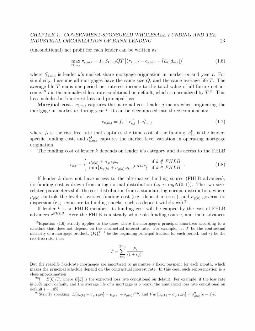
CHAPTER 1. GOVERNMENT-SPONSORED WHOLESALE FUNDING AND THEINDUSTRIAL ORGANIZATION OF BANK LENDING 23
(unconditional) net profit for each lender can be written as:
maxrk,m,t
πk,m,t = ImSk,m,tQT[(rk,m,t − ck,m,t − lEk[dm,t])
](1.6)
where Sk,m,t is lender k’s market share mortgage origination in market m and year t. Forsimplicity, I assume all mortgages have the same size Q, and the same average life T . Theaverage life T maps one-period net interest income to the total value of all future net in-come.19 l is the annualized loss rate conditional on default, which is normalized by T .20 Thisloss includes both interest loss and principal loss.
Marginal cost. ck,m,t captures the marginal cost lender j incurs when originating themortgage in market m during year t. It can be decomposed into three components:
ck,m,t = ft + cFk,t + cOk,m,t. (1.7)
where ft is the risk free rate that captures the time cost of the funding, cFk,t is the lender-specific funding cost, and cOk,m,t captures the market level variation in operating mortgageorigination.
The funding cost of lender k depends on lender k’s category and its access to the FHLB
ck,t =
{µg(k) + σg(k)ωt if k /∈ FHLBmin{µg(k) + σg(k)ωt, c
FHLB} if k ∈ FHLB . (1.8)
If lender k does not have access to the alternative funding source (FHLB advances),its funding cost is drawn from a log-normal distribution (ωt ∼ logN(0, 1)). The two size-related parameters shift the cost distribution from a standard log normal distribution, whereµg(k) controls the level of average funding cost (e.g. deposit interest), and σg(k) governs itsdispersion (e.g. exposure to funding shocks, such as deposit withdraws).21
If lender k is an FHLB member, its funding cost will be capped by the cost of FHLBadvances cFHLB. Here the FHLB is a steady wholesale funding source, and their advances
19Equation (1.6) strictly applies to the cases where the mortgage’s principal amortizes according to aschedule that does not depend on the contractual interest rate. For example, let T be the contractualmaturity of a mortgage product, {Pt}T−1
0 be the beginning principal fraction for each period, and rf be therisk-free rate, then
T =
T−1∑t=0
Pt
(1 + rf )t.
But the real-life fixed-rate mortgages are amortized to guarantee a fixed payment for each month, whichmakes the principal schedule depend on the contractual interest rate. In this case, such representation is aclose approximation.
20 l = E[L]/T , where E[L] is the expected loss rate conditional on default. For example, if the loss rateis 50% upon default, and the average life of a mortgage is 5 years, the annualized loss rate conditional ondefault l = 10%.
21Strictly speaking, E[µg(k) + σg(k)ωt] = µg(k) + σg(k)e0.5, and V ar[µg(k) + σg(k)ωt] = σ2
g(k)(e− 1)e.

CHAPTER 1. GOVERNMENT-SPONSORED WHOLESALE FUNDING AND THEINDUSTRIAL ORGANIZATION OF BANK LENDING 24
are a substitute for lenders’ deposit funding when they suffer bad deposit shocks. cFHLB
is the spread that the FHLB charges over the risk free rate that includes term premium,operational expenses, and the cost of posting collateral. In this sense, it is the effective costof FHLB funding. For FHLB member lenders, FHLB advances cap their funding cost atthe level of ft + cFHLB. They will fund their mortgages with FHLB advances when theirinstantaneous deposit cost is higher than the cost of FHLB advances.
Default rate. dm,t is the default rate of borrowers in market m, which depends on localeconomic conditions. Here, we are not considering borrowers’ idiosyncratic risk (e.g. FICOand LTV) in pricing market specific baseline interest rates.
Motivated by the fact that different lenders respond to local economic shocks differently,as shown in Figure 1.11, this model assumes in a very parsimonious way that a lender’sperception of local economic conditions is a function of the lender’s size.
Ek[dm,t] = φg(k)ρ(dm,t−1 − δ) + δ, (1.9)
where ρ measures the persistence of the local default rate. δ is the national average levelof default rate. φ(·) is a monotonically decreasing function bounded by [0, 1]. It governsa lender’s perception of the local economic conditions, thus its responsiveness in pricingmortgages. We can see that if φ(·) = 0 (e.g., the big four national banks), the lender justprices their mortgage at the national default rate. On the other extreme where φg(k) = 1,the lender fully adjust its interest rate to account for local economic conditions.
This is a very parsimonious way to model lenders’ heterogeneous reaction to local shocks,but this representation can be well micro-founded. In appendix section A.3, I provide a microfoundation, which builds on the agency frictions between the lender management and localbranch managers, a la Stein (2002), and attributes national banks’ low responsiveness tolocal shocks to their great cost in verifying local branch managers’ report on local defaultprediction.
Equilibrium
In equilibrium, mortgage demand is characterized by borrowers’ choice of mortgage lenders,given the mortgage rates and lender service quality. Supply is characterized by the lenders’optimal decision on their offered interest rates. FHLB funding would affect the equilibriuminterest rates by capping the funding cost of the member banks. The lenders are hetero-geneous in two key dimensions: the cost structure (average cost and volatility), and theperception of the local default rate.
Mortgage Demand. Household i in marketmmaximizes its utility by choosing betweenall lenders available in the market. It also has the option not to borrow if its reservation valueis higher than that offered by any lender. The distributional assumption of the idiosyncraticpreference εi,k,m,t implies that the (conditional) probability that borrower i in market m atyear t chooses lender k follows the standard logit form, as the integrand in Equation (1.10).

CHAPTER 1. GOVERNMENT-SPONSORED WHOLESALE FUNDING AND THEINDUSTRIAL ORGANIZATION OF BANK LENDING 25
Integrating out the unobserved heterogeneity ζi gives us the market share of each lender:
Sk,m,t =
∫ζi
exp(−αirk,m,t + qk,m + ξk,m,t)
1 +∑Km
ι=1 exp(−αirι,m,t + qι,m + ξι,m,t)dF (ζi). (1.10)
Mortgage Supply. The lender would set the optimal interest rate to maximize itsexpected profit in Equation (1.6). Solving the first order condition, we get the optimalinterest rate
r∗k,m,t = ck,m,t︸ ︷︷ ︸Marginal cost
+ lEk[dm,t]︸ ︷︷ ︸Risk premium
+Sk,m,t∫
ζi
αi exp(−αirk,m,t+qk,m+ξk,m,t)(1+∑ι 6=k exp(−αirι,m,t+qι,m+ξι,m,t))
(1+∑Kmι=1 exp(−αirι,m,t+qι,m+ξι,m,t))2
dF (ζi)︸ ︷︷ ︸Markup
. (1.11)
The optimal interest rate has three components: lenders’ marginal cost, risk premium andmarkup. The marginal cost varies within year t due to deposit fluctuations. The markupdepends on the lenders’ market power.
1.8 Estimation and Results
The model is summarized by Equation (1.8), (1.11) and (1.10), and characterized by aset of demand parameters (α, γ, σα, qk,m), parameters in default prediction (ρ, φg(k)), lenders’funding cost structures (µg(k), σg(k)), and the cost of FHLB advances (cFHLB). In this section,I discuss the estimation procedures and identification strategies.
Estimation and Identification
Estimation proceeds in two steps. In the first step, I estimate demand parameters usingdata on mortgages originated across the US. In the second step, I estimate the supplyparameters by targeting the FHLB effect in the reduced-form exercise, as well as othernecessary moments.
Demand Estimation
I use mortgages originated between 2000 and 2015 from my HMDA-Attom-McDash mergedsample to estimate the demand parameters. Since I only have the baseline interest ratesfor each lender in my structural model, I first residualize the mortgage rates using Equation(1.3), where I factor out borrower and product characteristics, including credit scores, LTV,lien status and interest type. I then aggregate the mortgage level data to lender-market ob-servations. A market is defined at the level of CBSA-loan purpose, e.g., mortgage refinances

CHAPTER 1. GOVERNMENT-SPONSORED WHOLESALE FUNDING AND THEINDUSTRIAL ORGANIZATION OF BANK LENDING 26
in the city of San Francisco. Following Buchak et al. (2018b), this paper also separates mar-kets into mortgages originated for new purchases and mortgage refinances since a borrowerlooking for one type of mortgage financing is not looking for the other type. Borrowerscan choose between all lenders in the market. In each CBSA-year, I include two demo-graphic variables: log incomes and log house prices. Both variables are from the AmericanCommunity Survey (ACS).
To capture the extensive margin of mortgage lending, I define market size in the sameway as Buchak et al. (2018b). One tenth of the total number of households are looking forpurchase mortgages, and all mortgagors are in the market of mortgage refinance.
I estimate the demand parameters in two steps. In the first step, I rewrite the Equation(1.10) as
Sk,m,t =
∫ζi
exp(−γ(Di − D)rk,m,t − σαζirk,m,t + λk,m,t)
1 +∑Km
ι=1 exp(−γ(Di − D)rι,m,t − σαζirι,m,t + λι,m,t)dF (ζi). (1.12)
With a generalized method of moments (GMM), I search over the (γ, σα) parameter space tominimize the predicted and the observed market shares of lenders. Here λk,m,t is the market-year-lender fixed effects. In each GMM iteration, they are recovered by the contractionmapping method following Berry et al. (1995) and Nevo (2001). In the second step, we canrecover α and qk,m by running the regression:
λk,m,t = −αrk,m,t + qk,m + ξk,m,t. (1.13)
Identification strategy. The interest rates offered by lenders might be reacting tosome unobserved factors, which might bias the estimation in both steps of the estimation. Toresolve this endogeneity problem, I construct a list of instrumental variables to instrument forthe interest rates in both steps. First, I use the big four national banks’ national interest rateto instrument for their mortgage rates in the local markets, by noting the fact that nationalbanks apply the uniform pricing strategy across the nation. For example, JP Morgan’s localinterest rates in San Francisco are not reacting to the local demand factors, but are dictatedby JP Morgan’s national pricing strategy. I also use other lenders’ mortgage characteristicsto instrument for the lender’s own interest rates following Berry et al. (1995). Specifically, Iuse other lenders’ average proportion of fixed rate mortgages, and average LTV.
Supply Estimation
The estimation of supply side parameters is based on the optimal pricing equation. I as-sume lenders in the same category share the same cost and default perception parameters(µg(k), σg(k), φg(k)). This largely reduces the dimension of the parameter space, and increasesthe power of estimation. The tradeoff is that I ignore the heterogeneity of lenders within thesame category, which is a second order issue in this paper.
The estimation uses the simulated method of moments (SMM). Specifically, the optimalpricing formula (1.11) allows me to simulate the interest rates charged by all categories oflenders, from which we can calculate the model implied moments. By minimizing the distance

CHAPTER 1. GOVERNMENT-SPONSORED WHOLESALE FUNDING AND THEINDUSTRIAL ORGANIZATION OF BANK LENDING 27
between the model implied and empirical moments, I am able to estimate the supply sideparameters.
Identification strategy. The key parameter on the supply side is cFHLB, which deter-mines the effect of the FHLB on banks of different categories. My estimation procedure addsthe FHLB effect on member banks’ interest rates (for regional banks and community banks)in my reduced form into the targeting moments. The parameter cFHLB will be mostly iden-tified by these two moments (interest rate drops after joining the FHLB for regional banks,and community banks). I also add other moments from the data to discipline my structuralmodel, including the mean and variance of the interest rates offered from lenders in eachcategory and mortgage rate sensitivity to lagged local default rates. The former is mainlyused to identify the distribution parameters of lenders’ funding cost (µg(k), σg(k)), and thelatter is mainly used to discipline the default perception parameters (ρ, φg(k)).
Estimation Results
Figure 1.15 plots the estimated distribution of the funding cost for banks of different sizes,and the funding cost of FHLB advances. The black line represents the funding cost for thenational banks, the blue line is for regional banks, and the red line is for community banks.We can see the national banks’ funding cost is on average lower than the other two groupsof banks. This is due to multiple reasons. First, the national banks have a large networkof branches, which facilitates their deposit raising. Second, national banks are perceived tobe “too big to fail”, so the depositors are more willing to put deposits into them if they areconcerned with the downside risk. This is especially important for their uninsured deposits(Jacewitz and Pogach, 2018; Egan et al., 2017). Other than the lower average funding cost,the national banks’ cost distribution is also tight due to their well diversified deposit base,so they are less exposed to funding shocks. So the idiosyncratic deposit withdraws would netout in their branch network. This can also be due to their many private wholesale fundingsources, including their many secondary market funding facilities (e.g. repo funding, assetbacked commercial papers). The regional banks’ cost distribution shifts towards the right,representing their higher funding costs, and the community banks’ cost distribution shiftsright even further.
Given this funding cost heterogeneity, the FHLB will have different effects on banks ofdifferent sizes, with a larger impact on community banks and less on national banks. Thenumerical simulation implies that the FHLB would effectively reduce the funding cost by 1basis point for national banks, by 15 basis points for regional banks, and by 28 basis pointsfor community banks. The effect looks smaller than what appears in the figure due to thecompetition in the market. In the market, lenders with higher funding costs would havesmaller marker share, thus its effective weight in calculating the FHLB effect is smaller.
Here I want to point out that the cost of FHLB advances is mainly identified using thereduced form effect on regional banks and community banks. We actually cannot observenational banks in the reduced form sample. The structural model enables me to recover the

CHAPTER 1. GOVERNMENT-SPONSORED WHOLESALE FUNDING AND THEINDUSTRIAL ORGANIZATION OF BANK LENDING 28
funding cost for the banks of all sizes, with which we can extrapolate the FHLB effect onnational banks.
Model Fit
Figure 1.16 compares the empirical and the simulated interest rate distribution for banks ofdifferent sizes. Overall the model fits the data well along the three dimensions: the mean,dispersion, and responsiveness to local defaults of the interest rates. The main limitationis that the model is not able to capture the non-linearity of interest rates in markets withvery low default rates. This is due to the linear assumption of banks’ perception of the localeconomic conditions.
1.9 Counterfactual Analysis
In this section, I use the estimated model to study two counterfactual policy changes re-garding the FHLB. The baseline is the current equilibrium, where more than 90% of banksare FHLB members, and the FHLB offers the same funding rate for all members. In thesecounterfactual policy environments, I evaluate the effect on aggregate mortgage originations,interest rates, as well as the market structure. With the structural model, we can also drawconclusions on the empirically unobserved outcomes, including borrowers’ welfare and thepass-through of the cost reduction due to government intervention.
Counterfactual 1: An Economy without the FHLB
To fully capture the impact of the FHLB in the economy, I first study the case where theFHLB does not exist. In the reduced form exercise, we are only able to observe a partialequilibrium exercise that one local bank joins the FHLB. Such a change would have a smallereffect on the aggregate outcomes, including mortgage originations and interest rate, since theaffected bank is only a small part of the market. As for the effect on the market structure, thecomparison can go in either direction. On the one hand, only one bank’s funding structureis changed, so the effect on the market structure is smaller. On the other hand, the affectedbank tends to be small, and it pushes the market to be more competitive without anyoffsetting forces. If we change the funding structure for both small and big lenders, theremight be an offsetting force to push the market to become more concentrated since the biglender also benefits from the FHLB. In this section, I am going to employ my structuralmodel to quantify the effect of the FHLB in a general equilibrium setting.
The simulation implies that if the FHLB is removed from the economy, the averagemarket interest rate would increase by 11 basis points, and aggregate mortgage originationswill fall by 7.05%. A simple back-of-the-envelope calculation suggests that national mortgage

CHAPTER 1. GOVERNMENT-SPONSORED WHOLESALE FUNDING AND THEINDUSTRIAL ORGANIZATION OF BANK LENDING 29
originations will decrease by $129.28 billion, and borrowers will have to pay $13.55 billionmore in interest payments.22
The impact of removing the FHLB is different for banks of different sizes, as shown inFigure 1.17. Community banks will be hurt the most, their interest rates will increase by 29basis points, and they will therefore lose market share of 4%. The regional banks’ mortgagerates will increase by 16 basis points, which would lead to a market share loss of 2%. Thenational banks, on the other hand, will benefit from the removal of the FHLB. Their interestrates will rise by 1 basis point, and they will have a market share increase of 2%. Thelack of the low-cost wholesale funding gives the national banks’ an advantageous position inthe market since there is less competition. The measure of market concentration, HHI, willincrease by 2.38 percentage points.
Figure 1.18 plots average market-level interest rates across markets with different localeconomic conditions. The x-axis is the local default rate in the past two years, and they-axis is the average baseline mortgage rates for all lenders.23 The solid line plots the pricingschedule for the current equilibrium with the FHLB, which is upward sloping, indicating thelenders are actively responding to the local economic conditions. The dashed line representsthe same relation in the counterfactual without the FHLB. In this case, the responsivelenders (community and regional banks) lose some market share, and the uniform pricers(national banks) are more dominating. As a result, the market responsiveness to localeconomic conditions falls, so we see a flatter slope. This would have negative consequences. Adecreased price responsiveness raises the degree of cross-subsidization from the safer marketsto the riskier markets. This would increase the high-default markets’ representation in thelending landscape, and raise the default rate at the aggregate level. Such a price distortionwould suppress the aggregate credit supply.
My structural model also allows me to directly calculate borrowers’ welfare, and it showsthe borrower will lose 10.28% of welfare. The is due to a higher level of interest rates, anda constrained credit supply.
Counterfactual 2: The FHLB Offers Member Banks DifferentPrices
The large effect of the FHLB suggested by the first counterfactual exercise is due to the tworoles that the FHLB plays in addressing market imperfections: shielding banks from liquidityshocks (the direct effect) and providing equal external funding access (the competition effect).Since the direct effect could also be achieved by the private market (e.g., warehouse lending),the competition effect is more informative for the value of public provision of wholesalefunding.
22The back-of-the-envelope takes the aggregate statistics in 2018 as the baseline. In 2018, the aggregateresidential mortgage origination is $1833.79 billion, and the total outstanding balance of the residentialmortgage is $12.32 trillion.
23The interest rate does not include borrower- and product-characteristic rate premiums.

CHAPTER 1. GOVERNMENT-SPONSORED WHOLESALE FUNDING AND THEINDUSTRIAL ORGANIZATION OF BANK LENDING 30
To isolate the competition effect of the FHLB, I consider a second counterfactual wherethe FHLB still exists, but chooses to offer different prices to different banks. The prices fordifferent banks are made so that the average funding cost of FHLB member banks is thesame as in the current equilibrium, but the market structure is the same as if there was noFHLB in the first counterfactual (orange bars in Figure 1.17). Therefore, this counterfactualhas the same cost reduction as in the current equilibrium. The only difference is the marketstructure in the mortgage lending, so this exercise would capture the effect of government-sponsored wholesale funding due to the shift of the industrial organization of the lendingmarket. Figure 1.19 plots the offered price of FHLB advances for the three groups of banks:CFHLBN is for national banks, CFHLB
R is for regional banks, and CFHLBC is for community
banks.The results show that if the FHLB were to apply this price schedule, aggregate mortgage
origination would drop by 2.46%, banks’ markup would rise by 3 basis points, and borrowers’welfare would drop by 3.76%. A simple back-of-the-envelope calculation implies that theFHLB’s impact on the industrial organization of the mortgage market increases mortgagelending by $50 billion and saves borrowers $4.7 billion in interest payments every year.
1.10 Conclusion
In testimony before Congress, Mike Menzies, the vice chairman of the Independent Com-munity Bankers of America (ICBA), said “the FHLBanks provide members advances forliquidity and asset/liability management... This access allows our members to offer the samehome mortgage products to our customers that the largest firms offer to theirs.” This papertakes an empirical approach, and illustrates that Federal Home Loan Banks are indeed play-ing a crucial role in supporting banks’ mortgage lending. Specifically, the FHLB providesbanks with low-cost wholesale funding, which eases their financial constraints, thus enablingthem to lower interest rates and issue more mortgages. What is more, the flexible structureof wholesale funding improves their ability to manage interest rate risk, and enables themto offer more fixed-rate products.
More interestingly, FHLB-funded small banks have substantial spillover effects on creditmarkets. First, the FHLB funding shifts the market structure and makes it more competitive.As a result, the market level interest rates fall, and the aggregate mortgage lending increasessignificantly. The second spillover effect is on pricing efficiency. Since the small banks arebetter at processing local information, they are very responsive to local economic shocks.After the FHLB increases the representation of small banks, more regional risk factors areincorporated into mortgage pricing, which makes credit more efficiently allocated.
I use a structural model to quantify the macro effect of the FHLB, and find that the FHLBincreases mortgage originations by $130 billion and saves the borrower $13 billion in interestpayments every year. The FHLB plays two roles in the economy. First, as an alternativefunding source, the FHLB protects the individual banks from idiosyncratic funding shocks,and thus reduces their funding cost (the direct effect). Second, the FHLB levels the playing

CHAPTER 1. GOVERNMENT-SPONSORED WHOLESALE FUNDING AND THEINDUSTRIAL ORGANIZATION OF BANK LENDING 31
field for small banks, which improves market competition and facilitates the pass-through ofcost reduction (the competition effect). My model enables me to quantify both effects, andshow that the competition effect alone accounts for a substantial part of the overall effect.The shift of the competitive landscape of the mortgage market alone leads to an annualincrease of mortgage originations of $50 billion, and an annual decrease of $4.7 billion ininterest payments.

CHAPTER 1. GOVERNMENT-SPONSORED WHOLESALE FUNDING AND THEINDUSTRIAL ORGANIZATION OF BANK LENDING 32
Figures
Figure 1.1 Illustration of Treated and Control Banks in an Example Merger
#
D
!
! !
!
! Illinois National Bank (Aquirer)D Palmer Bank (non FHLB)# Pleasant Plains State Bank (FHLB)
Census Tract 2000
0 8 164 Miles
1
Note: This is a multiple-target merger from my sample, that serves as an example to illustrate theintuition of the identification strategy. This merger happened in 2003. The acquirer (blue dots) IllinoisNational Bank simultaneously merged two target banks: Palmer Bank and Pleasant Plains State Bankin the suburban area of Springfield, Illinois. The treated bank branch (cross) was not able to tap intoFHLB advances before the merger, but could do so thereafter, while the control bank branch (triangle)already had FHLB access. Aside from this, both target branches experience similar organizationalchange due to the merger. Therefore, the within-merge difference-in-differences strategy could identifythe effect of getting access to wholesale funding provided by FHLB.Source: FDIC, FHFA, GIS.

CHAPTER 1. GOVERNMENT-SPONSORED WHOLESALE FUNDING AND THEINDUSTRIAL ORGANIZATION OF BANK LENDING 33
Figure 1.2 The Time Distribution of the Sample Multiple-Target Mergers
1998 2000 2002 2004 2006 2008 2010 2012 20140
5
10
15
20
25
30
Num
ber o
f Mul
tiple
Tar
get M
erge
rs
Note: This figure plots the number of sample multiple-target mergers over different years. All samplemergers satisfy the following conditions: (1) the acquirer merges at least two effective targets in thesame year; (2) the target is effective, if it does not belong to the same bank holding company withacquirer, and it has at least one branch that exists at least 4 years around the merger; (3) the acquirer isan FHLB member before mergers, and there is at least one FHLB member and at least one non-FHLBmember in its effective target banks.Source: FDIC, FHFA.

CHAPTER 1. GOVERNMENT-SPONSORED WHOLESALE FUNDING AND THEINDUSTRIAL ORGANIZATION OF BANK LENDING 34
Figure 1.3 The Geographical Distribution of Target Branches
Non FHLB Target Branches (Treated) FHLB Target Branches (Control)
Note: This figure plots the branch locations of the target banks in the treated (cross) and control(triangle) groups.Source: FDIC, FHFA, GIS.

CHAPTER 1. GOVERNMENT-SPONSORED WHOLESALE FUNDING AND THEINDUSTRIAL ORGANIZATION OF BANK LENDING 35
Figure 1.4 Effect of FHLB Funding on Mortgage Originations
<=-6 -4 0 4 >=810
5
0
5
10
15
20
25
Num
ber o
f Mor
tgag
e Or
igin
atio
ns
FHLB Effect CI--90% Balanced Panel
10
0
10
20
30
40
Scal
ed b
y Av
erag
e Le
vel a
t Per
iod
-1 (%
)
Note: This figure plots the effect of FHLB funding access to lenders’ mortgage originations, obtainedfrom estimating Equation (1.1). The left y-axis measures the effect in absolute mortgage originations,and the right y-axis rescales the effect by the baseline mortgage originations at event year -1. Theregression controls event-year fixed effect, event-branch fixed effect, county-year fixed effect, as wellas a battery of variables, including tract median income, home ownership, minority fraction, educatedfraction and mortgagor fraction. The bars plot 90% confidence intervals for each point estimate. Robuststandard errors are clustered at the event level.Source: FDIC, FHFA, HMDA, author’s own calculations.

CHAPTER 1. GOVERNMENT-SPONSORED WHOLESALE FUNDING AND THEINDUSTRIAL ORGANIZATION OF BANK LENDING 36
Figure 1.5 Effect of FHLB Funding on Mortgage Originations of Different Business Models
(a) Securitized Mortgages
<=-6 -4 0 4 >=87.5
5.0
2.5
0.0
2.5
5.0
7.5
10.0
Num
ber o
f Sec
uriti
zed
Mor
tgag
e Or
igin
atio
ns
FHLB Effect CI--90% Balanced Panel
20
10
0
10
20
30
40
Scal
ed b
y Av
erag
e Le
vel a
t Per
iod
-1 (%
)
(b) Mortgages Held on Balance Sheet
<=-6 -4 0 4 >=87.5
5.0
2.5
0.0
2.5
5.0
7.5
10.0
12.5
Num
ber o
f Bal
ance
She
et M
ortg
age
Orig
inat
ions
FHLB Effect CI--90% Balanced Panel
20
10
0
10
20
30
Scal
ed b
y Av
erag
e Le
vel a
t Per
iod
-1 (%
)
Note: This figure plots the effect of FHLB funding access to lenders’ mortgage originations, obtainedfrom estimating Equation (1.1). Panel (a) depicts securitized mortgages, and panel (b) illustratesthe mortgages that are held on banks’ balance sheet. The left y-axis measures the effect in absolutemortgage originations, and the right y-axis rescales the effect by the baseline mortgage originationsat event year -1. The regression controls event-year fixed effect, event-branch fixed effect, county-yearfixed effect, as well as a battery of variables, including tract median income, home ownership, minorityfraction, educated fraction and mortgagor fraction. The bars plot 90% confidence intervals for eachpoint estimate. Robust standard errors are clustered at the event level.Source: FDIC, FHFA, HMDA, author’s own calculations.

CHAPTER 1. GOVERNMENT-SPONSORED WHOLESALE FUNDING AND THEINDUSTRIAL ORGANIZATION OF BANK LENDING 37
Figure 1.6 Effect of FHLB Funding on Mortgage Interest Rate
<=-6 -4 0 4 >=8
0.6
0.4
0.2
0.0
0.2
0.4
0.6
Mor
tgag
e In
tere
st R
ate
(%)
FHLB Effect CI--90% Balanced Panel
10
5
0
5
10
Scal
ed b
y Av
erag
e Le
vel a
t Per
iod
-1 (%
)
Note: This figure plots the effect of FHLB funding access to lenders’ mortgage interest rates (%),obtained from estimating Equation (1.1). The left y-axis measures the effect in absolute mortgage rate,and the right y-axis rescales the effect by the baseline mortgage rate at event year -1. The regressioncontrols event-year fixed effect, event-branch fixed effect, county-year fixed effect, as well as a batteryof variables, including tract median income, home ownership, minority fraction, educated fraction andmortgagor fraction. The bars plot 90% confidence intervals for each point estimate. Robust standarderrors are clustered at the event level.Source: FDIC, FHFA, HMDA, Attom, McDash, author’s own calculations.

CHAPTER 1. GOVERNMENT-SPONSORED WHOLESALE FUNDING AND THEINDUSTRIAL ORGANIZATION OF BANK LENDING 38
Figure 1.7 Effect of FHLB Funding on Mortgage Profile
10 5 0 5 10Composition Change (%)
FRM
ARM
Other
>550
550~600
600~650
650~700
700~750
750~800
>800
<60%
60%~80%
80%~100%
>100%
InterestType
FICO
LTV
Note: This figure plots the effect of FHLB funding access to the composition change of mortgageprofiles along interest type, FICO and LTV, obtained from estimating Equation (1.2). The dependentvariable is the proportion of the originating mortgages in each category. The regression controls event-year fixed effect, event-branch fixed effect, county-year fixed effect, as well as a battery of variables,including tract median income, home ownership, minority fraction, educated fraction and mortgagorfraction. The bars plot 90% confidence intervals for each point estimate. Robust standard errors areclustered at the event level.Source: FDIC, FHFA, HMDA, Attom, McDash, author’s own calculations.

CHAPTER 1. GOVERNMENT-SPONSORED WHOLESALE FUNDING AND THEINDUSTRIAL ORGANIZATION OF BANK LENDING 39
Figure 1.8 Effect on Market Concentration in the Local Census Tract
<=-6 -4 0 4 >=84
3
2
1
0
1
2
HHI o
f the
Loc
al M
ortg
age
Mar
ket (
%)
FHLB Effect CI--90% Balanced Panel
Note: This figure plots the effect to HHI of the local mortgage market after a local small bank joinsFHLB, obtained from estimating Equation (1.1). The market is defined as the 2000 census tractwhere the bank branch is located. The regression controls event-year fixed effect, event-branch fixedeffect, county-year fixed effect, as well as a battery of variables, including tract median income, homeownership, minority fraction, educated fraction and mortgagor fraction. The bars plot 90% confidenceintervals for each point estimate. Robust standard errors are clustered at the event level.Source: FDIC, FHFA, HMDA, author’s own calculations.

CHAPTER 1. GOVERNMENT-SPONSORED WHOLESALE FUNDING AND THEINDUSTRIAL ORGANIZATION OF BANK LENDING 40
Figure 1.9 Effect on Aggregate Mortgage Originations in the Local Census Tract
<=-6 -4 0 4 >=820
10
0
10
20
Mor
tgag
e Or
igin
atio
ns o
f the
Cen
sus T
ract
FHLB Effect CI--90% Balanced Panel
10
5
0
5
10
15
Scal
ed b
y Av
erag
e Le
vel a
t Per
iod
-1 (%
)
Note: This figure plots the effect to market mortgage originations after a local small bank joins FHLB,obtained from estimating Equation (1.1). The market is defined as the 2000 census tract where the bankbranch is located. The regression controls event-year fixed effect, event-branch fixed effect, county-yearfixed effect, as well as a battery of variables, including tract median income, home ownership, minorityfraction, educated fraction and mortgagor fraction. The bars plot 90% confidence intervals for eachpoint estimate. Robust standard errors are clustered at the event level.Source: FDIC, FHFA, HMDA, author’s own calculations.
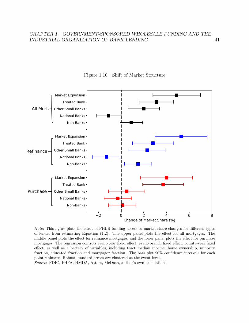
CHAPTER 1. GOVERNMENT-SPONSORED WHOLESALE FUNDING AND THEINDUSTRIAL ORGANIZATION OF BANK LENDING 41
Figure 1.10 Shift of Market Structure
2 0 2 4 6 8Change of Market Share (%)
Market ExpansionTreated Bank
Other Small BanksNational Banks
Non-Banks
Market ExpansionTreated Bank
Other Small BanksNational Banks
Non-Banks
Market ExpansionTreated Bank
Other Small BanksNational Banks
Non-Banks
All Mort.
Refinance
Purchase
Note: This figure plots the effect of FHLB funding access to market share changes for different typesof lender from estimating Equation (1.2). The upper panel plots the effect for all mortgages. Themiddle panel plots the effect for refinance mortgages, and the lower panel plots the effect for purchasemortgages. The regression controls event-year fixed effect, event-branch fixed effect, county-year fixedeffect, as well as a battery of variables, including tract median income, home ownership, minorityfraction, educated fraction and mortgagor fraction. The bars plot 90% confidence intervals for eachpoint estimate. Robust standard errors are clustered at the event level.Source: FDIC, FHFA, HMDA, Attom, McDash, author’s own calculations.

CHAPTER 1. GOVERNMENT-SPONSORED WHOLESALE FUNDING AND THEINDUSTRIAL ORGANIZATION OF BANK LENDING 42
Figure 1.11 Regional Pricing Schedule for Banks of Different Sizes
(a) Non-GSE Mortgage Sample
0 1 2 3 4 5Local Default Rate in the Past 2 Years (%)
4.50
4.75
5.00
5.25
5.50
5.75
6.00
6.25
6.50
Risk
Adj
uste
d In
tere
st R
ate
(%)
National BanksRegional Banks
Community Banks(b) GSE Mortgage Sample
0 1 2 3 4 5Local Default Rate in the Past 2 Years (%)
4.50
4.75
5.00
5.25
5.50
5.75
6.00
6.25
6.50
Risk
Adj
uste
d In
tere
st R
ate
(%)
National BanksRegional Banks
Community Banks
Note: This figure plots the relationship between the residualized interest rate rit (y-axis) and the locallagged default rates dc(i),t (x-axis) for both non-GSE mortgages (panel a) and GSE mortgages (panelb). The national banks are the top 4 bank holding companies by their combined total assets. Theregional banks are all banks with total assets above $1 billion, except for the national banks. And thecommunity banks are all banks with total assets below $1 billion. The scatters represent the averagevalue for 50 percentiles for each group of banks.Source: FDIC, FHFA, Attom, McDash, author’s own calculations.

CHAPTER 1. GOVERNMENT-SPONSORED WHOLESALE FUNDING AND THEINDUSTRIAL ORGANIZATION OF BANK LENDING 43
Figure 1.12 Concentric Rings from the Target Branch
#*
D
LegendD Palmer Bank (non FHLB)
Illinois National Bank#* Pleasant Plains State Bank (FHLB)
Census Tract 2000
Note: This sample merger happened in 2003. The acquirer Illinois National Bank simultaneouslymerged two target banks: Palmer Bank and Pleasant Plains State Bank in the suburban area ofSpringfield, Illinois. The width of each ring belt is 2 miles.Source: FDIC, FHFA, GIS.

CHAPTER 1. GOVERNMENT-SPONSORED WHOLESALE FUNDING AND THEINDUSTRIAL ORGANIZATION OF BANK LENDING 44
Figure 1.13 FHLB Effect on Mortgage Lending Over Space
5 0 5 1020
10
0
10
20
30
40
Mort
gage C
ount
per
square
mile
Geographic Distribution of Treatment Effect
Effect on Mortgage Count within 2mi
CI--95%
5 0 5 1020
10
0
10
20
30
40
Mort
gage C
ount
per
square
mile
Geographic Distribution of Treatment Effect
Effect on Mortgage Count from 2mi to 4mi
CI--95%
5 0 5 1020
10
0
10
20
30
40
Mort
gage C
ount
per
square
mile
Geographic Distribution of Treatment Effect
Effect on Mortgage Count from 4mi to 6mi
CI--95%
5 0 5 1020
10
0
10
20
30
40
Mort
gage C
ount
per
square
mile
Geographic Distribution of Treatment Effect
Effect on Mortgage Count from 6mi to 8mi
CI--95%
5 0 5 1020
10
0
10
20
30
40
Mort
gage C
ount
per
square
mile
Geographic Distribution of Treatment Effect
Effect on Mortgage Count from 8mi to 10mi
CI--95%
Note: This figure plots the effect on mortgage lending across different concentric rings. The resultsare obtained from estimating Equation (1.1). The bars plot 95% confidence intervals for each pointestimate. Robust standard errors are clustered at the event level.Source: FDIC, FHFA, HMDA, McDash, author’s own calculations.

CHAPTER 1. GOVERNMENT-SPONSORED WHOLESALE FUNDING AND THEINDUSTRIAL ORGANIZATION OF BANK LENDING 45
Figure 1.14 Effect of FHLB Funding on Small Business Loan Originations
<=-6 -4 0 4 >=820
10
0
10
20
Num
ber o
f Sm
all B
usin
ess L
oans
FHLB Effect CI--90% Balanced Panel
60
40
20
0
20
40
60
Scal
ed b
y Av
erag
e Le
vel a
t Per
iod
-1 (%
)
Note: This figure plots the effect of FHLB funding access to lenders’ small business loan originations,obtained from estimating Equation (1.1). The left y-axis measures the effect in absolute mortgageoriginations, and the right y-axis rescales the effect by the baseline mortgage originations at event year-1. The regression controls event-year fixed effect, event-branch fixed effect and county-year fixed effect.The bars plot 90% confidence intervals for each point estimate. Robust standard errors are clusteredat the event level.Source: FDIC, FHFA, CRA, author’s own calculations.

CHAPTER 1. GOVERNMENT-SPONSORED WHOLESALE FUNDING AND THEINDUSTRIAL ORGANIZATION OF BANK LENDING 46
Figure 1.15 Estimates of Funding Cost
-1 -0.5 0 0.5 1 1.5 2Marginal Funding Cost (%)
0
0.1
0.2
0.3
0.4
0.5
Note: This figure plots the offered price of FHLB advances for the three groups of banks: CFHLBN is
for national banks, CFHLBR is for regional banks, and CFHLB
C is for community banks.

CHAPTER 1. GOVERNMENT-SPONSORED WHOLESALE FUNDING AND THEINDUSTRIAL ORGANIZATION OF BANK LENDING 47
Figure 1.16 Model Fit of Mortgage Interest Rates
(a) Empirical Interest Rates
0 1 2 3 4 5Local Default Rate in the Past 2 Years (%)
4.50
4.75
5.00
5.25
5.50
5.75
6.00
6.25
6.50
Risk
Adj
uste
d In
tere
st R
ate
(%)
National BanksRegional Banks
Community Banks
(b) Simulated Interest Rates
0 1 2 3 4 5Local Default Rate in the Past 2 Years (%)
4.50
4.75
5.00
5.25
5.50
5.75
6.00
6.25
6.50
Risk
Adj
uste
d In
tere
st R
ate
(%)
Big Four BanksRegional Banks
Community BanksLinear Fit

CHAPTER 1. GOVERNMENT-SPONSORED WHOLESALE FUNDING AND THEINDUSTRIAL ORGANIZATION OF BANK LENDING 48
Figure 1.17 Counterfactual 1: Shift of Market Structure after Removing FHLB
National Regional Community0
5
10
15
20
25M
arke
t Sha
re (
%)
CurrentNo FHLB
Note: This figure plots the market share of banks of different sizes for the simulated equilibrium withFHLB (blue) and the counterfactual without FHLB (orange).

CHAPTER 1. GOVERNMENT-SPONSORED WHOLESALE FUNDING AND THEINDUSTRIAL ORGANIZATION OF BANK LENDING 49
Figure 1.18 Counterfactual 1: Average Mortgage Rates across Different Areas
0 1 2 3 4 5
Local Default Rate in the Past 2 Years (%)
1.9
2
2.1
2.2
2.3
2.4
2.5
2.6
Ave
rage
Inte
rest
Rat
e (%
)
CurrentNo FHLB
Note: This figure plots market mortgage rates across markets with different local economic conditionsfor the simulated equilibrium with FHLB (solid line) and the counterfactual without FHLB (dash line).

CHAPTER 1. GOVERNMENT-SPONSORED WHOLESALE FUNDING AND THEINDUSTRIAL ORGANIZATION OF BANK LENDING 50
Figure 1.19 Counterfactual 2: FHLB Advance Price Schedule
-1 -0.5 0 0.5 1 1.5 2Marginal Funding Cost (%)
0
0.1
0.2
0.3
0.4
0.5
Note: This figure plots the cost of FHLB advances relative to the estimated funding cost for the threegroups of banks. The black line and FHLB advance rate CFHLB
N are for national banks, the blue lineand CFHLB
R are for regional banks, and the red line and CFHLBC are for community banks. The price
schedule is made so that the average funding cost is the same as in the current equilibrium, but themarket structure is the same as if there were no FHLB in the first counterfactual (orange bars in Figure1.17).

CHAPTER 1. GOVERNMENT-SPONSORED WHOLESALE FUNDING AND THEINDUSTRIAL ORGANIZATION OF BANK LENDING 51
Tables
Table 1.1 Sample Descriptive Statistics
Non FHLBTarget
FHLB TargetDifference
within Mergerp-value
(1) (2) (3) (4)
Panel A: Sample Size
Multi-Target Mergers 174
Target Banks 250 254
Target Branches 2051 1170
Panel B: Target Bank Characteristics Before Mergers (Unit: $Million)
Total Asset 13,735 13,969 11,587 [0.19](86,543) (104,154) (8,749)
Total Deposit 9,068 9,452 5,662 [0.26](58,849) (69,608) (5,009)
Total Lending 7,890 8,468 5,959 [0.21](47,297) (57,534) (4,743)
Non-Performing Loan Ratio 0.01 0.02 -0.00 [0.86](0.02) (0.02) (0.00)
Loan Loss Ratio 0.02 0.02 0.00 [0.42](0.01) (0.01) (0.00)
Real Estate Ratio 0.60 0.65 -0.02 [0.15](0.25) (0.26) (0.02)
C&I Ratio 0.16 0.14 -0.00 [0.90](0.11) (0.10) (0.01)
Branch Count 112 114 39 [0.42](589) (602) (49)
Panel C: Census Tract Characteristics in 2000 Census
Median Income 45,101 46,842 -731 [0.70](20,327) (21,454) (1,864)
House Unit 2,231 2,380 39 [0.64](1,131) (1,494) (82)
Home Ownership 0.62 0.64 -0.01 [0.36](0.22) (0.22) (0.01)
Minority Fraction 0.20 0.18 0.02 [0.11](0.20) (0.18) (0.01)
Educated Fraction 0.65 0.64 0.01 [0.58](0.18) (0.18) (0.02)
Mortgagor Fraction 0.69 0.69 -0.00 [0.99](0.15) (0.16) (0.01)
# of Bank Branches 4.32 5.02 -0.48 [0.14](3.88) (4.73) (0.33)
Note: This table summarizes the characteristics of the sample banks and their locating census tracts.Column (3) displays the difference within each merger event. Column (4) reports the p-value of thetest that the corresponding difference is 0. Standard deviations/errors are in parentheses. ∗ p < 0.10,∗∗ p < 0.05, ∗∗∗ p < 0.01.Source: FDIC, FHFA, GIS, FFIEC.

CHAPTER 1. GOVERNMENT-SPONSORED WHOLESALE FUNDING AND THEINDUSTRIAL ORGANIZATION OF BANK LENDING 52
Table 1.2 FHLB Effect on Banks of Different Sizes
Mortgage Originations Mortgage Interest Rate (%)
(1) (2) (3) (4)
FHLB9.76∗∗∗ -0.181∗∗
(2.84) (0.076)
relative to baseline 16.3% -3.2%
FHLB×Regional9.20∗∗ -0.164∗∗
(3.72) (0.079)
relative to baseline 15.2% -2.7%
FHLB×Community11.78∗∗∗ -0.292∗∗∗
(4.23) (0.095)
relative to baseline 20.7% -4.3%
Event-Year FE X X X XEvent-Branch FE X X X XCounty-Year FE X X X X
Obs. 62,260 62,260 56,099 56,099
Note: This table reports the effect of FHLB funding access to mortgage originations and rates, obtainedfrom estimating Equation (1.2). Column (1) and (3) report the average effect for the full sample, whilecolumn (2) and (4) report effect for regional banks (total assets above $1 billion) and community banks(total assets below $1 billion), respectively. Below the point estimate, the row “relative to baseline”includes the size of the effect relative to the baseline of each outcome variable at event year -1. Theregression controls event-year fixed effect, event-branch fixed effect, county-year fixed effect, as wellas a battery of variables, including tract median income, home ownership, minority fraction, educatedfraction and mortgagor fraction. Standard errors in parentheses are clustered at the event level. ∗
p < 0.10, ∗∗ p < 0.05, ∗∗∗ p < 0.01.Source: FDIC, FHFA, HMDA, Attom, McDash, author’s own calculations.

CHAPTER 1. GOVERNMENT-SPONSORED WHOLESALE FUNDING AND THEINDUSTRIAL ORGANIZATION OF BANK LENDING 53
Table 1.3 Effect of FHLB Funding on Market Interest Rates
DependentVariable
Local Market Treated BankOther
Lenders
OtherLenders
(NationalBanks)
OtherLenders
(Small andNon-
Banks)
(1) (2) (3) (4) (5)
FHLB -0.083∗∗ -0.181∗∗ -0.074∗ -0.031 -0.093∗
(0.037) (0.076) (0.042) (0.052) (0.049)
Event-Year FE X X X X X
Event-BranchFE
X X X X X
County-Year FE X X X X X
Cluster Event Event Event Event Event
Obs. 152,658 56,099 96,329 29,830 66,499
Note: This table reports the effect to the market interest rates of the mortgages after a local bank joinsFHLB, obtained from estimating Equation (1.2). Column (1) reports the effect for all lenders in thelocal market. Column (2) reports the effect for the treated banks, while column (3) reports the effectfor lenders except for the treated banks. Column (4) illustrates the effect for national banks that are inthe same market with the treated banks, column (5) focused on small banks (regional and communitybanks) and non-banks in the same market with the treated banks. The regression controls event-yearfixed effect, event-branch fixed effect, county-year fixed effect, as well as a battery of variables, includingtract median income, home ownership, minority fraction, educated fraction and mortgagor fraction.Standard errors in parentheses are clustered at the event level. ∗ p < 0.10, ∗∗ p < 0.05, ∗∗∗ p < 0.01.Source: FDIC, FHFA, HMDA, Attom, McDash, author’s own calculations.

CHAPTER 1. GOVERNMENT-SPONSORED WHOLESALE FUNDING AND THEINDUSTRIAL ORGANIZATION OF BANK LENDING 54
Table 1.4 Effect of FHLB Funding on Market Mortgage Rates (Triple Diff)
DependentVariable
Market Mortgage Rates (%)
Safe Market Risky Market Full Sample Non-GSE GSE Loans
(1) (2) (3) (4) (5)
Post×FHLB×Good
Market
-0.037∗ -0.048∗∗ -0.021
(0.019) (0.024) (0.016)
Post×FHLB -0.096∗∗ -0.065∗ -0.061∗∗ -0.097∗∗ -0.028
(0.045) (0.038) (0.030) (0.041) (0.023)
Event-Year FE X X X X X
Event-BranchFE
X X X X X
County-YearFE
X X X X X
Cluster Event Event Event Event Event
Obs. 2,303,434 2,405,784 4,709,218 2,820,510 1,888,688
Note: This table reports the effect to the market interest rates of in both good and bad marketsafter a local bank joins FHLB, obtained from estimating Equation (1.2). Column (1) and (2) still usethe difference-in-differences specification, and report the effect for safe and risky markets, receptively.Markets are defined as safe if it is located in a county where the mortgage default rates in the pasttwo years are below the national median. Column (3) further interact Post×FHLB with the indicatorof safe markets (triple diff). Column (4) and (5) apply the triple diff regression to GSE securitizedmortgages, and non-GSE securitized mortgages receptively. The regression controls event-year fixedeffect, event-branch fixed effect, county-year fixed effect, as well as a battery of variables, includingtract median income, home ownership, minority fraction, educated fraction and mortgagor fraction.Standard errors in parentheses are clustered at the event level. ∗ p < 0.10, ∗∗ p < 0.05, ∗∗∗ p < 0.01.Source: FDIC, FHFA, HMDA, Attom, McDash, author’s own calculations.
55
Chapter 2
Match-Fixing in the MortgageFinance Field: Credit Default Swapsand Moral Hazard
2.1 Introduction
The past few decades have witnessed a spectacular rise of the market for credit derivatives,such as credit default swaps (CDS). As the name suggests, these credit derivatives are largelyviewed as redundant securities or side bets, that do not have any influence on the underlyingassets. But in the public debates, it is not rare to hear that credit derivatives are blamedto cause trouble on the fundamental market. For example, mortgage CDS is still publiclyreferred to as one of the key drivers of the housing bubble in the early 2000.
In theory, the trading of credit derivatives would alter the incentives of market par-ticipants, and distort the fundamental outcomes (Bolton and Oehmke, 2011a; Parlour andWinton, 2013). Ex ante, the creditors might issue too much credit if they are able to insureagainst defaults through CDS trading. Mortgage CDS, in our example, swap out the defaultrisk from the mortgage backed security (MBS) investors, thus drive up their demand, loosentheir origination standards (Arentsen, Mauer, Rosenlund, Zhang, and Zhao, 2015), and ex-acerbate credit expansion to subprime borrowers. Ex post, given CDS participants’ profitis a function of the underlying assets’ performance, they would take actions to influence thefundamental outcomes. Similar moral hazard problems arise in the sports’ games, and wecould often see scandals where the gamblers bribe the referees or players to fix the matches.But whether this ex post distortion behavior is a significance phenomenon in the financialmarket remains unknown, to which an answer could contribute to the policy making pro-cess in the CDS market where different distortion behaviors have evoked close attention andpreventative actions from the regulators.1
1Concurrently, the debate gets quite contentious whether “naked” credit derivatives are allowed to betraded between those who do not have any interest on the underlying assets. The concern that the speculative

CHAPTER 2. MATCH-FIXING IN THE MORTGAGE FINANCE FIELD: CREDITDEFAULT SWAPS AND MORAL HAZARD 56
To fill in this knowledge gap, this paper explores the ex post moral hazard problems inthe subprime mortgage backed security (MBS) market, and empirically demonstrates theexistence the CDS protection alters the incentives of market participants, which affects theperformance of the underlying mortgages. Specifically, I find if there are CDS coveringa mortgage pool, the CDS sellers would help the mortgage borrowers to refinance, whichimmediately unloads the CDS sellers’ obligation to cover the loss of the underlying mortgages.Consequently, the mortgages in CDS referencing pools are more likely to be refinanced andless likely to default.
Using Moody’s Lewtan ABSNet database, I collect a sample of subprime residentialmortgages that were originated during 2003–2007, and securitized in the private label market.A mortgage is defined to be covered by CDS if it is securitized into a mortgage pool whichis backing at least one bond (tranche) that are referenced by at least one CDS contract.In the final sample, roughly 1/3 of the 8,559,650 subprime mortgages are covered by CDS.An regression analysis with an exhaustive list of control characteristics demonstrates thatCDC-covered mortgages are 3.6% more likely to refinanced, and 2.1% less likely to default.The differences sustain after controlling origination-year-by-CBSA fixed effect and mortgageservicer fixed effect.
An empirical challenge to the controlled regression analysis is that CDS sellers mightendogenously write CDS on mortgages that have greater potential to refinance. This couldbe the case if CDS sellers are better informed about the unobserved mortgage characteristics,which are correlated with the mortgage borrowers’ refinance behaviors. Then the observeddifferences between CDS-covered and non-CDS-covered mortgages are just driven by theCDS sellers’ superior information instead of ex post actions. To mitigate this concern, thispaper further explores the local randomization due to the discontinuous sale of mortgagesby their originators. At the start of the mortgage securitizaion process, the originatorsissue mortgage loans for their daily business. They then stack many mortgages issued overa period and sell a whole chunk at a lower frequency (e.g. every one or two months).I assume the characteristics (both observed and unobserved) of the mortgages are slowlymoving with time, and compare the mortgages originated just before and after the sale ofa mortgage chunk. Mechanically, the mortgages that are originated before the sale will fallinto a different mortgage pool from the ones originated right after. I then pick up the caseswhere the two mortgage pools have sharply different CDS coverage statuses and constructtwo balanced mortgage groups a la regression discontinuity design. Empirically, the treatedand control groups are balanced across all different mortgage and borrower characteristics,but the CDS covered mortgages have significantly higher rate of refinance, and lower rate ofdefault.
To better understand the mechanism of CDS seller’s ex post distortion, I further lookinto the financial networks between CDS sellers and mortgage servicers. I hypothesize ifthe CDS seller and the mortgage servicer are in the same financial holding company, the
use of credit derivatives might destabilize the market for the underlying asset motived EU to permanentlyban “naked” CDS trading for European sovereign debt in 2011.

CHAPTER 2. MATCH-FIXING IN THE MORTGAGE FINANCE FIELD: CREDITDEFAULT SWAPS AND MORAL HAZARD 57
refinancing behavior of the mortgage borrowers can be more easily influenced through theservicer channel. Indeed, the affiliation of the CDS seller and mortgage servicer has a sig-nificantly positive interactive effect on mortgage refinance and negative interactive effect onthe probability for loan default.
This paper provides the firsthand evidence to trace the outcome manipulation actions inthe mortgage finance market. This evidence illustrates that credit derivative trading mightgive rise to crucial moral hazard problems, that motivate the derivative traders to influencethe fundamental assets through ex post actions. For example, the change of the refinanceand default rate for the underlying mortgages has huge price impact on the related securities.All the mortgage related securities are highly structured, thus any small change of the deepparameters will be largely amplified, and compromise the benefits of related market investors.Beyond the mortgage market, such outcome manipulation threatens market fairness, anddistorts the hedging activities for other market participants. For example, if a pension fundwants to buy some mortgage CDS to hedge its overall exposure to housing market, it cannotachieve its goal. In particular, what it wants to hedge plummets, but what it uses as a hedgeoutperforms its hedged target because CDS seller has manipulated the performance of theunderlying pools.
Literature review. This paper mainly relates to two lines of research. First, it con-tributes to the literature on CDS and their effect on underlying asset performance. Servedas “side bets”, credit derivatives including CDS should not affect the underlying assets ina frictionless world. However, many theoretical works have shown these credit derivativescould potentially play a role given the existence of various frictions. Duffee and Zhou (2001)and Arping (2014) show that they increase the credit supply from creditors given asymmetricinformation between creditors and debtors. Parlour and Winton (2013) incorporates contractincompleteness, and finds that CDS lead to inefficient monitors from the creditors. Boltonand Oehmke (2011b) considers renegotiation friction and shows that CDS can help to reducethe incidence of strategic default. However, lenders will “overinsure” in equilibrium, givingrise to an inefficiently high incidence of bankruptcy. In the empirical literature, Sarettoand Tookes (2013) documents that firms with traded CDS can sustain higher leverage andborrow at longer debt maturities. Subrahmanyam, Tang, and Wang (2014) shows that theinception of CDS trading leads to higher credit risk of the referencing firm due to highercost of creditor coordination. This paper complements this line of literature by focusing onthe moral hazard friction ex post, and provides robust empirical evidence.
Second, this papers adds to the literature on the linkage between structured financeproducts and the housing market. Stulz (2010) provides a comprehensive discussion of therole of CDS in the recent financial crisis, and points out while many financial institutionsincur huge losses in CDS trading, the primary drivers of the crisis are the financial institu-tions’ misjudgment and misconduct. However, the prevalent securitization practice in themortgage market has been shown to reduce the mortgage lenders’ incentive to screen theirborrowers (Keys, Mukherjee, Seru, and Vig, 2010; Purnanandam, 2011). Arentsen et al.(2015) directly investigates the CDS market, and argues that CDS coverage leads to higher

CHAPTER 2. MATCH-FIXING IN THE MORTGAGE FINANCE FIELD: CREDITDEFAULT SWAPS AND MORAL HAZARD 58
default of subprime mortgages. This paper is the first in the literature to identify the out-come manipulation actions in the mortgage finance market, and shows that the CDS marketparticipants directly influence the mortgage borrower behaviors after origination.
Overview. The paper proceeds as follows. Section 2.2 discusses the data and theinstitutional setting for the US mortgage market. Section 2.3 outlines the empirical strategyand documents the main results with a regression framework. Section 2.4 leverages a localrandomization strategy to rule out the ex ante selection by the CDS sellers. In section 2.5,I employ interactive regressions to explore the mechanism of the CDS sellers’ manipulationof mortgage performance. Section 2.6 concludes.
2.2 Institutional Background and Data Description
Institutional Background
The US mortgage market is characterized by the prevalence of securitization, which is seen asthe most important financial innovation in the past few decades. After origination, mortgageloans are not usually held to maturity by the originators, which are usually banks, creditunions, or mortgage companies. Instead, a fast-growing share of mortgages are pooled andsold to financial intermediaries for securitization. During the securitization process, the cashflows from the mortgage pools will be structured into different bonds, or mortgage backedsecurities (MBS), and sold to final investors. Usually, different bonds have different senioritiesand different degrees of risk according to their priority to receive cash flows. Typical finalinvestors include pension funds, hedge funds, banks, and foreign financial institutions.
Before the financial crisis, there were two major mortgage securitization markets accord-ing to the types of financial intermediaries: agency MBS and private-label MBS. AgencyMBS are securitized by three government or quasi-government agencies: Ginnie Mae, FannieMae, and Freddie Mac. These entities are either explicitly or implicitly backed by the fullfaith and credit of the US government,2 and they provide guarantees to MBSs that theyissue. Thus, agency MBSs are de facto free from credit risk. Private-label MBS are, instead,securitized by private financial institutions. Before the housing bust, large investment bankswere very active in securitizing “subprime” mortgages, whose lenders either have very lowcredit scores or lack income documentation.3
As opposed to agency MBS investors, private-label MBS buyers must assume the creditrisk of the underlying mortgages. However, they can choose to enter into a credit default
2Ginnie Mae bonds are backed by the full faith and credit of the US government. While Fannie Mae andFreddie Mac securities lack this same backing, a majority of the investors believe that these two agencies arebacked by implied federal guarantee. This belief was realized when the government bailed them out in themid of the financial crisis.
3These mortgages do not conform to government agency guidelines, thus cannot be securitized by thegovernment agencies. Before the crisis, many scholars (Mian and Sufi, 2009) believe the growing demand forMBSs drive the expansion of credit to subprime borrowers and a boom of private-label MBS market.

CHAPTER 2. MATCH-FIXING IN THE MORTGAGE FINANCE FIELD: CREDITDEFAULT SWAPS AND MORAL HAZARD 59
swap (CDS) contract, which has been widely used in the corporate bond and sovereign bondmarket, to swap out the credit risk. A CDS contract works as an insurance on the underlyingsecurities. In the case of underlying mortgage defaults, which lead to cash flow shortfall intheir backed securities, the CDS seller, or the de facto insurer, will compensate the CDSbuyer any cash flow shortfall, in exchange for a flow of fixed insurance premiums paid bythe CDS buyer. Contrary to an ordinary insurance contract, the buyers do not have to holdinsurable interests to enter into a CDS contract. CDS buyers can be the investors of theunderlying MBS or some other investors that are betting on bad performance of the housingmarket. In some cases, the notional value of the CDS contracts can be multiple times aslarge as the underlying MBS because many CDS buyers do not hold any insurable interests.This actually increases CDS sellers’ exposure to the default risks and elevates their incentiveto improve the performance of the underlying mortgages, which exacerbates the match fixingphenomenon in the mortgage market.
An Anecdotal Match-Fixing Example
There is an anecdotal story in which a Texan brokerage firm, Amherst Holdings, managedto manipulate the mortgage payment to avoid default payments on CDS contracts it hadsold to the investment banks (Zuckerman, Ng, and Rappaport, 2009). In 2009, AmherstHoldings sold CDS to the investors to guarantee the payment of a mortgage pool with atotal balance of $27 million. The CDS contacts were sold to many investors, who did nothave insurable interest, but wanted to short the housing market. The CDS buyers includeJPMorgan Chase, Royal Bank of Scotland, and Bank of America. And the total bet (notionalamount) reached $130 million, which was almost 5 times as high as the total balance of theunderlying mortgage pool. Since it was deep in the financial crisis, the market was expectingthat more than 90% of the underlying mortgage would default. Thus Amherst Holdings wasable to collect premium payment worth more than $100 million, which was much more thanthe total balance of the mortgages it guaranteed.
In the end, Amherst Holdings took $27 million and paid back the principals for all theunderlying borrowers, in which way all its insured obligation was immediately cleaned up.4
And it still kept tens of millions dollars as its profit. While this case is quite extreme, itdoes exemplify that the CDS position might incentivize the CDS sellers to fix the mortgageperformance ex post, given it directly affects their profit. And the goal of this paper is totest whether similar match-fixing behaviors are a significant phenomenon in the subprimemortgage market.
4Normally a third party cannot pay off loans directly for the mortgage borrowers. But if the amountof outstanding loans falls to less than 10% of the original pool, which was the case in this example, themortgage servicer—or company that collects mortgage payments from homeowners and forwards them toinvestors who own the securities—can buy them and make bondholders whole.

CHAPTER 2. MATCH-FIXING IN THE MORTGAGE FINANCE FIELD: CREDITDEFAULT SWAPS AND MORAL HAZARD 60
Data
I use Moody’s Lewtan ABSNet database to construct a sample of subprime5 residential mort-gages originated from 2003 to 2007.6 Lewtan ABSnet is an industry leading data source thatprovides extensive performance metrics and origination information on almost all privatelysecuritized mortgages. For each loan, we can observe the loan amount, securitization amount,combined loan-to-value (CLTV) ratio, credit score, prepayment penalty status, loan type,lien status, purchase purpose and documentation status, at the point of origination. Also,we can track each loan’s payment history, and tell whether a loan is current, prepaid ordefaulted at any month after origination.
To identify the reasons for prepayment, I supplement the Lewtan ABSnet data withATTOM, which contains detailed property ownership and associated home loan informationfrom the public records. At the property level, ATTOM records all ownership transfers anddetailed information on the associated mortgages, including loan amount, interest rate type,and distress indicator.
Following Griffin and Maturana (2016) and Bartlett et al. (2018), I merge ABSnet withATTOM through a matching algorithm.7 Subprime mortgages from Lewtan ABSnet arematched with loan records in ATTOM if they agree with loan amount, origination date,termination date, default status and interest rate type. The algorithm successfully matchesmore than 63% of the prepaid mortgages, among which 60% are considered high qualitymatches.
For the purpose of this paper, I categorize the merged prepaid subprime mortgages (2.66million) in Lewtan ABSnet into three groups according to their prepayment motivation. Aprepaid mortgage is classified as moving (0.33 million) if there is at one real sale happeningwithin 2 months around the prepayment date for the linked property in ATTOM. If theborrower is not moving and he or she takes out at least one new loan collateralized bythe same property within 2 months around the prepayment date, the prepaid mortgage isclassified as refinance (1.91 million). The rest of the prepaid mortgages are classified asnormal pre-payoff (0.42 million).
Summary Statistics
Our final data sample contains 8,559,650 subprime mortgages in 4,756 mortgage pools thatare originated during the 2003–2007 period. The number of the mortgage pools in this pa-per is very close to that in Arentsen et al. (2015), where they explore the LoanPerformancedatabase from CoreLogic. Roughly 1/3 of the mortgage pools are covered by CDS protec-tions, as can be seen from panel A of Table 2.1. The proportion of mortgage pools with
5Subprime mortgages are defined as those that back private-label mortgage-backed securities marketedas subprime, as in Mayer and Pence (2008) and Palmer (2015).
6This paper focuses on 2003 to 2007 period as in Arentsen et al. (2015), for it includes more than 90%(need to be verified) of the subprime mortgages that are ever issued
7I thank Justin Chiang and Paulo Issler for their tremendous help with the matching process.

CHAPTER 2. MATCH-FIXING IN THE MORTGAGE FINANCE FIELD: CREDITDEFAULT SWAPS AND MORAL HAZARD 61
CDS coverage is smaller than the level of 54.5% in Arentsen et al. (2015) since I do notobserve the CDS contracts expiring or terminated before 2012. So I might misclassify someCDS-covered mortgage pools as non-CDS-covered in the case that the mortgage pools werecovered by CDS, but the protection ended before 2012. This will mitigate the difference ofthe treated and control groups, and bias the observed effect of CDS coverage towards 0. Onthe other hand, the CDS-covered mortgage pools that I pick up tend to be longer positions,in which case the transaction participants have stronger incentives to influence the mortgageborrowers behaviors.
Panel B of Table 2.1 provides summary statistics for the borrowers and loans in oursample. Column (1) and (2) report the characteristics for non-CDS-covered and CDS-coveredsubsamples respectively. The CDS-covered mortgages are of similar size with those withoutCDS coverage. And the majority of the mortgage principal in the securitization pools aresecuritized for both subsamples. In the dimension of credit quality, the borrowers in theCDS-covered pools have slightly lower credit scores, since the investors in these mortgagesare more concerned about credit risk, and are more likely to demand CDS protection ontheir MBS positions. On average, the mortgage borrowers in our sample have relatively lowcredit scores, with average FICO of 625. This is consistent with the common perceptionfor the subprime mortgage borrowers. The borrowers in both subsamples have similar levelof cumulative loan-to-value ratio, with 1.9 percentage points lower for the borrowers in theCDS-covered mortgage pools.
As to contract features, CDS sellers tend to pick mortgages with no prepayment penaltyto underwrite protections on. The average proportion of the mortgages that have prepaymentpenalty in the CDS covered pools are 40.44%, 4.6 percentage points lower than those withoutCDS coverage. This strategic choice would reduce their cost to refinance these mortgagesafter origination. CDS investors also prefer adjustable rate mortgages (usually with lowerteaser rate in the beginning few years), whose borrowers are more likely to refinance whenthe interest rate resets to its normal level. Noticeably, fewer of the CDS-covered mortgageshave balloon payment features. Other than that, both categories have comparable levels ofinterest-only feature, first-lien status, investment purpose and documentation completeness.As consistent with other studies, the subprime mortgages in this paper have very low level offull documentation (53.58%), and high level of adjustable interest rate (66.31%). Other thanthat, the majority of the subprime mortgages are fist-lien mortgages and not for investmentpurposes, similar as in the prime mortgage market.
2.3 Main Results
In this part, I test the hypothesis that CDS sellers are encouraging the borrowers to refinancetheir mortgages after origination to reduce the default risk. Specifically, I demonstrate thatmortgages with CDS coverage are more likely to be refinanced and less likely to default.This result survives a variety of different specifications.

CHAPTER 2. MATCH-FIXING IN THE MORTGAGE FINANCE FIELD: CREDITDEFAULT SWAPS AND MORAL HAZARD 62
Regression Specification
I test the treatment effect of CDS coverage with the following regression specification (2.1).Yi is the outcome of the mortgages, and it can be mortgage prepayment, refinance, default,etc. DCDS
i is a dummy variable, which equals 1 if a mortgage is in a pool that is backing atleast one bond that some outstanding CDS are referencing, and 0 otherwise. Its coefficientβ measures the effect of CDS coverage on the corresponding outcome Yi. Xi incorporatesan exhaustive list of control variables to make the mortgages comparable in the observabledimensions. They include CLTV, credit score, loan purpose, as well as indicators of pre-payment penalty, interest only, balloon payment, ARM, first lien, investment house and fulldocumentation.
Yi = α + βDCDSi + γXi + εi (2.1)
To make sure the difference is not coming from CDS sellers’ strategic choice over geogra-phies or market timing, I also include origination year by CBSA fixed effect in my mainspecification. I also include mortgage servicer fixed effect to make sure the difference perfor-mance of the two subsamples are not driven by the facts that they are serviced by differentservicers. This paper chooses to cluster the standard errors at the mortgage pool level, sincethis is where the true variations come from.
Regression specification (2.1) applies the linear probability model to estimate the CDScoverage effect. In the implementation, I also apply the logit model as a robustness test.The results are very similar with the linear probability model, which indicates that thenon-linearity at the tail distribution is not first order.
Mortgages with CDS Coverage Have Higher Prepayment Rate
Table 2.2 demonstrates the estimation of the CDS coverage effect on mortgage prepaymentwith different regression specifications. Column (1) controls observed borrower and loancharacteristics and origination year fixed effects. To match geographical distribution ofthe mortgages, column (2) further includes core-based statistical area (CBSA) fixed effects.Column (3), instead, includes Origination Year × CBSA fixed effects to compare mortgagesonly originated in the same year and located in the same CBSA. I control servicer fixedeffects in specification (4) and resort to a logit model in column (5).
Across all different specifications, CDS coverage has a significantly positive effect onmortgage prepayment. Specifically, if I control the observed borrower and mortgage char-acteristics, as well as the origination year fixed effects in column (1), the point estimate ofthe CDS coverage effect is 5.4%. Column (2) and (3) further control CBSA fixed effects intwo different ways. But they barely change the result, which indicates that the CDS coveredmortgages do not distribute very differently from those not covered by CDS geographically.But if I further add the servicer fixed effects into the regression, the CDS coverage effectshrinks a bit to 4.2%. This is my preferred specification, since it accounts for the fact thatthe servicers for the mortgage pools that are covered by CDS are different from those not

CHAPTER 2. MATCH-FIXING IN THE MORTGAGE FINANCE FIELD: CREDITDEFAULT SWAPS AND MORAL HAZARD 63
covered by CDS. Column (4) shows that for two mortgage with similar characteristics, orig-inated to similar borrowers in the same year and same CBSA, and that are served by thesame servicer, the one with CDS coverage is 4.2% more likely to be prepaid in its life thanthe other that is not covered by CDS. For robustness, I also apply a logit model with thesame set of control variables in column (5), the result is of the same magnitude with thatthe linear probability model suggests.
Here prepayment is a general form of mortgage termination if the balance of the mortgageis paid off ahead of the schedule in the mortgage contract. Due to the special arrangement ofpayment (equal installment, or with various types of small deviations) and long-term featurefor mortgage contracts, the majority of the mortgages end up being prepaid if not defaulted.8
Prepayment can be motivated by three reasons. First, the majority of the prepayment takesthe form of refinancing. Refinancing can be for the purpose of lowering interest rates orcashing out from home equity. For borrowers who have adjusted-rate mortgages that offerlow initial “teaser” rates, they might want to use a new loan to replace their outstandingmortgage if they can reduce their effective mortgage rate. As opposed to the general mortgagepools, the majority of the subprime mortgages are adjustable rate, of which most have lowinitial “teaser” rates. So refinancing is also important for the borrowers in the subprimesample. Another important reason for refinancing is to borrow more from the same collateral,which is often referred to as “cash-out refinance”. Both types of refinancing are driven bycost reduction incentives. Second, a mortgage has to be prepaid if the borrowers choose tomove out from the collateralized house. This type of prepayment is usually driven by non-economic incentives, including job changes or other exogenous life events. Finally, mortgageprepayment could take place if the borrowers choose to pay off the remaining balance withouttaking out a new loan or moving. In the next subsection, I will break down the mortgageprepayment according to different reasons to see which channel is driving the prepaymentresults.
Mortgages with CDS Protection Are More Likely to BeRefinanced
By merging the mortgages in Lewtan ABSnet into the property information in ATTOM, Iam able to identify the reasons for mortgage prepayment. Precisely, if there is a ownershipchange of the property within 2 months around the mortgage prepayment date, I identify themortgage prepayment to be driven by moving. If there is not an ownership change duringthis period, and there is at least one new loan originated during this period, we can inferthe previous mortgage is replaced by new loans, and mark the prepayment as refinance. Therest of the prepayment activities are just normal pre-payoff by the borrowers.
8In my sample, 53% of the subprime mortgages are prepaid over their life. For prime mortgages, accordingFederal Housing Finance Agency (2018), 10–20% of the 30-year fixed-rate agency mortgages are prepaid everyyear.

CHAPTER 2. MATCH-FIXING IN THE MORTGAGE FINANCE FIELD: CREDITDEFAULT SWAPS AND MORAL HAZARD 64
In Table 2.3, I report the CDS coverage effect for each category of the mortgage prepay-ment. For each prepayment category, I apply both the linear probability model and logitmodel to estimate the CDS coverage effect, controlling borrower and loan characteristics,origination year by CBSA fixed effects, and servicer fixed effects.
We can see that almost all of the CDS coverage effect on prepayment is driven by mortgagerefinance. Mortgage pools with CDS coverage have 3.6% more mortgage refinance rate thanthose without CDS coverage, given other characteristics are identical. This difference dwarfsother two types of prepayment, including moving and normal pre-payoff. As we notice, theeffect of CDS coverage on moving-driven prepayment is marginally significant. The effectis very small, both statistically and economically. This effect is mainly due to propertyshort-sale, which is a preferred process to liquidate the borrowers’ properties (Zhang, 2018).In the case of mortgage distress, CDS sellers would also have an incentive to encourage theborrowers to short-sale his or her property to recover the most of collateral value. Theseshort-sale transactions will show up in the moving prepayment if the sale of the property isenough to cover the mortgage remaining balance.
Normal pre-payoff, as a control group, is not affected by the CDS coverage. This issupportive to the ex post manipulation channel, as opposed to the selection channel. Ifthe CDS sellers just pick up mortgages with unobservably good characteristics, instead ofexerting ex post effort to refinance the borrowers, we would expect to see the same effect onnormal payoff, which is not the case in the data.
Table 2.4 reports the CDS coverage effect on mortgage refinance using different regressionspecifications. Similar with mortgage prepayment, CDS coverage consistently contributes tomortgage refinance by about 4 to 6 percentage points. This result is robust across originationyear, geographic area and servicer controls. With the preferred specification in column (4),a mortgage with CDS coverage is 3.6% more likely to be refinanced than those without CDScoverage.
Will the mortgage borrowers’ decision influenced by a third party? To answer this ques-tion, we need to understand a little background about how refinance works in practice. Asexplained in the last subsection, mortgage borrowers choose to refinance to lower their ef-fective interest rate, or to extract more debt from their home collateral. The literature haspointed out that the mortgage borrowers under-explore refinance opportunities to lower theireffective interest rate, especially for the poorer and less educated borrowers. There are manyreasons for the inertia for the borrowers to react to the rate-reducing incentives. An impor-tant one is that the decision to refinance a mortgage is challenging for many households, sothe borrowers need to be financially literate enough to make the right decision. And theborrowers need to pay certain fee for the refinancing processing, which might be difficultfor liquidity constrained borrowers. Campbell (2006) documents 12–14% of households werepaying more than 2 percentage points above the prevailing mortgage interest rate in the late1990s and early 2000s; this figure rose above 25% in 2003 after steep drops in interest ratesmade refinancing particularly advantageous. So in practice, many third parties, includingmortgage originators, servicers, or other lending competitors, would nudge the borrowers torefinance, by marketing calls/emails, or other advertisement campaigns. Although costly,

CHAPTER 2. MATCH-FIXING IN THE MORTGAGE FINANCE FIELD: CREDITDEFAULT SWAPS AND MORAL HAZARD 65
these refinance “reminders” are the mortgage originators’ or servicers’ fiduciary duty, as wellas a good investment since refinancing could generate origination profit for the originatorsof new loans.
The intensity of the refinance reminders would be mortgage-dependent, and it will affectthe likelihood of refinancing for the borrowers. The results in Table 2.4 show that if themortgage is securitized into a mortgage pool whose performance determines the payoutof some CDS contract, the CDS sellers will influence the refinance reminding intensity toincrease the refinance rate for the borrowers in their pools. In the later sections, I will exploremore on which parties would help them implement this strategy.
CDS-Covered Mortgages Default Less
Finally, let us look at how CDS coverage would affect mortgage default performance. Sincegreater proportion of mortgages are refinanced in the CDS covered pools, we can expect themortgage default would be less. Table 2.5 verifies this premise.
Table 2.5 shows the mortgages with CDS coverage tend to have about 2% lower defaultrate than those without CDS. This result is robust after controlling mortgage and borrowercharacteristics, origination year, CBSA and mortgage servicers. Both linear probability andlogit models suggest the same conclusion. The CDS sellers’ strategy of refinancing is effectiveso that it indeed moves some risky borrowers out of the mortgage pools that they cover,and lower the corresponding default rate. The reduction of the default rate is statisticallysignificant and economically meaningful.
Before I move to how the CDS sellers are able to implement this refinancing strategy, letme briefly discuss the efficiency of this refinance strategy. In a typical subprime mortgagepool from my data sample, 53% of the borrowers (prepayers) end up prepaying their mort-gages, 29% (defaulters) choose to default, and the rest 18% (normal borrowers) pay backtheir mortgage as scheduled. If the CDS sellers were able to perfectly distinguish the borrow-ers and pinpoint the ones they prefer for refinancing, the most efficient strategy for them isto target all defaulters. With this first-best strategy, all incremental refinanced borrowers aredefaulters, there should be a one-to-one relationship between refinance increase and defaultdecrease. So the first-best strategy would lead to a 3.6% decrease of the mortgage default.But our observed default decrease is 2.1% with the preferred specification in column (4) ofTable 2.5, which indicates the practical efficiency is lower than the first-best scenario. Ac-tually, the first-best strategy does demand some unrealistic requirement on the CDS sellers.To implement this strategy, they need to acquire enough information to perfectly predicteach borrower’s performance. So the efficiency of the first-best strategy should be thoughtof as a upper bound on any practical implementation of the refinancing strategy.
Now let us consider another random-refinance strategy, where the compliant refinancedborrowers are a random sample from the mortgage pool. With this strategy, the incremen-tal refinanced borrowers are a mix of defaulters and normal borrowers, and their relativedistribution is the same as the mortgage pool (29:18). In this case, the incremental 3.6%refinancers consist of 62% defaulters and 38% normal borrowers. And the realized default

CHAPTER 2. MATCH-FIXING IN THE MORTGAGE FINANCE FIELD: CREDITDEFAULT SWAPS AND MORAL HAZARD 66
decrease should be 2.2%, which is still larger than our observed level of default rate decrease.To interpret this result, let us think of under what circumstance the random-refinance strat-egy can be implemented. For example, if the CDS sellers do not have any information on themortgage borrowers, but randomly mail refinance pamphlets and coupons to the mortgageborrowers, and all the borrowers have the same probability of compliance to use the couponsto refinance their mortgages. This would lead to a 2.2% decrease of the mortgage rate.The CDS sellers could increase their efficiency from this benchmark by targeting more likelydefaulters based on their inside information. But there is the other force driving down theefficiency if the defaulters’ compliance probability is lower than the normal borrowers, whichis very likely since defaulters are more liquidity constrained and have more moral hazardproblems. In an extreme case that the defaulter never comply to CDS sellers’ refinancingpromotions, the default rate would not change. The observed lower efficiency level suggeststhat the second unequal-compliance force slightly dominates the first targeting force. But asignificant decrease of default rate tells us that some defaulters did comply to CDS sellers’actions.
2.4 Casual Analysis with Local Randomization
In section 2.3, I compare the mortgages with and without CDS coverage using a regres-sion framework and controlling an exhaustive list of observed variables. The results showcompelling patterns of strong CDS effects. Even if I have controlled many mortgage charac-teristics, as well as origination year, CBSA and servicers, there might be some unobservedcharacteristics that are observed and used by the CDS sellers. In that case, the observeddifference in refinance and default performance is due to ex ante selection, instead of ex postactions.
To rule out the selection story, this part further explores the local randomization due tothe discontinuous sale of mortgages by their originators to achieve more convincing identifica-tion. At the start of mortgage securitizaion process, the originators issue mortgage loans fortheir daily business. They then stack many mortgages issued over a period and sell a wholechunk at a lower frequency (e.g. every one or two months). I assume the characteristics(both observed and unobserved) of the mortgages are slowly moving with time, and comparethe mortgages originated just before and after the sale of a mortgage bulk. Mechanically, themortgages that are originated before the sale will fall into a different mortgage securitizationpool from the ones originated right after. I then pick up the cases where the two mortgagepools have sharply different CDS coverage statuses and construct two balanced mortgagegroups a la regression discontinuity design.
Local Randomization Around Mortgage Sales
Figure 2.1 depicts mortgage origination counts for a specific originator from the beginningof 2003 to the mid of 2004. It aims to serve as an example to illustrate how mortgage

CHAPTER 2. MATCH-FIXING IN THE MORTGAGE FINANCE FIELD: CREDITDEFAULT SWAPS AND MORAL HAZARD 67
origination and sale works. The length of the bars marks the volume of mortgage originationfor different dates. The bars with the same color represent the mortgages in the samesecuritization pool. And we can clearly see this originator focuses on one specific mortgagepool during one period. On average, this originator is issuing about 200 mortgages on adaily basis. But it does not sell the loans all the time. Instead, it stacks the originatedmortgages in its inventory, and sells a whole bulk very 2 months. The date of the mortgagesale is called “cutoff date” by the practitioners. For this specific originator, we can tell fromthis figure that its cutoff date is on the first date of very odd month. As a result, we canroughly see the color is changing every 2 months.
The potential local randomization comes from the cutoff date, around which the twogroups of mortgages are very much comparable, but fall into different mortgage pools, thusmight have different CDS coverage statuses.
The black dash line plots the realized proportion of CDS coverage for the mortgagesin each date. Here it is important to point out that the mortgages in the same pool havethe same CDS coverage status by definition. In the case of this mortgage originator, themortgages sold before October 31, 2003 were not covered by CDS, which the mortgage poolssold after that date happened to have CDS coverage.
We will compare the mortgages issued just before the cutoff date October 31, 2003 (con-trol group), and those issued right after (treated group). And the local randomization comesfrom the discontinuous change of the CDS coverage at this cutoff date. Our identificationassumption is that the characteristics of the issued mortgages are slowly moving with time.Under this assumption, the mortgages issued on October 30 or 31 do not significantly dif-ferent from those issued on November 1 or 2. But the realized CDS coverage statuses aresharply different for the control and treated groups. The CDS coverage status of the con-trol group is inherited from the whole black pool, and the treated group is inheriting CDScoverage from the teal pool. There might be many reasons that the black pool and the tealpool have different CDS coverage statuses. Maybe the investors of the teal pool were hit bysome exogenous shocks that encouraged them to buy CDS protection. Or maybe the marketknew the mortgages were getting worse with time due to the ever loosening origination stan-dard, thus the later mortgage pools were perceived to be riskier, and need CDS protection.However, this would not harm our identification, since the pool level decisions were madebased on the average mortgages in that pool, while I focus on a small window of originationdates overlapping the two mortgage pools. As long as the origination standard was slowlyrelaxed, the treated and control groups should be fairly comparable.
Detecting Cutoff Dates and Constructing the LocalRandomization Sample
Mortgage originators sell a bulk of mortgages at sparsely distributed cutoff dates, whichcreates an opportunity for identification. But the exact cutoff dates are not observed. Inpractice, there is no industry standard set of cutoff dates. Instead, the cutoff dates are chosen

CHAPTER 2. MATCH-FIXING IN THE MORTGAGE FINANCE FIELD: CREDITDEFAULT SWAPS AND MORAL HAZARD 68
by individual originators separately. Moreover, not every cutoff date is useful to identify theCDS coverage effect. If the mortgage pools on the two sides of the cutoff date are bothcovered by CDS, or either is covered, there would not be any variations that can be used toidentify the CDS effect.
To detect useful cutoff dates, I develop a algorithm that aims to address both of aboveproblems simultaneously. For each mortgage originator k at each day t, I compute the shareof mortgages that ex post have CDS coverage sCDSct . Then the useful cutoff dates will be theset of dates that have daily absolute changes of CDS coverage share above some threshold s.
Ek = {(k, t) : |sCDSkt − sCDSkt−1 | ≥ s} (2.2)
For a reasonably large s, the dates that fall in Ek are extremely likely to be cutoff dates,since we would except a close to zero change of the CDS coverage share unless the mortgagesoriginated on the two consecutive dates fall in different mortgage pools. For example, inFigure 2.1 I plot the sCDSct for this specific originator with the black dash line. For anydates inside a bulk of colored area, the dash line never jumps sharply. If an originator doesnot have this “originate daily and sell bulks at cutoff dates” model, there would not besharp pool switches, and the mortgage CDS coverage share should not jumps sharply either.This algorithm also rules out less useful cutoff dates by definition. Mechanically, the set ofidentified cutoff dates require the CDS coverage change larger than s. In the example ofFigure 2.1, only 2003-11-01 and 2004-05-01 will be included, while other clearly seen cutoffdates will not be included into Ek because of CDS coverage changes less than s.
The choice of s involves some discretion. A small s would mistakenly include someundesired and less powerful dates, while a large s would restrict the size of the data sample.In this paper, I set s = 0.5. With this choice, I am able to pick up 87 originator-cutoff-datepairs. I call each pair an event. So the event set is the union of identified cutoff dates fromall originators.
E(s) = ∪kEk(s) (2.3)
For each event (k, t), I collect all mortgages originated by k in the time window [t −5, . . . , t, . . . , t + 5]. To facilitate the regression exercises in the later part, I reorder thecalendar dates for a subset of the events. Actually, the identified events can be grouped intotwo categories according to the sign of the CDS coverage changes (sCDSkt − sCDSkt−1 ). A positiveshare difference means the mortgages after the cutoff dates have more CDS coverage ex post,while a negative share difference indicates the opposite. To make this more similar to a evenstudy framework, I reverse the date order for the cutoff dates with negative share difference,so the treated group always falls on the right side of the cutoff dates.
Table 2.6 reports summary statistics for the 26,372 mortgages in the identified localrandomization sample (the set of loans originated within 5 days of each of the detectedcutoff dates) used in estimation. Panel A reports loan and borrower characteristics, whichare very similar with those in the full sample as reported in Table 2.1. Panel B summarizesthe outcome variables, including prepayment (refinance, moving, normal pre-payoff) and

CHAPTER 2. MATCH-FIXING IN THE MORTGAGE FINANCE FIELD: CREDITDEFAULT SWAPS AND MORAL HAZARD 69
default. Different from the full sample, the overall prepayment rate in this sample is lower,and the default rate is slightly higher. Here we can see that the prepayment is brokendown into three categories according to the reasons. But the sum of their means (25%) arenot equal to the overall prepayment rate (36%). This is because the breakdown is doneby merging ABSnet with ATTOM, but not all mortgages can be successfully merged. Themissing 9% is due to the failed merges.
First-Stage Results
To validate my research design, I present a series of diagnostics designed to test whethermy local randomization sample meets the two main identifying assumptions required forvalid estimation. First, similar with the regression discontinuity design, the probability oftreatment (i.e., CDS coverage) is discontinuous at detected cutoff dates. Second,a validdesign requires that any borrower and loan characteristics (observed or unobserved) thatcould influence loan outcomes change only continuously at the cutoff dates. This smoothnesscondition requires that borrowers on either side of a cutoff date are otherwise similar, suchthat borrowing outcomes on either side of a cutoff date would be continuous absent thedifference in treatment induced by the sale of a bulk of mortgages at the cutoff date.
Figure 2.2 plots the average CDS coverage share for mortgages in the short window aroundthe identified cutoff dates, which demonstrates the time pattern of the CDS coverage. Itillustrates the smoothness in the conditional expectation function except for the cutoff date,at which we can clearly see a sudden jump of the CDS coverage status. This figure confirmsthe slow moving feature of CDS coverage, and the sudden switch due to the bulk sale ofmortgages at cutoff dates.
To formally estimate the average magnitude of the CDS coverage discontinuity acrossthe cutoff dates, I resort to a regression discontinuity regression.
DCDSikt∗+τ = β1τ + δ1(τ ≥ 0) + β2τ1(τ ≥ 0) + αkt∗ + γXik + εikt∗+τ (2.4)
for any originator-cutoff-date pair (k, t∗) in E(s). DCDSikt∗+τ is the dummy variable equal to
one if mortgage i originated by lender k at τ days after (or −τ days before) the cutoff datet∗ is covered by CDS ex post. It will be replaced by other outcome variables (e.g. othermortgage characteristics and performance) in the reduced form regressions. 1(τ ≥ 0) is anindicator variable equal one if the mortgage i is originated after the cutoff date (τ > 0,or treated). αkt∗ controls the event fixed effect, and Xik controls the loan and borrowercharacteristics, origination year by CBSA fixed effects and the servicer fixed effects, as inEquation (2.1). In this specification, δ is the key coefficient and quantifies the size of CDScoverage shock due to the fact that the mortgages on the two sides of the cutoff dates fallinto different mortgage pools that happen to have different CDS coverage statuses, althoughthey are otherwise similar mortgages.
Table 2.7 reports the results of this exercise. The mortgages that are originated rightafter the identified cutoff dates are 61.4% more likely to have CDS coverage than the mort-gages originated just before. This is a very strong first stage result, mainly due to the fact

CHAPTER 2. MATCH-FIXING IN THE MORTGAGE FINANCE FIELD: CREDITDEFAULT SWAPS AND MORAL HAZARD 70
that I restrict the cutoff dates to having CDS coverage differences above 50%. This wouldprovide quasi-exogenous variations with great power to identify the effect of CDS coverageon mortgage performance.
Quasi-Randomness Test
To verify our identification assumption that other loan characteristics beside CDS coveragedo not change discontinuously at the cutoff dates, Figure 2.3 plots the average value ofa few loan-level characteristics that might affect mortgage performance by the originationdates around the cutoffs. I plot the sample means and associated 95% confidence intervalsalong with fourth-order polynomial robust functions estimated following Calonico, Cattaneo,and Titiunik (2014). From panel A to F, I display borrower credit score, cumulative loan-to-value ratio, loan balance at origination, prepayment penalty indicator, interest only indicatorand full documentation indicator, respectively. These plots indicate smoothness in ex anteborrower and loan characteristics around the cutoff dates. Mortgages originated on bothsides of the cutoff dates do not appear statistically different in terms of their credit quality,debt capacity or other contract features.
Table 2.8 uses the specification in Equation 2.4 replacing the outcome variables with the 6loan characteristics in Figure 2.3 to report the magnitude and significance of the discontinuitycoefficients on these variables using the loan-level data. The estimates in column (1) indicateno statistical difference in credit scores for borrowers on either side of the threshold. Column(2) shows that cumulative loan-to-value ratios of borrowers on either side of the thresholdsare statistically indistinguishable. Column (3) looks at the loan amounts granted to theborrowers, and suggests that the sizes of the mortgages are not statistically different on eitherside of the cutoff dates. Column (4) suggests borrowers just before and after the cutoff dateshave similar proportion of investment purpose. Column (5) investigates a detailed contractfeature for the mortgages, and shows that mortgages originated across the cutoff dates havestatistically indistinguishable level of interest-only feature. Also, they have indistinguishableproportion of full documentation.
While the CDS coverage proportion is sharply different across the identified cutoff dates,borrowers on either side of these cutoff dates are demographically similar and apply forsimilarly sized loans with similar characteristics, supporting the validity of the identificationstrategy.
Causal Effect of CDS Coverage on Mortgage Refinancing
By quasi-randomly assigning mortgages into different mortgage pools, the cutoff disconti-nuities represent exogenous variations in their CDS coverage. Next I document empiricallythat borrowers on the side with more CDS coverage will be influenced to refinance morethan those on the other side.
Figure 2.4 provides visual evidence of the different prepayment performance for mort-gages originated across the cutoff dates by plotting proportion of different types of prepaid

CHAPTER 2. MATCH-FIXING IN THE MORTGAGE FINANCE FIELD: CREDITDEFAULT SWAPS AND MORAL HAZARD 71
mortgages for left- and right-of-threshold borrowers using the local randomization strategy.Panel A plots the proportion of the refinanced mortgages. As in the first-stage estimation,the gray dots represent the sample means for mortgages originated in each day around thecutoff dates, and the solid lines are the fitted forth-degree polynomial functions for eitherside. Refinance proportion is smooth leading up to the cutoff date, and then jumps up dis-continuously at the cutoff date, which demonstrates a strong causal effect of CDS coverageon mortgage refinancing performance. Panel B plots the proportion of prepaid mortgagesdue to moving incentives, and panel C plots that of normal prepayment. Consistent withthe results I have shown in section 2.3, the CDS coverage has at most weak influence onmortgages’ prepayment due to moving and normal prepayment.
As before, I estimate Equation (2.4) by controlling for mortgage characteristics, origina-tion year by CBSA fixed effects and servicer fixed effects using a bandwidth of 5 days aroundthe mortgage sale cutoff dates with a triangle kernel. Column (1) of Table 2.9 presents thereduced form results. Mortgages originated right after the mortgage sale cutoff are 4.9%more likely to be refinanced after origination. Since the mortgages are otherwise similaracross the cutoff dates, which has been shown extensively in the quasi-randomness test, thecause of the different refinancing performance can only be attributed to the fact that themortgages originated right after the cutoff dates happen to be sold to mortgage pools withhigher level of CDS coverage. To quantify the causal effect of the CDS coverage, I resortto two-stage least square estimation. Column (2) shows that CDS coverage will lead to anincrease of refinance rate by 8%. This is statistically significant, and is slightly larger thanthe controlled regression estimates in section 2.3 with the full sample.
Column (3) and (4) report the reduced form and two-stage least square estimates forprepayment due to moving. The difference around the cutoff dates is not significant. So wecan conclude that the CDS coverage has little effect on this type of prepayment. Intuitively,the CDS sellers’ advertisement campaigns are effective to remind the mortgage borrowers torefinance, but turn out not very effective to push them to move to other houses. Column (5)and (6) report the results for normal prepayment, and the difference is statistically significantfor the case with the bandwidth of 5 days. But this is not a robust result for different choicesof bandwidth. As can been seen in panel C of Figure 2.4, the average proportion of normalprepayment right before the mortgage sale cutoff dates appears to be abnormally lower thanthat after the cutoff dates, as well as that originated a few days before. It bends the trenddownward sharply, likely due to some idiosyncrasies in the data. If I se a larger bandwidth,the difference significance around the cutoff dates disappears.
Causal Effect of CDS Coverage on Mortgage Default
To further test my second hypothesis that CDS sellers are able to reduce the mortgage defaultrate by improving the refinance rate, Figure 2.5 displays the different default performancefor mortgages originated across the cutoff dates using the same strategy. Similar as in therefinance performance, the average default rate is smoothly moving for mortgages originatedon either side of the cutoff dates, but there is a striking jump at the mortgage sale cutoff
CHAPTER 2. MATCH-FIXING IN THE MORTGAGE FINANCE FIELD: CREDITDEFAULT SWAPS AND MORAL HAZARD 72
dates. The quasi-random setup allows us to conclude this default rate difference is due tothe different CDS coverage levels.
The precise estimates are presented in Table 2.10. The mortgages originated right afterthe cutoff dates have default rates 4.5 percentage points lower than the otherwise similarmortgages originated before the cutoff dates. As long as the exclusion condition satisfies, thisdefault performance difference can only be ascribed to the 61.4-percentage-point differencein their CDS coverage levels. Column (2) consolidates these two quantities, and illustratesthat a one-percentage-point increase of CDS coverage would lead to a 0.074-percentage-pointdecrease of the default rate. This is larger than the controlled regression estimates in section2.3 with the full sample.
2.5 Mechanism of Ex Post Distortion
The two sections above have illustrated clearly that the mortgages with CDS coverage havehigher probability to refinance, and lower probability to default. This is not due to exante selection but due to CDS sellers’ ex post manipulation. This section aims to betterunderstand the mechanics of the CDS sellers’ ex post influence.
CDS Sellers Fix Mortgage Performance Through MortgageServicers
In securitization, the mortgages are pooled together in common ownership held by a trust.The trust passively collects mortgage payments after the mortgages are sold to the trust, andpassage the cash flows to its investors according to predetermined rules. And CDS buyersand sellers swap cash flows based on the default performance in the underlying mortgagepools. Practically, both trust and CDS investors do not directly interact with mortgageborrowers, and can hardly influence their decisions. Instead, the trust delegates mortgageservicers to collect mortgage payments on a monthly basis.
The servicer stands in for the trust, the beneficial owners of the loans, and the investors invirtually all dealings with homeowners. It is the servicer who collects homeowners’ monthlypayments, provides billing and tax statements for them, and addresses a petition for a loanmodification if a homeowner is in distress. If CDS sellers want to influence the mortgageborrowers’ refinance decisions, it would be very costly for them to do it directly due tolack of the infrastructure. It is instead much easier if they can do it through mortgageservicers. However, the mortgage servicers stand apart and separate from both CDS buyersand sellers, and have fiduciary duty on behalf of the trust investors. The CDS sellers andmortgage servicers cannot easily come to collusion to influence the mortgage borrowers’decisions, unless their incentives are extremely aligned.
Here I hypothesize if the CDS sellers and mortgage servicers are affiliated, it is possibleand not costly for them to collude to influence the mortgage borrowers’ refinance decisionsin a way that benefits the CDS sellers. To test this hypothesis, I investigate into the CDS-

CHAPTER 2. MATCH-FIXING IN THE MORTGAGE FINANCE FIELD: CREDITDEFAULT SWAPS AND MORAL HAZARD 73
covered mortgage pools, and compare mortgages with affiliated servicers and CDS sellerswith those without such affiliations. If the protection sellers are associated with the mortgageservicers, they can use the connection to reach the borrowers and provide tailored refinancepromotions to them. So the mortgages are more likely to be refinanced. Formally, I test ifrefinance rate will be even higher if the CDS protection sellers and mortgage servicers arewithin the same financial holding company.
To test this hypothesis, I resort to the following regression
Yi = α′ + β0DCDSi + β1D
Seller-Serviceri + β2D
Buyer-Serviceri + γ′Xi + εi, (2.5)
where DCDSi and Xi are defined as in Equation (2.1). DSeller-Servicer
i is a dummy variable equalto one if the CDS sellers and the mortgage servicers are within the same financial holdingcompany, and DBuyer-Servicer
i is a dummy variable equal to one if the CDS buyers and themortgage servicers are affiliated. The affiliation relationship is manually identified using thenames of involved corporations and Bureau Van Dijk Orbis company ownership database.
Table 2.11 reports the regression estimates of Equation (2.5) for different mortgage out-comes. Column (1) illustrates the effect for mortgage prepayment and shows that a mortgagewith CDS coverage has prepayment probability 4.2 percentage points higher than that with-out CDS coverage. In the cases where the CDS sellers and mortgage servicers are affiliated,the difference is 11.4 percentage points higher, but if the CDS buyers and mortgage servicersare affiliated, the CDS coverage effect is statistically indistinguishable with the cases wherethere is no affiliation. Column (2), (3) and (4) further explore different types of prepayment,and show that refinance is what drives the prepayment difference in column (1). Specifically,if mortgage servicers have no affiliation with either CDS sellers and buyers, the mortgagescovered by CDS have 3.5 percentage points higher level of refinance rate. But if the CDSsellers and the mortgage servicers are affiliated, the CDS effect is 9.6 percentage pointsgreater, while the CDS effect is not different if the CDS buyers and the mortgage servicersare affiliated. This proves the hypothesis that the refinance likelihood is higher if the CDSsellers and mortgage servicers are within the same financial holding company.
The mortgage servicers are supposed to act independently regardless of any parties’interest other than the mortgage investors, the corporate linkage between them and CDSsellers, however, turns out to distort their incentive to fulfill their fiduciary duty, and makethem influence the mortgage borrowers to benefit CDS sellers. Given that the CDS sellersand mortgage servicers are under the same corporate umbrella, it is for the best interest tothe ultimate owner of both functioning arms take this action. This might potentially hurtthe mortgage servicers’ own interest since their service fee is a pro rata share of the interestpaid by the borrowers, but refinancing shortens the mortgage life and thus reduces thetotal interest amount. But if they are able to continue servicing the borrowers in their newmortgages, or the forgone service fee could be sufficiently compensated by the profit madeby the CDS sellers, the mortgage servicers will be incentivized to influence their mortgageborrowers’ refinancing decisions. The common ownership provides a channel to transfer thebenefit under a common owner, which facilitates the cooperation or collusion of the CDS

CHAPTER 2. MATCH-FIXING IN THE MORTGAGE FINANCE FIELD: CREDITDEFAULT SWAPS AND MORAL HAZARD 74
sellers and mortgage servicers. This is related to some recent works that document howcommon ownership distorts firms’ operating behaviors (Azar, Schmalz, and Tecu, 2018).
But for the CDS buyers, why are they not able to collude with the mortgage servicersto influence the mortgage borrowers’ refinancing decisions if they are affiliated with them?This is due to the asymmetric nature of the influence on mortgage refinancing decisions.For the CDS buyers, they would like to reduce the refinance rate to keep more potentialdefaulters in the mortgage pool. Even if they can collude with the mortgage servicers, it ishard for the mortgage servicers to prevent the borrowers from refinancing given the fact thatthe borrowers tend to under-refinance than they should. Therefore, we only see a significantinteractive effect for the affiliation between CDS sellers and the mortgage servicers, but notfor the CDS buyers.
Column (3) shows that the servicer-CDS-seller affiliation adds 2.6 percentage points to theprobability of prepayment due to moving on top of the benchmark case with CDS coverage.This is very likely due to the fact that the CDS sellers have incentives to facilitate the short-sale process if the mortgage borrowers are not able to repay their mortgages. The mortgageservicers are able to influence this process since they are in charge of liquidation process ofthe mortgages. Again, this effect is asymmetric between the CDS buyers and sellers.
Finally, since the mortgaged pools with CDS coverage and servicer-CDS seller affiliationhas a higher refinance rate, this will remove some potential defaulters out of the mortgagepools, and reduce the ex post default rate, as illustrated in column (5).
2.6 Conclusion
The US mortgage market greatly depends on its well-developed secondary market to channelcheap funding from global investors to the mortgage borrowers. All kinds of structuredfinance products facilitate this process by catering to the demand of different investors. So itis very important to understand how these structured finance products affect the underlyingmortgages. While the literature mainly focuses on their effect on ex ante mortgage screeningprocess, this paper studies their distortion on ex post mortgage performance.
In the empirical analysis, I focus on a specific type of credit derivatives—CDS writtenon mortgage backed securities. CDS is basically an insurance contract, that requires theCDS sellers to compensate the buyers any short cash flows due to the default of underlyingmortgages. So the CDS sellers have incentives to improve the mortgage performance. Thenthe question is whether they do, and how? I find that if a CDS is written on the mortgagebacked securities, the underlying mortgages will be more likely to be refinanced and lesslikely to default. An interaction analysis shows that the effect is largely driven by the caseswhere the CDS sellers and the mortgage servicers are affiliated, which suggests that CDSsellers are using their affiliated servicers to refinance the mortgages they cover, because thiswill unload their insurance obligations.

CHAPTER 2. MATCH-FIXING IN THE MORTGAGE FINANCE FIELD: CREDITDEFAULT SWAPS AND MORAL HAZARD 75
Figures
Figure 2.1 Daily Origination Count for an Originator
2003-01-01
2003-03-01
2003-05-01
2003-07-01
2003-09-01
2003-11-01
2004-01-01
2004-03-01
2004-05-010
100
200
300
400
Daily
Orig
inat
ion
Volu
mn
0.0
0.2
0.4
0.6
0.8
1.0
Shar
e of
CDS
Cov
erag
e
Note: This figure counts daily mortgage origination for a specific originator from the beginning of 2003to the mid of 2004. It aims to serve as an example to show how mortgage origination and sale works.The length of the bars marks the number of mortgage origination for different dates. The bars withthe same color represent the mortgages in the same securitization pool. And we can clearly see thisoriginator focuses on one specific mortgage pool during one period. But it does not sell the loans allthe time. Instead, it stack the originated mortgages into its inventory, and sell a whole bulk very 2months. The dash line (right-axis) depicts the proportion of mortgages that are ex post covered byCDS.Source: Lewtan ABSnet.

CHAPTER 2. MATCH-FIXING IN THE MORTGAGE FINANCE FIELD: CREDITDEFAULT SWAPS AND MORAL HAZARD 76
Figure 2.2 CDS Coverage Around the Identified Cutoff Date
0.2
.4.6
.8
-20 -10 0 10 20Days from the Cutoff Date
Sample average within bin Polynomial fit of order 4
Note: This figure plots the average CDS coverage share for mortgages in the short window around theidentified cutoff dates. These cutoff dates are those with the daily absolute change of CDS coverageshare above 0.5. I reverse the calendar dates for part of the events with a negative share change, so thetreated group always falls on the right side of the cutoff date. 95% confidence intervals are reportedaround the sample average within each bin. Plotted RD functions are estimated using the Calonicoet al. (2014) robust RD estimator with fourth-degree polynomials.Source: Lewtan ABSnet, and author’s own calculations.
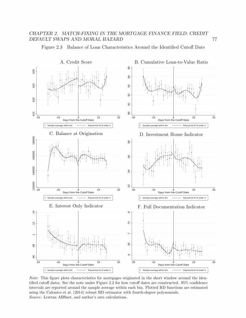
CHAPTER 2. MATCH-FIXING IN THE MORTGAGE FINANCE FIELD: CREDITDEFAULT SWAPS AND MORAL HAZARD 77
Figure 2.3 Balance of Loan Characteristics Around the Identified Cutoff Date
A. Credit Score
615
620
625
630
-20 -10 0 10 20Days from the Cutoff Date
Sample average within bin Polynomial fit of order 4
B. Cumulative Loan-to-Value Ratio
8081
8283
8485
-20 -10 0 10 20Days from the Cutoff Date
Sample average within bin Polynomial fit of order 4
C. Balance at Origination
1200
0014
0000
1600
0018
0000
-20 -10 0 10 20Days from the Cutoff Date
Sample average within bin Polynomial fit of order 4
D. Investment House Indicator
.02
.04
.06
.08
-20 -10 0 10 20Days from the Cutoff Date
Sample average within bin Polynomial fit of order 4
E. Interest Only Indicator
.06
.08
.1.1
2.1
4
-20 -10 0 10 20Days from the Cutoff Date
Sample average within bin Polynomial fit of order 4
F. Full Documentation Indicator
.6.6
5.7
.75
.8
-20 -10 0 10 20Days from the Cutoff Date
Sample average within bin Polynomial fit of order 4
Note: This figure plots characteristics for mortgages originated in the short window around the iden-tified cutoff dates. See the note under Figure 2.2 for how cutoff dates are constructed. 95% confidenceintervals are reported around the sample average within each bin. Plotted RD functions are estimatedusing the Calonico et al. (2014) robust RD estimator with fourth-degree polynomials.Source: Lewtan ABSnet, and author’s own calculations.

CHAPTER 2. MATCH-FIXING IN THE MORTGAGE FINANCE FIELD: CREDITDEFAULT SWAPS AND MORAL HAZARD 78
Figure 2.4 Effect of Cutoff Discontinuity on Prepayment Performance
A. Refinance
.1.1
2.1
4.1
6.1
8
-20 -10 0 10 20Days from the Cutoff Date
Sample average within bin Polynomial fit of order 4
B. Moving
.01
.02
.03
.04
.05
-20 -10 0 10 20Days from the Cutoff Date
Sample average within bin Polynomial fit of order 4
C. Pre-payoff
.05
.06
.07
.08
.09
.1
-20 -10 0 10 20Days from the Cutoff Date
Sample average within bin Polynomial fit of order 4
Note: This figure plots refinance, moving and pre-payoff performance for mortgages originated in theshort window around the identified cutoff dates. See the note under Figure 2.2 for how cutoff dates areconstructed. 95% confidence intervals are reported around the sample average within each bin. PlottedRD functions are estimated using the Calonico et al. (2014) robust RD estimator with fourth-degreepolynomials.Source: Lewtan ABSnet, and author’s own calculations.

CHAPTER 2. MATCH-FIXING IN THE MORTGAGE FINANCE FIELD: CREDITDEFAULT SWAPS AND MORAL HAZARD 79
Figure 2.5 Effect of Cutoff Discontinuity on Default Performance.3
.35
.4.4
5
-20 -10 0 10 20Days from the Cutoff Date
Sample average within bin Polynomial fit of order 4
Note: This figure plots default performance for mortgages originated in the short window aroundthe identified cutoff dates. See the note under Figure 2.2 for how cutoff dates are constructed. 95%confidence intervals are reported around the sample average within each bin. Plotted RD functions areestimated using the Calonico et al. (2014) robust RD estimator with fourth-degree polynomials.Source: Lewtan ABSnet, and author’s own calculations.

CHAPTER 2. MATCH-FIXING IN THE MORTGAGE FINANCE FIELD: CREDITDEFAULT SWAPS AND MORAL HAZARD 80
Tables
Table 2.1 Sample Descriptive Statistics
No CDSCovered
CDS Covered Total Obs
Panel A: Number of subprime Mortgages and Pools in the sample
Mortgages 5,189,001 2,934,787 8,123,788Pools 3,290 1,466 4,756
Panel B: Borrower and loan characteristics
Loan amt. 179,963 176,069 178,556 8,123,771Securitized amt. 178,373 174,836 177,122 7,023,087Credit Score 628.20 617.96 624.56 7,710,408CLTV(%) 83.52 81.61 82.84 7,155,742PrepaymentPenalty
0.45 0.40 0.44 6,044,016
Balloon Payment 0.15 0.05 0.11 8,123,788ARM 0.64 0.71 0.66 8,123,788Interest Only 0.13 0.12 0.12 7,869,502First Lien 0.83 0.85 0.84 8,123,788Investment House 0.06 0.04 0.06 7,554,674Full Documtation 0.54 0.54 0.54 7,614,619
Note: This table summarizes the characteristics of the subprime mortgages in the data sample. All thesubprime mortgages are originated during 2003–2007. A mortgage is defined to be covered by CDS ifat least one of the bonds or tranches that the mortgage pool is backing is referenced by CDS. Column(1) and (2) report the characteristics for non-CDS-covered and CDS-covered subsamples respectively.Column (3) reports the average characteristics for the full sample, and column (4) reports the totalnumber of observation.Source: Lewtan ABSnet and ATTOM.

CHAPTER 2. MATCH-FIXING IN THE MORTGAGE FINANCE FIELD: CREDITDEFAULT SWAPS AND MORAL HAZARD 81
Table 2.2 CDS Coverage Effect on Mortgage Prepayment
OLS Logit
(1) (2) (3) (4) (5)
CDS0.054∗∗∗ 0.054∗∗∗ 0.055∗∗∗ 0.042∗∗∗ 0.038∗∗∗
(0.008) (0.008) (0.007) (0.006) (0.007)
Controls X X X X XOri Year FE X XCBSA FE XOri Year ×CBSA FE
X X X
Servicer FE X XCluster Mort. Pool Mort. Pool Mort. Pool Mort. Pool Mort. PoolObservations 4,323,566 4,250,635 4,250,635 4,192,057 4,192,057
Note: This table reports the effect of CDS coverage effect on mortgage prepayment, obtained fromestimating equation (2.1). The controlled borrower and loan characteristics varibles include CLTV,credit score, Loan purpose, as well as prepayment penalty, interest only, balloon payment, ARM, firstlien, investment house and full documentation indicators. Column (1) controls observed borrowerand loan characteristics and origination year fixed effect. To match geographical distribution of themortgages, column (2) further includes core-based statistical area (CBSA) fixed effect. Column (3),instead, includes Ori Year × CBSA fixed effect to compare mortgages only originated in the same yearand located in the same CBSA. I control servicer fixed effect in specification (4) and resort to a logitmodel in specification (5). All observations are weighted by securitized amount of the loan. Standarderrors in parentheses are clustered at the mortgage pool level. ∗ p < 0.10, ∗∗ p < 0.05, ∗∗∗ p < 0.01. Incolumn (5), marginal effect of CDS coverage is reported.Source: Lewtan ABSnet, and author’s own calculations.

CHAPTER 2. MATCH-FIXING IN THE MORTGAGE FINANCE FIELD: CREDITDEFAULT SWAPS AND MORAL HAZARD 82
Table 2.3 CDS Coverage Prepayment Effect Breakdown
Refinance Moving Pre-Payoff
OLS Logit OLS Logit OLS Logit(1) (2) (3) (4) (5) (6)
CDS 0.036∗∗∗ 0.036∗∗∗ 0.002∗ 0.002 0.003 0.003(0.005) (0.007) (0.001) (0.002) (0.002) (0.002)
Controls X X X X X XOri Year ×CBSA FE
X X X X X X
Servicer FE X X X X X X
ClusterMort.Pool
Mort.Pool
Mort.Pool
Mort.Pool
Mort.Pool
Mort.Pool
Obs. 3,369,571 3,369,571 3,369,571 3,369,571 3,369,571 3,369,571
Note: This table reports the effect of CDS coverage effect on various types of mortgage prepayment:refinance, moving and payoff, obtained from estimating equation (2.1). All regressions control borrowerand loan characteristics include CLTV, credit score, Loan purpose, as well as prepayment penalty,interest only, balloon payment, ARM, first lien, investment house and full documentation indicators.Also all regressions control origination year by core-based statistical area (CBSA) fixed effect andservicer fixed effect. For each outcomes, I apply both the linear probability model and logit model.All observations are weighted by securitized amount of the loan. Standard errors in parentheses areclustered at the mortgage pool level. ∗ p < 0.10, ∗∗ p < 0.05, ∗∗∗ p < 0.01. In column (5), marginaleffect of CDS coverage is reported.Source: Lewtan ABSnet, ATTOM, and author’s own calculations.

CHAPTER 2. MATCH-FIXING IN THE MORTGAGE FINANCE FIELD: CREDITDEFAULT SWAPS AND MORAL HAZARD 83
Table 2.4 CDS Coverage Effect on Mortgage Refinance
OLS Logit
(1) (2) (3) (4) (5)
CDS0.061∗∗∗ 0.059∗∗∗ 0.058∗∗∗ 0.036∗∗∗ 0.036∗∗∗
(0.007) (0.007) (0.006) (0.005) (0.007)
Controls X X X X XOri Year FE X XCBSA FE XOri Year ×CBSA FE
X X X
Servicer FE X XCluster Mort. Pool Mort. Pool Mort. Pool Mort. Pool Mort. PoolObservations 3,437,007 3,406,643 3,406,643 3,369,571 3,369,571
Note: This table reports the effect of CDS coverage effect on mortgage refinance, obtained fromestimating equation (2.1). The controlled borrower and loan characteristics varibles include CLTV,credit score, Loan purpose, as well as prepayment penalty, interest only, balloon payment, ARM, firstlien, investment house and full documentation indicators. Column (1) controls observed borrowerand loan characteristics and origination year fixed effect. To match geographical distribution of themortgages, column (2) further includes core-based statistical area (CBSA) fixed effect. Column (3),instead, includes Ori Year × CBSA fixed effect to compare mortgages only originated in the same yearand located in the same CBSA. I control servicer fixed effect in specification (4) and resort to a logitmodel in specification (5). All observations are weighted by securitized amount of the loan. Standarderrors in parentheses are clustered at the mortgage pool level. ∗ p < 0.10, ∗∗ p < 0.05, ∗∗∗ p < 0.01. Incolumn (5), marginal effect of CDS coverage is reported.Source: Lewtan ABSnet, and author’s own calculations.

CHAPTER 2. MATCH-FIXING IN THE MORTGAGE FINANCE FIELD: CREDITDEFAULT SWAPS AND MORAL HAZARD 84
Table 2.5 CDS Coverage Effect on Mortgage Default
OLS Logit
(1) (2) (3) (4) (5)
CDS-0.022∗∗∗ -0.020∗∗∗ -0.022∗∗∗ -0.021∗∗∗ -0.018∗∗∗
(0.005) (0.005) (0.004) (0.004) (0.004)
Controls X X X X XOri Year FE X XCBSA FE XOri Year ×CBSA FE
X X X
Servicer FE X XCluster Mort. Pool Mort. Pool Mort. Pool Mort. Pool Mort. PoolObservations 4,323,566 4,250,635 4,250,635 4,192,057 4,191,070
Note: This table reports the effect of CDS coverage effect on mortgage default, obtained from esti-mating equation (2.1). The controlled borrower and loan characteristics varibles include CLTV, creditscore, Loan purpose, as well as prepayment penalty, interest only, balloon payment, ARM, first lien,investment house and full documentation indicators. Column (1) controls observed borrower and loancharacteristics and origination year fixed effect. To match geographical distribution of the mortgages,column (2) further includes core-based statistical area (CBSA) fixed effect. Column (3), instead, in-cludes Ori Year × CBSA fixed effect to compare mortgages only originated in the same year andlocated in the same CBSA. I control servicer fixed effect in specification (4) and resort to a logit modelin specification (5). All observations are weighted by securitized amount of the loan. Standard errorsin parentheses are clustered at the mortgage pool level. ∗ p < 0.10, ∗∗ p < 0.05, ∗∗∗ p < 0.01. Incolumn (5), marginal effect of CDS coverage is reported.Source: Lewtan ABSnet, and author’s own calculations.

CHAPTER 2. MATCH-FIXING IN THE MORTGAGE FINANCE FIELD: CREDITDEFAULT SWAPS AND MORAL HAZARD 85
Table 2.6 Summary Statistics for Local Randomization Sample
Percentile
MeanStd.Dev.
25th 50th 75th Obs.
A. Loan and Borrower Characterisitics
Loan amt. 164,899 126,985 80,800 130,500 212,000 26,372
Securitized amt. 167,639 124,758 83,378 131,781 211,887 25,137
Credit Score 626.48 59.14 585 624 664 26,271
CLTV(%) 82.19 12.95 79 80 90 25,987
Prepayment Penalty 0.50 0.50 0 1 1 15,968
Balloon Payment 0.10 0.30 0 0 0 26,372
ARM 0.56 0.50 0 1 1 26,372
Interest Only 0.09 0.28 0 0 0 26,329
First Lien 0.94 0.24 1 1 1 26,372
Investment House 0.05 0.23 0 0 0 25,422
Full Documtation 0.61 0.49 0 1 1 26,372
B. Ex Post Loan Performance Measures
Prepayment 0.36 0.48 0 0 1 26,372
Refinance 0.14 0.35 0 0 0 26,372
Moving 0.03 0.18 0 0 0 26,372
Pre-Payoff 0.08 0.26 0 0 0 26,372
Default 0.38 0.49 0 0 1 26,372
Note: This table reports summary statistics for the mortgages in the identified local randomizationsample (the set of loans originated within 5 days of one of the detected cutoff dates) used in estimation.Panel A reports loan and borrower characteristics. Panel B summarizes the outcome variables, includingprepayment (refinance, moving, pre-payoff) and default.Source: Lewtan ABSnet, ATTOM, and author’s own calculations.
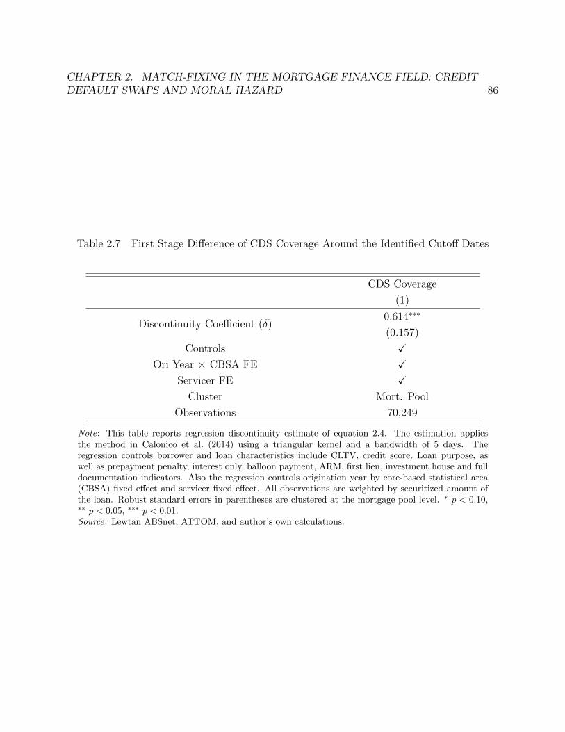
CHAPTER 2. MATCH-FIXING IN THE MORTGAGE FINANCE FIELD: CREDITDEFAULT SWAPS AND MORAL HAZARD 86
Table 2.7 First Stage Difference of CDS Coverage Around the Identified Cutoff Dates
CDS Coverage
(1)
Discontinuity Coefficient (δ)0.614∗∗∗
(0.157)
Controls X
Ori Year × CBSA FE X
Servicer FE X
Cluster Mort. Pool
Observations 70,249
Note: This table reports regression discontinuity estimate of equation 2.4. The estimation appliesthe method in Calonico et al. (2014) using a triangular kernel and a bandwidth of 5 days. Theregression controls borrower and loan characteristics include CLTV, credit score, Loan purpose, aswell as prepayment penalty, interest only, balloon payment, ARM, first lien, investment house and fulldocumentation indicators. Also the regression controls origination year by core-based statistical area(CBSA) fixed effect and servicer fixed effect. All observations are weighted by securitized amount ofthe loan. Robust standard errors in parentheses are clustered at the mortgage pool level. ∗ p < 0.10,∗∗ p < 0.05, ∗∗∗ p < 0.01.Source: Lewtan ABSnet, ATTOM, and author’s own calculations.

CHAPTER 2. MATCH-FIXING IN THE MORTGAGE FINANCE FIELD: CREDITDEFAULT SWAPS AND MORAL HAZARD 87
Table 2.8 Loan Characteristic Balance Regressions
CreditScore CLTV(%)
LoanAmount
Invest-mentHouse
InterestOnly
FullDocum-tation
(1) (2) (3) (4) (5) (6)
Discontinuity Coeff.-5.976 0.446 153 -0.006 -0.004 0.021
(3.579) (0.867) (8946) (0.019) (0.020) (0.025)
Controls X X X X X X
Ori Year × CBSA FE X X X X X X
Servicer FE X X X X X X
ClusterMort.Pool
Mort.Pool
Mort.Pool
Mort.Pool
Mort.Pool
Mort.Pool
Observations 70,249 70,044 68,646 70,249 68,402 70,131
Note: This table reports regression discontinuity estimate using equation 2.4. The estimation appliesthe method in Calonico et al. (2014) using a triangular kernel and a bandwidth of 5 days. Theregressions control borrower and loan characteristics as in Table 2.7 excluding the dependent variables.Also the regressions control origination year by core-based statistical area (CBSA) fixed effect andservicer fixed effect. All observations are weighted by securitized amount of the loan. Robust standarderrors in parentheses are clustered at the mortgage pool level. ∗ p < 0.10, ∗∗ p < 0.05, ∗∗∗ p < 0.01.Source: Lewtan ABSnet, ATTOM, and author’s own calculations.

CHAPTER 2. MATCH-FIXING IN THE MORTGAGE FINANCE FIELD: CREDITDEFAULT SWAPS AND MORAL HAZARD 88
Table 2.9 Loan Characteristic Balance Regressions
Refinance Moving Pre-Payoff
R.F. 2SLS R.F. 2SLS R.F. 2SLS
(1) (2) (3) (4) (5) (6)
Discontinuity Coeff.0.049∗∗ 0.005 0.024∗∗∗
(0.022) (0.006) (0.007)
CDS0.080∗∗ 0.008 0.039∗∗∗
(0.038) (0.009) (0.014)
Controls X X X X X X
Ori Year × CBSA FE X X X X X X
Servicer FE X X X X X X
ClusterMort.Pool
Mort.Pool
Mort.Pool
Mort.Pool
Mort.Pool
Mort.Pool
Observations 70,249 70,249 70,249 70,249 70,249 70,249
Note: This table reports regression discontinuity estimate of mortgage prepayment performance. Theoutcome variables are indicators for refinance, moving or pre-payoff. Column (1), (3) and (5) reportthe reduced form estimates directly obtaining from Equation 2.4. Column (2), (4) and (6) report the2-stage least square estimates of the effect of CDS coverage. The estimation applies the method inCalonico et al. (2014) using a triangular kernel and a bandwidth of 5 days. The regressions controlborrower and loan characteristics as in Table 2.7 excluding the dependent variables. Also the regressionscontrol origination year by core-based statistical area (CBSA) fixed effect and servicer fixed effect. Allobservations are weighted by securitized amount of the loan. Robust standard errors in parenthesesare clustered at the mortgage pool level. ∗ p < 0.10, ∗∗ p < 0.05, ∗∗∗ p < 0.01.Source: Lewtan ABSnet, ATTOM, and author’s own calculations.

CHAPTER 2. MATCH-FIXING IN THE MORTGAGE FINANCE FIELD: CREDITDEFAULT SWAPS AND MORAL HAZARD 89
Table 2.10 Loan Characteristic Balance Regressions
Default
Reduced Form 2SLS
(1) (2)
Discontinuity Coeff.-0.045∗∗
(0.019)
CDS-0.074∗∗
(0.033)
Controls X X
Ori Year × CBSA FE X X
Servicer FE X X
Cluster Mort. Pool Mort. Pool
Observations 70,249 70,249
Note: This table reports regression discontinuity estimate of mortgage default performance. Theoutcome variable is an indicator for default. Column (1) reports the reduced form estimates directlyobtaining from Equation 2.4. Column (2) reports the 2-stage least square estimates of the effect ofCDS coverage. The estimation applies the method in Calonico et al. (2014) using a triangular kerneland a bandwidth of 5 days. The regressions control borrower and loan characteristics as in Table 2.7excluding the dependent variables. Also the regressions control origination year by core-based statisticalarea (CBSA) fixed effect and servicer fixed effect. All observations are weighted by securitized amountof the loan. Robust standard errors in parentheses are clustered at the mortgage pool level. ∗ p < 0.10,∗∗ p < 0.05, ∗∗∗ p < 0.01.Source: Lewtan ABSnet, ATTOM, and author’s own calculations.

CHAPTER 2. MATCH-FIXING IN THE MORTGAGE FINANCE FIELD: CREDITDEFAULT SWAPS AND MORAL HAZARD 90
Table 2.11 CDS Party-Servicer Affiliation Effect
Prepay Refinance Moving Pre-Payoff Default
(1) (2) (3) (4) (5)
CDS0.042∗∗∗ 0.035∗∗∗ 0.001∗ 0.004∗∗∗ -0.018∗∗∗
(0.006) (0.005) (0.001) (0.001) (0.004)
Servicer-CDS Seller0.114∗∗ 0.096∗∗∗ 0.026∗∗∗ 0.007 -0.044∗∗∗
(0.045) (0.035) (0.008) (0.011) (0.015)
Servicer-CDS Buyer-0.021 -0.007 -0.002 -0.005 -0.032(0.033) (0.026) (0.003) (0.004) (0.021)
Controls X X X X XOri Year × CBSA FE X X X X XServicer FE X X X X XCluster Mort. Pool Mort. Pool Mort. Pool Mort. Pool Mort. PoolObservations 4,192,057 3,369,571 3,369,571 3,369,571 4,191,880
Note: This table reports the interactive effect of CDS coverage with CDS sellers’ and buyers’ affiliationwith mortgage servicers, obtained from estimating equation (2.5). The outcome variables includedummy variables for mortgage prepay, various types of mortgage prepayment (refinance, moving andpre-payoff), and default. The CDS sellers (buyers) and mortage servicers affiliation is equal to oneif they are within the same financial holding company. All regressions control borrower and loancharacteristics include CLTV, credit score, Loan purpose, as well as prepayment penalty, interestonly, balloon payment, ARM, first lien, investment house and full documentation indicators. Also allregressions control origination year by core-based statistical area (CBSA) fixed effect and servicer fixedeffect. For each outcomes, I apply both the linear probability model and logit model. All observationsare weighted by securitized amount of the loan. Standard errors in parentheses are clustered at themortgage pool level. ∗ p < 0.10, ∗∗ p < 0.05, ∗∗∗ p < 0.01. In column (5), marginal effect of CDScoverage is reported.Source: Lewtan ABSnet, ATTOM, and author’s own calculations.

91
Chapter 3
Residential Investment and theBusiness Cycle
3.1 Introduction
Huge effort has been devoted to predict the business cycle both in the industry and academiccommunities, but the performance of such prediction is notoriously poor. Leamer (2007)first documents a very stable leading relationship between residential investment and thebusiness cycle, which provides a hope of market-timing. But to make the best use of thisleading relationship, we need to understand the underlying mechanism, which has not beenfully explored in the literature.
The leading relationship can be seen in the panel (a) of Figure 3.1. The ratio of residentialinvestment to GDP (the residential investment component, black solid line) well leads thebusiness cycle (defined by NBER, shaded area covering recessions) in the postwar period. Tomake this point more clear, I extract the one-year-period residential investment componentbefore the start of each recession into panel (b). For illustration convenience, I shift theend of each path to 0 so that each point on the path denotes the percentage differencefrom the level of the residential investment component at the start of the coming recession.Strikingly, in ten of the eleven postwar recessions, the residential investment component hadbeen signaling a decreasing momentum since almost one year before the economy began toturn down. The only exception is the early 2000s recession which is triggered by the dot-combubble. Similarly, I extract the paths in the one-year period before the end of each recession,which are illustrated in panel (c). For at least six out of the eleven times, recovery signalswere found in the residential investment component paths before the trough of the businesscycle.
Such a striking leading relationship with the business cycle is not found in other invest-ment classes, but unique to the construction sector. The red dash lines in Figure 3.1 depictthe historical dynamics of the ratio of non-residential investment to GDP (the business in-vestment component), and exhibit exactly the opposite pattern. The business investment

CHAPTER 3. RESIDENTIAL INVESTMENT AND THE BUSINESS CYCLE 92
component synchronizes better with the business cycle. It rises before the advent of eco-nomic downturn, and drops over the full course of the recession. Such “Residential Leading,Business Lagging” pattern is further demonstrated in the correlation structure shown inTable 3.1. Residential investment indicators have stronger positive correlation with the realGDP in the next year, while business investment indicators are more correlated with the oneyear lag of the real GDP.
Macroeconomists have tried to reproduce the stylized facts of the residential investment,including procycalicality, volatility and leading relationship, by adding one more construc-tion sector and housing consumption into the standard real business cycle (RBC) model(e.g. Davis and Heathcote (2005), Piazzesi and Schneider (2016) for a comprehensive sur-vey). While successfully reconciling the other patterns, such multi-sector models are notable to account for the “Residential Leading, Business Lagging” pattern, mostly becauseconstruction sector and other sectors are functionally symmetric. As a result, both resi-dential and business investment should react to exogenous demand or TFP shocks in thesame direction. Therefore, it is impossible to generate a diverging pattern of residential andbusiness investment before the advent of an economic peak or trough.
This paper aims to explain the “Residential Leading, Business Lagging” pattern by stress-ing the heterogeneity in the value storage technology between construction and manufactur-ing sectors. Residential investment is a technology that transforms perishable consumptiongoods into durable houses that deliver housing service in the future, while business investmentis to transform the same perishable consumption goods into production capital that couldgenerate more perishable consumption goods later. Production assets are highly specialized,and are exposed to large value reduction when the holding firm goes bankrupt (for example,due to capital displacement). Houses, however, do not suffer from such displacement losses,because the houses provide generic housing service, and hence are equally valuable to anyowner.
Therefore, the value stored in the form of production capital through business investmenttechnology is exposed to corporate bankruptcy risk, while that in the form of houses throughresidential investment technology does not. With such difference in mind, the representa-tive agent optimally allocates the resources between residential and business investment, inresponse to the time-varying corporate bankruptcy rate, as can be seen in Figure 3.2. Atthe period of economic booms, bankruptcy risk is low, so business investment is less risky.More of the value should be stored in the form of business investment, rather than residentialinvestment. As a result, we see a decreasing residential investment component and a risingbusiness investment share when the economy is running up.
Specifically, I introduce an exogenous corporate bankruptcy shock into a two-sector (man-ufacturing and construction) real business cycle (RBC) model, and assume that bankruptcybrings value destruction (economic inefficiency) on top of the physical depreciation to the liv-ing capital, while house structures only suffer from constant physical deprecation. When thebankruptcy rate is low (booms), the firm has little probability to suffer from huge bankruptcylosses. Hence it is optimal to invest more on the manufacturing sector, taking advantageof the low bankruptcy rate. Therefore, we observe the business investment component ris-

CHAPTER 3. RESIDENTIAL INVESTMENT AND THE BUSINESS CYCLE 93
ing, and the residential investment component decreasing before the advent of economicdownturn.
While the model in this paper takes the different value destruction features in the twostorage technologies as granted, it can be microfounded by the idea of capital specificity.Manufacturing capital is built for specific purposes. If the holding firm goes bankrupt,liquidating such specialized capital would incur economic inefficiency, since the capital haslower value in its second best use (Brunnermeier, Eisenbach, and Sannikov, 2012). Forexample, aerospace companies invest huge amount of money to build wind tunnels thatare able to produce winds as fast as 270 miles per hour. But when the companies areliquidated and sell these tunnels to other businesses such as bicycle helmet designers, atmost one third of the tunnel value can be recovered (Ramey and Shapiro, 2001). Sucheconomic inefficiency due to displacement is further amplified through two channels. Rameyand Shapiro (2001) propose that assets with higher specificity have higher searching costand hence, have higher probability of displacement. Shleifer and Vishny (1992) argue thatthe firms in the same industry are likely to be financially distressed at the same time due toindustry-wide adverse shocks. Therefore, when a firm goes bankrupt and tries to liquidateits specialized assets, the natural second-best users might not be able to afford the assets,which aggravates capital displacement and economic inefficiency. Empirically, Pulvino (1998)studies the airline industry, and shows such displacement cost can be as high as 30% of themarket price when liquidating aircraft during market recessions.
Residential structures, on the other hand, deteriorate constantly, and is not exposed todisplacement risk, because the function of the house is much more generic. Although we dosee mortgage defaults and very low recovery rate during the following foreclosure process,the economy does not necessarily incur inefficiency as long as there are buyers that fullyvalue the housing services filling in the houses soon. From social planner’s point of view,such “fire sale” is only a transfer of value from the left hand to the right.
In the spirit of the house filtering literature (Baer and Williamson, 1988), homeownervacancy rate is indicative of the social inefficiency of the housing utilization. From Figure3.2, we can see that historical homeowner vacancy rate is much less volatile than corporatedefault rate. It varies within the range from 1% to 2% before the recent crisis. In this paper,I assume the cost due to vacancy to be constant over time, and attribute such cost to thephysical deterioration of housing structures without loss of generality.
Literature review. This paper contributes to the real business cycle (RBC) literatureby explicitly including an exogenous bankruptcy shock. Different from classic RBC modelsthat assume the firms are long-lived, and recycle the capital after constant physical depre-ciation, this paper interprets the capital depreciation as the aggregate of constant physicaldepreciation and dynamic capital displacement losses due to corporate bankruptcy. Inclu-sion of such dynamic depreciation rate would enrich the bare-bone RBC model, as Amblerand Paquet (1994) do to reconcile the weak correlation between production and workinghours. Specifically, the bankruptcy shock triggers out the diverging behavior of the residen-tial investment and the business investment due to their different exposure to bankruptcy

CHAPTER 3. RESIDENTIAL INVESTMENT AND THE BUSINESS CYCLE 94
risk.The opposite reactions to the bankruptcy shock between the residential and business
investment are empirically verified in my vector autocorrelation analysis. With a mild iden-tification assumption that both residential and business investment do not react to thecontemporaneous bankruptcy shock, which is consistent with the empirical observation thatthe average time between investment decision and completion ranges from 6 months to 14months (Edge, 2000), I am able to identify the structural bankruptcy shock, and capture theimpulse responses to such a structure shock. When bankruptcy risk is lower than equilib-rium level, the residential investment component will dip down gradually with the businessinvestment component spiking up, which matches my model predictions. Most importantly,it provides empirical evidence that bankruptcy risk is a valid state variable to differentiatethe dynamics of residential investment from that of other investment classes.
Overview. In what follows, I set up a real business cycle model with two productionsectors in section 3.2. The simulated results from the theoretical model are shown in section3.3. Section 3.4 describes my empirical strategy, the data I used for testing, and the empiricalresults which coincide with my theoretical predictions. Section 3.5 compares the results fromboth theoretical part and empirical part, and section 3.6 concludes.
3.2 The Model
To formalize the idea, I introduce a stylized real business cycle model with multiple produc-tion sectors. Different from other multi-sector RBC models (Davis and Heathcote, 2005), Iintroduce a new bankruptcy shock, which is represented by a stochastic depreciation rateprocess in the model. Given constant physical depreciation rate, the aggregate depreciationrate can be seen as a sufficient statistic of bankruptcy losses. A key assumption of the modelis that such stochastic bankruptcy losses are incurred only on the production capital, but noton the housing stock.1Corporate bankruptcy triggers the displacement of the assets due totheir specificity, while houses do not incur such dead-weight losses for their generic function.
At this stage, I have made two more restrictions to the model for simplicity. First, themodel considered here abstracts labor supply away to highlight the interactions of the capitalinvestment and the bankruptcy risk. Alternatively, we can think that labor supply is fixedat its natural level. Second, the ex ante and ex post bankruptcy rates are equal. Thisassumption allows me to apply log-linearization technique to the problem.
A representative household with constant population growth rate log(η) rents homoge-neous capital Kt to perfectly competitive firms. These firms allocate the capital frictionlesslyacross two different sectors: manufacturing Kmt and construction Kht. The manufacturing
1In fact, this is an extreme case without any loss of generality. We can, alternatively, assume housingstructures suffer from displacement losses, but the risk exposure is lower than manufacturing capital. Theresult would be the same qualitatively.

CHAPTER 3. RESIDENTIAL INVESTMENT AND THE BUSINESS CYCLE 95
sector has the following production technology:
Ymt = AmtKαmmt (3.1)
Amt+1 = Aρmmte(1−ρm)(gAm+εmt+1) (3.2)
where the production shifter Amt represents a combination of labor supply and manufac-turing productivity. Since the labor supply per person is fixed in the model, the trend ofAmt is controlled by population growth as well as the manufacturing productivity long-runtrend, while the short-run dynamics of Amt reflects the short-run variation of manufacturingproductivity.
Similarly, the construction technology follows
Yht = AhtKαhht (3.3)
Aht+1 = Aρhht e(1−ρh)(gAh+εht+1) (3.4)
where the production shifter Aht represent a combination of construction labor supply, con-struction productivity and land supply. To simplify the interpretation, let us assume landsupply is also fixed, then the short-run dynamics of Aht just represent the short-run variationof construction productivity.
The perishable goods produced by the manufacturing sector have three uses. Ct amountwill be sold to households for consumption, Imt amount will be reinvested to build specializedcapital (e.g. wind tunnels) by manufacturing firms themselves, and Iht amount will be sold toconstruction firms for their investment. For example, construction firms need to buy cranes,excavators and trucks from manufactures. These construction investment would eventuallybe transformed into durable housing structures.
Ymt = Ct + Imt + Iht (3.5)
The capital in either of the sectors follows the following evolution process:
Kit+1 = (1− dtδk)Kit + Iit, i ∈ {m,h} (3.6)
where dtδk is the aggregate depreciation rate, which includes both physical depreciation andbankruptcy losses. As I have argued in the introduction, the bankruptcy of the holding firmwould bring a huge depreciation to the capital due to displacement of the specialized assets.Therefore, δk captures the historical mean of the physical depreciation plus bankruptcy losses,and dt captures its short run dynamics, which is modeled as a mean reversion process:
dt+1 = dρdt eεdt+1 (3.7)
where εt is a white noise, ρd captures the persistence of the exogenous shocks. Here I holdthe physical depreciation rate to be constant, so dt is a sufficient statistic of the bankruptcyrate. For this reason, I interchangeably use the depreciation shock and the bankruptcy shock

CHAPTER 3. RESIDENTIAL INVESTMENT AND THE BUSINESS CYCLE 96
to refer to dt thereafter. Noticeably, this exogenous bankruptcy shock is the key feature thatdistinguishes my framework from other RBC models in this line of literature.
For the construction sector, the newly constructed houses Yht will be added into thecurrent housing stock Ht, providing housing service to the households.
Ht+1 = (1− δh)Ht + Yht (3.8)
The housing stock also suffers from physical depreciation, but at a constant rate δh. Thehousing depreciation comes from the depreciation of housing structures, such as roof repairand drainage maintenance. I assume that the housing depreciation does not involve stochas-tic terms because the service of houses is much more generic than production machines andother manufacturing assets. Even if the house owner goes bankrupt, and has to foreclose hisor her house at a discounted price, displacement cost is not incurred as long as the house isas valuable to the buyer as to the seller.
The model is closed by the optimization problem of a representative household, whosefamily member derives utility from both consumption and housing stock.
Ut =
(cµt h
1−µt
)1−σ1− σ
(3.9)
From here forward, the letters in lower cases denote the amount per capita of the corre-sponding variables. The preference assumption is standard in macro and real estate litera-ture. The utility exhibits constant relative risk aversion toward the composite consumptionbundle, which combines non-durable consumption and housing stock in a Cobb-Douglas way.The intertemporal elasticity of substitution is 1/σ, and the non-durable consumption sharein the composite consumption bundle is µ.
The number of family members grows at the rate of log(η), and the discounting factor isdenoted by β. The household maximizes its expected utility of all family members.
maxct,ht
U =E∞∑t=0
(βη)t(cµt h
1−µt
)1−σ1− σ
Social Planner’s Problem
Since the firms are perfectly competitive, and there are no other market frictions, the FirstWelfare Theorem applies to this model. So we can equivalently solve the following social

CHAPTER 3. RESIDENTIAL INVESTMENT AND THE BUSINESS CYCLE 97
planner’s problem to achieve the model solution.
maxct,ht
U =E
[∞∑t=0
(βη)t(cµt h
1−µt
)1−σ1− σ
](3.10)
s.t. ct + ηkt+1 =(1− dtδk)kt + Amtkαmmt (3.11)
ηht+1 =(1− δh)ht + Aht(kt − kmt)αh (3.12)
dt+1 =dρdt eεdt+1 (3.13)
Amt+1 =Aρmmte(1−ρm)(gAm+εmt+1) (3.14)
Aht+1 =Aρhht e(1−ρh)(gAh+εht+1) (3.15)
As can be seen, the model has three exogenous shocks in total: two productivity shocks(εmt+1 and εht+1) and one bankruptcy shock (εdt+1). They can give us rich dynamics of themodeled economy. But for now, let us shut down the productivity shocks (εmt+1 = εht+1 = 0),and focus on the dynamics driven only by the bankruptcy shock. Then the productivity inboth sectors are deterministic trends, with growth rate gAm and gAh respectively.
The social planner does not have to concern either the trading between firms and house-holds, or the price of the production inputs and outputs. She just optimally allocates thecapital to the two sectors, and decides the policy of consuming and investing, based on therealized productivity and bankruptcy rate dynamics.
Detrending and Reparametrization
Since the two technologies have deterministic trends, all the other variables in this systemalso contain long-run trends, and thus are not stationary. Technically, it is much easier todeal with a stationary system. So the solution strategy is to first detrend each variable inthe original system, and then solve the detrended system.
Table 3.2 displays the balanced growth rate of each running variable per capita in themodel. Overall, the growth rates are determined by the productivity growth rate and thecapital share in the two sectors.
Then I detrend all the running variables by taking off their corresponding long termtreads:
st = e−gstst. (3.16)
Then the hatted variables are all stationary, and the social planner’s problem can be trans-

CHAPTER 3. RESIDENTIAL INVESTMENT AND THE BUSINESS CYCLE 98
formed into a stationary system:
maxct,ht
U =E∞∑t=0
βt
(cµt h
1−µt
)1−σ1− σ
(3.17)
s.t. ct + η1kt+1 =(1− dtδk)kt + Amkαmmt (3.18)
η2ht+1 =(1− δh)ht + Ah(kt − kmt)αh (3.19)
dt+1 =dρdt eεdt (3.20)
with reparametrization
β =βη exp
{µ+ (1− µ)αh
1− αmgAm + (1− µ)gAh
}(3.21)
η1 =η exp
{1
1− αmgAm
}(3.22)
η2 =η exp
{αh
1− αmgAm + gAh
}(3.23)
Am =Am,0 (3.24)
Ah =Ah,0 (3.25)
Since I shut down the short-run variation of the two productivity shocks, the detrendedproductivity of both sectors are degenerated into two constants, Am and Ah.
3.3 Model Results
The model solution is included in the technical note A.4. Before we jump into the solutionand the simulated results of the model, we can anticipate some key properties in this simplesetting. The social planner has two types of storage technologies to save perishable goods.One is to transform these perishable goods into manufacturing capital, and the other is totransform them into houses. Both storage technologies could yield utility to the representa-tive agents every period. The key difference between these two technologies is that the valueof manufacturing capital is controlled by the volatile bankruptcy dynamics, while the valueof housing structures is free from the bankruptcy risk. As a result, the social planner wouldoptimally allocate the investment between the manufacturing and construction sectors inresponse to the time-varying bankruptcy risk. When the economy is running well, corporatebankruptcy rate is low. It is optimal to increase the share of business investment and de-crease the share of residential investment. This pattern will be seen in the model simulationbelow.

CHAPTER 3. RESIDENTIAL INVESTMENT AND THE BUSINESS CYCLE 99
Parameters
To simulate the model, we first need to feed the system with appropriate parameters. Table3.3 summarizes the parameter values I use for the simulation. The time unit of the model is1 year, so the parameter values are on the annual basis.
The nondurable good share is set to 61% in the composite consumption bundle, so that thesteady state level of residential investment component matches its historical mean. Relativerisk aversion coefficient is 2, and discounting factor is 0.95, which are widely used in the RBCliterature (Davis and Heathcote, 2005). The historical mean of aggregate depreciation rate is6.5% every year, which is the sum of the annual manufacturing depreciation rate estimatedby Bureau of Economic Analysis, and the historical average of the corporate default ratepublished by Moody’s. The depreciation rate of residential structures is 1.4%, estimated byBureau of Economic Analysis. Capital production share in the manufacturing sector is 31%,much higher than that in the construction sector (13.2%). Technology is developing at anannual rate of 1.86% in the production sector, and 0.81% in the construction sector. All thecapital share and technology trend parameters are estimated by NIPA data. Population isgrowing at a rate of 1.67% per year, and the average rate of growth of hours worked in theprivate sector in the postwar period. The bankruptcy shock is highly persistent with thefirst order autocorrelation of 0.9. For the moment, I just set Ac,0 and Ah,0 to be 1, becausetheir values do not affect the impulse response functions of the detrending system.
Impulse Response Functions
With the parameter values listed above, I can fully solve the log-linearized model. Toillustrate how the system, especially residential investment and business investment, reactsto the bankruptcy shock, I plot the impulse response functions as shown in Figure 3.3.
First, we can notice from the impulse response of aggregate depreciation rate that, theeffect of bankruptcy shock is rather persistent. The half life is about 5 years.
If the economy is hit by one unit of negative bankruptcy shock, after a period of economicbooms, the aggregate depreciation rate is low due to lower bankruptcy rate. The firmwould first increase its investment in the manufacturing sector, taking advantage of very lowdepreciation rate right after the shock, as shown in the middle panel of Figure 3.3.
If we look closely on the impulse response of the business investment, it starts from 0since it takes one period for capital to adjust for the exogenous depreciation shock. It isconsistent with the fact that the average time between investment decision and completionranges from 6 months to 14 months (Edge, 2000). Then the business investment will risefirst, and then decrease down below 0. Since the economy expects aggregate depreciation iscoming back to its equilibrium level slowly, it is optimal for the firms to frontload investment,taking advantage of very low depreciation rate right after the shock. After a few years, thefirms have accumulated enough capital, and begin to reduce their capital investment.
The residential investment share is defined as the value of residential investment (newhousing structures) over the value of overall capital investment. It corresponds to the res-

CHAPTER 3. RESIDENTIAL INVESTMENT AND THE BUSINESS CYCLE 100
idential share of aggregate investment used in the following VAR analysis. Since I directlysolve the social planner’s problem to achieve the solutions. Price level of new houses does notshow up in the solution part. But we can easily set up firms’ profit maximization problemfor the two sectors, and get the price level from the first order conditions.
The impulse response of the residential investment share exhibits the opposite patternfrom that of the business investment. When the economy is running well, the bankruptcyrate goes down. Residential investment decreases initially since the economy optimally shiftsmore resource to the business side, taking advantage of the high level of sustainability ofmanufacturing capital. After a few years when the aggregate depreciation rate recovers closerto its equilibrium level, more and more resource is moved away from the manufacturingsector, back to the construction sector. Thus, we see a “check” curve of the residentialinvestment share.
3.4 Empirical Testing
To examine the fitness of my model with the data, I employ the Vector AutoRegression (VAR)model to estimate the response of the residential investment and the business investment tobankruptcy shocks. The VAR representation can be written as: rt
itdt
= Φ(L)
rtitdt
+
erteitedt
where rt denotes the ratio of residential investment to aggregate investment, it represents realbusiness investment, and dt is a bankruptcy rate variable, which captures the full dynamicsof aggregate depreciation rate. The time trend of all the 3 variables are removed. et are thereduced-form residuals, which are linear combinations of the exogenous shocks: ert
eitedt
=
a11 a12 0a21 a22 0a31 a32 a33
εrtεitεdt
In such a VAR specification, I have maintained most characteristics from the model. The
dimension of state variables are kept to be 3, as required by the model. The bankruptcyshock does not have instant effect on the contemporary investment both on the residentialand business side. It is consistent with the fact that the average time between investmentdecision and completion ranges from 6 months to 14 months (Edge, 2000). This is the keycondition to my identification strategy.
There are also differences between the model and the empirical framework. The modelregards bankruptcy shock as the only exogenous shock (εrt = εit = 0), and the bankruptcyrate, therefore, does not react to any other shocks (a31 = a32 = 0), while the VAR specifica-tion allows more flexibility. The stylized model focuses on illustrating the most striking facts

CHAPTER 3. RESIDENTIAL INVESTMENT AND THE BUSINESS CYCLE 101
that are only motivated by bankruptcy concerns. The data, however, contain much morecomplex economic components and noises. Therefore, we need a more flexible specificationto accommodate the data. But the inclusion of two more shocks brings up a new question:how we can disentangle the bankruptcy shock from the other shocks. Now let me discussmy identification strategy.
Identification Strategy
Cholesky Decomposition is widely used to identify structure shocks in VAR systems. Toapply Cholesky Decomposition, we need to make sure that the structure shocks are indeedlower-triangularly arranged. If a12 = 0, the transformation matrix is then lower-triangular,Cholesky decomposition applies naturally.
In our case, however, it is not realistic to argue that overall investment decisions do notaffect the residential investment share contemporaneously. In fact, such two investment-levelindicators are often simultaneously driven by some other shocks, such as monetary policy,and hence are very likely to be interdependent.
Fortunately, strictly lower-triangularity is not a necessary condition to identify the bankruptcyshock through Cholesky Decomposition. As an application of Keating (1996), Cholesky De-composition is able to correctly identify the bankruptcy shock as long as the transformationmatrix is block lower-triangular, which is the case in my VAR specification.
Specifically, the existence of a12 does affect the identification of the residential investmentshock εrt and the business investment shock εit, but the bankruptcy shock εdt can still beidentified due to the block recursiveness of the structural matrix. And the bankruptcy shockis what we really care about.
Data Description
All the time series used in this paper are annual data, and the range is from 1948 to 2010.All the macro variables except for default rate are from national income and product ac-counts (NIPA). Specifically, the nominal residential investment is directly taken from NIPAtable 1.1.5, while the nominal business investment aggregates different pieces including totalprivate business investment, gross federal non-defense investment and state and local grossinvestment. Real terms of corresponding variables use chained-dollar value whenever theyare available from NIPA, as the advantage of such statistic method is widely accepted andstressed by Landefeld, Moulton, and Vojtech (2003).
The ex post bankruptcy rate is hard to estimate, especially at the aggregate level. I useannual default rate punished by Moody’s (Emery, Ou, Tennant, Kim, and Cantor, 1920)as a proxy for bankruptcy rate, by assuming ex ante and ex post bankruptcy rates are thesame. Although Moody’s focuses on the firms with long-term debt issuance, the default rateis still highly correlated with economy-wide operation status of firms, and acts as my bestguess.

CHAPTER 3. RESIDENTIAL INVESTMENT AND THE BUSINESS CYCLE 102
In the VAR system, the variable rt is constructed by detrending the ratio of the residentialinvestment to the aggregate investment, and it is detrended log real business investment.Such choice corresponds to the simulated impulse response function in Figure 3.3. Alternativechoice of variables will be tested in the robustness part.
Empirical Results
I first estimate the VAR representation with the Matlab routines. Bayesian InformationCriterion (BIC) chooses 1 as the maximal lag number. Then I apply Cholesky Decompositionto disentangle the default rate shock (D shock) from the VAR residuals. As argued in theIdentification Strategy part, Cholesky Decomposition is sufficient to identify the D shockunder my structural assumption and ordering of rt, it and dt.
Figure 3.4 depicts the empirical counterpart of the simulated impulse response functionsin Figure 3.3 under my VAR specification. The confidence intervals are constructed bybootstrapping the implied VAR residuals 2000 times, and are delimited at 90% confidencelevel.
Overall, the empirical impulse response functions follow the same pattern as the simulatedones. The default rate decays geometrically as the aggregate depreciation rate in the model.When default rate is below its balanced path, business investment will bounce up from thenext period onward, though the instant response is forced to be zero. As analyzed in themodel part, in the first few periods, the firms would “over-invest” to take advantage of thelow default rate. When they feel that enough capital has been accumulated, the pace ofinvestment would slow down, and come back to its equilibrium level. As indicated by the90% confidence interval, such effect is statistically significant.
On the residential side, the effect is the opposite. When the default rate is low, moreof the resources would be devoted to the manufacturing sector. So the residential share ofthe investment would drop from 0 to below. The point estimate of the response in the firstfew years ranges from 1% to 1.5%, which means that if the default rate drops by 1%, theresidential share of the investment for the next year would decrease by 1% to 1.5%, stay atthat level for a few more years, and then slowly come back. Again, the effect is statisticallysignificant.
Robustness
As implied by the model, any three running variables would be sufficient to span the statevariable space, and fully capture the dynamics of the economy. When we try to explore thepattern of the data, the model seems too skinny. The choice of state variables are actuallyimportant to the key results of this paper. To avoid the concern of data mining, I illustratehere the results from an alternative choice of state variables.
In the VAR specification above, the second variable is detrended log real business invest-ment, which has a totally different denomination from the other two percentage series. So weshould also try to include percentage data to represent the dynamics of business investment.

CHAPTER 3. RESIDENTIAL INVESTMENT AND THE BUSINESS CYCLE 103
The business share of aggregate investment first comes to our mind, but does not work, sinceit is perfectly negatively correlated with residential share. My choice here is the businessinvestment component of GDP.
I rerun the above estimation and decomposition, and depict the impulse response func-tions to the identified D shock in figure (3.5). The pattern of the responses squares almostperfectly with the pattern I have shown above. Notably, the point estimation of the firstperiod impulse response of business investment share is 0.2, which means that if the defaultrate drops by 1%, the business investment share of the aggregate output for the next yearwould increase by about 0.2%.
3.5 Discussion
It is exciting to see that the impulse response pattern implied by my model echoes in itsempirical counterpart. But there is still some mismatch between them.
First, although the initial empirical response of the business investment matches themodel, it slowly comes back to its initial level. The model, on the other hand, has differentimplication, that investment would dip down below its equilibrium level, and then recovers.Such model pattern results from a dynamic optimization choice when firms face a long-livedrising aggregate depreciation rate. The firms frontload large amount of investment to takeadvantage of the low depreciation rate. The followed underinvestment is unavoidable becausethe shock itself reduces the depreciation of the production capital, and that is the first-ordereffect. The same problem applies to the response of the residential investment.
To solve such problems, we should shock the economy in a different way. To be spe-cific, the shock itself should not have first order effect. For example, the shock might be adecrease of ex ante bankruptcy volatility, or the decrease of the bankruptcy tail risk, whilethe expectation of bankruptcy rate remains the same. For risk aversion incentives, the firmshould also increase their business investment, and reduce new construction of houses. Atechnical difficulty of such model is that we cannot use log-linearization any more, since log-linearization first shuts down all the randomness, and only solves the first-order problem. Afull characterization of the solution dynamics is needed to conduct such experiments in thehigher order. I will further invest more in such models.
Second, we really need highly persistent bankruptcy rate to have the right impulse re-sponse functions. However, the persistence of the default rate is smaller than that I use inthe simulated data. But this can be jointly solved with the first problem.
3.6 Conclusion
I introduce a new state variable, bankruptcy rate, to explain the stylized fact, that residentialinvestment drops before the advent of economic downturn and recovers earlier than therecession ends. After the period of economic booms, the bankruptcy rate is low, and the

CHAPTER 3. RESIDENTIAL INVESTMENT AND THE BUSINESS CYCLE 104
business investment is expected to suffer from low level of bankruptcy losses. As a result,more of the resource would be shifted away from the residential side, where there is littlebankruptcy concern. Thus, we see a decreasing residential investment share of aggregateoutput, and an increasing business investment share. Whether such over-investment in thebusiness side contributes to the crisis, is out of my model, but definitely worth investigatingfurther.
This paper picks up a key difference between the residential and business investment, thatthe residential investment is subject to smooth depreciation, while the business investmentis exposed to volatile depreciation due to bankruptcy and asset displacement.

CHAPTER 3. RESIDENTIAL INVESTMENT AND THE BUSINESS CYCLE 105
Figures
Figure 3.1 Residential Investment Leads the Business Cycle
Q1-50 Q1-60 Q1-70 Q1-80 Q1-90 Q1-00 Q1-102
3
4
5
6
7
8
Per
cent
age
of R
esid
entia
lIn
vest
men
t in
GD
P
10
12
14
16
18
20
Per
cent
age
of B
usin
ess
Inve
stm
ent i
n G
DP
Residential Investment/GDPBusiness Investment/GDP
Panel (a) Historical Paths Of Residential And Business Investment
Q1-50 Q1-60 Q1-70 Q1-80 Q1-90 Q1-00 Q1-10
-0.5
0
0.5
1
1.5
Per
cent
age
Diff
eren
ce fr
om th
e le
vel
at th
e st
art o
f the
com
ing
Rec
essi
on
Residential Investment/GDPBusiness Investment/GDP
Panel (b) The Paths During The One Year Before The Start Of Each Recession

CHAPTER 3. RESIDENTIAL INVESTMENT AND THE BUSINESS CYCLE 106
Q1-50 Q1-60 Q1-70 Q1-80 Q1-90 Q1-00 Q1-10
-1
-0.5
0
0.5
1
1.5
Per
cent
age
Diff
eren
ce fr
om th
e le
vel
at th
e en
d of
the
Rec
essi
on
Residential Investment/GDPBusiness Investment/GDP
Panel (c) The Paths During The One Year Before The End Of Each Recession
Note: The data are quarterly. The shaded areas are NBER-designated recessions. Panel (b) depictsthe paths of residential investment/GDP (black solid) and business investment/GDP (red dash) duringthe one-year period before the start of each recession. The end of each path is shifted to 0 so that eachpoint on the path denotes the percentage difference from the corresponding level at the start of thecoming recession. Panel (c) depicts the paths during the one year before the end of each recession.Source: NIPA and author’s own calculations.

CHAPTER 3. RESIDENTIAL INVESTMENT AND THE BUSINESS CYCLE 107
Figure 3.2 Historical Dynamics of Corporate Default Rate
Q1-50 Q1-60 Q1-70 Q1-80 Q1-90 Q1-00 Q1-100
1
2
3
4
5
6
Per
cent
age
Corporate Default RateHomeowner Vacancy Rate
Note: The time series are annual. The corporate default rate is from Moody’s, and the homeownervacancy rate is from US. Bureau of the Census. The shaded areas are NBER-designated recessions.Source: Moody’s and US. Bureau of the Census.

CHAPTER 3. RESIDENTIAL INVESTMENT AND THE BUSINESS CYCLE 108
Figure 3.3 Impulse Response to One Unit Negative Bankruptcy Shock (Simulated)
0 2 4 6 8 10-0.2
-0.1
0
0.1
0.2
0.3
0.4Residential Investment Share
0 2 4 6 8 10-0.1
-0.05
0
0.05
0.1
0.15Business Investment
0 5 10-1
-0.5
0Aggregate Depreciation
Note: The three impulse responses are simulated using the model in section 3.2 with parameters inTable 3.3. The shock is one unit of negative bankruptcy shock. The horizon is 10 years after theeconomy is hit by the negative bankruptcy shock. The residential investment share is defined as thevalue of residential investment (new housing structures) over the value of overall capital investment.Source: Author’s own calculations.

CHAPTER 3. RESIDENTIAL INVESTMENT AND THE BUSINESS CYCLE 109
Figure 3.4 Impulse Response to One Unit Negative Default Shock (VAR)
0 5 10-3
-2
-1
0
1
Resonse of rt to 1 unit D shock
Order: rt, i
t, d
t
90% CI (2000 Bootstrap)
0 5 10-0.2
0
0.2
0.4
0.6
Resonse of it to 1 unit D shock
Order: rt, i
t, d
t
90% CI (2000 Bootstrap)
0 5 10-1
-0.5
0
0.5
Resonse of dt to 1 unit D shock
Order: rt, i
t, d
t
90% CI (2000 Bootstrap)
Note: The three impulse responses are estimated through the VAR framework in section 3.4. rt denotesthe ratio of residential investment to aggregate investment, it represents real business investment, anddt is a bankruptcy rate variable, which captures the full dynamics of aggregate depreciation rate. Thehorizon is 10 years after the economy is hit by the negative bankruptcy shock. The confidence intervalsare constructed by bootstrapping the implied VAR residuals 2000 times, and are delimited at 90%confidence level. Bayesian Information Criterion (BIC) chooses 1 as the maximal lag number.Source: NIPA, Moody’s and author’s own calculations.

CHAPTER 3. RESIDENTIAL INVESTMENT AND THE BUSINESS CYCLE 110
Figure 3.5 Impulse Response to One Unit Negative Default Shock (Alternative VAR)
0 5 10-3
-2
-1
0
1
Resonse of rt to 1 unit D shock
Order: rt, i
t, d
t
90% CI (2000 Bootstrap)
0 5 10-1
0
1
2
3
4
Resonse of it to 1 unit D shock
Order: rt, i
t, d
t
90% CI (2000 Bootstrap)
0 5 10-1
-0.5
0
0.5
Resonse of dt to 1 unit D shock
Order: rt, i
t, d
t
90% CI (2000 Bootstrap)
Note: The three impulse responses are estimated through the alternative VAR specification by refiningit. rt denotes the ratio of residential investment to aggregate investment, it represents the ratio ofbusiness investment to aggregate investment, and dt is a bankruptcy rate variable, which captures thefull dynamics of aggregate depreciation rate. The horizon is 10 years after the economy is hit by thenegative bankruptcy shock. The confidence intervals are constructed by bootstrapping the impliedVAR residuals 2000 times, and are delimited at 90% confidence level. Bayesian Information Criterion(BIC) chooses 1 as the maximal lag number.Source: NIPA, Moody’s and author’s own calculations.

CHAPTER 3. RESIDENTIAL INVESTMENT AND THE BUSINESS CYCLE 111
Tables
Table 3.1 Correlation Structure With Real GDP, Its Lead And Lag
GDPt+1 GDPt GDPt−1
Real Residential Investment 0.657 0.528 0.292
Real Business Investment 0.530 0.709 0.732
Residential Investment Component 0.555 0.389 0.169
Business Investment Component 0.157 0.359 0.535
Note: This table lists the correlation between the four investment variables in the first column withthe real GDP and its value in the previous year and the next year. All the variables are detrended byHodrick–Prescott filter with λ = 1600. The residential investment component is the share of residentialinvestment in the sum of residential and business investment. And the business investment componentis the share of business investment in the sum of residential and business investment.Source: NIPA and author’s own calculations.

CHAPTER 3. RESIDENTIAL INVESTMENT AND THE BUSINESS CYCLE 112
Table 3.2 Long Term Trend for the Running Variables
Running Variables Growth Rate
k, km, c 11−αm gAm
h αh1−αm gAm + gAh
Note: This table displays the balanced growth rate of each variable per capita in the model of section3.2. The manufacturing technology productivity grows at the rate of gAm, and the housing technologyproductivity grows at the rate of gAh.

CHAPTER 3. RESIDENTIAL INVESTMENT AND THE BUSINESS CYCLE 113
Table 3.3 Parameter Value for Model Simulation
Parameter Value
µ 0.61
σ 2
β 0.95
δk 0.065
δh 0.014
αm 0.309
αh 0.132
gAm 0.0186
gAh 0.0081
η 1.0167
ρd 0.9
Am,0, Ah,0 1
Note: This table lists the parameters used to calibrate the model in section 3.3. The nondurable goodshare µ is set to 61% in the composite consumption bundle, so that the steady state level of residen-tial investment component matches its historical mean. Relative risk aversion coefficient σ is 2, anddiscounting factor β is 0.95, which are widely used in the RBC literature (Davis and Heathcote, 2005).The historical mean of aggregate depreciation rate δk is 6.5% every year, which is the sum of the annualmanufacturing depreciation rate estimated by Bureau of Economic Analysis, and the historical averageof the corporate default rate published by Moody’s. The depreciation rate of residential structures δhis 1.4%, estimated by Bureau of Economic Analysis. Capital production share in manufacturing sectorαm is 31%, and that in the construction sector αh is 13.2%. Technology is developing at an annualrate of 1.86% in the production sector (gAm), and 0.81% in the construction sector (gAh). All thecapital share and technology trend parameters are estimated by NIPA data. Population is growing ata rate of 1.67% per year (η), the average rate of growth of hours worked in the private sector in thepostwar period. The bankruptcy shock is highly persistent with first order autocorrelation ρd of 0.9. Ijust set Ac,0 and Ah,0 to be 1, because their values do not affect the impulse response functions of thedetrending system.

114
Bibliography
Ambler, Steve, and Alain Paquet, 1994, Stochastic depreciation and the business cycle,International Economic Review 101–116.
Arentsen, Eric, David C. Mauer, Brian Rosenlund, Harold H. Zhang, and Feng Zhao, 2015,Subprime Mortgage Defaults and Credit Default Swaps: Subprime Mortgage Defaults andCredit Default Swaps, The Journal of Finance 70, 689–731.
Arping, Stefan, 2014, Credit protection and lending relationships, Journal of Financial Sta-bility 10, 7–19.
Ashcraft, Adam, Morten L. Bech, and W. Scott Frame, 2010, The Federal Home Loan BankSystem: The Lender of Next-to-Last Resort?, Journal of Money, Credit and Banking 42,551–583.
Azar, Jose, Martin C. Schmalz, and Isabel Tecu, 2018, Anticompetitive Effects of CommonOwnership: Anticompetitive Effects of Common Ownership, The Journal of Finance 73,1513–1565.
Baer, William C, and Christopher B Williamson, 1988, The filtering of households andhousing units, Journal of Planning Literature 3, 127–152.
Bartlett, Robert, Adair Morse, Richard Stanton, and Nancy Wallace, 2018, Consumer-Lending Discrimination in the Era of FinTech, NBER Working Paper No. 25943 .
Beck, Thorsten, Ross Levine, and Alexey Levkov, 2010, Big Bad Banks? The Winnersand Losers from Bank Deregulation in the United States, The Journal of Finance 65,1637–1667.
Benetton, Matteo, 2018, Leverage Regulation and Market Structure: An Empirical Modelof the UK Mortgage Market, SSRN Electronic Journal .
Bennett, Rosalind L, Mark D Vaughan, and Timothy J Yeager, 2005, Should the FDICWorry about the FHLB?, Working Paper .
Berger, Allen N., Christa H. S. Bouwman, and Dasol Kim, 2017, Small Bank ComparativeAdvantages in Alleviating Financial Constraints and Providing Liquidity Insurance overTime, The Review of Financial Studies 30, 3416–3454.

BIBLIOGRAPHY 115
Berger, Allen N., Anthony Saunders, Joseph M. Scalise, and Gregory F. Udell, 1998, TheEffects of Bank Mergers and Acquisitions on Small Business Lending, Journal of FinancialEconomics 50, 187–229.
Berger, Allen N., and Gregory F. Udell, 1995, Relationship Lending and Lines of Credit inSmall Firm Finance, The Journal of Business 68.
Berry, Steven, James Levinsohn, and Ariel Pakes, 1995, Automobile Prices in Market Equi-librium, Econometrica 63.
Black, Sandra E., and Philip E. Strahan, 2002, Entrepreneurship and Bank Credit Avail-ability, The Journal of Finance 57, 2807–2833.
Bolton, Patrick, and Martin Oehmke, 2011a, Credit default swaps and the empty creditorproblem, The Review of Financial Studies 24, 2617–2655.
Bolton, Patrick, and Martin Oehmke, 2011b, Credit Default Swaps and the Empty CreditorProblem, Review of Financial Studies 24, 2617–2655.
Brunnermeier, Markus K, Thomas M Eisenbach, and Yuliy Sannikov, 2012, Macroeconomicswith financial frictions: A survey, Technical report, National Bureau of Economic Re-search.
Buchak, Greg, Gregor Matvos, Tomasz Piskorski, and Amit Seru, 2018a, Fintech, regulatoryarbitrage, and the rise of shadow banks, Journal of Financial Economics 130, 453–483.
Buchak, Greg, Gregor Matvos, Tomasz Piskorski, and Amit Seru, 2018b, The Limits ofShadow Banks, SSRN Electronic Journal .
Calonico, Sebastian, Matias D. Cattaneo, and Rocio Titiunik, 2014, Robust NonparametricConfidence Intervals for Regression-Discontinuity Designs: Robust Nonparametric Confi-dence Intervals, Econometrica 82, 2295–2326.
Campbell, John Y., 2006, Household Finance, The Journal of Finance 61, 1553–1604.
Campello, Murillo, 2002, Internal Capital Markets in Financial Conglomerates: Evidencefrom Small Bank Responses to Monetary Policy, The Journal of Finance 57, 2773–2805.
Canales, Rodrigo, and Ramana Nanda, 2012, A darker side to decentralized banks: Marketpower and credit rationing in SME lending, Journal of Financial Economics 105, 353–366.
Cho, Sungjin, and John Rust, 2010, The Flat Rental Puzzle, Review of Economic Studies77, 560–594.
Cole, Rebel A., 1998, The importance of relationships to the availability of credit, Journalof Banking & Finance 22, 959–977.

BIBLIOGRAPHY 116
Cowling, Marc, and Peter Mitchell, 2003, Is the Small Firms Loan Guarantee Scheme Haz-ardous for Banks or Helpful to Small Business?, Small Business Economics 21, 63–71.
Craig, Ben R., William E. Jackson, and James B. Thomson, 2008, Credit market failure in-tervention: Do government sponsored small business credit programs enrich poorer areas?,Small Business Economics 30, 345–360.
Crawford, Gregory S., Nicola Pavanini, and Fabiano Schivardi, 2018, Asymmetric Informa-tion and Imperfect Competition in Lending Markets, American Economic Review 108,1659–1701.
Davis, Morris A, and Jonathan Heathcote, 2005, Housing and the business cycle, Interna-tional Economic Review 46, 751–784.
DellaVigna, Stefano, and Matthew Gentzkow, 2018, Uniform Pricing in US Retail Chains,NBER Working Paper No. 23996 .
Duffee, Gregory R, and Chunsheng Zhou, 2001, Credit derivatives in banking: Useful toolsfor managing risk?, Journal of Monetary Economics 30.
Edge, Rochelle M, 2000, The effect of monetary policy on residential and structures in-vestment under differential project planning and completion times, International FinanceWorking Paper .
Egan, Mark, Ali Hortacsu, and Gregor Matvos, 2017, Deposit Competition and FinancialFragility: Evidence from the US Banking Sector, American Economic Review 107, 169–216.
Elenev, Vadim, Tim Landvoigt, and Stijn Van Nieuwerburgh, 2016, Phasing out the GSEs,Journal of Monetary Economics 81, 111–132.
Elsas, Ralf, and Jan Pieter Krahnen, 1998, Is relationship lending special? Evidence fromcredit-file data in Germany, Journal of Banking & Finance 22, 1283–1316.
Emery, Kenneth, Sharon Ou, Jennifer Tennant, F Kim, and R Cantor, 1920, Corporatedefault and recovery rates .
Federal Housing Finance Agency, 2018, Prepayment Monitoring Report 24.
Frame, W Scott, Diana Hancock, and Wayne Passmore, 2007, Finance and Economics Dis-cussion Series Divisions of Research & Statistics and Monetary Affairs Federal ReserveBoard, Washington, D.C., Finance and Economics Discussion Series .
Frame, W Scott, and Larry D Wall, 2002, Financing Housing through Government-SponsoredEnterprises, Economic Review, Federal Reserve Bank of Atlanta 15.

BIBLIOGRAPHY 117
Gan, Jie, 2007, The Real Effects of Asset Market Bubbles: Loan- and Firm-Level Evidenceof a Lending Channel, Review of Financial Studies 20, 1941–1973.
Gan, Jie, and Timothy J. Riddiough, 2008, Monopoly and Information Advantage in theResidential Mortgage Market, Review of Financial Studies 21, 2677–2703.
GAO, 2014, Report to Congressional Requesters—Large Bank Holding Companies Expec-tations of Government Support .
Gilje, Erik P., Elena Loutskina, and Philip E. Strahan, 2016, Exporting Liquidity: BranchBanking and Financial Integration: Exporting Liquidity, The Journal of Finance 71,1159–1184.
Griffin, John M., and Gonzalo Maturana, 2016, Who facilitated misreporting in securitizedloans?, The Review of Financial Studies 29, 384–419.
Harhoff, Dietmar, and Timm Korting, 1998, Lending relationships in Germany – Empiricalevidence from survey data, Journal of Banking & Finance 22, 1317–1353.
Hastings, Justine, Ali Hortacsu, and Chad Syverson, 2017, Sales Force and Competition inFinancial Product Markets: The Case of Mexico’s Social Security Privatization, Econo-metrica 85, 1723–1761.
Hurst, Erik, Benjamin J. Keys, Amit Seru, and Joseph Vavra, 2016, Regional Redistributionthrough the US Mortgage Market, American Economic Review 106, 2982–3028.
Jacewitz, Stefan, and Jonathan Pogach, 2018, Deposit Rate Advantages at the LargestBanks, Journal of Financial Services Research 53, 1–35.
Jayaratne, Jith, and Philip E Strahan, 1996, The Finance-Growth Nexus: Evidence fromBank Branch Deregulation, The Quarterly Journal of Economics 111, 639–670.
Jeske, Karsten, Dirk Krueger, and Kurt Mitman, 2013, Housing, mortgage bailout guaranteesand the macro economy, Journal of Monetary Economics 60, 917–935.
Kashyap, Anil K, and Jeremy C Stein, 2000, What Do a Million Observations on Banks SayAbout the Transmission of Monetary Policy?, American Economic Review 90, 407–428.
Keating, John W, 1996, Structural information in recursive var orderings, Journal of eco-nomic dynamics and control 20, 1557–1580.
Kerr, William R., and Ramana Nanda, 2009, Democratizing entry: Banking deregulations,financing constraints, and entrepreneurship, Journal of Financial Economics 94, 124–149.
Keys, Benjamin J, Tanmoy Mukherjee, Amit Seru, and Vikrant Vig, 2010, Did SecuritizationLead To Lax Screening? Evidence From Subprime Loans, Quarterly Journal of Economics56.

BIBLIOGRAPHY 118
Koijen, Ralph S. J., and Motohiro Yogo, 2016, Shadow Insurance, Econometrica 84, 1265–1287.
Kroszner, Randall, 2016, A Review of Bank Funding Cost Differentials, Journal of FinancialServices Research 49, 151–174.
Kulkarni, Nirupama, 2019, Are Uniform Pricing Policies Unfair? Mortgage Rates, CreditRationing, and Regional Inequality, Working Paper .
Kysucky, Vlado, and Lars Norden, 2015, The Benefits of Relationship Lending in a Cross-Country Context: A Meta-Analysis, Management Science .
Landefeld, J Steven, Brent R Moulton, and Cindy M Vojtech, 2003, Chained-dollar indexes,Issues, Tips on Their Use, and Upcoming Changes. Sourvey of Current Business 8–16.
Leamer, Edward E, 2007, Housing is the business cycle, Technical report, National Bureauof Economic Research.
Levine, Ross, Chen Lin, Qilin Peng, and Wensi Xie, 2019, Communication within BankingOrganizations and Small Business Lending, NBER Working Paper No. 25872 .
Liberti, Jose M., and Atif R. Mian, 2009, Estimating the Effect of Hierarchies on InformationUse, Review of Financial Studies 22, 4057–4090.
Liebersohn, Jack, 2017, How Does Competition Affect Bank Lending? Quasi-ExperimentalEvidence from Bank Mergers .
Mayer, Christopher J, and Karen Pence, 2008, Subprime mortgages: what, where, and towhom?, Technical report, National Bureau of Economic Research.
Mian, Atif, and Amir Sufi, 2009, The consequences of mortgage credit expansion: Evidencefrom the us mortgage default crisis, The Quarterly Journal of Economics 124, 1449–1496.
Narajabad, Borghan, and Stefan Gissler, 2018, Supply of Private Safe Assets: Interplay ofShadow and Traditional Banks, SSRN Electronic Journal .
Nevo, Aviv, 2001, A Practitioner’s Guide to Estimation of Random-Coef cients Logit Modelsof Demand, Journal of Economics .
Nguyen, Hoai-Luu Q., 2019, Are Credit Markets Still Local? Evidence from Bank BranchClosings, American Economic Journal: Applied Economics 11, 1–32.
Orbach, Barak Y., and Liran Einav, 2007, Uniform prices for differentiated goods: The caseof the movie-theater industry, International Review of Law and Economics 27, 129–153.
Palmer, Christopher, 2015, Why did so many subprime borrowers default during the crisis:Loose credit or plummeting prices? .

BIBLIOGRAPHY 119
Paravisini, Daniel, 2008, Local Bank Financial Constraints and Firm Access to ExternalFinance, The Journal of Finance 63, 2161–2193.
Parlour, Christine A, and Andrew Winton, 2013, Laying off credit risk: Loan sales versuscredit default swaps, Journal of Financial Economics 107, 25–45.
Petersen, Mitchell A, and Raghuram G Rajan, 1994, The Benefits of Lending Relationships:Evidence from Small Business Data, The Journal of Finance 49.
Piazzesi, Monika, and Martin Schneider, 2016, Housing and macroeconomics, Technical re-port, National Bureau of Economic Research.
Pulvino, Todd C, 1998, Do asset fire sales exist? an empirical investigation of commercialaircraft transactions, The Journal of Finance 53, 939–978.
Purnanandam, Amiyatosh, 2011, Originate-to-distribute Model and the Subprime MortgageCrisis, Review of Financial Studies 24, 1881–1915.
Ramey, Valerie A, and Matthew D Shapiro, 2001, Displaced capital: A study of aerospaceplant closings, Journal of political Economy 109, 958–992.
Rice, Tara, and Philip E. Strahan, 2010, Does Credit Competition Affect Small-Firm Fi-nance?, The Journal of Finance 65, 861–889.
Saretto, Alessio, and Heather E. Tookes, 2013, Corporate Leverage, Debt Maturity, andCredit Supply: The Role of Credit Default Swaps, Review of Financial Studies 26, 1190–1247.
Scharfstein, David, and Adi Sunderam, 2016, Market Power in Mortgage Lending and theTransmission of Monetary Policy .
Shleifer, Andrei, and Robert W Vishny, 1992, Liquidation values and debt capacity: Amarket equilibrium approach, The Journal of Finance 47, 1343–1366.
Stanton, Richard, Johan Walden, and Nancy Wallace, 2014, The Industrial Organization ofthe US Residential Mortgage Market, Annual Review of Financial Economics 6, 259–288.
Stein, Jeremy C., 2002, Information Production and Capital Allocation: Decentralized versusHierarchical Firms, The Journal of Finance 57, 1891–1921.
Stojanovic, Dusan, Mark D. Vaughan, and Timothy J. Yeager, 2008, Do Federal Home LoanBank membership and advances increase bank risk-taking?, Journal of Banking & Finance32, 680–698.
Stulz, Rene M, 2010, Credit Default Swaps and the Credit Crisis, Journal of EconomicPerspectives 24, 73–92.

BIBLIOGRAPHY 120
Subrahmanyam, Marti G., Dragon Yongjun Tang, and Sarah Qian Wang, 2014, Does the TailWag the Dog?: The Effect of Credit Default Swaps on Credit Risk, Review of FinancialStudies 27, 2927–2960.
Sundaresan, Suresh M., and Kairong Xiao, 2018, Unintended Consequences of Post-CrisisLiquidity Regulation, SSRN Electronic Journal .
Townsend, Robert M, 1979, Optimal contracts and competitive markets with costly stateverification, Journal of Economic Theory 21, 265–293.
Wang, Yifei, Toni M. Whited, Yufeng Wu, and Kairong Xiao, 2018, Bank Market Power andMonetary Policy Transmission: Evidence from a Structural Estimation, SSRN ElectronicJournal .
Williams, Emily, 2017, Monetary Policy Transmission and the Funding Structure of Banks,SSRN Electronic Journal .
Zhang, Calvin, 2018, A Shortage of Short Sales: Explaining the Under-Utilization of aForeclosure Alternative, Working Paper 62.
Zuckerman, Gregory, Serena Ng, and Liz Rappaport, 2009, A Daring Trade Has Wall StreetSeething: Texas Brokerage Firm Outwits the Big Banks in a Mortgage-Related Deal, andNow It’s War, Search Results Web Result with Site Links The Wall Street Journal .

121
Appendix A
Technical Notes
A.1 Predictability of the Measure of Default
Information in Chapter 1
To gauge the predictability of such a measure of local default information, I plot the defaultrate of newly originated mortgages in the next 2 years against this lagged default measurein Figure A.1. The observations are binned into 100 percentiles, and each dot represents theaverage value for each percentile. We can see that the lagged default information predictsthe quality of new originations pretty strongly. Table A.1 applies the linear regressions withvarious fixed effects. The strong predicting power of the lagged default rate is outstandingacross all specifications. In terms of magnitude, the preferred specification in column (4)indicates if the default rate increased by 1% in the past two years, the likelihood of defaultfor the current borrowers would increase by 0.53%.
Table A.1 Predicting Future Default with Lagged Default
Dependent Variable dc,t(1) (2) (3) (4)
dc,t−1 1.455∗∗∗ 1.277∗∗∗ 1.068∗∗∗ 0.534∗∗∗
(0.029) (0.026) (0.065) (0.052)
County FE X XTime FE X XR2 0.02 0.03 0.05 0.05Obs. 47,596,736 47,596,720 47,596,736 475,967,20
Note: This table regress the default rate of newly originated mortgages in the next 2 years against thislagged default measure. Standard errors in parentheses are clustered at the county level. ∗ p < 0.10,∗∗ p < 0.05, ∗∗∗ p < 0.01.Source: FDIC, FHFA, HMDA, McDash, author’s own calculations.

APPENDIX A. TECHNICAL NOTES 122
Figure A.1 Predicting Future Default with Lagged Default Rate
0.0
5.1
.15
defa
ult_
2y
-.05 0 .05 .1def_rate
Note: This figure plots the mortgage default rate against the regional default rate in the past twoyears.Source: McDash, author’s own calculations.
A.2 Rationale for Regional Pricing
Should banks react to local past default rates? It depends on whether do localpast default rates provide any useful information for banks screening process, and TableA.2 reports the results of mortgage-level regressions of the mortgage default (Dit) on itsresidualized interest rate (rit). Since many observable characteristics have been taken out,the residualized interest rate rit can be thought of as the soft information known by thelenders. The significant coefficient of rit across all specifications suggest the soft informationis valuable in predicting the mortgage performance. What is more, if we look at its interactionwith small banks in column (1), the significant positive interaction indicates the small banks’soft information has even more predicting power. Column (2) adds the past local default(dc(i),t) into the regression. And it is strongly predicting the mortgage default. In otherwords, local economic conditions are informative in predicting mortgage performance, andtherefore the lenders should take the local economic conditions into consideration in theirscreening process. More interestingly, after controlling the past local default, the smallbanks’ pricing advantage shrinks. And this is indicating a lot of the small banks’ pricingefficiency is coming from their flexibility to react to local economic shocks. Column (3) and(4) control the lender fixed effect, and present very similar pattern.
In light of this evidence, let us now consider explanations for the uniform pricing tendency

APPENDIX A. TECHNICAL NOTES 123
of national banks. While identifying the fundamental cause of this behavior is beyond thescope of this paper, discussions and interviews with bank managers suggest two leadingexplanations. The first is political risk. Fair lending laws and regulations prohibit banksfrom treating geographies differently based on race, religion, marital status and so on. Thesediscriminatory factors might coincidentally be correlated with local economic conditions, andregional risk based pricing might expose the lenders to political risk and regulatory penalties.To avoid this risk, large banks might be willing to leave some money on the table and applyuniform pricing. The second is the agency problem within the bank organization. Largebanks have complicated and hierarchical organization structure, which often leads to greatprinciple-agent frictions between management and local branches (Stein, 2002). Therefore,large banks tend to give less autonomy to the local branches, and make centralized decisions.This phenomenon is more salient when decision making involves more soft information.
Table A.2 The Predictability of Mortgage Default
Dependent Variable Mortgage Default
(1) (2) (3) (4)
rit 0.788∗∗∗ 0.798∗∗∗ 0.715∗∗∗ 0.802∗∗∗
(0.180) (0.282) (0.179) (0.226)
rit×Small 0.750∗∗ 0.485 0.663∗∗ 0.382
(0.316) (0.430) (0.307) (0.352)
Past Default 2.239∗∗∗ 2.559∗∗∗
(0.468) (0.426)
Past Default×Small 1.584∗∗ 1.363∗∗
(0.671) (0.637)
Lender FE X X
y(%) 6.40 6.40 6.40 6.40
Obs 4,748,419 4,748,419 4,747,735 4,747,735
Note: This table reports the results of mortgage-level regressions of mortgage default on its residualizeddefault rate. Mortgage is defined as default if it is at least 2 month delinquent in the first 2 years afterorigination. The residualized interest rate rit is the residual from regression 1.3. A bank is small ifit is either a regional or community bank The unit of both independent and dependent variables ispercentage. Standard errors in parentheses are clustered at the lender level. ∗ p < 0.10, ∗∗ p < 0.05,∗∗∗ p < 0.01.Source: FDIC, FHFA, HMDA, Attom, McDash, author’s own calculations.

APPENDIX A. TECHNICAL NOTES 124
A.3 Chapter 1 Micro Foundation: Moral Hazard of
Branch Manager (Costly State Verification
Framework)
In this part, I provide a micro foundation for the assumption that a lender’s perceptionof local economic conditions is a function of the lender’s size in section 1.7. This microfoundation builds on the agency frictions between the lender management and local branchmanagers, a la Stein (2002), and attributes national banks’ low responsiveness to local shocksto their great cost in verifying local branch managers’ report on local default prediction.
For a bank b with a branch network {bj}N(b)j=1 , each of its branch bj recoups interest
income from mortgage lending in market M(bj), and incur cost from funding the mortgagesand other operational expenses. The (expected) profit can be written as:
maxrbj ,M(bj),t
πbj ,M(bj),t = IM(bj)Sbj ,M(bj),tQT[(rbj ,M(bj),t − cbj ,M(bj),t)− lEb[dM(bj),t]
](A.1)
where Sbj ,M(bj),t is the market share of bank branch bj its market M(bj) at period t.
Figure A.2 Interest Rate Policy Function
For simplicity, I assume there is no heterogeneity in household disutility coefficients(αi = α). Solving the first order condition for problem (A.1), we get the optimal interestrate at the branch level
rbj ,t −1
α[1− Sbj ,M(bj),t(rbj ,t)]= cbj ,t + lE
[dM(bj),t
∣∣IM(bj),t
], (A.2)

APPENDIX A. TECHNICAL NOTES 125
which implies the interest rate policy function
rbj ,t = R(E[dM(bj),t
∣∣IM(bj),t
])(A.3)
Since the left hand side of equation (A.2) is increasing with rbj ,t and the right hand sideis increasing with E
[dM(bj),t
∣∣IM(bj),t
], we can conclude R(·) is an increasing function as
illustrate by Figure A.2.
Branch Manager’s Problem
The local branch manager can observe the local economic condition with some noise
δbj ,M(bj),t = δM(bj),t + εδ,t, (A.4)[δM(bj),t
εδ,t
]∼ N
([δ0
],
[σ2δ 0
0 σ2εδ
])and would report to the central management for rate setting. She will choose the optimallevel of report δbj ,M(bj),t to maximize her utility.
maxδbj ,M(bj),t
ubj ,t = E[u(Sbj ,M(bj),t)|δbj ,M(bj),t, δbj ,M(bj),t
]Following Stein (2002), I assume the branch manager’s utility depends on her total market
share in the local market, which can be motivated by the manager’s private benefits of controlthat are proportional to gross lending. The function u(·) transform the branch’s marketshare to the manager’s utility, and u′(·) > 0. Since the market share is a decreasing functionwith interest rate, and thus expected default rate, the local manager has an incentive tounderreport the local default prediction (δbj ,M(bj),t ≤ δbj ,M(bj),t).
Bank Central Management’s Problem
To prevent the local branch manager from underreporting, the central management of thebank could audit the local branch and get to know the realization of δM(bj),t at a cost of A.And the central management should decide under what condition they would carry out theaudit, and how they set the interest rate according to their available information. With thismoral hazard issue, the central management’s profit maximization problem becomes
maxrbj ,t,abj ,t
πbj ,M(bj),t = E[IM(bj)QTSbj ,M(bj),t
[(rbj ,t − cbj ,t)− ldM(bj),t
]−Aabj ,t
∣∣∣IM(bj),t
](A.1′)
s.t. IM(bj),t =
{{δbj ,M(bj),t} if abj ,t = 0
{δbj ,M(bj),t, δM(bj),t} if abj ,t = 1

APPENDIX A. TECHNICAL NOTES 126
Optimal Contract with Costly State Verification
Following Townsend (1979), this paper focuses on the contract space with deterministic audit.In another word, the decision whether the central management audits the local branch isdeterministic conditional on the reported default prediction δbj ,M(bj),t.
Theorem 1. Under the deterministic audit assumption, the optimal contract is specifiedonly by two parameters δc and rc. And the optimal contract is
abj ,t =
{0 if δbj ,M(bj),t ≥ δc
1 if δbj ,M(bj),t < δc
rbj ,t =
{rc if δbj ,M(bj),t ≥ δc
R(δM(bj),t) if δbj ,M(bj),t < δc
And the branch manager always (weekly) prefers to report his observed default signal truth-fully
δbj ,M(bj),t = δbj ,M(bj),t.
Figure A.3 Optimal Contract
Proof. The general principle in the contract theory implies any optimal equilibrium can beachieved by a truth revealing contract. Without loss of generality, we focus on the truthrevealing contract space.

APPENDIX A. TECHNICAL NOTES 127
First, we can show rbj ,t(δbj ,M(bj),t) is a uniform function (rbj ,t = rc) in the non-auditregion, by contradiction. Let Raudit denote the audit region. Assuming the opposite, thereexist δ1 6= δ2 in R/Raudit, so that rbj ,t(δ1) > rbj ,t(δ2). Then
E[u(Sbj ,M(bj),t)|δbj ,M(bj),t = δ1, δbj ,M(bj),t = δ1
]=u(Sbj ,M(bj),t(rbj ,t(δ1)))
<u(Sbj ,M(bj),t(rbj ,t(δ2)))
=E[u(Sbj ,M(bj),t)|δbj ,M(bj),t = δ1, δbj ,M(bj),t = δ2
]Such a contract is not truth revealing, since the branch manager will report δ2 if she observesδbj ,M(bj),t = δ1. This leads to a contradiction.
Second, we can prove rbj ,t = R(δM(bj),t) in the audit region Raudit. Conditional on audit-ing, the management’s profit maximization problem becomes
maxrbj ,t
πbj ,M(bj),t = IM(bj)QTSbj ,M(bj),t
[(rbj ,t − cbj ,t)− lE
[dM(bj),t
∣∣∣δM(bj),t
]]−A
so rbj ,t = R(δM(bj),t), by the definition of R(·).Third, let us prove Raudit = {δ : δ < δc}. If not, there exist δ1 < δ2, so that abj ,t(δ1) =
0, abj ,t(δ2) = 1.
E[u(Sbj ,M(bj),t)|δbj ,M(bj),t = δ1, δbj ,M(bj),t = δ2
](observe δ1, report δ2)
=E[u(Sbj ,M(bj),t(R(δM(bj),t)))|δbj ,M(bj),t = δ1
]>E
[u(Sbj ,M(bj),t(R(δM(bj),t)))|δbj ,M(bj),t = δ2
]=E
[u(Sbj ,M(bj),t)|δbj ,M(bj),t = δ2, δbj ,M(bj),t = δ2
](observe δ2, report truthfully)
≥E[u(Sbj ,M(bj),t)|δbj ,M(bj),t = δ2, δbj ,M(bj),t = δ1
](observe δ2, report δ1)
=E[u(Sbj ,M(bj),t)|δbj ,M(bj),t = δ1, δbj ,M(bj),t = δ1
](observe δ1, report truthfully)
Again, such a contract is not truth revealing, since the branch manager will report δ2 totrigger auditing if she observes δbj ,M(bj),t = δ1. This leads to a contradiction.
Then let us investigate the quantitative restriction for the two parameters (δc, rc) thatspecify the optimal contract.
Theorem 2. The optimal contract (δc, rc) have to satisfy
u(Sbj ,M(bj),t(rc)) = E
[u(Sbj ,M(bj),t(R(δM(bj),t)))|δbj ,M(bj),t = δc
]. (A.5)
and rc(δc) is an increasing function.

APPENDIX A. TECHNICAL NOTES 128
Equation A.5 makes the branch manager indifferent between auditing and taking thepooling rate rc without auditing.
Proof. Since abj ,t(δc) = 0, it implies
u(Sbj ,M(bj),t(rc)) ≥ E
[u(Sbj ,M(bj),t(R(δM(bj),t)))|δbj ,M(bj),t = δc
].
Suppose
u(Sbj ,M(bj),t(rc)) > E
[u(Sbj ,M(bj),t(R(δM(bj),t)))|δbj ,M(bj),t = δc
].
The continuity of functions u(·), S(·) and R(·), as well as the normality of the distributionsimplies there exists δ′ < δc, so that
E[u(Sbj ,M(bj),t(R(δM(bj),t)))|δbj ,M(bj),t = δc
]<E
[u(Sbj ,M(bj),t(R(δM(bj),t)))|δbj ,M(bj),t = δ′
]<u(Sbj ,M(bj),t(r
c))
which implies it is better to report δbj ,M(bj),t = δc if the branch manager observes δbj ,M(bj),t =δ′, which contracts the truth revealing principle of the contract.
Since the left hand side of the equation A.5 is decreasing with rc, and right hand side isdecreasing with δc, rc(δc) is thus an increasing function.
Equilibrium Outcomes
Under the optimal contract, the bank management needs to determine the contract (δc, rc(δc))before any signal is observed by the branch managers.
maxδc
πbj ,M(bj),t = E[IM(bj)QTSbj ,M(bj),t
[(rbj ,t − cbj ,t)− ldM(bj),t
]−Aabj ,t
](A.1′′)
s.t. abj ,t =
{0 if δbj ,M(bj),t ≥ δc
1 if δbj ,M(bj),t < δc
rbj ,t =
{rc(δc) if δbj ,M(bj),t ≥ δc
R(δM(bj),t) if δbj ,M(bj),t < δc
δbj ,M(bj),t = δbj ,M(bj),t = δM(bj),t + εδ,t
Problem A.1′′ is an ex ante optimization problem, and would pin down the cutoff defaultrate δc, and therefore the optimal contract.
Specifically, we can show δc is decreasing with the cost parameter A. The more costly itis to verify the state, the less likely the local branch is audited, and the more pooling theequilibrium features.
Once the optimal contract is determined, we can calculate all equilibrium outcomes. Inthis paper, we are specially interested in the (expected) interest rates conditional on thelocal realized default rate E[rbj ,t|δM(bj),t].

APPENDIX A. TECHNICAL NOTES 129
Figure A.4 Equilibrium Interest Rate
A.4 Solution for the Model in Chapter 3
After detrending and reparametrization, we can set up the Lagrangian as follows
L(H) =∞∑t=0
βt
[(cµt h
1−µt
)1−σ1− σ
+ λmt [(1− dtδk)kt + Amkαmmt − ct − η1kt+1]
+ λht [(1− δh)ht + Ah(kt − kmt)αh − η2ht+1]
]
Here I take off the expectation operator and consider the Lagrangian for any trajectoryH. Since the evolution of the system within any given trajectory does not affect that onother trajectories, we can optimize the problem for any given trajectory, and then apply thelinear expectation operator.
There are 3 state variables in this system: dt, ht, kt. And the solution is characterized

APPENDIX A. TECHNICAL NOTES 130
by the following organized first order conditions:
λmt =µcµ(1−σ)−1t h
(1−µ)(1−σ)t
λmt =η1
β(1− dtδk) + βαmAmkαm−1mt
λmt−1
λht =1
β(1− δh)
[η2λht−1 − β(1− µ)c
µ(1−σ)t h
(1−µ)(1−σ)−1t
]λhtλmt
=αmAmk
αm−1mt
αhAh(kt − kmt)αh−1
Since both the utility and production functions in this system satisfy Inada conditions,a bounded steady state exists. I use the letter with a bar over the head to denote the steadystate value of each detrended running variable.
Disregarding the time subscripts in the first order conditions and resource constrains, wecan solve the key steady state values:
kαm−1m =η1 − β(1− δk)
βαmAm
kmk
=
1
β
µ(1−µ)
αmαh
[η2−β(1−δh)][η2−(1−δh)]
+ [η1−(1−δk)][η1−β(1−δk)]
βαm
1 + 1
β
µ(1−µ)
αmαh
[η2−β(1−δh)][η2−(1−δh)]
With these steady-state values, we can further log-linearized the system, and get the fol-lowing linear evolution equations. Here the cheched letters are used to denote the percentagedeviation from its steady state value.
λmt =[µ(1− σ)− 1]ct + (1− µ)(1− σ)ht
λmt − λmt−1 =βδkη1
dt −
[1− β
η1(1− δk)
](αm − 1)kmt
β(1− δh)β(1− δh)− η2
λht =η2
β(1− δh)− η2λht−1 + µ(1− σ)ct + [(1− µ)(1− σ)− 1]ht
λht − λmt =(αm − 1)kmt − (αh − 1)
(k
k − kmkt −
kmk − km
kmt
)(Amk
αm−1m
kmk− (η1 − (1− δk))
)ct =(1− δk)kt − δkdt + Amαmk
αm−1m
kmkkmt − η1kt+1
η2ht+1 − (1− δh)htη2 − (1− δh)
=αh
[k
k − kmkt −
kmk − km
kmt
]dt+1 =ρddt + εdt+1

APPENDIX A. TECHNICAL NOTES 131
In this model, bankruptcy shock is the only exogenous shock. Individuals and firms reactto bankruptcy shocks based on historical information. Fortunately, the system exhibitsMarkovian properties, the current state of capital stock kt, housing stock ht and bankruptcyrate dt are sufficient statistics of the information set. So the evolution of the system is pinneddown by the following filter process: kt+1
ht+1
dt+1
=
vkk vkh vkdvhk vhh vkd0 0 ρd
kthtdt
+
00
εdt+1
All the other running variables are also linear functions of the state variables.

132
Appendix B
Additional Figures
Figure B.1 Historical Trend of FHLB Members
050
0010
000
1500
0Ba
nk C
ount
s
1994 1997 2000 2003 2006 2009 2012 2015 2018
FHLB Member Banks Total FDIC Insured Banks
Note: This figure plots the time series of the number of all FDIC insured banks (solid line) and FHLBmember banks.Source: FDIC, FHLB.

APPENDIX B. ADDITIONAL FIGURES 133
Figure B.2 Historical Advances Rates from FHLB Des Moines
02
46
8In
tere
st R
ate(
%)
2000m1 2003m1 2006m1 2009m1 2012m1 2015m1 2018m1
Week1 Week2Week3 Month1Month2 Month31-Month Libor FEDFUNDS
Note: This figure illustrates the historical advance rates of various maturities from an FHLB (DesMoines).Source: FHLB of Des Moines.

134
Appendix C
Additional Tables
Table C.1 Residualize Interest Rates Regressions
Dependent Variable Mortgage Interest Rates
(1) (2) (3) (4)
Quarter FE X X X X
FICO X X X X
LTV X X X
Lien Status X
Interest Type X
Loan Purpose X
Winsorsize X X
R2 0.55 0.60 0.68 0.71
Obs. 43,385,108 43,190,260 41,009,706 41,009,706
Note: The regressions in this table residualize the mortage rates with variable specifications. Specifi-cation (4) is the preferred one. Winsorsizing is executed at the 1% level.Source: FDIC, FHFA, GIS.