household debt, financial intermediation, and monetary...

Household Debt, Financial Intermediation,and Monetary Policy

Shutao Cao 1 Yahong Zhang 2

1Bank of Canada

2Western University

October 21, 2014

Motivation Model Preliminary Estimation Results Conclusion

Motivation

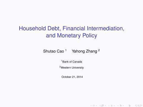
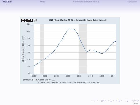
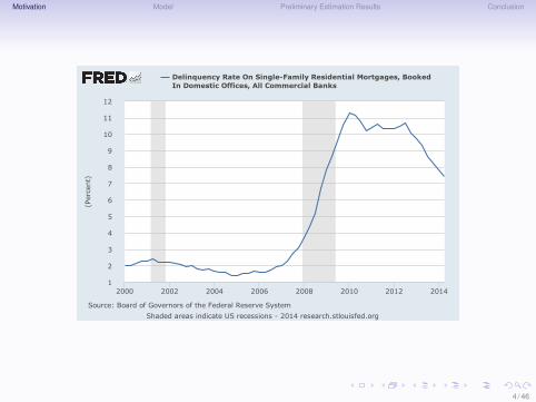
• The US experience suggests that the collapse of house pricecan be the leading factor for the recent great recession

• shape decline in house price• delinquency rate rises• both households’ and banks’ balance sheet deteriorate• rise in mortgage risk premium further worsens the problem

• This calls for a model that take into account both banks’ andhouseholds’ balance sheets

• Existing works on household debt in DSGE literature are silenton the role of banks

• exception: Iacoviello (2014)• however, it does not has a micro-foundation for why banks face the

limitation of raising deposits

2 / 46


80

100

120

140

160

180

200

220

2000 2002 2004 2006 2008 2010 2012 2014

ShadedareasindicateUSrecessions-2014research.stlouisfed.org

Source:S&PDowJonesIndicesLLC

S&P/Case-Shiller20-CityCompositeHomePriceIndex©(Index

January

2000=

100)

3 / 46


1

2

3

4

5

6

7

8

9

10

11

12

2000 2002 2004 2006 2008 2010 2012 2014

ShadedareasindicateUSrecessions-2014research.stlouisfed.org

Source:BoardofGovernorsoftheFederalReserveSystem

DelinquencyRateOnSingle-FamilyResidentialMortgages,BookedInDomesticOffices,AllCommercialBanks

(Percent)

4 / 46


5 / 46


Our Contribution

• This paper introduces a micro-founded banking sector to a DSGEmodel with agents with heterogenous desires to save and borrow

• Key features:• Two types of agents:

• patient agents: depositors• impatient agents: borrowers• enforcement problem between bankers and borrowers: collateral

constraint

• Bankers channel funds between borrowers and depositors• Gerter and Karadi (2010), agency problem between bankers and

depositors• bankers have incentive to divert funds• as long as the constraint binds, bankers demand excess return

(risk premium)

6 / 46


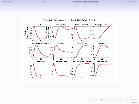
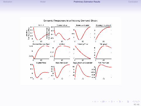
Key Mechanism – an Example

• An unexpected risk in housing demand leads to a rise in houseprice

• Household debt rises while collateral constraint for householdborrowers tightens

• Rise in house price increases bankers’ asset values• Net worth of the bankers rise• Bankers’ incentive constraint becomes less tight, leading a

decline in risk premium• The other way around for the financial crisis case

7 / 46


8 / 46


Closely Related Papers

• Financial intermediaries in business cycle: Gertler and Kiyotaki(2013), Gertler and Karadi (2011), Iacoviello (2014)

• Household debt and business cycle: Iacoviello (2005), Iacovielloand Neri (2010), and Justiniano, Primiceri and Tambalotti (2013)

9 / 46


The Model

10 / 46


Set Up of the Model

• Households: patient and impatient• patient: depositors• impatient: borrowers (subject to a collateral constraint)

• Bankers: provide funds to firms and impatient households, issuedeposits to patient households

• incentive of diverting funds• demand excess return

• Producers• competitive house producers• competitive capital producers: provide capital to wholesale goods• wholesale goods producers: use labour and capital, borrow from

bankers for capital acquisition• retailers

• Government and monetary authority• traditional Taylor rule• credit policy

11 / 46


Two types of households

• Patient households are depositors to the financial intermediariesβp

• Impatient households are borrowers from the financialintermediaries βip

• βip < βp

12 / 46


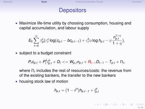
Depositors

• Maximize life-time utility by choosing consumption, housing andcapital accumulation, and labour supply

E0

∞∑t=0

βtp(εc

t log(cp,t − bcp,t−1) + εht φ log hp,t − ψ

n1+ηp,t

1 + η),

• subject to a budget constraint

Ptcp,t + Pht ihp,t + Dt <= Wp,tnp,t + Rt−1Dt−1 − Tp,t + Πt ,

where Πt includes the rest of resources/costs: the revenue fromof the existing bankers, the transfer to the new bankers

• housing stock law of motion

hp,t = (1− δh)hp,t−1 + ihp,t

13 / 46


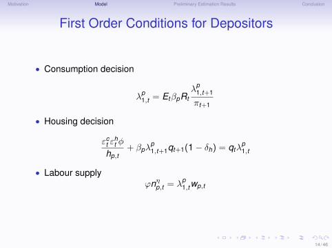
First Order Conditions for Depositors

• Consumption decision

λp1,t = EtβpRt

λp1,t+1

πt+1

• Housing decision

εct ε

ht φ

hp,t+ βpλ

p1,t+1qt+1(1− δh) = qtλ

p1,t

• Labour supplyϕnηp,t = λp

1,twp,t

14 / 46


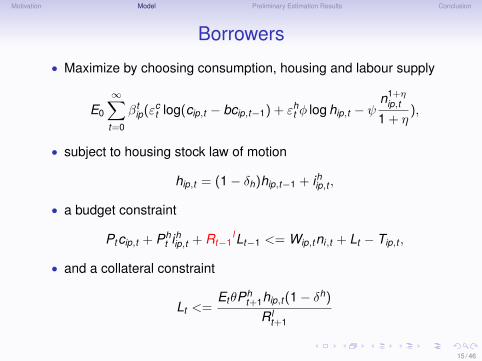
Borrowers

• Maximize by choosing consumption, housing and labour supply

E0

∞∑t=0

βtip(εc

t log(cip,t − bcip,t−1) + εht φ log hip,t − ψ

n1+ηip,t

1 + η),

• subject to housing stock law of motion

hip,t = (1− δh)hip,t−1 + ihip,t ,

• a budget constraint

Ptcip,t + Pht ihip,t + Rt−1

lLt−1 <= Wip,tni,t + Lt − Tip,t ,

• and a collateral constraint

Lt <=EtθPh

t+1hip,t (1− δh)

R lt+1

15 / 46


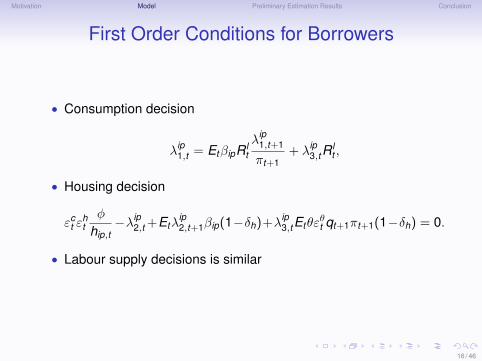
First Order Conditions for Borrowers

• Consumption decision

λip1,t = EtβipR l

t

λip1,t+1

πt+1+ λip

3,tRlt ,

• Housing decision

εct ε

htφ

hip,t−λip

2,t +Etλip2,t+1βip(1−δh)+λip

3,tEtθεθt qt+1πt+1(1−δh) = 0.

• Labour supply decisions is similar

16 / 46


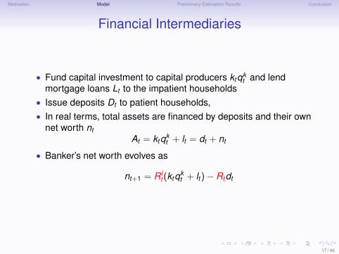
Financial Intermediaries

• Fund capital investment to capital producers ktqkt and lend

mortgage loans Lt to the impatient households• Issue deposits Dt to patient households,• In real terms, total assets are financed by deposits and their own

net worth ntAt = ktqk

t + lt = dt + nt

• Banker’s net worth evolves as

nt+1 = R lt (ktqk

t + lt )− Rtdt

17 / 46


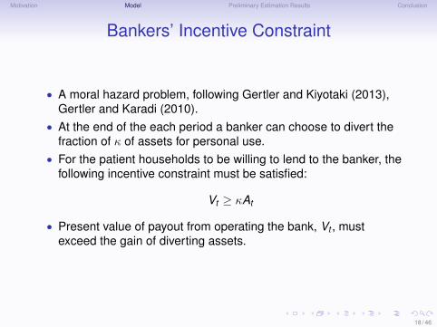
Bankers’ Incentive Constraint

• A moral hazard problem, following Gertler and Kiyotaki (2013),Gertler and Karadi (2010).

• At the end of the each period a banker can choose to divert thefraction of κ of assets for personal use.

• For the patient households to be willing to lend to the banker, thefollowing incentive constraint must be satisfied:

Vt ≥ κAt

• Present value of payout from operating the bank, Vt , mustexceed the gain of diverting assets.

18 / 46


Bankers’ Value Function

• In each period, probability σ of surviving, and a probability of1− σ of exiting

• Bankers are risk neutral and only consume (their net worth)when they exit

• Vt can be expressed recursively as

Vt = Et [β(1− σ)nt+1 + βσVt+1]

19 / 46


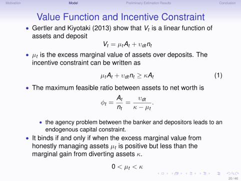
Value Function and Incentive Constraint• Gertler and Kiyotaki (2013) show that Vt is a linear function of

assets and depositVt = µtAt + υdtnt

• µt is the excess marginal value of assets over deposits. Theincentive constraint can be written as

µtAt + υdtnt ≥ κAt (1)

• The maximum feasible ratio between assets to net worth is

φt =At

nt=

υdt

κ− µt.

• the agency problem between the banker and depositors leads to anendogenous capital constraint.

• It binds if and only if when the excess marginal value fromhonestly managing assets µt is positive but less than themarginal gain from diverting assets κ.

0 < µt < κ

20 / 46


Risk Premium

• µt and υdt can be further expressed as

µt = βEt [(R lt+1 − Rt+1)Ωt+1],

υdt = βEt [Rt+1Ωt+1],

withΩt+1 = 1− σ + σ(υdt+1 + φt+1µt+1),

• Ωt+1 can be thought of as a weighted average of marginal valuesof net worth for the exiting bankers (1− σ) and surviving bankers(σ).

21 / 46


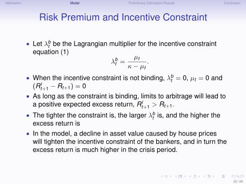
Risk Premium and Incentive Constraint

• Let λbt be the Lagrangian multiplier for the incentive constraint

equation (1)λb

t =µt

κ− µt.

• When the incentive constraint is not binding, λbt = 0, µt = 0 and

(R lt+1 − Rt+1) = 0

• As long as the constraint is binding, limits to arbitrage will lead toa positive expected excess return, R l

t+1 > Rt+1.

• The tighter the constraint is, the larger λbt is, and the higher the

excess return is• In the model, a decline in asset value caused by house prices

will tighten the incentive constraint of the bankers, and in turn theexcess return is much higher in the crisis period.

22 / 46


Aggregate Net Worth

• At aggregate level, banker’s net worth evolves as

n = nnt + ne

t

withne

t = σ[(R lt − Rt )φt + Rt ]ne

t−1

andnn

t = ωAt−1

23 / 46


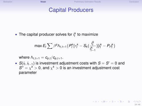
Capital Producers

• The capital producer solves for ikt to maximize

max Et

∑βpΛt,t+1Pk

t [τ kt − Sk (

iktikt−1

)]ikt − Pt ikt

where Λt,t+1 = cp,t/cp,t+1.• S(it , it−1) is investment adjustment costs with S = S′ = 0 and

S′′ = χk > 0, and χk > 0 is an investment adjustment costparameter

24 / 46


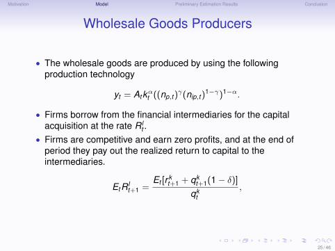
Wholesale Goods Producers

• The wholesale goods are produced by using the followingproduction technology

yt = Atkαt ((np,t )γ(nip,t )

1−γ)1−α.

• Firms borrow from the financial intermediaries for the capitalacquisition at the rate R l

t .• Firms are competitive and earn zero profits, and at the end of

period they pay out the realized return to capital to theintermediaries.

EtR lt+1 =

Et [r kt+1 + qk

t+1(1− δ)]

qkt

,

25 / 46


Wholesale Goods Producers

• Each period, firms maximize the profit by choosing kt ,np,t andnip,t

max pwt Yt − r k

t kt − wp,tnp,t − wip,tnip,t

and the first-order conditions are

pwt α

Yt

kt= r k

t ,

pwt αγ

Yt

np,t= wp,t ,

andpw

t α(1− γ)Yt

np,t= wip,t

where pwt is the price for the wholesale goods.

26 / 46


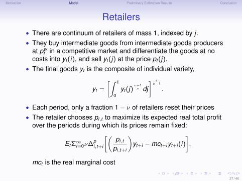
Retailers• There are continuum of retailers of mass 1, indexed by j .• They buy intermediate goods from intermediate goods producers

at pwt in a competitive market and differentiate the goods at no

costs into yt (i), and sell yt (j) at the price pt (j).• The final goods yt is the composite of individual variety,

yt =

[∫ 1

0yt (j)

ε−1ε dj

] εε−1

.

• Each period, only a fraction 1− ν of retailers reset their prices• The retailer chooses pi,t to maximize its expected real total profit

over the periods during which its prices remain fixed:

Et Σ∞i=0ν∆p

i,t+i

[(pi,t

pi,t+i

)yt+i −mct+iyt+i (i)

],

mct is the real marginal cost

27 / 46


House Producers

• The production of new house

hnt = (τh

t − Sh(iht

iht−1))iht ,

• The house producer solves for iht to maximize

max Et

∑βpΛt,t+1[Ph

t hnt − Pt iht ]

where Λt,t+1 = cp,t/cp,t+1.

28 / 46


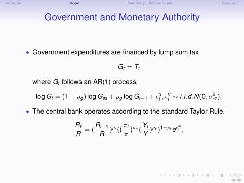
Government and Monetary Authority

• Government expenditures are financed by lump sum tax

Gt = Tt

where Gt follows an AR(1) process,

log Gt = (1− ρg) log Gss + ρg log Gt−1 + εgt , ε

gt ∼ i .i .d .N(0, σ2

εg ).

• The central bank operates according to the standard Taylor Rule.

Rt

R= (

Rt−1

R)ρr ((

πt

π)ρπ (

Yt

Y)ρy )1−ρr eε

mt ,

29 / 46


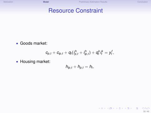
Resource Constraint

• Goods market:

cp,t + cip,t + qt (ihp,t + ihip,t ) + qkt ikt = y f

t ,

• Housing market:hip,t + hp,t = ht ,

30 / 46


Data and Estimation

31 / 46


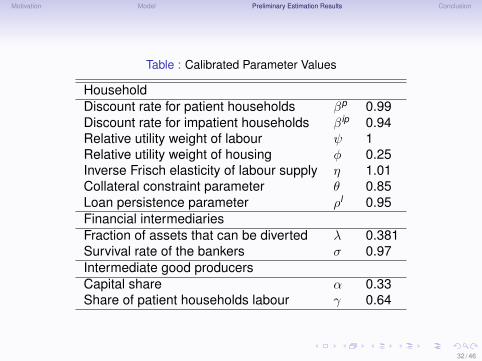
Table : Calibrated Parameter Values

HouseholdDiscount rate for patient households βp 0.99Discount rate for impatient households β ip 0.94Relative utility weight of labour ψ 1Relative utility weight of housing φ 0.25Inverse Frisch elasticity of labour supply η 1.01Collateral constraint parameter θ 0.85Loan persistence parameter ρl 0.95Financial intermediariesFraction of assets that can be diverted λ 0.381Survival rate of the bankers σ 0.97Intermediate good producersCapital share α 0.33Share of patient households labour γ 0.64

32 / 46


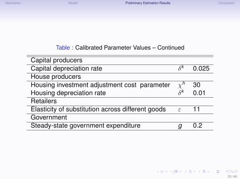
Table : Calibrated Parameter Values – Continued

Capital producersCapital depreciation rate δk 0.025House producersHousing investment adjustment cost parameter χh 30Housing depreciation rate δk 0.01RetailersElasticity of substitution across different goods ε 11GovernmentSteady-state government expenditure g 0.2

33 / 46


Data Used

• output, consumption, business investment, government spending• nominal interest rate, inflation• mortgage risk premium, mortgage loan

34 / 46


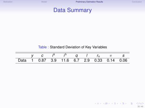
Data Summary

Table : Standard Deviation of Key Variables

y c ik ih q l rn π sData 1 0.87 3.9 11.6 6.7 2.9 0.33 0.14 0.06

35 / 46


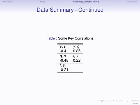
Data Summary –Continued

Table : Some Key Correlations

y , s y ,q-0.4 0.85q, s q, l-0.48 0.22l , s-0.21

36 / 46


Shocks Estimated

• technology, monetary policy, preference, investment specific andgovernment spending shocks

• housing preference shock, LTV shock• bank net worth shock

37 / 46


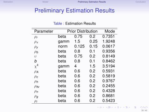
Preliminary Estimation Results

Table : Estimation Results

Parameter Prior Distribution Modeρr beta 0.75 0.2 0.7351ρπ gamm 1.5 0.25 1.9248ρy norm 0.125 0.15 0.0617ρb beta 0.8 0.1 0.9356υ beta 0.75 0.2 0.8149b beta 0.8 0.1 0.8462χk gamm 4 1.5 3.5194ρA beta 0.6 0.2 0.5931ρc beta 0.6 0.2 0.5819ρh beta 0.6 0.2 0.9767ρltv beta 0.6 0.2 0.2455ρn beta 0.6 0.2 0.4328ρg beta 0.6 0.2 0.8681ρi beta 0.6 0.2 0.5423

38 / 46


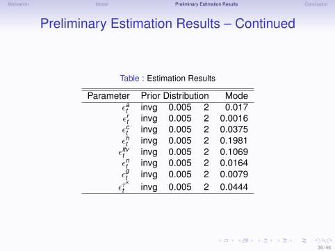
Preliminary Estimation Results – Continued

Table : Estimation Results

Parameter Prior Distribution Modeεat invg 0.005 2 0.017εrt invg 0.005 2 0.0016εct invg 0.005 2 0.0375εht invg 0.005 2 0.1981εltvt invg 0.005 2 0.1069εnt invg 0.005 2 0.0164ε

gt invg 0.005 2 0.0079

ετk

t invg 0.005 2 0.0444

39 / 46


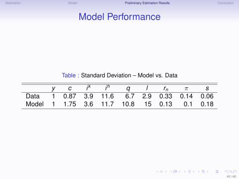
Model Performance

Table : Standard Deviation – Model vs. Data

y c ik ih q l rn π sData 1 0.87 3.9 11.6 6.7 2.9 0.33 0.14 0.06Model 1 1.75 3.6 11.7 10.8 15 0.13 0.1 0.18

40 / 46


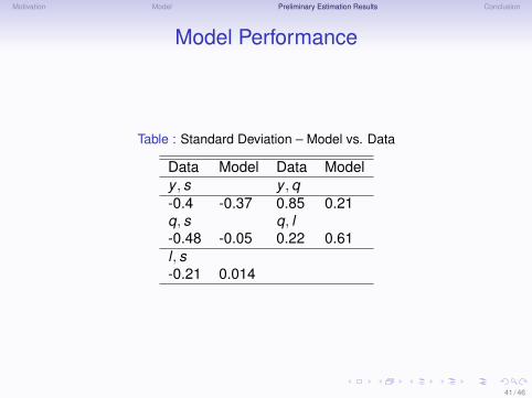
Model Performance

Table : Standard Deviation – Model vs. Data

Data Model Data Modely , s y ,q-0.4 -0.37 0.85 0.21q, s q, l-0.48 -0.05 0.22 0.61l , s-0.21 0.014

41 / 46


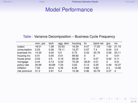
Model Performance

Table : Variance Decomposition – Business Cycle Frequency

mon. pol. tech agg. dem housing ltv bank net gov invoutput 18.01 1.28 23.93 16.29 0.47 17.25 1.62 21.15consumption 0.23 0.36 79.11 12.27 0.07 7.4 0.04 0.5business inv. 14.35 0.04 0.5 0.75 0.43 30.76 0.06 53.11housing inv. 0.01 0.05 0.01 99.92 0 0 0 0.01house price 0.03 0.5 0.18 99.09 0 0.07 0.02 0.11mortgage 0.44 0.13 0.22 70.39 28.81 0.01 0 0.01policy rate 30.99 40.89 7.24 3.63 0.13 0.25 0.49 16.37inflation 7.93 64.6 4.35 8.26 0.68 0.82 0.3 13.06risk premium 31.3 3.91 5.4 10.38 0.96 43.78 0.27 4

42 / 46


43 / 46


44 / 46


45 / 46


Conclusions

• We introduces a micro-founded banking sector to a DSGE modelwith agents with heterogenous desires to save and borrow

• In the model collateral constraint and risk premium co-exist• Preliminary results show that

• model generates counter cyclical risk premium• bank net worth shocks are important in explaining output,

mortgage risk premium and business investment• Loan-to-Value ratio shocks are important in explaining mortgage

46 / 46

household debt, financial intermediation, and monetary...

Documents