escher’s circle limit iii - cs.brown.edu · nonlinear svms the kernel trick: instead of...
TRANSCRIPT


Escher’s Circle Limit III

Escher’s Circle Limit III
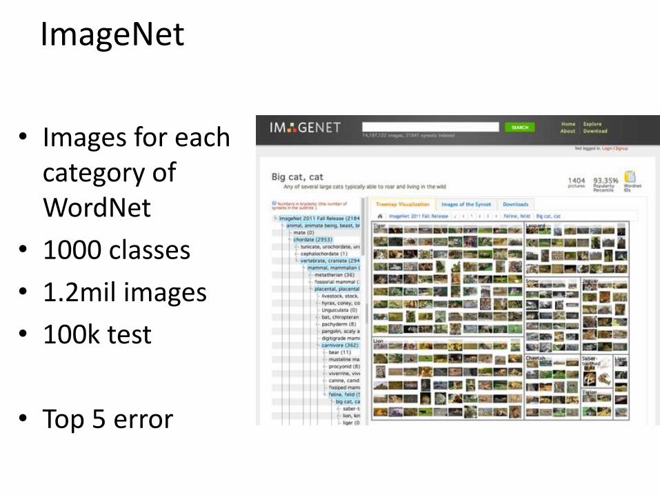
ImageNet
• Images for each category of WordNet
• 1000 classes
• 1.2mil images
• 100k test
• Top 5 error

Dataset split
Training
Images
Testing
Images
Validation
Images
- Secret labels- Measure error
- Train classifier - Measure error- Tune model hyperparameters
Random train/validate splits = cross validation
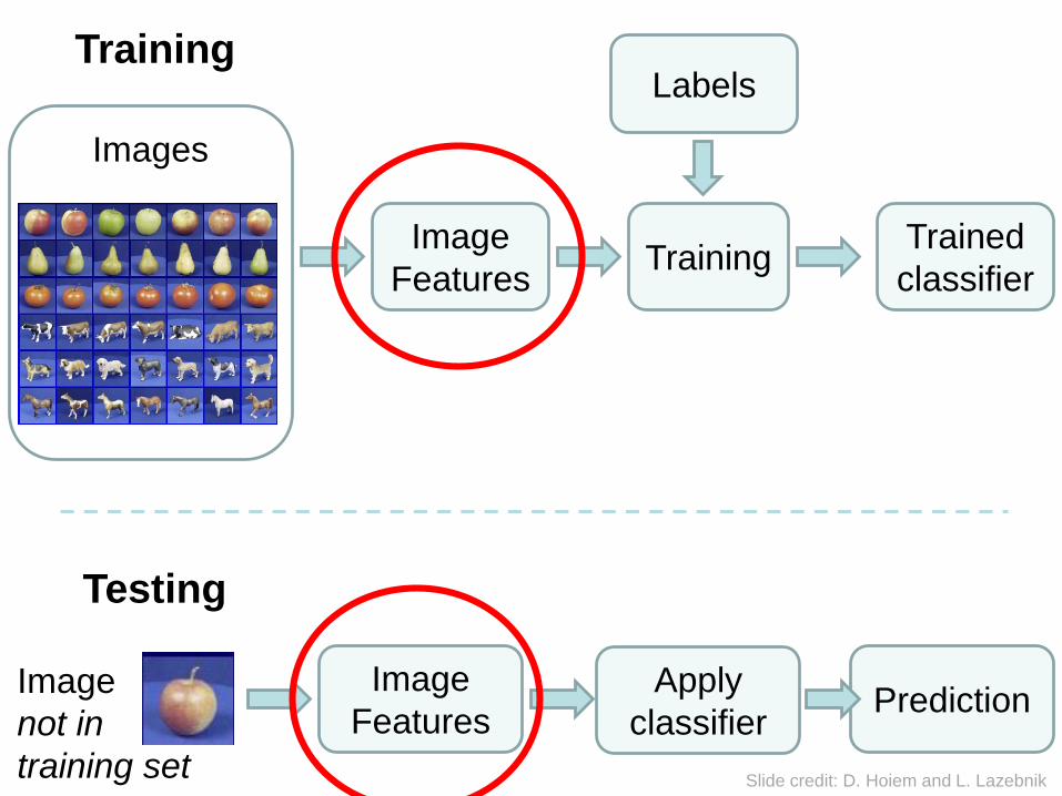
Prediction
Labels
Images
Training
Training
Image
Features
Image
Features
Testing
Image
not in
training set
Trained
classifier
Apply
classifier
Slide credit: D. Hoiem and L. Lazebnik
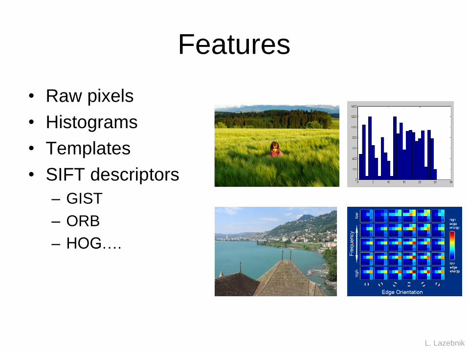
Features
• Raw pixels
• Histograms
• Templates
• SIFT descriptors
– GIST
– ORB
– HOG….
L. Lazebnik

Prediction
Labels
Images
Training
Training
Image
Features
Image
Features
Testing
Image
not in
training set
Trained
classifier
Apply
classifier
Slide credit: D. Hoiem and L. Lazebnik

Think-Pair-Share
What are all the possible supervision (‘label’) types to consider?
Recognition task and supervision
L. Lazebnik

• Images in the training set must be annotated with the
“correct answer” that the model is expected to produce
Contains a motorbike
Recognition task and supervision
L. Lazebnik

Unsupervised “Weakly” supervised Fully supervised
Fuzzy; definition depends on task
Lazebnik
Spectrum of supervision
Less More
E.G., MS CocoE.G., ImageNet
‘Semi-supervised’: small partial labeling

Good training
example?

Good labels?
http://mscoco.org/explore/?id=134918

Google guesses from the 1st caption

Prediction
Labels
Images
Training
Training
Image
Features
Image
Features
Testing
Image
not in
training set
Trained
classifier
Apply
classifier
Slide credit: D. Hoiem and L. Lazebnik

The machine learning framework
• Apply a prediction function to a feature representation of
the image to get the desired output:
f( ) = “apple”
f( ) = “tomato”
f( ) = “cow”Slide credit: L. Lazebnik
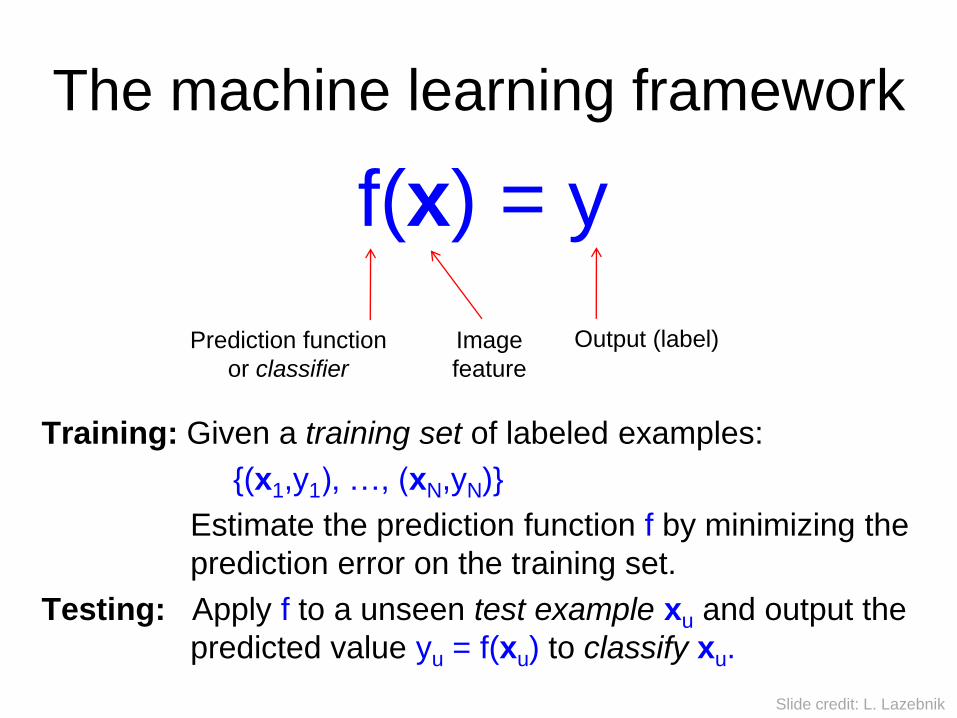
The machine learning framework
f(x) = y
Training: Given a training set of labeled examples:
{(x1,y1), …, (xN,yN)}
Estimate the prediction function f by minimizing the
prediction error on the training set.
Testing: Apply f to a unseen test example xu and output the
predicted value yu = f(xu) to classify xu.
Output (label)Prediction function
or classifier
Image
feature
Slide credit: L. Lazebnik

ClassificationAssign x to one of two (or more) classes.
A decision rule divides input space into decision
regions separated by decision boundaries – literally
boundaries in the space of the features.
L. Lazebnik

Classifiers: Nearest neighbor
f(x) = label of the training example nearest to x
• All we need is a distance function for our inputs
• No training required!
Test
exampleTraining
examples
from class 1
Training
examples
from class 2
Slide credit: L. Lazebnik
Quickie Think-Pair-Share: What does the decision boundary look like?

ClassificationAssign x to one of two (or more) classes.
A decision rule divides input space into decision
regions separated by decision boundaries – literally
boundaries in the space of the features.
L. Lazebnik

Decision boundary for Nearest Neighbor Classifier
Divides input space into decision regions separated by decision boundaries – Voronoi.
Voronoi partitioning of feature space for two-category 2D and 3D data
from Duda et al. Source: D. Lowe

k-nearest neighbor
x x
xx
x
x
x
xo
oo
o
o
o
o
x2
x1
+
+
x x
xx
x
x
x
xo
oo
o
o
o
o
x2
x1
+
+
1-nearest
x x
xx
x
x
x
xo
oo
o
o
o
o
x2
x1
+
+
3-nearest
x x
xx
x
x
x
xo
oo
o
o
o
o
x2
x1
+
+
5-nearest

Classifiers: Linear
Find a linear function to separate the classes
Slide credit: L. Lazebnik
Training
examples
from class 1
Training
examples
from class 2
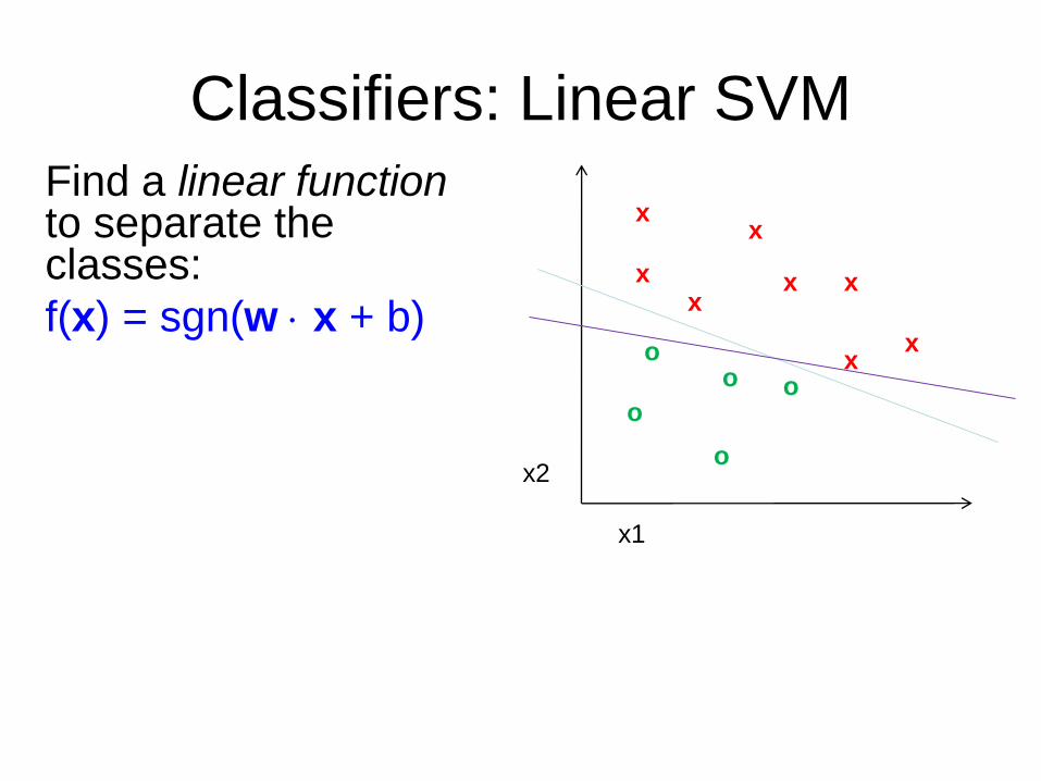
Classifiers: Linear SVM
x x
xx
x
x
x
x
oo
o
o
o
x2
x1
Find a linear function to separate the classes:
f(x) = sgn(w x + b)
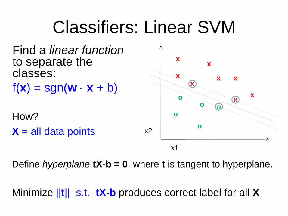
Classifiers: Linear SVM
x x
xx
x
x
x
x
oo
o
o
o
x2
x1
Find a linear function to separate the classes:
f(x) = sgn(w x + b)
How?
X = all data points
Define hyperplane tX-b = 0, where t is tangent to hyperplane.
Minimize ||t|| s.t. tX-b produces correct label for all X

Classifiers: Linear SVM
x x
xx
x
x
x
x
o
oo
o
o
o
x2
x1
Find a linear function to separate the classes:
f(x) = sgn(w x + b)
What if my data are not linearly separable?
Introduce flexible ‘hinge’ loss (or ‘soft-margin’)

• Datasets that are linearly separable work out great:
• But what if the dataset is just too hard?
• We can map it to a higher-dimensional space:
0 x
0 x
0 x
x2
Nonlinear SVMs
Andrew Moore

Φ: x→ φ(x)
Nonlinear SVMs
Map the original input space to some higher-
dimensional feature space where the training set
is separable:
Slide credit: Andrew Moore

Nonlinear SVMs
The kernel trick: instead of explicitly computing the lifting
transformation φ(x), define a kernel function K such that:
K(xi,xj) = φ(xi ) · φ(xj)
This gives a non-linear decision boundary in the original
feature space:
bKybyi
iii
i
iii +=+ ),()()( xxxx
C. Burges, A Tutorial on Support Vector Machines for Pattern Recognition
Data Mining and Knowledge Discovery, 1998
Common kernel function: Radial basis function kernel
But…we only transformed the distance function K!
[Additional info]

Nonlinear kernel: Example
Consider the mapping ),()( 2xxx =
22
2222
),(
),(),()()(
yxxyyxK
yxxyyyxxyx
+=
+==
x2
[Additional info]
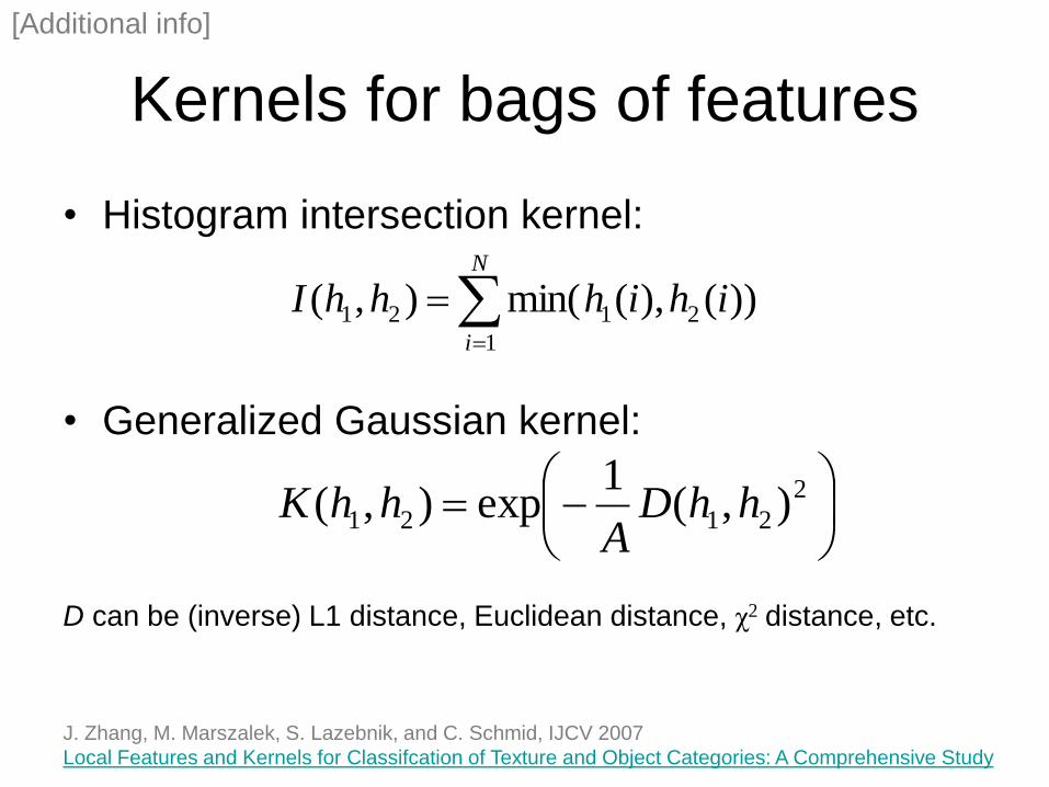
Kernels for bags of features
• Histogram intersection kernel:
• Generalized Gaussian kernel:
D can be (inverse) L1 distance, Euclidean distance, χ2 distance, etc.
=
=N
i
ihihhhI1
2121 ))(),(min(),(
−= 2
2121 ),(1
exp),( hhDA
hhK
J. Zhang, M. Marszalek, S. Lazebnik, and C. Schmid, IJCV 2007
Local Features and Kernels for Classifcation of Texture and Object Categories: A Comprehensive Study
[Additional info]

What about multi-class SVMs?
Unfortunately, there is no “definitive” multi-class SVM.
In practice, we combine multiple two-class SVMs
One vs. others
– Training: learn an SVM for each class vs. the others
– Testing: apply each SVM to test example and assign to it the
class of the SVM that returns the highest decision value
One vs. one
– Training: learn an SVM for each pair of classes
– Testing: each learned SVM “votes” for a class to assign to the
test example
Slide credit: L. Lazebnik

SVMs: Pros and cons
• Pros
– Many publicly available SVM packages:
http://www.kernel-machines.org/software
– Kernel-based framework is very powerful, flexible
– SVMs work very well in practice, even with very small
training sample sizes
• Cons
– No “direct” multi-class SVM, must combine two-class SVMs
– Computation, memory
• During training time, must compute matrix of kernel
values for every pair of examples
• Learning can take a very long time for large-scale
problems

Prediction
Training
LabelsTraining
Images
Training
Training
Image
Features
Image
Features
Testing
Test Image
Learned
classifier
Apply
classifier
Slide credit: D. Hoiem and L. Lazebnik

Features and distance measures
define visual similarity.
Training labels
dictate that examples are the same or different.
Classifiers
learn weights (or parameters) of features and
distance measures…
so that visual similarity predicts label similarity.

Generalization
How well does a learned model generalize from the
data it was trained on to a new test set?
Training set (labels known) Test set (labels
unknown)
Slide credit: L. Lazebnik
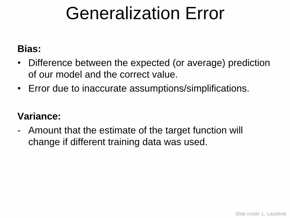
Generalization Error
Bias:
• Difference between the expected (or average) prediction
of our model and the correct value.
• Error due to inaccurate assumptions/simplifications.
Variance:
- Amount that the estimate of the target function will
change if different training data was used.
Slide credit: L. Lazebnik

Bias/variance trade-off
[Scott Fortmann-Roe]
Bias = accuracy
Variance = precision
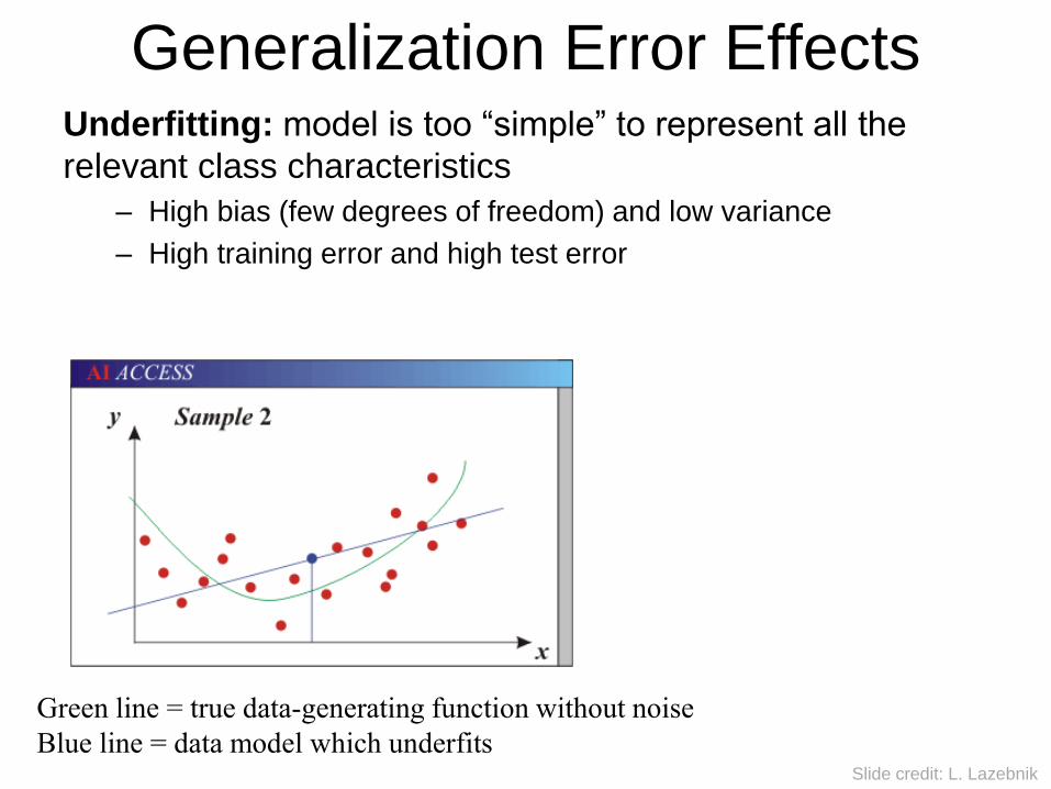
Generalization Error EffectsUnderfitting: model is too “simple” to represent all the
relevant class characteristics
– High bias (few degrees of freedom) and low variance
– High training error and high test error
Slide credit: L. Lazebnik
Green line = true data-generating function without noise
Blue line = data model which underfits

Generalization Error EffectsOverfitting: model is too “complex” and fits irrelevant
characteristics (noise) in the data
– Low bias (many degrees of freedom) and high variance
– Low training error and high test error
Slide credit: L. Lazebnik
Green line = true data-generating function without noise
Blue line = data model which overfits

Bias-Variance Trade-off
Models with too few parameters are inaccurate because of a large bias.
• Not enough flexibility!
• Too many assumptions
Models with too many parameters are inaccurate because of a large variance.
• Too much sensitivity to the sample.
• Slightly different data -> very different function.
Slide credit: D. Hoiem
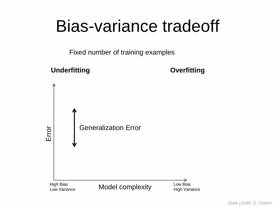
Bias-variance tradeoff
Training error
Test error
Underfitting Overfitting
Model complexityLow Bias
High Variance
High Bias
Low Variance
Err
or
Slide credit: D. Hoiem
Generalization Error
Fixed number of training examples

Bias-variance tradeoff
Many training examples
Few training examples
Low Bias
High Variance
High Bias
Low Variance
Test E
rror
Slide credit: D. Hoiem
Overfitting
Underfitting
Model complexity

Effect of Training Size
Testing
Training
Number of Training Examples
Err
or
Fixed complexity prediction model
Slide credit: D. Hoiem

[evolvingai.org]
“Learn the data boundary” “Represent the data and then define boundary”
Given: Observations XTargets Y
Learn conditional distribution:𝑃(𝑌|𝑋 = 𝑥)
Given: Observations XTargets Y
Learn joint distribution:𝑃(𝑋, 𝑌)

Slides: James Hays, Isabelle Guyon, Erik Sudderth,
Mark Johnson, Derek Hoiem
Photo: CMU Machine Learning Department Protests G20

Many classifiers to choose from…
• K-nearest neighbor
• SVM
• Naïve Bayes
• Bayesian network
• Logistic regression
• Randomized Forests
• Boosted Decision Trees
• Restricted Boltzmann Machines
• Neural networks
• Deep Convolutional Network
• …
Which is
the best?
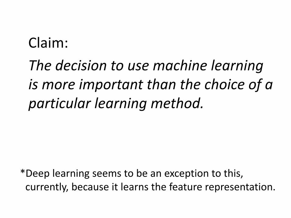
Claim:
The decision to use machine learning is more important than the choice of a particular learning method.
*Deep learning seems to be an exception to this, currently, because it learns the feature representation.

*Again, deep learning may be an exception here for the same reason, but deep learning _needs_ a lot of labeled data in the first place.
“The Unreasonable Effectiveness of Data” - Norvig
Claim:
It is more important to have more or better labeled data than to use a different supervised learning technique.

What to remember about classifiers
• No free lunch: machine learning algorithms are tools, not dogmas
• Try simple classifiers first
• Better to have smart features and simple classifiers than simple features and smart classifiers
• Use increasingly powerful classifiers with more training data (bias-variance tradeoff)
Slide credit: D. Hoiem