kernel methods and svms - umass amherstdomke/courses/sml2011/07kernels.pdf · kernel methods and...
TRANSCRIPT

Statistical Machine Learning Notes 7
Kernel Methods and SVMs
Instructor: Justin Domke
Contents
1 Introduction 2
2 Kernel Ridge Regression 2
3 The Kernel Trick 5
4 Support Vector Machines 7
5 Examples 10
6 Kernel Theory 16
6.1 Kernel algebra . . . . . . . . . . . . . . . . . . . . . . . . . . . . . . . . . . . 16
6.2 Understanding Polynomial Kernels via Kernel Algebra . . . . . . . . . . . . 18
6.3 Mercer’s Theorem . . . . . . . . . . . . . . . . . . . . . . . . . . . . . . . . . 19
7 Our Story so Far 21
8 Discussion 22
8.1 SVMs as Template Methods . . . . . . . . . . . . . . . . . . . . . . . . . . . 22
8.2 Theoretical Issues . . . . . . . . . . . . . . . . . . . . . . . . . . . . . . . . . 23
1

Kernel Methods and SVMs 2
1 Introduction
Support Vector Machines (SVMs) are a very succesful and popular set of techniques forclassification. Historically, SVMs emerged after the neural network boom of the 80s andearly 90s. People were surprised to see that SVMs with little to no “tweaking” could competewith neural networks involving a great deal of manual engineering.
It remains true today that SVMs are among the best “off-the-shelf” classification methods.If you want to get good results with a minimum of messing around, SVMs are a very goodchoice.
Unlike the other classification methods we discuss, it is not convenient to begin with a concisedefinition of SVMs, or even to say what exactly a “support vector” is. There is a set of ideasthat must be understood first. Most of these you have already seen in the notes on linearmethods, basis expansions, and template methods. The biggest remaining concept is knownas the kernel trick. In fact, this idea is so fundamental many people have advocated thatSVMs be renamed “Kernel Machines”.
It is worth mentioning that the standard presentation of SVMs is based on the concept of“margin”. For lack of time, this perspective on SVMs will not be presented here. If you willbe working seriously with SVMs, you should familiarize yourself with the margin perspectiveto enjoy a full understanding.
(Warning: These notes are probably the most technically challenging in this course, par-ticularly if you don’t have a strong background in linear algebra, Lagrange multipliers, andoptimization. Kernel methods simply use more mathematical machinery than most of theother techniques we cover, so you should be prepared to put in some extra effort. Enjoy!)
2 Kernel Ridge Regression
We begin by not talking about SVMs, or even about classification. Instead, we revisit ridgeregression, with a slight change of notation. Let the set of inputs be {(xi, yi)}, where iindexes the samples. The problem is to minimize
∑
i
(
xi · w − yi
)2+ λw ·w
If we take the derivative with respect to w and set it to zero, we get
Kernel Methods and SVMs 3
0 =∑
i
2xi(xTi w − yi) + 2λw
w =(
∑
i
xixTi + λI
)−1∑
i
xiyi.
Now, let’s consider a different derivation, making use of some Lagrange duality. If we in-troduce a new variable zi, and constrain it to be the difference between w · xi and yi, wehave
minw,z
1
2z · z +
1
2λw · w (2.1)
s.t. zi = xi · w − yi.
Using αi to denote the Lagrange multipliers, this has the Lagrangian
L =1
2z · z +
1
2λw · w +
∑
i
αi(xi ·w − yi − zi).
Recall our foray into Lagrange duality. We can solve the original problem by doing
maxα
minw,z
L(w, z, α).
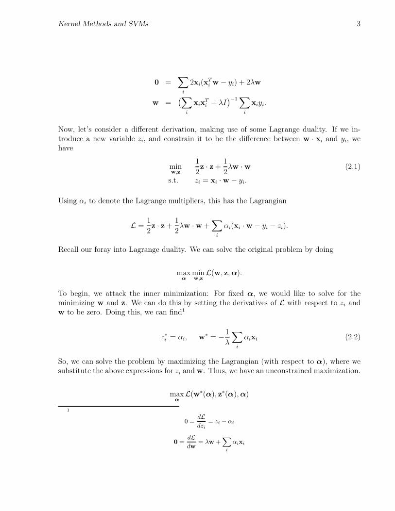
To begin, we attack the inner minimization: For fixed α, we would like to solve for theminimizing w and z. We can do this by setting the derivatives of L with respect to zi andw to be zero. Doing this, we can find1
z∗i = αi, w∗ = −1
λ
∑
i
αixi (2.2)
So, we can solve the problem by maximizing the Lagrangian (with respect to α), where wesubstitute the above expressions for zi and w. Thus, we have an unconstrained maximization.
maxα
L(w∗(α), z∗(α), α)
1
0 =dLdzi
= zi − αi
0 =dLdw
= λw +∑
i
αixi

Kernel Methods and SVMs 4
Before diving into the details of that, we can already notice something very interestinghappening here: w is given by a sum of the input vectors xi, weighted by −αi/λ. If we wereso inclined, we could avoid explicitly computing w, and predict a new point x directly fromthe data as
f(x) = x · w = −1
λ
∑
i
αix · xi.
Now, let k(xi,xj) = xi · xj be the “kernel function”. For now, just think of this as a changeof notation. Using this, we can again write the ridge regression predictions as
f(x) = −1
λ
∑
i
αik(x,xi).
Thus, all we really need is the inner product of x with each of the training elements xi. Wewill return to why this might be useful later. First, let’s return to doing the maximizationover the Lagrange multipliers α, to see if anything similar happens there. The math belowlooks really complicated. However, all the we are doing is substituting the expressions forz∗i and w∗ from Eq. 2.2, then doing a lot of manipulation.
maxα
minw,z
L = maxα
1
2
∑
i
α2
i +1
2λ(
−1
λ
∑
i
αixi
)
·(
−1
λ
∑
j
αjxj
)
+∑
i
αi(xi · −1
λ
∑
j
αjxj − yi − αi)
= maxα
1
2
∑
i
α2
i +1
2λ
∑
i
∑
j
αiαjxi · xj −1
λ
∑
i
∑
j
αiαjxi · xj −∑
i
αi(yi + αi)
= maxα
−1
2
∑
i
α2
i −1
2λ
∑
i
∑
j
αiαjxi · xj −∑
i
αiyi
= maxα
−1
2
∑
i
α2
i −1
2λ
∑
i
∑
j
αiαjk(xi,xj) −∑
i
αiyi.
Again, we only need inner products. If we define the matrix K by
Kij = k(xi,xj),
then we can rewrite this in a punchier vector notation as
Kernel Methods and SVMs 5
maxα
minw,z
L = maxα
−1
2α · α − 1
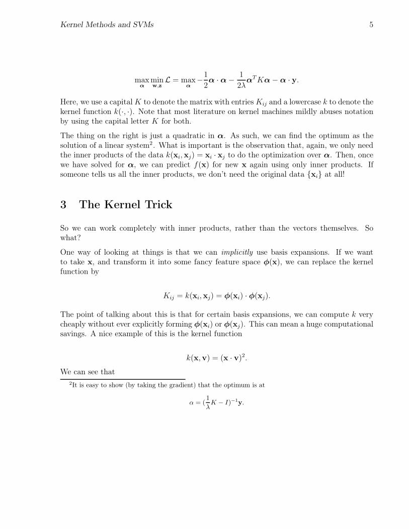
2λαT Kα − α · y.
Here, we use a capital K to denote the matrix with entries Kij and a lowercase k to denote thekernel function k(·, ·). Note that most literature on kernel machines mildly abuses notationby using the capital letter K for both.
The thing on the right is just a quadratic in α. As such, we can find the optimum as thesolution of a linear system2. What is important is the observation that, again, we only needthe inner products of the data k(xi,xj) = xi · xj to do the optimization over α. Then, oncewe have solved for α, we can predict f(x) for new x again using only inner products. Ifsomeone tells us all the inner products, we don’t need the original data {xi} at all!
3 The Kernel Trick
So we can work completely with inner products, rather than the vectors themselves. Sowhat?
One way of looking at things is that we can implicitly use basis expansions. If we wantto take x, and transform it into some fancy feature space φ(x), we can replace the kernelfunction by
Kij = k(xi,xj) = φ(xi) · φ(xj).
The point of talking about this is that for certain basis expansions, we can compute k verycheaply without ever explicitly forming φ(xi) or φ(xj). This can mean a huge computationalsavings. A nice example of this is the kernel function
k(x,v) = (x · v)2.
We can see that
2It is easy to show (by taking the gradient) that the optimum is at
α = (1
λK − I)−1y.
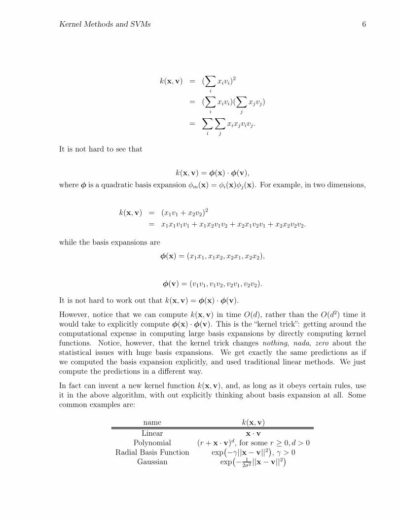
Kernel Methods and SVMs 6
k(x,v) = (∑
i
xivi)2
= (∑
i
xivi)(∑
j
xjvj)
=∑
i
∑
j
xixjvivj .
It is not hard to see that
k(x,v) = φ(x) · φ(v),
where φ is a quadratic basis expansion φm(x) = φi(x)φj(x). For example, in two dimensions,
k(x,v) = (x1v1 + x2v2)2
= x1x1v1v1 + x1x2v1v2 + x2x1v2v1 + x2x2v2v2.
while the basis expansions are
φ(x) = (x1x1, x1x2, x2x1, x2x2),
φ(v) = (v1v1, v1v2, v2v1, v2v2).
It is not hard to work out that k(x,v) = φ(x) · φ(v).
However, notice that we can compute k(x,v) in time O(d), rather than the O(d2) time itwould take to explicitly compute φ(x) · φ(v). This is the “kernel trick”: getting around thecomputational expense in computing large basis expansions by directly computing kernelfunctions. Notice, however, that the kernel trick changes nothing, nada, zero about thestatistical issues with huge basis expansions. We get exactly the same predictions as ifwe computed the basis expansion explicitly, and used traditional linear methods. We justcompute the predictions in a different way.
In fact can invent a new kernel function k(x,v), and, as long as it obeys certain rules, useit in the above algorithm, with out explicitly thinking about basis expansion at all. Somecommon examples are:
name k(x,v)
Linear x · vPolynomial (r + x · v)d, for some r ≥ 0, d > 0
Radial Basis Function exp(
−γ||x − v||2)
, γ > 0Gaussian exp
(
− 1
2σ2 ||x − v||2)

Kernel Methods and SVMs 7
We will return below to the question of what kernel functions are “legal”, meaning there issome feature space φ such that k(x,v) = φ(x) · φ(v).
Now, what exactly was it about ridge regression that let us get away with working entirelywith inner products? How much could we change the problem, and preserve this? We reallyneed two things to happen:
1. When we take dL/dw = 0, we need to be able to solve for w, and the solution needsto be a linear combination of the input vectors xi.
2. When we substitute this solution back into the Lagrangian, we need to get a solutionthat simplifies down into inner products only.
Notice that this leaves us a great deal of flexibility. For example, we could replace the least-squares criterion z · z with an alternative (convex) measure. We could also change the wayin which which measure errors from zi = w ·xi − yi, to something else, (although with somerestrictions).
4 Support Vector Machines
Now, we turn to the binary classification problem. Support Vector Machines result fromminimizing the hinge loss (1 − yiw · xi)+ with ridge regularization.
minw
∑
i
(1 − yiw · xi)+ + λ||w||2.
This is equivalent to (for c = 2/λ)
minw
c∑
i
(1 − yiw · xi)+ +1
2||w||2.
Because the hinge loss is non-differentiable, we introduce new variables zi, creating a con-strained optimization
minz,w
c∑
i
zi +1
2||w||2 (4.1)
s.t. zi ≥ (1 − yiw · xi)
zi ≥ 0.
Kernel Methods and SVMs 8
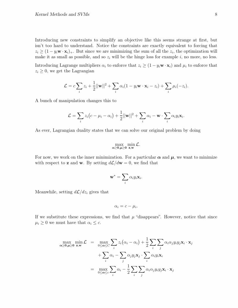
Introducing new constraints to simplify an objective like this seems strange at first, butisn’t too hard to understand. Notice the constraints are exactly equivalent to forcing thatzi ≥ (1− yiw ·xi)+. But since we are minimizing the sum of all the zi, the optimization willmake it as small as possible, and so zi will be the hinge loss for example i, no more, no less.
Introducing Lagrange multipliers αi to enforce that zi ≥ (1− yiw ·xi) and µi to enforce thatzi ≥ 0, we get the Lagrangian
L = c∑
i
zi +1
2||w||2 +
∑
i
αi(1 − yiw · xi − zi) +∑
i
µi(−zi).
A bunch of manipulation changes this to
L =∑
i
zi
(
c − µi − αi
)
+1
2||w||2 +
∑
i
αi −w ·∑
i
αiyixi.
As ever, Lagrangian duality states that we can solve our original problem by doing
maxα≥0,µ≥0
minz,w
L.
For now, we work on the inner minimization. For a particular α and µ, we want to minimizewith respect to z and w. By setting dL/dw = 0, we find that
w∗ =∑
i
αiyixi.
Meanwhile, setting dL/dzi gives that
αi = c − µi.
If we substitute these expressions, we find that µ “disappears”. However, notice that sinceµi ≥ 0 we must have that αi ≤ c.
maxα≥0,µ≥0
minz,w
L = max0≤α≤C
∑
i
zi
(
αi − αi
)
+1
2
∑
i
∑
j
αiαjyiyjxi · xj
+∑
i
αi −∑
j
αjyjxj ·∑
i
αiyixi
= max0≤α≤c
∑
i
αi −1
2
∑
i
∑
j
αiαjyiyjxi · xj

Kernel Methods and SVMs 9
This is a maximization of a quadratic objective, under linear constraints. That is, this is aquadratic program. Historically, QP solvers were first used to solve SVM problems. However,as these scale poorly to large problems, a huge amount of effort has been devoted to fastersolvers. (Often based on coordinate ascent and/or online optimization). This area is stillevolving. However, software is widely available now for solvers that are quite fast in practice.
Now, as we saw above that w =∑
i αiyixi, we can classify new points x by
f(x) =∑
i
αiyix · xi
Clearly, this can be kernelized. If we do so, we can compute the Lagrange multipliers by the
SVM optimization
max0≤α≤c
∑
i
αi −1
2
∑
i
∑
j
αiαjyiyjk(xi,xj), (4.2)
which is again a quadratic program. We can classify new points by the SVM classification
rule
f(x) =∑
i
αiyik(x,xi). (4.3)
Since we have “kernelized” both the learning optimization, and the classification rule, we areagain free to replace k with any of the variety of kernel functions we saw before.
Now, finally, we can define what a “support vector” is. Notice that Eq. 4.2 is the max-imization of a quadratic function of α, under the “box” constraints that 0 ≤ α ≤ c. Itoften happens that α “wants” to be negative (in terms ot the quadratic function), but isprevented from this by the constraints. Thus, α is often sparse. This has some interestingconsequences. First of all, clearly if αi = 0, we don’t need to include the corresponding termin Eq. 4.3. This is potentially a big savings. If all αi are nonzero, then we would need toexplicitly compute the kernel function with all inputs, and our time complexity is similar toa nearest-neighbor method. If we only have a few nonzero αi then we only have to computea few kernel functions, and our complexity is similar to that of a normal linear method.
Another interesting property of the sparsity of α is that non-support vectors don’t affect thesolution. Let’s see why. What does it mean if αj = 0? Well, recall that the multiplier αj isenforcing the constraint that
zj ≥ 1 − yjw · xj . (4.4)
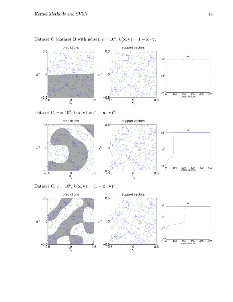
Kernel Methods and SVMs 10
If αj = 0 at the solution, then this means, informally speaking, that we didn’t really needto enforce this constraint at all: If we threw it out of the optimization, it would still “auto-matically” be obeyed. How could this be? Recall that the original optimization in Eq. 4.1 istrying to minimize all the zj . There are two things stopping it from flying down to −∞: theconstraint in Eq. 4.4 above, and the constraint that zj ≥ 0. If the constraint above can beremoved with out changing the solution, then it must be that zj = 0. Thus, αj = 0 impliesthat 1 − yjw · xj ≤ 0, or, equivalently, that
yjw · xj ≥ 1.
Thus non-support vectors are points that are very well classified, that are comfortably onthe right side of the linear boundary.
Now, imagine we take some xj with zj = 0, and remove it from the training set. It is prettyeasy to see that this is equivalent to taking the optimization
minz,w
c∑
i
zi +1
2||w||2
s.t. zi ≥ (1 − yiw · xi)
zi ≥ 0,
and just dropping the constraint that zj ≥ (1− yjw · xj), meaning that zj “decouples” fromthe other variables, and the optimization will pick zj = 0. But, as we saw above, this hasno effect. Thus, removing a non-support vector from the training set has no impact on theresulting classification rule.
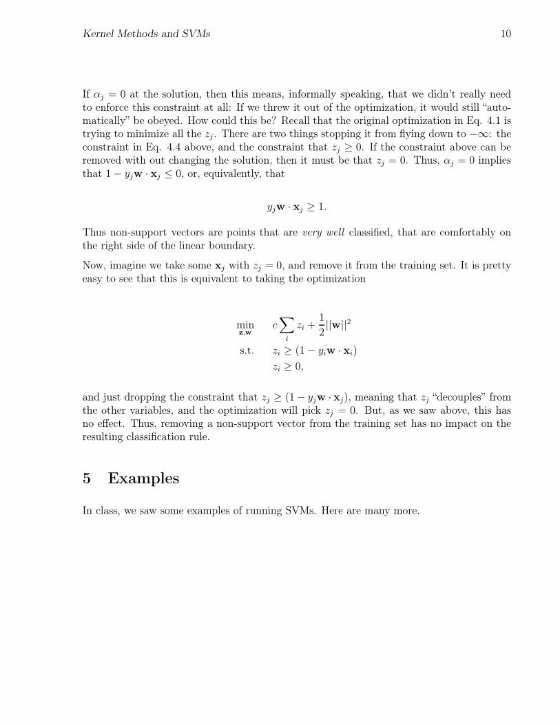
5 Examples
In class, we saw some examples of running SVMs. Here are many more.
Kernel Methods and SVMs 11
Dataset A, c = 10, k(x,v) = x · v.
−0.5 0 0.5−0.5
0
0.5
x1
x 2
predictions
−0.5 0 0.5−0.5
0
0.5
x1
x 2
support vectors
0 20 40 60 80 10010
−10
10−5
100
105
α
sorted indices
Dataset A, c = 103, k(x,v) = x · v.
−0.5 0 0.5−0.5
0
0.5
x1
x 2
predictions
−0.5 0 0.5−0.5
0
0.5
x1
x 2
support vectors
0 20 40 60 80 10010
−10
10−5
100
105
α
sorted indices
Dataset A, c = 105, k(x,v) = x · v.
−0.5 0 0.5−0.5
0
0.5
x1
x 2
predictions
−0.5 0 0.5−0.5
0
0.5
x1
x 2
support vectors
0 20 40 60 80 10010
−5
100
105
α
sorted indices

Kernel Methods and SVMs 12
Dataset A, c = 10, k(x,v) = 1 + x · v.
−0.5 0 0.5−0.5
0
0.5
x1
x 2
predictions
−0.5 0 0.5−0.5
0
0.5
x1
x 2
support vectors
0 20 40 60 80 10010
−15
10−10
10−5
100
105
α
sorted indices
Dataset A, c = 103, k(x,v) = 1 + x · v.
−0.5 0 0.5−0.5
0
0.5
x1
x 2
predictions
−0.5 0 0.5−0.5
0
0.5
x1
x 2
support vectors
0 20 40 60 80 10010
−10
10−5
100
105
α
sorted indices
Dataset A, c = 105, k(x,v) = 1 + x · v.
−0.5 0 0.5−0.5
0
0.5
x1
x 2
predictions
−0.5 0 0.5−0.5
0
0.5
x1
x 2
support vectors
0 20 40 60 80 10010
−10
10−5
100
105
α
sorted indices
Kernel Methods and SVMs 13
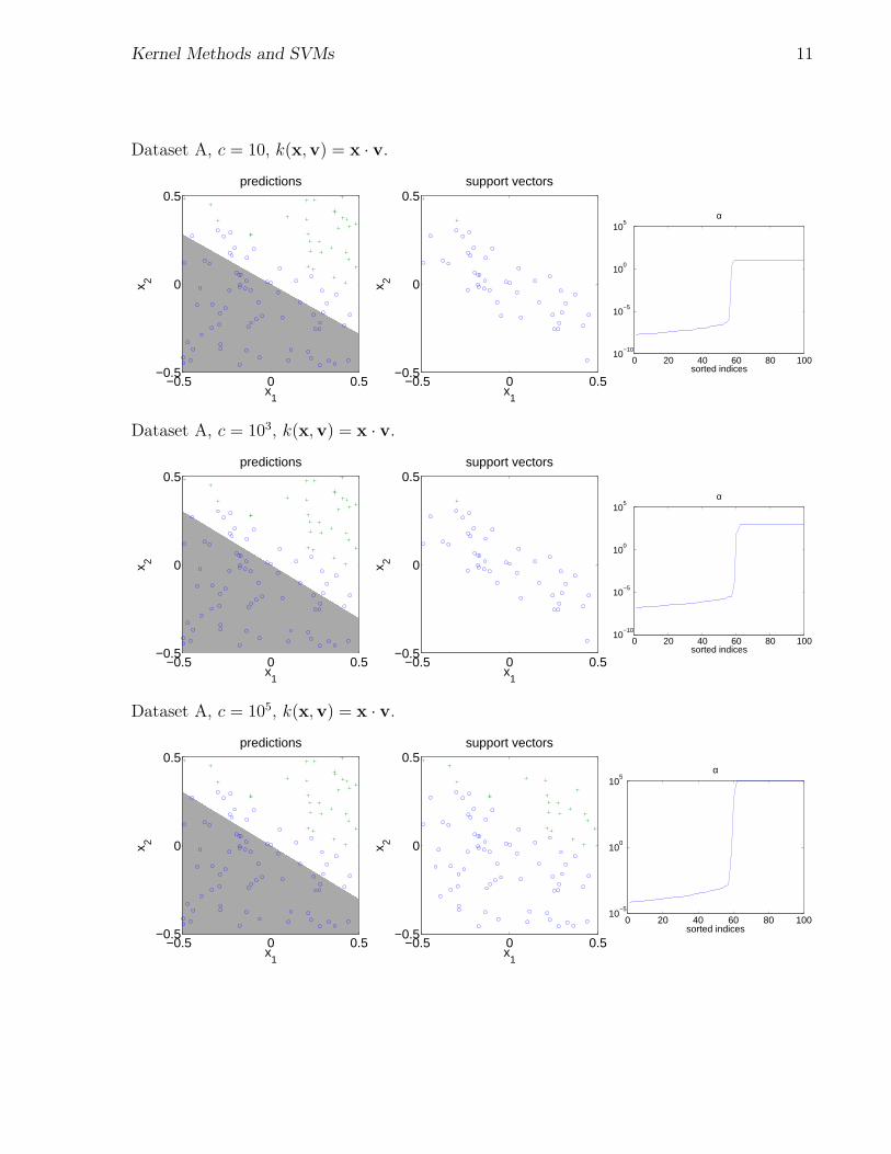
Dataset B, c = 105, k(x,v) = 1 + x · v.
−0.5 0 0.5−0.5
0
0.5
x1
x 2
predictions
−0.5 0 0.5−0.5
0
0.5
x1
x 2
support vectors
0 100 200 300 400 50010
−5
100
105
α
sorted indices
Dataset B, c = 105, k(x,v) = (1 + x · v)5.
−0.5 0 0.5−0.5
0
0.5
x1
x 2
predictions
−0.5 0 0.5−0.5
0
0.5
x1
x 2
support vectors
0 100 200 300 400 50010
−5
100
105
α
sorted indices
Dataset B, c = 105, k(x,v) = (1 + x · v)10.
−0.5 0 0.5−0.5
0
0.5
x1
x 2
predictions
−0.5 0 0.5−0.5
0
0.5
x1
x 2
support vectors
0 100 200 300 400 50010
−10
10−5
100
105
α
sorted indices
Kernel Methods and SVMs 14
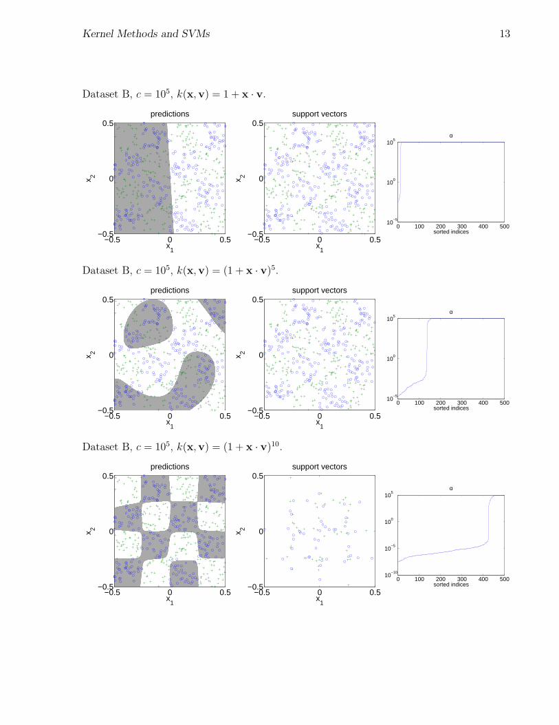
Dataset C (dataset B with noise), c = 105, k(x,v) = 1 + x · v.
−0.5 0 0.5−0.5
0
0.5
x1
x 2
predictions
−0.5 0 0.5−0.5
0
0.5
x1
x 2
support vectors
0 100 200 300 400 50010
−5
100
105
α
sorted indices
Dataset C, c = 105, k(x,v) = (1 + x · v)5.
−0.5 0 0.5−0.5
0
0.5
x1
x 2
predictions
−0.5 0 0.5−0.5
0
0.5
x1
x 2
support vectors
0 100 200 300 400 50010
−5
100
105
α
sorted indices
Dataset C, c = 105, k(x,v) = (1 + x · v)10.
−0.5 0 0.5−0.5
0
0.5
x1
x 2
predictions
−0.5 0 0.5−0.5
0
0.5
x1
x 2
support vectors
0 100 200 300 400 50010
−10
10−5
100
105
α
sorted indices
Kernel Methods and SVMs 15
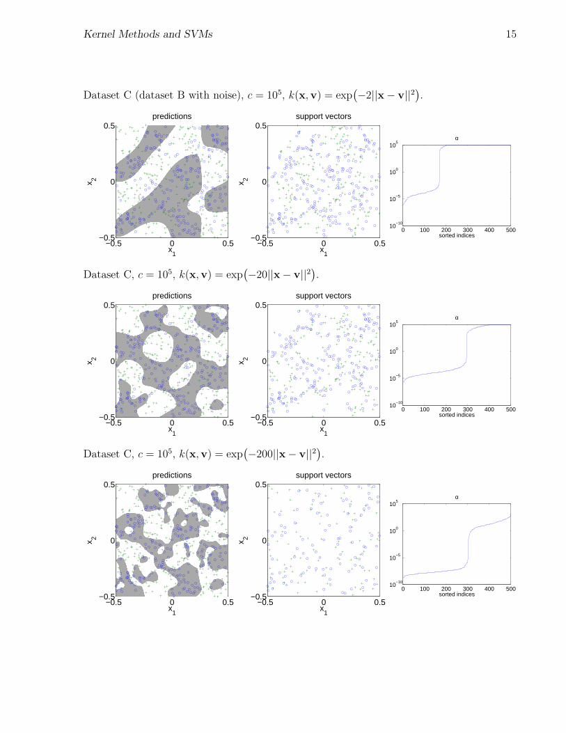
Dataset C (dataset B with noise), c = 105, k(x,v) = exp(
−2||x − v||2)
.
−0.5 0 0.5−0.5
0
0.5
x1
x 2
predictions
−0.5 0 0.5−0.5
0
0.5
x1
x 2
support vectors
0 100 200 300 400 50010
−10
10−5
100
105
α
sorted indices
Dataset C, c = 105, k(x,v) = exp(
−20||x − v||2)
.
−0.5 0 0.5−0.5
0
0.5
x1
x 2
predictions
−0.5 0 0.5−0.5
0
0.5
x1
x 2
support vectors
0 100 200 300 400 50010
−10
10−5
100
105
α
sorted indices
Dataset C, c = 105, k(x,v) = exp(
−200||x − v||2)
.
−0.5 0 0.5−0.5
0
0.5
x1
x 2
predictions
−0.5 0 0.5−0.5
0
0.5
x1
x 2
support vectors
0 100 200 300 400 50010
−10
10−5
100
105
α
sorted indices
Kernel Methods and SVMs 16
6 Kernel Theory
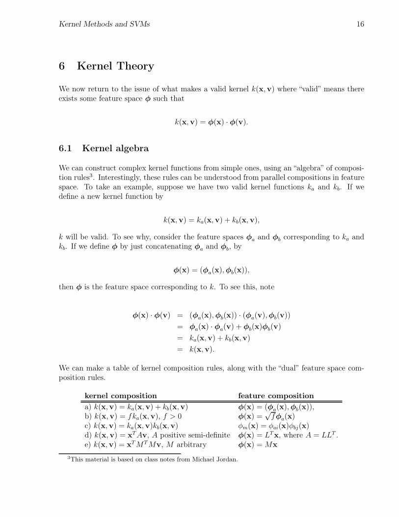
We now return to the issue of what makes a valid kernel k(x,v) where “valid” means thereexists some feature space φ such that
k(x,v) = φ(x) · φ(v).
6.1 Kernel algebra
We can construct complex kernel functions from simple ones, using an “algebra” of composi-tion rules3. Interestingly, these rules can be understood from parallel compositions in featurespace. To take an example, suppose we have two valid kernel functions ka and kb. If wedefine a new kernel function by
k(x,v) = ka(x,v) + kb(x,v),
k will be valid. To see why, consider the feature spaces φa and φb corresponding to ka andkb. If we define φ by just concatenating φa and φb, by
φ(x) = (φa(x), φb(x)),
then φ is the feature space corresponding to k. To see this, note
φ(x) · φ(v) = (φa(x), φb(x)) · (φa(v), φb(v))
= φa(x) · φa(v) + φb(x)φb(v)
= ka(x,v) + kb(x,v)
= k(x,v).
We can make a table of kernel composition rules, along with the “dual” feature space com-position rules.
kernel composition feature composition
a) k(x,v) = ka(x,v) + kb(x,v) φ(x) = (φa(x), φb(x)),b) k(x,v) = fka(x,v), f > 0 φ(x) =
√fφa(x)
c) k(x,v) = ka(x,v)kb(x,v) φm(x) = φai(x)φbj(x)d) k(x,v) = xT Av, A positive semi-definite φ(x) = LTx, where A = LLT .e) k(x,v) = xT MT Mv, M arbitrary φ(x) = Mx
3This material is based on class notes from Michael Jordan.

Kernel Methods and SVMs 17
We have already proven rule (a). Let’s prove some of the others.
Rule (b) is quite easy to understand:
φ(x) · φ(v) =√
fφa(x) ·√
fφa(v)
= fφa(x) · φa(v)
= fka(x,v)
= k(x,v)
Rule (c) is more complex. It is important to understand the notation. If
φa(x) = (φa1(x), φa2(x), φa3(x))
φb(x) = (φb1(x), φb2(x)),
then φ contains all six pairs.
φ(x) =(
φa1(x)φb1(x), φa2(x)φb1(x), φa3(x)φb1(x)
φa1(x)φb2(x), φa2(x)φb2(x), φa3(x)φb2(x))
With that understanding, we can prove rule (c) via
φ(x) · φ(v) =∑
m
φm(x)mφ(v)
=∑
i
∑
j
φai(x)φbj(x)φai(v)φbj(v)
=(
∑
i
φai(x)φai(v))(
∑
j
φbj(x)φbj(v))
=(
φa(x) · φa(v))(
φb(x) · φb(v))
= ka(x,v)kb(x,v)
= k(x,v).
Rule (d) follows from the well known result in linear algebra that a symmetric positivesemi-definite matrix A can be factored as A = LLT . With that known, clearly
Kernel Methods and SVMs 18
φ(x) · φ(v) = (Lx) · (Lv)
= xT LT Lv
= xT ATv
= xT Av
= k(x,v)
We can alternatively think of rule (d) as saying that k(x) = xT MT Mx corresponds to thebasis expansion φ(x) = Mx for any M . That gives rule (e).
6.2 Understanding Polynomial Kernels via Kernel Algebra
So, we have all these rules for combining kernels. What do they tell us? Rules (a),(b), and(c) essentially tell us that polynomial combinations of valid kernels are valid kernels. Usingthis, we can understand the meaning of polynomial kernels First off, for some scalar variablex, consider a polynomial kernel of the form
k(x, v) = (xv)d.
To what basis expansion does this kernel correspond? We can build this up stage by stage.
k(x, v) = xv ↔ φ(x) = (x)
k(x, v) = (xv)2 ↔ φ(x) = (x2) by rule (c)
k(x, v) = (xv)3 ↔ φ(x) = (x3) by rule (c).
If we work with vectors, we find that
k(x,v) = (x · v)
corresponds to φ(x) = x, while (by rule (c)) k(x,v) = (x ·v)2 corresponds to a feature spacewith all pairwise terms
φm(x) = xixj , 1 ≤ i, j ≤ n.
Similarly, k(x,v) = (x · v)3 corresponds to a feature space with all triplets
φm(x) = xixjxk, 1 ≤ i, j, k ≤ n.
Kernel Methods and SVMs 19
More generally, k(x,v) = (x · v)d corresponds to a feature space with terms
φm(x) = xi1xi2 ...xid , 1 ≤ ij ≤ n (6.1)
Thus, a polynomial kernel is equivalent to a polynomial basis expansion, with all terms oforder d. This is pretty surprising even though the word “polynomial” is in front of both ofthese terms! Again, we should reiterate the computational savings here. In general, comput-ing a polynomial basis expansion will take time O(nd). However, computing a polynomialkernel only takes time O(n). Again, though, we have only defeated the computational issuewith high-degree polynomial basis expansions. The statistical properties are unchanged.
Now, consider the kernel k(x,v) = (r + x · v)d. What is the impact of adding the constantof r? Notice that this is equivalent to simply taking the vectors x and v and prependinga constant of
√r to them. Thus, this kernel corresponds to a polynomial expansion with
constant terms added. One way to write this would be
φm(x) = xi1xi2 ...xid , 0 ≤ ij ≤ n (6.2)
where we consider x0 to be equal to√
r. Thus, this kernel is equivalent to a polynomial basisexpansion with all terms of all order less than or equal to d.
An interesting question is the impact of the constant r. Should we set it large or small? Whatis the impact of this choice. Notice that the lower-order terms in the basis expansion in Eq.6.2 will have many terms x0, and so get multiplied by a
√r to a high power. Meanwhile,
high order terms will have have few or no terms of x0, and so get multiplied by√
r to a lowpower. Thus, a large factor of r has the effect of making the low-order term larger, relativeto high-order terms.
Recall that if we make the basis expansion larger, this has the effect of reducing the theregularization penalty, since the same classification rule can be accomplished with a smallerweight. Thus, if we make part of a basis expansion larger, those parts of the basis expansionwill tend to play a larger role in the final classification rule. Thus, using a larger constant rhad the effect of making the low-order parts of the polynomial expansion in Eq. 6.2 tend tohave more impact.
6.3 Mercer’s Theorem
One thing we might worry about is if the SVM optimization is convex in α. The concern isif
∑
i
∑
j
αiαjyiyjk(xi,xj) (6.3)
Kernel Methods and SVMs 20
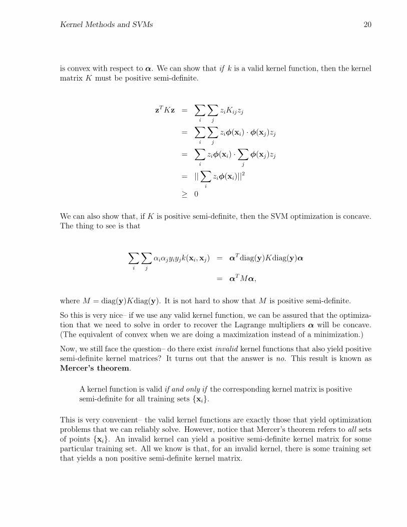
is convex with respect to α. We can show that if k is a valid kernel function, then the kernelmatrix K must be positive semi-definite.
zT Kz =∑
i
∑
j
ziKijzj
=∑
i
∑
j
ziφ(xi) · φ(xj)zj
=∑
i
ziφ(xi) ·∑
j
φ(xj)zj
= ||∑
i
ziφ(xi)||2
≥ 0
We can also show that, if K is positive semi-definite, then the SVM optimization is concave.The thing to see is that
∑
i
∑
j
αiαjyiyjk(xi,xj) = αT diag(y)Kdiag(y)α
= αT Mα,
where M = diag(y)Kdiag(y). It is not hard to show that M is positive semi-definite.
So this is very nice– if we use any valid kernel function, we can be assured that the optimiza-tion that we need to solve in order to recover the Lagrange multipliers α will be concave.(The equivalent of convex when we are doing a maximization instead of a minimization.)
Now, we still face the question– do there exist invalid kernel functions that also yield positivesemi-definite kernel matrices? It turns out that the answer is no. This result is known asMercer’s theorem.
A kernel function is valid if and only if the corresponding kernel matrix is positivesemi-definite for all training sets {xi}.
This is very convenient– the valid kernel functions are exactly those that yield optimizationproblems that we can reliably solve. However, notice that Mercer’s theorem refers to all setsof points {xi}. An invalid kernel can yield a positive semi-definite kernel matrix for someparticular training set. All we know is that, for an invalid kernel, there is some training setthat yields a non positive semi-definite kernel matrix.
Kernel Methods and SVMs 21
7 Our Story so Far
There were a lot of technical details here. It is worth taking a look back to do a conceptualoverview and make sure we haven’t missed the big picture. The starting point for SVMs isis minimizing the hinge loss under ridge regression, i.e.
w∗ = minw
c∑
i
(1 − yiw · xi)+ +1
2||w||2.
Fundamentally, SVMs are just fitting an optimization like this. The difference is that theyperform the optimization in a different way, and they allow you to work efficiently withpowerful basis expansions / kernel functions.
Act 1. We proved that if w∗ is the vector of weights that results from this optimization,then we could alternatively calculate w∗ as
w∗ =∑
i
αiyixi,
where the αi are given by the optimization
max0≤α≤c
∑
i
αi −1
2
∑
i
∑
j
αiαjyiyjxi · xj . (7.1)
With that optimization solved, we can classify a new point x by
f(x) = x ·w∗ =∑
i
αiyix · xi, (7.2)
Thus, if we want to, we can think of the variables αi as being the main things that we arefitting, rather than the weights w.
Act 2. Next, we noticed that the above optimization (Eq. 7.3) and classifier (Eq. 7.4)only depend on the inner products of the data elements. Thus, we could replace the innerproducts in these expressions with kernel evaluations, giving the optimization
max0≤α≤c
∑
i
αi −1
2
∑
i
∑
j
αiαjyiyjk(xi,xj), (7.3)
and the classification rule
Kernel Methods and SVMs 22
f(x) =∑
i
αiyik(x,xi), (7.4)
where k(x,v) = x · v.
Act 3. Now, imagine that instead of directly working with the data, we wanted to workwith some basis expansion. This would be easy to accomplish just by switching the kernelfunction to be
k(x,v) = φ(x) · φ(v).
However, we also noticed that for some basis expansions, like polynomials, we could computek(x,v) much more efficiently than explicitly forming the basis expansions and then takingthe inner product. We called this computational trick the “kernel trick”.
Act 4. Finally, we developed a “kernel algebra”, which allowed us to understand how wecan combine different kernel functions, and what this meant in feature space. We also sawMercer’s theorm, which tells us what kernel functions are and are not legal. Happily, thiscorresponded with the SVM optimization problem being convex.
8 Discussion
8.1 SVMs as Template Methods
Regardless of what we say, at the end of the day, support vector machines make theirpredictions through the classification rule
f(x) =∑
i
αiyik(x,xi).
Intuitively, k(x,xi) measures how “similar” x is to training example xi. This bears a strongresemblence to K-NN classification, where we use k as the distance metric, rather than some-thing like the Euclidean distance. Thus, SVMs can be seen as glorified template methods,where the amount that each point xi participates in predictions is reweighted in the learningstage. This is a view usually espoused by SVM skeptics, but a reasonable one. Remember,however, that there is absolutely nothing wrong with template methods.
Kernel Methods and SVMs 23
8.2 Theoretical Issues
An advantage of SVMs is that rigorous theoretical guarantees can often be given for theirperformance. It is possible to use these theoretical bounds to do model selection, ratherthan, e.g., cross validation. However, at the moment, these theoretical guarantees are ratherloose in practice, meaning that SVMs perform significantly better than the bounds can show.As such, one can often get better practical results by using more heuristic model selectionprocedures like cross validation. We will see this when we get to learning theory.