Santa Clara UniversityScholar Commons

Civil Engineering School of Engineering

6-7-2013

Errors in climate model daily precipitation andtemperature output: time invariance andimplications for bias correctionEdwin P. MaurerSanta Clara University, emaurer@scu.edu

Tapash Das

Daniel R. Cayan

Follow this and additional works at: https://scholarcommons.scu.edu/ceng

Part of the Civil and Environmental Engineering Commons

© Author(s) 2013. This work is distributed under the Creative Commons Attribution 3.0 License.

This Article is brought to you for free and open access by the School of Engineering at Scholar Commons. It has been accepted for inclusion in CivilEngineering by an authorized administrator of Scholar Commons. For more information, please contact rscroggin@scu.edu.

Recommended CitationMaurer, E.P., T. Das, and D.R. Cayan, 2013, Errors in climate model daily precipitation and temperature output: time invariance andimplications for bias correction, Hydrology and Earth System Sciences, 17, 2147-2159, doi:10.5194/hess-17-2147-2013.

Hydrol. Earth Syst. Sci., 17, 2147–2159, 2013www.hydrol-earth-syst-sci.net/17/2147/2013/doi:10.5194/hess-17-2147-2013© Author(s) 2013. CC Attribution 3.0 License.

EGU Journal Logos (RGB)

Advances in Geosciences

Open A

ccess

Natural Hazards and Earth System

Sciences

Open A

ccess

Annales Geophysicae

Open A

ccess

Nonlinear Processes in Geophysics

Open A

ccess

Atmospheric Chemistry

and Physics

Open A

ccess

Atmospheric Chemistry

and Physics

Open A

ccess

Discussions

Atmospheric Measurement

Techniques

Open A

ccess

Atmospheric Measurement

Techniques

Open A

ccess

Discussions

Biogeosciences

Open A

ccess

Open A

ccess

BiogeosciencesDiscussions

Climate of the Past

Open A

ccess

Open A

ccess

Climate of the Past

Discussions

Earth System Dynamics

Open A

ccess

Open A

ccess

Earth System Dynamics

Discussions

GeoscientificInstrumentation

Methods andData Systems

Open A

ccess

GeoscientificInstrumentation

Methods andData Systems

Open A

ccess

Discussions

GeoscientificModel Development

Open A

ccess

Open A

ccess

GeoscientificModel Development

Discussions

Hydrology and Earth System

SciencesO

pen Access

Hydrology and Earth System

Sciences

Open A

ccess

Discussions

Ocean Science

Open A

ccess

Open A

ccess

Ocean ScienceDiscussions

Solid Earth

Open A

ccess

Open A

ccess

Solid EarthDiscussions

The Cryosphere

Open A

ccess

Open A

ccess

The CryosphereDiscussions

Natural Hazards and Earth System

Sciences

Open A

ccess

Discussions

Errors in climate model daily precipitation and temperature output:time invariance and implications for bias correction

E. P. Maurer1, T. Das2, and D. R. Cayan3

1Civil Engineering Dept., Santa Clara University, Santa Clara, CA, USA2CH2MHill, 402 W. Broadway, San Diego, CA, USA3Division of Climate, Atmospheric Sciences, and Physical Oceanography, Scripps Institution of Oceanographyand Water Resources Division, US Geological Survey, La Jolla, CA, USA

Correspondence to:E. P. Maurer (emaurer@engr.scu.edu)

Received: 21 December 2012 – Published in Hydrol. Earth Syst. Sci. Discuss.: 1 February 2013Revised: 7 May 2013 – Accepted: 12 May 2013 – Published: 7 June 2013

Abstract. When correcting for biases in general circulationmodel (GCM) output, for example when statistically down-scaling for regional and local impacts studies, a common as-sumption is that the GCM biases can be characterized bycomparing model simulations and observations for a histor-ical period. We demonstrate some complications in this as-sumption, with GCM biases varying between mean and ex-treme values and for different sets of historical years. Dailyprecipitation and maximum and minimum temperature fromlate 20th century simulations by four GCMs over the UnitedStates were compared to gridded observations. Using randomyears from the historical record we select a “base” set and a10 yr independent “projected” set. We compare differences inbiases between these sets at median and extreme percentiles.On average a base set with as few as 4 randomly-selectedyears is often adequate to characterize the biases in dailyGCM precipitation and temperature, at both median and ex-treme values; 12 yr provided higher confidence that bias cor-rection would be successful. This suggests that some of theGCM bias is time invariant. When characterizing bias with aset of consecutive years, the set must be long enough to ac-commodate regional low frequency variability, since the biasalso exhibits this variability. Newer climate models includedin the Intergovernmental Panel on Climate Change fifth as-sessment will allow extending this study for a longer obser-vational period and to finer scales.

1 Introduction

The prospect of continued and intensifying climate changehas motivated the assessment of impacts at the local to re-gional scale, which entails the prerequisite use of down-scaling methods to translate large-scale general circulationmodel (GCM) output to a regionally relevant scale (Carter etal., 2007; Christensen et al., 2007). This downscaling is typ-ically categorized into two types: dynamical, using a higherresolution climate model that better represents the finer-scaleprocesses and terrain in the region of interest; and statisti-cal, where relationships are developed between large-scaleclimate statistics and those at a fine scale (Fowler et al.,2007). While dynamical downscaling has the advantage ofproducing complete, physically consistent fields, its com-putational demands preclude its common use when usingmultiple GCMs in a climate change impact assessment. Wethus focus our attention on statistical downscaling, and morespecifically on the bias correction inherently included in it.

With the development of coordinated GCM output, withstandardized experiments, formats, and archiving (Meehl etal., 2007), impact assessments can more readily use an en-semble of output from multiple GCMs. This allows the sepa-ration of various sources of uncertainties and the assessmentto some degree of the uncertainty due to GCM representationof climate sensitivity (Hawkins and Sutton, 2009; Knutti etal., 2008; Wehner, 2010). In combining a selection of GCMsto form an ensemble, the inherent errors in each GCM mustbe accommodated. In the ideal case, if all GCM biases werestationary in time (and with projected trends in the future),

Published by Copernicus Publications on behalf of the European Geosciences Union.

2148 E. P. Maurer et al.: Errors in climate model daily precipitation and temperature output

removing the bias during an observed period and applyingthe same bias correction into the future should produce aprojection into the future with lower bias as well. Ultimatelythis would place all GCM projections on a more or less equalfooting.

Some past studies support the assumption of time-invariant GCM biases in bias correction schemes. For ex-ample, Macadam et al. (2010), who demonstrate that usingGCM abilities to reproduce near-surface temperature anoma-lies (where biases in mean state are removed) was found toproduce inconsistent rankings (from best to worst) of GCMsfor different 20 yr periods in the 20th century. However,Macadam et al. (2010) found when actual temperatures wereused to assess model performance, a more stable GCM rank-ing was produced. While studying regional climate modelbiases, Christensen et al. (2008) found systematic biases inprecipitation and temperature related to observed mean val-ues, although the biases between different subsets of yearsincreased when they differed in temperature by 4–6◦C.

Biases in GCM output have been attributed to various cli-mate model deficiencies such as the coarse representation ofterrain (Masson and Knutti, 2011), cloud and convective pre-cipitation parameterization (Sun et al., 2006), surface albedofeedback (Randall et al., 2007), and representation of land-atmosphere interactions (Haerter et al., 2011) for example.Some of these deficiencies, as persistent model characteris-tics, would be expected to result in biases in the GCM outputthat are similar during different historical periods and intothe future. For example, errors in GCM simulations of tem-perature occur in regions of sharp elevation changes that arenot captured by the coarse GCM spatial scale (Randall et al.,2007); these errors would be expected to be evident to somedegree in model simulations for any time period. However, asHaerter et al. (2011) state “. . . bias correction cannot correctfor incorrect representations of dynamical and/or physicalprocesses . . . ”, which points toward the issue of some GCMdeficiencies producing different biases in land surface vari-ables as the climate warms, generically referred to as time-and state-dependent biases (Buser et al., 2009; Ehret et al.,2012). For example, Hall et al. (2008) show that biases inthe representation of spring snow albedo feedback in a GCMcan modify the summer temperature change sensitivity. Thisimplies that as global temperatures climb in future decades,some biases could be amplified by this feedback process.While we do not assess the sources of GCM biases explic-itly, we aim to examine where different GCMs exhibit simi-lar precipitation and temperature biases between two sets ofindependent years, which may carry implications as to whichsources of error are important in different regions.

Many of the prior assessments of GCM bias have beenbased on GCM simulations of monthly, seasonal, or an-nual mean quantities. Recognizing the important role of ex-treme events in the projected impacts of climate change(Christensen et al., 2007), statistical downscaling of dailyGCM output can been used to provide information on the

projected changes in regional extremes (e.g., Burger et al.,2012; Fowler et al., 2007; Tryhorn and DeGaetano, 2011).While accounting for biases at longer timescales, such asmonthly, can reduce the bias in daily GCM output, the dailyvariability of GCM output may have biases (such as exces-sive drizzle; e.g., Piani et al., 2010) that cannot be addressedby a correction at longer timescales. By addressing biases atthe daily scale, we can assess the ability to correct for biasesat a timescale appropriate for many extreme events (Frich etal., 2002).

Biases in daily GCM output can be removed in manyways. At its simplest, the perturbation, or “delta” methodshifts the observed mean by the GCM simulated meanchange, effectively accounting for GCM mean bias only(Hewitson, 2003), which is useful but has its limitations(Ballester et al., 2010). Separate perturbations can be appliedto different magnitude events (e.g., Vicuna et al., 2010) tocapture some of the potentially asymmetric biases in differ-ent portions of the observed probability distribution function.In its limit, perturbations can be applied along a continu-ous distribution, resulting in a quantile mapping technique(Maraun et al., 2010; Panofsky and Brier, 1968). This typeof approach has been applied in a variety of formulationsfor bias correcting monthly and daily climate model outputs(e.g., Abatzoglou and Brown, 2012; Boe et al., 2007; Inesand Hansen, 2006; Li et al., 2010; Piani et al., 2010; Themeßlet al., 2012; Thrasher et al., 2012), and has been shown tocompare favorably to other statistical bias correction meth-ods (Lafon et al., 2012). Regardless of the approach, all ofthese methods of bias removal assume that biases relative tohistoric observations will be the same during the projections.

For this study, we examine the biases in daily GCM out-put over the conterminous United States. We address the fol-lowing questions: (1) are the daily biases the same betweenmedian and extreme values? (2) Are biases the same overdifferent randomly selected sets of years (i.e., time invari-ant)? We address these using daily output from four GCMsfor precipitation, and maximum and minimum daily temper-ature. We consider biases at both median and extreme valuesbecause, as attention focuses on extreme events such as heatwaves, peak energy demand, and floods, the assumptions inbias correction of daily data at these extremes becomes atleast as important as at mean conditions.

2 Methods and data

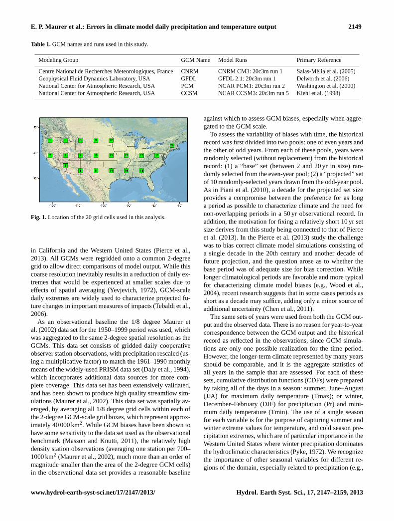
The domain used for this study is the conterminous UnitedStates, as represented by 20 individual 2◦ by 2◦ (lati-tude/longitude) grid boxes, shown in Fig. 1. For the pe-riod 1950–1999, daily precipitation, maximum and mini-mum temperature output were obtained from simulationsof four GCMs listed in Table 1. These four GCM runswere those selected for a wider project aimed at comparingdifferent statistical and dynamical downscaling techniques

Hydrol. Earth Syst. Sci., 17, 2147–2159, 2013 www.hydrol-earth-syst-sci.net/17/2147/2013/

E. P. Maurer et al.: Errors in climate model daily precipitation and temperature output 2149

Table 1.GCM names and runs used in this study.

Modeling Group GCM Name Model Runs Primary Reference

Centre National de Recherches Meteorologiques, France CNRM CNRM CM3: 20c3m run 1 Salas-Melia et al. (2005)Geophysical Fluid Dynamics Laboratory, USA GFDL GFDL 2.1: 20c3m run 1 Delworth et al. (2006)National Center for Atmospheric Research, USA PCM NCAR PCM1: 20c3m run 2 Washington et al. (2000)National Center for Atmospheric Research, USA CCSM NCAR CCSM3: 20c3m run 5 Kiehl et al. (1998)

Fig. 1.Location of the 20 grid cells used in this analysis.

in California and the Western United States (Pierce et al.,2013). All GCMs were regridded onto a common 2-degreegrid to allow direct comparisons of model output. While thiscoarse resolution inevitably results in a reduction of daily ex-tremes that would be experienced at smaller scales due toeffects of spatial averaging (Yevjevich, 1972), GCM-scaledaily extremes are widely used to characterize projected fu-ture changes in important measures of impacts (Tebaldi et al.,2006).

As an observational baseline the 1/8 degree Maurer etal. (2002) data set for the 1950–1999 period was used, whichwas aggregated to the same 2-degree spatial resolution as theGCMs. This data set consists of gridded daily cooperativeobserver station observations, with precipitation rescaled (us-ing a multiplicative factor) to match the 1961–1990 monthlymeans of the widely-used PRISM data set (Daly et al., 1994),which incorporates additional data sources for more com-plete coverage. This data set has been extensively validated,and has been shown to produce high quality streamflow sim-ulations (Maurer et al., 2002). This data set was spatially av-eraged, by averaging all 1/8 degree grid cells within each ofthe 2-degree GCM-scale grid boxes, which represent approx-imately 40 000 km2. While GCM biases have been shown tohave some sensitivity to the data set used as the observationalbenchmark (Masson and Knutti, 2011), the relatively highdensity station observations (averaging one station per 700–1000 km2 (Maurer et al., 2002), much more than an order ofmagnitude smaller than the area of the 2-degree GCM cells)in the observational data set provides a reasonable baseline

against which to assess GCM biases, especially when aggre-gated to the GCM scale.

To assess the variability of biases with time, the historicalrecord was first divided into two pools: one of even years andthe other of odd years. From each of these pools, years wererandomly selected (without replacement) from the historicalrecord: (1) a “base” set (between 2 and 20 yr in size) ran-domly selected from the even-year pool; (2) a “projected” setof 10 randomly-selected years drawn from the odd-year pool.As in Piani et al. (2010), a decade for the projected set sizeprovides a compromise between the preference for as longa period as possible to characterize climate and the need fornon-overlapping periods in a 50 yr observational record. Inaddition, the motivation for fixing a relatively short 10 yr setsize derives from this study being connected to that of Pierceet al. (2013). In the Pierce et al. (2013) study the challengewas to bias correct climate model simulations consisting ofa single decade in the 20th century and another decade offuture projection, and the question arose as to whether thebase period was of adequate size for bias correction. Whilelonger climatological periods are favorable and more typicalfor characterizing climate model biases (e.g., Wood et al.,2004), recent research suggests that in some cases periods asshort as a decade may suffice, adding only a minor source ofadditional uncertainty (Chen et al., 2011).

The same sets of years were used from both the GCM out-put and the observed data. There is no reason for year-to-yearcorrespondence between the GCM output and the historicalrecord as reflected in the observations, since GCM simula-tions are only one possible realization for the time period.However, the longer-term climate represented by many yearsshould be comparable, and it is the aggregate statistics ofall years in the sample that are assessed. For each of thesesets, cumulative distribution functions (CDFs) were preparedby taking all of the days in a season: summer, June–August(JJA) for maximum daily temperature (Tmax); or winter,December–February (DJF) for precipitation (Pr) and mini-mum daily temperature (Tmin). The use of a single seasonfor each variable is for the purpose of capturing summer andwinter extreme values for temperature, and cold season pre-cipitation extremes, which are of particular importance in theWestern United States where winter precipitation dominatesthe hydroclimatic characteristics (Pyke, 1972). We recognizethe importance of other seasonal variables for different re-gions of the domain, especially related to precipitation (e.g.,

www.hydrol-earth-syst-sci.net/17/2147/2013/ Hydrol. Earth Syst. Sci., 17, 2147–2159, 2013

2150 E. P. Maurer et al.: Errors in climate model daily precipitation and temperature output

Karl et al., 2009), but reserve a more comprehensive effortfor future research. Within each season, two percentiles areselected for analysis: the median and the 95th percentile forPr and Tmax, and the median and 5th percentile for Tmin.

A Monte Carlo experiment was performed by repeating100 times the random selection of “base” sets and 10 yr “pro-jected” sets. This number of simulations was chosen to pro-vide adequate (so that repeated computations produced com-parable results) sampling for all selections of sets of yearswithout approaching the maximum number of combinationsfor the most limiting case, that is, 300 possible combinationsof 2 yr selected from a pool of 25 yr. Also, a second set of 100Monte Carlo simulations was performed, which produced in-distinguishable results, showing this number of simulationsis adequate for producing consistent results. For each of thebase and projected sets, the constructed CDFs were used todetermine the 50th and 95th (Tmax and Pr) or 5th and 50th(Tmin) percentiles for both observations and GCM output.The GCM biases relative to observations were calculated,composing two arrays of 100 values at each percentile.

At each percentile and for each Monte Carlo simulation,the samples are compared using the followingR index:

R =|BP− BB|

(|BP| + |BB|)/

2(1)

whereB is the bias, the difference between the GCM valueand the observed value, and the subscripts “P” and “B” in-dicate the projected and base sets, respectively; the verticalbars are the absolute value operator. What this index repre-sents is the ratio of the difference in bias between the baseand projected sets and the average bias of the base and pro-jected sets. A value ofR greater than one indicates a largerdifference in bias between the two sets than the average biasof the GCM, meaning a higher likelihood that bias correctionwould degrade the GCM output rather than improve it.R hasa range of 0≤ R ≤ 2. This index is similar to that used byMaraun (2012) to characterize the effectiveness of bias cor-rection of temperatures produced by regional climate mod-els. The principal difference in theR index to that of Ma-raun (2012) is that theR index is normalized by an estimateof the mean bias; since in this case both the base and pro-jected sets are selected from the historical record, the meanof the two bias estimates (for the base and projected sets) isused to estimate the average bias. The above procedure is re-peated at each of the 20 selected grid cells and for the fourGCMs included in this analysis.

As an alternative, the mean bias in the denominator couldbe estimated differently, such as using only the base periodbias BB. The advantage of using theR formulation aboveis that it is insensitive to which set is designated as “pro-jected” and which is “base”. For example,BB = 4, BP = 2andBB = 2, BP = 4 produce the sameR value, but wouldnot if only BB or BP were used in the denominator. This pro-vides the additional advantage that, since both the base andprojected sets are randomly drawn from the historical record

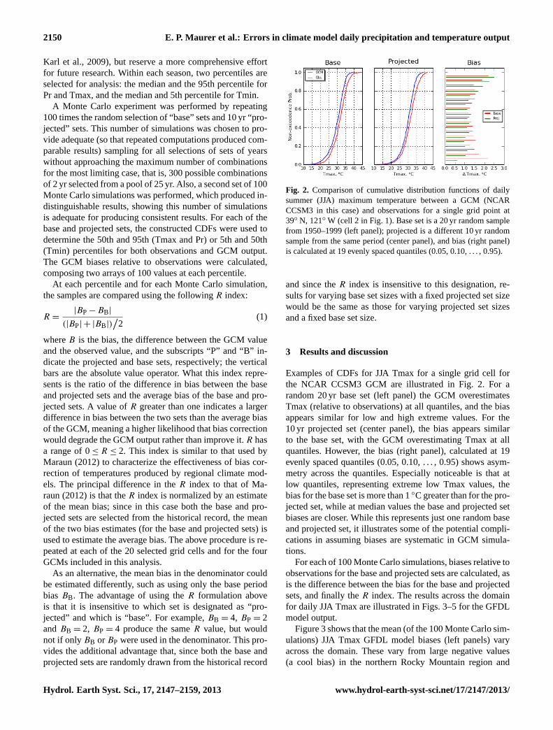
Fig. 2. Comparison of cumulative distribution functions of dailysummer (JJA) maximum temperature between a GCM (NCARCCSM3 in this case) and observations for a single grid point at39◦ N, 121◦ W (cell 2 in Fig. 1). Base set is a 20 yr random samplefrom 1950–1999 (left panel); projected is a different 10 yr randomsample from the same period (center panel), and bias (right panel)is calculated at 19 evenly spaced quantiles (0.05, 0.10, . . . , 0.95).

and since theR index is insensitive to this designation, re-sults for varying base set sizes with a fixed projected set sizewould be the same as those for varying projected set sizesand a fixed base set size.

3 Results and discussion

Examples of CDFs for JJA Tmax for a single grid cell forthe NCAR CCSM3 GCM are illustrated in Fig. 2. For arandom 20 yr base set (left panel) the GCM overestimatesTmax (relative to observations) at all quantiles, and the biasappears similar for low and high extreme values. For the10 yr projected set (center panel), the bias appears similarto the base set, with the GCM overestimating Tmax at allquantiles. However, the bias (right panel), calculated at 19evenly spaced quantiles (0.05, 0.10, . . . , 0.95) shows asym-metry across the quantiles. Especially noticeable is that atlow quantiles, representing extreme low Tmax values, thebias for the base set is more than 1◦C greater than for the pro-jected set, while at median values the base and projected setbiases are closer. While this represents just one random baseand projected set, it illustrates some of the potential compli-cations in assuming biases are systematic in GCM simula-tions.

For each of 100 Monte Carlo simulations, biases relative toobservations for the base and projected sets are calculated, asis the difference between the bias for the base and projectedsets, and finally theR index. The results across the domainfor daily JJA Tmax are illustrated in Figs. 3–5 for the GFDLmodel output.

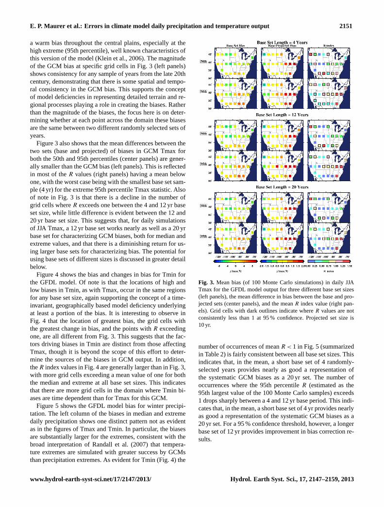
Figure 3 shows that the mean (of the 100 Monte Carlo sim-ulations) JJA Tmax GFDL model biases (left panels) varyacross the domain. These vary from large negative values(a cool bias) in the northern Rocky Mountain region and

Hydrol. Earth Syst. Sci., 17, 2147–2159, 2013 www.hydrol-earth-syst-sci.net/17/2147/2013/

E. P. Maurer et al.: Errors in climate model daily precipitation and temperature output 2151

a warm bias throughout the central plains, especially at thehigh extreme (95th percentile), well known characteristics ofthis version of the model (Klein et al., 2006). The magnitudeof the GCM bias at specific grid cells in Fig. 3 (left panels)shows consistency for any sample of years from the late 20thcentury, demonstrating that there is some spatial and tempo-ral consistency in the GCM bias. This supports the conceptof model deficiencies in representing detailed terrain and re-gional processes playing a role in creating the biases. Ratherthan the magnitude of the biases, the focus here is on deter-mining whether at each point across the domain these biasesare the same between two different randomly selected sets ofyears.

Figure 3 also shows that the mean differences between thetwo sets (base and projected) of biases in GCM Tmax forboth the 50th and 95th percentiles (center panels) are gener-ally smaller than the GCM bias (left panels). This is reflectedin most of theR values (right panels) having a mean belowone, with the worst case being with the smallest base set sam-ple (4 yr) for the extreme 95th percentile Tmax statistic. Alsoof note in Fig. 3 is that there is a decline in the number ofgrid cells whereR exceeds one between the 4 and 12 yr baseset size, while little difference is evident between the 12 and20 yr base set size. This suggests that, for daily simulationsof JJA Tmax, a 12 yr base set works nearly as well as a 20 yrbase set for characterizing GCM biases, both for median andextreme values, and that there is a diminishing return for us-ing larger base sets for characterizing bias. The potential forusing base sets of different sizes is discussed in greater detailbelow.

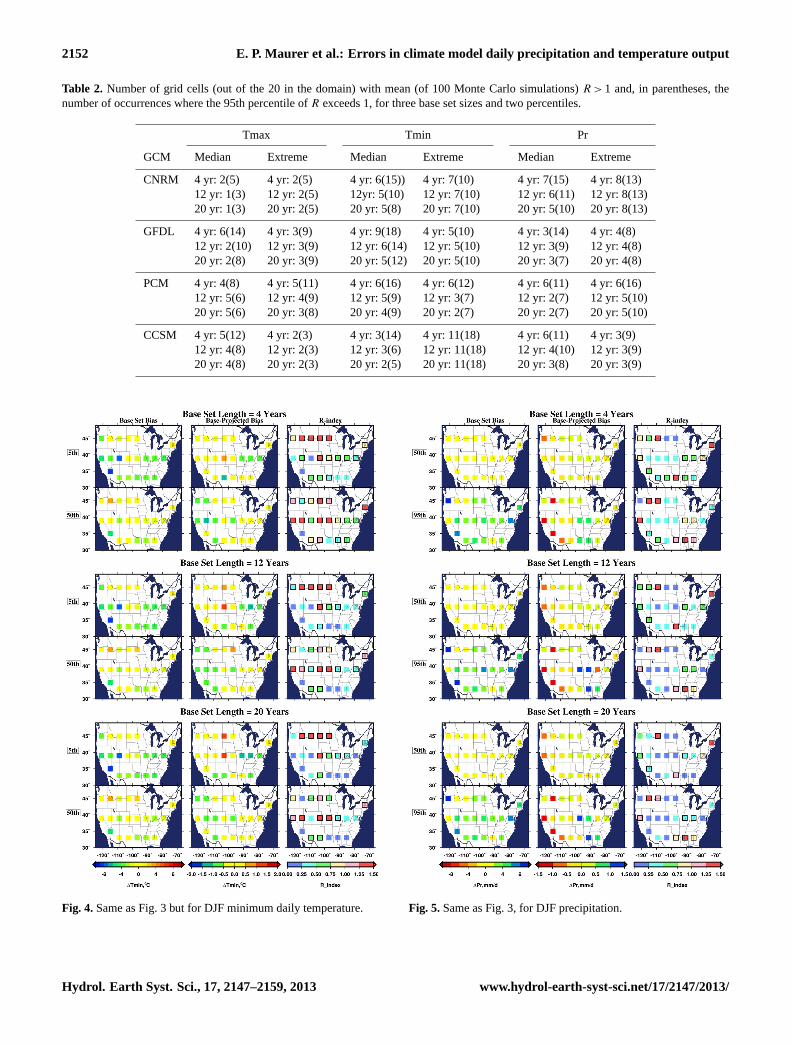
Figure 4 shows the bias and changes in bias for Tmin forthe GFDL model. Of note is that the locations of high andlow biases in Tmin, as with Tmax, occur in the same regionsfor any base set size, again supporting the concept of a time-invariant, geographically based model deficiency underlyingat least a portion of the bias. It is interesting to observe inFig. 4 that the location of greatest bias, the grid cells withthe greatest change in bias, and the points withR exceedingone, are all different from Fig. 3. This suggests that the fac-tors driving biases in Tmin are distinct from those affectingTmax, though it is beyond the scope of this effort to deter-mine the sources of the biases in GCM output. In addition,theR index values in Fig. 4 are generally larger than in Fig. 3,with more grid cells exceeding a mean value of one for boththe median and extreme at all base set sizes. This indicatesthat there are more grid cells in the domain where Tmin bi-ases are time dependent than for Tmax for this GCM.

Figure 5 shows the GFDL model bias for winter precipi-tation. The left column of the biases in median and extremedaily precipitation shows one distinct pattern not as evidentas in the figures of Tmax and Tmin. In particular, the biasesare substantially larger for the extremes, consistent with thebroad interpretation of Randall et al. (2007) that tempera-ture extremes are simulated with greater success by GCMsthan precipitation extremes. As evident for Tmin (Fig. 4) the

Fig. 3. Mean bias (of 100 Monte Carlo simulations) in daily JJATmax for the GFDL model output for three different base set sizes(left panels), the mean difference in bias between the base and pro-jected sets (center panels), and the meanR index value (right pan-els). Grid cells with dark outlines indicate whereR values are notconsistently less than 1 at 95 % confidence. Projected set size is10 yr.

number of occurrences of meanR < 1 in Fig. 5 (summarizedin Table 2) is fairly consistent between all base set sizes. Thisindicates that, in the mean, a short base set of 4 randomly-selected years provides nearly as good a representation ofthe systematic GCM biases as a 20 yr set. The number ofoccurrences where the 95th percentileR (estimated as the95th largest value of the 100 Monte Carlo samples) exceeds1 drops sharply between a 4 and 12 yr base period. This indi-cates that, in the mean, a short base set of 4 yr provides nearlyas good a representation of the systematic GCM biases as a20 yr set. For a 95 % confidence threshold, however, a longerbase set of 12 yr provides improvement in bias correction re-sults.

www.hydrol-earth-syst-sci.net/17/2147/2013/ Hydrol. Earth Syst. Sci., 17, 2147–2159, 2013

2152 E. P. Maurer et al.: Errors in climate model daily precipitation and temperature output

Table 2. Number of grid cells (out of the 20 in the domain) with mean (of 100 Monte Carlo simulations)R > 1 and, in parentheses, thenumber of occurrences where the 95th percentile ofR exceeds 1, for three base set sizes and two percentiles.

Tmax Tmin Pr

GCM Median Extreme Median Extreme Median Extreme

CNRM 4 yr: 2(5) 4 yr: 2(5) 4 yr: 6(15)) 4 yr: 7(10) 4 yr: 7(15) 4 yr: 8(13)12 yr: 1(3) 12 yr: 2(5) 12yr: 5(10) 12 yr: 7(10) 12 yr: 6(11) 12 yr: 8(13)20 yr: 1(3) 20 yr: 2(5) 20 yr: 5(8) 20 yr: 7(10) 20 yr: 5(10) 20 yr: 8(13)

GFDL 4 yr: 6(14) 4 yr: 3(9) 4 yr: 9(18) 4 yr: 5(10) 4 yr: 3(14) 4 yr: 4(8)12 yr: 2(10) 12 yr: 3(9) 12 yr: 6(14) 12 yr: 5(10) 12 yr: 3(9) 12 yr: 4(8)20 yr: 2(8) 20 yr: 3(9) 20 yr: 5(12) 20 yr: 5(10) 20 yr: 3(7) 20 yr: 4(8)

PCM 4 yr: 4(8) 4 yr: 5(11) 4 yr: 6(16) 4 yr: 6(12) 4 yr: 6(11) 4 yr: 6(16)12 yr: 5(6) 12 yr: 4(9) 12 yr: 5(9) 12 yr: 3(7) 12 yr: 2(7) 12 yr: 5(10)20 yr: 5(6) 20 yr: 3(8) 20 yr: 4(9) 20 yr: 2(7) 20 yr: 2(7) 20 yr: 5(10)

CCSM 4 yr: 5(12) 4 yr: 2(3) 4 yr: 3(14) 4 yr: 11(18) 4 yr: 6(11) 4 yr: 3(9)12 yr: 4(8) 12 yr: 2(3) 12 yr: 3(6) 12 yr: 11(18) 12 yr: 4(10) 12 yr: 3(9)20 yr: 4(8) 20 yr: 2(3) 20 yr: 2(5) 20 yr: 11(18) 20 yr: 3(8) 20 yr: 3(9)

Fig. 4.Same as Fig. 3 but for DJF minimum daily temperature. Fig. 5.Same as Fig. 3, for DJF precipitation.

Hydrol. Earth Syst. Sci., 17, 2147–2159, 2013 www.hydrol-earth-syst-sci.net/17/2147/2013/

E. P. Maurer et al.: Errors in climate model daily precipitation and temperature output 2153

Table 2 summarizes the right columns in Figs. 3, 4, and 5as well as the results for the other three GCMs included inthis study, to assess whether some of the same patterns ob-served for the GFDL model are shared across the four GCMs.Table 2 shows the pattern of larger base sets providing feweroccurrences ofR > 1. This is more evident between 4 yr and12 yr base sets; between 12 and 20 yr sets the results arebroadly similar. However, in many cases both median andextreme values show comparable numbers ofR > 1 occur-rences at all base set sizes, with the exceptions in only a fewcases (e.g., GFDL median Tmax and Tmin, and PCM andCCSM median Pr). This shows that for Tmax and Pr, in themean, bias correction would be successful in most cases us-ing base set sizes of only 4 randomly selected years. The sin-gle case where bias correction for more than half of the cellswould fail, ultimately worsening the bias, is CCSM extremeTmin, where 11 grid cells showR > 1 on average. For thiscase, even a 20 yr base set size does not alleviate the prob-lem. This suggests that if the bias cannot be characterizedwith a few years of daily data, it may lack adequate time in-variance to be amenable to this form of bias correction withany number of years constituting a base set. It is interestingthat this same model has the fewest number of occurrencesof R > 1 for median daily Tmin, and demonstrates success-ful bias correction even with a base set of 4 yr. Thus, differentprocesses are likely responsible for the CCSM model biasesin mean and extreme daily Tmin values.

The above discussion focused on grid cells where the meanR index exceeded one, in which case on average the bias cor-rection degrades the skill. To examine a more stringent stan-dard, Table 2 also summarizes the number of grid cells ineach case where the 95th percentileR values for each GCM,variable, and base set size, exceeds 1. This approximates thenumber of cells (outlined in Figs. 3–5) where a 95 % con-fidence thatR < 1 cannot be claimed. Of the 20 grid cellsanalyzed in this study, as many as 18 show theR < 1 hypoth-esis being rejected (CCSM extreme Tmin and GFDL medianTmin) and in other cases as few as 3 occurrences (CNRMmedian Tmax, CCSM extreme Tmax). While bias correctionhas a positive effect in the mean, the value ofR being belowone with a high confidence (95 %) is not strongly supported,especially for Tmin and Pr.

A final observation in Table 2 of the mean number of oc-currences ofR > 1 is that the GCM showing the fewest num-ber of cases varies for different variables, base set sizes, andwhether median or extreme statistics are considered. Sincethe relative rank among GCMs is not consistent across vari-ables, it can be concluded that among the models used in thisstudy no GCM can be broadly characterized as producingoutput that is more likely to benefit from statistical bias cor-rection than any other GCM. However, in the case where aspecific variable is of interest, some GCMs can clearly out-perform others. For example, for maximum temperatures theCNRM model demonstrates more time invariance in biasesthan the other GCMs. Thus, the apparent time invariance of

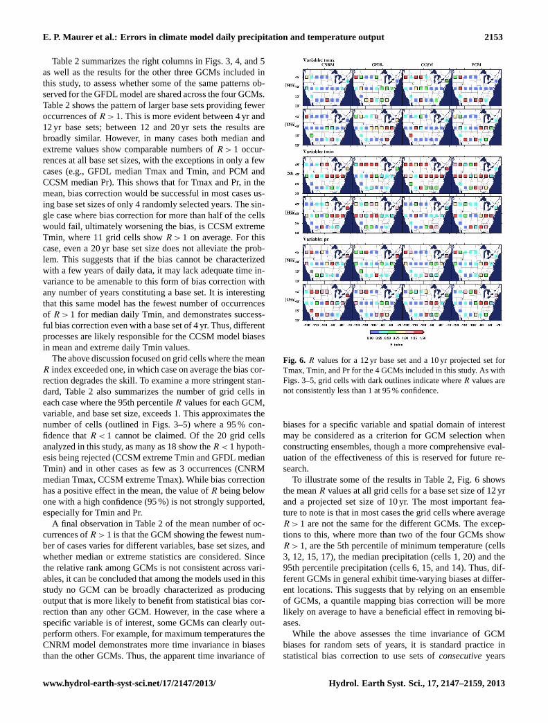
Fig. 6. R values for a 12 yr base set and a 10 yr projected set forTmax, Tmin, and Pr for the 4 GCMs included in this study. As withFigs. 3–5, grid cells with dark outlines indicate whereR values arenot consistently less than 1 at 95 % confidence.

biases for a specific variable and spatial domain of interestmay be considered as a criterion for GCM selection whenconstructing ensembles, though a more comprehensive eval-uation of the effectiveness of this is reserved for future re-search.

To illustrate some of the results in Table 2, Fig. 6 showsthe meanR values at all grid cells for a base set size of 12 yrand a projected set size of 10 yr. The most important fea-ture to note is that in most cases the grid cells where averageR > 1 are not the same for the different GCMs. The excep-tions to this, where more than two of the four GCMs showR > 1, are the 5th percentile of minimum temperature (cells3, 12, 15, 17), the median precipitation (cells 1, 20) and the95th percentile precipitation (cells 6, 15, and 14). Thus, dif-ferent GCMs in general exhibit time-varying biases at differ-ent locations. This suggests that by relying on an ensembleof GCMs, a quantile mapping bias correction will be morelikely on average to have a beneficial effect in removing bi-ases.

While the above assesses the time invariance of GCMbiases for random sets of years, it is standard practice instatistical bias correction to use sets ofconsecutiveyears

www.hydrol-earth-syst-sci.net/17/2147/2013/ Hydrol. Earth Syst. Sci., 17, 2147–2159, 2013

2154 E. P. Maurer et al.: Errors in climate model daily precipitation and temperature output

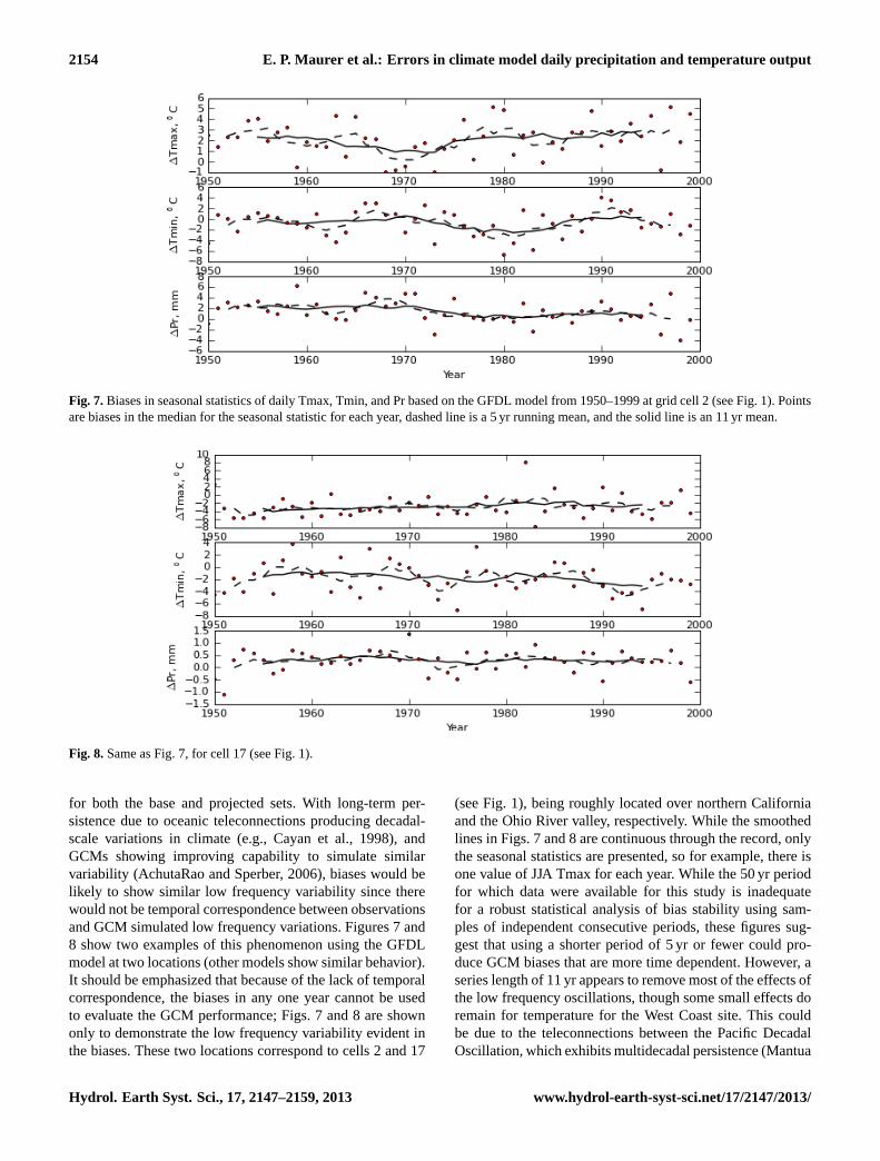
Fig. 7.Biases in seasonal statistics of daily Tmax, Tmin, and Pr based on the GFDL model from 1950–1999 at grid cell 2 (see Fig. 1). Pointsare biases in the median for the seasonal statistic for each year, dashed line is a 5 yr running mean, and the solid line is an 11 yr mean.

Fig. 8.Same as Fig. 7, for cell 17 (see Fig. 1).

for both the base and projected sets. With long-term per-sistence due to oceanic teleconnections producing decadal-scale variations in climate (e.g., Cayan et al., 1998), andGCMs showing improving capability to simulate similarvariability (AchutaRao and Sperber, 2006), biases would belikely to show similar low frequency variability since therewould not be temporal correspondence between observationsand GCM simulated low frequency variations. Figures 7 and8 show two examples of this phenomenon using the GFDLmodel at two locations (other models show similar behavior).It should be emphasized that because of the lack of temporalcorrespondence, the biases in any one year cannot be usedto evaluate the GCM performance; Figs. 7 and 8 are shownonly to demonstrate the low frequency variability evident inthe biases. These two locations correspond to cells 2 and 17

(see Fig. 1), being roughly located over northern Californiaand the Ohio River valley, respectively. While the smoothedlines in Figs. 7 and 8 are continuous through the record, onlythe seasonal statistics are presented, so for example, there isone value of JJA Tmax for each year. While the 50 yr periodfor which data were available for this study is inadequatefor a robust statistical analysis of bias stability using sam-ples of independent consecutive periods, these figures sug-gest that using a shorter period of 5 yr or fewer could pro-duce GCM biases that are more time dependent. However, aseries length of 11 yr appears to remove most of the effects ofthe low frequency oscillations, though some small effects doremain for temperature for the West Coast site. This couldbe due to the teleconnections between the Pacific DecadalOscillation, which exhibits multidecadal persistence (Mantua

Hydrol. Earth Syst. Sci., 17, 2147–2159, 2013 www.hydrol-earth-syst-sci.net/17/2147/2013/

E. P. Maurer et al.: Errors in climate model daily precipitation and temperature output 2155

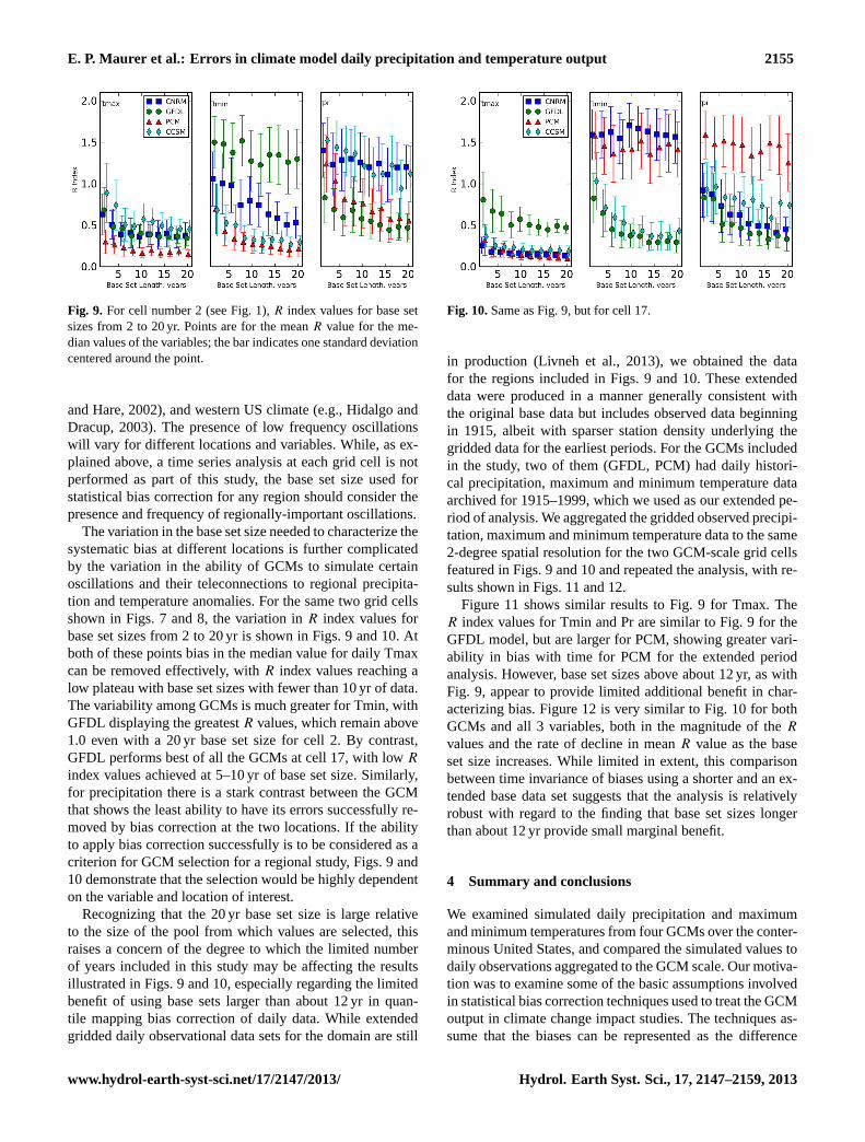
Fig. 9. For cell number 2 (see Fig. 1),R index values for base setsizes from 2 to 20 yr. Points are for the meanR value for the me-dian values of the variables; the bar indicates one standard deviationcentered around the point.

and Hare, 2002), and western US climate (e.g., Hidalgo andDracup, 2003). The presence of low frequency oscillationswill vary for different locations and variables. While, as ex-plained above, a time series analysis at each grid cell is notperformed as part of this study, the base set size used forstatistical bias correction for any region should consider thepresence and frequency of regionally-important oscillations.

The variation in the base set size needed to characterize thesystematic bias at different locations is further complicatedby the variation in the ability of GCMs to simulate certainoscillations and their teleconnections to regional precipita-tion and temperature anomalies. For the same two grid cellsshown in Figs. 7 and 8, the variation inR index values forbase set sizes from 2 to 20 yr is shown in Figs. 9 and 10. Atboth of these points bias in the median value for daily Tmaxcan be removed effectively, withR index values reaching alow plateau with base set sizes with fewer than 10 yr of data.The variability among GCMs is much greater for Tmin, withGFDL displaying the greatestR values, which remain above1.0 even with a 20 yr base set size for cell 2. By contrast,GFDL performs best of all the GCMs at cell 17, with lowRindex values achieved at 5–10 yr of base set size. Similarly,for precipitation there is a stark contrast between the GCMthat shows the least ability to have its errors successfully re-moved by bias correction at the two locations. If the abilityto apply bias correction successfully is to be considered as acriterion for GCM selection for a regional study, Figs. 9 and10 demonstrate that the selection would be highly dependenton the variable and location of interest.

Recognizing that the 20 yr base set size is large relativeto the size of the pool from which values are selected, thisraises a concern of the degree to which the limited numberof years included in this study may be affecting the resultsillustrated in Figs. 9 and 10, especially regarding the limitedbenefit of using base sets larger than about 12 yr in quan-tile mapping bias correction of daily data. While extendedgridded daily observational data sets for the domain are still

Fig. 10.Same as Fig. 9, but for cell 17.

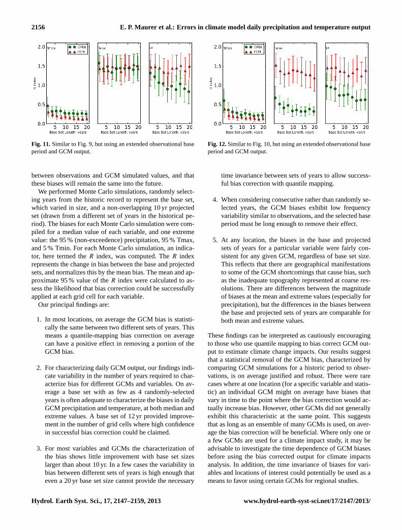
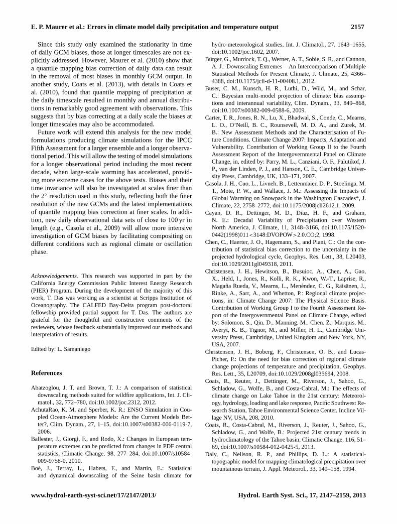
in production (Livneh et al., 2013), we obtained the datafor the regions included in Figs. 9 and 10. These extendeddata were produced in a manner generally consistent withthe original base data but includes observed data beginningin 1915, albeit with sparser station density underlying thegridded data for the earliest periods. For the GCMs includedin the study, two of them (GFDL, PCM) had daily histori-cal precipitation, maximum and minimum temperature dataarchived for 1915–1999, which we used as our extended pe-riod of analysis. We aggregated the gridded observed precipi-tation, maximum and minimum temperature data to the same2-degree spatial resolution for the two GCM-scale grid cellsfeatured in Figs. 9 and 10 and repeated the analysis, with re-sults shown in Figs. 11 and 12.

Figure 11 shows similar results to Fig. 9 for Tmax. TheR index values for Tmin and Pr are similar to Fig. 9 for theGFDL model, but are larger for PCM, showing greater vari-ability in bias with time for PCM for the extended periodanalysis. However, base set sizes above about 12 yr, as withFig. 9, appear to provide limited additional benefit in char-acterizing bias. Figure 12 is very similar to Fig. 10 for bothGCMs and all 3 variables, both in the magnitude of theR

values and the rate of decline in meanR value as the baseset size increases. While limited in extent, this comparisonbetween time invariance of biases using a shorter and an ex-tended base data set suggests that the analysis is relativelyrobust with regard to the finding that base set sizes longerthan about 12 yr provide small marginal benefit.

4 Summary and conclusions

We examined simulated daily precipitation and maximumand minimum temperatures from four GCMs over the conter-minous United States, and compared the simulated values todaily observations aggregated to the GCM scale. Our motiva-tion was to examine some of the basic assumptions involvedin statistical bias correction techniques used to treat the GCMoutput in climate change impact studies. The techniques as-sume that the biases can be represented as the difference

www.hydrol-earth-syst-sci.net/17/2147/2013/ Hydrol. Earth Syst. Sci., 17, 2147–2159, 2013

2156 E. P. Maurer et al.: Errors in climate model daily precipitation and temperature output

Fig. 11.Similar to Fig. 9, but using an extended observational baseperiod and GCM output.

between observations and GCM simulated values, and thatthese biases will remain the same into the future.

We performed Monte Carlo simulations, randomly select-ing years from the historic record to represent the base set,which varied in size, and a non-overlapping 10 yr projectedset (drawn from a different set of years in the historical pe-riod). The biases for each Monte Carlo simulation were com-piled for a median value of each variable, and one extremevalue: the 95 % (non-exceedence) precipitation, 95 % Tmax,and 5 % Tmin. For each Monte Carlo simulation, an indica-tor, here termed theR index, was computed. TheR indexrepresents the change in bias between the base and projectedsets, and normalizes this by the mean bias. The mean and ap-proximate 95 % value of theR index were calculated to as-sess the likelihood that bias correction could be successfullyapplied at each grid cell for each variable.

Our principal findings are:

1. In most locations, on average the GCM bias is statisti-cally the same between two different sets of years. Thismeans a quantile-mapping bias correction on averagecan have a positive effect in removing a portion of theGCM bias.

2. For characterizing daily GCM output, our findings indi-cate variability in the number of years required to char-acterize bias for different GCMs and variables. On av-erage a base set with as few as 4 randomly-selectedyears is often adequate to characterize the biases in dailyGCM precipitation and temperature, at both median andextreme values. A base set of 12 yr provided improve-ment in the number of grid cells where high confidencein successful bias correction could be claimed.

3. For most variables and GCMs the characterization ofthe bias shows little improvement with base set sizeslarger than about 10 yr. In a few cases the variability inbias between different sets of years is high enough thateven a 20 yr base set size cannot provide the necessary

Fig. 12.Similar to Fig. 10, but using an extended observational baseperiod and GCM output.

time invariance between sets of years to allow success-ful bias correction with quantile mapping.

4. When considering consecutive rather than randomly se-lected years, the GCM biases exhibit low frequencyvariability similar to observations, and the selected baseperiod must be long enough to remove their effect.

5. At any location, the biases in the base and projectedsets of years for a particular variable were fairly con-sistent for any given GCM, regardless of base set size.This reflects that there are geographical manifestationsto some of the GCM shortcomings that cause bias, suchas the inadequate topography represented at coarse res-olutions. There are differences between the magnitudeof biases at the mean and extreme values (especially forprecipitation), but the differences in the biases betweenthe base and projected sets of years are comparable forboth mean and extreme values.

These findings can be interpreted as cautiously encouragingto those who use quantile mapping to bias correct GCM out-put to estimate climate change impacts. Our results suggestthat a statistical removal of the GCM bias, characterized bycomparing GCM simulations for a historic period to obser-vations, is on average justified and robust. There were rarecases where at one location (for a specific variable and statis-tic) an individual GCM might on average have biases thatvary in time to the point where the bias correction would ac-tually increase bias. However, other GCMs did not generallyexhibit this characteristic at the same point. This suggeststhat as long as an ensemble of many GCMs is used, on aver-age the bias correction will be beneficial. Where only one ora few GCMs are used for a climate impact study, it may beadvisable to investigate the time dependence of GCM biasesbefore using the bias corrected output for climate impactsanalysis. In addition, the time invariance of biases for vari-ables and locations of interest could potentially be used as ameans to favor using certain GCMs for regional studies.

Hydrol. Earth Syst. Sci., 17, 2147–2159, 2013 www.hydrol-earth-syst-sci.net/17/2147/2013/

E. P. Maurer et al.: Errors in climate model daily precipitation and temperature output 2157

Since this study only examined the stationarity in timeof daily GCM biases, those at longer timescales are not ex-plicitly addressed. However, Maurer et al. (2010) show thata quantile mapping bias correction of daily data can resultin the removal of most biases in monthly GCM output. Inanother study, Coats et al. (2013), with details in Coats etal. (2010), found that quantile mapping of precipitation atthe daily timescale resulted in monthly and annual distribu-tions in remarkably good agreement with observations. Thissuggests that by bias correcting at a daily scale the biases atlonger timescales may also be accommodated.

Future work will extend this analysis for the new modelformulations producing climate simulations for the IPCCFifth Assessment for a larger ensemble and a longer observa-tional period. This will allow the testing of model simulationsfor a longer observational period including the most recentdecade, when large-scale warming has accelerated, provid-ing more extreme cases for the above tests. Biases and theirtime invariance will also be investigated at scales finer thanthe 2◦ resolution used in this study, reflecting both the finerresolution of the new GCMs and the latest implementationsof quantile mapping bias correction at finer scales. In addi-tion, new daily observational data sets of close to 100 yr inlength (e.g., Casola et al., 2009) will allow more intensiveinvestigation of GCM biases by facilitating compositing ondifferent conditions such as regional climate or oscillationphase.

Acknowledgements.This research was supported in part by theCalifornia Energy Commission Public Interest Energy Research(PIER) Program. During the development of the majority of thiswork, T. Das was working as a scientist at Scripps Institution ofOceanography. The CALFED Bay-Delta program post-doctoralfellowship provided partial support for T. Das. The authors aregrateful for the thoughtful and constructive comments of thereviewers, whose feedback substantially improved our methods andinterpretation of results.

Edited by: L. Samaniego

References

Abatzoglou, J. T. and Brown, T. J.: A comparison of statisticaldownscaling methods suited for wildfire applications, Int. J. Cli-matol., 32, 772–780, doi:10.1002/joc.2312, 2012.

AchutaRao, K. M. and Sperber, K. R.: ENSO Simulation in Cou-pled Ocean-Atmosphere Models: Are the Current Models Bet-ter?, Clim. Dynam., 27, 1–15, doi:10.1007/s00382-006-0119-7,2006.

Ballester, J., Giorgi, F., and Rodo, X.: Changes in European tem-perature extremes can be predicted from changes in PDF centralstatistics, Climatic Change, 98, 277–284, doi:10.1007/s10584-009-9758-0, 2010.

Boe, J., Terray, L., Habets, F., and Martin, E.: Statisticaland dynamical downscaling of the Seine basin climate for

hydro-meteorological studies, Int. J. Climatol., 27, 1643–1655,doi:10.1002/joc.1602, 2007.

Burger, G., Murdock, T. Q., Werner, A. T., Sobie, S. R., and Cannon,A. J.: Downscaling Extremes – An Intercomparison of MultipleStatistical Methods for Present Climate, J. Climate, 25, 4366–4388, doi:10.1175/jcli-d-11-00408.1, 2012.

Buser, C. M., Kunsch, H. R., Luthi, D., Wild, M., and Schar,C.: Bayesian multi-model projection of climate: bias assump-tions and interannual variability, Clim. Dynam., 33, 849–868,doi:10.1007/s00382-009-0588-6, 2009.

Carter, T. R., Jones, R. N., Lu, X., Bhadwal, S., Conde, C., Mearns,L. O., O’Neill, B. C., Rounsevell, M. D. A., and Zurek, M.B.: New Assessment Methods and the Characterisation of Fu-ture Conditions. Climate Change 2007: Impacts, Adaptation andVulnerability. Contribution of Working Group II to the FourthAssessment Report of the Intergovernmental Panel on ClimateChange, in, edited by: Parry, M. L., Canziani, O. F., Palutikof, J.P., van der Linden, P. J., and Hanson, C. E., Cambridge Univer-sity Press, Cambridge, UK, 133–171, 2007.

Casola, J. H., Cuo, L., Livneh, B., Lettenmaier, D. P., Stoelinga, M.T., Mote, P. W., and Wallace, J. M.: Assessing the Impacts ofGlobal Warming on Snowpack in the Washington Cascades*, J.Climate, 22, 2758–2772, doi:10.1175/2008jcli2612.1, 2009.

Cayan, D. R., Dettinger, M. D., Diaz, H. F., and Graham,N. E.: Decadal Variability of Precipitation over WesternNorth America, J. Climate, 11, 3148–3166, doi:10.1175/1520-0442(1998)011<3148:DVOPOW>2.0.CO;2, 1998.

Chen, C., Haerter, J. O., Hagemann, S., and Piani, C.: On the con-tribution of statistical bias correction to the uncertainty in theprojected hydrological cycle, Geophys. Res. Lett., 38, L20403,doi:10.1029/2011gl049318, 2011.

Christensen, J. H., Hewitson, B., Busuioc, A., Chen, A., Gao,X., Held, I., Jones, R., Kolli, R. K., Kwon, W.-T., Laprise, R.,Magana Rueda, V., Mearns, L., Menendez, C. G., Raisanen, J.,Rinke, A., Sarr, A., and Whetton, P.: Regional climate projec-tions, in: Climate Change 2007: The Physical Science Basis.Contribution of Working Group I to the Fourth Assessment Re-port of the Intergovernmental Panel on Climate Change, editedby: Solomon, S., Qin, D., Manning, M., Chen, Z., Marquis, M.,Averyt, K. B., Tignor, M., and Miller, H. L., Cambridge Uni-versity Press, Cambridge, United Kingdom and New York, NY,USA, 2007.

Christensen, J. H., Boberg, F., Christensen, O. B., and Lucas-Picher, P.: On the need for bias correction of regional climatechange projections of temperature and precipitation, Geophys.Res. Lett., 35, L20709, doi:10.1029/2008gl035694, 2008.

Coats, R., Reuter, J., Dettinger, M., Riverson, J., Sahoo, G.,Schladow, G., Wolfe, B., and Costa-Cabral, M.: The effects ofclimate change on Lake Tahoe in the 21st century: Meteorol-ogy, hydrology, loading and lake response, Pacific Southwest Re-search Station, Tahoe Environmental Science Center, Incline Vil-lage NV, USA, 208, 2010.

Coats, R., Costa-Cabral, M., Riverson, J., Reuter, J., Sahoo, G.,Schladow, G., and Wolfe, B.: Projected 21st century trends inhydroclimatology of the Tahoe basin, Climatic Change, 116, 51–69, doi:10.1007/s10584-012-0425-5, 2013.

Daly, C., Neilson, R. P., and Phillips, D. L.: A statistical-topographic model for mapping climatological precipitation overmountainous terrain, J. Appl. Meteorol., 33, 140–158, 1994.

www.hydrol-earth-syst-sci.net/17/2147/2013/ Hydrol. Earth Syst. Sci., 17, 2147–2159, 2013

2158 E. P. Maurer et al.: Errors in climate model daily precipitation and temperature output

Delworth, T. L., Broccoli, A. J., Rosati, A., Stouffer, R. J., Balaji, V.,Beesley, J. A., Cooke, W. F., Dixon, K. W., Dunne, J., Dunne, K.A., Durachta, J. W., Findell, K. L., Ginoux, P., Gnanadesikan, A.,Gordon, C. T., Griffies, S. M., Gudgel, R., Harrison, M. J., Held,I. M., Hemler, R. S., Horowitz, L. W., Klein, S. A., Knutson, T.R., Kushner, P. J., Langenhorst, A. R., Lee, H.-C., Lin, S.-J., Lu,J., Malyshev, S. L., Milly, P. C. D., Ramaswamy, V., Russell, J.,Schwarzkopf, M. D., Shevliakova, E., Sirutis, J. J., Spelman, M.J., Stern, W. F., Winton, M., Wittenberg, A. T., Wyman, B., Zeng,F., and Zhang, R.: GFDL’s CM2 global coupled climate models– Part 1: Formulation and simulation characteristics, J. Climate,19, 643–674, 2006.

Ehret, U., Zehe, E., Wulfmeyer, V., Warrach-Sagi, K., and Liebert,J.: HESS Opinions “Should we apply bias correction to globaland regional climate model data?”, Hydrol. Earth Syst. Sci., 16,3391–3404, doi:10.5194/hess-16-3391-2012, 2012.

Fowler, H. J., Blenkinsop, S., and Tebaldi, C.: Linking climatechange modelling to impacts studies: recent advances in down-scaling techniques for hydrological modelling, Int. J. Climatol.,27, 1547–1578, doi:10.1002/joc.1556, 2007.

Frich, P., Alexander, L. V., Della-Marta, P., Gleason, B., Haylock,M., Klein Tank, A. M. G., and Peterson, T. C.: Observed Coher-ent changes in climatic extremes during the second half of thetwentieth century, Clim. Res., 19, 193–212, 2002.

Haerter, J. O., Hagemann, S., Moseley, C., and Piani, C.: Cli-mate model bias correction and the role of timescales, Hy-drol. Earth Syst. Sci., 15, 1065–1079, doi:10.5194/hess-15-1065-2011, 2011.

Hall, A., Qu, X., and Neelin, J. D.: Improving predictions of sum-mer climate change in the United States, Geophys. Res. Lett., 35,L01702, doi:10.1029/2007GL032012, 2008.

Hawkins, E. and Sutton, R.: The Potential to Narrow Uncertainty inRegional Climate Predictions, B. Am. Meteorol. Soc., 90, 1095–1107, doi:10.1175/2009BAMS2607.1, 2009.

Hewitson, B.: Developing perturbations for climate change im-pact assessments, EOS T. Am. Geophys. Un., 84, 337–341,doi:10.1029/2003EO350001, 2003.

Hidalgo, H. G. and Dracup, J. A.: ENSO and PDO Ef-fects on Hydroclimatic Variations of the Upper ColoradoRiver Basin, J. Hydrometeorol., 4, 5–23, doi:10.1175/1525-7541(2003)004<0005:eapeoh>2.0.co;2, 2003.

Ines, A. V. M. and Hansen, J. W.: Bias correction of daily GCMrainfall for crop simulation studies, Agr. Forest Meteorol., 138,44–53, 2006.

Karl, T. R., Melillo, J. M., and Peterson, D. H.: Global climatechange impacts in the United States, Cambridge UniversityPress, New York, 192 pp., 2009.

Kiehl, J. T., Hack, J. J., Bonan, G. B., Boville, B. B., Williamson,D. L., and Rasch, P. J.: The National Center for Atmospheric Re-search Community Climate Model: CCM3, J. Climate, 11, 1131–1149, 1998.

Klein, S. A., Jiang, X., Boyle, J., Malyshev, S., and Xie, S.: Di-agnosis of the summertime warm and dry bias over the U.S.Southern Great Plains in the GFDL climate model using aweather forecasting approach, Geophys. Res. Lett., 33, L18805,doi:10.1029/2006gl027567, 2006.

Knutti, R., Allen, M. R., Friedlingstein, P., Gregory, J. M., Hegerl,G. C., Meehl, G. A., Meinshausen, M., Murphy, J. M., Plattner,G. K., Raper, S. C. B., Stocker, T. F., Stott, P. A., Teng, H., and

Wigley, T. M. L.: A review of uncertainties in global temperatureprojections over the twenty-first century, J. Climate, 21, 2651–2663, doi:10.1175/2007jcli2119.1, 2008.

Lafon, T., Dadson, S., Buys, G., and Prudhomme, C.: Bias cor-rection of daily precipitation simulated by a regional climatemodel: a comparison of methods, Int. J. Climatol., 33, 1367–1381, doi:10.1002/joc.3518, 2012.

Li, H., Sheffield, J., and Wood, E. F.: Bias correction ofmonthly precipitation and temperature fields from Intergovern-mental Panel on Climate Change AR4 models using equidis-tant quantile matching, J. Geophys. Res., 115, D10101,doi:10.1029/2009jd012882, 2010.

Livneh, B., Rosenberg, E. A., Lin, C., Nijssen, B., Mishra, V., An-dreadis, K., Maurer, E. P., and Lettenmaier, D. P.: A Long-termhydrologically based dataset of land surface fluxes and states forthe conterminous U.S.: Update and extensions, 25th Conferenceon Climate Variability and Change, 93rd American Meteorolog-ical Society Annual Meeting, Austin, TX, USA, Paper 6A.3,2013.

Macadam, I., Pitman, A. J., Whetton, P. H., and Abramowitz, G.:Ranking climate models by performance using actual values andanomalies: Implications for climate change impact assessments,Geophys. Res. Lett., 37, L16704, doi:10.1029/2010gl043877,2010.

Mantua, N. J. and Hare, S. R.: The Pacific Decadal Oscillation, J.Oceanogr., 58, 35–44, 2002.

Maraun, D.: Nonstationarities of regional climate model biases inEuropean seasonal mean temperature and precipitation sums,Geophys. Res. Lett., 39, L06706, doi:10.1029/2012gl051210,2012.

Maraun, D., Wetterhall, F., Ireson, A. M., Chandler, R. E., Kendon,E. J., Widmann, M., Brienen, S., Rust, H. W., Sauter, T., The-meßl, M., Venema, V. K. C., Chun, K. P., Goodess, C. M.,Jones, R. G., Onof, C., Vrac, M., and Thiele-Eich, I.: Precipi-tation downscaling under climate change: Recent developmentsto bridge the gap between dynamical models and the end user,Rev. Geophys., 48, RG3003, doi:10.1029/2009rg000314, 2010.

Masson, D. and Knutti, R.: Spatial-Scale Dependence of ClimateModel Performance in the CMIP3 Ensemble, J. Climate, 24,2680–2692, doi:10.1175/2011jcli3513.1, 2011.

Maurer, E. P., Wood, A. W., Adam, J. C., Lettenmaier, D. P., andNijssen, B.: A long-term hydrologically-based data set of landsurface fluxes and states for the conterminous United States, J.Climate, 15, 3237–3251, 2002.

Maurer, E. P., Hidalgo, H. G., Das, T., Dettinger, M. D., and Cayan,D. R.: The utility of daily large-scale climate data in the assess-ment of climate change impacts on daily streamflow in Califor-nia, Hydrol. Earth Syst. Sci., 14, 1125–1138, doi:10.5194/hess-14-1125-2010, 2010.

Meehl, G. A., Covey, C., Delworth, T., Latif, M., McAvaney, B.,Mitchell, J. F. B., Stouffer, R. J., and Taylor, K. E.: The WCRPCMIP3 multimodel dataset: A new era in climate change re-search, B. Am. Meteorol. Soc., 88, 1383–1394, 2007.

Panofsky, H. A. and Brier, G. W.: Some Applications of Statisticsto Meteorology, The Pennsylvania State University, UniversityPark, PA, USA, 224 pp., 1968.

Piani, C., Haerter, J., and Coppola, E.: Statistical bias correctionfor daily precipitation in regional climate models over Europe,Theor. Appl. Climatol., 99, 187–192, doi:10.1007/s00704-009-

Hydrol. Earth Syst. Sci., 17, 2147–2159, 2013 www.hydrol-earth-syst-sci.net/17/2147/2013/

E. P. Maurer et al.: Errors in climate model daily precipitation and temperature output 2159

0134-9, 2010.Pierce, D. W., Das, T., Cayan, D., Maurer, E. P., Bao, Y., Kanamitsu,

M., Yoshimura, K., Snyder, M. A., Sloan, L. C., Franco, G., andTyree, M.: Probabilistic estimates of future changes in Califor-nia temperature and precipitation using statistical and dynamicaldownscaling, Clim. Dynam., 40, 839–856, doi:10.1007/s00382-012-1337-9, 2013.

Pyke, C. B.: Some meteorological aspects of the seasonal distribu-tion of precipitation in the western United States and Baja Cali-fornia, University of California Water Resources Center Contri-bution 139, Berkeley, CA, 205, 1972.

Randall, D. A., Wood, R. A., Bony, S., Colman, R., Fichefet, T.,Fyfe, J., Kattsov, V., Pitman, A., Shukla, J., Srinivasan, J., Sumi,A., Stouffer, R. J., and Taylor, K. E.: Climate models and theirevaluation, in: Climate Change 2007: The Physical Science Ba-sis. Contribution of Working Group I to the Fourth AssessmentReport of the Intergovernmental Panel on Climate Change, editedby: Solomon, S., Qin, D., Manning, M., Chen, Z., Marquis, M.,Averyt, K. B., Tignor, M., and Miller, H. L., Cambridge Univer-sity Press, Cambridge, UK, 591–648, 2007.

Salas-Melia, D., Chauvin, F., Deque, M., Douville, H., Gueremy,J. F., Marquet, P., Planton, S., Royer , J. F., and Tyteca, S.:Description and validation of the CNRM-CM3 global coupledmodel, CNRM working note 103, Centre National de RecherchesMeteorologiques, Meteo-France, Toulouse, France, 36 pp., 2005.

Sun, Y., Solomon, S., Dai, A., and Portmann, R. W.: How OftenDoes It Rain?, J. Climate, 19, 916–934, doi:10.1175/jcli3672.1,2006.

Tebaldi, C., Hayhoe, K., Arblaster, J. M., and Meehl, G. A.:An intercomparison of model-simulated historical and futurechanges in extreme events, Climatic Change, 79, 185–211,doi:10.1007/s10584-006-9051-4, 2006.

Themeßl, M., Gobiet, A., and Heinrich, G.: Empirical-statisticaldownscaling and error correction of regional climate models andits impact on the climate change signal, Climatic Change, 112,449–468, doi:10.1007/s10584-011-0224-4, 2012.

Thrasher, B., Maurer, E. P., McKellar, C., and Duffy, P. B.: Techni-cal Note: Bias correcting climate model simulated daily temper-ature extremes with quantile mapping, Hydrol. Earth Syst. Sci.,16, 3309–3314, doi:10.5194/hess-16-3309-2012, 2012.

Tryhorn, L. and DeGaetano, A.: A comparison of techniques fordownscaling extreme precipitation over the Northeastern UnitedStates, Int. J. Climatol., 31, 1975–1989, doi:10.1002/joc.2208,2011.

Vicuna, S., Dracup, J. A., Lund, J. R., Dale, L. L., and Maurer, E.P.: Basin-scale water system operations with uncertain future cli-mate conditions: Methodology and case studies, Water Resour.Res., 46, W04505, doi:10.1029/2009WR007838, 2010.

Washington, W. M., Weatherly, J. W., Meehl, G. A., Semtner, A. J.,Bettge, T. W., Craig, A. P., Strand, W. G., Arblaster, J., Wayland,V. B., James, R., and Zhang, Y.: Parallel climate model (PCM)control and transient simulations, Clim. Dynam., 16, 755–774,2000.

Wehner, M.: Sources of uncertainty in the extreme value statistics ofclimate data, Extremes, 13, 205–217, doi:10.1007/s10687-010-0105-7, 2010.

Wood, A. W., Leung, L. R., Sridhar, V., and Lettenmaier, D. P.: Hy-drologic implications of dynamical and statistical approaches todownscaling climate model outputs, Climatic Change, 62, 189–216, 2004.

Yevjevich, V.: Probability and Statistics in Hydrology, Water Re-sources Publications, Ft. Collins, CO, USA, 1972.

www.hydrol-earth-syst-sci.net/17/2147/2013/ Hydrol. Earth Syst. Sci., 17, 2147–2159, 2013