cplfd-gdpt5: high-resolution gridded daily precipitation ... · 128 t. berezwoski et al.:...
TRANSCRIPT
Earth Syst. Sci. Data, 8, 127–139, 2016
www.earth-syst-sci-data.net/8/127/2016/
doi:10.5194/essd-8-127-2016
© Author(s) 2016. CC Attribution 3.0 License.
CPLFD-GDPT5: High-resolution gridded daily
precipitation and temperature data set for two largest
Polish river basins
Tomasz Berezowski1, Mateusz Szczesniak1, Ignacy Kardel1, Robert Michałowski1, Tomasz Okruszko1,
Abdelkader Mezghani2, and Mikołaj Piniewski1,3
1Department of Hydraulic Engineering, Warsaw University of Life Sciences, Nowoursynowska 166,
02-787 Warsaw, Poland2Norwegian Meteorological Institute, Henrik Mohns Plass 1, 0313 Oslo, Norway
3Potsdam Institute for Climate Impact Research, Telegrafenberg, 14473 Potsdam, Germany
Correspondence to: Tomasz Berezowski ([email protected])
Received: 9 November 2015 – Published in Earth Syst. Sci. Data Discuss.: 18 December 2015
Revised: 3 March 2016 – Accepted: 3 March 2016 – Published: 21 March 2016
Abstract. The CHASE-PL (Climate change impact assessment for selected sectors in Poland) Forcing Data–
Gridded Daily Precipitation & Temperature Dataset–5 km (CPLFD-GDPT5) consists of 1951–2013 daily mini-
mum and maximum air temperatures and precipitation totals interpolated onto a 5 km grid based on daily meteo-
rological observations from the Institute of Meteorology and Water Management (IMGW-PIB; Polish stations),
Deutscher Wetterdienst (DWD, German and Czech stations), and European Climate Assessment and Dataset
(ECAD) and National Oceanic and Atmosphere Administration–National Climatic Data Center (NOAA-NCDC)
(Slovak, Ukrainian, and Belarusian stations). The main purpose for constructing this product was the need for
long-term aerial precipitation and temperature data for earth-system modelling, especially hydrological mod-
elling. The spatial coverage is the union of the Vistula and Oder basins and Polish territory. The number of
available meteorological stations for precipitation and temperature varies in time from about 100 for temperature
and 300 for precipitation in the 1950s up to about 180 for temperature and 700 for precipitation in the 1990s. The
precipitation data set was corrected for snowfall and rainfall under-catch with the Richter method. The interpola-
tion methods were kriging with elevation as external drift for temperatures and indicator kriging combined with
universal kriging for precipitation. The kriging cross validation revealed low root-mean-squared errors expressed
as a fraction of standard deviation (SD): 0.54 and 0.47 for minimum and maximum temperature, respectively,
and 0.79 for precipitation. The correlation scores were 0.84 for minimum temperatures, 0.88 for maximum tem-
peratures, and 0.65 for precipitation. The CPLFD-GDPT5 product is consistent with 1971–2000 climatic data
published by IMGW-PIB. We also confirm good skill of the product for hydrological modelling by performing
an application using the Soil and Water Assessment Tool (SWAT) in the Vistula and Oder basins.
Link to the data set: doi:10.4121/uuid:e939aec0-bdd1-440f-bd1e-c49ff10d0a07.
1 Introduction
High-resolution aerial precipitation and air temperature data
are becoming more and more desired as input or verification
data for distributed earth-system modelling. Certainly, one
of the most demanding branches for these data is distributed
hydrological modelling. Rainfall–run-off models – e.g. Soil
and Water Assessment Tool (SWAT; Arnold et al., 1998),
WetSpa (Liu and De Smedt, 2004), or TOPMODEL (Beven
et al., 1995) – rely on precipitation as a driver for hydro-
logical processes. Similarly, integrated models – e.g. MIKE
SHE (Abbott et al., 1986), HydroGeoSphere (Brunner and
Simmons, 2012), or ParFLOW (Kollet and Maxwell, 2006)
– and channel and floodplain hydrodynamical models, e.g.
Published by Copernicus Publications.
128 T. Berezwoski et al.: High-resolution gridded daily precipitation and temperature data set
LISFLOOD-2D (Bates and De Roo, 2000), can use precip-
itation data as a boundary condition. There are also numer-
ous applications for precipitation in hydrological engineer-
ing, e.g. peak flow at a given return period or run-off coeffi-
cient estimations. Applicability of temperature data in hydro-
logical modelling is also very important, albeit less straight-
forward. Temperature is often used as a variable in sub-
components of hydrological models. Models like WetSpa
(Water and Energy Transfer between Soil, Plants, and Atmo-
sphere), SWAT, SRM (Martinec, 1975), or HydroGeoSphere
use temperature for snowmelt estimation with the degree-
day model. Several models use air temperature and ancillary
variables to estimate potential evapotranspiration (e.g. Harg-
reaves, 1975) or actual evapotranspiration (e.g. Wang et al.,
2007). These models can be applied independently from hy-
drological models in order to generate evapotranspiration se-
ries or implemented in the models source code (e.g. Harg-
reaves, 1975, in SWAT).
Global data sets which include (sub-)daily gridded pre-
cipitation and temperature (Sheffield et al., 2006; Dee et al.,
2011; Schamm et al., 2014; Weedon et al., 2014) are avail-
able in a range of spatial resolutions, with typically highest
resolution of 0.25× 0.25◦, which is equivalent to 28× 28 km
at the Equator and 28× 14 km at 60◦ north. Numerous appli-
cations of these data sets are found for large-scale hydrolog-
ical modelling (Haddeland et al., 2011; Li et al., 2013; Ab-
baspour et al., 2015). However, the aforementioned spatial
resolution is often not high enough when the study area is
smaller than one grid cell of the data. For this reason local
meteorological gridded data sets are continuously appearing,
at countrywide or regional scale (Jones et al., 2009; Rauthe
et al., 2013; Isotta et al., 2014; Keller et al., 2015). So far
no high-resolution gridded data set exists either for the Vis-
tula and Oder basins or for Polish territory, except a partial
cover by the CARPATCLIM (Climate of the Carpathian re-
gion; Spinoni et al., 2015) and HYRAS (central European
high-resolution gridded daily data sets; Frick et al., 2014)
projects. The advantage of the regional data sets is their finer
spatial resolution than in the global data sets, usually be-
tween 5× 5 km and 1× 1 km. Hence, they are better suited
for local-scale modelling (e.g. hydrological modelling) than
the coarser-resolution global data sets (Berezowski et al.,
2015a).
The above-mentioned regional gridded data sets are con-
structed by interpolating observations from national mete-
orological networks. However, no clear guideline exists for
selecting the optimal method for spatial interpolation of me-
teorological variables. In general the geostatistical (kriging)
and inverse distance weighted (IDW) methods are preferable
for seasonal and daily rainfall interpolation over Thiessen
polygons, polynomial interpolation, or other deterministic
methods (Ly et al., 2013). An earlier study by Szczesniak
and Piniewski (2015) showed that kriging interpolation of
precipitation for several meso-scale basins in Poland outper-
formed IDW and Thiessen polygons in skill for hydrological
modelling. Indeed, kriging has recently often been used as
the interpolation method for precipitation and air tempera-
ture, with satisfactory results quantified by correlation coef-
ficients or root-mean-squared errors (Carrera-Hernández and
Gaskin, 2007; Hofstra et al., 2008; Ly et al., 2011; Herrera
et al., 2012). Each of these studies, however, uses different
flavours of kriging, which can be ordinary kriging (assumes
constant mean), universal kriging (removal of trend based
on the spatial coordinates), kriging with external drift (mean
is dependent on external variable, e.g. elevation map), co-
kriging (estimates a variable based on its values and values
of other variables), and others. Again, selection of the most
appropriate kriging method is variable-dependent (by study-
ing phenomena responsible for observations of the variable,
e.g. relations with elevation) and case-study-dependent (by
investigating whether any trend is observed at given spatial
and temporal scale, e.g. seasonal and geographical relations
with climate).
In this study we show the workflow for constructing the
CHASE-PL (Climate change impact assessment for selected
sectors in Poland) Forcing Data–Gridded Daily Precipita-
tion & Temperature Dataset–5 km (CPLFD-GDPT5) prod-
uct. The CPLFD-GDPT5 product is aimed at providing in-
put data for earth-system modelling, especially hydrological
modelling. The workflow description is accompanied by de-
tailed verification of the product, consistency check of the
product with long-term climatic maps, and description of the
product applicability. The objective of this study is to give
transparent information about the CPLFD-GDPT5 details for
users. We also believe that the workflow presented herein can
be a guideline for other regional meteorological interpolation
studies.
2 Data processing and methods
2.1 Temporal and spatial representation of the
CPLFD-GDPT5
The temporal range for the CPLFD-GDPT5 product is from
1 January 1951 to 31 December 2013 in daily resolution, in
total 23 011 days. In the source data some records beginning
in 1940 were available; however, the network of meteoro-
logical stations was too sparse for reasonable interpolation
results before 1951.
The spatial extent of the CPLFD-GDPT5 product is the
union of the Vistula and Oder basins and the Polish territory
(Fig. 1). The spatial resolution is 5× 5 km grid. We used pro-
jected coordinate system PUWG 1992 (EPSG:2180), which
has an advantage of being valid for our entire area of inter-
est. The coordinate system PUWG 1992 has distortions vary-
ing longitudinally from −70 cm km−1 (western study area)
to 90 cm km−1 (eastern study area), which are negligible at
5 km grid resolution. Moreover, PUWG 1992 is easily re-
projected to other coordinate system, because it is based
on the Geodetic Reference System 1980 (GRS 80) ellipsoid
Earth Syst. Sci. Data, 8, 127–139, 2016 www.earth-syst-sci-data.net/8/127/2016/

T. Berezwoski et al.: High-resolution gridded daily precipitation and temperature data set 129
PL
CZUA
BY
DE
SK
LTRU
Vistula
Oder
CPLFD-GDPT5 product extentNational bordersOder and Vistula catchments
0 100 20050 km
Figure 1. The spatial extent for the CPLFD-GDPT5 temperature
and precipitation products. Countries are labelled with black na-
tional codes. The Oder and Vistula basins are labelled in grey.
(GRS 80 is almost the same as the World Geodetic System
1984 – WGS 84 ellipsoid).
2.2 Source data
We have compiled meteorological data from four databases:
1. Institute of Meteorology and Water Management–
National Research Institute (IMGW-PIB) – Polish sta-
tions (N = 738);
2. Deutscher Wetterdienst (DWD) – German and Czech
stations (N = 24);
3. European Climate Assessment and Dataset (ECAD) –
Slovak, Ukrainian, and Belarusian stations (N = 22);
4. National Oceanic and Atmosphere Administration–
National Climatic Data Center (NOAA-NCDC) – Slo-
vak, Ukrainian, and Belarusian stations (N = 32).
The numbers of available meteorological station for precipi-
tation and temperature (Figs. 2 and 3) exhibit similar trends.
The number of stations increases from the minimum in 1951
to the maximum around 1990 and then decreases until 2013
to reach a number similar to that in 1980. The number of pre-
cipitation stations is almost 4 times higher than the number of
temperature stations. Distribution of the meteorological sta-
tions is presented in Fig. 4.
National meteorological administrations like IMGW-PIB
and DWD are WMO members (WMO, 2015) and have stan-
dardized protocols for meteorological observations, whereas
NOAA and ECAD data used in this paper come as a redis-
tribution of relevant national meteorological administrations
Year
Num
ber
of s
tatio
ns p
er y
ear
0
200
400
600
1960 1980 2000
IMGW−PIBECADNOAADWD
Figure 2. Number of meteorological stations for precipitation ob-
servations per year from 1951 to 2013.
(Project team ECAD, 2013; Menne et al., 2012) which are
also WMO members. All organizations from which we have
compiled the data conduct quality control checks for raw data
before the data are made publicly available.
2.3 No-data filtering and quality check
IMGW-PIB measurement network is divided into three
groups of stations depending on their order: “synoptyczne”
(En.: synoptic), “klimatyczne” (En.: climatic), and “opad-
owe” (En.: precipitation). Precipitation data from the lowest-
order stations, opadowe, do not distinguish between “lack of
precipitation” (or “0”) and “no data”. Occurrence of the true
no-data records is generally extremely rare, and clearly lack
of precipitation is incomparably more frequent. For this rea-
son we have initially changed all no-data records into 0 val-
ues for all “holes” whose duration was shorter than 2 months,
whereas all holes longer than 2 months were left unchanged.
This was based on a valid assumption that, in the Polish
climate, periods with no precipitation would never exceed
2 months. In the next step, for each case of a station with
a hole we have computed precipitation totals at all neigh-
bouring stations (20 km radius). Depending on the amount
of precipitation registered at the neighbouring stations, we
have either left the 0 values unchanged or re-established for-
mer no-data values. After carrying on these procedures, the
mean percentage of 0 values at all stations belonging to the
order opadowe was equal to 52 %. In comparison, the respec-
tive numbers for two other orders of stations that were free of
such problems (synoptyczne and klimatyczne), were equal to
51 and 55 %, respectively, which shows that the applied pro-
cedure did not alter the distribution of dry days in the time
series.
We have also removed suspicious values from the temper-
ature time series. There were two cases of suspiciously high
values of temperature at two stations, both with periods of
these incorrect values no longer than a month. These data
were removed from the data set. Possibly the errors may be
attributed to the failure of the measuring device. In addition
daily and monthly values of precipitation and maximum and
www.earth-syst-sci-data.net/8/127/2016/ Earth Syst. Sci. Data, 8, 127–139, 2016

130 T. Berezwoski et al.: High-resolution gridded daily precipitation and temperature data set
Year
Num
ber
of s
tatio
ns p
er y
ear
0
50
100
150
1960 1980 2000
IMGW−PIBECADNOAADWD
Figure 3. Number of meteorological stations for temperature ob-
servations per year from 1951 to 2013.
minimum temperatures at IMGW-PIB stations were com-
pared with climatic records for Poland to check for outlying
values. Moreover several NOAA stations with suspiciously
high values of precipitation, constantly repeating exactly the
same values, were removed.
2.4 Rainfall and snowfall under-catch correction
Local precipitation measured in a rain gauge is not repre-
sentative for aerial precipitation. This is due to various fac-
tors, e.g. wind speed, rain gauge shielding, or precipitation
type. Several models for correcting precipitation for under-
catch have been developed. In Poland an empirical model
proposed by Chomicz (1976) is often used. The Chomicz
(1976) model considers only liquid precipitation and has pa-
rameters available only within Polish borders. Hence, we had
to used another model that is valid internationally and ac-
counts for both solid and liquid precipitation. We have cho-
sen the Richter (1995) model for correcting snowfall and
rainfall under-catch, which is recognized by WMO (Good-
ison et al., 1998). The rainfall and snowfall under-catch cor-
rection is applied in the following steps:
1. Mean daily air temperature (◦C) is calculated for all pre-
cipitation stations as t = (tn+tx)/2. The tn and tx are the
minimum and maximum daily temperatures (◦C) ob-
tained from our CPLFD-GDPT5 product, respectively
(see Sect. 2.5.1). For the calculations we have used tnand tx values from a grid cell containing the respec-
tive meteorological precipitation station. We could not
use the average temperatures measured at the stations
because the latter were not recorded systematically at
the majority of the stations. We did not want to use a
blended approach (use measured temperature if avail-
able, otherwise use interpolated) either, because this
would be harmful for calculation consistency.
2. Measured precipitation is classified based on mean daily
temperature, as
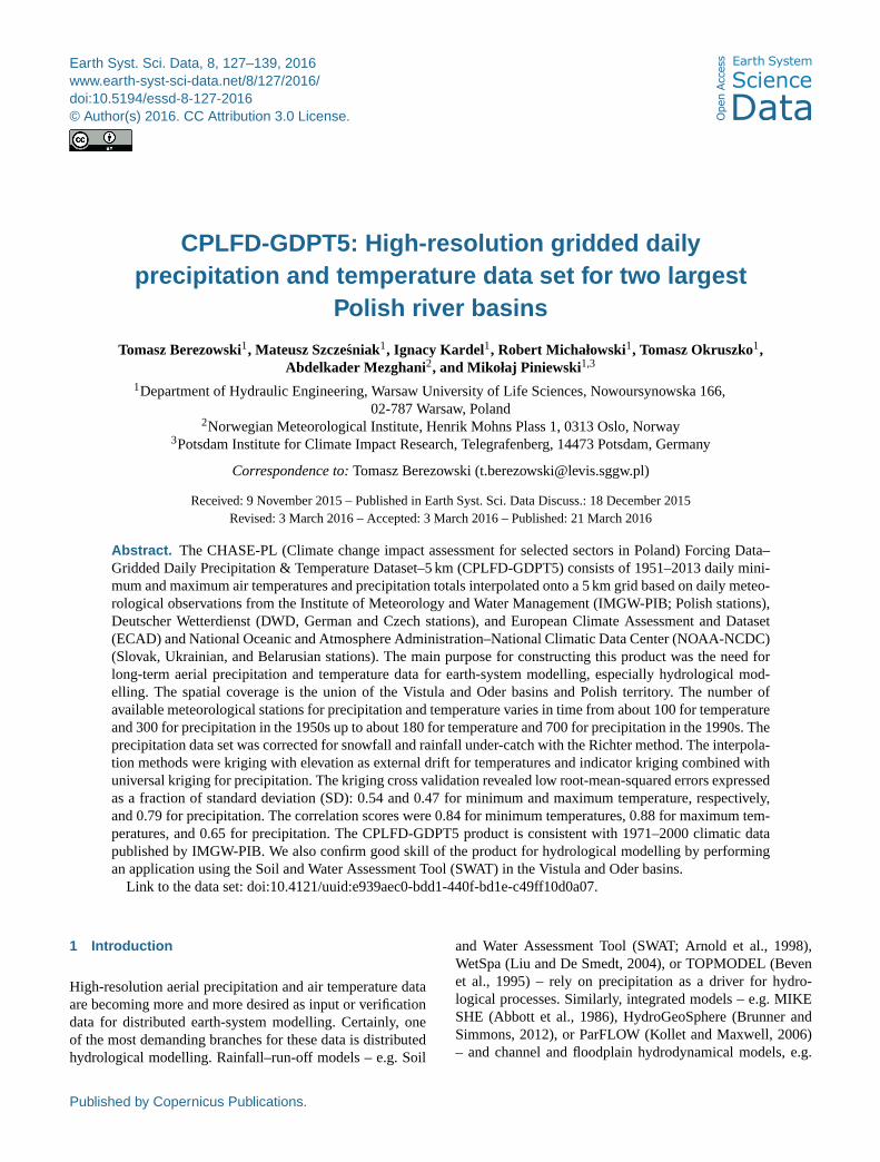
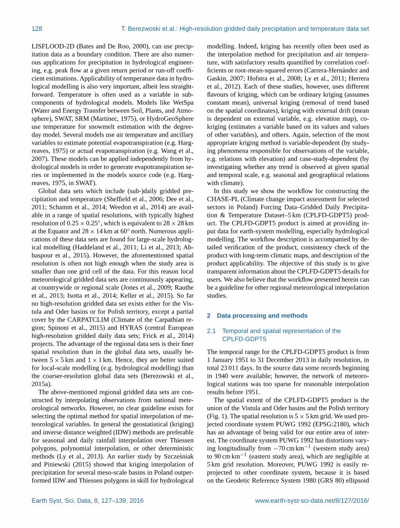
Temperature stationsPrecipitation stationsCPLFD-GDPT5 product extent
0 100 20050 km
Figure 4. Spatial distribution of meteorological stations for temper-
ature and precipitation used for interpolation of the CPLFD-GDPT5
product.
3. The corrected precipitation (mm) is calculated based on
Richter (1995) formulae as p = bpε , where p is the
measured precipitation total (mm), b is the coefficient
(–) for the influence of wind exposition of the measure-
ments site, and ε is a seasonally varying empiric coef-
ficient (–) for the precipitation type (snow, mixed snow
and rain, or rain). The range of b and ε values used in
this paper is available in Richter (1995). The values of b
were set as for “medium shielding” for all stations apart
from those in the mountains or close to the coast, where
b were set as for “low shielding” (Fig. 5). The rationale
behind assigning different values of b for different loca-
tion lies in the fact that wind speed is generally higher
in mountains and at the seaside than in the lowlands.
2.5 Interpolation
Our meteorological observations with spatial coordinates af-
ter pre-processing steps described above (Sects. 2.2–2.4)
were interpolated with two different kriging methods. Mini-
mum and maximum temperatures were interpolated with the
kriging with external drift, and precipitation with universal
kriging. The exponential variogram model has been used in
each case, with the variogram parameters estimated automat-
ically for each daily kriging with the weighted least-squares
fit (Pebesma, 2014). The block kriging approach was used
with the block size equal to the output square grid size, i.e.
5 km. Computations were conducted in the R software (R
Core Team, 2015) with the “gstat” package (Pebesma, 2004).
Earth Syst. Sci. Data, 8, 127–139, 2016 www.earth-syst-sci-data.net/8/127/2016/
T. Berezwoski et al.: High-resolution gridded daily precipitation and temperature data set 131
PL
CZUA
BY
DE
SK
LTRU
Parameter b for precipitation stationsLow shieldingM edium shieldingNational borders
0 100 20050 km
Figure 5. The Richter (1995) parameter b value groups for different
precipitation stations.
2.5.1 Temperature kriging
Both minimum and maximum temperatures were interpo-
lated in the same way. Kriging with external drift was used
in order to account for the temperature variability with ele-
vation. This approach was used in other similar studies (e.g.
Hattermann et al., 2005; Haylock et al., 2008). The exter-
nal drift variable was elevation (m) obtained from the Shuttle
Radar Topography Mission (SRTM) digital elevation model
aggregated to a 5 km grid. In order to remove the no-data
values from the SRTM data, the elevation of seas and oceans
was relabelled to 0.0 m.
2.5.2 Precipitation kriging
Precipitation was interpolated using a two-step approach
combining the universal kriging of the precipitation data
(first step) with the indicator kriging of the precipitation oc-
currence data (second step). This approach was selected due
to giving good results with a similar problem (e.g. Herrera
et al., 2012). Universal kriging was chosen because the trend
was not removed from the precipitation data beforehand. In-
dicator kriging was applied on binary data in order to allow
reducing the smoothing effect of around 0-value zones. The
daily precipitation totals p in each station were reclassified
to binary according to{0 if p < 0.1mm
1 if p ≥ 0.1mm.
The 0.1 mm threshold value was used as it reflects the error
due to rain gauges which is measured by ISO standards. As a
result of the indicator kriging a raster of real values ranging
between 0 and 1 was obtained; these values represent prob-
abilities of a day being wet, i.e. precipitation being equal
to 0.1 mm or higher, or “wet-day probabilities”. This raster
was used to mask the very small precipitation totals obtained
from the universal kriging of precipitation data (first step).
The mask was applied if the indicator kriging interpolation
value was smaller than a threshold. Usually a value of 0.5 is
selected as the threshold because it represent the 50 % prob-
ability, but in our case better results were obtained with a
smaller threshold, equal to 0.1. In the final step any negative
precipitation values (if still present) were changed to 0.
2.5.3 Cross validation
For each daily interpolation a cross validation was performed
for all stations; i.e. each station was removed from the sample
one at a time, and the remaining stations were used to predict
the value of the missing station.
The cross validation was conducted on both a temporal and
spatial scale. On the temporal scale the errors were calculated
for each day from all stations having data on this day. Due to
a high number of records in the temporal scale, we present
the results in the form of a descriptive statistics table. On the
spatial scale the errors are calculated for each station from all
of a station’s available daily values. The number of records
on the spatial scale calculation is equal to the number of me-
teorological stations used; hence, we present the result in the
form of maps.
The interpolation errors were quantified using two func-
tions: (1) the Pearson’s correlation coefficient (ρ (–)) and
(2) the root-mean-squared error normalized to the standard
deviation of the observed data (–):
RMSEsd=
√1N
∑Ni=1
(Yi − Yi
)2
σY,
where Y and Y are respectively the observed and interpolated
values of a given variable (precipitation or temperature), N
is the number of observations (number of stations in the spa-
tial approach or number of days in the temporal approach),
and σY is the standard deviation of observations. The ρ val-
ues show the collinearity of the observed and interpolated
data, and the RMSEsd values show the interpolation error as
a fraction of the observation standard deviation. Note that ρ
and RMSEsd can not be calculated for days with no observed
precipitation (i.e. precipitation at all stations is 0.0 mm) be-
cause the standard deviation is 0.0 mm (N = 154). Because
of that, these days were excluded from the cross-validation
analysis.
www.earth-syst-sci-data.net/8/127/2016/ Earth Syst. Sci. Data, 8, 127–139, 2016
132 T. Berezwoski et al.: High-resolution gridded daily precipitation and temperature data set
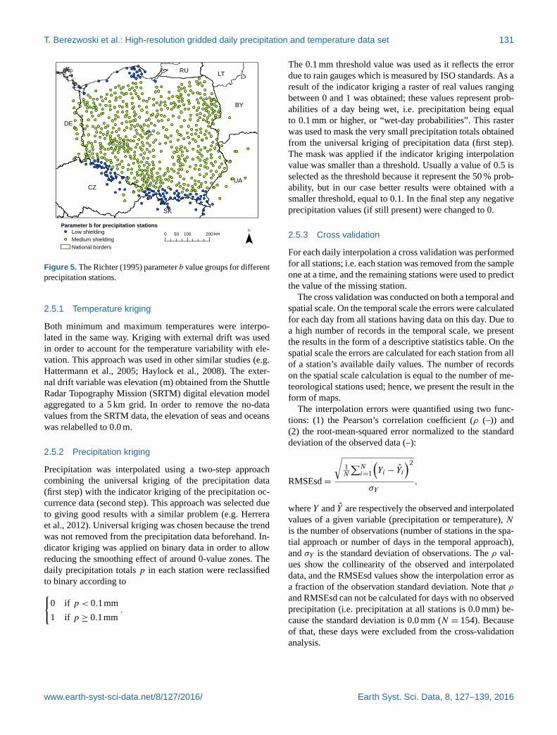
Table 1. Descriptive statistics for the kriging cross-validation results for precipitation, minimum temperature, and maximum temperature.
“ρ < 0” denotes percentage of ρ values lower than 0. “RMSEsd> 1” denotes percentage of RMSEsd values higher than 1.
Precipitation Minimum temperature Maximum temperature
ρ RMSEsd ρ RMSEsd ρ RMSEsd
Minimum −0.08 0.22 −2.00× 10⁻³ 0.14 −0.10 0.17
1st quartile 0.47 0.64 0.77 0.46 0.85 0.41
Median 0.65 0.79 0.84 0.54 0.88 0.47
3rd quartile 0.78 0.93 0.89 0.63 0.91 0.53
Maximum 0.98 1.37 0.99 1.03 0.99 1.13
ρ < 0 1.6 % – 4× 10⁻³ % – 4× 10⁻³ % –
RMSEsd> 1 – 14.2 % – 3× 10⁻⁴ % – 4× 10⁻⁴ %
PL
UACZ
BY
DE
SK
LTRU
0 100 20050
Correlation for precipitation stations0.00– 0.20 0.21– 0.40 0.41– 0.60 0.61– 0.80 0.81– 1.00
PL
UACZ
BY
DE
SK
LTRU
RMSEsd for precipitation stations0.29– 0.35 0.36– 0.70 0.71– 1.05 1.06– 1.40 1.41– 1.75
km
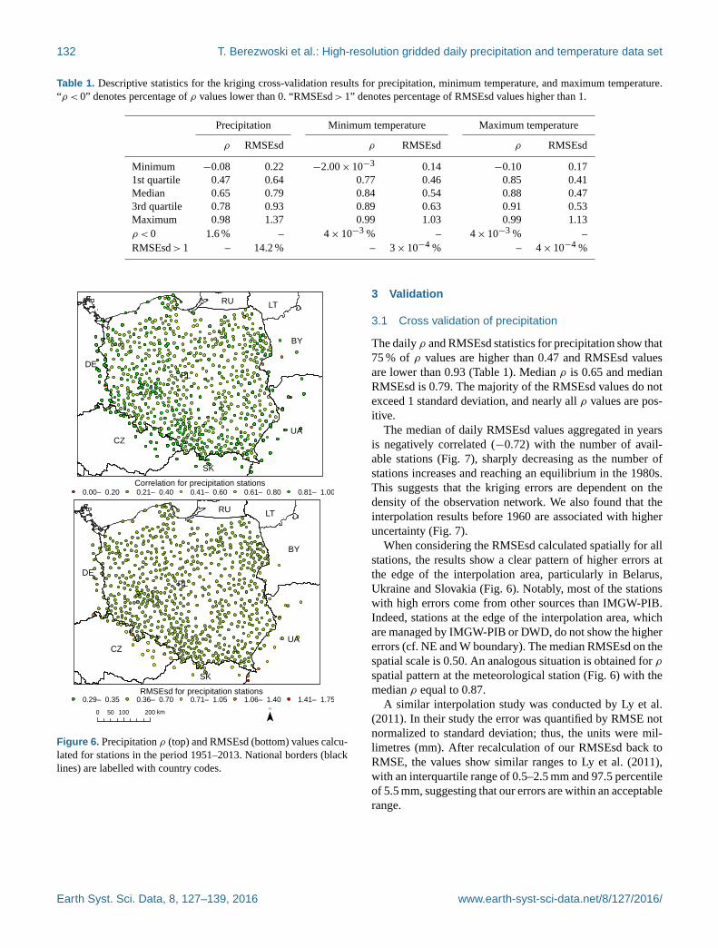
Figure 6. Precipitation ρ (top) and RMSEsd (bottom) values calcu-
lated for stations in the period 1951–2013. National borders (black
lines) are labelled with country codes.
3 Validation
3.1 Cross validation of precipitation
The daily ρ and RMSEsd statistics for precipitation show that
75 % of ρ values are higher than 0.47 and RMSEsd values
are lower than 0.93 (Table 1). Median ρ is 0.65 and median
RMSEsd is 0.79. The majority of the RMSEsd values do not
exceed 1 standard deviation, and nearly all ρ values are pos-
itive.
The median of daily RMSEsd values aggregated in years
is negatively correlated (−0.72) with the number of avail-
able stations (Fig. 7), sharply decreasing as the number of
stations increases and reaching an equilibrium in the 1980s.
This suggests that the kriging errors are dependent on the
density of the observation network. We also found that the
interpolation results before 1960 are associated with higher
uncertainty (Fig. 7).
When considering the RMSEsd calculated spatially for all
stations, the results show a clear pattern of higher errors at
the edge of the interpolation area, particularly in Belarus,
Ukraine and Slovakia (Fig. 6). Notably, most of the stations
with high errors come from other sources than IMGW-PIB.
Indeed, stations at the edge of the interpolation area, which
are managed by IMGW-PIB or DWD, do not show the higher
errors (cf. NE and W boundary). The median RMSEsd on the
spatial scale is 0.50. An analogous situation is obtained for ρ
spatial pattern at the meteorological station (Fig. 6) with the
median ρ equal to 0.87.
A similar interpolation study was conducted by Ly et al.
(2011). In their study the error was quantified by RMSE not
normalized to standard deviation; thus, the units were mil-
limetres (mm). After recalculation of our RMSEsd back to
RMSE, the values show similar ranges to Ly et al. (2011),
with an interquartile range of 0.5–2.5 mm and 97.5 percentile
of 5.5 mm, suggesting that our errors are within an acceptable
range.
Earth Syst. Sci. Data, 8, 127–139, 2016 www.earth-syst-sci-data.net/8/127/2016/

T. Berezwoski et al.: High-resolution gridded daily precipitation and temperature data set 133
Year
1960 1980 2000
0.70
0.75
0.80
0.85
0.90
300
400
500
600
700
Num
ber
of s
tatio
ns p
er y
ear
RM
SE
sd [−
]
Figure 7. Annual RMSEsd median (blue) and number of available
stations per year (pink) for precipitation in the period 1951–2013.
The daily results, also summarized in Table 1, were used for calcu-
lating the annual medians.
3.2 Cross validation of temperature
The statistics of daily RMSEsd show the median equal to
0.54 for the minimum temperature and 0.47 for maximum
temperature (Table 1). Nearly all the RMSEsd values in both
cases do not exceed 1 standard deviation, and the ρ values are
positive. The daily ρ statistics for minimum and maximum
temperature show that 75 % of ρ values are above 0.77 for
minimum temperature and above 0.86 for maximum temper-
ature. The median of ρ is 0.84 for the minimum temperature
and 0.88 for the maximum temperature.
The median of daily RMSEsd values for minimum tem-
perature aggregated in years is not correlated (0.00) with the
number of available stations (Fig. 10). The RMSEsd reached
a minimum in the 1970s. Since then, however, it has been
gradually increasing (at a small rate), which does not seem
to be related to changes in the number of available stations.
The situation is only slightly different for the maximum tem-
peratures (Fig. 11), for which correlation with the number of
stations is weak (0.22). Although the lowest RMSEsd can be
observed for the 1960s, since then a gradual increase (again,
at a small rate) can be observed. It should also be noted that
the range of RMSEsd is not very wide, in general (0.48–0.6
for the minimum temperature and 0.42–0.5, neglecting one
outlier, for the maximum temperature). Overall, it seems that
our kriging errors for temperature are not dependent on the
density of the observation network. However, as in the case
of precipitation interpolation the results before 1960 are as-
sociated with higher uncertainties.
When the RMSEsd results calculated spatially for all sta-
tions are analysed, the minimum temperature shows a rather
uniformly distributed values with a few outliers located at the
boundary of the interpolation area, mostly in the mountains
(southern border, Fig. 8). An analogous situation is observed
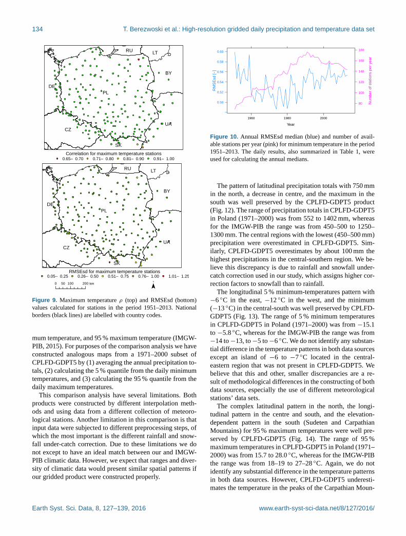
for maximum temperatures (Fig. 9). The median RMSEsd on
the spatial scale is equal to 0.17 for minimum temperature
and 0.10 for maximum temperature. An analogous situation
is observed for ρ spatial pattern for the meteorological sta-
PL
UACZ
BY
DE
SK
LTRU
0 100 20050
Correlation for minimum temperature stations0.46– 0.60 0.61– 0.80 0.81– 1.00
PL
UACZ
BY
DE
SK
LTRU
RMSEsd for minimum temperature stations0.06– 0.20 0.21– 0.40 0.41– 0.60 0.61– 0.80 0.81– 1.00
km
Figure 8. Minimum temperature ρ (top) and RMSEsd (bottom) val-
ues calculated for stations in the period 1951–2013. National bor-
ders (black lines) are labelled with country codes.
tion with the median ρ equal to 0.99 both for minimum and
maximum temperature.
A similar interpolation exercise was conducted by Carrera-
Hernández and Gaskin (2007). In their study the error was
quantified by ρ2. The ranges of ρ2 obtained in their study
were 0.73–0.88 for the maximum temperature and 0.68–0.96
for the minimum temperature. These results are very similar
to ours (after recalculating ρ to ρ2), suggesting good quality
of the gridded temperature data set.
4 Consistency with climatic data
The precipitation and minimum- and maximum-temperature
gridded products were analysed for consistency with long-
term climatic data. Since the majority of our product spatial
coverage is in Poland, we have used long-term climatic maps
from the Polish meteorological service (IMGW-PIB) for
comparison. The IMGW-PIB maps were developed for the
period 1971–2000 and include precipitation totals, 5 % mini-
www.earth-syst-sci-data.net/8/127/2016/ Earth Syst. Sci. Data, 8, 127–139, 2016
134 T. Berezwoski et al.: High-resolution gridded daily precipitation and temperature data set
PL
UACZ
BY
DE
SK
LTRU
0 100 20050
Correlation for maximum temperature stations0.65– 0.70 0.71– 0.80 0.81– 0.90 0.91– 1.00
PL
UACZ
BY
DE
SK
LTRU
RMSEsd for maximum temperature stations0.05– 0.25 0.26– 0.50 0.51– 0.75 0.76– 1.00 1.01– 1.25
km
Figure 9. Maximum temperature ρ (top) and RMSEsd (bottom)
values calculated for stations in the period 1951–2013. National
borders (black lines) are labelled with country codes.
mum temperature, and 95 % maximum temperature (IMGW-
PIB, 2015). For purposes of the comparison analysis we have
constructed analogous maps from a 1971–2000 subset of
CPLFD-GDPT5 by (1) averaging the annual precipitation to-
tals, (2) calculating the 5 % quantile from the daily minimum
temperatures, and (3) calculating the 95 % quantile from the
daily maximum temperatures.
This comparison analysis have several limitations. Both
products were constructed by different interpolation meth-
ods and using data from a different collection of meteoro-
logical stations. Another limitation in this comparison is that
input data were subjected to different preprocessing steps, of
which the most important is the different rainfall and snow-
fall under-catch correction. Due to these limitations we do
not except to have an ideal match between our and IMGW-
PIB climatic data. However, we expect that ranges and diver-
sity of climatic data would present similar spatial patterns if
our gridded product were constructed properly.
Year
1960 1980 2000
0.50
0.52
0.54
0.56
0.58
0.60
80
100
120
140
160
180
Num
ber
of s
tatio
ns p
er y
ear
RM
SE
sd [−
]
Figure 10. Annual RMSEsd median (blue) and number of avail-
able stations per year (pink) for minimum temperature in the period
1951–2013. The daily results, also summarized in Table 1, were
used for calculating the annual medians.
The pattern of latitudinal precipitation totals with 750 mm
in the north, a decrease in centre, and the maximum in the
south was well preserved by the CPLFD-GDPT5 product
(Fig. 12). The range of precipitation totals in CPLFD-GDPT5
in Poland (1971–2000) was from 552 to 1402 mm, whereas
for the IMGW-PIB the range was from 450–500 to 1250–
1300 mm. The central regions with the lowest (450–500 mm)
precipitation were overestimated in CPLFD-GDPT5. Sim-
ilarly, CPLFD-GDPT5 overestimates by about 100 mm the
highest precipitations in the central-southern region. We be-
lieve this discrepancy is due to rainfall and snowfall under-
catch correction used in our study, which assigns higher cor-
rection factors to snowfall than to rainfall.
The longitudinal 5 % minimum-temperatures pattern with
−6 ◦C in the east, −12 ◦C in the west, and the minimum
(−13 ◦C) in the central-south was well preserved by CPLFD-
GDPT5 (Fig. 13). The range of 5 % minimum temperatures
in CPLFD-GDPT5 in Poland (1971–2000) was from −15.1
to −5.8 ◦C, whereas for the IMGW-PIB the range was from
−14 to−13, to−5 to−6 ◦C. We do not identify any substan-
tial difference in the temperature patterns in both data sources
except an island of −6 to −7 ◦C located in the central-
eastern region that was not present in CPLFD-GDPT5. We
believe that this and other, smaller discrepancies are a re-
sult of methodological differences in the constructing of both
data sources, especially the use of different meteorological
stations’ data sets.
The complex latitudinal pattern in the north, the longi-
tudinal pattern in the centre and south, and the elevation-
dependent pattern in the south (Sudeten and Carpathian
Mountains) for 95 % maximum temperatures were well pre-
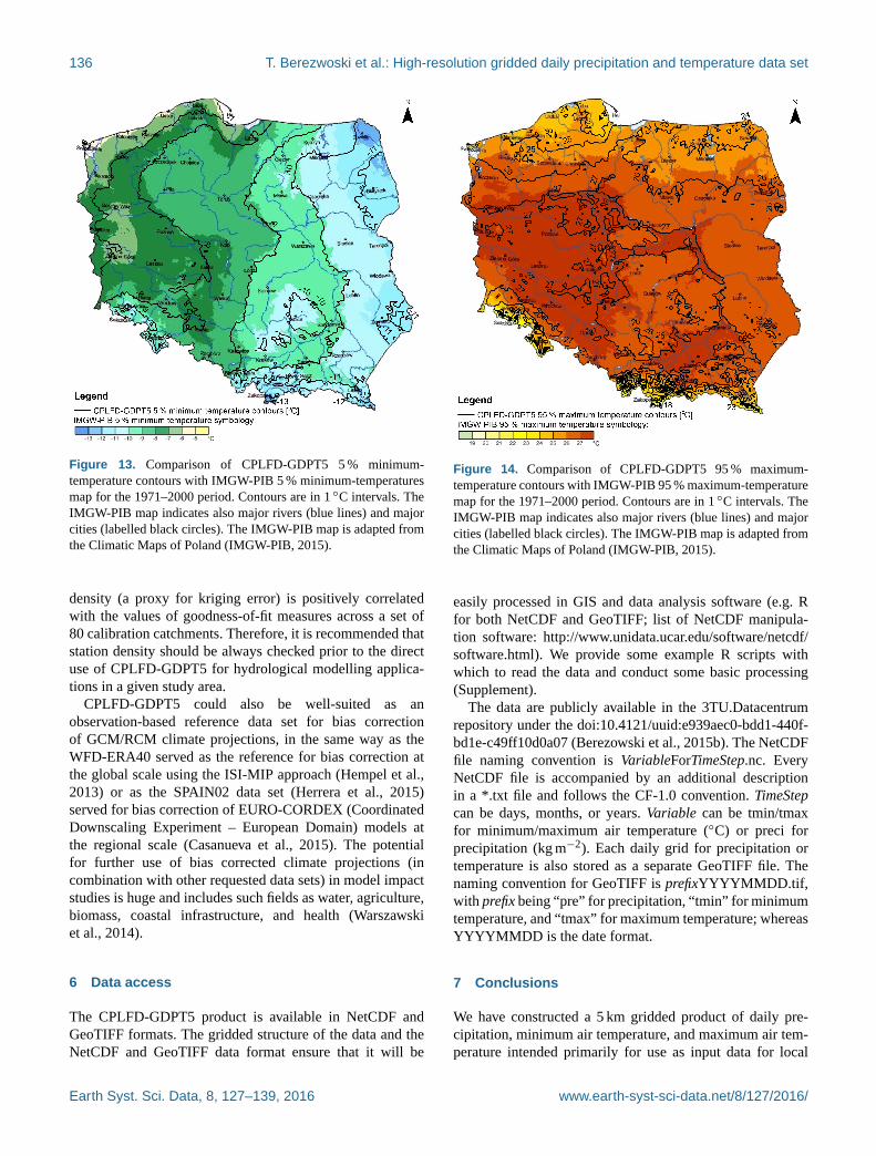
served by CPLFD-GDPT5 (Fig. 14). The range of 95 %
maximum temperatures in CPLFD-GDPT5 in Poland (1971–
2000) was from 15.7 to 28.0 ◦C, whereas for the IMGW-PIB
the range was from 18–19 to 27–28 ◦C. Again, we do not
identify any substantial difference in the temperature patterns
in both data sources. However, CPLFD-GDPT5 underesti-
mates the temperature in the peaks of the Carpathian Moun-
Earth Syst. Sci. Data, 8, 127–139, 2016 www.earth-syst-sci-data.net/8/127/2016/

T. Berezwoski et al.: High-resolution gridded daily precipitation and temperature data set 135
Year
1960 1980 2000
0.45
0.50
0.55
80
100
120
140
160
180
Num
ber
of s
tatio
ns p
er y
ear
RM
SE
sd [−
]
Figure 11. Annual RMSEsd median (blue) and number of avail-
able stations per year (pink) for maximum temperature in the period
1951–2013. The daily results, also summarized in Table 1, were
used for calculating the annual medians.
tains by about 2 ◦C. More clutter is also observed in our prod-
uct in the entire region, especially in the south (mountains).
We believe that these discrepancies are a result, as in the pre-
vious cases, of methodological differences in the construct-
ing of both data sources, especially the use of high-resolution
and detailed elevation data in our study, including differences
in the available stations used.
5 Applicability
This product was developed with the purpose of its further
(re)use for earth-system modelling, and in particular for hy-
drological modelling and climate impact studies. The spatial
resolution (5 km) of CPLFD-GDPT5 ensures that it will be
useful not only for regional studies, where generally lower-
resolution data would be appropriate, but also for modelling
on the local scale, where high spatial resolution is necessary
to capture the variability.
As an example application of CPLFD-GDPT5 for hy-
drological modelling, we have set up, calibrated, and val-
idated the SWAT model for the Vistula and Oder basins
(Piniewski et al., 2016). SWAT is a process-based, semi-
distributed, continuous-time hydrological model that simu-
lates the movement of water, sediment, and nutrients on a
catchment scale with a daily time step (Arnold et al., 1998).
Apart from the CPLFD-GDPT5 precipitation and tempera-
tures that are major input data, the SWAT set-up of the Vis-
tula and Oder basins uses various spatial input data such as
topography, hydrography, land cover, and soils, all with quite
complex parametrizations. Figure 15a shows spatial variabil-
ity of mean annual potential evapotranspiration (PET) cal-
culated in SWAT using the Hargreaves (1975) method, re-
lying on our minimum- and maximum-temperature data. In
the Hargreaves method PET is proportional to mean tem-
perature (approximated by the arithmetic mean of minimum
and maximum temperature) and the difference between max-
imum and minimum temperature (being a proxy of solar ra-
diation). As illustrated in many studies, the Hargreaves PET
Figure 12. Comparison of CPLFD-GDPT5 precipitation-totals
contours with IMGW-PIB precipitation-totals map for the 1971–
2000 period. Contours are in 50 mm intervals. The IMGW-PIB map
indicates also major rivers (blue lines) and major cities (labelled
black circles). The IMGW-PIB map is adapted from the Climatic
Maps of Poland (IMGW-PIB, 2015).
is highly correlated to other methods for PET estimations
(Lu et al., 2005) and to PET observations (Hargreaves and
Allen, 2003). Moreover, it was found particularly useful for
SWAT modelling by decreasing the observed PET estimation
error when compared to the Penman–Monteith PET estima-
tion (Earls and Dixon, 2008). Not surprisingly, the spatial
pattern in simulated PET largely follows the pattern of max-
imum temperature (Fig. 14).
PET constitutes an upper bound for actual evapotranspira-
tion, which is another variable simulated in SWAT, crucial for
the process of model calibration, typically performed using
measured discharge data. Figure 15b–c show two examples
of calibration plots illustrating simulated (95 % prediction
uncertainty band and one simulation with the highest value
of objective function) and measured daily stream flow from
the Vistula and Oder SWAT model developed in Piniewski
et al. (2016). The gauges were selected to demonstrate high
simulation skill of CPLFD-GDPT5 across a range of scales:
the Oder catchment upstream of Gozdowice is 110 000 km2,
while the Drweca River upstream of Rodzone is 1700 km2.
Both the positive visual inspection of the hydrograph and the
high values of objective functions (e.g. coefficient of deter-
mination equal to 0.81 and 0.71, respectively, and percent
bias of 1.4 and −5.8 %, respectively) confirm the useful-
ness and the quality of the developed interpolation product.
Piniewski et al. (2016) also showed that precipitation station
www.earth-syst-sci-data.net/8/127/2016/ Earth Syst. Sci. Data, 8, 127–139, 2016
136 T. Berezwoski et al.: High-resolution gridded daily precipitation and temperature data set
Figure 13. Comparison of CPLFD-GDPT5 5 % minimum-
temperature contours with IMGW-PIB 5 % minimum-temperatures
map for the 1971–2000 period. Contours are in 1 ◦C intervals. The
IMGW-PIB map indicates also major rivers (blue lines) and major
cities (labelled black circles). The IMGW-PIB map is adapted from
the Climatic Maps of Poland (IMGW-PIB, 2015).
density (a proxy for kriging error) is positively correlated
with the values of goodness-of-fit measures across a set of
80 calibration catchments. Therefore, it is recommended that
station density should be always checked prior to the direct
use of CPLFD-GDPT5 for hydrological modelling applica-
tions in a given study area.
CPLFD-GDPT5 could also be well-suited as an
observation-based reference data set for bias correction
of GCM/RCM climate projections, in the same way as the
WFD-ERA40 served as the reference for bias correction at
the global scale using the ISI-MIP approach (Hempel et al.,
2013) or as the SPAIN02 data set (Herrera et al., 2015)
served for bias correction of EURO-CORDEX (Coordinated
Downscaling Experiment – European Domain) models at
the regional scale (Casanueva et al., 2015). The potential
for further use of bias corrected climate projections (in
combination with other requested data sets) in model impact
studies is huge and includes such fields as water, agriculture,
biomass, coastal infrastructure, and health (Warszawski
et al., 2014).
6 Data access
The CPLFD-GDPT5 product is available in NetCDF and
GeoTIFF formats. The gridded structure of the data and the
NetCDF and GeoTIFF data format ensure that it will be
Figure 14. Comparison of CPLFD-GDPT5 95 % maximum-
temperature contours with IMGW-PIB 95 % maximum-temperature
map for the 1971–2000 period. Contours are in 1 ◦C intervals. The
IMGW-PIB map indicates also major rivers (blue lines) and major
cities (labelled black circles). The IMGW-PIB map is adapted from
the Climatic Maps of Poland (IMGW-PIB, 2015).
easily processed in GIS and data analysis software (e.g. R
for both NetCDF and GeoTIFF; list of NetCDF manipula-
tion software: http://www.unidata.ucar.edu/software/netcdf/
software.html). We provide some example R scripts with
which to read the data and conduct some basic processing
(Supplement).
The data are publicly available in the 3TU.Datacentrum
repository under the doi:10.4121/uuid:e939aec0-bdd1-440f-
bd1e-c49ff10d0a07 (Berezowski et al., 2015b). The NetCDF
file naming convention is VariableForTimeStep.nc. Every
NetCDF file is accompanied by an additional description
in a *.txt file and follows the CF-1.0 convention. TimeStep
can be days, months, or years. Variable can be tmin/tmax
for minimum/maximum air temperature (◦C) or preci for
precipitation (kg m−2). Each daily grid for precipitation or
temperature is also stored as a separate GeoTIFF file. The
naming convention for GeoTIFF is prefixYYYYMMDD.tif,
with prefix being “pre” for precipitation, “tmin” for minimum
temperature, and “tmax” for maximum temperature; whereas
YYYYMMDD is the date format.
7 Conclusions
We have constructed a 5 km gridded product of daily pre-
cipitation, minimum air temperature, and maximum air tem-
perature intended primarily for use as input data for local
Earth Syst. Sci. Data, 8, 127–139, 2016 www.earth-syst-sci-data.net/8/127/2016/

T. Berezwoski et al.: High-resolution gridded daily precipitation and temperature data set 137
Figure 15. Example application of CPLFD-GDPT5 in the hydro-
logical model SWAT of the Vistula and Oder basins. (a) Mean an-
nual potential evapotranspiration calculated using the Hargreaves
method based on daily minimum and maximum-temperature data.
(b) Simulated and observed daily stream flow on the Oder River
at Gozdowice gauging station. (c) Simulated and observed daily
stream flow on the Drweca River at Rodzone gauging station. Green
band denotes 95 % prediction uncertainty; blue and red lines denote
observed and simulated (best solution) flows, respectively.
and regional-scale modelling. The spatial extent of the prod-
uct is the union of the Oder and Vistula basins and the bor-
der of Poland. The input data for interpolation originates
from meteorological stations managed by many organiza-
tions. The stations are located in central Europe (western
Belarus, northern Czech Republic, eastern Germany, west-
ern Ukraine, the entirety of Poland, and northern Slovakia).
Various preprocessing steps were introduced in order to fil-
ter missing data and correct the precipitation for under-
catch. The quality of the product is assessed by a cross-
validation procedure conducted in parallel with the kriging
interpolation. The cross validation shows high correlations
and root-mean-squared errors lower than 1 standard devia-
tion of the observations in all three interpolated variables.
However, some particular stations located at the border of the
study area show slightly higher errors and lower correlations.
We also evaluated the consistency of our products with cli-
matic data provided by the Polish meteorological organiza-
tion (IMGW-PIB). The consistency check confirms the high
quality of the products, with only small differences result-
ing from different methodologies and number of selected sta-
tions across the region. Finally, we show an example appli-
cation of the gridded product for hydrological modelling in
SWAT. The results show very good discharge modelling ef-
ficiency in both a small and a large catchment, which shows
that the data set serves its purpose across a wide range of
scales. The high-resolution gridded data set will certainly
add value when used as a reference in bias-adjustment of re-
gional climate model results (e.g. EURO-CORDEX within
the CORDEX Initiative) by providing more reliable climate
projections for Poland.
The data set is provided in GeoTIFF and NetCDF format
in order to provide ease of access for most of the modelling
community. Nonetheless, we provide sample R scripts for
managing the data in the Supplement.
The data set and methods presented herein have several
aspects of further research. It would be interesting to com-
pare the data set with other data sets of lower resolution
(e.g. EOBS) in order to show its true added value for high-
resolution hydrological modelling. Moreover, the compar-
ison of the Hargreaves PET, estimated with the CPLFD-
GDPT5 temperatures, could be further investigated in the
scope of other PET estimation methods (e.g. Penman–
Monteith) and observations. Lastly, we believe that there is
still space to improve the interpolation methods by testing
other interpolation algorithms.
The CPLFD-GDPT5 product was constructed for the pe-
riod 1951–2013. New meteorological data and novel ap-
proaches to interpolation algorithms are continuously ap-
pearing. Hence, we are planning to update the product both
by extending the time span and by testing new interpolation
algorithms. The extension is planned on a 3-year basis.
The Supplement related to this article is available online
at doi:10.5194/essd-8-127-2016-supplement.
Acknowledgements. Support of the project CHASE-PL (Cli-
mate change impact assessment for selected sectors in Poland)
of the Polish–Norwegian Research Programme operated by the
National Centre for Research and Development (NCBiR) under
the Norwegian Financial Mechanism 2009–2014 in the frame
of project contract no. Pol-Nor/200799/90/2014 is gratefully
acknowledged. We also acknowledge the Institute of Meteorology
and Water Management–National Research Institute (IMGW-PIB),
www.earth-syst-sci-data.net/8/127/2016/ Earth Syst. Sci. Data, 8, 127–139, 2016

138 T. Berezwoski et al.: High-resolution gridded daily precipitation and temperature data set
Deutscher Wetterdienst (DWD), European Climate Assessment
and Dataset (ECAD), and National Oceanic and Atmosphere
Administration–National Climatic Data Center (NOAA-NCDC)
for providing meteorological data. The anonymous reviewer is
acknowledged for providing comments that considerably im-
proved the manuscript. Tobias Conradt from PIK, Potsdam, is
acknowledged for support in getting access to German climate
data. Mikołaj Piniewski is grateful for support from the Alexander
von Humboldt Foundation.
Edited by: G. König-Langlo
References
Abbaspour, K., Rouholahnejad, E., Vaghefi, S., Srinivasan, R.,
Yang, H., and Klove, B.: A continental-scale hydrology and wa-
ter quality model for Europe: Calibration and uncertainty of a
high-resolution large-scale SWAT model, J. Hydrol., 524, 733–
752, 2015.
Abbott, M., Bathurst, J., Cunge, J., O’Connell, P., and Rasmussen,
J.: An introduction to the European Hydrological System –
Systeme Hydrologique Europeen, “SHE”, 2: Structure of a
physically-based, distributed modelling system, J. Hydrol., 87,
61–77, 1986.
Arnold, J. G., Srinivasan, R., Muttiah, R. S., and Williams, J. R.:
Large Area Hydrologic Modeling And Assessment Part I: Model
Development, JAWRA J. Am. Water Resour. As., 34, 73–89,
1998.
Bates, P. and De Roo, A.: A simple raster-based model for flood
inundation simulation, J. Hydrol., 236, 54–77, 2000.
Berezowski, T., Chormanski, J., and Batelaan, O.: Skill of remote
sensing snow products for distributed runoff prediction, J. Hy-
drol., 524, 718–732, 2015a.
Berezowski, T., Szczesniak, M., Kardel, I., Michałowski, R., and
Piniewski, M.: CHASE-PL Forcing Data – Gridded Daily Pre-
cipitation & Temperature Dataset (CPLFD-GDPT5), Dataset on
3TU.Datacentrum, doi:10.4121/uuid:e939aec0-bdd1-440f-bd1e-
c49ff10d0a07, 2015b.
Beven, K., Lamb, R., Quinn, P., Romanowicz, R., and Freer, J.:
TOPMODEL, in: Computer Models of Watershed Hydrology,
edited by: Singh, V. P., Water Resources Publication, Colorado,
627–668, 1995.
Brunner, P. and Simmons, C. T.: HydroGeoSphere: A Fully Inte-
grated, Physically Based Hydrological Model, Ground Water, 50,
170–176, 2012.
Carrera-Hernández, J. and Gaskin, S.: Spatio temporal analysis of
daily precipitation and temperature in the Basin of Mexico, J.
Hydrol., 336, 231–249, 2007.
Casanueva, A., Kotlarski, S., Herrera, S., Fernández, J., Gutiérrez,
J., Boberg, F., Colette, A., Christensen, O., Goergen, K., Jacob,
D., Keuler, K., Nikulin, G., Teichmann, C., and Vautard, R.:
Daily precipitation statistics in a EURO-CORDEX RCM ensem-
ble: added value of raw and bias-corrected high-resolution simu-
lations, Clim. Dynam., 1–19, 2015.
Chomicz, K.: Factual Precipitation in Poland (1931–1960), Prz.
Geof., 21, 19–25, 1976 (in Polish).
Dee, D. P., Uppala, S. M., Simmons, A. J., Berrisford, P., Poli,
P., Kobayashi, S., Andrae, U., Balmaseda, M. A., Balsamo, G.,
Bauer, P., Bechtold, P., Beljaars, A. C. M., van de Berg, L., Bid-
lot, J., Bormann, N., Delsol, C., Dragani, R., Fuentes, M., Geer,
A. J., Haimberger, L., Healy, S. B., Hersbach, H., Holm, E. V.,
Isaksen, L., Kallberg, P., Kohler, M., Matricardi, M., McNally,
A. P., Monge-Sanz, B. M., Morcrette, J.-J., Park, B.-K., Peubey,
C., de Rosnay, P., Tavolato, C., Thepaut, J.-N., and Vitart, F.: The
ERA-Interim reanalysis: configuration and performance of the
data assimilation system, Q. J. Roy. Meteor. Soc., 137, 553–597,
2011.
Earls, J. and Dixon, B.: A comparison of SWAT model-predicted
potential evapotranspiration using real and modeled meteorolog-
ical data, Vadose Zone J., 7, 570–580, 2008.
Frick, C., Steiner, H., Mazurkiewicz, A., Riediger, U., Rauthe, M.,
Reich, T., and Gratzki, A.: Central European high-resolution
gridded daily data sets (HYRAS): Mean temperature and rela-
tive humidity, Meteorol. Z., 23, 15–32, 2014.
Goodison, B., Louie, P., and Yang, D.: WMO Solid Precipitation
Measurement Intercomparison, Final Report, 1998.
Haddeland, I., Clark, D. B., Franssen, W., Ludwig, F., Vos, F.,
Arnell, N. W., Bertrand, N., Best, M., Folwell, S., Gerten, D.,
Gomes, S., Gosling, S. N., Hagemann, S., Hanasaki, N., Harding,
R., Heinke, J., Kabat, P., Koirala, S., Oki, T., Polcher, J., Stacke,
T., Viterbo, P., Weedon, G. P., and Yeh, P.: Multimodel Estimate
of the Global Terrestrial Water Balance: Setup and First Results,
J. Hydrometeorol., 12, 869–884, 2011.
Hargreaves, G.: Moisture availability and crop prodution, T. ASAE,
18, 980–984, 1975.
Hargreaves, G. and Allen, R.: History and Evaluation of Hargreaves
Evapotranspiration Equation, J. Irrig. Drain. E-ASCE, 129, 53–
63, 2003.
Hattermann, F., Wattenbach, M., Krysanova, V., and Wechsung, F.:
Runoff simulations on the macroscale with the ecohydrological
model SWIM in the Elbe catchment–validation and uncertainty
analysis, Hydrol. Process., 19, 693–714, 2005.
Haylock, M. R., Hofstra, N., Klein Tank, A. M. G., Klok, E. J.,
Jones, P. D., and New, M.: A European daily high-resolution
gridded data set of surface temperature and precipitation for
1950–2006, J. Geophys. Res.-Atmos., 113, D20119, 2008.
Hempel, S., Frieler, K., Warszawski, L., Schewe, J., and Piontek, F.:
A trend-preserving bias correction – the ISI-MIP approach, Earth
Syst. Dynam., 4, 219–236, doi:10.5194/esd-4-219-2013, 2013.
Herrera, S., Gutiérrez, J. M., Ancell, R., Pons, M. R., Frias,
M. D., and Fernandez, J.: Development and analysis of a 50-year
high-resolution daily gridded precipitation dataset over Spain
(Spain02), Int. J. Climatol., 32, 74–85, 2012.
Herrera, S., Fernández, J., and Gutiérrez, J. M.: Update of the
Spain02 gridded observational dataset for EURO-CORDEX
evaluation: assessing the effect of the interpolation methodology,
Int. J. Climatol., 36, 900–908, doi:10.1002/joc.4391, 2015.
Hofstra, N., Haylock, M., New, M., Jones, P., and Frei, C.: Com-
parison of six methods for the interpolation of daily, Euro-
pean climate data, J. Geophys. Res.-Atmos., 113, D21110,
doi:10.1029/2008JD010100, 2008.
IMGW-PIB: Climatic maps for Poland, available at: http:
//www.imgw.pl/klimat/ (last access: 1 October 2015), ac-
cessed with the following options: Tab= “Wielolecie 1971–
200”, Sezon/Rok= “Rok”; (1) for precipitaion: Wybierz ele-
ment= “Suma opadu”; (2) for minimum temperature: Wybierz
Earth Syst. Sci. Data, 8, 127–139, 2016 www.earth-syst-sci-data.net/8/127/2016/

T. Berezwoski et al.: High-resolution gridded daily precipitation and temperature data set 139
element= “Temperatura minimalna”; (3) for maximum temper-
ature: Wybierz element= “Temperatura maksymalna”, 2015.
Isotta, F. A., Frei, C., Weilguni, V., Percec Tadic, M., Lassegues, P.,
Rudolf, B., Pavan, V., Cacciamani, C., Antolini, G., Ratto, S. M.,
Munari, M., Micheletti, S., Bonati, V., Lussana, C., Ronchi, C.,
Panettieri, E., Marigo, G., and Vertacnik, G.: The climate of daily
precipitation in the Alps: development and analysis of a high-
resolution grid dataset from pan-Alpine rain-gauge data, Int. J.
Climatol., 34, 1657–1675, 2014.
Jones, D. A., Wang, W., and Fawcett, R.: High-quality spatial
climate data-sets for Australia, Australian Meteorological and
Oceanographic Journal, 58, 233–248, 2009.
Keller, V. D. J., Tanguy, M., Prosdocimi, I., Terry, J. A., Hitt, O.,
Cole, S. J., Fry, M., Morris, D. G., and Dixon, H.: CEH-GEAR:
1 km resolution daily and monthly areal rainfall estimates for the
UK for hydrological and other applications, Earth Syst. Sci. Data,
7, 143–155, doi:10.5194/essd-7-143-2015, 2015.
Kollet, S. J. and Maxwell, R. M.: Integrated surface-groundwater
flow modeling: A free-surface overland flow boundary condition
in a parallel groundwater flow model, Adv. Water Resour., 29,
945–958, 2006.
Li, L., Ngongondo, C. S., Xu, C.-Y., and Gong, L.: Comparison of
the global TRMM and WFD precipitation datasets in driving a
large-scale hydrological model in Southern Africa, Hydrol. Res.,
10, 770–788, doi:10.2166/nh.2012.175, 2013.
Liu, Y. B. and De Smedt, F.: WetSpa Extension, A GIS-based
Hydrologic Model for Flood Prediction and Watershed Man-
agement, Department of Hydrology and Hydraulic Engineering,
Vrije Universiteit Brussel, 2004.
Lu, J., Sun, G., McNulty, S. G., and Amatya, D. M.: A comparison
of six potential evapotranspiration methods for regional use in
the southeastern United States1, J. Am. Water Resour. As., 41,
621–633, 2005.
Ly, S., Charles, C., and Degré, A.: Geostatistical interpolation of
daily rainfall at catchment scale: the use of several variogram
models in the Ourthe and Ambleve catchments, Belgium, Hy-
drol. Earth Syst. Sci., 15, 2259–2274, doi:10.5194/hess-15-2259-
2011, 2011.
Ly, S., Charles, C., and Degré, A.: Different methods for spatial in-
terpolation of rainfall data for operational hydrology and hydro-
logical modeling at watershed scale: A review, Biotechnologie,
Agronomie, Société et Environnement, 17, 392–406, 2013.
Martinec, J.: Snowmelt – Runoff Model For Stream Flow Forecasts,
Nordic Hydrol., 6, 145–154, 1975.
Menne, M. J., Durre, I., Vose, R. S., Gleason, B. E., and Houston,
T. G.: An overview of the global historical climatology network-
daily database, J. Atmos. Ocean. Techn., 29, 897–910, 2012.
Pebesma, E. J.: Multivariable geostatistics in S: the gstat package,
Comput. Geosci., 30, 683–691, 2004.
Pebesma, E. J.: gstat user’s manual, Dept. of Physical Geogra-
phy, Utrecht University, P.O. Box 80.115, 3508 TC, Utrecht, the
Netherlands, gstat 2.5.1 Edn., available at: http://www.gstat.org/
gstat.pdf (last access: 16 December 2015), 2014.
Piniewski, M., Szczessniak, M., Kardel, I., Berezowski, T.,
Okruszko, T., Srinivasan, R., Schuler, D. V., and Kundzewicz,
Z.: Modelling water balance and streamflow at high resolution in
the Vistula and Oder basins, Hydrolog Sci. J., submitted, 2016.
Project team ECAD: European Climate Assessment & Dataset
(ECA&D), Algorithm Theoretical Basis Document (ATBD),
Royal Netherlands Meteorological Institute KNMI, the Nether-
lands, 2013.
Rauthe, M., Steiner, H., Riediger, U., Mazurkiewicz, A., and
Gratzki, A.: A Central European precipitation climatology – Part
I: Generation and validation of a high-resolution gridded daily
data set (HYRAS), Meteorol. Z., 22, 235–256, 2013.
R Core Team: R: A Language and Environment for Statistical Com-
puting, R Foundation for Statistical Computing, Vienna, Austria,
available at: https://www.R-project.org/ (last access: 16 Decem-
ber 2015), 2015.
Richter, D.: Ergebnisse methodischer Untersuchungen zur Ko-
rrektur des systematischen Messfehlers des Hellmannnieder-
schlagsmessers, Vol. 194, Berichte des Deutschen Wetterdien-
stes, 1995.
Schamm, K., Ziese, M., Becker, A., Finger, P., Meyer-Christoffer,
A., Schneider, U., Schröder, M., and Stender, P.: Global grid-
ded precipitation over land: a description of the new GPCC
First Guess Daily product, Earth Syst. Sci. Data, 6, 49–60,
doi:10.5194/essd-6-49-2014, 2014.
Sheffield, J., Goteti, G., and Wood, E. F.: Development of a 50-Year
High-Resolution Global Dataset of Meteorological Forcings for
Land Surface Modeling, J. Climate, 19, 3088–3111, 2006.
Spinoni, J., Szalai, S., Szentimrey, T., Lakatos, M., Bihari, Z., Nagy,
A., Nemeth, A., Kovacs, T., Mihic, D., Dacic, M., Petrovic, P.,
Krzic, A., Hiebl, J., Auer, I., Milkovic, J., Stepanek, P., Zahrad-
nicek, P., Kilar, P., Limanowka, D., Pyrc, R., Cheval, S., Birsan,
M.-V., Dumitrescu, A., Deak, G., Matei, M., Antolovic, I., Nejed-
lik, P., Stastny, P., Kajaba, P., Bochnicek, O., Galo, D., Mikulova,
K., Nabyvanets, Y., Skrynyk, O., Krakovska, S., Gnatiuk, N., To-
lasz, R., Antofie, T., and Vogt, J.: Climate of the Carpathian Re-
gion in the period 1961–2010: climatologies and trends of 10
variables, Int. J. Climatol., 35, 1322–1341, 2015.
Szczesniak, M. and Piniewski, M.: Improvement of Hydrologi-
cal Simulations by Applying Daily Precipitation Interpolation
Schemes in Meso-Scale Catchments, Water, 7, 747–779, 2015.
Wang, K., Wang, P., Li, Z., Cribb, M., and Sparrow, M.: A simple
method to estimate actual evapotranspiration from a combination
of net radiation, vegetation index, and temperature, J. Geophys.
Res.-Atmos., 112, D15107, doi:10.1029/2006JD008351, 2007.
Warszawski, L., Frieler, K., Huber, V., Piontek, F., Serdeczny, O.,
and Schewe, J.: The Inter-Sectoral Impact Model Intercompar-
ison Project (ISI–MIP): Project framework, P. Natl. Acad. Sci.,
111, 3228–3232, 2014.
Weedon, G. P., Balsamo, G., Bellouin, N., Gomes, S., Best, M. J.,
and Viterbo, P.: The WFDEI meteorological forcing data set:
WATCH Forcing Data methodology applied to ERA-Interim re-
analysis data, Water Resour. Res., 50, 7505–7514, 2014.
WMO: National Meteorological or Hydrometeorological Services
of Members, available at: https://www.wmo.int/pages/members/
members_en.html (last access: 16 December 2015), 2015.
www.earth-syst-sci-data.net/8/127/2016/ Earth Syst. Sci. Data, 8, 127–139, 2016