envisioning urban growth patterns that support...
TRANSCRIPT
1
ENVISIONING URBAN GROWTH PATTERNS THAT SUPPORT LONG-RANGE PLANNING GOALS – A COMPARATIVE ANALYSIS OF TWO METHODS OF
FORECASTING FUTURE LAND USE CHANGE
By
ELIZABETH A. THOMPSON
A THESIS PRESENTED TO THE GRADUATE SCHOOL OF THE UNIVERSITY OF FLORIDA IN PARTIAL FULFILLMENT
OF THE REQUIREMENTS FOR THE DEGREE OF MASTER OF ARTS IN URBAN AND REGIONAL PLANNING
UNIVERSITY OF FLORIDA
2010

2
© 2010 Elizabeth A. Thompson

3
To Amelie Helen Thompson, my beloved daughter and guiding light

4
ACKNOWLEDGMENTS
My sincere thanks and gratitude are bestowed upon my generous and supportive
committee members Dr. Paul Zwick and Dr. Ruth Steiner. As chair of my committee,
Dr. Zwick has been instrumental in nurturing and guiding my research journey in a way
that continually challenges me to think “outside of the box” so that I might learn to see
more than what is first apparent. If not for Dr. Zwick‟s support and guidance I could not
have reached this important personal goal, and so to him I am truly indebted. As my
committee co-chair Dr. Steiner has been equally important by helping me navigate the
often murky waters of understanding the relationship between land use and
transportation. Without her vast knowledge, advice and guidance I would have certainly
stumbled along the way far more than I did, so to her I am also very thankful. Thanks
also to Dr. Zhong-Ren Peng for introducing me to the world of transportation demand
modeling and for gladly giving assistance whenever it was needed.
To my fellow LUCIS-ists, Iris Patten, Emily Stallings, Naser Arafat, Christen Hutton
and Yuyang Zou, I owe a large measure of thanks, not only for their technical support
and advice at all hours of the night and day but also for their sincere friendship which
has meant a great deal to me.
The love and support of my family made this whole journey possible, without their
encouragement I surely would not have had the strength to reach this goal. I shall
always be indebted to my parents Marshall and JoAn Wrightstone, and my parents-in-
law, Keith and Marilyn Thompson who have helped me in more ways than I can ever
mention here.
And above all others I owe the most thanks to my adoring husband Kevin and
precious daughter Amelie who have endured my lengthy distractedness, frequent

5
frustrations and occasional bad temper, but love me nonetheless. I could not have
done this without you both, nor would I ever want to.

6
TABLE OF CONTENTS page
ACKNOWLEDGMENTS .................................................................................................. 4
LIST OF TABLES .......................................................................................................... 10
LIST OF FIGURES ........................................................................................................ 12
LIST OF ABBREVIATIONS ........................................................................................... 13
ABSTRACT ................................................................................................................... 15
CHAPTER
1 INTRODUCTION .................................................................................................... 17
The Challenge of Forecasting the Future................................................................ 17
Research Argument and Study Objective ............................................................... 18 Study Outline .......................................................................................................... 19
2 LITERATURE REVIEW .......................................................................................... 21
Introduction ............................................................................................................. 21 The Land Use - Transportation Relationship .......................................................... 23
The Spatial Evolution of Urban America ........................................................... 24 Walking-Horsecar era (1800 – 1890) ......................................................... 24
Electric streetcar era (1890 – 1920) ........................................................... 24 Recreational automobile era (1920 – 1945) ............................................... 25 Freeway era (1945 – present) .................................................................... 26
Mobility and Accessibility – Key Concepts........................................................ 27 Trends in Planning Approach and Research .................................................... 29
Meta-Analysis of Selected Literature Reviews ................................................. 34 Badoe and Miller (2000) ............................................................................. 36
Ewing and Cervero (2001) ......................................................................... 37 Handy (2005) ............................................................................................. 41 Transportation Research Board (2009) ...................................................... 43
Summary .......................................................................................................... 45 Transportation and Land Use Modeling .................................................................. 46
Transportation Modeling – The Four Step Model ............................................. 47 Overview .................................................................................................... 47 Sub-models ................................................................................................ 48
Land Use Modeling .......................................................................................... 53 Model types and operational characteristics .............................................. 53
Meta-analysis of selected literature reviews............................................... 55
Scenario Planning ................................................................................................... 59 History and Planning Applications .................................................................... 61

7
Strengths and Limitations ................................................................................. 63 Land Use Suitability Analysis .................................................................................. 66
Overview .......................................................................................................... 66
Land Use Conflict Identification Strategy (LUCIS) ............................................ 69 Summary ................................................................................................................ 74
3 STUDY AREA AND TIME FRAME ......................................................................... 77
Study Area Selection .............................................................................................. 77 Study Time Frame .................................................................................................. 86
4 METHODOLOGY ................................................................................................... 88
Methodology Overview ........................................................................................... 88
Step One ................................................................................................................. 90 Florida Land Use Allocation Method Scenario Data ......................................... 90 Land Use Conflict Identification Strategy Planning Land Use Scenarios
Data .............................................................................................................. 91
Step Two ................................................................................................................. 92 Transportation Analysis Zone Data – Overview ............................................... 92
FLUAM – the Florida Land Use Allocation Method ........................................... 93 Development of control totals ..................................................................... 93 Determination of developable lands ........................................................... 94
Input of approved developments, manual adjustments and overrides ....... 94 Allocation of growth to TAZs ...................................................................... 96
LUCIS-plus – The LUCIS Planning Land Use Scenarios Method .................... 97 Creation of combine raster to identify areas suitable for growth .............. 100
Establishment of existing gross densities ................................................ 110 Establishment of control totals for growth ................................................ 114 Allocation of existing population and employment using gross densities . 114
Establishment of guidelines for distribution of growth .............................. 115 Allocation of growth to suitable areas based on established guidelines ... 120
Step Three ............................................................................................................ 126 FLUAM Scenario – TAZ Data and Transit System ......................................... 127
LUCIS-Plus Scenarios – TAZ Data and Transit System ................................. 128 Central Florida Regional Planning Model – Model Run for Each Scenario .... 129
5 FINDINGS ............................................................................................................. 132
Compact Development ......................................................................................... 132 Energy Conservation ............................................................................................ 135
Single-Occupant Vehicle and Transit Trips ........................................................... 139 Summary .............................................................................................................. 140
6 DISCUSSION ....................................................................................................... 142
Discussion of Findings and Methods .................................................................... 142 Compact Development ................................................................................... 142
8
Increased Transit Ridership ............................................................................ 144 Decreased Dependency on SOV ................................................................... 146 Energy Conservation – Reduction in VMT...................................................... 148
Regional Accessibility and the Challenges of DRIs ........................................ 150 Proximity to Transit and Employment Densities ............................................. 151 Criticisms of the FSM and the CFRPM ........................................................... 151 Complex Land Use Models vs. Deterministic Approaches to Forecasting
Land Use Change ....................................................................................... 152
Study Limitations ............................................................................................ 153
7 CONCLUSION ...................................................................................................... 155
APPENDIX
A LAND USE MODELS REVIEWED BY AUTHOR AND MODEL TYPE ................. 161
B STRENGTHS AND LIMITATIONS OF LAND USE MODEL TYPES BY AUTHOR ............................................................................................................... 162
C DATA DICTIONARY FOR LUCIS-PLUS SCENARIOS ......................................... 164
D ZDATA1 AND ZDATA2 DESCRIPTIONS ............................................................. 165
E ALLOCATION BUFFERS 1 AND 2 ....................................................................... 166
F ALLOCATION BUFFER 3 ..................................................................................... 167
G ALLOCATION BUFFER 4 ..................................................................................... 168
H ALLOCATION BUFFER 5 ..................................................................................... 169
I AGGREGATION OF FDOR LAND USE CODES IN THE PARCEL DATA TO TAZ LAND USE CODES ...................................................................................... 170
J AGGREGATION OF ECFRPC EMPLOYMENT CATEGORIES TO TAZ LAND USE CODES ......................................................................................................... 171
K LAKE COUNTY 2009 – 2020 TRANSIT DEVELOPMENT PLAN – MAP AND DESCRIPTION OF MODES AND ROUTES ......................................................... 172
L TOD DESIGN STANDARDS USED AS STUDY GUIDELINES ............................ 173
M GENERAL SELECTION CRITERIA FOR ALLOCATION INTO BUFFERS 1 TO 5 FOR LOW AND HIGH LUCIS-PLUS SCENARIOS ........................................... 174
N STUDY AREA ROADS USED IN CFRPM BY AREA TYPE ................................. 175
O LUCIS-PLUS LOW SCENARIO POPULATION DENSITY ................................... 176

9
P LUCIS-PLUS HIGH SCENARIO POPULATION DENSITY ................................... 177
Q LUCIS-PLUS LOW SCENARIO EMPLOYMENT DENSITY ................................. 178
R LUCIS-PLUS HIGH SCENARIO EMPLOYMENT DENSITY ................................. 179
LIST OF REFERENCES ............................................................................................. 180
BIOGRAPHICAL SKETCH .......................................................................................... 186

10
LIST OF TABLES
Table page 2-1 Number of journal articles and book chapters resulting from literature search of
ScienceDirect database ...................................................................................... 30
2-2 Selected federal policies related to urban transportation planning ......................... 32
2-3 Meta-analysis of selected literature reviews – summary of findings ....................... 45
2-4 Selected literature reviews for meta-analysis of land use models .......................... 55
2-5 The six step LUCIS process. .................................................................................. 70
2-6 Example of a subset of goals, objectives and sub-objectives for the agriculture category .............................................................................................................. 71
3-1 Florida‟s population growth rates by region – percentage change per decade, 1900 to 2000....................................................................................................... 77
3-2 Florida‟s projected population increase (per thousand people) by region, 2010 to 2035 ............................................................................................................... 79
3-3 Florida‟s central region, gross population densities and increases from 2010 to 2035. .................................................................................................................. 81
3-4 Residence and work counties for workers in Lake, Osceola and Orange Counties for 1990 and 2000 ............................................................................... 82
3-5 Median values of owner-occupied houses in 2000 and 2008 ................................. 83
4-1 Total acreage by TAZ land use categories. .......................................................... 111
4-2 Census Bureau estimates for 2007 for Lake County population by residential TAZ land use categories ................................................................................... 111
4-3 TAZ estimates for 2007 for Lake County population by residential TAZ land use categories ......................................................................................................... 112
4-4 Existing gross residential densities for study area ............................................... 112
4-5 ECFRPC estimates for 2007 for Lake County employment by TAZ land use categories ......................................................................................................... 113
4-6 TAZ estimates for 2007 for Lake County employment by TAZ land use categories ......................................................................................................... 113
4-7 Existing gross employment densities for study area ............................................ 114

11
4-8 Population and employment control totals ........................................................... 114
4-9 NEW_LU codes.................................................................................................... 115
4-10 Transit systems A and B – routes, modes, and headways ................................. 127
5-1 Population and employment distribution – FLUAM and LUCIS-plus scenarios compared to 2007 TAZ data ............................................................................. 134
5-2 Average TAZ population and employment densities by buffers ........................... 135
5-3 Daily volume of vehicle-miles traveled in Lake County – comparison of transit systems by land use scenario........................................................................... 136
5-4 Daily volume of vehicle-miles traveled in Lake County – comparison of all scenarios for transit system B ........................................................................... 136
5-5 Vehicle-miles traveled in Lake County by transit system B – comparison of LUCIS-plus low and FLUAM scenarios by area type ........................................ 137
5-6 Vehicle-miles traveled in Lake County by transit System B – comparison of the FLUAM and LUCIS-plus low scenarios by area type ........................................ 137
5-7 Vehicle-miles traveled in Lake County by transit System B – comparison of the FLUAM and LUCIS-plus high scenarios by area type ...................................... 138
5-8 Vehicle-miles traveled in Lake County by transit System B – comparison of LUCIS-plus low and LUCIS-plus high scenarios by area type .......................... 138
5-9 Daily volume of home-based work and non-home-based work trips in Lake County by mode – all scenarios ........................................................................ 140

12
LIST OF FIGURES
Figure page 2-1 Example of mutually supportive land use and transportation planning goals. ...... 22
2-2 Methods of interpreting planning goals and their relationship. ............................... 23
2-3 The Four-Step Model. ............................................................................................ 48
2-4 Example of simple raster analysis .......................................................................... 68
2-5 Combining stakeholder preferences to show where conflict occurs ....................... 73
3-1 Florida‟s population distribution by region, 1900 to 2000. ...................................... 78
3-2 Florida‟s central region, projected population growth from 2010 to 2035 ............... 80
3-3 Municipality, MPO and TPO boundaries for Florida‟s central region. ..................... 85
4-1 Diagram of study methodology............................................................................... 89
4-2 Determination of developable lands in FLUAM ...................................................... 95
4-3 The „combine‟ process. ........................................................................................ 102
4-4 Model of combine raster for allocation buffer 1 .................................................... 104
4-5 The region group process .................................................................................... 106
4-6 Calculation of mixed use densities for the low LUCIS-plus scenario. ................... 117
4-7 Calculation of mixed use densities for the high LUCIS-plus scenario. ................. 118
4-8 Guidelines for allocation of growth for low LUCIS-plus scenario .......................... 119
4-9 Guidelines for allocation of growth for high LUCIS-plus scenario ........................ 120
4-10 Calculation of remaining growth to be allocated ................................................. 121
4-11 Calculation of school enrolment for 2025 for the low LUCIS-plus scenario ........ 126
4-12 Transit system A – routes and stops. ................................................................. 128
4-13 Transit system B – routes and stops. ................................................................. 130
5-1 TAZs within and outside a 3-mile distance of future transit. ................................. 133

13
LIST OF ABBREVIATIONS
BRT Bus Rapid Transit
CAA Clean Air Acts of 1970 and 1977
CAAA Clean Air Act Amendments of 1990
DOT United States Department of Transportation
DRI Development of Regional Impact(s)
ECFRPC East Central Florida Regional Planning Council
EIS Environmental Impact Statement(s)
FDOR Florida Department of Revenue
FDOT Florida Department of Transportation
FGDL Florida Geographic Data Library
FLUAM Future Land Use Allocation Model
FSM Four-Step Model
FSUTMS Florida Standard Urban Transportation Model Structure
GHG Greenhouse Gas
GIS Geographic Information System(s)
GUI Graphical User Interface(s)
ISTEA Intermodal Surface Transportation Efficiency Act of 1991
LRT Light Rail Transit
LRTP Long-range Transportation Plan
LSMPO Lake-Sumter Metropolitan Planning Organization
MPO Metropolitan Planning Organization
NEPA National Environmental Policy Act of 1969
PUD Planned Unit Development(s)
SOV Single-occupant vehicle(s)

14
TAZ Traffic Analysis Zone(s)
TOD Transit-Oriented Development
TDM Transportation Demand Model
TDP Transit Development Plan
TPO Transportation Planning Organization

15
Abstract of Thesis Presented to the Graduate School of the University of Florida in Partial Fulfillment of the
Requirements for the Master of Arts in Urban and Regional Planning
ENVISIONING URBAN GROWTH PATTERNS THAT SUPPORT LONG-RANGE PLANNING GOALS – A COMPARATIVE ANALYSIS OF TWO METHODS OF
FORECASTING FUTURE LAND USE CHANGE
By
Elizabeth A. Thompson
August 2010
Chair: Paul D. Zwick Cochair: Ruth L. Steiner Major: Urban and Regional Planning
Anticipating the future underlies much of the work of urban and regional planners
who often rely on forecasts created by models attempting to simulate the real world.
For planners concerned with the coordination of land use and transportation the
complex and interrelated nature of the two presents many challenges to the
development of models that realistically capture the intricacies of the land use and
transportation relationship. Because land use change effects transportation demand,
land use forecasting methods may thus have a significant effect on forecasts of
transportation demand and ultimately influence the extent to which land use and
transportation plans can be successfully coordinated.
This study is based upon the principle that the method used to forecast future
land use change in a region is influential to the achievement of long-range
transportation planning goals. A set of interrelated land use and transportation planning
goals are used as guidelines for the creation of three future land use scenarios for the
study area, Lake County, Florida for the period 2007 to 2025. These goals focus on
the discouragement of urban sprawl through a compact development pattern, and an

16
increase in energy conservation through a reduction in single-occupant vehicle trips,
vehicle-miles of travel (VMT) and increased transit ridership.
Two different methods of forecasting future land use change are used in this study
to model three future land use scenarios for the study area. One method uses the
Florida Land Use Allocation Method (FLUAM) and is based on historical development
trends, comprehensive plan policies and a mathematically derived gravity model to
allocate future population and employment growth. The other method uses the Land
Use Conflict Identification Strategy-Planning Land Use Scenarios method (LUCIS-plus)
and is one based in land use suitability analysis and scenario planning techniques. The
transportation demand of each scenario is modeled and several transportation variables
are compared to determine the effect each future land use forecasting method has in
the achievement of long-range planning goals.
The results of this study show the LUCIS-plus method can create a future land use
scenario where 11% more population reside within 3-miles of future transit routes and at
a density 71% greater than in a scenario created using FLUAM. A more compact
LUCIS-plus land use scenario can result in greater energy conservation through a
potential decrease in vehicle-miles of travel of 5.5% when compared to the FLUAM
scenario. Using the LUCIS-plus method to forecast future land use change can result in
a regional urban form that is more supportive of long-range transportation goals than a
land use pattern forecasted using the FLUAM method. The results of this study
highlight the need for planning professionals and responsible government agencies in
Florida to recognize the effect different land use forecasting methods can have on the
coordination of long-range land use and transportation plans.

17
CHAPTER 1 INTRODUCTION
The Challenge of Forecasting the Future
Much of the work of urban and regional planners involves anticipating the future,
not simply how it will look but specifically how the actions of the present might change
what is yet to come. Invariably planners rely on forecasts of the future that most often
are created using models that attempt to simulate the real world. For planners
concerned with the coordination of land use and transportation, forecasting models are
integral tools for the creation and assessment of long-range plans aimed at minimizing
the negative impacts of urban growth. The relationship between land use and
transportation is complex however and its interrelated nature creates many challenges
to the development of models that can accurately capture its complexity. The
dimension of time adds to these challenges. Considering that the ramifications of
change in both land use and transportation systems often takes many years before
becoming apparent, the difficulty of creating realistic forecasts using models grows
exponentially.
The ongoing development of future land use and transportation demand models
has taken place over the past five decades. During this period several federal policies,
recognizing the need to anticipate the impacts of major transportation investments, have
mandated the use of forecasting models. Over time forecasting models have been
increasingly complex and scientific in their calculations, lending an air of inevitability to
their outputs with associated unintended consequences for the coordination of land use
and transportation plans. When a forecast of future land use change is regarded as a
certainty, alternative future scenarios with perhaps greater potential for minimizing long-

18
term transportation impacts may be overlooked in the planning process and
opportunities for better coordination are missed.
Research Argument and Study Objective
The idea that the method of forecasting future land use change is influential in the
achievement of long-range land use and transportation planning goals is the principle
upon which this study is based. To test this idea, a set of interrelated land use and
transportation planning goals will be used as guidelines for the creation of three future
land use scenarios. Two different methods of forecasting future land use change will
be used to model three future scenarios. The transportation demand of each scenario
will then be modeled and several transportation variables will be compared to determine
the effect each future land use forecasting method had in the achievement of the long-
range planning goals under investigation.
Current research interest in the field of land use and transportation planning has
centered on the relationship between urban form and transportation demand. This
study extends that research interest by testing forecasting methods against the
achievement of long-range goals that specifically relate to the land use and
transportation relationship. Lake County, in the rapidly growing central region of
Florida, was chosen as a study area, and selected goals from its comprehensive and
long-range transportation plans are used as guidelines for the creation of the scenarios
to be tested in this study. The two methods of forecasting future land use change differ
on several levels. One is the forecasting method historically used in Lake County, and
is based on historical development trends, comprehensive plan policies and a
mathematically derived gravity model to allocate future population and employment
growth. The other method is one based in land use suitability analysis and scenario
19
planning techniques that allocates future growth according to user-defined guidelines
and considerations of land use suitability. It is the contention of this study that the latter
of these two methods will result in a more satisfactory achievement of the long-range
planning goals under investigation in this study than the former method.
The results of this study will highlight the need for planning professionals and
responsible government agencies to recognize the effect different land use forecasting
methods can have on the coordination of long-range land use and transportation plans.
Should the difference in methods be significant, it may be necessary to re-evaluate the
current methodologies for forecasting land use at state, regional and local planning
levels. In the event that the results are inconclusive however, this study will serve as a
starting point for further research into ways in which the coordination of land use and
transportation plans can be improved.
Study Outline
The following chapters detail the research path taken in this study. Beginning in
Chapter Two, background information is assembled in a review of the literature on
topics relating to the relationship between land use and transportation, models of
forecasting transportation demand and land use change, scenario planning and land
use suitability analysis. The choice of study area and time frame are described in
Chapter Three, followed by an explanation of the study methodology detailing the
planning goals, forecasting methods, and transportation model used in testing the
research argument in Chapter Four. Chapter Five describes the findings of the study
and Chapter Six discusses those results in light of the literature reviewed, opportunities
for further research and limitations of the study. Chapter Six concludes the study with a

20
summary of its overall findings and a discussion of this study‟s significance in improving
the coordination of land use and transportation planning in the state of Florida.
21
CHAPTER 2 LITERATURE REVIEW
Introduction
The interdependent nature of the relationship between land use and transportation
is a central underlying theme in this study. Both land use and transportation are
demand-driven human activities and each has the potential to effect change in the
other. This is of particular importance to urban and regional planners as they formulate
and amend long-range plans that aim to minimize negative social, economic and
environmental impacts of urban growth. To fulfill that aim planners endeavor to create
land use and transportation plans that include complementary goals and objectives that
support mutually positive change in each of these key elements of their long-range
plans. This study focuses on such a set of complimentary goals; the encouragement of
a compact urban development pattern and a reduction of single-occupant vehicle (SOV)
use, increased transit ridership and increased energy conservation. Successful
achievement of any of these goals has the potential to positively impact the
achievement of any of the remainder. Figure 2-1 represents these interactions. The
effective coordination of land use and transportation goals thus has a significant bearing
on the success or failure of long-range planning initiatives and highlights the importance
of better understanding the relationship between land use and transportation.
Of similar importance to the effective coordination of planning goals are the
methods used to translate, quantify and represent them. For example, the method used
to translate a land use goal, such as encouraging a compact development pattern, into
a spatial representation like a map or geographic dataset may have a direct bearing on
how effectively the goal is interpreted and in turn the extent to which interrelated goals

22
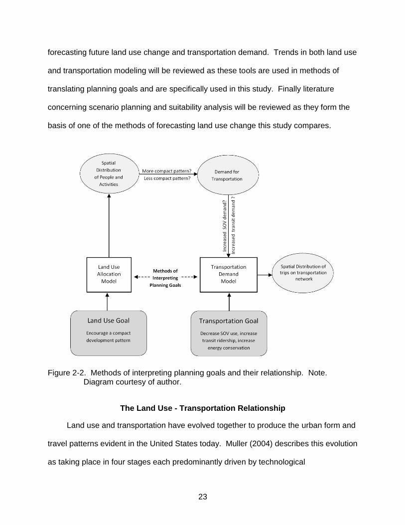
like increasing transit ridership may be achieved (Figure 2-2). The effectiveness of
methods used to translate, quantify, and represent planning goals thus also plays an
important role in the attainment of long-range planning goals and the coordination of
transportation and land uses.
Figure 2-1. Example of mutually supportive land use and transportation planning goals. Note. Diagram courtesy of author.
The following literature review addresses these two broad topics; the relationship
of land use and transportation, and methods used to represent land use and
transportation goals in long-range plans. Beginning with the land use and transportation
relationship the review will narrow its focus to literature relevant to methods of
23
forecasting future land use change and transportation demand. Trends in both land use
and transportation modeling will be reviewed as these tools are used in methods of
translating planning goals and are specifically used in this study. Finally literature
concerning scenario planning and suitability analysis will be reviewed as they form the
basis of one of the methods of forecasting land use change this study compares.
Figure 2-2. Methods of interpreting planning goals and their relationship. Note.
Diagram courtesy of author.
The Land Use - Transportation Relationship
Land use and transportation have evolved together to produce the urban form and
travel patterns evident in the United States today. Muller (2004) describes this evolution
as taking place in four stages each predominantly driven by technological

24
advancements that have enhanced human mobility. The following overview broadly
highlights this interaction between transportation and land use and provides some
historical background to the discussion that follows.
The Spatial Evolution of Urban America
Walking-Horsecar era (1800 – 1890)
The introduction of the horse-drawn streetcar in the mid 19th century enabled
middle-income city residents to move to the urban fringes away from the overcrowding
and pollution that accompanied the industrialization of American cities (Muller, 2004, p.
64-67). Prior to this transportation innovation the urban area was limited to the extent to
which people could comfortably walk resulting in the clustering of people and activities
within close proximity of each other (Muller, 2004, p. 64). The horse-drawn streetcars
moved along rails which slightly improved their speed compared to moving along
unpaved roadways, attracting city residents that could afford the fare the opportunity to
move to the narrow strip of land on the cities periphery (Muller, 2004, p. 66). Initially the
streetcars followed radial routes but the demand for housing on the urban fringe saw the
construction of cross-town lines and infill development soon followed.
Electric streetcar era (1890 – 1920)
The invention of the electric traction motor was to revolutionize mobility and Muller
(2004) considers it one of the most important innovations in US history. By attaching
motors to streetcars speeds of up to 15 miles- per-hour could be achieved bringing a
much wider area on the urban fringe into commuting distance to the city (Muller, 2004,
p. 67). As streetcar lines ran further away from downtown areas development along
them changed the overall shape of cities from a circular to a star-shaped pattern.

25
Commercial development occurred alongside trolley tracks with residential streets
forming a grid pattern in between lines (Muller, 2004, p. 67).
The relatively low fare charged by streetcar companies coupled with extensive
networks of lines increased mobility for city residents and resulted in a greater
separation of land uses as people could now live further from centers of commerce and
industry (Muller, 2004, p.69). Specialized land use zones quickly emerged with the
central business district becoming the predominant location for such activities. The
invention of the elevator also enabled greater clustering as buildings grew in height
further concentrating commercial development downtown (Muller, 2004, p. 69). The
later years of this era saw the introduction of electric commuter trains in larger cities
such as New York that either superseded the streetcar systems or in the case of new
cities such as Los Angeles were adopted outright (Muller, 2004, p. 69).
Recreational automobile era (1920 – 1945)
The advent of the automobile was to have the most drastic impact on urban form
beginning slowly in the interwar period. Initially restricted to the wealthy, Henry Ford‟s
mass production techniques quickly made the car an affordable mode of transportation
for the majority of Americans (Muller, 2004, p. 70). Many of the earliest roads were
constructed in rural areas where farmers badly needed better access to local services.
City dwellers initially used their cars for recreational trips but quickly came to realize
their potential for personal daily travel. As early as 1922 the number of car dependent
households had grown to 135,000 across 60 cities (Muller, 2004, p. 70). The increasing
mobility that cars provided caused an increase in possible commuting distances and
spurred further development on urban fringes and between suburban rail axes. The
subsidization of the streetcar system by home-building companies was no longer

26
necessary as potential new homeowners provided their own means of transportation.
The demise of the suburban transit system soon began and was heightened during the
Depression years of the 1930s (Muller, 2004, p. 71-72).
Freeway era (1945 – present)
In contrast to the preceding eras that were spurred by some innovation in
transportation technology, this period has been driven by a different force, the freeway.
Enabled by the massive highway-building building effort of the post-war economic
boom, the pattern of urban development rapidly dispersed as mobility increased along
the high-speed expressways that allowed even further separation of land uses (Muller,
2004, p. 75-81). Car ownership was no longer a luxury; it was a household necessity
for working, shopping and entertainment. Just as the streetcar system produced a
network-shaped development pattern, so too did the freeway system (Muller, 2004, p.
76); extending development into increasingly more distant locations and resulting in the
widely dispersed patterns of urban development common across the United States
today.
The regional advantage that city central business districts had in attracting
business and employment was mostly eliminated by the network of expressways that
now connected any location along its path (Muller, 2004, p. 76). Lower cost locations
for business along expressway routes attracted commercial, retail and light industrial
development to highway intersections in the outer city areas; creating suburban
downtowns which in turn attracted residential development (Muller, 2004, p. 79). With
the ever increasing distance and separation of land uses, mobility for most Americans
had become dependent upon car ownership and the ability of the road network to take
them to the places the needed to go.

27
Mobility and Accessibility – Key Concepts
The above overview highlights the affect transportation innovations have had on
urban form in the United States and the patterns of development that have evolved
within urban areas. Two key concepts emerge from this historical background that are
helpful in understanding the relationship between land use and transportation; mobility
and accessibility. The following section provides an overview of these concepts, so the
changing emphasis each has received in planning theory and practice may be better
observed.
At a very broad level the link between land use and transportation can be
understood in simple terms. Transportation can be described as the network of routes
taken to move from one location to another using various modes of transport (Meyer
and Miller, 2001, p. 128). How this network is organized is largely dependent on the
configuration of the land uses it serves as these dictate where people and the activities
they undertake are located and directly affects their mobility, or in other words their
ability to move from place to place. Similarly, land use patterns are influenced by the
transportation system which determines how accessible one location is to another
(Meyer and Miller, 2001, p. 128) and is dependent upon the available routes and modes
for travel.
As the above description highlights mobility and accessibility are two concepts
central to understanding the land use and transportation relationship. In this light
mobility can be seen as being principally a function of the characteristics of the
transportation network and the modes it employs, or more simply the means by which
people can travel. Accessibility however is linked to location and is characterized by
how easily a location can be reached using the transportation network as well as by the

28
number and type of activities a location offers and when these are available (Hanson,
2004, p. 5-6). Thus accessibility is dependent on mobility because it determines how
easily a location can be reached and perhaps more importantly by what modes.
Hanson (2004) points out that accessibility can be measured in different ways.
For example personal accessibility often refers to the number of activity sites within a
given distance of a person‟s home and how easily they can be reached, whereas
location accessibility refers to the number of activity sites within a given distance of a
specific place (p. 6). Both are measured in similar ways however there is an important
distinction between them. Measures of location accessibility treat all people within the
zone of measurement as being the same, so that those without access to a private
vehicle are considered to have the same accessibility as those who do (p. 6). Thus a
person living in walking-horsecar era town where people and activities were clustered
closely together would have had higher levels of personal accessibility than someone
living in a freeway era home without owning a private vehicle because the majority of
activity sites can only be reached by car. Although such measurements and examples
are overly simplified they do highlight the role mobility, and particularly available modes
of transportation, play in how accessible people and places are to each other.
The historical background of the spatial evolution of urban America highlighted
that as the demand for mobility increased the need for mobility increased
simultaneously as land uses became more segregated and people more car dependent.
In keeping with this demand, increasing mobility has been a paramount goal for
transportation planners who have often equated an increase in mobility with an increase
in accessibility (Hanson, 2004, p. 4-5). As Handy (2005) points out this planning

29
approach is problematic as it perpetuates a cycle of continually planning for mobility,
where increasing the capacity of road systems to reduce congestion and increase
mobility eventually leads to more travel, mounting congestion and a need to further
increase mobility (p. 11). While accessibility may be increased for those who own a car,
those unable to drive due to their age, disability or economic hardship are significantly
disadvantaged (p. 11). The likelihood of increasing transportation costs in the relatively
near future due to declining global oil reserves may create economic hardship and
declining accessibility for large numbers of people living in urban fringe areas where
driving distances are typically longer than average commutes.
Trends in Planning Approach and Research
Interest in understanding the relationship between land use and transportation is
not new. As early as 1930, research was undertaken to investigate the effect of a new
subway line on land values in surrounding areas (Meyer and Miller, 2001, p. 133). The
past several decades however have seen an increase in research interest in better
understanding the relationship. Meyer and Miller (2001) summarized 36 studies that
examined the land use and transportation relationship, spanning the years 1930 to
1997; 6 were from prior to 1970, 12 were from the 1970s, 3 from the 1980s, and 15 from
the 1990s. To substantiate whether this increase in studies represents an increase in
research interest in studying the relationship between land use and transportation, a
literature search was undertaken using the online ScienceDirect database. The
ScienceDirect database contains approximately 9.5 million journal articles and book
chapters from over 2,500 peer-reviewed journals and books (Elsevier, 2010). Several
different parameters regarding land use and transportation were queried and the results
are summarized in Table 2-1. The results of this literature search reinforce the review

30
undertaken by Meyer and Miller (2001) by highlighting that since 1970 research interest
has grown increasingly over the past four decades. Depending on the search
parameters used, the increase in the number of published journal articles and book
chapters on the topic of land use and transportation and related issues increased from
five to ten-fold between 1970 and 2010.
Table 2-1. Number of journal articles and book chapters resulting from literature search of ScienceDirect database
Title, Abstract or Keyword =
1961 to
1970
1971 to
1980
1981 to
1990
1991 to
2000
2001 to
2010
1970 to
2010 %
incr.
"land use" & "transportation" 2 67 70 129 398 494 "land use" & "transportation" & "transit" 1 18 22 42 134 644 "land use" & "transportation" & "density" 1 43 36 69 247 474 "land use" & "transp." & "accessibility" 0 19 25 35 108 468 "land use" & "transp." & "mobility" 0 8 11 35 105 1213 "land use" & "transp." & "VMT" 1 11 7 23 67 509
Note. The ScienceDirect online database was searched via the University of Florida Library system at http://www.sciencedirect.com.lp.hscl.ufl.edu/ on March 9, 2010. The search included all journals and books, from all sources and all subject areas.
The research trend demonstrated in Table 2-1 may be explained in the context of
changes to the land use and transportation planning process that began in the late
1960s with the introduction of several key federal policies that dictated a need for a
better understanding of the land use and transportation relationship. Table 2-2 lists
these policies and some of their key points that were to effect the transportation
planning process. The passage of these Acts collectively reflects changing American
attitudes towards their society and the environment.
Issues of social justice within urban areas came to the forefront of planning
discussions in the US during the 1960s and 1970s, with an emphasis on creating
redistributive policies that favored minorities and those under-represented in the

31
planning process becoming popular (Deka, 2004, p. 334). Urban unrest in many
American cities was the driving force behind this movement, with the Watts riot in Los
Angeles in 1965 typifying the tensions during this period. The McCone Commission
that investigated the Watts riot concluded that the social problems that led to the rioting
were in part due to a lack of adequate transportation services restricting the mobility and
accessibility of inner-city residents (Deka, 2004, p. 335). Three key policies reflect a
government response to these issues, the Federal-Aid Highway Acts of 1970 and 1973,
and the National Mass Transportation Assistance Act of 1974, all of which direct
government spending on mass transit. The observed increase in literature published on
the topics of land use, transportation, transit, density, accessibility and mobility (Table 2-
1) may be attributed to the introduction of these three pieces of legislation and the effect
they were to have on the planning process, spurring a need to better understand the
interrelationship of these topics.
The 1960s and 1970s was also the period at which environmentalism was at the
forefront of planning discussions, with environmental planning emerging as a profession
in its own right around this time (Deka, 2004, 345). Of greatest concern to
environmental planners was the protection of the natural environment from polluting
industries (Deka, 2004, 345). Such concern is reflected in the enactment of several
important pieces of legislation that were to have significant impacts on transportation
planning. They were the National Environmental Policy Act of 1969 (NEPA), the Clean
Air Acts of 1970 and 1977 (CAA) and the National Energy Act of 1978 (NEA). Each of
these acts was to place requirements on responsible agencies to monitor environmental
impacts of transportation investments.

32
Table 2-2. Selected federal policies related to urban transportation planning
Year Act Key Points
1969 National Environmental Policy Act (NEPA)
Req‟d preparation of env. Impact statements (EIS) for major federal actions – to include direct and indirect effects (present & future) - induced development impacts of h‟way projects are considered an indirect effect and must be forecasted
1970 Clean Air Act Amendments
Created Env. Protection Agency authorized to set ambient air-quality standards – req‟d development of state implementation plans (SIPs)
1970 Federal-Aid Highway Act Req‟d US Dept. of Transportation regulations to assure adverse economic, social and env. effects are fully considered in h‟way projects
1973 Federal-Aid Highway Act
Allowed expenditure of federal-aid h‟way urban systems money to be spent on mass transp. projects – allowed withdrawal of interstate segments and substitution of mass transit projects
1974 National Mass Transportation Assistance Act
Authorized federal operating assistance for urban transit systems
1977 Clean Air Act Amendments
Req‟d revisions to (SIPs) for areas not in attainment of national air-quality standards – SIPs were req‟d to develop transp. control plans to reduce mobile (from transp. sources) emissions
1978 National Energy Act
All phases of transp. planning and project development were to encourage fuel conservation – states req‟d to undertake conservation actions such as car-pooling programs
1990 Clean Air Act Amendments
Projected emissions associated with transp. projects and programs must be reconciled with the req‟d emission reductions of SIPs
1991 Intermodal Surface Transportation Efficiency Act
Req‟d consideration of 15 planning factors in metro transp. planning, relating to mobility and access for people and goods, system performance and preservation and environment and quality of life
Note. Adapted from “Urban Transportation Planning”, by Meyer and Miller, 2001, pp. 619-629.

33
The substantial air quality problems being experienced in many US cities during
the 1960s and 1970s led to the amendments of the Clean Air Act (see Table 2-2) which
had originally been passed in 1955 in response to growing concerns about the health
problems associated with vehicle emissions (Wachs, 2004, 141). Requirements to
meet air-quality standards placed greater emphasis on understanding how the
interaction between land use and transportation influence travel behavior, the major
driver of the demand for mobility and automobile use. Increased interest in transit as a
means to reduce congestion, improve air quality and save energy is reflected in the
enactment of the Federal-Aid Highway Act amendments of 1970 and 1973 and the
National Mass Transportation Assistance Act of 1974. Seen together, the enactment of
the federal policies from the 1960s and 1970s listed in Table 2-2 help explain the
increased research interest during that period that the literature search details in Table
2-1 depicts.
The early 1990s saw two influential acts of federal legislation also have marked
affects on how transportation investments were planned. The Clean Air Act of 1970
(CAA) had already brought transportation planners into the sphere of environmental
planning by linking the automobile to the nation‟s air pollution problems (Hanson,
2004:24). The 1990 Clean Air Act Amendments (CAAA) strengthened that link by
requiring the integration of clean air planning and transportation planning at the regional
level, mandating that transportation programs must meet air quality standards. The
need to forecast future travel demand, or predict vehicle-miles of travel (VMT), as a
means of assessing impacts to air quality for a transportation project thus became a
legislative requirement for local, regional and state transportation planning agencies.
34
One particular conformity rule (40 CFR 93.122[b][1]) required Metropolitan Planning
Organizations (MPOs) to adopt some kind of land use forecasting model or committee
that could account for the regional impacts of transportation plans on land development
(Johnston, 2004:119).
Similarly the 1991 Inter-modal Surface Transportation Efficiency Act (ISTEA) had
an impact on the quantitative assessment of transportation plans. The Act required
State Departments of Transportation (DOTs) and MPOs to have coordinated long-range
transportation plans (LRTPs) and transportation improvement programs (TIPs) that
were now to include as considerations land use, inter-modal connectivity and transit
service enhancement methods (Bureau of Transportation Statistics, unknown). In
particular, the requirement to consider land use in transportation planning would compel
agencies to better understand the relationship between the two.
When analyzed in conjunction with an overview of several key federal policies
relating to urban transportation (Table 2-2), the increased research interest observed in
the literature search (Table 2-1) suggests that a trend exists that reflects firstly a gap in
knowledge about how land use and transportation interact, and secondly a recognition
that a better understanding of it may be necessary to address the social and
environmental problems urban planners seek to resolve.
Meta-Analysis of Selected Literature Reviews
The two-fold increase in literature published on topics relating to land use and
transportation between 1990 and 2010 (Table 2-1) can be furthered explained in the
context of two global concerns that have a direct relevance to these topics; adverse
climate change due to global warming and uncertainties about future global oil supplies.
For a country like United States, which had over two billion cars in 2005 (United Nations

35
Economic Commission for Europe, 2008), these issues have serious implications for the
future mobility of a population who depend almost entirely on personal vehicles for
transportation. According to the US Environmental Protection Agency (EPA)
transportation is the second largest contributor to greenhouse gas (GHG) emissions
(US EPA, 2009). Transportation is also the largest consumer of petroleum products in
the United States according to the US Government Accountability Office (GAO) (p. 9)
which also reported in 2007 that global oil supplies are predicted to begin declining
within the next 30 to 40 years (p. 4). Strategies to reduce GHG emissions and the
consumption of petroleum products involve technological advancements to improve fuel
efficiency in cars, increased use of alternative energy sources, and reducing fuel
consumption. A reduction in fuel consumption, or VMT, has thus become a serious goal
of transportation planners in the past decade and provides the motivation for many of
the more recent research studies in land use and transportation.
In response to the recognized need to reduce fuel consumption the US
Department of Energy requested the Transportation Research Board (TRB), a private
non-profit institution that provides services to the government and public on
transportation matters (TRB, 2010), to undertake a study into the relationships between
VMT, development patterns and energy consumption (TRB, 2009, p. xi). This report and
the literature reviews of three other authors will be examined and a meta-analysis of
their findings will be reported in the remainder of this section. Table 2-3 details the
authors being reviewed, the year of their publication, and a broad summary of their
findings.
36
Badoe and Miller (2000)
In their study into the transportation-land use interaction, Badoe and Miller (2000)
identify the current state of knowledge with a particular focus on potential policy impacts
and also to identify gaps in the knowledge to guide future research (p. 236). Their
overall goal is to generate discussion for the development and application of integrated
models of land use and transportation (p. 236). Their empirical review focused mostly
on studies published after 1994 and analyzed the data based on two categories;
literature on the impact of urban form on travel behavior, and literature on the impact of
transportation (transit in particular) on urban form (p. 236).
Their review of the literature on the impact of urban form on travel behavior was
further categorized according to five main topics; residential density, accessibility,
neighborhood design, car ownership, and transit supply. Their analysis of findings
related to residential density was that the evidence was very mixed. Although some
studies showed that density had a significant effect in increasing transit use or
decreasing VMT, other studies found that the significance decreased when other factors
such as socio economic status and car ownership were considered (p. 248).
Findings related to accessibility were also mixed due to the fact that most studies
assess its importance relative to other factors and these factors varied across the
studies (p. 251). Most studies overlooked the significance of connectivity (of the road
network) which is often a major determinant of accessibility (p. 252). Studies
concerning neighborhood design provided a mixture of findings with the principal flaw of
most relating to the scale of their investigation. Because the geographic range of
activities for most people extends far beyond the neighborhood scale the complex
37
relationships between neighborhoods and regions may be overly simplified by this type
of analysis (p. 253).
Findings related to car ownership were consistent across the studies reviewed,
with the common result showing that higher residential densities are associated with
lower car ownership and households with fewer cars tend to use transit more than those
with more cars (p. 253). Few studies investigated the impact of transit use on urban
form but those that did showed transit played a significant role in explaining mode
choice, VMT, and effects of residential density (p. 254).
Studies investigating the impacts of transit on urban form focused mostly on rail
transit (subway, light and commuter rail) and resulted in variety of findings. Most
studies concentrated on transit‟s influence on land values with the overall conclusion
that rail development facilitates rather than generates new development (p. 259).
The overall finding of the literature review by Badoe and Miller (2000) was that
there was a wide variety of conclusions being drawn across various studies about the
strengths and weakness of the relationship between land use and transportation (p.
260-261). Methodological and data weaknesses were largely responsible for a lack of
clarity with respect to potential policy impacts. They conclude that an integrated urban
model that accounts for all actors and factors in the urban system should be an area for
further research (p. 261).
Ewing and Cervero (2001)
In their study of travel and the built environment Ewing and Cervero (2001) set out
to provide a generalization across a large number of previous studies into the
relationship between travel behavior and urban form. Many existing studies focus
mainly on research findings without elaborating on methodological details making it
38
difficult to assess their reliability and validity (p. 87). Ewing and Cervero aimed to
collectively assess the body of literature with a focus on providing more detail of how
studies were done so differences between them could be identified (p. 87). They take
an empirical approach by reviewing 46 studies focusing on how each explains four
types of travel variables; trip frequencies, trip lengths, mode choices, and cumulative
person-miles traveled or vehicle-miles traveled or vehicle-hours traveled (p. 87). The
studies are categorized according to the general characteristics of the built environment
they investigate; neighborhood and activity center designs, land use patterns,
transportation networks, urban design features, and composite transit- or pedestrian-
oriented design indices. A table for each category summarizes the studies it includes
and the land use-transportation relationships identified.
Studies that compared neighborhood and activity center designs were furthered
categorized as being contemporary, or traditional, car or pedestrian oriented, and urban
or suburban (p. 88). Across all these sub-categories of the built environment trip
frequencies differed very little, with socio-economic characteristics of households being
a major determinant. Although evidence was limited trip lengths appeared to be shorter
in traditional neighborhoods which would be expected due to the finer land use mixes
and grid networks characteristic of this type of development (p. 88). Walking and transit
use are also more prevalent in traditional settings but this could be due to self-selection;
those who prefer these modes choose to live in settings where it is possible (p. 88).
Studies that tested land use variables were far more prevalent than any other type
of study (p. 92). These have generally focused on residential and employment
densities, measures of land use mix, and measures of accessibility that reflect the

39
number of attractions with a specific distance of households (p. 92). Overall these
studies showed vehicular travel is mainly a function of regional accessibility, even when
the effects of local density and land use mixed are controlled. This indicates that higher
density, mixed use developments that are regionally isolated from other activity sites
may be of only modest regional travel benefit (p. 92). Trip frequencies were mostly
dependent upon socio-economic characteristics rather than land use variables (p. 92).
Mode choice was the travel variable that was most affected by local land use variables
with transit use being firstly dependent on local densities and secondly on land use mix,
and walking equally dependent on both (p. 92). Employment densities at trip
destinations was possibly more important at destinations than population densities at
origins for both transit and walking modes, meaning the preoccupation with residential
densities by proponents of transit-oriented development (TOD) may be misguided (p.
92). Many studies focused on density but whether the impact of density on travel
behavior is due to density itself or other variables is still not determined (p. 92-93).
Many transportation network variables can affect travel times by different modes
and can potentially affect travel decisions. Some include street connectivity, routing
directness, block size and sidewalk continuity (p. 100). Walking and transit access are
improved by grid patterns of streets but so is car access, so it is difficult to determine
which mode gains the most advantage from this configuration (p. 100). The
attractiveness of network types to particular modes depends on design and scale, with
grid patterns of narrow streets being more attractive to walking than car travel (p. 100-
101). Evidence showing a relationship between network design and travel are mixed so
firm conclusions could not be drawn (p. 101).

40
There were relatively few studies that tested urban design variables such as
crosswalks, sidewalks, parking supply and building orientation. Individually design
variables were seldom significant in impacting travel and those that appeared to such as
crosswalks near bus stops more likely were capturing some other unmeasured feature
of the built environment (p. 102). Collectively however urban design variables may
have some impact on travel. Studies of composite land use design features, those
focusing on transit or pedestrian-oriented design may show an interactive effect
between land use and transportation variables (p. 106). For example a high traffic area
with no sidewalks may lower accessibility whereas individually each of these factors has
little impact on travel (p. 106). Different studies used different composite measures with
some being more subjective than others, and some arbitrarily weighting variables and
others using statistical estimates to base weights according to their associations with
other variables (p. 106). Overall these disparate approaches to measuring, for example
transit friendliness or walking quality, have resulted in inconclusive results about the
relationship between composite design measures and the impact on travel (p. 106).
Generalizing across all the studies Ewing and Cervero conclude that trip
frequencies are mainly a function of socio-economic characteristics and then the built
environment, whereas trip lengths are a function of the reverse, firstly the built
environment and then socio-economic characteristics (p. 106). Mode choices are
dependent equally on both the built environment and socio-economic characteristics,
and vehicle or person miles traveled is most significantly affected by the built
environment (p. 107). The authors call for more transparent ways of reporting results of
studies on the relationship between land use and transportation and suggest as an
41
example an approach involving the measurement of the elasticity of VMT in relation to
land use and design variables (p. 107).
Handy (2005)
Handy (2005) sets out to test four often stated propositions of advocates for Smart
Growth approaches to planning that encourage urban development to be compact in
form, pedestrian friendly, accessible to transit and diverse in land uses (p. 147-148).
Handy reviews the studies of the relationship between land use and transportation to
uncover evidence that support the following propositions:
Building more highways will contribute to sprawl (p. 148)
Building more highways will lead to more driving (p. 148)
Investing in light rail will increase densities (p. 148)
Adopting new urbanism design strategies will reduce automobile use (p.
148),
With regard to the first proposition, evidence from the literature shows that
highway building does contribute to sprawl by influencing where growth occurs. Rather
than generating growth the research showed the effects are redistributive and overall
highway building influences where and at what densities growth occurs (p. 152).
Handy points out that while this appears to be true the converse is probably not. In
other words, not building highways will not slow sprawl, (p. 153). For example the
expectation of building a highway may be sufficient to induce new development.
Studies in the 1990s showed that, with regard to the second proposition, a
statistically significant relationship between increasing highway capacity and increased
travel demand existed (p. 154). Their results suggested that in economic terms the
42
travel time savings gained by increased road capacity caused an increase in travel
consumption (p. 154). However more recent studies using disaggregate approaches
and modeling techniques that better identify causalities suggest that the earlier studies
overestimated impacts and that highway building has only a limited affect on induced
travel demand (p. 154). Handy concludes that it has yet to be concluded as to whether
or not increasing highway capacity contributes to a growth in VMT (p. 154).
Just as the literature showed that highway building had a redistributive rather than
a generative effect on new development, the evidence in support of the third proposition
that light rail transit (LRT) will increase densities was similar (p. 156-157). The
literature did show however that under certain circumstances LRT may increase
densities, although it was not assured. These circumstances included significant growth
occurring in a region, a transit system that significantly increases accessibility, station
locations sited in areas conducive to development, and supportive land use policies and
capital investments (p. 159).
Handy points out that with regard to the fourth proposition that new urbanism
design strategies will reduce car use, researchers are challenged by the difficulty of
separating out the relative importance of socio-economic characteristics from the effects
of design (p. 161). The problem of self-selection, that people who prefer to drive less
seek out neighborhoods where it is possible to drive less, was addressed by a few
researchers but overall they failed to capture people‟s motivation for choosing the
residences (p. 162). Handy concludes that new urbanism design strategies may reduce
car use by a small amount by addressing the unmet needs of these wanting to live in
such neighborhoods (p. 162).
43
In conclusion Handy finds that for all the propositions questions remain as to how
strong the link is between land use and transportation and the direction of causality in
factors affecting the relationship (p. 164. She summarizes her conclusion as follows:
New highway capacity will influence the location of growth (p. 163)
New highway capacity may slightly increase travel (p. 163)
LRT can encourage higher densities under certain conditions (p. 163)
New urbanism strategies make driving less easier for those wish to drive
less (p. 163).
Transportation Research Board (2009)
The TRB report investigating the effects the built environment has on driving
devotes a chapter to a review of the literature on the impacts of land use patterns on
VMT and draws on the studies covered by the three literature reviews summarized
above, Badoe and Miller (2000), Ewing and Cervero (2001) and Handy (2005) (p. 39).
As such focus here will be given to the more recent studies, published after 2005, that
TRB investigates in their literature review.
In an effort to account for the problem of self-selection, some of the more recent
studies have carefully controlled for a wide range of socio-economic variables to test for
their effect on VMT (p. 43). While some have investigated the effect of only one factor,
density, on VMT, a thorough study by Bento et al. (2005) controlled for several
variables, population centrality, jobs-housing balance, city shape, road density and rail
supply and found each to have a significant albeit statistically small effect (p. 43). The
work of Bento et al. suggests however that when these factors are considered
simultaneously VMT could be lowered by as much as 25 percent (p. 46).

44
The effects of TOD on travel were investigated by several recent studies which
indicate that transit supply and accessibility in combination with land use are important
variables affecting mode choice and thus VMT (p. 46). Of particular importance
appears to be the location of a TOD within a region because this affects its accessibility
to desired locations, as does the quality of connecting transit services which were found
to be more influential in travel patterns than the actual design characteristics of the TOD
itself (p. 46). With regard to land use and design features, proximity to transit and
employment densities at trip ends appears to have a stronger influence on transit use
than urban design features to enhance walkability and land use factors such as mixed
uses and increased residential densities (p. 47).
The literature review of this report concludes that few of the studies consider the
potential a group of policies that combine increased density with higher concentrations
of employment, improved accessibility to a variety of land uses and a good transit
network can have on reducing VMT (p. 31). The authors consider two case studies
where such a combination of factors has been fostered by different policy approaches,
Portland Oregon, and Arlington County Virginia (p. 51-53). They conclude that the
dramatic changes to the built environment and travel patterns require a significant
political commitment and substantial transportation investments over a long period of
time which will be challenging for many metropolitan areas (p. 54).
45
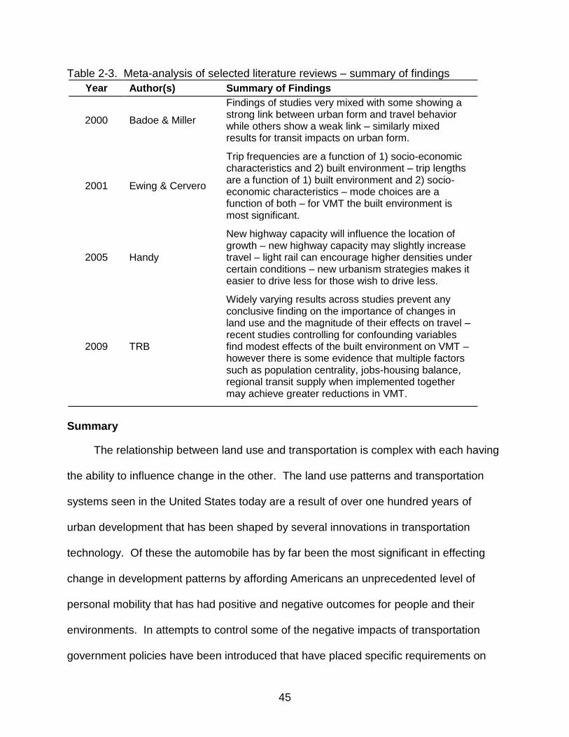
Table 2-3. Meta-analysis of selected literature reviews – summary of findings
Year Author(s) Summary of Findings
2000 Badoe & Miller
Findings of studies very mixed with some showing a strong link between urban form and travel behavior while others show a weak link – similarly mixed results for transit impacts on urban form.
2001 Ewing & Cervero
Trip frequencies are a function of 1) socio-economic characteristics and 2) built environment – trip lengths are a function of 1) built environment and 2) socio-economic characteristics – mode choices are a function of both – for VMT the built environment is most significant.
2005 Handy
New highway capacity will influence the location of growth – new highway capacity may slightly increase travel – light rail can encourage higher densities under certain conditions – new urbanism strategies makes it easier to drive less for those wish to drive less.
2009 TRB
Widely varying results across studies prevent any conclusive finding on the importance of changes in land use and the magnitude of their effects on travel – recent studies controlling for confounding variables find modest effects of the built environment on VMT – however there is some evidence that multiple factors such as population centrality, jobs-housing balance, regional transit supply when implemented together may achieve greater reductions in VMT.
Summary
The relationship between land use and transportation is complex with each having
the ability to influence change in the other. The land use patterns and transportation
systems seen in the United States today are a result of over one hundred years of
urban development that has been shaped by several innovations in transportation
technology. Of these the automobile has by far been the most significant in effecting
change in development patterns by affording Americans an unprecedented level of
personal mobility that has had positive and negative outcomes for people and their
environments. In attempts to control some of the negative impacts of transportation
government policies have been introduced that have placed specific requirements on

46
planning, implementation and management of the transportation system. The literature
reveals that while research into better understanding the land use and transportation
relationship has been influenced by government policies and public concerns about
uncontrolled urban development, recent global concerns about climate change and
crude oil shortages have lead to even more concerted research in this area. While
much has already been learned the literature shows that there is still a considerable gap
in the knowledge of how land use and transportation systems should be managed in
order to avoid negative social, economic and environmental impacts and still provide an
adequate level of mobility and accessibility for everyone.
Transportation and Land Use Modeling
The use of computer models in the preparation of transportation plans has been
common practice since the 1960s following the introduction of Federal Aid Highway Act
of 1962, which required all federally funded highway projects to be based on a
continuing, comprehensive and cooperative planning process involving state and local
planning agencies (Meyer and Miller, 2001, p. 619). An integral part of that process is
the forecasting of transportation demand and how that will impact the transportation
network. This is typically performed using computer models, as are forecasts of land
use change that determine the location of people and activities upon which
transportation demand is estimated. Both model types form the basis of a framework
generally used by transportation planners in the creation of long rang transportation
plans. This section will review the transportation and land use models commonly used
in this framework and how that has changed over time, with special attention focused on
the model types used in this study.

47
Transportation Modeling – The Four Step Model
A model can be described as a simplification or abstraction of a real world system
that can be used to test what might happen to the system if changes occur within it
(Meyer and Miller, 2001, p. 256). In the history of transportation planning one model
type has been dominant since the early 1950s (McNally, 2007b, p. 35 -36). The urban
transportation modeling system, most commonly referred to as the four-step model
(FSM) was originally developed for evaluating large-scale infrastructure projects at the
regional and sub-regional scale (McNally, 2007b, p. 38). Despite its limitations which
will be reviewed later it remains the primary tool used for forecasting future
transportation demand and performance (McNally, 2007a, p. 54).
Overview
The FSM is made up of four sub-models that use data inputs concerning the
characteristics of the transportation system and the characteristics of the land use
system (Figure 2-3). The transportation system is represented graphically in the model
as a network of links and nodes which have information such as length, speed, and
capacity for links, and turn prohibitions and penalties for nodes associated with them
(McNally, 2007b, p. 38). The land use system is aggregated to traffic analysis zones
(TAZs) containing socio-economic and land use data typically comprised of census data
and/or data collected from household and workplace travel surveys, vehicle intercept
station surveys or onboard transit surveys (Meyer and Miller, 2001, p. 191-199). The
data typically reflects activities performed over a 24-hour period and includes activity
type, location, duration, and arrival and departure times (McNally, 2007b, p. 40).
Following is an overview of the four sub-models that typically make up the FSM.
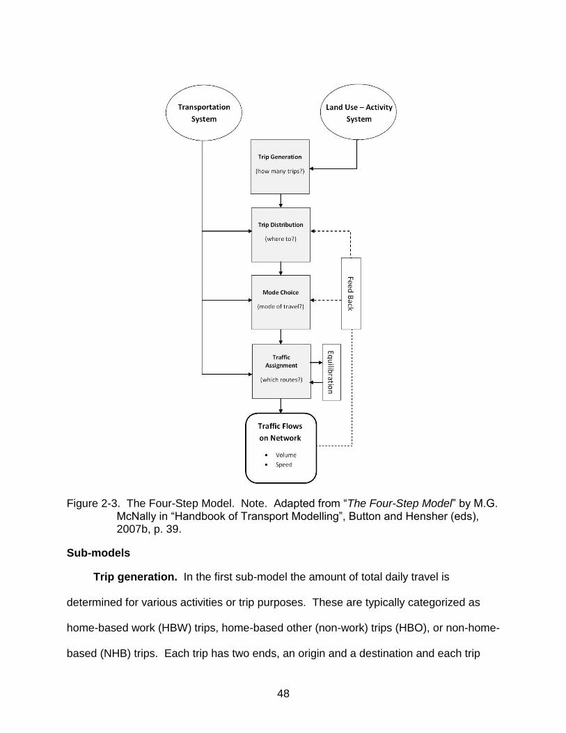
48
Figure 2-3. The Four-Step Model. Note. Adapted from “The Four-Step Model” by M.G.
McNally in “Handbook of Transport Modelling”, Button and Hensher (eds), 2007b, p. 39.
Sub-models
Trip generation. In the first sub-model the amount of total daily travel is
determined for various activities or trip purposes. These are typically categorized as
home-based work (HBW) trips, home-based other (non-work) trips (HBO), or non-home-
based (NHB) trips. Each trip has two ends, an origin and a destination and each trip
49
end is classified as a production or an attraction. Productions are considered to be the
home-end of a home-based trip, or the origin of a NHB trip, while attractions are the
non-home end of a home-based trip, or the destination of a NHB trip (Meyer and Miller,
2001, p. 271). Separate models are used to define productions and attractions using
socio-economic data at the TAZ level. For the calculation of productions data such as
household income, size and employment, car ownership, residential densities and
distance to major activity centers are used. Workforce data such as the number of
employees, floor-space areas and accessibility to workplaces are used for the
calculation of attractions (Meyer and Miller, 2007, p. 271). The production and
attraction models basically calculate a measure of attractiveness for each TAZ which
serves to scale the trips for the next stage of the modeling process, trip distribution.
Where certain land uses generate untypical activities within a TAZ, such as a university
or hospital, special generator factors are included in the production and attraction
models to account for this activity (McNally, 2007b, p. 43).
Trip distribution. The objective of this sub-model is to distribute or connect the
zonal trip ends, the productions and attractions estimated for each zone in the trip
generation model, in order to predict the flow of trips from production zones and to
attraction zones (Meyer and Miller, 2001, p. 278). While there are many types of trip
distribution models, the most commonly used type is the gravity model. This type of
model estimates a travel impedance or friction factor (in terms of travel time or cost)
between two zones as a function of both the land use and transportation systems
characteristics (McNally, 2007b, p. 45). The transportation model used in this study, the
Central Florida Regional Planning Model (CFRPM) follows the Florida Standard Urban

50
Transportation Model Structure (FSUTMS) which specifies the use of a gravity model
for calculating trip distribution (Gannett Fleming, unknown, p. 45). In this gravity model
the desirability of traveling to a zone is directly related to its potential as a destination
based on the activities within that zone, and is inversely related to the spatial separation
(friction factor) between production and attraction zones (Gannett Fleming, unknown, p.
45). The final stage of trip distribution involves calibrating the model to the observed
data and often involves the manual adjustment of friction factors so a best-fit can be
made between the observed and estimated trips (Meyer and Miller, 2001, p. 280).
Mode choice. The purpose of the this sub-model is to factor the trip tables from
the trip distribution model to produce trip tables specific to each mode being modeled
(McNally, 2007b, p. 48). The most commonly used model type for this step is the
nested logit model, which is used in the CFRPM. Zone to zone person-trips are
allocated by trip purpose across the various modes and coefficients are used that
quantify the sensitivity or elasticity of each mode choice to changes in service (Gannett
Fleming, unknown, p. 71).
Traffic assignment. In the final sub-model the predicted flows between origin-
destination pairs for each mode are assigned to actual routes on the transportation
network. In determining route selection most models assume that individuals seek out
the most cost effective route, in time or money. The CFRPM employs an equilibrium
technique that runs several iterations of a minimum-path capacity constraint assignment
with travel time delays for each iteration being incorporated into subsequent ones
(Gannett Fleming, unknown, p. 77). The final result of this model step is an estimate of
trip volumes and speeds on the network links. In the CFRPM highway and transit trips

51
are assigned in two different sub-models. The outputs from the highway assignment
include statistics on the number of lane and system miles, VMT, VHT (vehicle-hours
traveled), as well as original and congested speeds. The transit assignment outputs
include transit boards by mode, route and operator, as well as boarding and departure
statistics for each stop by route (Gannett Flemming, unknown, pp. 85 – 88).
Once the model is calibrated to reflect observed data it can be run for future year
estimates based on projected population and employment data and new land use
configurations. This study involves the modeling of three future land use scenarios
using the CFRPM.
Limitations of the FSM. An often cited criticism of the FSM is that it was
originally designed for evaluating large-scale highway projects and is policy sensitive
only with regard to major capacity improvements (McNally, 2007a, p. 54). As such the
FSM is not considered to be very effective in analyzing policy sensitivity because it fails
to adequately capture the complexities of travel, particularly at smaller scales. The FSM
focus on trips rather than activities results in the two not being linked during the
modeling process which is problematic because it is the underlying activity behavior that
generates trips (McNally, 2007a, p. 55). Also the FSM does not reflect temporal
constraints and other dependencies of activity scheduling such as trip-chaining,
meaning the sequencing of several trips to maximize time and cost savings (McNally,
2007a, p. 55). These limitations, among others, have led to continued research and
development of alternative modeling approaches.
Alternative approaches to the FSM. The FSM is an aggregate level model,
meaning it uses zonal data to model predictions about individual trips. An alternative
52
method is the disaggregate approach that begins by simulating the decision process of
individuals and summing them up to calculate aggregate travel demand (Meyer and
Miller, 2001, p. 290). Often referred to as discrete choice models, these typically are
based on the assumption that trip makers always seek to maximize utility, that is, they
rank trips according to their relative desirability, time/money cost, comfort and/or
convenience (Meyer and Miller, p. 290). Discrete choice models may utilize different
concepts to assume how trip decisions are made, such as random utility or nested logit
models like those commonly used in the mode choice step of the FSM.
Activity-based models are another approach which seeks to account more for the
behavioral aspects of trip making decisions. Models of this type typically fall into two
broad categories, econometric models and hybrid simulation models (Meyer and Miller,
2001, p. 306). Econometric models contain systems of equations that calculate activity-
travel choices as probabilities of possible outcomes or decisions. Hybrid simulation
models typically consist of rule-based algorithms that attempt to replicate actual
decision making processes (Meyer and Miller, 2001, pp. 301-307).
Integrated land use and transportation models are another approach to improving
the predictive capabilities of travel demand forecasting. Such an approach involves the
creation of feedback mechanisms between both model types within a modeling
framework which acknowledges the influence that land use, or human activities, has on
travel behavior, which determines the transportation network and in turn influences the
location and intensities of land uses (Miller et al., 1998, p. 1). Different land use models
and how they have been incorporated into the transportation modeling framework will
be discussed in more detail in the following section.

53
Land Use Modeling
At the basis of integrated land use and transportation modeling frameworks is the
idea that the relationship between the two can be simulated in a way that meaningfully
represents reality. Since the late 1950s a number of theoretical frameworks have been
developed by researchers that have significantly influenced the current research in land
use and transportation modeling (Iacono et al., 2008, p. 323). In a broad way these
frameworks can be categorized into three main areas, spatial interaction models,
econometric models and micro-simulation models.
Model types and operational characteristics
Spatial interaction models. Many early land use models employed the theory of
gravity to explain the distribution of people and activities across regions. In 1964 Lowry
was the first to use a gravity model as a basis for explaining the spatial interaction of
regions and their land uses (Iacono et al., 2008, p. 325). The main assumption of
gravity models is that the larger a city or region the greater its ability to attract
population, employment and commerce (Koomen et al., 2007, p. 7). A large number of
spatial interaction models have been developed over the past four decades that
continue to use gravity theory. One of the two methods of forecasting future land use
compared in this study uses a spatial interaction model based in gravity theory to
allocate projected population and employment growth. It will be reviewed in more detail
in the Chapter 3.
Econometric models. Models that employ econometric frameworks generally
contain two model types to predict locations of population, employment, commercial
activities and at times transportation flows. These models typically contain land market
and regional economic sub-models models which form the model‟s foundation. A wide
54
variety of models have developed using this framework, with many using different
theories to explain spatial distributions and actor behaviors. Random utility theory and
discrete choice theory are two methods used to improve the capabilities of these
models to simulate individual behavior which has resulted in improved measures of
accessibility and travel demand forecasting (Iacono et al., 2008, p. 328-331).
Micro-simulation models. As the name infers, micro-simulation models attempt
to model at a much finer resolution than the other model-types. They focus on the level
of the individual and typically include all the actors who influence land use changes.
Although some econometric models incorporate individual behavior they differ from
micro-simulation models in the way they estimate these behaviors. Rather than using a
cross-sectional or average of a population or market to estimate an individual behavior,
micro-simulation models take a bottom-up approach and estimate the behavior of
populations and markets based on the cumulative behavior of individuals (Koomen et
al., 2007, p. 12). Like econometric models, micro-simulation models employ a variety of
theories to explain the location of people, activities and commerce, including random
utility, discrete choice, multi-agent rule-based, and cellular automata approaches to
name a few (Iacono et al., 2007, pp. 332-335).
Operational characteristics. Apart from theoretical differences, models can also
differ by their operational characteristics. For example, a model may be characterized
as static, meaning it calculates a set of circumstances at a given point in time; or
dynamic, meaning it contains intermediate time steps that become beginning points for
subsequent occurrences (Koomen et al., 2007, p. 3). The variety of theoretical and
operational characteristics used to describe models often makes it difficult to categorize

55
them into uniform groups. The three frameworks described above however are a
starting point to understanding land use modeling and provide a wide context within
which the following meta-analysis of literature reviews can be analyzed.
Meta-analysis of selected literature reviews
Four literature reviews on land use models used in transportation modeling
frameworks were selected for analysis to determine whether any trends in the literature
could be observed. The selection of reviews was based on several criteria. As the
United States and Florida in particular are the locations of the study area for this
research, literature reviews that were relevant to both these geographic regions were
selected. To offer an international perspective it was also considered important to
include at least one review from outside the United States. Additionally, it was also
considered important to include reviews that were written from an academic or
theoretical standpoint, as well as reviews that aimed to fulfill practical purposes or
specific project goals, and to focus on most recently published works. Table 2-4 lists
the reviews by region, year, author and title.
Table 2-4. Selected literature reviews for meta-analysis of land use models
Region Year Author(s) Title
USA 1998 Miller, Kriger and Hunt Integrated Urban Models for Simulation of Transit and Land-Use Policies
USA 2000 U.S. Environmental Protection Agency
Projecting Land-Use Change: A Summary of Models for Assessing the Effects of Community Growth and Change on Land-Use Patterns
FL 2006 Zhao and Chung A study of alternative land use forecasting models
KOREA 2006 Chang Models of the Relationship Between Transport and
Land‐use: A Review
In the literature models are typically characterized by the different methodologies
they employ. Often models use multiple methodologies which can make categorization
56
difficult. In this meta-analysis the method used to categorize model types is the same
as that used in the literature review by Zhao and Chung (2006) which reviews the
largest number of models of all the selected reviews. Their approach was to classify
models based upon the methodology most emphasized by each model (Zhao and
Chung, 2006, p.3). A table listing these categories and which models were reviewed by
each author is listed in Appendix A.
Model strengths and weaknesses. In each of the selected literature reviews the
authors assess the strengths and weaknesses of each model type. Appendix B
provides a table summarizing these by author and model type. Over the time period
covered by these literature reviews (1998 to 2006) there appears to be a trend toward
favoring the more dynamic and disaggregate model types capable of a finer spatial
resolution, over the static and aggregate ones which typically have much coarser spatial
resolution. Disaggregate models attempt to simulate the behavior of individuals then
make assumptions about the behavior of large groups such as markets or populations.
Conversely, aggregate models simulate the behavior of markets or populations and
make assumptions about the behavior of individuals. Additionally, a model is
considered to be dynamic if the outputs of an earlier iteration of the model form part of
the inputs of subsequent iterations, in a way that reflects the cyclical nature of
transportation and land use. Static models on the other hand are not cyclical and
require a stepped process to occur if a feedback is required between iterations of the
model.
With the exception of the review by Zhao and Chung (2006) the literature reviews
did not intend to identify a particular model or type that is superior to the rest. In all of

57
the reviews however strengths and limitations are mentioned for the majority of model
types. When these factors are summarized (Appendix B) a general trend appears that
correlates with a characterization of the aggregate and static model types being limited
by those factors (i.e. by being static and aggregate), and the disaggregate and dynamic
model types as being strengthened by those characteristics (i.e. by being dynamic and
disaggregate). In addition, the majority of models reviewed in the earliest study by
Miller et al. (1998) were static and aggregate (spatial interaction and spatial input/out
models), with only one dynamic and disaggregate model (UrbanSim a micro-simulation
model) being reviewed. The more recent study by Zhao and Chung (2006) reviewed
the most models, including the largest number of dynamic and disaggregate models of
all the literature reviews, finding those to be the least limited of all model types.
Observed trend in the literature. A trend that favors the dynamic, disaggregate
model types over the static, aggregate ones has been recognized by others (Johnston
2004, Waddell 2004, Iacono et al. 2008, and Koomen et al. 2007) who have put forth
explanations for this development. The literature suggests that two influential factors
have contributed to this trend, firstly two key federal policies concerning the
environment and transportation, and secondly the emergence of Smart Growth
initiatives. The influence that the CAAA (1990) and the ISTEA (1991) had on the land
use and transportation planning process has already been discussed in an earlier
section, Trends in Planning Approach and Research, so only the topic of Smart Growth
initiatives will discussed here.
Smart Growth Initiatives. Beginning in the mid 1980s with increasing numbers of
states in the US overhauling their growth management legislation in an attempt to

58
combat sprawling development patterns (Weitz, 1999, p. 268), consensus within and
outside the planning community was building in support of a new approach to land use
planning. Although the interdependent nature of land use and transportation had long
been recognized (Kelly, 1994, p. 129) the idea that transportation investments might be
used as a tool to manage growth in a „smarter‟ way was just beginning to be realized
(Knaap, unknown, p. 12). The passage of ISTEA in 1991 led the US EPA to create the
Urban Economic Development Division (UEDD) which formed the Smart Growth
Network, to provide funding to a variety of Smart Growth projects (Knaap, unknown, p.
9).
Of the many principles that characterize Smart Growth development, three stand
out as most relevant to this study. By advocating mixed land uses, a provision of a
variety of transportation choices, and directing development toward existing
communities, Smart Growth initiatives have changed the way in which transportation
planners have traditionally viewed land use and development. Until this time
transportation planners and the land use models they used assumed land use change
resulted in changed transportation demands but that the transportation system itself did
not influence land use change (Borning, 2006, p. 2). These particular Smart Growth
concepts introduced a new level of complexity to travel demand modeling, and in turn
land use change forecasting, that highlighted the spatial, temporal and behavioral
limitations of the earlier models. The trend towards more dynamic and disaggregate
model types identified in this meta-analysis can be seen as an outcome associated with
the rise of Smart Growth initiatives.

59
Criticisms of complex models. The more complex models favored in the trend
observed by this review are not without some criticisms and drawbacks. Their
complexity often requires expert technical assistance for their implementation and
operation, making them potentially expensive and not accessible to those who may
benefit from them most, in particular metropolitan planning organizations. Additionally,
they often lack transparency, with the underlying assumptions that form critical model
parameters being embedded within the model process in such a way that the non-
expert user may not fully understand the information the model produces. These
challenges however present opportunities for alternative directions in the development
of land use models. One such direction is to pursue a middle ground between the
simple and the complex. Rather than “dumbing-down” the more complex models
simpler models, such as rule-based scenario-analysis models, can be created that
incorporate more sophisticated modeling techniques. Such an approach is investigated
in this study which uses a land use forecasting method based in scenario-analysis and
suitability analysis for the creation of two of the three land use scenarios this study
compares. These two techniques will be reviewed in more detail in the following
sections.
Scenario Planning
Much of what planners do involves planning for the future which invariably requires
some estimation of what the future might look like. As noted in the previous section
transportation planners use models as tools to forecast the performance of
transportation systems and an integral part of that process involves the use of models to
forecast land use change. Also, as reported in previous sections several federal
policies, such as NEPA and CAAA require state and local government agencies to

60
assess impacts of transportation-related initiatives using forecasts of future urban
growth and transportation demands. Over the past five decades forecasts have come
to play a more prominent role in land use and transportation planning than in previous
eras when plans had a more visionary purpose as opposed to their contemporary focus
of mitigating possible future problems (Wachs, 2001, p. 369). Some are critical of this
changing emphasis, such as Isserman who charged in 1985 that “We make plans as if
the role of planning were simply to accommodate what is forecast and ignore the fact
that planning can affect the future” (p. 485) (as cited in Dalton, 2001, p. 397). More
recently Handy (2008) has also been critical of the emphasis on forecasts because
often they are viewed in the planning process as a prediction of the future rather than
what they really are, just one possible outcome among many (p. 122).
The literature reviewed in the previous section revealed over the past 15 years a
trend in land use modeling that has seen more complex, dynamic and disaggregate
models being favored over simpler modeling techniques. Simpler land use models such
as rule-based or deterministic models, which produce future scenarios based on user
inputted data, preferences and assumptions to reflect a particular hypothetical future,
are often considered to be lacking in theory and sophisticated modeling techniques
(USEPA, 2000; Zhao and Chung, 2006). Conflicting views exist about the strengths
and weaknesses of each approach, leading to the question of which method is better
complex/technical or simple/hypothetical. To present a context for understanding this
argument and provide a background for this research project that compares a scenario-
based forecasting approach with a standard land use forecasting method based in

61
gravity theory, a review of the literature on scenario planning and its strengths and
weaknesses follows.
History and Planning Applications
A scenario is simply a version of what the future might be based on a particular set
of assumptions (Bartholomew, 2005 p. 5; Myers and Kitsuse, 2000, p. 228). Scenario
planning typically involves the conception of a range of possible scenarios followed by a
process of analysis and evaluation to narrow down possibilities so that an appropriate
course of action can be identified (Bartholomew and Ewing, 2009, p. 14). Scenario
planning was first used in strategic warfare with some dating its origins as far back as
the sixth century (Bartholomew, 2005, p. 4-5). In contemporary times its use was first
popularized for military purposes by the RAND Corporation in the 1950s when they
strategically assessed potential nuclear conflicts in the years following World War II
(Bartholomew, 2005, p. 5). Scenario planning has also been extensively used in
business applications, with the Royal Dutch Shell Company being among the first to use
it in the late 1960s and early 1970s to develop strategic plans that were to enable them
to anticipate and prepare for the global oil crisis of 1973 (Zegras et al., 2004, pp. 2-3).
Scenario techniques have been used in land use planning since the late 1940s
(Kahyaoğlu-Koračin et al., 2009, p. 1022). Since then the passage of NEPA in 1969
saw an increase in scenario techniques being used in transportation planning due to the
requirement that environmental impact statements include alternatives to project plans
(Bartholomew, 2005, p. 7).
In military and business applications of scenario planning the focus is typically
placed on assessing the interrelated causal relationships between external factors, such
as economic conditions and environmental resources and how they limit or enhance

62
possible strategies under consideration. The approach to transportation planning that
NEPA helped to create however focuses not on how external factors impact a scenario
but largely the reverse. Analysis of internally specified actions are used to create a
scenario that is then assessed based on its impact on external resources and
conditions, for example, how particular changes to the transportation network may
impact congestion. Interaction between internal and external factors, like how changes
to the network might impact land uses, however is largely ignored (Bartholomew, 2005,
p. 7).
Transportation planning has been highly dependent on computer modeling
systems that treat future land use data as an external factor that serves as an input to
the modeling process but remains constant across all scenarios being modeled. By
only considering one possible future land use pattern opportunities to assess the effects
other alternatives might have on the transportation system are lost (Bartholomew, 2005,
p. 7) and a plan is produced that is designed to address the problems forecasted for
only one possible vision of the future (Zegras et al., 2004, p. 4). Recent trends in land
use modeling described in a previous section of this review are largely a response to
this acknowledged shortcoming of the traditional transportation planning approach.
Rather than using scenario planning to produce several future land use patterns for
analysis with transportation models, research and practical emphasis continues to be
given to more complex land use models for the production of a single forecast that
serves as the only land use input into the transportation modeling process
(Bartholomew, 2005, p. 7).

63
Strengths and Limitations
Apart from modeling criticisms that scenario planning lacks sophisticated
techniques and a strong theoretical basis (EPA, 2000), and poor capabilities to model
complex economic and market processes (Zhao and Chung, 2006), other more
process-oriented criticisms have been identified. Bartholomew (2005) notes a certain
amount of bias may exist when too few scenarios are analyzed. For example, analyzing
only two scenarios often results in them being categorized in stark terms of good and
bad, and similarly three scenarios as low, medium and high risk (p. 14). While each
scenario should be objectively analyzed on its strengths and weaknesses when too few
are compared it is easier for simple categorizations like good and bad to be made.
The consideration of too many scenarios can also be problematic because of the
excessive amounts of information often needed for analysis. This can cause particular
difficulties when scenario analysis is linked to other modeling frameworks such as
transportation demand models which consume large amounts of data and time for
analysis (Zegras et al., 2004, p. 10). Difficulties in linking scenario analysis to other
quantitative tools also make it difficult to empirically evaluate impacts and compare
them across scenarios (Zegras et al., 2004, p. 11).
Scenario planning often takes place in a collaborative environment with many
stakeholders involved in the process, leading to claims that it is too subjective and
idealistic to reflect the real world. Similarly the idealistic nature of the process may lead
to the selection of scenarios that may not be possible to implement in the real world
(Myers and Kitsuse, 2000, p. 222). Some argue however that it is this idealistic nature
that gives scenario planning an advantage over technically generated forecasts
because it lends itself better to capturing macro-trends that can be overlooked when
64
analysis is too narrowly focused to meet more precise modeling parameters (Zegras et
al., 2004, p. 3).
Many of the strengths that scenario planning has to offer to the coordination of
land use and transportation are drawn from the weaknesses of the traditional
transportation planning approach that has favored the use of complex and technical
models to forecast future land use change. All forecasts of future land use change are
based on assumptions that are inherently subjective because the future cannot be
known. While simpler approaches to modeling change, such as scenario planning are
often criticized for being too subjective, excessive weight is often given to forecasts
derived from complex and technical computer models because they have the illusion of
being scientifically objective. With regard to transportation planning and demand
models in particular, Handy (2008) points out that not only do models produce forecasts
based on assumptions they also use forecasts that were also based on assumption , all
of which are subjective in nature (p. 122). She cites as examples the use of K-factors in
gravity models to achieve a best fit with observed trip distribution data and which modes
are included in the mode choice step in travel demand models. Both examples embody
a subjectivity that is often less than apparent to non-technicians involved in the planning
process, often the public and their representatives (p. 122).
The creation of forecasts of land use change using models based on historical
economic trends and short-range planning policies, such as future land use elements of
comprehensive plans with a horizon of ten-years, can lead to narrow views of possible
futures. Myers and Kitsuse (2000) note that political and economic pressures on
planners are often translated into plans that emphasize short-range planning goals at

65
the expense of more visionary long-range goals (p. 222). The use of forecasts such as
these is particularly problematic in transportation planning. Land use change occurs
slowly and incrementally so that policies targeting major changes to development
patterns may take many years to become apparent as trends. When forecasts are
based on inputs such as short-range comprehensive plans, long-range future trends
may not be adequately captured. The result of using forecasts derived in this way can
be the implementation of transportation projects that are designed for short rather than
long-range future land use patterns. This can be problematic because history has
shown that transportation projects have a strong tendency to influence urban form once
they are built. However, because land use change typically happens at a slower pace
there is the danger that undesirable short-range development patterns will be
unintentionally continued by using forecasts based on short-range future land use
trends represented in comprehensive plans which are most typically used in traditional
approaches to transportation planning. Scenario planning may be better placed to
capture wide macro-trends missed by statistically derived forecasts due to its more
transparent and collaborative process of incorporating many points of view and
encouraging visions of the future that differ greatly from the present.
Suggestions have been made that transportation planning would benefit from the
use of forecasts derived using both scenario planning and more sophisticated land use
modeling techniques (Lemp et al., 2008; Myers and Kitsuse, 2000; Wachs, 2001;
Zegras, et al. 2004). This study uses a forecasting method that employs both scenario
analysis and land use suitability analysis to assess the impact different methods of
forecasting land use change have on the attainment of long-range planning goals. The

66
following section discusses the use of suitability analysis in understanding how future
land use change may occur.
Land Use Suitability Analysis
Overview
As the name implies land use suitability analysis is a process of identifying the
most appropriate location and distribution of future land uses (Collins, 2001, p. 611;
Malczewski, 2003, p. 4). Various layers of spatially referenced information about
selected characteristics of a study area can be analyzed collectively when overlain
together, providing a cumulative assessment of a location‟s attributes that is useful in
making decisions about its future use. A simple example would be combining
information regarding soils, slope, and hydrology to appropriately locate a building site
and decide if that is the most appropriate location among other potential sites. Land
use suitability analysis is used in a wide variety of settings, from fields such as ecology
for defining habitat suitability, agriculture for crop suitability, landscape architecture for
site analysis, and environmental sciences where impact assessments may be required.
(Malczewski, 2003, p. 4). Its applicability to planning related fields stems from its
strength as a tool to aid decision makers when formulating policies about site-specific
development proposals, their environmental impacts and their potential cumulative
effects over time (Collins et al., 2001, p. 611).
The use of computer models to perform land use suitability analysis has become
more common in the past two decades as off-the-shelf geographic information systems
(GIS) software programs have become more readily available, affordable and user-
friendly. The first use of computers can be traced back to the early 1960s although the
history of land use suitability analysis dates back to a much earlier time. The use of

67
sun-prints, hand drawn overlays or maps held up to a window, by early twentieth
century landscape architects Olmstead and Eliot are credited with being some of the
first known uses of the technique (Collins et al., 2001, p. 612). Perhaps the most well-
known early advocate of land use suitability analysis however was the landscape
architect Ian McHarg who in the 1960s was responsible for a significant methodological
advancement. McHarg introduced a weighting system to his suitability analysis
whereby he would shade individual transparent overlays of a study area, each
representing a unique site characteristic, using lighter and darker colors to denote
increasing or decreasing suitability. When viewed collectively the degree to which a
location was more or less suitable could be determined by the cumulative shade of color
at that location (McHarg, 1992, pp. 31-42).
The introduction of GIS to suitability analysis was to have dramatic effects on the
speed and accuracy of analyses. While McHarg‟s earlier analysis was performed using
vector data, that is represented as unique points, lines or polygons, the development of
raster-based GIS programs enabled not only a greater number of data layers to be
analyzed but increased computational speed and spatial accuracy (Collins et al., 2001,
pp. 613-614). Raster data is represented using a grid or raster with each individual grid-
cell containing a unique value representing some attribute in the real world. Figure 2-4
shows the concept of raster analysis and how raster data can be combined to create
new aggregate datasets.
Similar to McHarg‟s use of lighter or darker shading to determine greater or lesser
suitability, raster analysis combines grid-cells to determine values of varying levels of
suitability. Using the example shown in Figure 2-4, the following analysis could be

68
undertaken for a study area represented by the raster extent shown to determine the
most suitable location for a new school based on two site characteristics, distance to
major roads where closer distances are less suitable, and distance to existing
residential areas where closer distances are more suitable. When the two input rasters
are combined the analysis shows the most suitable location for a school would be
located in the lower left grid-cell of the output raster with a value of 6.
Figure 2-4. Example of simple raster analysis. Note. Diagram courtesy of author.
Decisions on how to assign suitability values must be made at two different levels
during the analysis. Firstly each dataset in the analysis must have a range of suitability
values assigned to it, and secondly each dataset must be weighted according to its
69
relative importance in the overall analysis. In the example shown in Figure 2-4 an equal
importance or weight is given to each dataset in the analysis, however this may not be
so in a process involving several decision makers where each has a differing viewpoint
on the relative importance of the datasets. A typical procedure to overcome this is to
assign an agreed upon weight to each dataset so their relative importance is captured
during the analysis. Several methods exist for developing a weighting system from
using a Delphi method where group consensus among decision makers is tallied using
a voting system (Collins et al., 2001, p. 614), or simply by the use of expert advice (Carr
and Zwick, 2007, p. 59-60). Another alternative is pair-wise comparison where each
dataset is paired with another and the relative preference of one over the other is
assigned by each decision maker until all possible combinations have been compared.
Values are then normalized and averaged to determine a weight for each dataset (Carr
and Zwick, 2007, pp. 62-66). These techniques can also be used in decisions regarding
the assignment of value ranges to individual dataset.
One of the methods of forecasting future land use employed in this study uses a
form of land use suitability analysis that was designed as a suite of analytical models to
determine where potential conflicts may occur between competing land uses.
Developed by Margaret Carr and Paul Zwick from the University of Florida during the
2000s, the process known as LUCIS, or Land Use Conflict Identification Strategy will be
described in more detail in the remainder of this section.
Land Use Conflict Identification Strategy (LUCIS)
GIS is a powerful tool planners use to better understand the incremental land use
decisions that cumulatively affect humans and their natural environment. LUCIS was
developed with the main purpose of highlighting where potential conflicts may occur in

70
the future between competing uses of the land (Carr and Zwick, 2007, p. 7). LUCIS
uses the Environmental Systems Research Institute‟s software ArcGIS to perform
raster-based land use suitability analysis (Carr and Zwick, 2005, p. 60) generally
following the method described in the preceding paragraphs. It also uses role playing
techniques where major stakeholders act as teams of experts who are charged with
rating all available land according to relative suitabilities that best support a specific land
use they are advocates for (Carr and Zwick, 2005, p. 60). LUCIS uses three
generalized land use categories that groups of stakeholders represent; urban,
agriculture and conservation. Once each group of stakeholders rates the available
lands according to their particular preference, the three results are compared to see
where potential conflicts may occur. More specifically LUCIS follows a six step process
which is represented in Table 2-5.
Table 2-5. The six step LUCIS process.
Step Description
1 Define goals and objectives that become the criteria for determining suitability
2 Inventory data resources relevant to each goal and objective
3 Analyze data to determine a relative suitability for each goal 4 Combine the relative suitabilities of each goal to determine preference
5 Normalize and collapse the preferences for each land use into three categories – high, medium and low
6 Compare the ranges of land use preference to determine likely areas of conflict
Source. “Using GIS suitability analysis to identify potential future land use conflicts in North Central Florida” by Carr and Zwick, 2005, p. 60.
The development of goals and objectives is an important part of the LUCIS
process, as it is with many other goal-driven activities such as the development of
comprehensive plans by local governments. Not only do goals and objectives give

71
direction to plans and processes they are also useful for the creation of alternative plans
or scenarios that can be measured and compared (Carr and Zwick, 2007, p. 84).
LUCIS uses a hierarchical set of goals, objectives and sub-objectives to drive the
analytical process, with a unique set of goals created for each of the three land use
categories. Table 2-6 shows an example of a subset of the goals, objectives and sub-
objectives that could be used for the agriculture category.
Table 2-6. Example of a subset of goals, objectives and sub-objectives for the agriculture category
Agriculture Goals
Goal 1 Row Crops - Identify the suitability for row crops
2 Livestock - Identify the suitability for livestock
3 Specialty Farms - Identify the suitability for specialty farms
4 Nurseries - Identify the suitability for nurseries
5 Timber Production - Identify the suitability for timber production
Goal 1 Row Crops - Identify the suitability for row crops
Objective 1.1 Physical suitability Sub-objective 1.1.1 Identify soils suitable for row crops
1.1.2 Identify land uses suitable for row crops Objective 1.2 Economic suitability Sub-objective 1.2.1 Identify land values suitable for row crops
1.2.2 Identify lands proximal to markets 1.2.3 Identify lands proximal to major roads
Source. Adapted from “Smart Land Use Analysis: The LUCIS Model” by Carr and Zwick, 2007, pp. 86-87.
Once goals and objectives have been identified and an inventory of data to be
used is collected, suitability analysis is performed for all of the goals (Carr and Zwick,
2005, p. 62). The next step involves assigning preference to the suitability rasters,
meaning each group of stakeholders must rate the individual goals according to their
relative importance. LUCIS uses the technique of pair-wise comparison, described in
preceding paragraphs to assign weights to the different goals within each land use
category (Carr and Zwick, 2007, p. 63). For example, using the agriculture goals shown

72
in Table 2-6, row crops may be the most valued type of agriculture so it would be
assigned a higher weight than livestock which may be less valued by the agriculture
stakeholders. The end result of this step is the creation of three separate rasters, one
each for agriculture, urban and conservation, with grid-cell values that represent the
individual preference stakeholders assigned to them. So that the three rasters may be
compared each one is normalized and their values reclassified into three intervals
reflecting, high, medium and low suitability. The final step of LUCIS, represented in
Figure 2-5, involves the combination of the three preference grids so that each grid-cell
in the output raster has a unique value that represents the level of conflict between land
uses in that location
This information can be useful in a wide variety of ways to both planning
professionals and advocates for special interest groups, such as those supporting
environmental conservation or agricultural preservation. By knowing the location and
type of conflict that is likely to occur groups can more specifically target their efforts to
preserve, conserve or change land uses in the future (Carr and Zwick, 2007, p. 164).
For urban planners, LUCIS provides information that can be used at varying levels of
complexity. At a broad level LUCIS can help to calculate whether appropriate levels of
undisputed land uses exist to accommodate projected future growth. For example, if
population growth is projected to increase by 200,000 people in the next 10 years, then
using the existing gross urban population density the additional acres needed to
accommodate growth at the existing rate can be calculated. If that acreage is more
than what LUCIS indicates is available in the undisputed urban category (where urban
wins over agriculture and conservation) then urban land uses will likely encroach others
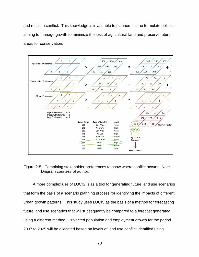
73
and result in conflict. This knowledge is invaluable to planners as the formulate policies
aiming to manage growth to minimize the loss of agricultural land and preserve future
areas for conservation.
Figure 2-5. Combining stakeholder preferences to show where conflict occurs. Note.
Diagram courtesy of author.
A more complex use of LUCIS is as a tool for generating future land use scenarios
that form the basis of a scenario planning process for identifying the impacts of different
urban growth patterns. This study uses LUCIS as the basis of a method for forecasting
future land use scenarios that will subsequently be compared to a forecast generated
using a different method. Projected population and employment growth for the period
2007 to 2025 will be allocated based on levels of land use conflict identified using

74
LUCIS for Lake County, Florida. A detailed description of the allocation method follows
in Chapter Three.
Summary
The relationship between land use and transportation in the United States is
longstanding and complex. While history has shown that innovations in transportation
technology have enabled increasing levels of mobility for most Americans, their desire
to live in low density suburban locations has simultaneously driven their need for greater
mobility. At the centre of the land use and transportation relationship is the automobile
and the high level of dependency most Americans have developed for it.
Public concerns about the negative social and environmental impacts of
transportation and the urban growth it has fostered have led to government policies
aimed at controlling and mitigating these effects. Research into the relationship
between land use and transportation has been largely driven by these concerns.
Despite a trend of increasingly focused research into understanding this relationship,
there still remains a considerable gap in the understanding of the relationship‟s
dynamics. A coordinated approach to planning land use and transportation may offer
the greatest opportunity for positive change yet a best approach to achieve coordination
eludes both practitioners and researchers.
Research into the relationship between land use and transportation helps guide
decision makers in formulating policies aimed at minimizing negative effects of urban
growth. The use of transportation and land use models plays an important role in
understanding potential impacts of future changes to both the transportation system and
urban growth patterns. The quantitative demands required of these models are
predominantly a consequence of federal policies that more closely monitor the

75
environmental impacts of transportation investments and their associated increases in
automobile use. As more emphasis has been placed on the quantification and
forecasting of potential future impacts, land use and transportation models have
become increasingly more sophisticated and complex, relying heavily on computer
simulations based on a large number of assumed variables. Based in mathematical
and economic theories, complex models often give the impression of being scientifically
superior to less complex or rule-based models. As a result, over time forecasts
generated using more complex methods have become the basis from which future long-
range plans are developed, rather than being used as an assessment of outcomes of
proposed plans. Instead of planning for a desired vision of the future, emphasis is
centered on planning for a future forecasted on assumptions about variables that cannot
be known.
Emphasis given in the urban planning process to complex models and their
resulting forecasts has come at the expense of simpler models that offer equally
possible forecasts of the future. The use of other methods of forecasting such as
scenario planning techniques offer an opportunity to capture broader macro-trends that
more statistically derived forecasts are unable to capture due to their narrower focus on
micro-level simulations. When supplemented with more sophisticated approaches to
forecasting future land use change, such as land use suitability analysis, simpler
methods such as scenario planning may offer better opportunities to successfully
coordinate long-range land use and transportation plans than the more complex
mathematically driven models in common practice today. That hypothesis is tested in
this study which compares two methods of forecasting future land use change. One

76
method incorporates scenario planning techniques and suitability analysis to create a
vision based on a set of broadly defined mutually supportive policy goals. The other
method is mathematically derived used a gravity model and is based on historical
development trends and prescriptive land use guidelines from existing policy. The
following chapter details the methodology used to carry out this comparison.

77
CHAPTER 3 STUDY AREA AND TIME FRAME
Study Area Selection
Florida has a history of rapid population growth. While the national population
growth rate for the USA in the twentieth century was between 10 and 20 percent, the
state of Florida experienced rates of between 20 and 80 percent (Smith, 2005, p. 2).
The distribution of Florida‟s population has shifted geographically over time, with rapid
increases in the state‟s central and southern regions. Although the southeastern and
southwestern regions of Florida have experienced the most rapid rate of growth in the
twentieth century, with decade averages of 77% and 61% respectively (Table 3-1), the
central region has contained the largest proportion of the state‟s population since the
1960s (Figure 3-1). This trend is projected to continue. The central region is expected
to grow the most in terms of absolute population between 2010 and 2035, with 45% of
new Floridians predicted to reside in the central region (Table 3-2).
Table 3-1. Florida‟s population growth rates by region – percentage change per decade, 1900 to 2000
Region Northern Central Southeastern Southwestern
Years Increase (%) Increase (%) Increase (%) Increase (%)
1900 to 1910 31.1 60.6 70.0 89.9 1910 to 1920 13.6 36.9 120.2 79.0 1920 to 1930 16.5 74.6 171.3 68.3 1930 to 1940 19.3 23.1 74.6 14.6 1940 to 1950 31.5 43.4 79.3 34.1 1950 to 1960 36.9 89.7 113.5 105.5 1960 to 1970 18.4 37.0 48.4 61.6 1970 to 1980 24.9 48.3 44.5 75.8 1980 to 1990 23.8 38.9 26.5 52.0 1990 to 2000 21.6 22.9 23.1 31.2
Average Increase 23.8 47.5 77.1 61.2
Note. Adapted from “Florida population growth: Past, present and future” by S.K. Smith, 2005, p. 23.

78
Figure 3-1. Florida‟s population distribution by region, 1900 to 2000. Adapted from
“Florida population growth: Past, present and future” by S.K. Smith, 2005, p. 22.

79
Table 3-2. Florida‟s projected population increase (per thousand people) by region, 2010 to 2035
Region 2010 2035 Increase
2010 to 2035 Total Growth 2010 to 2035
Central 7,620 11,735 4,115 45% Northern 3,833 5,820 1,988 22% Southeastern 5,823 7,398 1,574 17% Southwestern 1,987 3,436 1,449 16%
Note. Based on an average of medium and high projections from “Florida population studies bulletin 153 - Florida county population projections, 2008 – 2035” by University of Florida Bureau of Economic and Business Research, & University of Florida Population Program, 2009.
Within the central region Orange County is expected to grow by the largest
amount for the period 2010 to 2035, increasing by approximately 736,000 people and
accounting for almost 18% of total growth in the region (Figure 3-2). Figure 3-2 shows
adjacent counties, such as Osceola, Polk, Brevard and Lake, will also experience
substantial population increases.

80
Figure 3-2. Florida‟s central region, projected population growth from 2010 to 2035. Note. Based on an average of medium and high projections from “Florida population studies bulletin 153 - Florida county population projections, 2008 – 2035” by University of Florida Bureau of Economic and Business Research, & University of Florida Population Program, 2009.
A comparison of projected gross population densities for counties in the central
region provides insight into the effect population growth will have in specific locations in
this region. For example, although Figure 3-2 shows Orange County will have the
largest increase in absolute numbers of new residents between 2010 and 2035, its
gross population density will only increase by 64% (Table 3-3). Conversely, Osceola
County will have only approximately half the amount of growth as Orange County, and

81
Lake County approximately one-third, yet their respective increases in gross population
densities are 117% and 84%. The differences in densities are even more pronounced
when viewed for the period 2000 to 2035, with Lake County increasing by 163% and
Osceola County by 263% (Table 3-3). This is a result of both Lake and Osceola
Counties having relatively lower existing populations than neighboring Orange County
and explains how a relatively low amount of population growth can still have dramatic
effects in terms of changing population densities.
Table 3-3. Florida‟s central region, gross population densities and increases from 2010 to 2035.
Gross Density
(people per acre) Increase
(%) Increase
(%) Increase
(%)
County 2000 2010 2035 2000 to
2010 2010 to
2035 2000 to
2035
Sumter 0.15 0.25 0.68 90 139 353 Osceola 0.21 0.35 0.75 67 117 263 St. Lucie 0.54 1.21 1.71 125 42 218 Lake 0.33 0.47 0.86 43 84 163 Hernando 0.42 0.57 0.99 33 75 133 Marion 0.25 0.33 0.56 31 69 122 Indian River 0.36 0.47 0.78 29 66 115 Pasco 0.73 0.95 1.56 30 65 114 Orange 1.55 1.99 3.26 28 64 110 Citrus 0.30 0.38 0.59 25 56 95 Levy 0.05 0.06 0.09 24 57 94 Polk 0.41 0.50 0.78 24 54 90 Hillsborough 1.49 1.83 2.79 23 53 88 Brevard 0.73 0.88 1.26 19 43 71 Volusia 0.62 0.73 1.01 17 39 63 Okeechobee 0.07 0.08 0.11 14 33 52 Pinellas 5.30 5.43 5.95 2 10 12 Seminole 1.84 0.76 1.19 -59 58 -35
Note. Based on an average of medium and high projections from “Florida population studies bulletin 153 - Florida county population projections, 2008 – 2035” by University of Florida Bureau of Economic and Business Research, & University of Florida Population Program, 2009. Gross density was calculated as gross area (land area less open water) divided by projected population.
The significant increases in gross densities for Lake and Osceola Counties may be
a “spill-over” effect from the higher density Orange County where employment
opportunities may be greater yet housing opportunities less affordable to specific groups

82
of workers. Census Bureau data regarding travel patterns for journeys to work between
these counties support this theory. Table 3-4 shows the residence and work counties
for workers in Lake, Osceola and Orange Counties for 1990 and 2000. In particular it
shows the number of workers travelling to Orange County from its adjacent counties,
and from Lake and Osceola Counties to their adjacent counties. Although most workers
live and work in the same county, a large number of Lake and Osceola residents travel
to Orange County for work, with Lake County experiencing the greatest relative
increase of 135% between 1990 and 2000. In 2000 25% of workers in Lake County and
45% of workers in Osceola County traveled to Orange County to work.
Table 3-4. Residence and work counties for workers in Lake, Osceola and Orange Counties for 1990 and 2000
Residence County
Work County
1990 2000 Change 1990 to
2000
% Change 1990 to 2000
Orange Orange 317,493 376,709 59,216 19 Osceola Orange 19,495 34,085 14,590 75 Lake Orange 8,516 20,009 11,493 135 Seminole Orange 70,609 80,875 10,266 15 Polk Orange 5,496 11,823 6,327 115 Brevard Orange 2,953 6,122 3,169 107
Lake Lake 42,777 51,842 9,065 21 Lake Orange 8,516 20,009 11,493 135 Lake Seminole 1,261 2,979 1,718 136 Lake Volusia 1,406 1,536 130 9 Lake Sumter 510 1,214 704 138 Lake Osceola 457 1,110 653 143 Lake Marion 658 629 -29 -4
Osceola Osceola 29,323 38,416 9,093 31 Osceola Orange 19,495 34,085 14,590 75 Osceola Lake 66 1,628 1,562 2367 Osceola Polk 362 560 198 55 Osceola Brevard 364 330 -34 -9 Osceola Indian River 49 35 -14 -29 Osceola Okeechobee 5 24 19 380
Note. Adapted from “Journey to work and place of work - Census 2000 data - 2000 County to county worker flow files” by United States Census Bureau, 2008.

83
Further support for the theory that Orange County‟s growth is spilling over into
surrounding lower density counties can be found in housing data for 2000 and 2008
from the United States Census Bureau. Table 3-5 shows the median value of owner-
occupied houses for Lake, Osceola and Orange County. Median values for both 2000
and 2008 were highest in Orange County and lowest in Lake County, with rates of
increase similarly highest in Orange and lowest in Lake County. The median value of
homes in Osceola was 8% less than in Orange County in 2000 and by 2008 homes
were more affordable in Lake County where their median value was 23% less than
those in Orange County. Although housing affordability is only one potential factor
influencing people‟s decisions of where to reside in relation to their employment, should
this trend continue it may result in an increase in the number of Lake and Osceola
County residents traveling to Orange County to work in the future.
Table 3-5. Median values of owner-occupied houses in 2000 and 2008
County Median Value ($)
2000 Median Value ($)
2008
Orange 107,500 243,400 Osceola 99,300 207,500 Lake 100,600 187,800
Note. Adapted from “2008 American Community Survey1-Year Estimates” by United States Census Bureau, 2008, and from “Profile of Selected Housing Characteristics: 2000” by United States Census Bureau, 2000.
An increasing number of residents traveling into Orange County to work will have
important implications for long-range transportation planning in adjacent Lake and
Osceola Counties. In Florida long-range transportation plans (LRTPs) are prepared at a
regional scale by agencies known either as a metropolitan planning organization (MPO)
or transportation planning organization (TPO). These organizations are responsible for
the creation of 20-year transportation plans which are updated every five years that

84
include strategies consistent with local and state planning objectives for the
municipalities within their region (Florida Department of Transportation, 2009, p. 4-2).
Osceola and Orange Counties are within the same MPO boundary, Metroplan
Orlando, meaning the transportation needs for these counties are planned jointly under
the same LRTP. Transportation planning for the projected needs of Lake County
however is addressed by the Lake-Sumter MPO (LSMPO) under their own LRTP. How
well these two MPOs coordinate their long-range plans is particularly relevant to the
enhancement of public transportation in Lake County which seeks to increase the
proportion of choice riders, or those traveling to work. With one in four residents of
Lake County traveling to Orange County to work, the need to coordinate transit plans is
especially important if increased ridership is to be achieved.
A MPOs long-range transportation plan is statutorily required to be consistent with
the future land use element and policies of the comprehensive plans of the local
governments within its jurisdiction (FDOT, 2009a, p. 4-14). In the case of Lake County
and the LSMPO, its LRTP must be consistent with one county and fourteen municipal
comprehensive plans. This represents a large number of plans to be consistent with
considering the relatively low number of people the LSMPO serves, around 211,000 in
2000 (UFBEBR, 2009). Orange, Seminole and Osceola Counties which fall under
Metroplan Orlando‟s LRTP, on the other hand, had a population of around 1.4 million in
2000 but only 26 comprehensive plans with which to coordinate. Figure 3-3 shows
municipality, MPO and TPO boundaries for the central Florida region. Planning
consistently across many jurisdictional boundaries may be particularly challenging for
the LSMPO if the number of residents traveling to Orange County is isolated to just a

85
few local governments rather than being spread more evenly across the region. Local
governments with few potential choice riders may have less interest in creating future
land use plans that support a future transit plan aimed specifically at increasing this type
of ridership.
Figure 3-3. Municipality, MPO and TPO boundaries for Florida‟s central region. Note. Map courtesy of author.
Lake County was chosen as the area for this study for several reasons. Firstly the
county is situated in the most populous region of the state and is projected to receive

86
the largest number of new residents over the next 25 years. Secondly, Lake County‟s
adjacency to rapidly growing Orange County creates opportunities for population growth
to “spill over” into Lake County, creating challenges for the coordination of long-range
transportation plans both within Lake County and with Orange County. And thirdly,
Lake County has a relatively high number of local governments within its MPO region,
which may increase the potential for uncoordinated urban growth and reduce the ability
of the LSMPO to reach some of its long-range planning goals, particularly those
concerning public transportation. These factors highlight a long-range planning
situation in Lake County that could benefit from the use of scenario analysis in the
formulation and coordination of its land use and transportation plans.
Study Time Frame
The time frame for this study was the period 2007 to 2025. This was determined
according the time period for which the data used was relevant and for the planning
horizons covered by the policy documents used in the study. It was necessary to select
a point in time from which population and employment projections would be calculated
for the scenarios to be compared in the study. The year 2007 was chosen as the
beginning of the time period because it was the year for which the most current property
parcel data was available for Lake County.
The end-year of 2025 was chosen based on several factors. Firstly, of the two
methods of forecasting land use change that are compared in this study, one is that
which was adopted in the LSMPO‟s current LRTP which covers the period 2005 to
2025. Secondly, the transportation demand model (TDM) used in the study is that used
by FDOT in their state-wide modeling of transportation demand. The model can be run
for selected future years of which 2025 is one. Thirdly, at the commencement of this

87
study the most current comprehensive plan and therefore future land use map for Lake
County was also for the period 2005 to 2025. And lastly, projected population and
employment data for all of Florida‟s counties was available from the University of
Florida‟s Bureau of Economic and Business Research (BEBR) for several years
including 2025. Since two of the main policy documents guiding this study describe
plans up to the year 2025 and that a TDM specific to that year which uses data created
by one of the methods under investigation, 2025 was deemed most appropriate year to
end the study period.

88
CHAPTER 4 METHODOLOGY
Methodology Overview
This study uses land use and transportation modeling techniques to compare
three future urban growth scenarios for Lake County, FL in the year 2025. Two different
methods are used to allocate projected population and employment growth for the
period 2007 to 2025 to specific locations within Lake County. One growth scenario
uses the method adopted by the Lake-Sumter Metropolitan Planning Organization
(LSMPO) in the preparation of its 2025 Long Range Transportation Plan (LRTP). Two
alternative growth scenarios use a method that combines the use of the Land Use
Conflict Identification Strategy (LUCIS) and land use suitability analysis, and
concentrate urban growth at varying densities around future transit routes. This study
determines which of the three scenarios best reflects two long-range planning goals
Lake County seeks to achieve; specifically a more compact urban form, and increased
energy conservation by reducing single-occupancy vehicle (SOV) dependency and
increasing transit ridership. The findings of this study demonstrate which of the two
methods results in a future land use pattern that was most supportive of the specified
long range planning goals. By highlighting how different methods of forecasting future
land use effect the achievement of long-range planning goals, this study will alert state,
regional, and local government planning agencies of the benefits alternative methods
can have in improving the coordination of land use and transportation plans.
Figure 4-1 is a diagram explaining the methodology used in this study that will be
discussed in detail in the following sections of this chapter.

89
Figure 4-1. Diagram of study methodology.
90
Step One
The diagram of the study methodology shown in Figure 4-1 is a generalized
representation of the overall process and is divided into two halves. One half refers to
the creation of a scenario using the Florida land use allocation method (FLUAM) which
is the forecasting method adopted by the LSMPO in the creation of their 2025 LRTP.
The other half of the diagram refers to the creation of two scenarios using the LUCIS-
plus allocation method. LUCIS-plus (LUCIS-planning land use scenarios) is the name
tentatively given to a population and employment allocation method currently under
development in the Department of Urban and Regional Planning at the University of
Florida by Dr. Paul Zwick (P. Zwick, personal communication, March 19, 2010). The
methodology is further divided into three steps, of which this section discusses the first.
Florida Land Use Allocation Method Scenario Data
It should be noted that the FLUAM scenario was not created in this study. It is an
accompanying dataset to the CFRPM version 4.5 provided by the FDOT District 5 for
use in this study. The 2025 land use and socio-economic data for Lake County used
in the CFRPM was supplied to FDOT by the LSMPO (J. Banet, FDOT, personal
communication, February 9, 2010). Chapter Five of the Lake-Sumter 2025 LRTP
describes the methodology used to forecast future land use and socio-economic data
for their 2025 plan (Lake-Sumter Metropolitan Planning Organization, 2006, p. 5-1).
Datasets used in the forecast are included in Chapter 5 of the LRTP (pp. 5-2 - 5-3) and
are listed as follows:
University of Florida BEBR population projections – average of medium
and high projections for 2025

91
Vacant parcels from the year 2000;
The Future Land Use Element from the Lake County Adopted
Comprehensive Plan;
Traffic analysis zones used in the CFRPM;
Locations of master planned unit developments (PUDs) and developments
of regional impact (DRIs);
Environmentally sensitive land, such as the Green Swamp, Wekiva Basin,
and the Ocala National Forest;
Lakes and rivers; and
Other lands that are not able to be developed.
Land Use Conflict Identification Strategy Planning Land Use Scenarios Data
The LUCIS-plus scenarios were created using similar types of data as the FLUAM
scenario such as population and employment projections, parcel and traffic analysis
data, and environmental data. A comprehensive list of data used in the creation of the
LUCIS-plus scenarios is shown in Appendix C. A general list of data used is as follows:
Population and household estimates for 2007;
TAZ data for the years 2000 and 2012;
Average of medium and high population projections for 2025;
Employment projections for 2005, 2010 and 2025;
Parcel data for 2007;
Lakes and ponds;
Conservation areas;
LUCIS suitability and conflict rasters;

92
Visionary transit lines and stops for 2035; and
Projected school enrolment data for 2025.
The list shown in Appendix C shows the tabular and GIS data used, however other
types of information were also used in the construction of the LUCIS-plus scenarios,
such as policy guidelines. As these additional sources of information are used in the
methodology they will be discussed at that point in more detail.
Step Two
The second step of the methodology involves the allocation of projected
population and employment to specific locations across the study area. This is
achieved using different methods for the FLUAM scenario and the LUCIS-plus
scenarios. The datasets created for each of these scenarios are inputs to the third step
of the methodology which involves the modeling of transportation demand for each
scenario using the CFRPM. The CFRPM requires the datasets to contain a particular
set of attributes necessary to calculate travel demand in the model. An overview of
those attributes begins this section on Step Two and is followed by a more detailed
explanation of both FLUAM and LUCIS-plus and how they are used to create the three
scenarios compared in this study.
Transportation Analysis Zone Data – Overview
The CFRPM requires socio-economic data for each TAZ in the study area, often
referred to generally as TAZ data. The TAZ data are both a reflection of forecasted land
uses and the distribution of population and employment across those land uses. The
TAZ data for the CFRPM are further divided into two sub-sets. One dataset called
ZDATA1 is used to calculate trip productions and accounts for residential land uses,
their population and number of automobiles. The other dataset called ZDATA2 is used
93
to calculate trip attractions and accounts for employment land uses and the number of
employees in each location. The CFRPM requires each dataset, ZDATA1 and
ZDATA2, to be in a database-file, or .dbf format. Appendix D lists the attributes and their
descriptions for each dataset.
In this study, after population and employment have been allocated for each
scenario the data is tabulated so that a ZDATA1.dbf and a ZDATA2.dbf exists for each
of the three scenarios to be modeled with the CFRPM.
FLUAM – the Florida Land Use Allocation Method
FLUAM is the method used by the LSMPO for the creation of socio-economic data
used in the preparation of their 2025 LRTP, and thus is the method that was used for
the FLUAM scenario of this study, which uses the same dataset. Data processing
occurs using both GIS vector and tabular data, with final data compiled in a tabular
format. FLUAM is comprised of four general steps (LSMPO, 2006, p. 5-1):
1. Development of control totals;
2. Determination of developable lands;
3. Input of approved developments, manual adjustments, and overrides; and
4. Allocation of growth to traffic analysis zones.
Development of control totals
Tabular data are used to develop control totals for population, dwelling units and
employment totals for the county which are based on historical growth rates and an
average of medium and high projections from BEBR for 2025 (LSMPO, 2006, p. 5-2).
School enrollment forecasts also are included in the control totals as well as hotel/motel
dwelling units from approved developments (LSMPO, 2006, p. 5B-6).
94
Determination of developable lands
Developable lands are determined using parcel data in a GIS vector format for the
year 2000 as this is date of the last Census and therefore the most accurate population
data available. Using GIS processes the parcel data, which contains land use codes
used by the Florida Department of Revenue (FDOR), is queried to locate vacant parcels
and a GIS layer is created containing these parcels. This layer is combined with GIS
data for environmentally sensitive lands, lakes and rivers, and other undevelopable
land, which are subsequently selected and removed from the layer. PUDs and DRIs
are also removed as they are added in a later step of the process. TAZ and future land
use data are combined with the layer so that all vacant parcels can be summarized
according their future land use by TAZ number. A table is then created using the
attributes of this GIS layer and the total acreage of vacant developable land uses
available in each TAZ is summarized (LSMPO, 2006, p. 5-3). Figure 4-2 shows a
graphic representation of this part of the FLUAM process.
Input of approved developments, manual adjustments and overrides
For the development of factors used in the allocation process the study area is
delineated into ten planning areas that have similar development characteristics based
on the following (LSMPO, 2006, pp.. 5B-12-5B-13):
Existing land use;
Future land use;
Existing population and employment;
Location of cities;
Major roadway corridors;

95
Character of areas; and
Functional relationship of land uses.
Figure 4-2. Determination of developable lands in FLUAM
Source. “Lake-Sumter 2025 Long-Range Transportation Plan” by LSMPO, 2006, p. 5-4
Activity centers are then located for each planning area by calculating the amount
of employment and dwelling units per TAZ. Depending on their amount of employment
and dwelling units each TAZ is assigned a weight and these weights are then combined
for each planning area to determine where the centers of most activity are located
(LSMPO, 2006, p. 5B-13).
Densities and intensities of land uses are required by FLUAM to distribute
population and employment into the developable lands layer. These are calculated for
each planning area by comparing the existing built-out densities for each land use and
the maximum allowable densities contained in the Lake County Comprehensive Plan

96
(LSMPO, 2006, p. 5B-10). For example, an existing urban area that is fully developed,
or built-out, may have a residential density of four dwelling units per acre, whereas the
Comprehensive Plan indicates the maximum density allowed was five dwelling units per
acre. By dividing the built-out density by the maximum allowed density, a multiplier
factor can be calculated for guiding density in future locations of that land use. In this
example the density multiplier would be 0.8.
Densities are estimated for each TAZ based on their Comprehensive Plan
designation and multiplier factors applied to the unoccupied developable land. If for
example a TAZ has five acres of developable land for residential uses and an approved
density of four dwelling units per acre, then using a density multiplier of 0.8 the
maximum number of dwellings for the vacant developable land in this TAZ is eight (i.e. 5
x 4 x 0.8 = 8). Employment density factors are calculated in the same way (LSMPO,
2006, p. 5B-11). By calculating the maximum allowable dwelling units and employment
that vacant developable land can accommodate, the allowable growth for each TAZ is
calculated. The maximum development each TAZ can accommodate is then calculated
by adding the allowable growth to the existing development which is then used to
determine if the allocated growth is physically possible within each TAZ. If the growth is
not possible the model re-allocates it to other TAZs (LSMPO, 2006, p. 5B-12).
Allocation of growth to TAZs
The allocation of dwelling units and employment is based on the control totals and
the maximum allowable development for each TAZ, and is performed using a
spreadsheet. Allocations for PUDs and DRIs are input manually into the spreadsheet
as the population and employment numbers are known for these areas, based on the
information included in their development approvals. The remainder of the population
97
and employment totals is allocated using a gravity model which assigns each TAZ an
attractiveness factor (LSMPO, 2006, p. 5B-14). A gravity model is based on the
concept that activity centers within a study area exert an influence on surrounding
locations based on the activity centre size and number of available activities. An
attractiveness factor for each TAZ is calculated using the size of the nearest activity
centre divided by the square of the distance of the TAZ to the activity centre. TAZs with
higher attractiveness factors are considered to develop faster than those with lower
factors (LSMPO, 2006, p. 5-4). The attractiveness factor is used in combination with
how close each TAZ is to other TAZs and the planning area‟s centre. Growth is then
allocated first to, and filling, TAZs closest to the planning area centre in a way that
simulates compact urban development (LSMPO, 2006, p. 5B-14).
School enrollment is entered manually into the TAZs where each school is located.
The school enrollment from the prior LRTP is reviewed and where determined, due to
forecasted increased enrollments in specific locations, additional school locations are
assigned. Approved developments that include new schools are added to the
appropriate TAZ and the approved number of students is allocated (LSMPO, 2006, p.
5B-15). Hotel/motel units are also allocated manually and are based on the number
and location of units in 2000. Units created as part of approved developments are
added, and likely locations of new units is determined through consultation with County
and municipal staff (LSMPO, 2006, p. 5B-15). Finally, all of the socio-economic data is
tabulated into two .dbf files, ZDATA1 and ZDATA2 for inputting into the CFRPM.
LUCIS-plus – The LUCIS Planning Land Use Scenarios Method
LUCIS-plus is a GIS raster-based method for allocating regional population and
employment growth. It is currently being developed by Dr. Paul Zwick at the University

98
of Florida as a scenario planning tool for use in a wide range of planning fields,
including environmental and conservation planning, transportation planning and hazard
mitigation planning (P. Zwick, personal communications, 2010). The method employs
the use of the ESRI software ArcMap and its associated ModelBuilder application. A
suite of models are created that produce rasters capable of representing different future
land use scenarios. Research and development of LUCIS-plus has also included the
creation of several complimentary tools that work in conjunction with the suite of models
that enable planners to input scenario parameters via simple GUIs (graphical user
interfaces) containing drop-down menus for the selection of desired variables (A. Arafat,
personal communication, March 15, 2010). Additionally, programs using Python and
VB (Visual Basic) scripts have been developed as part of the LUCIS-plus research so
that the raster data can be summarized into a manageable tabular format for easier
analysis and integration into other modeling frameworks, such as transportation
demand and hazard simulation models.
This study uses LUCIS-plus as a method for creating two scenarios however it
does not use the complimentary tools or additional programs noted above. Instead data
inputs and variable parameters are entered manually into models, allocation fields
within the rasters are calculated manually, and output rasters are also manually
summarized for the creation of ZDATA tables.
There are differences between the FLUAM and the LUCIS-plus methods however
it is important to note one major difference between them before describing the study
methodology further. The scale at which growth is allocated in both methods is vastly
different. FLUAM allocates growth at the TAZ level, meaning future population and

99
employment are distributed across zones that vary in size from approximately 20 to
40,000 acres. The average size of a TAZ is approximately 2,800 acres. LUCIS-plus
allocates growth at a much smaller scale as it uses rasters containing cells that are 31
meters square, approximately one-quarter acre in size, to reflect the average-sized
residential building lot. In the LUCIS-plus scenarios growth is allocated to raster cells
and then aggregated to a TAZ level at the end of the allocation process.
It is possible to aggregate data from the smaller scale LUCIS-plus scenarios up to
the larger scale TAZ level so that it can be compared with data from the FLUAM
scenario. However, it is not possible to disaggregate the larger scale FLUAM data
down to a smaller scale for comparison with the LUCIS-plus data. Smaller scale data
used in the creation of the FLUAM scenario, such as the specific parcel and land use
data, was not available to this study. In the absence of such information any attempt to
disaggregate the larger scale data would require a large measure of estimation that
would nullify any meaningful comparison between the FLUAM and LUCIS-plus
scenarios. The comparison of scenarios in this study is therefore undertaken at the
larger TAZ scale rather than the smaller quarter-acre scale.
Following is a general list of steps used to create the two LUCIS-plus scenarios for
this study; each will subsequently be described in more detail. Not all of the steps listed
are strictly speaking a part of the LUCIS-plus method. For example, the second, third
and fifth steps involve the calculation of gross land use densities, control totals for
population and employment growth, and specific growth patterns such as land use
intensities. These are variables needed for input into models used in LUCIS-plus, but
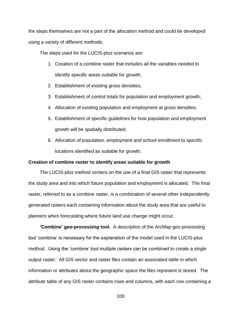
100
the steps themselves are not a part of the allocation method and could be developed
using a variety of different methods.
The steps used for the LUCIS-plus scenarios are:
1. Creation of a combine raster that includes all the variables needed to
identify specific areas suitable for growth;
2. Establishment of existing gross densities;
3. Establishment of control totals for population and employment growth;
4. Allocation of existing population and employment at gross densities;
5. Establishment of specific guidelines for how population and employment
growth will be spatially distributed;
6. Allocation of population, employment and school enrollment to specific
locations identified as suitable for growth.
Creation of combine raster to identify areas suitable for growth
The LUCIS-plus method centers on the use of a final GIS raster that represents
the study area and into which future population and employment is allocated. The final
raster, referred to as a combine raster, is a combination of several other independently
generated rasters each containing information about the study area that are useful to
planners when forecasting where future land use change might occur.
‘Combine’ geo-processing tool. A description of the ArcMap geo-processing
tool „combine‟ is necessary for the explanation of the model used in the LUCIS-plus
method. Using the „combine‟ tool multiple rasters can be combined to create a single
output raster. All GIS vector and raster files contain an associated table in which
information or attributes about the geographic space the files represent is stored. The
attribute table of any GIS raster contains rows and columns, with each row containing a
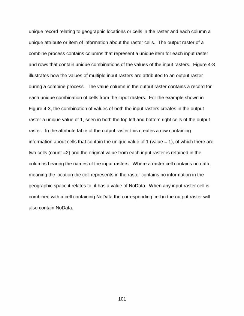
101
unique record relating to geographic locations or cells in the raster and each column a
unique attribute or item of information about the raster cells. The output raster of a
combine process contains columns that represent a unique item for each input raster
and rows that contain unique combinations of the values of the input rasters. Figure 4-3
illustrates how the values of multiple input rasters are attributed to an output raster
during a combine process. The value column in the output raster contains a record for
each unique combination of cells from the input rasters. For the example shown in
Figure 4-3, the combination of values of both the input rasters creates in the output
raster a unique value of 1, seen in both the top left and bottom right cells of the output
raster. In the attribute table of the output raster this creates a row containing
information about cells that contain the unique value of 1 (value = 1), of which there are
two cells (count =2) and the original value from each input raster is retained in the
columns bearing the names of the input rasters. Where a raster cell contains no data,
meaning the location the cell represents in the raster contains no information in the
geographic space it relates to, it has a value of NoData. When any input raster cell is
combined with a cell containing NoData the corresponding cell in the output raster will
also contain NoData.

102
Figure 4-3. The „combine‟ process.
Source. “ArcGIS Desktop 9.3 Help – Combine” by ESRI, 2010.
Allocation buffers. In this study five combine rasters are created for each
LUCIS-plus scenario. In total 10 combine rasters are created; five for a low density
LUCIS-plus scenario and five for a high density LUCIS-plus scenario. For each
scenario the five combine rasters represents an allocation of population and
employment into a specific zone or allocation buffer. The combine rasters contain 31
meter by 31 meter cells, creating a high spatial resolution and increasing file size as the
extent of each allocation buffer increases. To increase computational speed of the
models and the allocation process it was determined that a separate combine raster for
each allocation buffer would be necessary. Data from the five combine rasters are
collated once all allocations have been made for each scenario to create the ZDATA1
and ZDATA2 .dbf files necessary for step three of the methodology.
The five allocation buffers are illustrated in Appendices E through Hand include a
description and rationale of the buffer distances. The location of transit stops used in
the creation of the buffer zones are those contained in a GIS vector file created by the

103
ECFRPC of visionary future transit routes and stations used in modeling future growth
for their 2060 Strategic Regional Policy Plan (P. Laurien, personal communication,
January 20, 2010).
Combine raster model. Each combine raster is created using a similar LUCIS-
plus model. Model inputs and outputs are the same for each of the combine rasters,
with the exception of the buffer raster which determines the spatial extent of the
allocation and the inclusion of DRI (developments of regional impact) rasters in buffers
4 and 5. Figure 4-4 shows the model of the combine raster for the allocation of buffer 1
and will serve as an example for explaining the functioning of all the combine raster
models. For ease of explanation the illustration of the model highlights three phases
that will be described separately. When the model is run the processing occurs in the
order the phases follow.
Combine model – phase one. Data inputs to the first phase of the model include
a raster of the extent of buffer 1 and a raster of the opportunities for mixed use
development. The buffer 1 raster was created by converting a vector shapefile of the
area to a raster and then reclassifying the cells so that only cells representing the
location of buffer 1 contain a value and all other cells are assigned a NoData value.
When this raster is combined with all other input rasters in the combine model all cells
that overlap the NoData cells will also be assigned a NoData value, thereby masking
those cells out of the output raster. This process is referred to as creating a mask. In
the combine models of this study the buffer rasters act as masks for delineating where
specific configurations of urban growth will occur.
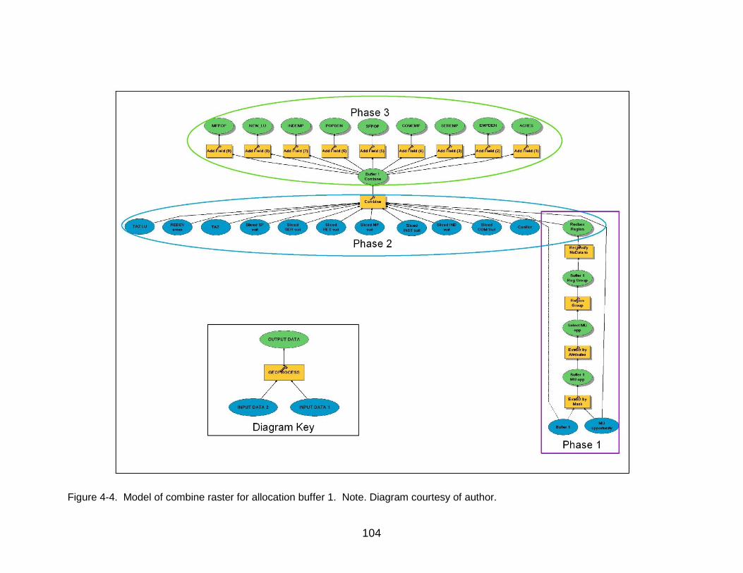
104
Figure 4-4. Model of combine raster for allocation buffer 1. Note. Diagram courtesy of author.
105
The raster representing the opportunities for mixed use development was created
in a separate model that combines individual preference rasters for each of the following
land uses; commercial, institutional, multi-family, retail and service which represent the
mix of uses that are desirable in TOD areas. Each cell in the mixed use opportunities
raster contains a 5-digit value that represents the level of conflict or opportunity that
exists between the different land uses in that cells location. For example a cell with a
value of 33333 represents a good opportunity for mixed use as all of the land uses are
highly preferred in that location, and a cell with a 11111 value has few mixed use
opportunities.
Using an extraction tool the values from the mixed use opportunities raster are
extracted based on their location within buffer 1. Cells with a high opportunity for mixed
use were extracted next. Only cells that had a high preference (3) for multi-family
combined with a medium (2) or high (3) preference for any of the other land uses were
extracted. The suitability of areas for mixed use development is also influenced by the
size or acreage of land under consideration. Areas of less than an acre are likely to be
less desirable for this type of development. Therefore it is necessary to locate cells of
high mixed use opportunity that are clustered into groups of raster cells of four or more;
as each raster cell is approximately one-quarter acre. This is performed in the model
using the „region group‟ process which is illustrated in Figure 4-5.

106
Figure 4-5. The region group process
Source. “ArcGIS Desktop 9.3 Help – Region Group” by ESRI, 2010.
During the region group process the value of the output raster cells represents a
unique value that corresponds to its relationship with its neighboring cells. The process
moves through the raster starting in the cell in the top left corner moving to the right and
down through subsequent rows. The attribute table of the output raster contains a
column listing the count of cells with the same value. Using Figure 4-5 as an example,
if the cell sizes had an area of one-quarter acre then none of the cells are grouped in a
one acre configuration, meaning in the attribute table none had a count of 4 or greater.
In this example the highest count is 3, representing an area of only three-quarters of an
acre.
At this point in phase one the output raster (Buffer 1 Reg Group) contains all the
cells in buffer 1 that have a high opportunity for mixed use development. The cells also
have a value that represents their relationship to neighboring cells so that groups of a
certain size can be located. The final stage of phase one involves reclassifying the cells
with a value of NoData to zero so that all data is retained during the subsequent
combine process of the model.

107
Combine model – phase two. The second phase of the model uses the combine
process described earlier. Fourteen rasters form the data inputs to the process which
represent the different attributes necessary for defining suitable locations for future
urban growth. Seven of the fourteen rasters represent different land use suitabilities
determined using the LUCIS process described in the literature review. The original
suitability rasters were created by Dr. Paul Zwick of the University of Florida as part of a
study for the ECFRPC in 2008-2009 concerning future land use change in the central
Florida region. The seven rasters represent the suitability for the following land uses:
single family residential, multi-family residential, commercial, service, retail, institutional,
industrial.
Each suitability raster contains values ranging from 1 to 9, with 9 representing the
highest suitability and 1 the lowest suitability. In the attribute table of each suitability
raster therefore only 9 records or values exists, and each value has a count
representing the number of cells with that unique value. In this study cells are selected
based on their suitability using a tool that queries the attribute table to select cells with
particular values, for example select all cells with a value equal to 9, or select all cells
with a value of less than 7 but greater than 4. It is not possible therefore to select a
fewer number of cells than there is in total for that value. For example, if only 90 cells
were needed with a value of 9 but that row in the attribute table (with a value of 9)
contained a total of 200 cells it would not be possible to select fewer than 200 using this
selection method. Therefore it is necessary to reclassify the data so that there is a
greater range of values on which to base selections. A slice tool is used to reclassify

108
the data into smaller slices, or more values in the attribute table. The seven suitability
rasters were reclassified into 1,000 slices of equal area.
A raster representing the level of conflict between the three major land use groups
of agriculture, conservation and urban is included as an input. This raster was also
created by Dr. Zwick for the ECFRPC study mentioned earlier. The cell values of this
raster represent the preference for each of the three land use groups, with a value of
333 corresponding to an area that is equally preferred by all uses, and a value of 111
representing an area that has a low preference for all three.
A raster of land uses is included as an input so that existing population and
employment can allocated according to their land use. The land use values correspond
to the generalized TAZ land use categories listed in Appendix I. A raster of the TAZs is
also included so that each cell can be summarized in the final stage of the allocation
process according to its TAZ. A buffer raster is included in the combine process that
acts like a mask so that only cells located in that buffer are included in the output
combine raster. The mixed use opportunities raster described in phase one is also
included as is the region group raster that was a result of phase one.
The remaining input raster is one that represents areas that have a potential for
redevelopment. This was created by querying the vector parcel data to locate areas
that met certain criteria and then exporting the file to a raster format. The selection
criteria for redevelopment parcels are as follows:
Cells within half-mile buffer of future transit stations;

109
Parcels with a „just value‟ that is below the average „just value‟ for
properties of the same land use - „just value‟ is the price a property may
sell for in an open market – it is synonymous with „market value‟;
Parcels with buildings that will be more than 50 years old in 2025, i.e. were
built prior to 1975; and
Exclude parcels with the following uses – churches, orphanages, hospitals,
schools, sanitariums, homes for the aged, and cemeteries.
Combine model – phase three. The third phase of the LUCIS-plus model
involves the adding of necessary fields for the allocation process. These fields are as
follows:
MFPOP – for multi-family population
SFPOP – for single family population
COMEMP – for commercial employment
SEREMP – for service employment
INDEMP - for industrial employment
EMPDEN – for employment density
POPDEN – for population density
NEW_LU – for new land use code
ACRES – for total acres
The LUCIS-plus model is then run five times for each scenario, each time using one of
the five buffers as a mask.

110
Establishment of existing gross densities
To identify areas suitable for future growth the size and distribution of existing
population and employment must first be determined. GIS vector-format parcel data
from the year 2007 was the most current land use data available during the study and
forms the basis for establishing the extent and land use distributions of the urban form
in the study area. The parcel data contains a land use code used by the FDOR, which
identifies individual land uses across a range 99 different uses. This study compares
only five different land use categories; single family residential, multi-family residential,
commercial, service, and industrial uses. The FDOR codes are aggregated to reflect
the five generalized land use categories of this study. Appendix I lists the FDOR codes
aggregated to reflect TAZ land use codes. A table containing the TAZ land use codes is
joined to the GIS parcel layer and the TAZ land use codes are copied over to a new
field within the parcel layer called TAZ_LU.
Land that is not available for development is then removed from the parcel layer
using the GIS „erase‟ geo-processing tools which removes areas from the parcel layer
that overlap with the „erase‟ layer. Conservation areas and lakes and ponds are
removed from the parcel layer in this way. Roads, rights-of-way and other
undevelopable land uses such as undefined and centrally assessed parcels are
removed by selecting them from within the parcel layer and deleting their records from
the layer‟s associated attribute table. The total number of acres within each of the TAZ
land use categories is then calculated by summing the area of the individual parcels
within each category. Table 4-1 shows the total acreage in the study area by TAZ land
use categories. The total number of acres for each land use is the denominator in the

111
calculation of gross density: Total population or employment in land use X ÷ Total
acreage of land use X.
Table 4-1. Total acreage by TAZ land use categories.
TAZ Land Use Category Total Acres
Single family residential 67,734 Multi-family residential 1,482 Mobile homes residential 29,312 Commercial 3,256 Service 37,276 Industrial 161,044 Vacant residential 69,213 Vacant commercial 5,859 Vacant industrial 1,325 Vacant 29,969
Total acres 406 ,470
The numerator in the gross density calculation is the total population or
employment in a particular land use. Population values are calculated by averaging
data from the Census Bureau and available TAZ data. Census Bureau estimates of
population and dwelling units by type of residence for the year 2007 are summarized
according to their residential TAZ land use code; single family, multi-family or mobile
home. These population totals are then divided by the total number of acres in each
land use category to determine a gross density. Table 4-2 lists Census Bureau
population estimates and the gross density for each residential TAZ land use.
Table 4-2. Census Bureau estimates for 2007 for Lake County population by residential TAZ land use categories
TAZ Land Use Category Population Total Acres Gross Density
Single family residential 171,335 67,734 2.53 Multi-family residential 40,360 1,482 27.24 Mobile homes residential 73,272 29,312 2.51
Total population 284,967 98,528 2.89
Source. Adapted from “Selected housing characteristics: 2005-2007, Lake County Florida” by United States Census Bureau, 2007.

112
TAZ data is also used to supplement the Census Bureau population estimates.
TAZ data for the years 2000, 2012 and 2025 is provided with the CFRPM and the
datasets for 2000 and 2012 are compared to calculate an average annual increase in
population and employment totals over that period. The average annual increase is
then applied to the 2000 TAZ data to project totals forward to the year 2007. Population
and employment totals are summarized by TAZ land use category and gross densities
calculated. Table 4-3 lists the population estimates and gross densities; employment
estimates are listed in a subsequent table.
Table 4-3. TAZ estimates for 2007 for Lake County population by residential TAZ land use categories
TAZ Land Use Category Population Total Acres Gross Density
Single family residential 163,994 67,734 2.42 Multi-family residential 38,747 1,482 26.15 Mobile homes residential 70,127 29,312 2.39
Total population 284,967 98,528 2.77
Gross density estimates from both the Census and TAZ data are averaged to
establish the gross residential densities that will be used to distribute existing residential
population across the study area. Table 4-4 lists the existing gross residential densities
for the study area.
Table 4-4. Existing gross residential densities for study area
TAZ Land Use Category Census TAZ Existing
Gross Densities
Single family residential 2.53 2.42 2.48 Multi-family residential 27.24 26.15 26.69 Mobile homes residential 2.51 2.39 2.45
Gross density 2.89 2.77 2.83
Employment gross densities are calculated in a similar way, by averaging two
sources of estimates. Employment projections for the years 2005, 2010 and 2025
created by the ECFRPC for a 2008-2009 study of land use modeling techniques are
used to establish employment estimates for the year 2007. The 2007 estimate was

113
based on the average annual increase in employment between the 2005 and 2010
estimates. The ECFRPC used the REMI Policy Insight model, an econometric input-
output model, to project employment across 23 categories. These employment
categories are listed in Appendix J according to their TAZ land use category;
commercial, service or industrial uses. Table 4-5 lists the gross employment densities
using the ECFRPC employment projections.
Table 4-5. ECFRPC estimates for 2007 for Lake County employment by TAZ land use categories
TAZ Land Use Category Employment Total Acres Gross Density
Commercial 19,657 3,256 6.04 Service 75,681 37,276 2.03 Industrial 23,805 161,044 0.15
Total employment 119,143 201,576 0.59
Gross employment densities are calculated using the 2007 TAZ data and are
listed in Table 4-6.
Table 4-6. TAZ estimates for 2007 for Lake County employment by TAZ land use categories
TAZ Land Use Category Employment Total Acres Gross Density
Commercial 28,286 3,256 8.69 Service 62,069 37,276 1.67 Industrial 22,211 161,044 0.14
Total employment 112,566 201,576 0.56
Gross density estimates from both the ECFRPC and TAZ data are averaged to
establish the gross employment densities that will be used to distribute existing
employment across the study area. Table 4-7 lists the existing gross employment
densities for the study area.

114
Table 4-7. Existing gross employment densities for study area
TAZ Land Use Category ECFRPC TAZ Existing
Gross Densities
Commercial 6.04 8.69 7.36 Service 2.03 1.67 1.85 Industrial 0.15 0.14 0.14
Gross density 2.89 2.77 0.78
Establishment of control totals for growth
To establish the amount of growth to be allocated into the future scenarios,
estimates of 2007 population and employment are deducted from forecasts for 2025.
Table 4-8 lists the estimates and forecasts used and their averages that result in the
control totals used for this study.
Table 4-8. Population and employment control totals
Population Projections / Estimates Total Average Control Total
2025 Population – BEBR (med-high) 449,050 2025 Population – TAZ 463,500
2025 Population – Average 456,275 2007 Population – Census Bureau 288,580 2007 Population – TAZ 272,860
277,224
Total Population Growth 2007 to 2025 179,051
Employment Projections / Estimates Total Average Control Total
2025 Employment – ECFRPC 173,138 2025 Employment – TAZ 185,580
179,359 2007 Employment – ECFRPC 119,143 2007 Employment – TAZ 112,566 115,855
Total Employment Growth 2007 to 2025 63,504
Allocation of existing population and employment using gross densities
Using the attribute table of the combine raster for each of the buffers, cells are
selected based on their existing TAZ land use category. Once cells are selected the
field calculator tool is used to create a new value for the population or employment field

115
by multiplying the count of cells by the appropriate gross density. The following script
describes the calculation for the allocation of existing single family uses:
[COUNT] * (2.48/4.211) - where [COUNT] represents the number of cells with SF
use, 2.48 the SF gross density per acre and 4.211 the value by which the per acre
density must be divided to reflect the 31 by 31 meter cell size.
All cells with a TAZ land use of SF, MF, COM, SER and IND are selected and
population or employment is allocated to them using their existing gross density. The
NEW_LU field is also calculated to show a new land use code for each cell that reflects
the TAZ land uses. This is done so that the data can be summarized at the end of the
allocation process and also to show where which cells may have changed land uses.
Table 4-9 shows the NEW_LU codes.
Table 4-9. NEW_LU codes
Land Use Category
NEW_LU
Land Use Category
NEW_LU
Single family SF 1 Vac. Commercial VACCOM 8 Mobile home MOB 2 Vac. Residential VACRES 10 Multi-family MF 3 Agriculture AG 11 Industrial IND 4 Conservation CON 12 Commercial COM 5 Ag Preservation AGPR 13 Service SER 6 Mixed Use MU 14 Vac. Industrial VACIND 7 Vacant VAC 15
The attribute table of each of the five combine rasters is summarized so that the
total number of population, employment and acres can be tabulated.
Establishment of guidelines for distribution of growth
TOD guidelines. The two LUCIS-plus scenarios are examples of an urban growth
pattern that is compacted within existing transportation corridors and clustered near
future transit stations and routes to enhance the achievement of long-range
transportation goals. The low scenario allocates at a lower density and the high at a

116
higher density. Draft guidelines created by the FDOT for the design of TODs are used
to determine the appropriate mix of land uses, densities and intensities of development
within a one-quarter mile distance of transit stations. A range of development standards
are presented in the guidelines that reflects a variety of different urban contexts that,
depending on the type of planned future transit such as light rail or rapid bus, would be
most appropriate considering the existing and future land uses of the area (FDOT,
2009b, p. 2). According to Lake County‟s Transit Development Plan (TDP) for 2009 to
2020, the future transit system planned is one that enhances existing fixed route bus
transit, and incorporates new bus rapid transit and commuter rail routes. Appendix K
shows the planned transit system and a description of the modes and routes it includes.
Based on the type of transit in the TDP and Lake County‟s existing low density urban
development, the TOD standard chosen to guide this study is one described in the
FDOT design guidelines as T3. Appendix L shows the T3 standards.
4-6 shows an Excel spreadsheet used to calculate the densities for mixed use
development within TOD areas for the low LUCIS-plus scenario. This scenario uses the
low value in the ranges suggested by FDOT for TOD population, employment and
dwelling unit densities.

117
Figure 4-6. Calculation of mixed use densities for the low LUCIS-plus scenario.
Figure 4-7 shows an Excel spreadsheet used to calculate the mixed use densities
for the high LUCIS-plus scenario. This scenario uses the median of the medium and
high values in the ranges suggested by FDOT for densities in TODs.

118
Figure 4-7. Calculation of mixed use densities for the high LUCIS-plus scenario.
Establishing the amount of growth to be allocated into each buffer was performed
using an Excel spreadsheet that calculated the amount of growth in population and
employment for the period 2007 to 2025. Growth is compacted in both the LUCIS-plus
scenarios to within a three mile distance of existing and future transit routes. Based on
the existing proportions of single, multi family and mobile home populations within that
distance, adjustments are made in both scenarios to increase proportions thereby
compacting growth. In 2007 forty percent of the total population lived within a three mile
distance to transit and sixty percent outside of that distance. Sixty percent of the total
2007 population was in single family residential, fourteen percent in multi-family, and
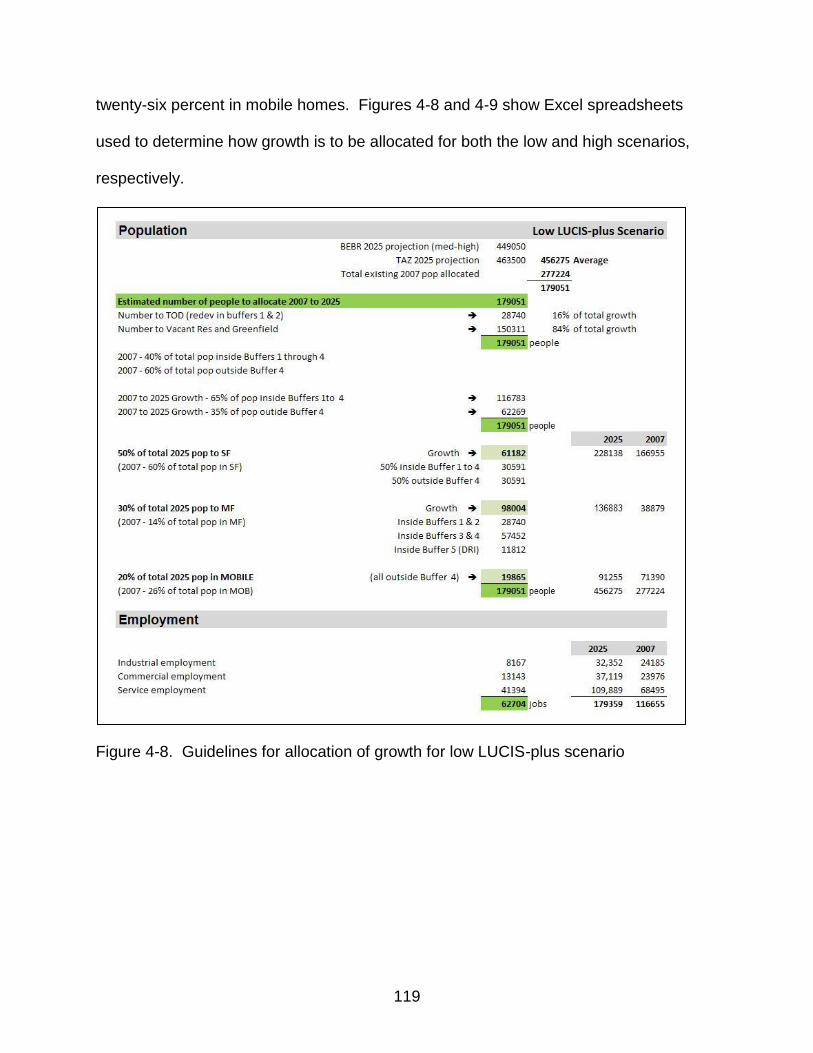
119
twenty-six percent in mobile homes. Figures 4-8 and 4-9 show Excel spreadsheets
used to determine how growth is to be allocated for both the low and high scenarios,
respectively.
Figure 4-8. Guidelines for allocation of growth for low LUCIS-plus scenario

120
Figure 4-9. Guidelines for allocation of growth for high LUCIS-plus scenario
Allocation of growth to suitable areas based on established guidelines
Order of allocations. In both LUCIS-plus scenarios growth is allocated in order
by buffer, beginning with buffers 1 and 2 which represent TOD areas, followed by buffer
3 which represents commercial corridors, then buffer 4 which includes remaining areas
within a three mile distance of transit, and finally buffer 5 which is the remainder of the
study area.
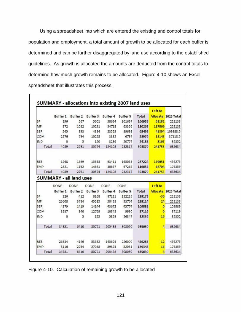
121
Using a spreadsheet into which are entered the existing and control totals for
population and employment, a total amount of growth to be allocated for each buffer is
determined and can be further disaggregated by land use according to the established
guidelines. As growth is allocated the amounts are deducted from the control totals to
determine how much growth remains to be allocated. Figure 4-10 shows an Excel
spreadsheet that illustrates this process.
Figure 4-10. Calculation of remaining growth to be allocated
122
For example, if the total amount of population growth for TOD areas (buffers 1
and 2) is 28,740 then beginning in buffer 1, a selection of the most suitable locations
can be made, and based on that area the amount of population that can be allocated
can be determined by dividing that area by the population or employment density. Thus
if 1,000 suitable cells are located in buffer 1 for multi-family population (i.e. 237.43
acres) then using the TOD density for multi-family (54.59 people/acre) a total of 12,963
people can be allocated in buffer 1. The remaining 15,777 people (28,740 less 12,963)
need to be allocated in buffer 2. A separate spreadsheet is used for each buffer‟s
allocations so that a running total is kept to guide what remains to be allocated. Once
all growth has been allocated in the buffer, the attribute table of the combine raster for
that buffer is summarized and the new population and employment totals are inserted
into the spreadsheet of control totals (Figure 4-10) to determine what remains to be
allocated in subsequent buffers.
Selection of suitable areas and allocation of growth. The selection of suitable
areas for allocating growth is steered firstly by the established guidelines and secondly
by land use suitability analysis. The allocation of growth to buffer 1 will be described in
detail as an example of how this process was undertaken for all of the buffers, and then
an overview of the selection process for the remaining buffers is provided Appendix M.
Example - allocation to buffer 1. Using the control totals the amount of
population and employment growth to be allocated is determined. As buffers 1 and 2
are TOD areas all population and employment growth is first to be allocated into
suitable locations for mixed use redevelopment and then into vacant land uses
(VACRES, VACCOM, VACINST or VAC). In this analysis all mixed use development
123
will incorporate both residential and commercial/service components. The residential
component is multi-family population and the employment component is divided
between commercial and service according to their relative proportion of total
employment growth. Twenty-five percent of all non-industrial employment growth is
forecasted to be commercial and seventy-five percent service, so in mixed use areas
the employment growth is distributed according to those percentages.
In the attribute table of the buffer 1 combine raster, a selection by attribute is
performed to firstly locate cells within redevelopment areas (RCLREDVBF1_2 > 0).
From this selection, cells that are grouped in areas of one acre or more (four or more
cells) are located (RREGIONBUFF1 >= 4). From this selection, cells that have a
medium to high mixed use opportunity are selected (RCINMFRSCONF = 33333 OR
RCINMFRSONF = 23333 OR ….RCINMFRSCONF = 22223). For the selected cells the
field calculator tool is used to allocate population and employment at the mixed use
densities into the appropriate fields (MFPOP, COMPOP and SERPOP). A NEW_LU
code of 14 (MU) is also calculated. The count of cells in the selection is entered into the
buffer 1 working spreadsheet and the remaining number of cells to be allocated is
calculated.
The remaining growth for buffer 1 is to be allocated into vacant land uses (VAC,
VACRES, VACCOM and VACINST). This selection starts by selecting all cells that
have not already been allocated in the previous step (NEW_LU = 0), then selecting all
cells that have vacant uses (TAZ_LU = VAC OR TAZ_LU = VACRES…). From this
selection all cells that have a medium to high mixed use opportunity are selected,
followed by those grouped in areas one acre or larger. Using the field calculator,

124
population and employment is allocated to the appropriate fields and an NEW_LU code
of 14 is given. The count of cells in the selection is entered into the spreadsheet and if
any growth remains unallocated it is carried over to buffer 2. Finally the attribute table
of the combine raster is summarized and the new population and employment totals are
added to the control totals spreadsheet (Figure 4-10) so that an accurate count of
remaining growth can be determined.
Allocation to remaining buffers. Allocation of growth to the remaining buffers
continues in a similar way. Opportunities for mixed use redevelopment exist in buffers
1, 2 and 3 and are selected first in those buffers, followed by vacant land uses based on
their level of land use conflict, followed by the suitability for individual land uses. Mixed
use opportunities do not exist in buffers 4 and 5 so selection in those buffers begins with
allocation into DRIs and the remainder according to land use conflict and land use
suitability. The method of allocation is the same for both the low and high LUCIS-plus
scenarios with the only difference between them being their level of compactness (as
determined by their allocation guidelines) and their mixed use densities. Appendix M
lists the general steps and criteria used for allocation in all buffers.
Creation of ZDATA tables. Once all growth has been allocated, summaries of all
the combine raster attribute tables are collated into one spreadsheet. The data is then
summarized according to TAZ number and the data separated according to the required
attributes of the ZDATA1 and ZDATA2 .dbf files. Appendix D lists those attributes and
highlights in bold type the attributes that are derived from the LUCIS-plus method. The
dwelling units totals (SFDU and MFDU) are calculated by dividing the SFPOP and
MFPOP by the average household size of 2.48 people. With the exception of school

125
enrolment, the remaining fields are carried over from the 2025 TAZ data that
accompanies the CFRPM. School enrolment is calculated outside of the LUCIS-plus
method and is done using a combination of GIS and spreadsheet functions.
Allocation of school enrolment. School enrolment is calculated and allocated
following several steps. Using a GIS vector file of the school area zones, the 2025
population (as allocated in each LUCIS-plus scenario) is summarized. Then using data
from the Census Bureau 2007 household estimates, the percentage of school aged
children is determined according to school type (elementary, middle and high school).
These percentages are used to determine the number of school aged children in each
school area zone according to school type. Figure 4-11 shows a spreadsheet used to
calculate school enrolment for 2025 for the low LUCIS-plus scenario. A similar
calculation is done for the high LUCIS-plus scenario. TAZs where the individual schools
are located are selected in the ZDATA2 .dbf file and the enrolment allocated.

126
Figure 4-11. Calculation of school enrolment for 2025 for the low LUCIS-plus scenario
Step Three
The third and final step of the methodology is the modeling of transportation
demand for the three future land use scenarios created in the previous step. The study
uses the CFRPM version 4.5 which is run using the Citilabs software CUBE/VOYAGER.
Inputs to the modeling process that are unique to each scenario include TAZ data
(ZDATA1 and ZDATA2 .dbf files) and a transit route system (TROUTE.lin). Other inputs
to the CFRPM, such as the highway network and its associated characteristics are not
altered from those contained in the 2025 scenario of the CFRPM and remain the same
across all scenarios.

127
FLUAM Scenario – TAZ Data and Transit System
The FLUAM scenario uses the 2025 TAZ data files that accompany the CFRPM.
This scenario is modeled using the 2025 transit system that accompanies the CFRPM,
referred to in this study as transit system A. Figure 4-12 is a map of transit system A
routes and stops. This system is comprised of six local bus routes, each operating on
60 minute headways in both peak and non-peak hours. Headway indicates the
frequency of service. In the CFRPM headway1 refers to peak times and headway2 to
non-peak times. Table 4-10 lists the modes and headways for each route in transit
systems A and B.
Table 4-10. Transit systems A and B – routes, modes, and headways
Transit System A Transit System B
Route Mode Headway1 Headway2 Mode Headway1 Headway2
Lake 1 Local bus 60 min 60 min Local bus 30 min 60 min Lake 2 Local bus 60 60 Local bus 30 60 Lake 3 Local bus 60 60 Local bus 30 60 Lake 4 Local bus 60 60 Local bus 30 60 Lake 5 Local bus 60 60 Local bus 30 60 Lake 6 Local bus 60 60 Local bus 30 60 Lake 7 - - - Local bus 60 60 Lake 8 - - - Local bus 30 60

128
Figure 4-12. Transit system A – routes and stops. Note. Map courtesy of author.
LUCIS-Plus Scenarios – TAZ Data and Transit System
The LUCIS-plus scenarios use their respective TAZ datasets created in the
previous step of this methodology. Both LUCIS-plus scenarios use the same transit
system which was created to resemble the system outlined in the Lake County TDP and
shown in Appendix K. It is referred to in this study as transit system B. Figure 4-13
shows a map of transit system B routes and stops. This system is comprised of eight
local bus routes, two more than transit system B. Routes 1 through 5 remain
unchanged from transit system A, keeping the same route configuration and number of

129
stops. Route 6 differs from transit system A in that it is extended at its southern end to
join Route 1 and contains four additional stops. This was done to resemble the bus-
rapid transit cross-county connector route planned in the TDP. Two additional routes
were added to this system; Route 7 which resembles the configuration of the local bus
route proposed to connect Altoona and Zellwood, and Route 8 which resembles the
route of the commuter rail line planned from Zellwood to Eustis. The transit system
contained in the TDP contains two additional modes than those that were created in
transit system B; bus-rapid transit for Routes 1, 2 and 6, and commuter rail for Route 8.
In transit system B these modes are replaced with local bus service. Due to the time
and technical constraints of this study it was not possible to process the model using
those modes for the routes indicated. To compensate for some difference in the level of
service, the local bus service for these routes were enhanced with additional stops and
headway times were decreased.
Central Florida Regional Planning Model – Model Run for Each Scenario
It should be noted that the CFRPM is a regional TDM that encompasses a ten
county area comprised of Brevard, Flagler, Lake, Marion, Orange, Osceola, Polk,
Seminole, Sumter and Volusia counties. When the CFRPM is run in this study it models
the whole region and it is necessary to extract the Lake County data from the model
results.
The CFRPM contains three transportation modeling scenarios, a base scenario
that models known data from 2000, and two future scenarios for 2012 and 2025 which
rely on forecast data. This study uses the year 2025 transportation scenario and
models all three future land use scenarios by altering the TAZ data (ZDATA1 and
ZDATA2 .dbf files) and transit route data (TROUTE.lin) used as inputs into the model.

130
Figure 4-13. Transit system B – routes and stops. Note. Courtesy of author.
The model is first run for the FLUAM scenario as no changes to the model inputs
are required since the FLUAM scenario uses the existing TAZ and transit system data
of the year 2025 transportation scenario. The CFRPM produces a number of reports
that quantify the results generated by the different steps of the model. This study uses
results from the highway assignment report, specifically the total VMT, and the mode
split report which reports the number of highway and transit trips according to different
modes and trip purposes. The CFRPM creates reports in an HTML format. After the
131
model run is complete these reports are opened using a web browser and then copied
into a spreadsheet for further analysis.
The model is run a second time for the FLUAM scenario using the same TAZ data
(ZDATA1 and ZDATA2) but replacing the transit system A data (TROUTE) file with the
transit system B data. This is done so that any effect the different transit systems has
on VMT and mode choice can be ascertained. When the model run is complete the
highway assignment and mode split reports are copied into a spreadsheet for further
analysis.
Each LUCIS-plus scenario is run two times, both with their respective TAZ data
files created in the previous step of the methodology. One model run however uses the
transit system A data and the other uses the transit system B data. After each model
run the highway assignment and mode split reports are copied into a spreadsheet for
further analysis. The data from each of the six model runs is then summarized into a
single spreadsheet for the analysis of this study.

132
CHAPTER 5 FINDINGS
This study compares methods of forecasting future land use change to determine
what affect different methods may have on the achievement of long-range planning
goals. Four interrelated land use and transportation goals were selected for this study:
1. Discourage urban sprawl through a future land use pattern that promotes
orderly, compact development;
2. Increase energy conservation as measured in vehicle-miles of travel;
3. Reduce dependency on single-occupant vehicles; and
4. Increase transit ridership.
By comparing several data outputs from the different forecasting methods and the
transportation demand model that uses them, the extent to which each planning goal
was achieved can be measured.
Compact Development
The extent to which a land use pattern is compact can be measured according to
the number and density of people and employment located within specific zones within
a region. In this study the compactness of urban form is measured across two zones;
one that includes the area of land within a 3-mile radius of future transit routes, and the
other the area outside that distance. Figure 5-1 shows the two zones.
Table 5-1 shows the distribution of population and employment across the two
zones according to the scenarios created using the different forecasting methods. The
distribution of population and employment is also shown for TAZ data for the year 2007
for comparative purposes.

133
Figure 5-1. TAZs within and outside a 3-mile distance of future transit. Note. Map courtesy of author.

134
Table 5.1 shows that the LUCIS-plus high scenario has the most compact land
use pattern compared to the other two scenarios. The LUCIS-plus high scenario has
60% of the study area population and 59% of employment located within a 3-mile
distance of future transit routes. The LUCIS-plus high scenario has 10% more
population living in the 3-mile zone than the LUCIS-plus low scenario and 11% more
than the FLUAM scenario. The LUCIS-plus high scenario also has 2% more
employment in the 3-mile zone than the FLUAM scenario and 5% more than the LUCIS-
plus low scenario.
Table 5-1. Population and employment distribution – FLUAM and LUCIS-plus scenarios compared to 2007 TAZ data
Within 3-miles of transit 2007 TAZ FLUAM LUCIS-
plus Low LUCIS-
plus High
Single Family 116,559 182,239 95,881 80,647 Multi-Family 39,779 46,023 134,287 192,177
Buffers 1 to 4 Population 156,338 228,262 230,168 272,824 % of Total Population 57% 49% 50% 60%
Commercial 20,478 31,865 26,897 30,224 Service 45,688 49,353 63,744 70,502 Industrial 12,669 17,488 5,986 5,990
Buffers 1 to 4 Employment 78,835 98,706 96,627 106,715 % of Total Employment 70% 57% 54% 59%
Outside 3-miles of transit 2007 TAZ FLUAM LUCIS-
plus Low LUCIS-
plus High
Single Family 88,797 193,196 132,507 101,870 Multi-Family 31,048 42,042 93,840 83,149
Buffer 5 Population 119,845 235,238 226,347 185,019 % of Total Population 43% 51% 50% 40%
Commercial 7,808 17,128 10,213 7,070 Service 16,381 39,615 46,132 39,831 Industrial 9,542 16,288 26,352 26,362
Buffer 5 Employment 33,731 73,031 82,697 73,263 % of Total Employment 30% 43% 46% 41%
135
The compactness of the land use pattern can also be measured in terms of the
density of population and employment in the two zones. Table 5-2 shows the average
TAZ population and employment densities within the different buffer zones shown in
Appendices E through H. The average TAZ densities were determined by calculating
the population and employment densities for each TAZ within a buffer zone and then
calculating the average of those densities. Table 5-2 shows that the highest average
population and employment densities within a 3-mile zone of future transit routes, that is
within buffers 1, 2, 3 and 4, exist in the LUCIS-plus high scenario. It also has the
lowest average population and employment densities outside of that 3-mile zone.
Table 5-2. Average TAZ population and employment densities by buffers
Population Densities FLUAM Scenario LUCIS-plus Low
Scenario LUCIS-plus High
Scenario
people per ac people per ac people per ac Buffer 1 & 2 TAZs 4.0 7.6 13.3 Buffer 1,2 & 3 TAZs 4.0 5.2 7.7 Buffer 1,2,3 & 4 TAZs 3.5 4.2 6.0 Buffer 5 TAZs 1.2 0.9 0.8
Employment Densities FLUAM Scenario LUCIS-plus Low
Scenario LUCIS-plus High
Scenario
jobs per ac jobs per ac jobs per ac Buffer 1 & 2 TAZs 4.0 1.7 5.1 Buffer 1,2 & 3 TAZs 3.0 1.5 2.8 Buffer 1,2,3 & 4 TAZs 2.4 1.4 2.2 Buffer 5 TAZs 0.4 0.3 0.3
Energy Conservation
Energy conservation can be measured by determining how many vehicle-miles of
travel (VMT) have been reduced by a particular land use pattern. VMT is a measure of
total traffic on a road and is calculated as the product of the average daily traffic count
and the length of the road (FDOT, unknown). In this study the three land use scenarios
were each modeled using two different transit routes. To ascertain the extent to which
136
the different transit systems may have reduced VMT the systems are compared across
the different land use scenarios. Table 5-3 shows that in terms of reducing daily
volumes of VMT there was little difference between the transit systems, with all
differences being less than two-tenths of a percent.
Table 5-3. Daily volume of vehicle-miles traveled in Lake County – comparison of transit systems by land use scenario
FLUAM LUCIS-plus
Low LUCIS-plus
High Transit System VMT VMT VMT
Transit System B 13,221,000 12,876,000 12,489,000 Transit System A 13,215,000 12,892,000 12,486,000
Difference between systems 6,000 -16,000 3,000 % change -0.05% 0.12% -0.02%
As the difference that the two transit systems made to VMT is only very slight the
remainder of the results will only display those where transit system B was modeled.
Table 5-4 displays a comparison of VMT across all of the scenarios and shows that the
LUCIS-plus high scenario generated the least amount of VMT. It resulted in 3% fewer
VMT than the LUCIS-plus low scenario and 5.5% fewer than the FLUAM scenario.
Table 5-4. Daily volume of vehicle-miles traveled in Lake County – comparison of all scenarios for transit system B
Transit
System B Land Use Scenario VMT
FLUAM scenario 13,221,000 LUCIS-plus low scenario 12,876,000 LUCIS-plus high scenario 12,489,000
% difference between FLUAM & LUCIS-plus low -2.6% % difference between FLUAM & LUCIS-plus high -5.5%
% difference between LUCIS-plus low & LUCIS-plus high -3.0%
It is possible to illustrate the difference in VMT across the scenarios according to
the type of area in which the VMT is generated. Table 5-5 shows the VMT for the three
land use scenarios according to area type. Roads in the CFRPM are classified

137
according to area type and the VMT generated by area type roads is detailed in the
model‟s highway assignment report. The location of roads by area type used in the
modeling of transportation demand of all the scenarios is shown in Appendix N.
Rural areas create approximately 70% of all VMT in all scenarios and CBD areas
create the least with around 2% in all scenarios. Residential areas and outlying
business districts each account for between 10-12% of VMT across all the scenarios.
Table 5-5. Vehicle-miles traveled in Lake County by transit system B – comparison of LUCIS-plus low and FLUAM scenarios by area type
FLUAM
Scenario LUCIS-plus
Low Scenario LUCIS-plus
High Scenario Area Type VMT VMT VMT
CBD 252,000 268,000 254,000 CBD Fringe 733,000 726,000 744,000 Residential 1,557,000 1,356,000 1,329,000 Outlying Business Districts 1,488,000 1,396,000 1,561,000 Rural 9,192,000 9,131,000 8,600,000
Total 13,221,000 12,876,000 12,489,000
A pair-wise comparison of the three scenarios demonstrates how VMT changed
across the various area types between the different scenarios. A comparison of the
FLUAM and LUCIS-plus low scenarios shows that the largest decrease in VMT
occurred in residential areas, followed by the outlying business districts and rural areas.
A small decrease (1%) occurred in CBD fringe areas and in CBD areas VMT increased
by 6.3%.
Table 5-6. Vehicle-miles traveled in Lake County by transit System B – comparison of the FLUAM and LUCIS-plus low scenarios by area type
FLUAM
Scenario LUCIS-plus
Low Scenario % Area Type VMT VMT Difference Change
CBD 252,000 268,000 16,000 6.3 CBD Fringe 733,000 726,000 -7,000 -1.0 Residential 1,557,000 1,356,000 -201,000 -12.9 Outlying Business Districts 1,488,000 1,396,000 -92,000 -6.2 Rural 9,192,000 9,131,000 -61,000 -0.7
Total 13,221,000 12,876,000 -345,000 -2.6

138
A comparison of the least and most compact scenarios, i.e. the FLUAM and
LUCIS-plus high scenarios (Table 5-7), shows that the greatest reduction in VMT of
occurred in rural areas, followed by the residential areas. In all other areas, VMT
increases.
Table 5-7. Vehicle-miles traveled in Lake County by transit System B – comparison of the FLUAM and LUCIS-plus high scenarios by area type
FLUAM
Scenario LUCIS-plus
High Scenario % Area Type VMT VMT Difference Change
CBD 252,000 254,000 2,000 0.8 CBD Fringe 733,000 744,000 11,000 1.5 Residential 1,557,000 1,329,000 -228,000 -14.6 Outlying Business Districts 1,488,000 1,561,000 73,000 4.9 Rural 9,192,000 8,600,000 -592,000 -6.4
Total 13,221,000 12,489,000 -732,000 -5.5
A comparison of the two LUCIS-plus scenarios shows that the more compact
scenario, i.e. LUCIS-plus high, has the greatest reduction in VMT in rural areas followed
by the residential and CBD areas. The LUCIS-plus low scenario however has 165,000
fewer VMT in outlying business districts than the high scenario.
Table 5-8. Vehicle-miles traveled in Lake County by transit System B – comparison of LUCIS-plus low and LUCIS-plus high scenarios by area type
LUCIS-plus
Low Scenario
LUCIS-plus High
Scenario
% Area Type VMT VMT Difference Change
CBD 268,000 254,000 -14,000 -5.2 CBD Fringe 726,000 744,000 18,000 2.5 Residential 1,356,000 1,329,000 -27,000 -2.0 Outlying Business Districts 1,396,000 1,561,000 165,000 11.8 Rural 9,131,000 8,600,000 -531,000 -5.8
Total 12,876,000 12,489,000 -387,000 -3.0

139
Single-Occupant Vehicle and Transit Trips
A reduction in single-occupant vehicle (SOV) trips and an increase in transit trips
can be measured using outputs from the mode split report generated by the CFRPM.
The report shows the daily volume of trips according to trip types, either home-based
work (HBW) trips or non-home-based (non-HBW) work trips. HBW trips reflect peak-
hour trips and non-HBW off-peak hour trips (J.Banet, FDOT, personal communication,
January 14, 2010).
Table 5-9 shows the daily volumes of trips, including HBW (peak) and non-HBW
(off-peak) trips across all scenarios. In all scenarios the HBW trips account for 16% and
non-HBW trips 84% of total trips. The LUCIS-plus high scenario has the lowest number
of total trips of all the scenarios, 1.8% fewer than the LUCIS-plus low scenario and 7.0%
lower than the FLUAM scenario. It has 3% fewer total HBW trips than the LUCIS-plus
low scenario and 11% fewer than the FLUAM scenario. The LUCIS-plus high scenario
has 2% fewer total non-HBW trips than the LUCIS-plus low scenario and 6% fewer than
the FLUAM scenario.
Single-occupant vehicle (SOV) or drive alone trips account for the largest
proportion of all trips, making up 81% of HBW trips and 44% of non-HBW trips. Shared
ride car trips with 2 people account for 13% of HBW trips and 35% of non-HBW trips,
and shared rides with 3 or more people 6% of HBW trips and 20% of non-HBW trips.
The LUCIS-plus high scenario has the fewest SOV trips, 0.8% fewer than the LUCIS-
plus low scenario and 7% fewer than the FLUAM scenario.
Transit trips account for the smallest proportion of trips comprising only 0.004% of
total HBW trips and 0.08% of total non-HBW trips. The LUCIS-plus high scenario has
2% more HBW transit trips than the LUCIS-plus low scenario and 6% fewer than the

140
FLUAM scenario. It also has 3% fewer non-HBW trips than the LUCIS-plus low
scenario and 11% fewer than the FLUAM scenario.
Table 5-9. Daily volume of home-based work and non-home-based work trips in Lake County by mode – all scenarios
HBW trips FLUAM
Scenario LUCIS-plus
Low Scenario LUCIS-plus
High Scenario
Drive alone 232,261 213,288 208,990 Drive Shared ride 2 37,743 35,340 33,399 Drive Shared ride 3+ 18,130 17,226 15,173 Transit 242 212 255
Total HBW Trips 288,376 266,067 257,818
Non-HBW trips
Drive alone 652,172 615,256 613,123 Drive Shared ride 2 513,772 486,554 480,950 Drive Shared ride 3+ 295,137 289,163 275,565 Transit 33 58 56
Total Non-HBW trips 1,461,115 1,391,032 1,369,695
All trips
Drive alone 884,433 828,544 822,133 Drive Shared ride 2 551,515 521,894 514,349 Drive Shared ride 3+ 313,267 306,389 290,738 Transit 275 270 311
Total Trips 1,749,491 1,657,099 1,627,513
Summary
The most compact urban growth pattern was achieved using the LUCIS-plus
method. The LUCIS-plus high scenario had the most compact urban form with 60% of
total population and 59% of total employment existing in TAZs intersected by a 3-mile
buffer of future transit routes. Population and employment densities within that area
were 6.0 people per acre and 2.2 jobs per acre. The least compact scenario is created
using the FLUAM method, which had 49% of total population and 57% of total
employment existing in TAZs intersected by a 3-mile buffer of future transit routes.
Population densities within that area were lower than the LUCIS-plus high scenario,

141
being 3.5 people per acre however the employment density was slightly higher than the
LUCIS-plus high scenario, being 2.4 jobs per acre.
The greatest reduction in VMT was achieved using the LUCIS-plus method. The
study modeled two transit systems, one with two additional routes and higher frequency
of stops than the other. The difference in VMT between both transit systems was very
small, being less than two-tenths of one percent.
The LUCIS-plus high scenario generated the fewest VMT, 5.5% fewer than the
FLUAM scenario and 2.6% fewer than the LUCIS-plus low scenario. When the most
compact and least compact scenarios are compared, i.e. the LUCIS-plus high and
FLUAM scenarios, the greatest reduction in VMT occurred in rural areas followed next
by residential areas. The VMT in all other areas increased.
The greatest potential reduction in highway trips was achieved using the LUCIS-
plus method. The LUCIS-plus high scenario generated the fewest total trips, 1.8%
fewer than the LUCIS-plus low scenario and 7% fewer than the FLUAM scenario. The
fewest SOV trips are generated by the LUCIS-plus high scenario, 0.8% fewer than the
LUCIS-plus low and 7% fewer than the FLUAM scenarios. The LUCIS-plus high
scenario also generated the most transit trips, 13% more than the FLUAM and 15%
more than the LUCIS-plus scenarios.

142
CHAPTER 6 DISCUSSION
Discussion of Findings and Methods
This study aims to assess the affect methods of forecasting future land use have
on achieving long-range planning goals. The study uses several long-range planning
goals that can be measured to determine the affect the method of forecasting land use
change has on the achievement of the stated goals. The planning goals the study uses
are ones often cited in Smart Growth initiatives, goals that aim to combat sprawling
development patterns and decrease travel demand by encouraging the use of public
transportation to reduce dependency on SOV and conserve energy by reducing VMT.
The literature shows that urban form and travel demand are inextricably linked and that
several land use characteristics, such as density, diversity of land uses, and proximity to
transit, have the potential to increase the use of public transportation and reduce
automobile dependency (TRB, 2009). This study shows that allocating urban growth
near future transit routes using a method of forecasting future land use change based in
land use suitability analysis and scenario planning techniques created a more compact
urban form and achieved greater reductions in SOV and VMT than a method that used
a gravity model to allocate future growth based on historic development trends. The
following discussion highlights how this was achieved and why the results are relevant
for the improvement of coordinated planning of land use and transportation.
Compact Development
The study shows that the LUCIS-plus method creates a scenario with a
development pattern that is more compact than a scenario created with the FLUAM
method. This was in part due to the two zones of measurement the study uses, with
143
growth being measured either inside or outside of a 3-mile buffer of future transit routes.
The scenarios created using the LUCIS-plus method specifically target these zones in
allocating urban growth, whereas the FLUAM scenario concentrates growth around
existing and proposed activity centers regardless of their proximity to future transit.
While this difference creates some bias in the study it also serves to highlight an
important point about how the different land use forecasting methods have significant
consequences for the coordination of land use and transportation in Lake County.
The FLUAM uses a gravity model that assigns attractiveness factors to TAZs
based on their proximity to adjacent activity centers and the size of those activity
centers. This method emphasizes existing growth patterns by assuming that as activity
centers grow larger they will continue to attract growth, which is likely to be true to some
extent. However, the under-emphasis the gravity model places on slower-paced areas
of growth, such as those adjacent to future transit, is problematic unless the model
compensates for this when assigning attractiveness factors. The land use change
forecasted using the FLUAM appears to show that proximity to future transit does not
influence a TAZs attractiveness, resulting in a land use pattern that is less supportive of
the long-range transportation goals the study investigated.
The LUCIS-plus method uses land use conflict and suitability analysis to find
suitable locations for urban growth that specifically addressed the long-range planning
goals of the study. In both of the LUCIS-plus scenarios proximity to future transit routes
determined the extent to which the largest proportion of population growth would be
allocated. Land use conflict and suitability analysis used in the method, undertaken at
the small-scale of one-quarter acre areas, is able to accurately determine how many

144
acres of suitable land are available for growth so that different visions of varying
densities and intensities of land uses could be created and tested. The varying
population and employment densities of both the LUCIS-plus scenarios are illustrated in
maps shown in Appendices O through R. The result of using the LUCIS-plus method is
the creation of a land use pattern that is more supportive of the long-range
transportation goals under investigation than the FLUAM method. The effectiveness of
the LUCIS-plus method in quantifying, and representing the land use planning goal of
encouraging compact development improved the achievement of the long-range
transportation goals and ultimately could enhance the coordination of land use and
transportation plans for the Lake County.
Increased Transit Ridership
The results of this study are inconclusive in determining whether the method of
forecasting land use has an effect on increasing levels of transit ridership. The method
that creates the most compact development pattern, the LUCIS-plus high scenario
projects only a very small increase in actual transit trips. Two different transit systems
are modeled to show how transit improvements in conjunction with compacting growth
might increase transit ridership. However, little difference results between the two
transit systems that show either an increase use of transit or decrease in VMT. This
was mostly due to the fact that there was not a large difference between the systems
modeled. One of the two systems includes the visionary transit routes outlined in the
Lake County 2020 transit development plan, and should have included a commuter rail
line connecting north-western Orange County to central Lake County and a bus-rapid
transit (BRT) route crossing through central Lake County. Due to time and technical
constraints of the study however it was not possible to create a transit route that
145
incorporates those modes. Measures to compensate for this deficiency in one of the
transit systems, such as including bus services along the commuter rail and BRT routes
with more frequent and numerous stops, however did not result in any significant
differences between the two transit systems across any of the scenarios modeled.
It might be possible however to speculate what difference more transit trips, and
therefore fewer highway trips may have had on reducing VMT. If the visionary transit
routes could have been modeled and an increase in transit ridership occurred then a
corresponding decrease in highway trips would have also occurred. In the study a
122,014 decrease in highway trips occurred between the FLUAM (less compact) and
LUCIS-plus high (most compact) which corresponded to a decrease of 732,000 VMT.
This represents a decrease on average of 7.6 VMT with the reduction of a single
highway trip. If transit ridership increased ten-fold from the existing route when
modeling the visionary transit route, meaning an increase from 311 to 3110 transit trips,
then highway trips would decrease by the same amount (3110 trips) and a decrease of
23,636 VMT could be achieved. This reduction however only creates a 0.20% decrease
in overall VMT for the study area indicating that for transit ridership to have any
significant effect on reducing VMT a large increase in ridership is necessary. Such an
increase in transit ridership may be possible in Lake County however, where in 2000
25% of all workers, or 20,000 people traveled to Orange County to work. Assuming that
this number would increase by 2025 then opportunities could exist for significantly
increasing transit ridership and decreasing VMT if future land use change was planned
in a way that increased accessibility to transit, like that done in the LUCIS-plus high
scenario.

146
Evidence from the literature review undertaken by the TRB in 2009 indicates that
proximity to transit has a strong influence on transit use, as does the employment
densities at trip ends (p. 47). The LUCIS-plus scenarios modeled in this study used
proximity to transit and increased employment densities in areas adjacent to transit as
guidelines for allocating growth. It is possible therefore that had Lake County‟s
visionary transit system been modeled in conjunction with this type of future land use
configuration that larger increases in transit ridership could have been achieved and a
further reduction in VMT observed when forecasting future land use change using the
LUCIS-plus method.
Decreased Dependency on SOV
This study showed that the method of forecasting land use change did have an
effect on decreasing SOV use. The LUCIS-plus scenarios both decreased the number
of SOV trips compared to the FLUAM scenario, with the LUCIS-plus high scenario
achieving the greatest reduction in SOV trips overall. It should be noted however that
the decrease in SOV trips was due to the overall decrease in highway trips rather than
an increase in shared highway trips. The CFRPM allocates highway trip types (SOV
and shared trips) according to set percentages within the model with approximately 81%
of all highway trips being assigned as SOV trips, 13% as two-person shared trips and
5% as three or more person shared trips.
The reduction in overall highway trips between the LUCIS-plus high and FLUAM
scenarios did not come as a result of an increase in transit trips, as discussed above.
The reduction occurred as a result of fewer trips occurring between TAZs, as the
CFRPM only measures trips that are produced in one zone and attracted to another. It
is not able to measure intra-zonal trips. Therefore, a reduction in the number of

147
highway trips between the two scenarios is a result of more trip productions and
attractions being located within the same TAZ in the LUCIS-plus high scenario than in
the FLUAM scenario. The CFRPM uses the ZDATA1 table, which includes data on
residential population, to calculate trip productions for each TAZ, and the ZDATA2 table,
which includes employment data, to calculate trip attractions for each TAZ. The LUCIS-
plus high scenario resulted in more population and employment being located within the
same TAZs because the land use conflict and suitability variables used in the LUCIS-
plus method allowed specific locations to be found where opportunities for compact
growth such as mixed use and infill development exist where population and
employment could be more closely clustered together than in the FLUAM scenario.
The approach to allocating population and employment in FLUAM relies heavily on
the assumption that the location of existing development is appropriately located for the
achievement of long-range planning goals, such as the ones under investigation in this
study. It also assumes that the future land use element of the comprehensive plan, a
document with a relatively short planning horizon of only ten years, predicts the most
appropriate distribution of land uses to achieve long-range planning goals. However, as
noted in the literature review land use change typically occurs at a slow pace and
policies targeting changes to urban form, such as a more compact development pattern,
may take a long time to become a reality. Methods of forecasting future land use
change that use land use variables based on existing development patterns and
comprehensive plans may unintentionally continue short-term trends at the expense of
encouraging long-range goals that broader strategic plans seek to achieve. The

148
following discussion regarding the reduction of VMT between the FLUAM and LUCIS-
plus scenarios illustrates this point.
Energy Conservation – Reduction in VMT
This study showed that the method of forecasting future land use change had an
effect on conserving energy by reducing VMT. The LUCIS-plus scenarios both
generated fewer VMT than the FLUAM scenario, with the LUCIS-plus high scenario
generating the fewest VMT of all the scenarios. VMT is calculated as the product of
average traffic counts by roadway lengths, so the fewer highway trips generated by the
most compact scenario, LUCIS-plus high, resulted in the greatest reduction in VMT. The
5.5% reduction in total VMT and 14.6% reduction in residential VMT between the
FLUAM and LUCIS-plus high scenarios are in line with conclusions from the TRB report
(2009) which suggest that a doubling of residential densities may be associated with a 5
to 12 percent decrease in household VMT (p. 4).
Comparison of VMT across the three scenarios by area type illustrates how
differences in forecasting methods resulted in different patterns of travel demand.
Although Table 5-1 shows that the FLUAM and LUCIS-plus low scenarios had similar
overall distributions of population and employment between the two zones of
measurement (within 3-miles of future transit routes, and outside the 3-mile distance),
the number of VMT generated in residential areas is significantly different (Table 5-6).
Appendix N shows that the majority of residential roads (69%) are located within 3-miles
of future transit routes so because the LUCIS-plus low scenario generated fewer VMT in
this area type it is must be due to more trip productions and attractions occurring with
the same TAZs within this area for this scenario. Table 5.2 shows that the LUCIS-plus

149
low scenario has higher population densities within this 3-mile distance of future transit
(buffers 1, 2, 3 and 4) that would account for more trip productions in residential areas.
Table 5-2 also shows, however, that the LUCIS-plus low scenario has lower
employment densities than the FLUAM scenario and Table 5-1 shows it also has less
employment allocated to this area. The mix of employment in each scenario for this
area however makes an important impact on the number of trips attracted. Although the
FLUAM scenario has more overall jobs in residential areas, the LUCIS-plus low has a
higher percentage of service jobs which attract more trips than commercial and
industrial jobs. The ability of the LUCIS-plus method to find suitable locations for more
service jobs in residential areas therefore results in more intra-zonal trips and a greater
reduction in VMT in residential areas than FLUAM was able to achieve.
Another important difference in VMT between the three scenarios can be seen in
the levels generated in rural areas. Table 5-6 shows that both the FLUAM and LUCIS-
plus low scenarios produce similar VMT in rural areas, both more than the LUCIS-plus
high scenario which had the largest reduction in VMT occur in rural areas (Tables 5-7
and 5-8). The reason for this difference lies in how the population and employment are
distributed between the two zones of measurement in LUCIS-plus high scenario
compared with the other two scenarios. Both the FLUAM and LUCIS-plus low
scenarios allocated population and employment into future developments of regional
impact (DRIs) located in buffer 5, the area most distant from future transit and which
contains the largest percentage of rural roads (see Appendix N). The LUCIS-plus high
scenario however does not allocate into DRIs in buffer 5. After allocating population
and employment into buffers 1 through 4 the remainder of unallocated population and

150
employment was too low for the projected growth in DRIs in buffer 5 to be allocated in
the LUCIS-plus high scenario.
The LUCIS-plus method was able to allocate higher levels of population and
employment into suitable locations in a more compact development pattern than the
FLUAM method. The FLUAM scenario assumes that DRIs in buffer 5 will be developed
because Lake County‟s future land use plan dictates this development pattern and as a
result this method was unable to forecast a land use pattern that reduced VMT in the
areas where the greatest proportion is created, Lake County‟s rural areas. Similarly the
LUCIS-plus low scenario assumed that buffer 5 DRI‟s would be developed and it too
failed to significantly reduce VMT in rural areas when compared to the more compact
LUCIS-plus high scenario.
Regional Accessibility and the Challenges of DRIs
The challenges that DRIs in distant rural locations creates for the coordination of
land use and transportation are illustrated by this study. Ewing and Cervero (2001)
noted in their meta-analysis of literature reviews on the impacts of the built environment
on VMT that overall regional accessibility is the main driver of vehicle travel demand.
This study concurs with this finding, as the more compact development pattern created
in the LUCIS-plus high scenario produced residential areas that had greater
accessibility to employment opportunities which resulted in fewer highway trips and
greater reduction in VMT by 5.5% compared with the FLUAM scenario. The FLUAM
and LUCIS-plus low scenarios both contained regionally isolated DRIs in rural areas
that resulted in more VMT in these areas. If significant proportions of future population
growth are permitted to occur in regionally isolated areas in Lake County the population

151
and employment densities needed adjacent to transit routes would not be achievable for
a significant increase in transit ridership and reduction in SOV and VMT.
Proximity to Transit and Employment Densities
The literature review undertaken by the TRB (2009) reported that proximity to
transit and employment densities at trip ends has a stronger influence on transit use
than urban design features such as walkability and land use factors such as mixed uses
and increased residential densities. Although this study was unable to show an
increase in transit ridership the LUCIS-plus method was able to allocate greater
proportions of population and employment in closer proximity to future transit than did
the FLUAM method, and the result was a reduction in VMT due mostly to residential
and employment land uses in closer proximity to each other. If a transit route that truly
reflected the planned future transit system for Lake County was modeled it is likely
greater reductions in VMT would have occurred as higher employment densities
proximal to transit routes was achieved using the LUCIS-plus method.
Criticisms of the FSM and the CFRPM
Some criticisms of the FSM cited in the literature review are evident in this study,
as the CFRPM follows the same four-step process of modeling transportation demand.
The policy insensitivity of the FSM is apparent in this study in the way that the CFRPM
is unable to capture the potential impacts that TOD has on intra-zonal trips. This is
largely a result of another criticism of the FSM; that it relies on zonal level data. If TAZs
are too large in areas where micro-level change is being attempted, such as in areas
targeted by policies encouraging transit use and TOD then important intra-zonal activity
may not be captured by the FSM model. For example, while the FSM shows that fewer
trips may occur in TOD areas because more productions and attractions are occurring

152
with the same TAZ, it is also possible that a higher level intra-zonal travel is also
occurring for the same reason but the FSM is unable to account for it.
Complex Land Use Models vs. Deterministic Approaches to Forecasting Land Use Change
The literature review showed that a recent trend has existed in land use modeling
that favors more complex disaggregated simulations models over simpler deterministic
and rule-based approaches to forecasting future land use change. While the FLUAM
uses a gravity model and not a disaggregated simulation model, it is based in economic
theories about land use that are mathematically calculated giving the model an
appearance of being more scientific than perhaps a deterministic approach such as the
LUCIS-plus method. A criticism of deterministic approaches is that they are too
subjective and not grounded in theory, however as Handy (2008) points out complex
and more scientific approaches to forecasting land use change and transportation
demand also incorporate subjective measures often in ways that are less apparent to
the non-technical user of the forecasts. The scientific validity often afforded to complex
forecasting methods sometimes results in them being seen more as predictions rather
than simply as possible futures, which all forecasts inherently are. When a forecast is
treated as inevitable because it was scientifically derived the planning process suffers
because equally possible forecasts may be overlooked.
The criticism that deterministic approaches to forecasting land use change are too
subjective to be useful belies one of the greater strengths of such approaches - their
ability to envision different futures based on a variety of different inputs and viewpoints.
While the LUCIS-plus method used in this study focused on creating future land use
patterns that supported transportation objectives, it could easily have been used to
153
focus on agricultural preservation or environmental conservation, or hazard mitigation,
or a combination of all of these viewpoints. The strength of methods such as LUCIS-
plus lies not in that they forecast futures that will happen but instead on futures that
could happen allowing a wide variety of possible alternative to be weighed and
considered in the planning process. For the successful coordination of land use and
transportation the ability of a land use forecasting method to envision a future rather
than predict one is particularly useful, as the results of this study demonstrate.
Study Limitations
As noted earlier this study was not able to model the visionary transit route
outlined in Lake County‟s 2020 transit development plan due to time and technical
constraints of the study. Due to this limitation the study was not able to comment about
whether the compact development created by the LUCIS-plus method had any impact
on the transportation goal of increasing transit ridership. An opportunity for further
research exists if a TROUTE.lin file for the CFRPM reflecting the visionary transit route
was available or could be created, and this study‟s methodology repeated to determine
what effect the transit route makes to the achievement of the transportation goals
Another limitation of the study involves the suitability rasters used in both the land
use conflict and suitability analysis used in the combine raster, upon which the LUCIS-
plus scenarios were created. As noted earlier the conflict and suitability rasters were
originally created for a different project involving the central Florida region. The
visionary transit route for Lake County was not used in the creation of any of these
suitability rasters. GIS vector data for regional major roadways was included in the
creation of the suitability rasters however, and the visionary transit routes, for the most
part, follow these same roadways. Nonetheless, had the visionary transit routes data

154
been included in the suitability models that dealt with proximity to transportation, it
would have likely been weighted more highly than major roadways which would have
resulted in areas adjacent to transit receiving a higher suitability than they did in the
absence of this data. As a result it is likely that more areas that were favorable to TOD
would have existed than the suitability rasters used in this study were able to show. An
opportunity exists for further research into the effect proximity to future transit routes
has on the transit ridership by testing new suitability rasters that include this data
Both the FLUAM and LUCIS-plus scenarios use population estimates that were
based on 2000 Census data, or other Census estimates which also used the 2000 data.
Considering the age of this data, many assumptions were made about how population
has actually changed since that time, which must be considered a study limitation,
although a largely unavoidable one. An opportunity for future research exist once the
2010 Census data becomes available to do a study similar to this one using the latest
available data, and to compare the results of the two studies to see how they are the
same or different.
155
CHAPTER 7 CONCLUSION
Lake County‟s long-range transportation plan contains a public transit system that
in the next 15 to 25 years is to include a commuter rail line that links eastern Lake
County to western Orange County. It also includes a cross-county bus-rapid transit line
moving through central Lake County connecting west and east. Apart from increasing
transit ridership within Lake County the long-range plan is to capture an increasing
number of choice riders, those traveling to work, particularly those traveling to Orange
County, where in 2000 one in four Lake County residents were employed.
Research into the impact of urban form on transit use shows that proximity to
transit is an important factor in attracting transit users. An important question Lake
County planners must therefore ask is whether the future urban form their
comprehensive plans prescribe is one that will support the transit system planned in the
next two decades. Considering the slow pace at which land uses change an answer to
this question is highly pertinent to long-range plans presently under development.
Anticipating the urban form needed to support these long-range transportation goals
and beginning to encourage development in appropriate locations makes good sense.
Incremental and disjointed land use change however has made the task of
forecasting future land use patterns that support public transportation difficult in Florida.
History and research into the relationship between land use and transportation show
that as urban development patterns disperse, and land uses become more separated,
the need for mobility increases. In Florida particularly and the United States in general,
where personal mobility is highly reliant upon the automobile, a dispersion of urban
growth most often leads to increased investment in road infrastructure as a remedy for

156
the increased and dispersed travel demand forecasted. Over time regional trips grow in
length as distances between activity centers increase and higher levels of VMT occur in
areas that are more sparsely populated; a pattern of development which is not
conducive to the support of a public transit system. Such a scenario is demonstrated in
this study of Lake County which has shown that the largest volume of VMT occurs daily
in the more distant rural areas of the county where population densities are the lowest.
The aim of this study is to show how methods of forecasting future land use
change can impact the achievement of long-range planning goals. It put forth the
hypothesis that a forecasting method based in land use suitability analysis and scenario
planning techniques could improve the achievement of mutually supportive land use
and transportation goals, more so than a traditional forecasting method based on
historical development trends and a gravity model. The contention is that land use
suitability analysis used as a forecasting tool can precisely locate areas for future
growth that meet specific planning guidelines designed to enhance the coordination of
long-range land use and transportation goals. Various scenarios can be created that
meet the planning guidelines to varying degrees and each can be tested by modeling
their transportation demand to determine which scenario best reflects the achievement
of all the desired goals. The results of this study show that the LUCIS-plus method was
better able to reflect the long-range land use and transportation goals that this study
investigated, more so than the FLUAM method that has been historically used in
forecasting Lake County‟s transportation demand.
The value of this research is two-fold. Firstly, it highlights the difficulty of
coordinating long-range land use and transportation plans when future land use

157
forecasting methods are based on short-term planning policies such as comprehensive
plans. Because future land use elements of comprehensive plans typically forecast
land use for a ten-year period the risk of replicating short-term development patterns is
very likely when forecasting methods use this land use data as a main indicator of future
growth. The degree of land use change needed in places like Lake County to support a
public transit system will take place over a much longer period of time than the ten
years addressed in local comprehensive plans. The cumulative effects of incremental
land use change on transportation systems may not be adequately anticipated when
future land use forecasting methods are based on short term policies, making it difficult
to plan the land uses needed for longer range investments such as public transit. The
LUCIS-plus method offers a positive alternative to addressing this problem since it
anticipates future land use change based on suitability guidelines of how future land use
should be configured to meet desired planning goals, rather than following a short-term
future land use map. A major strength of the LUCIS-plus method is its ability to both
allocate land uses at a small-scale for in-depth analysis and aggregate land uses to a
macro-scale so that change needed to support long-range goals can be regionally
envisioned.
This study has also been valuable in highlighting the importance of regional
accessibility in the coordination of long-range land use and transportation plans, and in
demonstrating how methods of forecasting future land use change can either aid or abet
this process. Large-scale regionally isolated land developments have a considerable
impact on a region‟s ability to attract higher density and more compact development
adjacent to future transit systems and the levels of ridership needed to reduce VMT. In

158
this study two of the three land use scenarios modeled each contained two DRIs
located more than 3 miles from future transit routes. Both scenarios had higher vehicle
trips and VMT than the more compact scenario. Despite the fact that both of the DRIs
observed Lake County‟s prescribed design guidelines of increased densities and mixed
land uses, their regional isolation negated any reductions in VMT that were gained from
those design measures. As a result of the LUCIS-plus method used in this study, the
impact these isolated DRIs had on the region‟s ability to support its long-range goal of
public transit was made apparent.
As an analytical tool the LUCIS-plus method has much potential in estimating the
regional impacts of DRIs and smaller incremental changes on future travel demand. A
continuing goal of the LUCIS and LUCIS-plus research currently being undertaken at
the University of Florida is the amalgamation of all the LUCIS tools into a unified model
able to be run at a variety of scales, where data inputs and model parameters are
modified by user-friendly GUIs. These enhancements will enable non-expert GIS
planners to utilize the LUCIS-plus method to create scenarios for comparative analysis
and further modeling within other planning frameworks such as transportation and
hazard mitigation planning.
The relative ease and flexibility that the LUCIS-plus method brings to the
assessment of regional land use plans offers many potential benefits to regional and
state planning decision makers, particularly with regard to the approval of
comprehensive plan amendments. If a state-wide and regional LUCIS models were
available then the cumulative impacts of individual plan amendments could be more
easily envisioned, providing valuable input into the approval process. In light of the

159
current state of affairs in Florida with regard to the over-allocation of land uses in many
local comprehensive plans this kind of analytical input would be very helpful in guiding
decision makers.
According to Interim Report 2010-107 of the Florida Senate Committee on
Community Affairs (2009) there is controversy surrounding the issue of “needs
assessment” in the determination of comprehensive plan amendments (p. 1). The
“needs assessment” rule is used to determine whether a proposed amendment is
required to meet projected future population growth. Due to an uneven application of
the “needs assessment” rule by the Department of Community Affairs large amounts of
land have been assigned to future land uses far in excessive of what projected
population growth requires (p. 8) and have resulted in urban sprawl in many counties.
Changing the land use designation of many of these inappropriately located
developments would be difficult due to an interference of private property rights, and
their existence increases the difficulty of approving more appropriately located
developments. Report recommendations for resolving these issues include a clearer
articulation of the “needs assessment” test as it relates to the goals for planning growth.
Specifically these goals are the discouragement of urban sprawl and the efficient use of
infrastructure spending, the prevention of the fragmentation of the environment; and the
promotion of coordinated plans among adjacent local governments (pp. 8-9). The use
of the LUCIS-plus method to translate interrelated planning goals into quantifiable and
comparable regional scenarios was demonstrated in this study and could well be
applied to the “needs assessment” test used by the Department of Community Affairs in
their approval process for comprehensive plan amendments.

160
Prior to the commencement of this study in January 2009, the LSMPO began work
on updating their LRTP for the period 2015 to 2035. As part of the update process
consideration was given to the methods used to forecast future land use change. After a
comparison of the FLUAM and the LUCIS-plus methods it was decided in May 2009
that a future land use scenario derived using the LUCIS-plus method would provide the
socio-economic data for modeling the future transportation demand needed for their
2035 LRTP update. This recognition by the LSMPO of the merits of the LUCIS-plus
method helps raise awareness among other regional planning organizations and state
planning agencies that analytical tools now exist that can improve the coordination of
long-range planning initiatives at local, regional and state levels.

161
APPENDIX A LAND USE MODELS REVIEWED BY AUTHOR AND MODEL TYPE
Model Name Model Type
Miller et al.
(1998) EPA
(2000) Chang (2006)
Zhao & Chung (2006)
DRAM/EMPAL/ITLUP METROPILUS Spatial Interaction Y Y Y Y
HLFM 11+ Spatial Interaction N N N Y
LILT Spatial Interaction N N Y Y
LUTRIM Spatial Interaction N N N Y
DELTA Spatial Input/Output N Y N Y
MEPLAN Spatial Input/Output Y Y N Y
TRANUS Spatial Input/Output Y N N Y
CUFM: CUF-1/CUF-2 Rule-Based N Y N Y
SAM/LAM/SAM-IM Rule-Based N Y N Y
SLAM Rule-Based N N N Y
ULAM Rule-Based N N N Y
UPLAN Rule-Based N Y N Y
WHAT IF? Rule-Based N Y N Y
METROSIM Random Utility / Discrete Choice Y Y Y Y
INDEX Other N Y N Y
LUCAS Other N Y N Y
Markov Model of Residential Vacancy Other N Y N Y
SMART PLACES Other N Y N Y
IRPUD Micro-Simulation N Y N Y
MASTER Micro-Simulation N N N Y
NBER/HUDS Micro-Simulation N N N Y
UrbanSim Micro-Simulation Y Y N Y
Herbert-Stevens Mathematical (Linear) Programming N N Y Y
POLIS Mathematical (Linear) Programming N N Y Y
TOPAZ/TOPMET Mathematical (Linear) Programming N N Y Y
SLEUTH Cellular Automation N Y N Y
MUSSA Bid-Rent Y N Y N

162
APPENDIX B STRENGTHS AND LIMITATIONS OF LAND USE MODEL TYPES BY AUTHOR
Author Miller et al. (1998)
Model Type Strength Limitation
Spatial Interaction ▪ history of validation ▪ over-reliance on equilibrium ▪ no land supply or prices ▪ spatial distribution relies on exogenous data ▪ lacks spatial precision
Spatial Input/Output
▪ framework sufficiently flexible to include chain of demand (landbuildingsactivityfloor space, density, price etc.) ▪ fully endogenous prices ▪ explicit representation of transit services ▪ some validation
▪ over-reliance on equilibrium ▪ over-reliance on trip generation elasticity to fit trip lengths ▪ use of aggregate input/outputs restricts zone size
Rule-Based N/A N/A
Random Utility / Discrete Choice
▪ consistent use of micro-economic concepts ▪ uses traffic zone level
▪ over-reliance on equilibrium
Micro-Simulation N/A N/A
Linear Programming N/A N/A
Cellular Automation N/A N/A
Bid-Rent
▪ theoretically rigorous and complete ▪ uses traffic zone level and finer resolution possible ▪ has been validated resulting in forecasts with good face validity
▪ over-reliance on equilibrium ▪ static model that must be run by time step
Author EPA (2000)
Model Type Strength Limitation
Spatial Interaction ▪ robust ▪ model type most often used by metro areas ▪ ability to introduce constraints or other influences (to account for local knowledge)
▪ focuses on aggregate choice rather than individual choice behavior ▪ little scope to introduce planning policies other than zoning ▪ no mechanism for simulating land-market clearing process ▪ limited independent variables may lead to underestimation of infrastructure investments
Spatial Input/Output ▪ flexible design to meet needs of user (no rigid input requirements) ▪ can be used for regional analysis ▪ allows analysis of different kinds of policies
▪ static model ▪ validation potentially problematic depending on level of observed data used in base year
Rule-Based ▪ flexible requirements, customizable and easy to use ▪ useful for simulating alternative future development scenarios
▪ lacks modeling sophistication and theoretical basis to examine interrelated factors such as transportation, fiscal and planning policies that affect land use change
Random Utility / Discrete Choice
▪ grounded in economic theory ▪ recognition of how market forces shape and change land use
None stated
Micro-Simulation ▪ can simulate decision making process of individual ▪ can reflect real-world processes dynamically in time and space ▪ high degree of spatial resolution
None stated
Mathematical (Linear) Programming
N/A N/A
Cellular Automation ▪ allows for relatively simple alternative scenario projection ▪ can simulate temporal booms and busts
▪ unable to deal explicitly with population, policies and economic impacts on land use change
Bid-Rent N/A N/A

163
Author Chang (2006)
Model Type Strength Limitation
Spatial Interaction
▪ conceptually simple but comprehensive ▪ can include a variety of locations ▪ ability to represent diverse transport components
▪ fails to represent unique characteristics of location ▪ lacks behavioral interpretation ▪ aggregates trends w/out social or income disaggregation
Spatial Input/Output N/A N/A
Rule-Based N/A N/A
Random Utility / Discrete Choice
▪ effectively addresses locational characteristics, including unobserved ▪ high degree of behavioral validity of individual's decision-making process
▪ aggregation bias ▪ unsatisfactory in addressing responses between transport and land use (endogenous locational accessibility subject to transport system - one-directional instead of mutually determined).
Micro-Simulation N/A N/A
Linear Programming
▪ simple mathematical form ▪ combined models able to produce endogenously determined transport costs; impedance generated by mutual adjustment between land use and transport
▪ gives little consideration to unique characteristics of location ▪ fails to represent decision-making process of an individual
Cellular Automation N/A N/A
Bid-Rent
▪ effectively represents unique characteristics of locations by using hedonic theory ▪ rational framework describes the behavior of decision making process of consumers
▪ does not capture the explicit interaction between land use and transport
Author Zhao & Chung (2006)
Model Type Strength Limitation
Spatial Interaction ▪ easy to use ▪ population and employment distributed as a function of location attractiveness and travel cost
▪ lacks behavioral factors influencing choice ▪ land market and prices not considered ▪ spatial detail limited
Spatial Input/Output
▪ addresses regional spatial patterns of location of economic activities ▪ real estate and labor markets are considered ▪ travel demand part of modeling process
▪ generates static equilibrium solution to changes in one or more inputs
Rule-Based
▪ useful for long-range scenario testing ▪ easy to apply and data generally available ▪ based on market rules and economic theories
▪ rules not comprehensive or flexible enough to model complex economic and market processes in detail
Random Utility / Discrete Choice
▪ firmly rooted in economics ▪ recognizes market forces ▪ deals explicitly with land use policy and land use change
None stated
Micro-Simulation
▪ simulates the behavior of individuals which are aggregated to form the overall behavior of a system ▪ sensitive to behavioral responses to changes in transport system or land use policies because it models the decision-making process of individuals
None stated
Linear Programming ▪more manageable, understandable & computationally easier than other optimization techniques
▪ does not realistically describe behavioral responses to changes in transport system or land use policies ▪ behavior and uncertainty difficult to model
Cellular Automation ▪ useful for representing interactions between a location and its immediate surrounds
▪ abstract representation of agents, decisions and behavior
Bid-Rent N/A N/A

164
APPENDIX C DATA DICTIONARY FOR LUCIS-PLUS SCENARIOS
Data Description Type Source
Population & household estimates – Lake County 2007 Tabular Census Bureau
Traffic analysis zone data – Lake County 2000 and 2012 Tabular and GIS vector
FDOT
Traffic analysis zone data – Lake County - 2007 Tabular and GIS vector
Thompson – projected using FDOT 2000 & 2012 TAZ data
Average of medium and high population projections - Lake County 2025
Tabular BEBR
Employment projections – Lake County – 2005, 2010 and 2025
Tabular ECFRPC – created using REMI Policy Insight Model
Parcel data – Lake County – 2007 GIS vector Florida Geographic Data Library (FGDL)
Hydrography – Lake County – lakes and ponds GIS vector FGDL
Florida Managed Lands – Lake County conservation areas – 2009
GIS vector FGDL
Developments of regional impact Tabular and GIS vector
ECFRPC
LUCIS agriculture, conservation and urban suitabilities – Lake County – created in 2008-2009
GIS raster Dr. P. Zwick – UF
LUCIS land use conflict – Lake County – created in 2008-2009
GIS raster Dr. P. Zwick - UF
Visionary transit lines and stations for 2035 – Lake County
GIS vector ECFRPC
School attendance zones – Lake County – 2008-2009 GIS vector FGDL

165
APPENDIX D ZDATA1 AND ZDATA2 DESCRIPTIONS
ZDATA1 Attributes Description
TAZ Zone number
SFDU Single family dwelling units
SF_PCTVNP % of single family dwelling units that are vacant or occupied by non-permanent residents
SF_PCTVAC % of single family dwelling units that are vacant
SFPOP Single family population
SF_0AUTO Single family dwelling units with 0 automobiles
SF_1AUTO Single family dwelling units with 1 automobiles
SF_2AUTO Single family dwelling units with 2 automobiles
MFDU Multi family dwelling units
MF_PCTVNP % of multi family dwelling units that are vacant or occupied by non-permanent residents
MF_PCTVAC % of multi family dwelling units that are vacant
MFPOP Multi family population
MF_0AUTO Multi family dwelling units with 0 automobiles
MF_1AUTO Multi family dwelling units with 1 automobiles
MF_2AUTO Multi family dwelling units with 2 automobiles
HMDU Hotel/motel dwelling units
HMOCC % of Hotel/motel dwelling units occupied
HMPOP Hotel/motel population
ZDATA2
Attributes Description
TAZ Zone number
INDEMP Industrial employment
COMEMP Commercial (retail) employment
SEREMP Service employment
TOTEMP Total employment
SCHENRL School enrolment
Note. Adapted from “FSUTMS Powered by CUBE/VOYAGER Data Dictionary” by FDOT, 2005, p. 8.

166
APPENDIX E ALLOCATION BUFFERS 1 AND 2
Note: Map courtesy of author.

167
APPENDIX F ALLOCATION BUFFER 3
Note. Map courtesy of author.

168
APPENDIX G ALLOCATION BUFFER 4
Note. Map courtesy of author.

169
APPENDIX H ALLOCATION BUFFER 5
Note. Map courtesy of author.

170
APPENDIX I AGGREGATION OF FDOR LAND USE CODES IN THE PARCEL DATA TO TAZ LAND
USE CODES
Land Uses Land Uses
FDOR TAZ FDOR TAZ
Vacant residential VACRES Grazing land IND
Single family SF Poultry, bees, fish, rabbits IND
Mobile homes MF Dairies, feed lots IND
Multi-family MF Orchards, groves, citrus IND
Condominia MF Ornamentals, misc. agriculture IND
Cooperatives MF Mining, petroleum, gas lands IND
Multi-family < 10 units MF Subsurface rights IND
Vacant commercial VACCOM Sewage disposal, borrow pits IND
Stores one-story COM Retirement homes SER
Mixed use (store/office) COM Boarding homes SER
Department stores COM One-story non-prfssnl offices SER
Supermarkets COM Multi-story non-prfssnl offices SER
Regional shopping malls COM Professional service buildings SER
Community shopping centers COM Airports, marinas, terminals SER
Restaurants, cafeterias COM Financial institutions SER
Drive-in restaurants COM Insurance company offices SER
Repair service shops COM Camps SER
Service stations COM Golf courses SER
Auto repair, service, sales COM Hotels, motels SER
Parking lots, mobile home sales COM Churches SER
Florist, greenhouses COM Private/public schools, colleges SER
Drive in theaters, open stadiums COM Private/public hospitals SER
Encl. theaters, auditoriums COM Homes for aged SER
Night clubs, bars, lounges COM Mortuaries, cemeteries SER
Tourist attractions COM Clubs, lodges, union halls SER
Race horse, auto, dog tracks COM Sanitariums, convalescent SER
Vacant Industrial VACIND Cultural organizations SER
W/sale manufacture/processing IND Military SER
Light and Heavy Manufacturing IND Forest, park, recreation areas SER
Lumber yards, sawmills IND Other – county/state/federal SER
Fruit, veg and meat packing IND Gov. owned and leased SER
Canneries, distilleries, wineries IND Utilities SER
Other food processing IND Outdoor recreational SER
Mineral processing IND Acreage not zoned for agric. VAC
W/houses, distribution centres IND Vacant Institutional VACCOM
Industrial storage (fuel, equip) IND Undefined No use
Improved agriculture IND Rights-of-way, streets, roads No use
Cropland IND Rivers, lakes, submerged land No use
Timberland IND Centrally Assessed No use

171
APPENDIX J AGGREGATION OF ECFRPC EMPLOYMENT CATEGORIES TO TAZ LAND USE
CODES
ECFRPC Employment Category TAZ Land Use Code
Wholesale trade COM
Retail trade COM
Forestry, fishing, other IND
Mining IND
Construction IND
Manufacturing IND
Farm IND
Utilities SER
Transportation, warehousing SER
Information SER
Finance, insurance SER
Real estate, rental, leasing SER
Professional, technical services SER
Management of companies SER
Administration, waste services SER
Educational services SER
Health care, social assistance SER
Arts, recreation, entertainment SER
Accommodation, food services SER
Other services (excluding government) SER
State and local governments SER
Federal civilian SER
Federal military SER

172
APPENDIX K LAKE COUNTY 2009 – 2020 TRANSIT DEVELOPMENT PLAN – MAP AND
DESCRIPTION OF MODES AND ROUTES
Source. “Lake County Transit Development Plan – 2008 Major Update” by Wilbur Smith Associates, 2008, p. 9-26 and p. 9-29.

173
APPENDIX L TOD DESIGN STANDARDS USED AS STUDY GUIDELINES
Source. “Transit Oriented Design Guidelines” by Florida Department of Transportation, 2009b, p. 9.

174
APPENDIX M GENERAL SELECTION CRITERIA FOR ALLOCATION INTO BUFFERS 1 TO 5 FOR LOW AND HIGH LUCIS-PLUS
SCENARIOS
Buffer Selection 1 Selection 2 Selection 3 Selection 4 Selection 5
1
Redev areas with med to high MU opptnty in areas >= 1acre @ MU densities
VAC, VACRES, VACCOM or VACINST with med to high MU opptnty in areas >= 1 acre @ MU densities
2
Redev areas with med to high MU opptnty in areas >= 1acre @ MU densities
Infill opptnty & incr empl density – VACCOM and VACRES to SER @ MU density; exist SER @ MU density; MOB to SER @ MU density
3
Redev areas with med to high MU opptnty in areas >= 1acre @ MU densities
Opptnty to incr res density in redev areas – remaining redev (areas < 1 ac) select SF,MF & VACRES allocate @ trend MF density
Opptnty to incr empl density in redev areas – remaining redev areas (< 1 ac) select SER, IND, VACCOM –incr SER to MU density; change VACCOM & IND to SER @ MU density;
SF opptnty – select VACRES and using conflict & sliced SFSUIT allocate to most suitable (conf = 113, 112, 123, 213 or 223 and highest SFSUIT)
Emp opptnty outside redev – select high urban pref (conflict = 113, 112, 123, 213, 223) – allocate VAC, VACCOM, VACINST to 75% SER and 25% COM trend densities
4
DRIs – select DRI>0; allocate based on conflict (med-high urb pref) and suitability @ DRI densities
Outside of DRIs – MF & SF to VACRES @ trend density; SER to VACRES @ trend density (excessive amounts of VACRES in buff 4); COM to VACCOM and IND to VACIND @ trend density
5
DRIs – select DRI>0; allocate based on conflict (avoid CON conf) and suitability @ DRI densities
Outside of DRIs – MF & SF to VACRES @ trend density; SER & COM to VACCOM and IND to VACIND @ trend density – any shortfalls allocate to VAC

175
APPENDIX N STUDY AREA ROADS USED IN CFRPM BY AREA TYPE
Note. Map courtesy of author
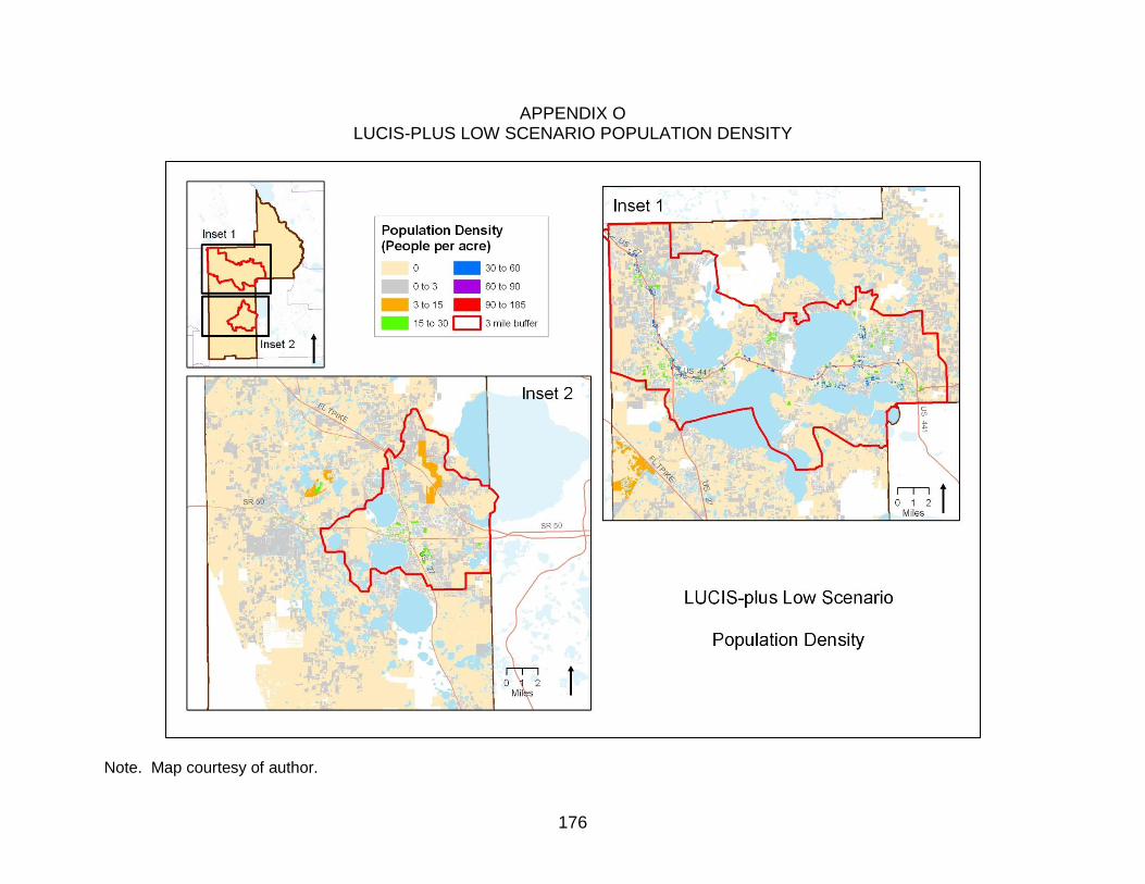
176
APPENDIX O LUCIS-PLUS LOW SCENARIO POPULATION DENSITY
Note. Map courtesy of author.

177
APPENDIX P LUCIS-PLUS HIGH SCENARIO POPULATION DENSITY
Note. Map courtesy of author.

178
APPENDIX Q LUCIS-PLUS LOW SCENARIO EMPLOYMENT DENSITY
Note. Map courtesy of author.

179
APPENDIX R LUCIS-PLUS HIGH SCENARIO EMPLOYMENT DENSITY

180
LIST OF REFERENCES
Bartholomew, K. (2005). Integrating land use issues into transportation planning: Scenario planning. Retrieved March 19, 2010, from http://faculty.arch.utah.edu/bartholomew/SP_SummaryRpt_Web.pdf
Bartholomew, K., & Ewing, R. (2009). Land use-transportation scenarios and future vehicle travel and land consumption: A meta-analysis. Journal of the American Planning Association, 75(1), 13-27.
Bento, A. M., Cropper, M. L., Mobarak, A. M., & Vinha, K. (2005). The effects of urban spatial structure on travel demand in the United States. Review of Economics & Statistics, 87(3), 466-478.
Borning, A., Waddell, P. & Forster, R. (2006). UrbanSim: Using simulation to inform public deliberation and decision-making. Retrieved November 25, 2008, from http://www.cs.washington.edu/homes/borning/papers/borning-urbansim-case-study-2006.pdf
Carbon Dioxide Information Analysis Center. (unknown). Top 20 emitting countries by total fossil-fuel CO2 emissions for 2006. Retrieved February 10, 2010, from http://cdiac.esd.ornl.gov/trends/emis/tre_tp20.html
Chang, J. S. (2006). Models of the relationship between transport and land‐use: A review. Transport Reviews, 26(3), 325-350.
Collins, M.G., Steiner, F.R., & Rushman, M.R. (2001). Land-use suitability analysis in the United States: Historical development and promising technological achievements. Environmental Management, 28(5), 611-621.
Dalton, L. C. (2001). Thinking about tomorrow: Bringing the future to the forefront of planning. Journal of the American Planning Association, 67(4), 397.
Deka, D. (2004). Social and environmental justice issues in urban transportation. In S. Hanson, & G. Guiliano (Eds.), The geography of urban transportation (3rd ed., pp. 332-355). New York: The Guildford Press.
Environmental Systems Research Institute. (2010). ArcGIS desktop 9.3 help. Retrieved March 27, 2010, from http://webhelp.esri.com/arcgisdesktop/9.3/index.cfm?TopicName=welcome
Florida Department of Transportation. (unknown). Florida highway mileage reports - glossary. Retrieved April 1, 2010, from http://www.dot.state.fl.us/planning/statistics/mileage-rpts/glossary.shtm
Florida Department of Transportation. (2005). FSUTMS powered by CUBE/VOYAGER data dictionary. Retrieved March 25, 2010, from http://www.fsutmsonline.net/images/uploads/mtf-files/datadictionary.pdf

181
Florida Department of Transportation. (2009a). MPO program management handbook - Chapter 4: Long-range transportation plan. Retrieved February 8, 2010, from http://www.dot.state.fl.us/planning/policy/metrosupport/mpohandbook/ch4.pdf
Florida Department of Transportation. (2009b). Transit oriented development design guidelines. Retrieved March 27, 2010, from http://www.floridatod.com/docs/Products/TODGuide041409.pdf
Gannett Fleming Inc. (unknown). CFRPMv45 Cube Voyager conversion technical memorandum 1 model conversion procedural guide. Orlando, FL: Florida Department of Transportation District 5.
Handy, S. (2005). Smart growth and the transportation-land use connection: What does the research tell us? International Regional Science Review, 28(2), 146-167.
Handy, S. (2008). Regional transportation planning in the US: An examination of changes in technical aspects of the planning process in response to changing goals. Transport Policy, 15(2), 113-126.
Hanson, S. (2004). The Context of Urban Travel: Concepts and recent trends. In S. Hanson, & G. Guiliano (Eds.), The geography of urban transportation (3rd ed., pp. 3-29). New York: The Guildford Press.
Iacono, M., Levinson, D., & El-Geneidy, A. (2008). Models of transportation and land use change: A guide to the territory. Journal of Planning Literature, 22(4), 323-340.
Isserman, A. (1985). Dare to plan: An essay on the role of the future in planning practice and education. Town Planning Review, 56, 483-491.
Johnston, R. A. (2004). The urban transportation planning process. In S. Hanson, & G. Guiliano (Eds.), The geography of urban transportation (3rd ed., pp. 115-140). New York: The Guildford Press.
Kahyaoğlu-Koračin, J., Bassett, S. D., Mouat, D. A., & Gertler, A. W. (2009). Application of a scenario-based modeling system to evaluate the air quality impacts of future growth. Atmospheric Environment, 43(5), 1021-1028.
Kelly, E. D. (1994). The transportation land-use link. Journal of Planning Literature, 9(2), 128-145.
Kenworthy, J. R. (2003). Transport energy use and greenhouse gases in urban passenger transport systems: A study of 84 global cities. Paper presented at the International third conference of the regional government network for sustainable development, Notre Dame University, Fremantle, Western Australia. Retrieved February 10, 2010, from http://cst.uwinnipeg.ca/documents/Transport_Greenhouse.pdf

182
Knaap, G. (unknown). A requiem for smart growth. Retrieved March 17, 2010, from http://www.smartgrowth.umd.edu/research/pdf/Knaap_Requiem_022305.pdf
Koomen, E., Stillwell, J., Bakema, Aldrik, Scholten, & Henk J. (Eds.). (2007). Modelling land-use change: Progress and applications. The Netherlands: Springer.
Lake County Department of Growth Management. (2009). Lake County, Florida - Comprehensive plan as amended through ordinance #2009-32. Retrieved January 26, 2010, from http://www.lakecountyfl.gov/pdfs/2025/Comp_Plan_as%20of_Ordinance_2009-32.pdf
Lake-Sumter Metropolitan Planning Organization. (2006). Lake-Sumter 2025 long range transportation plan prepared for: Lake-Sumter metropolitan planning organization. Retrieved January 26, 2010, from http://www.lakesumtermpo.com/pdfs/lrtp/lake_sumter_lrtp_complete_052307.pdf
McHarg, I. L. (1992). Design with nature (25 anniversary ed.). New York: J. Wiley.
McNally, M. G. (2007a). The activity-based approach. In K.J. Button & D. A. Hensher (Eds.), Handbook of transport modelling (2nd ed., pp. 53-69). Amsterdam: Elsevier Science.
McNally, M. G. (2007b). The four step model. In K.J. Button & D.A. Hensher, (Eds.), Handbook of transport modelling (2nd ed., pp. 35-52). Amsterdam: Elsevier Science.
Meyer, M. D., & Miller, E. J. (2001). Urban transportation planning: A decision-oriented approach. New York: McGraw-Hill.
Myers, D., & Kitsuse, A. (2000). Constructing the future in planning: A survey of theories and tools. Journal of Planning Education and Research, 19(3), 221-231.
Miller, E. J., Kriger, D. S. & Hunt, J. D. (1998). Integrated urban models for simulation of transit and land-use policies. Retrieved October 10, 2008, from http://www.nap.edu/openbook.php?record_id=9435&page=R1
Muller, P. O. (2004). Transportation and urban form: Stages in the spatial evolution of the American metropolis. In S. Hanson, & G. Giuliano (Eds.), The geography of urban transportation (3rd ed., pp. 59-85). New York: The Guildford Press.
Smith, S. K. (2005). Florida population growth: Past, present and future. Retrieved January 30, 2010, from http://www.bebr.ufl.edu/system/files/FloridaPop2005_0.pdf
183
State of Florida Senate Committee on Community Affairs. (2009). Interim report 2010-107 - Population need as a criteria for changes to a local government's future land use map. Retrieved March 9, 2010, from http://www.fl-counties.com/Docs/Legislative%20Division/Growth%20Management/Population_Need_as_a_Criteria_for_Changes_to_a_Local_Government_s_Future_Land_Use_Map.pdf
Transportation Research Board. (2009). Special Report 298: Driving and the built environment - the effects of compact development on motorized travel, energy use, and CO2 emissions. Washington DC: The National Academies.
Transportation Research Board. (2010). About TRB. Retrieved March 9, 2010, from http://www.trb.org/AboutTRB/Public/AboutTRB.aspx
United Nations Economic Commission for Europe. (2008). Passenger vehicles (number) at 31 December by vehicle category, country and year. Retrieved March 9, 2010, from http://w3.unece.org/pxweb/Dialog/varval.asp?ma=ZZZ_TRvehiclePsgFlit_r&ti=Passenger+Vehicles+%28number%29+at+31+December+by+Vehicle+Category%2C+Country+and+Year&path=../DATABASE/Stat/40-TRTRANS/02-TRRoadFleet/&lang=1
United States Census Bureau. (2000). Profile of selected housing characteristics: 2000 – Census 2000 summary file 3 – Lake County, Florida. Retrieved February 2, 2010, from http://factfinder.census.gov/servlet/QTTable?_bm=y&-geo_id=05000US12069&-qr_name=DEC_2000_SF3_U_DP4&-ds_name=DEC_2000_SF3_U&-_lang=en&-_sse=on
United States Census Bureau. (2000). Profile of selected housing characteristics: 2000 – Census 2000 summary file 3 – Orange County, Florida. Retrieved February 2, 2010, from http://factfinder.census.gov/servlet/QTTable?_bm=y&-geo_id=05000US12095&-qr_name=DEC_2000_SF3_U_DP4&-ds_name=DEC_2000_SF3_U&-_lang=en&-redoLog=false&-_sse=on
United States Census Bureau. (2000). Profile of selected housing characteristics: 2000 – Census 2000 summary file 3 – Osceola County, Florida. Retrieved February 2, 2010, from http://factfinder.census.gov/servlet/QTTable?_bm=y&-geo_id=05000US12097&-qr_name=DEC_2000_SF3_U_DP4&-ds_name=DEC_2000_SF3_U&-_lang=en&-redoLog=false&-_sse=on

184
United States Census Bureau. (2007). Selected housing characteristics: 2005 – 2007 American community survey 3-year estimates – Lake County, Florida. Retrieved October 21, 2009, from http://factfinder.census.gov/servlet/ACSSAFFFacts?_event=&geo_id=05000US12069&_geoContext=01000US|04000US12|05000US12069&_street=&_county=Lake+County&_cityTown=&_state=&_zip=&_lang=en&_sse=on&ActiveGeoDiv=&_useEV=&pctxt=fph&pgsl=050&_submenuId=factsheet_1&ds_name=DEC_2000_SAFF&_ci_nbr=null&qr_name=null®=null%3Anull&_keyword=&_industry=
United States Census Bureau. (2008). Journey to work and place of work - Census 2000 data - 2000 County to county worker flow files. Retrieved January 30, 2010, from http://www.census.gov/population/www/cen2000/commuting/index.html#FL
United States Census Bureau. (2008). Selected housing characteristics: 2008 – 2008 American community survey 1-year estimates – Lake County, Florida. Retrieved February 2, 1010, from http://factfinder.census.gov/servlet/ADPTable?_bm=y&-geo_id=05000US12069&-qr_name=ACS_2008_1YR_G00_DP4&-context=adp&-ds_name=&-tree_id=308&-_lang=en&-redoLog=false&-format=
United States Census Bureau. (2008). Selected housing characteristics: 2008 – 2008 American community survey 1-year estimates – Orange County, Florida. Retrieved February 2, 1010, from http://factfinder.census.gov/servlet/ADPTable?_bm=y&-context=adp&-qr_name=ACS_2008_1YR_G00_DP4&-ds_name=ACS_2008_1YR_G00_&-tree_id=308&-redoLog=true&-_caller=geoselect&-geo_id=05000US12095&-format=&-_lang=en
United States Census Bureau. (2008). Selected housing characteristics: 2008 – 2008 American community survey 1-year estimates – Osceola County, Florida. Retrieved February 2, 1010, from http://factfinder.census.gov/servlet/ADPTable?_bm=y&-context=adp&-qr_name=ACS_2008_1YR_G00_DP4&-ds_name=ACS_2008_1YR_G00_&-tree_id=308&-redoLog=true&-_caller=geoselect&-geo_id=05000US12097&-format=&-_lang=en
United States Environmental Protection Agency, Office of Research and Development. (2000). Projecting land-use change: A summary of models for assessing the effects of community growth and change on land-use patterns (Report No. EPA/600/R-00/098). Cincinnati, OH: U.S. EPA.
United States Environmental Protection Agency. (2009). Human-related sources and sinks of carbon dioxide. Retrieved February 10, 2010, from http://www.epa.gov/climatechange/emissions/co2_human.html

185
United States Government Accountability Office. (2007). Crude oil: Uncertainty about future oil supply makes it important to develop a strategy for addressing a peak and decline in oil production (Report No. GA-07-283). Washington DC: United States Government Accountability Office.
University of Florida Bureau of Economic and Business Research, & University of Florida Population Program. (2009). Florida population studies bulletin 153 - Florida county population projections, 2008 - 2035. Gainesville, FL: Bureau of Economic and Business Research, College of Business Administration, University of Florida.
Wachs, M. (2001). Forecasting versus envisioning: A new window on the future. Journal of the American Planning Association, 67(4), 367-72.
Wachs, M. (2004). Reflections on the planning process. In S. Hanson, & G. Guiliano (Eds.), The geography of urban transportation (3rd ed., pp. 141-162). New York: The Guildford Press.
Waddell, P., & Ulfarsson, G. F. (2004). Introduction to urban simulation: Design and development of operational models. In P. Stopher, K. Button, K. Haynes & D. Hensher (Eds.), Handbook of transport volume 5: Transport geography and spatial systems (pp. 203-236) Pergamon Press.
Weitz, J. (1999). From quiet revolution to smart growth: State growth management programs, 1960 to 1999. Journal of Planning Literature, 14(2), 266-337.
Wilbur Smith Associates. (2008). Lake County transit development plan - 2008 major update. Retrieved February 4, 2010, from http://www.lakesumtermpo.com/pdfs/tdp/Lake_County_2020_TDP_adopted0808.pdf
Zegras, C., Sussman, J., & Conklin, C. (2004). Scenario planning for strategic regional transportation planning. Journal of Urban Planning and Development, 130(1), 2-13.
Zhao, F., & Chung, S. (2006). A study of alternative land use forecasting models (Final Report No. BD015-10). Tallahassee, FL: Florida Department of Transportation.

186
BIOGRAPHICAL SKETCH
Liz Thompson was born in 1963 in Camp Hill, Pennsylvania. Her family emigrated
to Perth, Western Australia in 1971 where she lived until returning to live in the United
States in 2003. Liz is currently pursuing a Master of Arts degree in Urban and Regional
Planning at the University of Florida, in Gainesville. She has a Bachelor of Arts degree
in geography and history from the University of Western Australia. As a graduate
student at the University of Florida, Liz worked as a research assistant for Dr. Paul
Zwick assisting in the continuing development of the Land Use Conflict Identification
Strategy (LUCIS), work that she will continue after her graduation in summer 2010. Liz
began working for the Shimberg Centre for Housing Studies in April 2010 where her
proficiency in geographic information systems is assisting in the development of the
Florida Neighborhood Data Initiative (FNDI) which aims to support affordable housing
and community revitalization.
Liz met Kevin Thompson in 1994 during a five-year working holiday that began in
1992 and traversed Japan, the United States, Taiwan, and New Zealand. In 1996, they
moved to Liz‟s home town of Perth, Western Australia. In 2002, they married and later
that year their beautiful daughter Amelie Helen was born. They returned to live in the
USA in 2003, moving to Gainesville, Florida in 2007 where they continue to reside.