environmental engineering solutions; stress path ... · pdf filesolution for the wellbore...

Draft

Drained and undrained analyses of cylindrical cavity

contractions by Bounding Surface plasticity

Journal: Canadian Geotechnical Journal

Manuscript ID cgj-2015-0605.R2

Manuscript Type: Article

Date Submitted by the Author: 20-Apr-2016

Complete List of Authors: Chen, Shengli; Louisiana State University System, Department of Civil & Environmental Engineering Abousleiman, Younane; The University of Oklahoma

Keyword: cylindrical cavity contraction; bounding surface model; semi-analytical solutions; stress path; tunnelling; wellbore drilling

https://mc06.manuscriptcentral.com/cgj-pubs

Canadian Geotechnical Journal

Draft

1

DRAINED AND UNDRAINED ANALYSES OF CYLINDRICAL CAVITY

CONTRACTIONS BY BOUNDING SURFACE PLASTICITY

S. L. Chen, and Y. N. Abousleiman

S. L. Chen, Department of Civil & Environmental Engineering, Louisiana State University,

Baton Rouge, LA, USA. Email: [email protected]

Y. N. Abousleiman, Integrated PoroMechanics Institute, ConocoPhillips School of Geology and

Geophysics, Mewbourne School of Petroleum & Geological Engineering, The University of

Oklahoma, Norman, OK, USA. Email: [email protected]

Page 1 of 52



Draft

2

Abstract: This paper develops a rigorous semi-analytical approach for drained/undrained

cylindrical cavity contraction problems in bounding surface elastoplastic geomaterials. For

undrained situation, the effective radial, tangential, and vertical component stresses can be

directly solved from the constitutive governing differential equations as an initial value problem,

the excess pore pressure subsequently being determined from the radial equilibrium equation.

Whereas for the drained case, the Eulerian radial equilibrium equation must be first transformed

into an equivalent one in Lagrangian description via the introduction of an auxiliary variable, and

then be solved together with the elastoplastic constitutive relation for the three stress components

as well as the specific volume. It is observed that during drained/undrained contraction

processes, plastic deformations occur immediately as a direct result of employing the bounding

surface model, so outside the cavity there exists no purely elastic zone. The computed stress

distributions and in particular the stress path prediction through an example analysis capture well

the anticipated elastoplastic and failure behaviour of the geomaterials surrounding the cavity.

The validity and accuracy of the proposed semi-analytical elastoplastic solutions are justified

through comparison with ABAQUS numerical results, and its applicability to the tunnel

excavation and wellbore drilling problems is also demonstrated.

Keywords: cylindrical cavity contraction; bounding surface model; semi-analytical solutions;

stress path; tunnelling; wellbore drilling

Page 2 of 52



Draft

3

Introduction

The cavity contraction theory has wide applications to the design and construction of

tunnels in civil engineering and to the stress and displacement modelling around the drilled

wellbore in petroleum engineering as well. However, in contrast to the cavity expansion problem

(Gibson and Anderson 1961; Vesic 1972; Randolph et al. 1979; Carter et al. 1986; Yu 1990;

Collins and Stimpson 1994; Salgado and Randolph 2001; Russell and Khalili 2006), much less

investigations of cavity contraction in soil and rock have been conducted, which is particularly

the case when the critical state plasticity models (Wood 1990; Dafalias and Herrmann 1980) are

involved.

Stress and strain analyses for the cavity contraction problem incorporating elasoplastic

behaviour of geomaterials usually are obtained through numerical methods (Carter 1978; Potts

and Zdravkovic 1999). So far scarce analytical/semi-analytical plasticity solutions exist in the

literature for such fundamental problem even when major approximations are assumed. The

earlier analytical contributions to the tunnel/wellbore opening problems usually modelled the

soil/rock as associated or non-associated elastic-perfectly plastic materials like linear Mohr-

Coulomb and nonlinear Hoek-Brown yield criteria (Brown et al. 1983), and under isotropic in

situ stress condition. Later Graziani and Ribacchi (1993) proposed an analytical approach to

determine the state of stress and strain for a circular opening excavated in a rock mass, where the

rock is assumed to obey the non-associated strain softening Mohr-Coulomb model with the

softening behaviour linked to a simple plastic shear strain through the so-called softening

modulus parameter. Papanastasiou and Durban (1997) made a further substantial extension to the

cylindrical cavity solutions for Drucker-Prager and Mohr-Coulomb geomaterials exhibiting

arbitrary strain hardening behaviour. However, for the case of Mohr-Coulomb model in

Page 3 of 52



Draft

4

Papanastasiou and Durban (1997), the assumption of the axial stress being the intermediate

principal stress is not necessarily true during the cavity expansion/contraction and may easily

violate the plane strain condition in the axial direction (Reed 1988; Yu and Rowe 1999).

In addition to the Drucker-Prager, Mohr-Coulomb, and Hoek-Brown models (the latter two

are quite suitable for modelling the granular geomaterials as they capture reasonably well the

particle rearrangement and the frictional sliding between material particles), the analytical cavity

contraction solutions based on the critical state plasticity models have also been developed,

though quite limited. For example, Charlez and Roatesi (1999) derived an approximate analytical

solution for the wellbore stability problem under undrained condition using a very simplistic,

idealized Cam Clay model where the elliptical yield surface was replaced by two straight lines,

and the solution is restricted to the volumetric strain hardening rocks with overconsolidation

ratio less than 2. Concurrently, Yu and Rowe (1999) provided a set of comprehensive yet still

approximate analytical/semi-analytical solutions for the undrained circular excavation problem

using the well known Cam Clay critical state theories (Wood 1990). Nevertheless, as noted in

Chen and Abousleiman (2012; 2013), the main drawback in their approach is that the deviatoric

and mean effective stresses were treated in some approximate fashion by enforcing both the two

stress invariants independent of the axial stress, simply to obtain the possible closed form

solutions.

This paper considers the cavity contraction boundary value problem involving the bounding

surface plastic model (Dafalias and Herrmann 1980; 1982), under both undrained and drained

conditions. The prominent feature of this critical state based model, with the seminal concept of

the bounding surface in stress space, is that inelastic deformation can occur for stress points

within the bounding surface at a pace depending on the proximity of the current stress state to the

Page 4 of 52



Draft

5

bounding surface (Kaliakin et al. 1987), so that the realistic non-recoverable behaviour of

soils/rocks observed on unloading and reloading can be well recovered. As with Chen and

Abousleiman (2012; 2013), the key step in the formulation of cavity contraction in geomaterials

using bounding surface plasticity model is to establish an appropriate incremental relationship

between the effective radial, tangential, and vertical stresses and the corresponding stain

components, i.e., the elastoplastic constitutive equations, and then reduce them to a set of

differential equations valid for any material point in the plastic zone. For undrained condition,

the three stresses can be directly solved from these governing differential equations as an initial

value problem, the excess pore pressure then being determined from the radial equilibrium

equation. Whereas for the drained condition, the Eulerian radial equilibrium equation must be

first transformed into an equivalent one in Lagrangian description, which can be accomplished

with the introduction of an auxiliary variable. This transformed equation, together with the

aforementioned elastoplastic constitutive relation, again constitute a set of differential equations.

The three stress components as well as the specific volume thus can be readily solved. The

computed stress distributions and in particular the stress path prediction through an example

analysis, for different values of overconsolidation ratio (��) , capture well the anticipated

elastoplastic to failure behaviour of the soils/rocks surrounding the cavity. As an application to

the practical tunnel and wellbore opening problems, the semi-analytical elastoplastic solutions

developed is utilized to predict the critical support pressure that is required to maintain the

tunnel/wellbore stability.

Bounding surface model

The well established bounding surface concept was originally introduced by Dafalias and

Popov (1975; 1976) and later on reformulated within the framework of critical state soil

Page 5 of 52



Draft

6

plasticity by Dafalias and Herrmann (1980; 1982; 1986). The basic idea of their formulation is

that an isotropically expanding or contracting surface, rather than a yield surface, is used in the

model. This surface is known as the bounding surface which depends only on the plastic

volumetric strain (or plastic void ratio). In addition, the bounding surface model uses a simple

radial mapping to determine a unique image point on the bounding surface that corresponds to

the current stress point inside the bounding surface. The value of the plastic modulus is assumed

to be a function of the distance between the stress point and its image, while the gradient of the

bounding surface at the image point defines the loading-unloading direction. The salient feature

of this model is that plastic deformation may occur for stress point even inside the surface.

Fig. 1 shows a schematic illustration of the bounding surface model. A stress state �� lies

always within or on the bounding surface which, mathematically, can be expressed as

�� , �� = 0 (1)

where a bar over effective stress quantities �� indicates points on the bounding surface �� = 0,

and �� , the plastic void ratio, is the only plastic internal variable defining the

hardening/softening behaviour of the bounding surface. Note that the plastic void ratio �� is

related to the plastic volumetric strain �� and the elastic void ratio �� as follows

�� = −(1 + �)�� (2)

�� + �� = � − �� (3)

where � is the total void ratio; � is the specific volume (� = 1 + �); �� is the initial specific

volume; and �� and �� are the increments of plastic void ratio and plastic volumetric strain,

respectively. It should be pointed out that in Eq. (2) the current (varying) void ratio �, instead of

the initial void ratio �� (Dafalias and Herrmann 1980; 1986), has been adopted for a rigorous

definition of ��. This will be able to more suitably accommodate the large plastic deformations

Page 6 of 52



Draft

7

of the geomaterials that most likely occur during the cavity contraction process.

In addition to the bounding surface, at any stress point �� a surface homeothetic to the

bounding surface with respect to the origin � can be indirectly defined (shown by a dashed line

in Fig. 1)

� �� = 0 (4)

Such a surface is referred to as the loading surface in Dafalias and Herrmann (1980; 1982),

which specifies a quasi-elastic domain but is actually not a yield surface since an inward motion

of �� will eventually induce loading after an initial path of unloading before �� reaches the

surface again.

The plastic constitutive relations for the bounding surface model, in the general stress space,

can be expressed as (Dafalias and Herrmann 1980)

�� = ⟨�⟩ � (5)

� = !" ��#$ #$ = !"& ��#$ #$ (6)

where � (or #$ ) denotes the unit normal at stress point �� or its image point �� on the

bounding surface, see Fig. 1; ' is the actual plastic modulus associated with ��#$ ; '( is a plastic

modulus on the bounding surface associated with ��#$ ; the Macauley bracket ⟨·⟩ define the

operation ⟨�⟩ = ℎ(�) · � , ℎ being the heaviside step function; � is usually called the loading

function. The bounding surface plastic modulus '( is obtained from the consistency condition

�� = +,�+-./01 �� + +,�+�2 �� = 0 (7)

with the aid of Eq. (2), as follows

'( = !3�4 56.57./01 · 56.57./01 8

+,�+�2 +,�+-.991 (8)

Page 7 of 52



Draft

8

Note that in the above two equations the summation convention over repeated indices applies.

The plastic modulus ' needed to determine the plastic strain increment at the current stress

point �� is related to '( by

' = '( + :(�� , ��) ;;<=-/01 ,�2>?; (9)

where : is the hardening function; @ is the distance between �� and �� ; and @� is a properly

chosen reference stress.

Elastoplastic constitutive equations

It must be emphasized that the major objective of this paper is to provide a rigorous semi-

analytical solution for the cavity contraction boundary value problem in generic boundary

surface soils/rocks, instead of focusing on the constitutive model itself. Therefore, to simplify the

formulation yet still retaining the essential ingredients of the bounding surface plasticity

(Dafalias and Herrmann 1980; 1982; 1986; Kaliakin and Dafalias 1989; Manzari and Nour

1997), the initial and specific version of the bounding surface model by Dafalias and Herrmann

(1980) will be chosen for the cavity analysis. The bounding surface is further assumed to consist

of one single ellipse (Kaliakin and Dafalias 1989; Manzari and Nour 1997), as shown in Fig. 1.

However, the formulation and derivation presented in this work, with little or minor

modification, shall be applicable to the “composite” surface consisting of two ellipses and a

hyperbola (Dafalias and Herrmann 1980; 1982; 1986) and later improved versions of the

bounding surface models as well involving three stress invariants (Dafalias and Herrmann 1986)

and more sophisticated hardening function : (Kaliakin and Dafalias 1989).

In accordance with Dafalias and Herrmann (1980; 1986), the bounding and loading

surfaces, �� and � (see Fig. 1), can be expressed as

Page 8 of 52



Draft

9

�� , �� ≡ ��(B̅, D�, ��) = E�̅1�̅F1GH + (I?!)JKJ E L��̅F1GH − HI �̅1�̅F1 + H?II = 0 (10)

� �� ≡ �(B, D) = =�1�M1 >H + (I?!)JKJ = L�M1 >H − HI �1�M1 + H?II = 0 (11)

where

B = !N (�O + �P + �Q) (12a)

B̅ = !N (��O + ��P + ��Q) (12b)

D = R!H S(�O − �P )H + (�O − �Q)H + (�P − �Q)HT (13a)

D� = R!H S(��O − ��P )H + (��O − ��Q)H + (��P − ��Q)HT (13b)

with �O , �P , �Q and ��O , ��P , ��Q denoting, respectively, the actual and image effective radial,

tangential, and vertical stresses, which are the three principal stresses for axisymmetric

cylindrical cavity problem and considered positive here for compression; U is the slope of

critical state line; � is a constant model parameter and essentially defines the shape of the

bounding surface; B̅V represents the intersection of the current bounding surface with the B axis,

which is, in fact, the value of B for isotropic consolidation and is connected with the plastic

volumetric strain by

W�̅F1�̅F1 = (!3�)X?Y �� (14)

where Z and [ are the slopes of normal compression and swelling lines in � − lnB plane (Wood

1990); and B̂ is determined as the intersection between the loading surface passing through the

current stress point (B, D) and the B′ axis.

According to Eqs. (4)-(6) and (11), the three components of incremental plastic strain can

be expressed as

Page 9 of 52



Draft

10

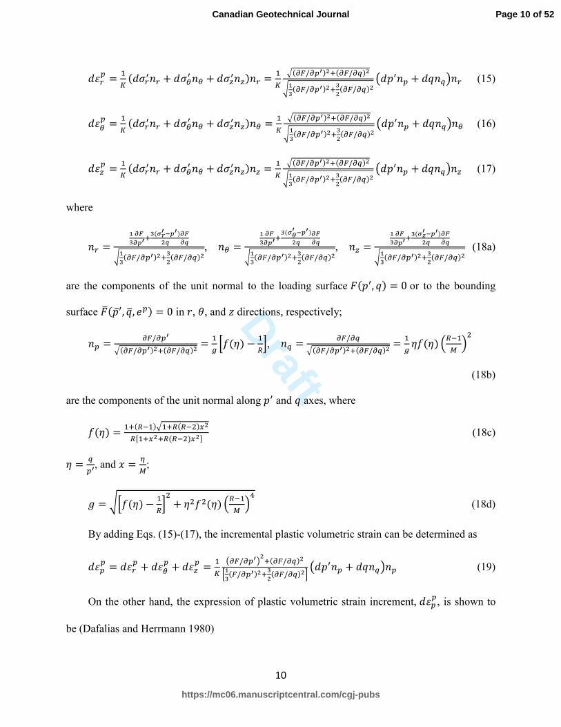
��O� = !" (��O O + ��P P + ��Q Q) O = !" `(+,/+�1)J3(+,/+L)JRbc(+,/+�1)J3cJ(+,/+L)J �B � + �D L� O (15)

��P� = !" (��O O + ��P P + ��Q Q) P = !" `(+,/+�1)J3(+,/+L)JRbc(+,/+�1)J3cJ(+,/+L)J �B � + �D L� P (16)

��Q� = !" (��O O + ��P P + ��Q Q) Q = !" `(+,/+�1)J3(+,/+L)JRbc(+,/+�1)J3cJ(+,/+L)J �B � + �D L� Q (17)

where

O = bc 565213c(7d1e21)Jf 565fRbc(+,/+�1)J3cJ(+,/+L)J, P =

bc 565213c(7g1 e21)Jf 565fRbc(+,/+�1)J3cJ(+,/+L)J, Q =

bc 565213c(7h1e21)Jf 565fRbc(+,/+�1)J3cJ(+,/+L)J (18a)

are the components of the unit normal to the loading surface �(B, D) = 0 or to the bounding

surface ��(B̅, D�, ��) = 0 in i, j, and k directions, respectively;

� = +,/+�1`(+,/+�1)J3(+,/+L)J = !l mn(o) − !Ip, L = +,/+L`(+,/+�1)J3(+,/+L)J = !l on(o) =I?!K >H

(18b)

are the components of the unit normal along B and D axes, where

n(o) = !3(I?!)`!3I(I?H)qJIr!3qJ3I(I?H)qJs (18c)

o = L�1, and t = uK;

v = Rmn(o) − !IpH + oHnH(o) =I?!K >w (18d)

By adding Eqs. (15)-(17), the incremental plastic volumetric strain can be determined as

�� = ��O� + ��P� + ��Q� = !" +,/+�1�J3(+,/+L)Jmbc(,/+�1)J3cJ(+,/+L)Jp �B � + �D L� � (19)

On the other hand, the expression of plastic volumetric strain increment, ��, is shown to

be (Dafalias and Herrmann 1980)

Page 10 of 52



Draft

11

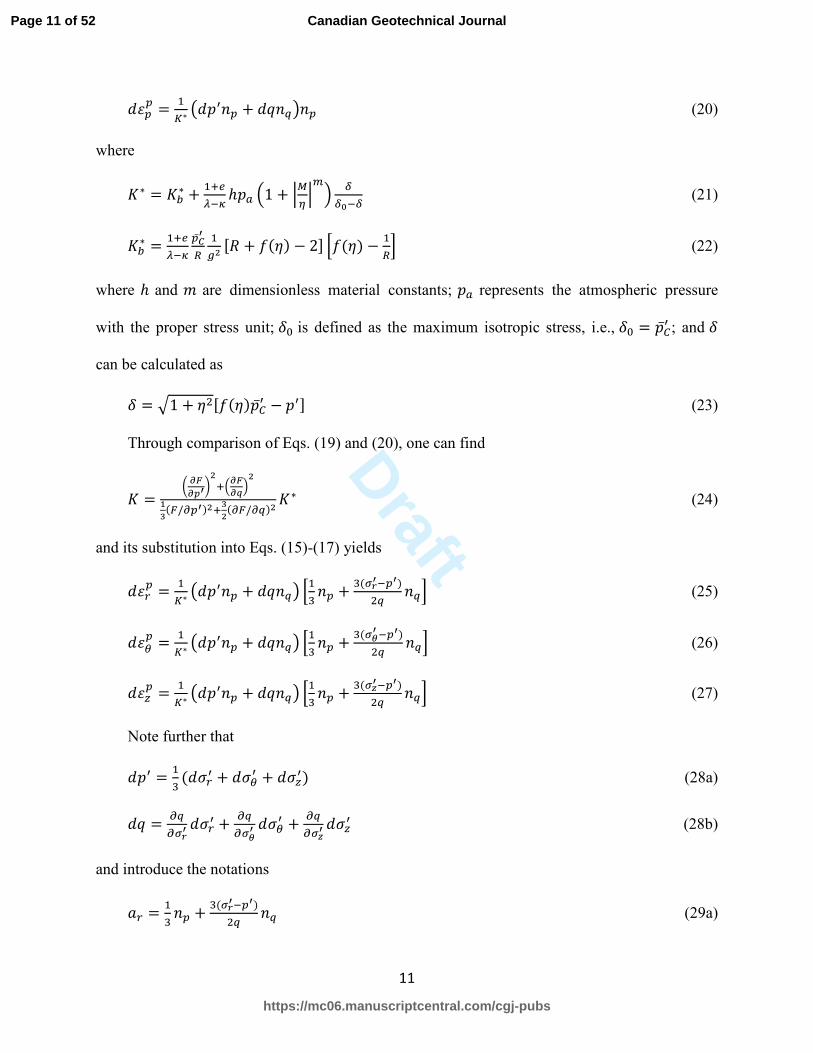
�� = !"∗ �B � + �D L� � (20)

where

'∗ = '(∗ + !3�X?Y ℎBy =1 + zKu z{> ;;<?; (21)

'(∗ = !3�X?Y �̅F1I !lJ r� + n(o) − 2s mn(o) − !Ip (22)

where ℎ and | are dimensionless material constants; By represents the atmospheric pressure

with the proper stress unit; @� is defined as the maximum isotropic stress, i.e., @� = B̅V ; and @

can be calculated as

@ = `1 + oHrn(o)B̅V − Bs (23)

Through comparison of Eqs. (19) and (20), one can find

' = E 56521GJ3=565f>Jbc(,/+�1)J3cJ(+,/+L)J'∗ (24)

and its substitution into Eqs. (15)-(17) yields

��O� = !"∗ �B � + �D L� m!N � + N(-d1?�1)HL Lp (25)

��P� = !"∗ �B � + �D L� m!N � + N(-g1?�1)HL Lp (26)

��Q� = !"∗ �B � + �D L� m!N � + N(-h1?�1)HL Lp (27)

Note further that

�B = !N (��O + ��P + ��Q) (28a)

�D = +L+-d1 ��O + +L+-g1 ��P + +L+-h1 ��Q (28b)

and introduce the notations

}O = !N � + N(-d1?�1)HL L (29a)

Page 11 of 52



Draft

12

}P = !N � + N(-g1?�1)HL L (29b)

}Q = !N � + N(-h1?�1)HL L (29c)

the plastic stress strain response can therefore be written in a matrix form

~��O�

��P��Q�� = !"∗ � }OH }O}P }O}Q}P}O }PH }P}Q}Q}O }Q}P }QH � · ~��O��P��Q� (30)

It should be remarked here that }O, }P, }Q, and '∗ on the right hand side of the above equation

all could be explicitly expressed as functions of the three stress components �O , �P , and �Q , which is of vital importance to ensure an analytical solution for the cavity contraction

elastoplastic boundary value problem. Such a desirable feature for the plastic modulus '∗ will be

demonstrated in the next section.

On the other hand, the elastic stress strain relationship can be written in incremental form as

~��O��P��Q�� = !� 4 1 −� −�−� 1 −�−� −� 1 8 · ~��O��P��Q� (31)

where ��O�, ��P�, and ��Q� are the elastic strain increments in i, j, and k directions, respectively;

� is the Poisson's ratio; and the Young's modulus � [or shear modulus � = �H(!3�)], is a function

of the mean stress B and specific volume �:

� = N(!?H�)��1Y (32)

Combining Eqs. (30) and (31), and by inverting, one finally has the following elastoplastic

constitutive equations for the bounding surface model

~��O��P��Q� = !� 4�!! �!H �!N�H! �HH �HN�N! �NH �NN8 · ��O��P��Q� (33)

Page 12 of 52



Draft

13

where

�!! = !�J m1 − �H + �}PH !"∗ + 2��}P}Q !"∗ + �}QH !"∗p (34a)

�!H = !�J m−�}O(}P + �}Q) !"∗ + �(1 + � − �}P}Q !"∗ + �}QH !"∗)p (34b)

�!N = !�J m−�}O(�}P + }Q) !"∗ + �(1 + � + �}PH !"∗ − �}P}Q !"∗)p (34c)

�HH = !�J m1 − �H + �}OH !"∗ + 2��}O}Q !"∗ + �}QH !"∗p (34d)

�HN = !�J m� + �H + ��}OH !"∗ − �}P}Q !"∗ − ��}O(}P + }Q) !"∗p (34e)

�NN = !�J m1 − �H + �}OH !"∗ + 2��}O}P !"∗ + �}PH !"∗p (34f)

�H! = �!H (34g)

�N! = �!N (34h)

�NH = �HN (34i)

� = − !3��c m(−1 + � + 2�H) + �(−1 + �)}OH !"∗ + �(−1 + �)}PH !"∗ − 2��}P}Q !"∗

−�}QH !"∗ + ��}QH !"∗ − 2��}O(}P + }Q) !"∗p (34j)

Cavity contraction boundary value problem

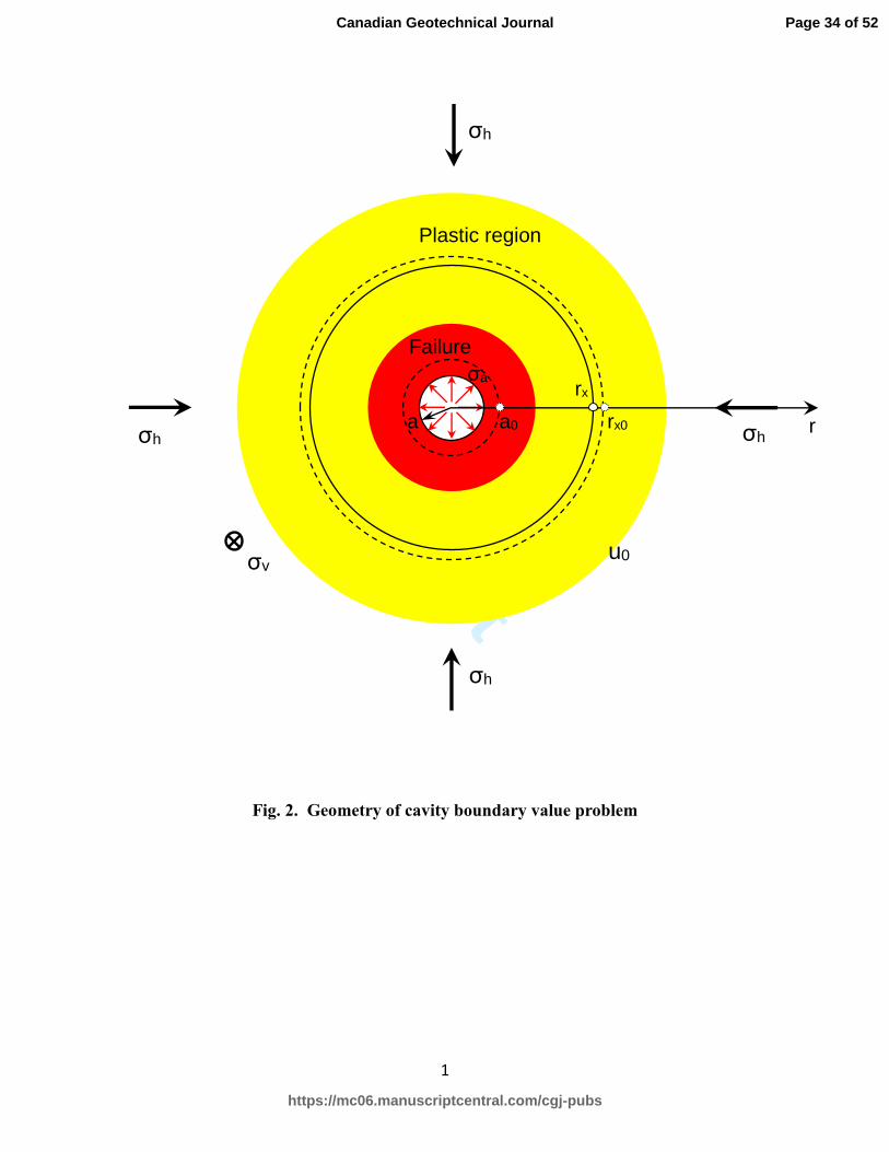
The scenario of cylindrical cavity contraction in an infinite elastoplastic porous medium is

shown in Fig. 2. Initially the geomaterial is subjected to an in-plane (horizontal) stress ��, an

out-of-plane (vertical) stress ��, and a pore pressure ��, respectively. The cavity has an initial

radius }� and is contracted to the current radius } when the cavity pressure is decreased from ��

to �y. At this instant a typical particle initially at radial distance iq� will have moved inward to a

new position denoted by iq.

It is noteworthy that for a cavity contracted in a bounding surface geomaterial, plastic

Page 13 of 52



Draft

14

deformations occur immediately for all the material particles, after the reduction of the internal

cavity pressure, so there is no elastic zone existing around the cavity, see Fig. 2. This is the direct

result of employing bounding surface model for which as described earlier yielding may occur as

soon as loading commences in the stress space.

UNDRAINED CASE

For undrained condition,

�� = �� + �� = 0 (35)

where �� denotes the elastic volumetric strain increment and, from Eqs. (31) and (32), can be

expressed as

�� = ��O� + ��P� + ��Q� = YW�1��1 (36)

Substituting Eq. (36) into Eq. (14) yields

W�̅F1�̅F1 = − (!3�)X?Y �� = − YX?Y W�

1�1 (37)

which, after integration, gives

B̅V = B̅V,� =�1�<1>?��e�

(38)

Here B� corresponds to the initial mean effective stress and B̅V,� is the initial value of B̅V before

the contraction of cavity. Eq. (38) shows clearly that B̅V , the size of the bounding surface, is

expressible with respect to the current stress state B, and hence to the three stress components.

This in conjunction with Eqs. (21)-(22) indicates that '∗ can also be explicitly expressed in

terms of �O, �P , and �Q only, an ascertainment having been made indeed in the previous section.

Note that in Fig. 1, B̂ is determined as the intersection between an ellipse passing through

the current stress point (B, D) and the B′ axis. Its initial value of B^,� relevant to the initial stress

Page 14 of 52



Draft

15

state (B� , D�), together with B̅V,� , thus define the useful concept of overconsolidation ratio for the

soils and rocks

�� = �̅F,<1�M,<1 (39)

For undrained cylindrical cavity contraction problem �� = 0, and also ��Q = 0 as a result

of plane strain deformation, the incremental radial and tangential logarithmic strains thus can be

expressed as (Chen and Abousleiman 2012)

��O = −��P = WOO (40)

where i is the radial coordinate associated with a given material particle and �i is the

infinitesimal change in position of that particle (Lagrangian description). Turning back to the

elastoplastic constitutive equation (33), one obtains three first order governing differential

equations with the three stress unknowns being functions of single variable i as follows

�-d1�O − (bb?(bJ�O = 0 (41a)

�-g1�O − (Jb?(JJ�O = 0 (41b)

�-h1�O − (cb?(cJ�O = 0 (41c)

where ��O denotes the material derivative taken along the particle motion path (Lagrangian

description).

The final point that needs to be addressed now is the specification of suitable initial

conditions for the above differential equations. Recall that, for the bounding surface model, there

is no purely elastic deformation zone existing around the cavity. Therefore, Eqs. (41a)-(41c) are

in principle valid for any material point with current position iq, whose original position, iq�, can

be identified from the kinematic constraint of undrained deformation as

Page 15 of 52



Draft

16

O�<y = R=O�y >H + =y<y >H − 1 (42)

and the corresponding initial stress conditions are simply given by

�O(iq�) = �O� = �� − ��, �P (iq�) = �P� = �� − ��, �Q(iq�) = �Q� = �� − �� (43)

where �O� ,�P� , and�Q� are the initial effective stresses.

Once the effective stresses are solved from Eqs. (41a)-(41c), subject to the initial condition

(43), the distribution of pore pressure �(iq) can be easily calculated from the equilibrium

equation

+-d1+O + +�+O + -d1?-g1O = 0 (44)

and the excess pore pressure then determined from

Δ�(iq) = �(iq) − �� (45)

DRAINED CASE

When the cavity is contracted under drained condition, the pore pressure � is eventually

constant equal to the initial value of �� and can be subtracted out of the analysis. The equilibrium

equation (44) therefore reduces to

+-d1+O + -d1?-g1O = 0 (46)

For the drained situation, the elastoplastic stress strain response, Eq. (33), is still valid as the

constitutive relation for geomaterials is formulated based on the concept of effective stresses.

However, it should be pointed out that in this case the void ratio � (or specific volume �), is no

longer a constant but instead changes with the deformation so itself needs to be determined

during the contraction process. The influences of varying � (or �) are well reflected in Eqs. (21)

and (22) for the plastic moduli '∗ and '(∗. Additionally, it will affect indirectly the hardening

Page 16 of 52



Draft

17

parameter B̅V which essentially controls the size of the current bounding surface. As a matter of

fact, Eq. (38) for the determination of B̅V is no longer applicable for the drained case since this

equation is derived based on the constant specific volume condition, �� = 0.

Consider now the expression of B̅V for the drained condition. Substituting Eq. (2) into (14),

and integrating, gives

ln �̅F1�̅F,<1 = − !X?Y �� (47)

Using Eq. (3), thus,

ln �̅F1�̅F,<1 = − !X?Y (� − �� − � �� ) (48)

Here

� �� = � −(1 + �)�� = � −(1 + �) W�1∙Y(!3�)�1 = −[ln �1�<1�� (49)

so that

�̅F1�̅F,<1 = �?�e�<�e� (�1�<1)? ��e� (50)

which again expresses B̅V as an explicit function of the current stress state as well as the current

specific volume �, and so does the plastic moduli '∗ from Eqs. (21)-(22). Note that when � =��, the above equation correctly reduces to Eq. (38) for the undrained case.

Let us now move on to the formulation of the governing differential equations for the

drained condition. Given the elastoplastic incremental constitutive relation, Eq. (33), and noting

that �� = − W�� and ��P = − WOO , it follows that

��O = !� r�!!�� + (�!H − �!!)��Ps = !� r�!!(− W�� ) + (�!H − �!!)(− WOO )s (51a)

��P = !� r�H!�� + (�HH − �H!)��Ps = !� r�H!(− W�� ) + (�HH − �H!)(− WOO )s (51b)

��Q = !� r�N!�� + (�NH − �N!)��Ps = !� r�N!(− W�� ) + (�NH − �N!)(− WOO )s (51c)

Page 17 of 52



Draft

18

Introduce an auxiliary independent variable �, defined as

� = �dO = O?O<O (52)

with �O known as the radial displacement and i� the original position of the particle, and then

follow the same procedure as outlined in Chen (2012) for the drained cavity analysis, one can

finally derive the desirable four governing differential equations

�-d1�� = − -d1?-g1!?�? �<�(be�) (53a)

�-g1�� = − (Jb(bb � -d1?-g1!?�? �<�(be�) + (bb?(bJ�(!?�) � − (JJ?(Jb�(!?�) (53b)

�-h1�� = − (cb(bb � -d1?-g1!?�? �<�(be�)+ (bb?(bJ�(!?�) � − (cJ?(cb�(!?�) (53c)

�� = ��(bb � -d1?-g1!?�? �<�(be�) + (bb?(bJ�(!?�) � (53d)

which can be solved for any material particle iq as an initial value problem with the independent

variable starting at � = �� = 0. As in the undrained case, the initial conditions for stresses and

specific volume are simply as follows

�O(0) = �O� , �P (0) = �P� , �Q(0) = �Q� , �(0) = �� (54)

Obviously, the above differential equations (53a)-(53d) are expressed with respect to the

auxiliary variable � rather than the radial coordinate i. To complete the solutions, it is therefore

necessary to establish a link between � and i, which can be found as (Chen and Abousleiman

2013)

Oy = �� be �<�(�)(be�)e�

��(�) (55)

Page 18 of 52



Draft

19

Results and discussions

The parameters of the bounding surface model used for both undrained and drained cavity

contraction analyses are � = 2.72, U = 1.05, Z = 0.14, [ = 0.05, � = 0.15, �� = 0.95(�� =1.95), | = 0.2, and ℎ = 30, as listed in Table 1. Four different values of �� = 1, 1.2, 2, and

5 are considered to investigate the impact of overconsolidation ratio on the stress and pore

pressure distributions around the cavity. The in situ effective stresses and pore pressure, as well

as the relevant values of B̅V,� are also summarized in Table 1.

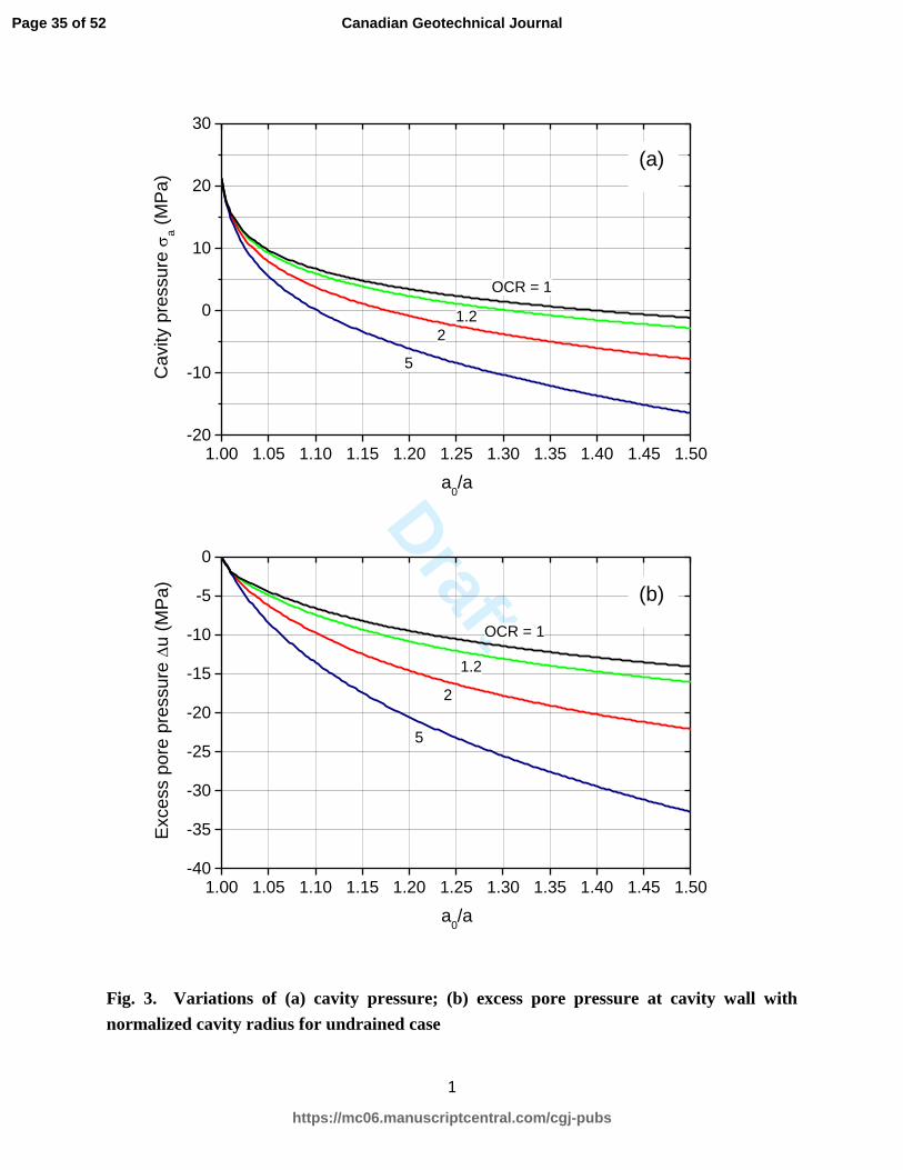
Fig. 3 shows the variations of the internal support pressure �y (compression positive) and

excess pore pressure ∆�(}) at cavity wall i = } with the normalized cavity radius y<y , generally

known as the tunnel characteristic curve and wellbore closure curve, for the undrained case and

for �� = 1, 1.2, 2, and 5. It is seen that the cavity pressure decreases significantly as ��

increases from 1 for normally consolidated geomaterial to 5 for heavily overconsolidated

geomaterial. Similar trends can also be observed for the excess pore pressure build-up in Fig. 3a,

where the negative result of ∆� gives a clear indication of the decrease in total pore pressure.

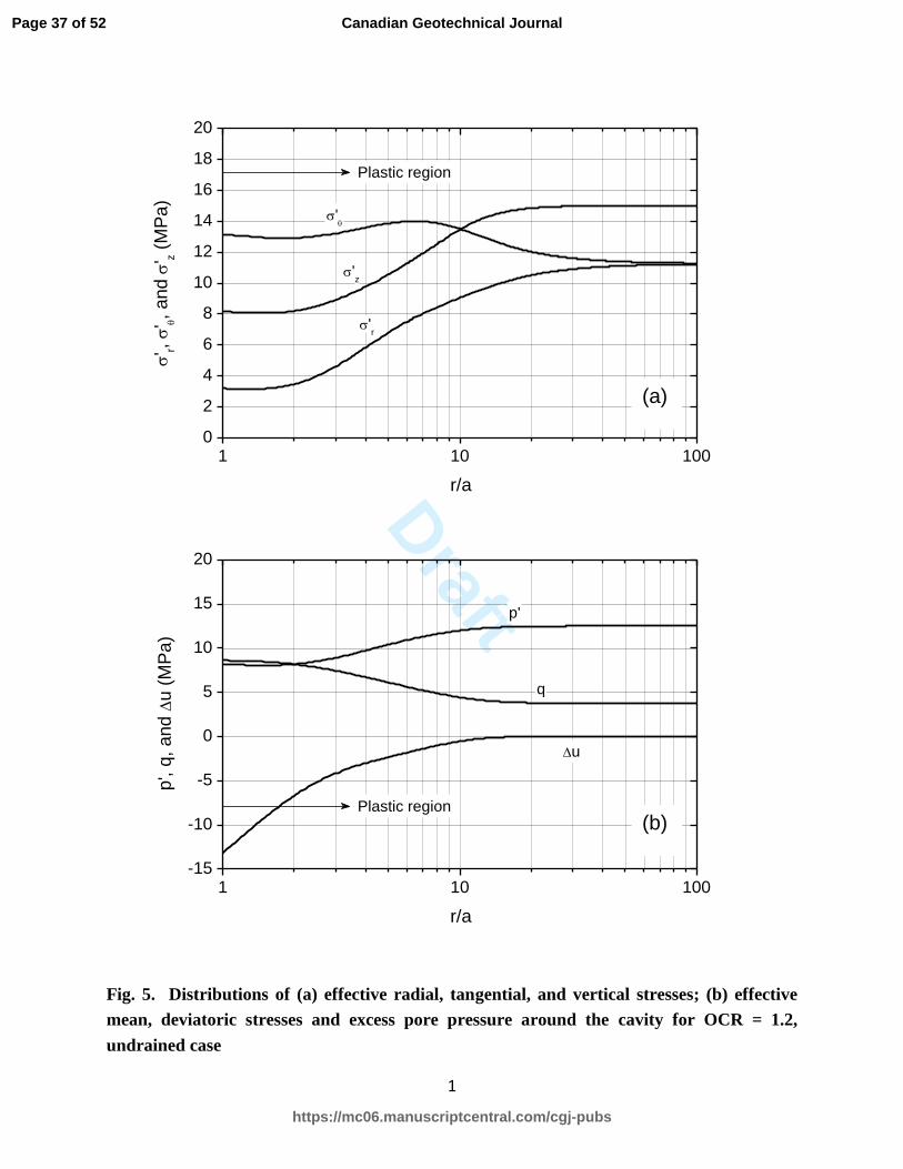
Figs. 4-7 show the distributions of �O, �P , and �Q and also of B′, D, and Δ� along the radial

distance corresponding to a reduced cavity pressure of �y = 0 for all the overconsolidation ratios

in the range from 1 to 5, where the radial axis has been normalized with respect to the current

contracted radius } and the results again presented for undrained case. It can be clearly observed

that for the case of �� = 1 (Fig. 4), all the radial, tangential, and vertical stresses as well as the

mean effective stress and deviatoric stress remain unchanged in the vicinity of the cavity Oy <

1.3, indicating the occurrence of critical state failure for the geomaterial of this range. However,

for larger values of �� = 1.2, 2, and 5, such an internal critical state zone vanishes and only

Page 19 of 52



Draft

20

the plastic zone may be expected outside the cavity. In fact, for given initial stresses (�O� =�P� = 11.25 MPa, �Q� = 15 MPa, and �� = 10 MPa), the lower the value of ��, the closer

the stress state at the cavity wall will approach the critical state.

Figs. 4-7 also clearly show that the negative excess pore pressure increases rapidly with

distance near the cavity. Especially, for normally consolidated geomaterial with �� = 1, Δ�

varies linearly with the logarithm of Oy in the critical state failure zone, an expected feature arising

from Eq. (44) for constant �O and �P . It is further interesting to note that the excess pore pressure

distribution is only slightly influenced by the varying level of overconsolidation, which differs

very much from the results in Chen and Abousleiman (2012) where significant impact of ��

has been observed on the pore pressure change for the Cam Clay model. Such a paradox occurs

because under the same reduced cavity pressure of �y = 0, the calculated excess pore pressure

shown in Figs. 4-7 for the four different values of �� actually corresponds to steadily

decreasing values of y<y = 1.40, 1.31, 1.18, and 1.10, respectively. Referring now to Fig. 3b, it

becomes obvious that the excess pore pressure developed indeed remains almost unchanged with

these y<y values. However, if the variation of ∆� is alternatively presented with respect to a

specified contracted cavity radius, say y<y = 1.2, one may foresee a considerable effect of ��

on the excess pore pressure distribution as similarly noted in Chen and Abousleiman (2012).

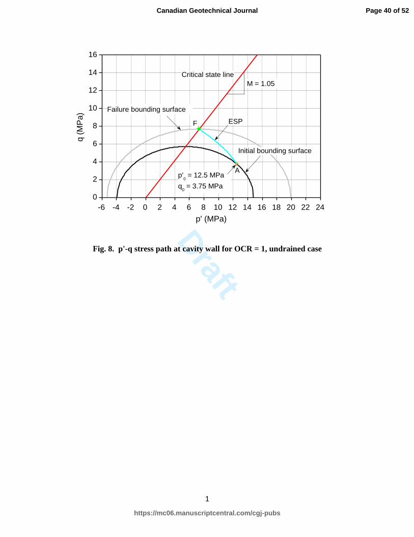
Figs. 8-11 further present the undrained effective stress path (ESP) followed in the B − D

plane for a material particle at the cavity wall. For �� = 1, recalling Eq. (39), the initial

bounding surface must pass through the initial stress point (Fig. 8). In this case the stress path

will start from B� = 12.5 MPa and D� = 3.75 MPa, continue to move upper-left and finally stop

at point � on the critical state line, which also lies on the failure bounding surface with B̅V =

Page 20 of 52



Draft

21

19.92 MPa (see Fig. 8). Since at point �, o = U and @ = 0 so '∗ = '(∗ while the latter is equal

to zero following Eq. (22) [n(U) = !I ], the actual plastic modulus '∗ must also vanish. This

explains why the stress path terminates on the critical state line and remains stationary there. For

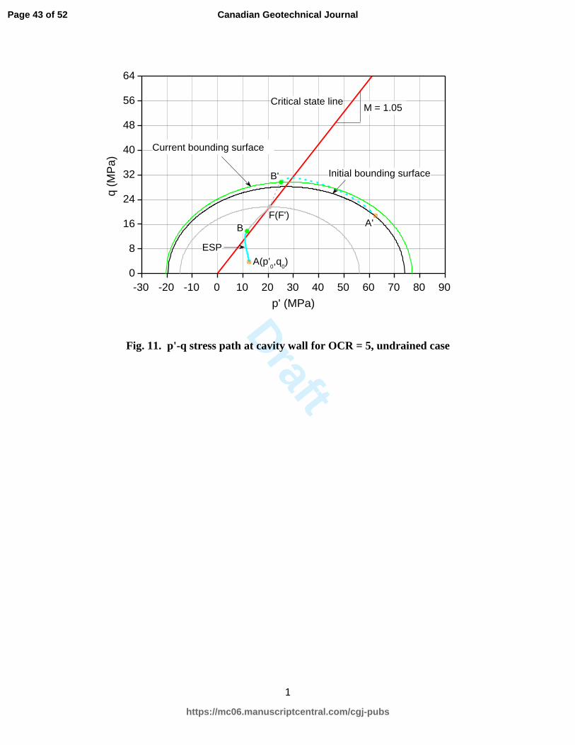
�� greater than 1, the initial stress point is always located within the initial bounding surface,

as shown in Figs. 9-11. Note that in the overconsolidation cases (�� > 1), the stress paths all

initially cross the critical state line parallel to the D axis, which makes a subtle difference from

the results when a regular plasticity model is used, e.g. the modified Cam Clay model (Chen

2012). As noted in Dafalias and Herrmann (1980), this is a property for any shape of bounding

surface which has � = 0 at o = U. In fact, at these cross points, @ > 0 and '∗ > '(∗ = 0, so

the material at this moment has not reached the failure state and therefore the stress paths may

bend over and continue to move towards the critical state line. To see this point more clearly, in

Fig. 11 for the case of �� = 5, the stress path is extended from point ª (�y = 0) to � which

corresponds to a sufficiently contracted cavity radius of yy< = 5. Also included in this figure is the

trajectory of the image stress (B̅, D�) on the expanding/contracting bounding surface, represented

by the curve «′ª′�′. As expected, the two points � and �′ coincide and both lie on the critical

state line again. This implies that the material has truly reached the failure state and that failure

can occur only if the loading surface merges with the bounding surface.

Note again that the use of the current version of bounding surface model excludes the

existence of a region of purely elastic response. However, if the value of the model parameter ℎ

is set extremely high in the computation, the plastic modulus '∗ [see Eq. (21)] will become so

large that the overall response of the material inside the bounding surface will be almost fully

elastic as in a classical yield surface formulation (Dafalias and Herrmann 1986). Fig. 12 shows

the profound effects of varying ℎ value on the support pressure versus cavity radius curve as well

Page 21 of 52



Draft

22

as on the B − D stress path for the case of �� = 5. In Fig. 12a, the cavity response becomes

stiffer (less deformable) as the plasticity parameter ℎ increases gradually from 30 to 300 and

then to 3000, but the �y − y<y curve, as anticipated, converges eventually to the limiting case of

classical yield surface plasticity when ℎ is sufficiently large equal to 30000. Such a feature is

even more clearly observed from Fig. 12b, where the stress path for ℎ = 30000 is nearly vertical

before it touches the initial bounding surface. This corresponds to a constant mean effective

stress B and provides a clear indication of purely elastic deformation of the material, which is

consistent with the finding in Chen and Abousleiman (2012) for the classical Cam Clay model.

One may thus conceive that the “real” material response shall be somewhere between the above-

mentioned two extremes of fully elasticity inside a classical yield surface and of always plasticity

inside a bounding surface, which can be suitably treated by the bounding surface model having

an elastic nucleus.

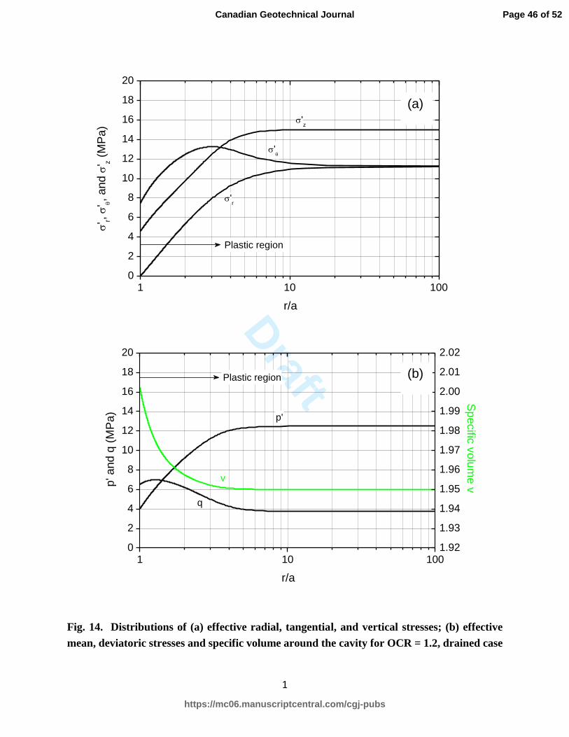
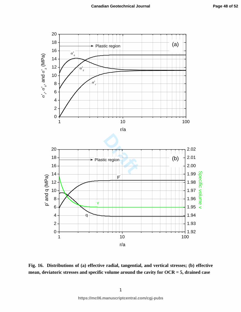
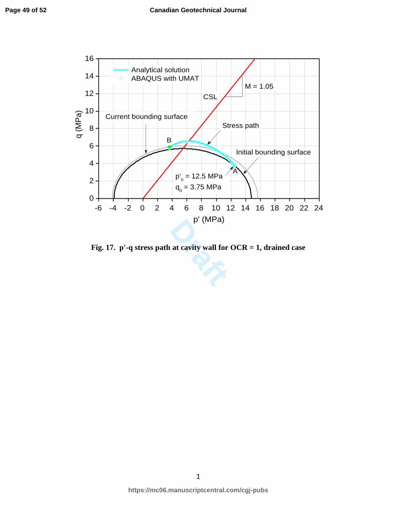
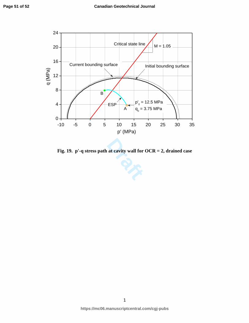
Figs. 13-20 show the calculation results of stresses and specific volume for the drained

situation, corresponding again to a zero effective cavity pressure which is defined as �y = �y −�� = 0 . Throughout the range of �� from 1 to 5 , it is observed that (Fig. 13-16) the

geomaterial undergoes dilation during the contraction process and the change in the specific

volume decreases with increasing ��. As regarding the B − D stress paths for different values

of ��, Figs. 17-20 illustrates that the material particles all first harden plastically from the wet

side of the critical state line (o < U ), the bounding surface expanding simultaneously to

accommodate the new stress state. After hitting the critical state line, the geomaterials start to

soften plastically in the dry side (o > U) and the bounding surface must decrease in size, the

stress paths eventually ending at point ª corresponding to �y = 0. One may expect that for

sufficiently small value of the cavity pressure, the stress path will be brought to the critical

Page 22 of 52



Draft

23

failure state again at lower values of B′ and D.

Fig. 17 also presents the Abaqus prediction of the B − D stress path at the cavity surface for

�� = 1, which has been conducted through the appropriate development and implementation

of the user subroutine (UMAT) for the bounding surface plasticity (Chen 2012) that is not

available in Abaqus finite element commercial program. It is clear that the numerical results are

in excellent agreement with the drained analytical solutions. This verifies the accuracy of the

proposed semi-analytical approach for the cavity contraction boundary value problem, and also

indicates the validity and reliability of the UMAT code written for the currently employed

bounding surface model.

Applications in tunnelling and wellbore drilling

This section examines the applications of the present semi-analytical solutions to the

modelling of tunnel excavation and wellbore drilling. For illustration purpose, only the undrained

condition will be considered and the emphasis will be given to the prediction of critical

(minimum) support pressure required to stabilize the tunnel and wellbore.

The critical support pressure �y,¬O could be defined in three different ways depending on the

stability criterion used for the tunnel/wellbore design (Yu 2000). The first one is based on the

elastic theory which assumes that the tunnel/wellbore will approach collapse condition once the

calculated elastic stress state anywhere around the cavity attains certain yielding criteria. With

reference to this criterion the critical support pressure therefore must correspond to the cavity

pressure for which the plastic deformation begins to take place at the tunnel/wellbore wall. The

other two criteria require the analysis of the tunnel/wellbore stability as an elastoplastic problem

(Charlez 1997; Yu 2000), as is elaborated in this paper. The tunnel and wellbore are regarded as

Page 23 of 52



Draft

24

unstable either when their surfaces reach the failure/critical state, or when their inward

displacements are too large to meet the allowable deformation requirement.

Recall now that the characteristic curves plotting the reduced support pressure as a function

of the contracted cavity radius, corresponding to the undrained condition, have been presented in

Fig. 3a. As a consequence, the critical support pressure �y,¬O can be directly obtained from these

curves for the first and third (allowable displacement) stability criteria. It is noteworthy that for

the bounding surface model, the material points around the cavity harden plastically immediately

after the cavity pressure drops below the in situ horizontal stress �� , so the critical support

pressure following the elastic analysis shall be �y,¬O = ��. The value of �y,¬O corresponding to

the second stability criterion (tunnel/wellbore wall reaching the critical state), however, needs to

be determined from the associated bounding surface critical state condition.

Table 2 compares the calculated results of �y,¬O based on the three stability criteria

mentioned above. The geomaterial parameters used in the analysis are the same as those listed in

Table 1, and two strain values of � = y<?yy< = 2% and 5% at the tunnel/wellbore surface have

been identified as controlling thresholds. It is found that a very large surface strain (contraction)

must have been mobilized before the tunnel/wellbore finally reach the critical state, and therefore

the critical state-based stability criterion is not controlling. Of course, which stability criterion,

i.e., tunnel/wellbore deformation exceeding the allowable limit or tunnel/wellbore stress reaching

the critical state, will control the design will be dependent on the actual soil/rock properties.

Table 2 also shows that the predicted �y,¬O in general decreases with the overconsolidation ratio,

which is reasonably expected as the higher the value of ��, the stiffer the geomaterials.

Page 24 of 52



Draft

25

Conclusions

This paper is devoted to developing the rigorous semi-analytical solutions for the drained

and undrained cavity contractions in geomaterials by using the bounding surface plasticity

model. One of the important features of the bounding surface model is that yielding could occur

as soon as loading commences in the stress space. Therefore, there is no purely elastic zone

existing outside the cavity during the contraction process. Extensive parametric studies show

that, for undrained problem, both the cavity pressure and the induced excess pore pressure

decrease significantly as the overconsolidation ratio of the geomaterials increases. The lower the

value of ��, the closer the stress state at the cavity wall will approach the critical state. In the

overconsolidation cases (�� > 1), it is found that the undrained stress paths all initially cross

the critical state line parallel to the D axis, then bend over and continue to move towards the

critical state line until they truly reach the failure state. For the drained case, the geomaterial

generally undergoes dilation during the cavity contraction and the change in the specific volume

decreases with increasing ��. The stress paths first head towards the critical state line from the

wet side, so the material hardens plastically accompanied by progressive expansion of the

bounding surface. After passing through the critical state line, the material however tends to

soften in the dry side and the bounding surface gradually decreases in size. The validity and

accuracy of the semi-analytical approach are justified by the finite element numerical modelling.

The proposed solutions are finally applied for the practical tunnelling and wellbore drilling

problems, to explore the critical support pressure that is required to maintain the tunnel/wellbore

stability.

Page 25 of 52



Draft

26

Acknowledgements

The work reported in this paper is partially supported by the PoroMechanics Institute

Industrial Consortium at the University of Oklahoma and the Oklahoma Center for the

Advancement of Science and Technology (Grant No. AR081-045). The valuable suggestions

from the anonymous reviewers are greatly appreciated.

References

Brown, E. T., Bray, J. W., Ladanyi, B., and Hoek, E. 1983. Ground response curves for rock

tunnels. Journal of Geotechnical Engineering Division, ASCE, 109(1): 15-39.

Carter, J. P. 1978. CAMFE: A computer program for the analysis of a cylindrical cavity

expansion in soil. Report CUED/C-Soils TR52, Department of Engineering, University of

Cambridge.

Carter, J. P., Booker, J. R., and Yeung, S. K. 1986. Cavity expansion in cohesive frictional soils.

Geotechnique, 36(3): 345-358.

Charlez, P. A. 1997. Rock mechanics Vol. 2: petroleum application. Editions Technip, Paris.

Charlez, P. A., and Roatesi, S. 1999. A fully analytical solution of the wellbore stability problem

under undrained conditions using a linearized Cam-Clay model. Oil & Gas Science and

Technology, 54(5): 551-563.

Chen, S. L. 2012. Analytical and numerical analyses of wellbore drilled in elastoplastic porous

formations. PhD thesis, The University of Oklahoma, USA.

Chen, S. L., and Abousleiman, N. Y. 2012. Exact undrained elastoplastic solution for cylindrical

cavity expansion in modified Cam Clay soil. Geotechnique, 62(5): 447-456.

Chen, S. L., and Abousleiman, N. Y. 2013. Exact drained solution for cylindrical cavity

expansion in modified Cam Clay soil. Geotechnique, 63(6): 510-517.

Page 26 of 52



Draft

27

Collins, I. F., and Stimpson, J. R. 1994. Similarity solutions for drained and undrained cavity

expansions in soils. Geotechnique, 44(1): 21-34.

Dafalias, Y. F., and Herrmann, L. R. 1980. A bounding surface soil plasticity model. In

Proceedings of the International Symposium on Soils under Cyclic and Transient Loading.

Edited by Pande, G. N., and Zienkiewicz, O. Z. pp. 335-345.

Dafalias, Y. F., and Herrmann, L. R. 1982. Bounding surface formulation of soil plasticity. In

Soil Mechanics-Transient and Cyclic Loads. Edited by Pande, G. N., and Zienkiewicz, O. Z.

pp. 253-282.

Dafalias, Y. F., and Herrmann, L. R. 1986. Bounding surface plasticity II: Application to

isotropic cohesive soils. Journal of Engineering Mechanics, ASCE, 112(12): 1263-1291.

Dafalias, Y. F., and Popov, E. P. 1975. A model of nonlinearly hardening materials for complex

loadings. Acta Mechanica, 21: 173-192.

Dafalias, Y. F., and Popov, E. P. 1976. Plastic internal variables formalism of cyclic plasticity.

Journal of Applied Mechanics ASME, 98(4): 645-650.

Gibson, R. E., and Anderson, W. F. 1961. In situ measurement of soil properties with the

pressuremeter. Civil Engineering and Public Works Review, 56(658): 615-618.

Graziani, A., and Ribacchi, R. 1993. Critical conditions for a tunnel in a strain softening rock. In

Assessment and Prevention of Failure Phenomena in Rock Engineering. Edited by

Pasamehmetoglu, A. G., Kawamoto, T., Whittaker, B. N., and Aydan, O. pp. 199-204.

Kaliakin, V. N., Dafalias, Y. F., and Herrmann, L. R. 1987. Time dependent bounding surface

model for isotropic cohesive soils, Note for a short course. Tucson, Arizona.

Kaliakin, V. N., and Dafalias, Y. F. 1989. Simplifications to the Bounding Surface Model for

Cohesive Soils. International Journal for Numerical and Analytical Methods in

Geomechanics, 13(1): 91-100.

Page 27 of 52



Draft

28

Manzari, M. T., and Nour, M. A. 1997. On implicit integration of bounding surface plasticity

models. Computers & Structures, 63(3): 385-395.

Papanastasiou, P., and Durban, D. 1997. Elastoplastic analysis of cylindrical cavity problems in

geomaterials. International Journal for Numerical and Analytical Methods in Geomechanics,

21(2): 133-149.

Potts, D. M., and Zdravkovic, L. 1999. Finite element analysis in geotechnical engineering:

theory. Thomas Telford Ltd.

Randolph, M. F., Carter, J. P., and Wroth, C. P. 1979. Driven piles in clay-the effects of

installation and subsequent consolidation. Geotechnique, 29(4): 361-393.

Reed, M. B. 1988. The influence of out-of-plane stress on a plane strain problem in rock

mechanics. International Journal for Numerical and Analytical Methods in Geomechanics,

12(2): 173-181.

Russell, A. R., and Khalili, N. 2006. On the problem of cavity expansion in unsaturated soils.

Computational Mechanics, 37(4): 311-330.

Salgado, R., and Randolph, M. F. 2001. Analysis of cavity expansion in sand. International

Journal of Geomechanics, ASCE, 1(2): 175-192.

Vesic, A. C. 1972. Expansion of cavities in infinite soil mass. Journal of the Soil Mechanics and

Foundations Division, ASCE, 98(SM3): 265-290.

Wood, D. M. 1990. Soil behaviour and critical state soil mechanics. Cambridge University Press,

Cambridge, UK.

Yu, H. S. 1990. Cavity expansion theory and its application to the analysis of pressuremeters.

PhD thesis, University of Oxford, UK.

Yu, H. S. 2000. Cavity expansion methods in geomechancis. Kluwer Academic Publishers,

Dordrecht.

Page 28 of 52



Draft

29

Yu, H. S., and Rowe, R. K. 1999. Plasticity solutions for soil behavior around contracting

cavities and tunnels. International Journal for Numerical and Analytical Methods in

Geomechanics, 23(12): 1245-1279.

Captions of table and figures

Table 1. Parameters used in example analyses with bounding surface model

Table 2. Predicted �y,¬O using three different stability criteria

Fig. 1. Schematic illustration of bounding surface and radial mapping rule in general stress (σ'ij)

space and p'-q space

Fig. 2. Geometry of cavity boundary value problem

Fig. 3. Variations of (a) cavity pressure; (b) excess pore pressure at cavity wall with

normalized cavity radius for undrained case

Fig. 4. Distributions of (a) effective radial, tangential, and vertical stresses; (b) effective mean,

deviatoric stresses and excess pore pressure around the cavity for OCR = 1, undrained

case


deviatoric stresses and excess pore pressure around the cavity for OCR = 1.2, undrained

case



case

Page 29 of 52



Draft

30



case

Fig. 8. p'-q stress path at cavity wall for OCR = 1, undrained case

Fig. 9. p'-q stress path at cavity wall for OCR = 1.2, undrained case



Fig. 12. Influences of plasticity parameter h on (a) support pressure versus cavity radius curve;

(b) p’-q effective stress path with zero support pressure (σa = 0), undrained case and

OCR = 5


deviatoric stresses and specific volume around the cavity for OCR = 1, drained case


deviatoric stresses and specific volume around the cavity for OCR = 1.2, drained case





Fig. 17. p'-q stress path at cavity wall for OCR = 1, drained case

Fig. 18. p'-q stress path at cavity wall for OCR = 1.2, drained case



Page 30 of 52



Draft

1

Table 1. Parameters used in example analyses with bounding surface model

�� = ��

� = 11.25 MPa, �� = 15 MPa, �� = 10 MPa, ��

� = 12.5 MPa, and �� = 3.75 MPa

� � � � � �� ℎ �̅�,�

� (MPa)

"#� = 1 1.2 2 5

2.72 1.05 0.14 0.05 0.15 0.95 0.2 30 14.80 17.76 29.60 74.00

Page 31 of 52



Draft

1

Table 2. Predicted ��,�� using three different stability criteria

OCR Elastic

analysis

Allowable deformation

� = 2%

Allowable deformation

� = 5%

Cavity surface

reaches critical state

1 21.25 MPa

(� = 0) 13.34 MPa 9.50 MPa

2.96 MPa

(� = 18%)

1.2 21.25 MPa

(� = 0) 13.12 MPa 9.00 MPa

0.55 MPa (� = 25%)

2 21.25 MPa

(� = 0) 12.48 MPa 7.58 MPa

-7.46 MPa

(� = 35%)

5 21.25 MPa

(� = 0) 11.32 MPa 5.10 MPa

-27.62 MPa (� = 53%)

Page 32 of 52



Draft

1

Fig. 1. Schematic illustration of bounding surface and radial mapping rule in general stress

(σ'ij) space and p'-q space

o p̅'C

(p', q)

p'A

M Critical state line

np

nq nij

p̅'C /R

nij

δ

(p̅', q̅)

or F̅(p̅', q̅, ep) = 0

δ0

Bounding surface

or

(q) σ′ij

(p’) σ′ij

σ̅′ij

σ′ij dσ′ij

F̅(σ̅′ij, ep) = 0

Loading surface

F(σ′ij) = 0

Page 33 of 52



Draft

1

Fig. 2. Geometry of cavity boundary value problem

a

Plastic region

σh σh

σh

σa

σv

rx

a0 rx0 r

Failure

u0

σh

Page 34 of 52



Draft

1

Fig. 3. Variations of (a) cavity pressure; (b) excess pore pressure at cavity wall with

normalized cavity radius for undrained case

1.00 1.05 1.10 1.15 1.20 1.25 1.30 1.35 1.40 1.45 1.50-20

-10

0

10

20

30

5

2

1.2

Ca

vity p

ressu

re

a (

MP

a)

a0/a

OCR = 1

1.00 1.05 1.10 1.15 1.20 1.25 1.30 1.35 1.40 1.45 1.50-40

-35

-30

-25

-20

-15

-10

-5

0

5

2

1.2

Exce

ss p

ore

pre

ssu

re

u (

MP

a)

a0/a

OCR = 1

(a)

(b)

Page 35 of 52



Draft

1

Fig. 4. Distributions of (a) effective radial, tangential, and vertical stresses; (b) effective

mean, deviatoric stresses and excess pore pressure around the cavity for OCR = 1, undrained

case

1 10 1000

2

4

6

8

10

12

14

16

18

20

'r

'z

Plastic region

'

' r, ' ,

an

d

' z (

MP

a)

r/a

Critical state region

1 10 100-15

-10

-5

0

5

10

15

20

q

u

p'

p', q

, and

u (

MP

a)

r/a

Critical state region

Plastic region

(a)

(b)

Page 36 of 52



Draft

1


mean, deviatoric stresses and excess pore pressure around the cavity for OCR = 1.2,

undrained case

1 10 1000

2

4

6

8

10

12

14

16

18

20

'r

'z

Plastic region

'

' r, ' ,

an

d

' z (

MP

a)

r/a

1 10 100-15

-10

-5

0

5

10

15

20

q

u

p'

p', q

, a

nd

u

(M

Pa

)

r/a

Plastic region

(a)

(b)

Page 37 of 52



Draft

1



case

1 10 1000

2

4

6

8

10

12

14

16

18

20

'r

'z

Plastic region

'

' r, ' ,

an

d

' z (

MP

a)

r/a

1 10 100-15

-10

-5

0

5

10

15

20

q

u

p'

p', q

, a

nd

u

(M

Pa

)

r/a

Plastic region

(a)

(b)

Page 38 of 52



Draft

1



case

1 10 1000

2

4

6

8

10

12

14

16

18

20

'r

'z

Plastic region

'

' r, ' ,

an

d

' z (

MP

a)

r/a

1 10 100-15

-10

-5

0

5

10

15

20

q

u

p'

p', q

, a

nd

u

(M

Pa

)

r/a

Plastic region

(a)

(b)

Page 39 of 52



Draft

1


-6 -4 -2 0 2 4 6 8 10 12 14 16 18 20 22 24

0

2

4

6

8

10

12

14

16

A

Failure bounding surface

p'0 = 12.5 MPa

q0 = 3.75 MPa

ESP

M = 1.05

Critical state line

p' (MPa)

q (

MP

a)

Initial bounding surface

F

Page 40 of 52



Draft

1

Fig. 9. p'-q stress path at cavity wall for OCR = 1.2, undrained case

-6 -4 -2 0 2 4 6 8 10 12 14 16 18 20 22 24

0

2

4

6

8

10

12

14

16

B

A

Current bounding surface

p'0 = 12.5 MPa

q0 = 3.75 MPa

ESP

M = 1.05Critical state line

p' (MPa)

q (

MP

a)


Page 41 of 52



Draft

1


-10 -5 0 5 10 15 20 25 30 35

0

4

8

12

16

20

24

B

A


p'0 = 12.5 MPa

q0 = 3.75 MPa

ESP


p' (MPa)

q (

MP

a) Initial bounding surface

Page 42 of 52



Draft

1


-30 -20 -10 0 10 20 30 40 50 60 70 80 90

0

8

16

24

32

40

48

56

64

F(F')

B'

BA'

A(p'0,q

0)


ESP


p' (MPa)

q (

MP

a)


Page 43 of 52



Draft

1

Fig. 12. Influences of plasticity parameter h on (a) support pressure versus cavity radius

curve; (b) p’-q effective stress path with zero support pressure (σa = 0), undrained case and

OCR = 5

1.00 1.05 1.10 1.15 1.20 1.25 1.30 1.35 1.40 1.45 1.50-50

-40

-30

-20

-10

0

10

20

30

h = 30

300

3000

Ca

vity p

ressu

re

a (

MP

a)

a0/a

30000

-30 -20 -10 0 10 20 30 40 50 60 70 80 90

0

8

16

24

32

40

48

56

64

h = 300

A(p'0,q

0)

h = 30000

h = 30


p' (MPa)

q (

MP

a)


(a)

(b)

Page 44 of 52



Draft

1


mean, deviatoric stresses and specific volume around the cavity for OCR = 1, drained case

1 10 1000

2

4

6

8

10

12

14

16

18

20

'r

'z

Plastic region

'

' r, ' ,

an

d

' z (

MP

a)

r/a

1 10 1000

2

4

6

8

10

12

14

16

18

20

Sp

ecific

vo

lum

e v

v

q

p

' a

nd

q (

MP

a)

r/a

p'

Plastic region

1.92

1.93

1.94

1.95

1.96

1.97

1.98

1.99

2.00

2.01

2.02

(a)

(b)

Page 45 of 52



Draft

1


mean, deviatoric stresses and specific volume around the cavity for OCR = 1.2, drained case

1 10 1000

2

4

6

8

10

12

14

16

18

20

'r

'z

Plastic region

'

' r, ' ,

an

d

' z (

MP

a)

r/a

1 10 1000

2

4

6

8

10

12

14

16

18

20

Sp

ecific

vo

lum

e v

v

q

p

' a

nd

q (

MP

a)

r/a

p'

Plastic region

1.92

1.93

1.94

1.95

1.96

1.97

1.98

1.99

2.00

2.01

2.02

(a)

(b)

Page 46 of 52



Draft

1



1 10 1000

2

4

6

8

10

12

14

16

18

20

'r

'z

Plastic region

'

' r, ' ,

an

d

' z (

MP

a)

r/a

1 10 1000

2

4

6

8

10

12

14

16

18

20

Sp

ecific

vo

lum

e vv

q

p

' an

d q

(M

Pa

)

r/a

p'

Plastic region

1.92

1.93

1.94

1.95

1.96

1.97

1.98

1.99

2.00

2.01

2.02

(a)

(b)

Page 47 of 52



Draft

1



1 10 1000

2

4

6

8

10

12

14

16

18

20

'r

'z

Plastic region

'

' r, ' ,

an

d

' z (

MP

a)

r/a

1 10 1000

2

4

6

8

10

12

14

16

18

20

Sp

ecific

vo

lum

e vv

q

p

' a

nd

q (

MP

a)

r/a

p'

Plastic region

1.92

1.93

1.94

1.95

1.96

1.97

1.98

1.99

2.00

2.01

2.02

(a)

(b)

Page 48 of 52



Draft

1


-6 -4 -2 0 2 4 6 8 10 12 14 16 18 20 22 24

0

2

4

6

8

10

12

14

16

CSL

Stress path

Analytical solution

ABAQUS with UMAT

A


p'0 = 12.5 MPa

q0 = 3.75 MPa

M = 1.05

p' (MPa)

q (

MP

a)


B

Page 49 of 52



Draft

1

Fig. 18. p'-q stress path at cavity wall for OCR = 1.2, drained case

-6 -4 -2 0 2 4 6 8 10 12 14 16 18 20 22 24

0

2

4

6

8

10

12

14

16

A


p'0 = 12.5 MPa

q0 = 3.75 MPa

ESP

M = 1.05

Critical state line

p' (MPa)

q (

MP

a)


B

Page 50 of 52



Draft

1


-10 -5 0 5 10 15 20 25 30 35

0

4

8

12

16

20

24

B

A


p'0 = 12.5 MPa

q0 = 3.75 MPa

ESP


p' (MPa)

q (

MP


Page 51 of 52



Draft

1


-30 -20 -10 0 10 20 30 40 50 60 70 80 90

0

8

16

24

32

40

48

56

64

B

A


p'0 = 12.5 MPa

q0 = 3.75 MPa

ESP


p' (MPa)

q (

MP


Page 52 of 52



environmental engineering solutions; stress path ... · pdf filesolution for the wellbore...

Documents