environmental data mining and modeling based on machine learning algorithms and geostatistics

Environmental Modelling & Software 19 (2004) 845–855www.elsevier.com/locate/envsoft

Environmental data mining and modeling based on machinelearning algorithms and geostatistics

M. Kanevskia,b, R. Parkinc,∗, A. Pozdnukhova,c,d, V. Timonin c, M. Maignanb,V. Demyanovc, S. Canue

a IDIAP Dalle Molle Institute for Perceptual Artificial Intelligence, Simplon 4, 1920 Martigny, Switzerlandb Lausanne University, Lausanne, Switzerland

c IBRAE, Nuclear Safety Institute, Russian Academy of Sciences, Environmental Modelling and System Analysis Laboratory, 52 B, Tulskaya,Moscow 113191, Russia

d Physics Department, Moscow State University, Math. Division, Moscow, Russiae INSA, Rouen, France

Received 30 September 2002; received in revised form 13 January 2003; accepted 5 March 2003

Abstract

The paper presents some contemporary approaches to spatial environmental data analysis. The main topics are concentrated onthe decision-oriented problems of environmental spatial data mining and modeling: valorization and representativity of data withthe help of exploratory data analysis, spatial predictions, probabilistic and risk mapping, development and application of conditionalstochastic simulation models. The innovative part of the paper presents integrated/hybrid model—machine learning (ML) residualssequential simulations—MLRSS. The models are based on multilayer perceptron and support vector regression ML algorithms usedfor modeling long-range spatial trends and sequential simulations of the residuals. ML algorithms deliver non-linear solution forthe spatial non-stationary problems, which are difficult for geostatistical approach. Geostatistical tools (variography) are used tocharacterize performance of ML algorithms, by analyzing quality and quantity of the spatially structured information extracted fromdata with ML algorithms. Sequential simulations provide efficient assessment of uncertainty and spatial variability. Case study fromthe Chernobyl fallouts illustrates the performance of the proposed model. It is shown that probability mapping, provided by thecombination of ML data driven and geostatistical model based approaches, can be efficiently used in decision-making process. 2003 Elsevier Ltd. All rights reserved.

Keywords: Environmental data mining and assimilation; Geostatistics; Machine learning; Stochastic simulation; Radioactive pollution

1. Introduction

Environmental data feature complex spatial pattern atdifferent scales due to combination of several spatialphenomena or various influencing factors of differentorigins. In some cases, the original observations aretaken with significant measurement errors and may con-tain significant uncertainty as well as a number of out-liers. Non-linear spatial trends corresponding to large-scale processes complicate geostatistical modeling aslong as stationary models (e.g. ordinary kriging) are con-

∗ Corresponding author. Tel.:+7-095-955-2231; fax:+7-095-958-1151.

E-mail addresses: [email protected] (M. Kanevski); [email protected] (R. Parkin); [email protected] (A. Pozdnukhov).

1364-8152/$ - see front matter 2003 Elsevier Ltd. All rights reserved.doi:10.1016/j.envsoft.2003.03.004

cerned. Trend removal is also necessary for comprehen-sive spatial correlation analysis and modeling(variography). Variogram modeling for such data andusing common geostatistical approaches will result inincorrect results. In the presence of trends, the data canbe decomposed into two parts:

Z(x) � M(x) � e(x) (1)

where M(x) represents large-scale deterministic spatialvariations (trends), ande(x) represents small-scale spa-tial stochastic variations. Contemporary geostatisticsoffers several possible approaches to handle spatialtrends (spatial non-stationarity): universal kriging(implying a polynomial trend model), residual kriging,moving window regression residual kriging (seeCressie,1991; Deutsch and Journel, 1998; Dowd, 1994; Neuman

846 M. Kanevski et al. / Environmental Modelling & Software 19 (2004) 845–855

and Jacobson, 1984; Gambolati and Galeati, 1987; Hass,1996). All these approaches imply a certain formulabased trend model, which is not necessarily in a goodagreement with the data. An alternative way for trendmodeling is to use a data-driven approach, which reliesonly on data. One of such approaches was developed bypartitioning heterogeneous study area into some smallerhomogeneous subareas and analyzing the spatial struc-ture within them separately (Pelissier and Goreaud,2001).

In the present paper, we propose a newly developedmodel—machine learning residuals sequential Gaussiansimulations (MLRSGS) as an extension of the ideaspresented by Kanevsky et al. (1996b) and Demyanov etal. (2000). In these papers, a hybrid model—neural net-work residuals kriging (NNRK)—was first introducedand then extended for use in a combination with differentgeostatistical models. The basic idea is to use feedfor-ward neural network (FFNN), which is a well-knownglobal universal approximator to model large-scale non-linear trends, and then to apply geostatisticalestimators/simulators for the residuals. Machine learningalgorithms unite a wide family of data-driven models.Here, we will focus on two of them: multilayer per-ceptron (MLP) and support vector regression (SVR).Another type of hybrid models (expert systems) wasdeveloped by using geographical information systemsand modeling integrated into a decision support systemfor environmental and technological risk assessment andmanagement (see Fedra and Winkelbauer, 1999).

One of the principal advantages of machine learningalgorithms is their ability to discover patterns in data,which exhibit significant unpredictable non-linearity.Being a data-driven approach (“black-box” models), MLdepends only on the quality of data and the architectureof model, particularly for MLP—number of hidden neu-rons, activation functions types of connections. ML cancapture spatial peculiarities of the pattern at differentscales describing both linear and non-linear effects. Per-formance of MLA is based on solid theoretical foun-dations, which were considered by Bishop (1995), Hay-kin (1999) and Vapnik (1998).

Stochastic simulation is an intensively developed andused approach to provide uncertainty and risk assess-ment for spatial and spatio-temporal problems. Stochas-tic simulation models are preferable over estimators asthey are able to provide a joint probabilistic distributionsrather than a single value estimates. Sequential Gaussiansimulation (SGS) is one of the widely used methods thatis able to handle highly variable data but still is sensitiveto trend, thus formally requires to some extent spatialstationarity assumed. SGSs are based on modeling ofspatial correlation structures—variography.

A mixture of ML data driven and geostatistical modelbased approaches is also attractive for decision-makingprocess because of their interpretability.

The real case study on soil pollution from the Cherno-byl fallout illustrates the application of the proposedmodel. The accident at Chernobyl nuclear power plantcaused large-scale contamination of environment byradiologically important radionuclides. Large-scaleconsequences of the Chernobyl fallout were consideredin the past decade and one of the comprehensive map-ping work was presented in De Cort and Tsaturov(1996). Geostatistical analysis and prediction modelingof radioactive soil contamination data was presented inKanevsky et al. (1996a).

2. Machine learning residual Gaussian simulations

2.1. Methodology of ML residual Gaussiansimulations

The basic idea is to use ML to develop a non-para-metric, robust model to extract large-scale non-linearstructures from data (detrending) and then to use geosta-tistical models to simulate the residuals at local scales.In brief, the MLRSGS algorithm follows the steps givenbelow (extended after Kanevsky et al., 1996b):

1. Data preprocessing and exploratory analysis: in gen-eral, split data into training, testing and validationsets, checking for outliers, exploratory data analysis,estimations and modeling of spatial correlation—experimental and theoretical variography. Trainingset is used for the ML algorithms training, validationset is used to tune hyperparameters (e.g. number ofhidden neurons) while testing set is applied to assessMLA generalization ability.

2. Training and testing of ML algorithm. In the presentpaper, MLP and SVR are used. They are well-knownfunction approximators and are described brieflybelow.

3. Accuracy test—comprehensive analysis of theresiduals provides the ML residuals at the trainingpoints (measured–estimated) which are the base forfurther analysis. Two further cases are possible:

� the residuals are not correlated with the measurementscorrelated (both 1D and 2D), which means that MLAhas modeled all spatial structures presented in theraw data;

� the residuals show some correlation with the samples,then further analysis should be performed on theresiduals to model this correlation.

4. ML residuals are explored using variography. Theremaining spatial correlation presents short-rangecorrelation structures, once long-range correlation(trend) in the whole area was modeled by MLA.

5. Normal score transformation (non-linear transform-ation from raw data to Nscore values, distributed

847M. Kanevski et al. / Environmental Modelling & Software 19 (2004) 845–855

N(0,1) is performed to prepare data for further Gaus-sian simulations. Nscore variogram model describingspatial correlations of Nscore values is built. SGS isthen applied to the MLA residuals and stochastic real-izations are generated using the training dataset.

The idea of stochastic simulation is to develop a spa-tial Monte Carlo model that will be able to generatemany, in some sense equally probable, realizations of arandom function (in general, described by a joint prob-ability density function). Any realization of the randomfunction is called an unconditional simulation. Realiza-tions that honor the data are called conditional simula-tions. Basically, the simulations try to reproduce the first(univariate global distribution) and the second(variogram) moments. The similarities and dissimi-larities between the realizations describe spatial varia-bility and uncertainty. The simulations bring valuableinformation on the decision-oriented mapping of pol-lution. Postprocessing of the simulated realizations pro-vides probabilistic maps: maps of probabilities of thefunction value to be above/below some predefineddecision levels. Gaussian random function models arewidely used in statistics and simulations due to their ana-lytical simplicity, they are well understood and are limitdistributions of many theoretical results. SGS algorithmused in this work was described in detail in Deutsch andJournel (1998).

6. Simulated values of the residuals appear after backnormal score transformation. Final ML residualsimulations value is a sum of ML estimate andSGS realization.

2.2. Description of multilayer perceptron model

MLP is a type of artificial neural network with a spe-cific structure and training procedure described inBishop (1995) and Haykin (1999).

The key component of MLP is the formal neuron,which sums the inputs, and performs a non-linear trans-form via the activation function f (Fig. 1). The activation

Fig. 1. Formal neuron.

function (or non-linear transformer) can be any continu-ous, bounded and non-decreasing function. Exponentialsigmoid or hypertangent are commonly used in practice.The weights W(w0, …, wn) are adaptive parameterswhich are optimized by minimizing the following quad-ratic cost function:

MSE �1N�N

i � 1

(ti�oi)2 (2)

where MSE is the mean square error, N is the numberof samples, oi is the net output (prediction) and ti is thereal function desired value. Backpropagation error algor-ithm is applied to calculate gradient of MSE on adaptiveweight, ∂E /∂W. Various optimization algorithms, whichemploy backpropagation, can be used, such as the conju-gate gradient descend method, second-order pseudo-Newton Levenberg-Marquardt method, or the resilientpropagation method.

In a standard MLP, the neurons are arranged in input,hidden and output layers. The values of the exploratoryvariables (X and Y co-ordinates) are exposed to the inputlayer, the output layer produces and compares the targetestimate of the function value (137Cs concentration), hid-den layers (one or two) allow(s) to handle non-linearity(Fig. 2). The number of neurons in the hidden layers canvary and is the subject to the optimum configuration. Aslong as the aim of MLP in the present work is to extracta large-scale trend, as few hidden neurons as possiblewere chosen to extract non-linear trends. Furtherincrease of the number of hidden neurons leads toextracting more detailed local peculiarities and evennoise from the pattern: choosing too many hidden neu-rons will lead to over-fitting (or over-learning) whenMLP loses its ability to generalize the information fromthe samples. On the other hand, using too few hiddenneurons does not provide explicit extraction of the trend;hence some large-scale correlations will remain in theresiduals restricting further procedure. Thus, geostatist-ical variogram analysis becomes the key tool to controlthe MLP performance for trend extraction.

Fig. 2. Multilayer perceptron.


2.3. Description of support vector regression model

SVR is a recent development of the statistical learningtheory (SLT) (Vapnik, 1998). It is based on structuralrisk minimization and seems to be promising approachfor spatial data analysis and processing (see Scholkopfand Smola, 1998; Gilardi and Bengio, 2000; Kanevskiet al., 2001). There are several attractive properties ofthe SVR: robustness of the solution, sparseness of theregression, automatic control of the solutions com-plexity, good generalization performance (Vapnik,1998). In general, by tuning SVR hyper-parameters, itis possible to cover a wide range of spatial regressionfunctions from over-fitting to over-smoothing (Kanevskiet al., 2001).

First, we state a general problem of regression esti-mation as it is presented in the scope of SLT. Let{(x1,y1),…(xN,yN)} be a set of observations generatedfrom an unknown probability distribution P(x, y) withxi�Rn, yi�R, and F = {f�Rn→R} a class of functions.The task is to find a function f from the given class offunctions that minimizes a risk functional:

R[f] � �Q(y�f(x),x)dP(x,y) (3)

where Q is a loss function indicating how the differencebetween the measurement value and the model’s predic-tion is penalized.

As P(x, y) is unknown, one can compute an empiri-cal risk:

Remp �1N�N

i � 1

Q(yi�f(xi),xi) (4)

When it is only known that noise-generating distri-bution is symmetric, the use of linear loss function ispreferable, and results in a model from robust regressionfamily. For simplicity, we also assume loss to be thesame for all spatial locations.

The Support vector regression model is based on anew type of loss functions, the so-called e-insensitiveloss functions. Symmetric linear e-insensitive loss isdefined as:

Q(y�f(x),x) � �|y�f(x)|�e, if |y�f(x)| � e

0, otherwise(5)

The asymmetrical loss function can be used in appli-cations where underestimations and overestimations arenot equivalent.

Let us start from the estimation of regression functionin a class of linear functions F = {f(x)�f(x) = (w,x) +b}. Support vector regression is based on the structuralrisk minimization principle, which results in penalizationof the model complexity simultaneously with keepingsmall empirical risk (training error). The complexity of

linear functions can be controlled by the term ||w||2, seeEq. (6) (Vapnik, 1998). Also, we have to minimize theempirical risk (training error). With selected symmetricallinear e-insensitive loss, empirical risk minimization isequivalent to adding the slack variables xi,x∗i into thefunctional with the linear constraints (7). Introducing thetrade-off constant C, we arrive at the following optimiz-ation problem:

minimize12

��w��2 � C�Ni � 1

(xi � x∗i ) (6)

subject to �f(xi)�yi�e�xi

�f(xi) � yi�e�x∗ixi,x∗i �0, for i � 1,…,N

(7)

The slack variables xi,x∗i measure the distancebetween the observation and the ε tube. The distancebetween the observation and the e and xi,x∗i is illustratedby the following example: imagine you have a great con-fidence in your measurement process, but the varianceof the measured phenomena is large. In this case, e hasto be chosen a priori very small while the slack variablesxi,x∗i are optimized and thus can be large. Rememberthat inside the ε tube ([f(x)�e,f(x) + e]) loss functionis zero.

Note that by introducing the couple (xi,x∗i ), the prob-lem now has 2n unknown variables. But these variablesare linked since one of the two values is a necessaryequal to zero. Either the slack is positive (x∗i = 0) ornegative (xi = 0). Thus, yi�[f(xi)�e�xi,f(xi) + e + x∗i ].

A classical way to reformulate the constraint basedminimization problem is to look for the saddle point ofLagrangian L:

L(w,x,x∗a) �12��w��2 � C�N

i � 1

(xi � x∗i )��Ni � 1

ai(yi

�f(xi) � e � xi)��Ni � 1

a∗i (f(xi)�yi � e � x∗i ) (8)

��Ni � 1

(hixi � h∗i x∗i )

where ai,a∗i ,hi,h∗

i are Lagrange multipliers associatedwith the constraints; ai,a∗

i can be roughly interpreted asa measure of the influence of the constraints on the sol-ution. A solution with ai = a∗

i = 0 can be interpreted as“ the corresponding data point has no influence on thissolution” . Other points with non-zero ai or a∗

i are the“support vectors (SVs)” of the problem.

The dual formulation of the optimization problem issolved in practice:


maximise �12�

N

i � 1

�Nj � 1

(a∗i �ai)(a∗

j �aj)(xi·xj) (9)

�e�Ni � 1

(a∗i � ai) � �N

i � 1

yi(a∗i �ai)

subject to ��Ni � 1

(a∗i �ai) � 0

0�a∗i ,ai�C, for i � 1,…,N

This is a quadratic programming (QP) problem, hencehas an unique solution. It can be solved numerically bya number of methods. After we get the values ai anda∗

i , we can compute b from the constraints of the pri-mary problem (7) and make predictions:

f(x) � �Ni � 1

(a∗i �ai)(xi·x) � b (10)

Note that both the solution (10) and the optimizationproblem (9) are written in the terms of dot products.Hence, we can use a so-called “kernel trick” to achievenon-linear regression model. We substitute the dot pro-ducts (xi,xj) with a suitable function{K�L2(Rn)�L2(Rn),K�(Rn�Rn)→R}. If the kernel func-tion satisfies the Mercer’s conditions:

��K(x�,x�)g(x�)g(x�)dx�dx� � 0 (11)

for any g(x)�L2(Rn), then it can be expanded in a uni-formly converging series

K(x�,x�) � �j

ljj(x�)j(x�) (12)

where {li,j(.)} is an eigensystem of K. We may regardj(x) as some j-th feature of vector x, then kernel K isa dot product in some feature space. As (11) determinespositively defined kernels, the substitution of K insteadof dot products in (9) results in a still convex QP prob-lem:

maximise �12�

N

i � 1

�Nj � 1

(a∗i �ai)(a∗

j �aj)K(xi,xj) (13)

�e�Ni � 1

(a∗i � ai) � �N

i � 1

yi(a∗i �ai)

subject to ��Ni � 1

(a∗i �ai) � 0

0�a∗i ,ai�C, for i � 1,…N

and the prediction is a non-linear regression function:

f(x) � �Ni � 1

(a∗i �ai)K(xi,x) � b (14)

3. Case study

Radioactive soil contamination caused by the Cherno-byl fallout features anisotropic highly variable and spottyspatial pattern. Multiscale character of the pattern is dueto numerous influencing factors: the source term,weather conditions (especially rainfall), dry and dampprecipitations, surface properties (orography, groundcover, soil type, land use, etc.). The most significantinfluence on the long-term contamination was providedby the radionuclide cesium 137Cs. The half-life period ofthis isotope is about 30 years.

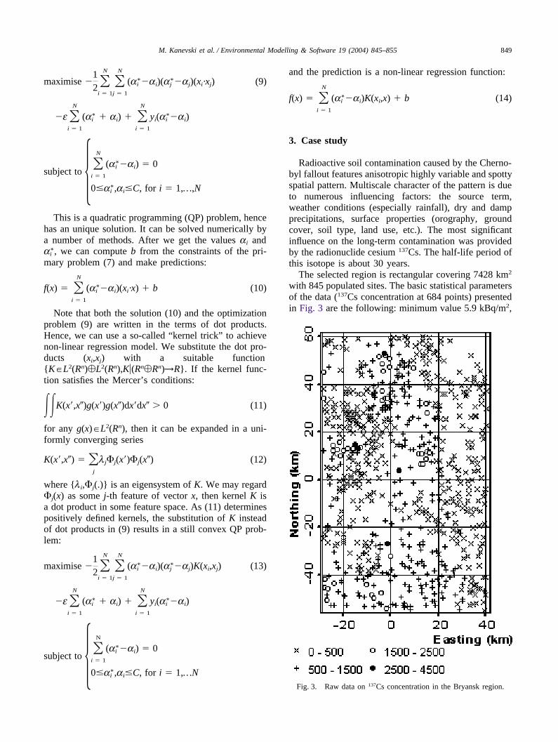
The selected region is rectangular covering 7428 km2

with 845 populated sites. The basic statistical parametersof the data (137Cs concentration at 684 points) presentedin Fig. 3 are the following: minimum value 5.9 kBq/m2,

Fig. 3. Raw data on 137Cs concentration in the Bryansk region.


mean value 571.8 kBq/m2, maximum value 4334kBq/m2, variance 315,372 kBq2/m4, skewness 2.7 andkurtosis 16.9. As usually, environmental data are posi-tively skewed and their distributions are far from normal.

The samples reflecting spatial contamination patternare the subject of exploratory spatial data analysis toaddress spatial continuity. Spatial continuity is a featureof spatial processes, which have some underlying originin the physics of the process. The presence of spatialcontinuity means that closer samples are more likelysimilar than farther ones (Issaks and Shrivastava, 1989).

Because the samples represent only one realization ofthe spatial process, some kind of stationarity assumptionis required to use statistical methods. Strong stationaritymeans that for any finite number n of sample points xi

(i = 1,…,n) and any lag h, the joint finite-dimensionaldistribution functions of Z(x1),Z(x2),…,Z(xn) are thesame as of Z(x1 + h),Z(x2 + h),…,Z(xn + h). In practice,this proposition is very hard to be detected, and as weare usually interested only in two first moments, thesecond-order stationarity assumption is enough. It is thestationarity only of the two first moments: the mean isconstant (E[Z(x)] = m = const) and covariance(Cov(x1,x2) = E[Z(x1),Z(x2)]�m2 = C(h)) exists and doesnot depend on x, but only on h.

Rather often, the real data do not follow even second-order stationarity model. Intrinsic hypothesis, which isweaker than second-order stationarity, is enough to applygeostatistical tools. The intrinsic hypothesis is a processwith second-order stationarity applied for theincrements. It means that the mean of increments (alsonamed the drift):

D(h) � E[Z(x)�Z(x � h)] (15)

is constant and D(h) = 0 and does not depend on x andh, and the variance of increments (2g(h) = var[Z(x +h)�Z(x)]) exists and does not depend on x, only on h.

The drift D(h) can be an indicator of data obedienceto the intrinsic hypothesis. Such a deduction can bemade, for example, when the value of the drift D(h)fluctuates around zero (the drift is supposed to be zerowhatsoever the position of h in the domain). If D(h)increases/decreases with the augmentation of the lengthof the separation vector h (see Fig. 4), then the data donot follow the intrinsic hypotheses. It can mean that thedata have systematic trend. In such cases, the variogrammodeling and the following common geostatistical pre-diction will result in misleading results. To handle thisproblem, the trend must be removed from the data in thefirst place. Here, the machine learning algorithms havebeen used to model the trend in the data.

Cell declustering was used for splitting data into train-ing and testing sets to provide efficient ML learning. Theregion was divided into rectangular cells by a regulargrid and one or several points were selected at randomfrom each cell. The testing dataset was obtained in this

Fig. 4. The drift of 137Cs data.

way, and the rest of the data formed the training set.Thus, testing set represents regional data. Of course, thetraining set in this case is somewhat clustered that isnot so good for the MLA training. However, using thebackward selection (i.e. picking out the points for train-ing dataset by the declustering and to consider the restas testing one) is impossible to obtain a representativetesting set. The procedure of selection was carried outseveral times with different cell sizes and with varyingnumbers of the selected points from each cell. Since itis difficult to control both testing and training datasets,more attention was paid to the similarity of the trainingdata set to the initial data structures of all data. The simi-larity was controlled by comparing summary statistics,histograms and spatial correlation structures. Similarityof spatial structures for the obtained datasets to the initialdata is even more important than statistical factors. Com-parison of the spatial structure was carried out with thehelp of variogram roses, which show anisotropy. Suchcomparison provides grounds that split (see Fig. 5) with484 training and 200 testing points is quite suitable forthe following ML modeling and it is the best of allobtained.

In the present study, MLP models with the followingparameters were used: two input neurons, describingspatial co-ordinates (X, Y), one hidden layer and outputneuron describing 137Cs contamination. Backpropagationtraining with Levenberg-Marquardt followed by conju-gate gradient algorithm was used in order to avoid localminima (Masters, 1995).

The variogram analysis of the obtained residuals forthe trained neural networks with varying number of neu-rons in the hidden layer showed that the optimal results(in the sense of modeling non-linear trends) wasobtained by using MLP with five neurons in a singlehidden layer. Further increase of the number of hiddenneurons leads to extracting more detailed local peculiari-ties of the pattern, reflected by multiple correlation range


Fig. 5. Location of the training and testing points.

of the variogram of trend estimates. Then, MLP is usedfor 137Cs spatial prediction mapping. Predictions wereperformed on a rectangular regular grid with cell size1 × 1 km. The result for the 137Cs MLP large-scale map-ping is presented in Fig. 6.

Let us present the results of the large-scale modelingusing support vector regression approach. Several user-defined (hyper) parameters influence on the SVR model:kernel function, C, e. Gaussian radial basis functions(RBF) were found to be well suited for spatial environ-mental modeling:

K(x,x�) � exp��|x�x�|2

2s2 � (16)

Kernel parameter—bandwidth s is related to somecharacteristic correlation scales of trend model. Kernelbandwidth of 20 km is used for the presented model.Other parameters were defined as: C = 20, e = 200. This

Fig. 6. 137Cs, artificial neural network (one hidden layer with fiveneurons) spatial predictions.

choice is based both on the analysis of training and test-ing errors and the analysis of the variogram of theresulting trend model. Detailed description of the influ-ence of the parameters on the solution and tuning pro-cedure can be found in Kanevski et al. (2001). The map-ping results (trend model) are presented in Fig. 7.

Trained multilayer perceptron and support vectorregression were able to extract some information fromdata described by large-scale spatial correlations. Therest of the information—small scale spatially structuredresiduals—was analyzed and modeled using geostatist-ical conditional stochastic simulations. The obtainedresiduals are correlated with the original data and are notcorrelated with the MLA estimates (see Figs. 8 and 9).Correlation coefficients between the residuals and 137Cssample values are equal to 0.77 (for MLP residuals) and0.79 (for SVR residuals).

Exploratory variography of spatial correlation struc-tures of the Nscore transformed residuals are presentedin Figs. 10 and 11. Variograms of the Nscore transfor-med residuals can be easily modeled (fitting to theoreti-cal model) and SGSs can be applied (variogram reachesa sill and levels off). Final ML residual sequential Gaus-sian simulation results are presented as equiprobablerealizations in Figs. 12 and 13. They keep the large-scaletrend structure (from Figs. 6 and 7) and also feature dis-


Fig. 7. 137Cs, support vector regression trend modeling.

Fig. 8. Scatterplot of the MLP and SVR residuals vs. 137Cs samplevalues.

tinctive spatial variability and small-scale effects ignoredby ML models.

The similarity and dissimilarity between the realiza-tions describe spatial variability and uncertainty. Thenext step deals with the probabilistic mapping: prob-ability mapping of to be above/below some predefineddecision level. This topic relates to decision-orientedmapping of contaminated territories. Usually, hundreds

Fig. 9. Scatterplot of the MLP and SVR residuals vs. MLP and SVRestimates, respectively.

Fig. 10. Nscore omni-directional variogram and the variogram modelof the MLP residuals.

Fig. 11. Nscore omni-directional variogram and the variogram modelof the SVR residuals.


Fig. 12. Mapping of 137Cs with neural network residual sequentialGaussian simulations model (NNRSGS).

of simulated models (realizations) are generated. Post-processing of realizations gives rich variety of outputs,one of them is the probability/risk map. Probability mapsof exceeding level 800 kBq/m2 obtained with neuralnetwork/support vector regression residual sequentialGaussian simulation models are presented in Figs. 14and 15, respectively. This is an important advancedinformation for the real decision-making process.

4. Discussion

The final stage deals with the validation of the MLresidual sequential Gaussian simulation results. compari-sons with geostatistical prediction models were carriedout. The proposed models give comparable or betterresults on different data sets. A comparison between pro-posed models (NNRSGS and SVRRSGS) was also car-ried out at the testing points. As a result, the NNRSGSmodel gives better results than the SVRRSGS model interms of testing error and summary statistics of testingdistribution. Comprehensive comparison with other MLmethods is a topic of further research.

Several important points should be mentioned:

(1) Analysis of the residuals is important also in case

Fig. 13. Mapping of 137Cs with support vector regression residualsequential Gaussian simulations model (SVRRSGS).

when only ML mapping is applied. This helps tounderstand the quality of the results. If there is nospatial correlation in the residuals, it means that allspatial information from data have been extractedand ML can be used for prediction mapping as well.

(2) Robustness of the approach: how it is sensitive tothe selection of the ML architecture and learningalgorithm. Chernov et al. (1999) demonstrated therobustness of MLP with varying number of neuronson validation data. Also, it was shown that MLP ismore sensitive towards selection of the training setthan towards the number of neurons. The samerobust behavior in the case presented in this studyhas been obtained both for MLP and SVR (varyingmodel parameters). So, we can choose the simplestML models capable to learn and catch non-lineartrends.

Usually, accuracy test (analysis of the residuals) hasbeen used for the analysis and description of what waslearned by ML. Accuracy test measures correlationbetween the training data and the MLA predictions atthe same points.

(3) Data clustering is a well-known problem in spatialdata analysis (Deutsch and Journel, 1998). This


Fig. 14. Probability of exceeding level of 800 kBq/m2 forNNRSGS model.

problem is related to the spatial representativity ofdata. The influence of clustering on the efficiency ofML algorithms should be studied in detail.

5. Conclusions

New non-stationary NNRSGS and SVRRSGS modelsfor the analysis and mapping of spatially distributed datawere developed. Non-linear trends in environmental datacan be efficiently modeled by a three layer perceptron.Combinations of ML and geostatistical models gave riseto the decision-oriented risk and probabilistic mapping.Promising results presented are based on the unique casestudy: soil contamination by the most radiologicallyimportant Chernobyl radionuclide. Other kinds of ANNmodels (in particular local approximators) can be usedwith possible modifications in the proposed framework.ML based models are preferable to pure geostatisticalmethods because the latter have limitations due to pres-ence of non-linear trends in data, which are difficult tomodel. Computational costs of the method are rathercheap for a typical geostatistical problem. But the appli-cation of the method needs deep expert knowledge ingeostatistical modeling. Further, extensions of the

Fig. 15. Probability of exceeding level of 800 kBq/m2 forSVRRSGS model.

approach may deal with multivariate cases as long asML algorithms are capable of dealing with multivariateinformation and can integrate different types of data.Extension of the model to image processing requiresimproving and adaptation of the algorithms, especiallyfrom ML side. Recent developments in ML algorithmsimplementations, see e.g. http://www.torch.ch, are prom-ising from the computational point of view.

The analysis and presentation of the results as well asMLP and Gaussian simulation modeling were performedwith the help of GEOSTAT OFFICE software (Kanevskiet al., 1999). Support vector regression modeling wascarried out with the help of GeoSVM(http://www.ibrae.ac.ru/~mkanev).

Acknowledgements

The work was supported in part by the INTAS grants99-00099, 97-31726, INTAS Aral Sea project #72,CRDF grant RG2-2236, and Russian Academy ofSciences grant for young scientists research N84, 1999.

http://www.torch.ch

http://www.ibrae.ac.ru/~mkanev


References

Bishop, C.M., 1995. Neural Networks for Pattern Recognition. Claren-don Press, Oxford.

Chernov, S., Demyanov, V., Grachev, N., Kanevski, M., Kravetski,A., Savelieva, E., Timonin, V., Maignan, M., 1999. Multiscale Pol-lution Mapping with Artificial Neural Networks and Geostastistics.Proceedings of the 5th Annual Conference of the InternationalAssociation for Mathematical Geology (IAMG’ 99). Ed. Lippartd,S.J., Nass, A., Sinding-Larsen, R., August 1999, 325-330.

Cressie, N., 1991. Statistics for Spatial Data. John Wiley & Sons,New York.

De Cort, M., Tsaturov, Yu.S., 1996. Atlas on caesium contaminationof Europe after the Chernobyl nuclear plant accident. EuropeanCommission, Report EUR 16542 EN.

Demyanov, V., Kanevski, M., Savelieva, E., Timonin, V., Chernov,S., Polishuk, V., 2000. Neural Network Residual Stochastic Cosi-mulation for Environmental Data Analysis. Proceedings of theSecond ICSC Symposium on Neural Computation (NC’2000), May2000, Berlin, Germany, 647-653.

Deutsch, C.V., Journel, A.G., 1998. GSLIB Geostatistical SoftwareLibrary and User’s Guide. Oxford University Press, New York,Oxford.

Dowd, P.A., 1994. In: Dimitrakopoulos, R. (Ed.), The Use of NeuralNetworks for Spatial Simulation, Geostatistics for the Next Cen-tury. Kluwer Academic Publishers, pp. 173–184.

Fedra, K., Winkelbauer, L., 1999. A hybrid expert system, GIS andsimulation modeling for environmental and technological risk man-agement. Environmental Decision Support Systems and ArtificialIntelligence, Technical Report WS-99-07. AAAI Press, MenloPark, CA, pp. 1–7.

Gambolati, G., Galeati, G., 1987. Comment on “analysis of nonintrin-sic spatial variability by residual kriging with application toregional groundwater levels” by Neuman and Jacobson. Mathemat-ical Geology 19, 249–257.

Gilardi, N., Bengio, S., 2000. Local machine learning models for spa-tial data analysis. IDIAP-RR 00-34.

Haas, T.C., 1996. Multivariate spatial prediction in the presence ofnonlinear trend and covariance nonstationarity. Environmetrics 7.

Haykin, S., 1999. Neural Networks. A Comprehensive Foundation,second ed. Prentice Hall International, Inc.

Isaaks, Ed.H., Shrivastava, R.M., 1989. An Introduction to AppliedGeostatistics. Oxford University Press, Oxford.

Kanevski, M., Demyanov, V., Chernov, S., Savelieva, E., Serov, A.,Timonin, V., 1999. Geostat Office for Environmental and PollutionSpatial Data Analysis. Mathematische Geologie. CPress PublishingHouse, band 3, April, pp. 73–83.

Kanevski, M., Pozdnukhov, A., Canu, S., Maignan, M., Wong, P., Shi-bli, S., 2001. Support vector machines for classification and map-ping of reservoir data. In: Soft Computing for Reservoir Charac-terization and Modeling. Springer-Verlag, pp. 531–558.

Kanevsky, M., Arutyunyan, R., Bolshov, L., Demyanov, V., Linge,I., Savelieva, E., Shershakov, V., Haas, T., Maignan, M., 1996a.Geostatistical Portrayal of the Chernobyl fallout. In: Baafi, E.Y.,Schofield, N.A. (Eds.), Geostatistics ’96, Wollongong, vol. 2.Kluwer Academic Publishers, pp. 1043–1054.

Kanevsky, M., Arutyunyan, R., Bolshov, L., Demyanov, V., Maignan,M., 1996b. Artificial neural networks and spatial estimations ofChernobyl fallout. Geoinformatics 7, 5–11.

Masters, Timothy, 1995. Advanced Algorithms for Neural Networks.A C++ Sourcebook. John Wiley & Sons, Inc.

Neuman, S.P., Jacobson, E.A., 1984. Analysis of nonintrinsic spatialvariability by residual kriging with application to regionalgroundwater levels. Mathematical Geology 16, 499–521.

Pelissier, R., Goreaud, F., 2001. A practical approach to the study ofspatial structure in simple cases of heterogeneous vegetation. Jour-nal of Vegetation Science 12, 99–108.

Scholkopf, B., Smola, A., 1998. Learning with Kernels. MIT Press,Cambridge, MA.

Vapnik, V., 1998. Statistical Learning Theory. John Wiley & Sons,New York.

environmental data mining and modeling based on machine learning algorithms and geostatistics

Documents