event mining: algorithms and applicationstaoli/event-mining/kdd-2017-tutorial... · event mining:...
TRANSCRIPT
Event Mining: Algorithms and Applications
Tao Li, FIU/NJUPT Larisa Shwartz, IBM Research
Genady Ya. Grabanrnik, St. John’s University
Introduction and Overview
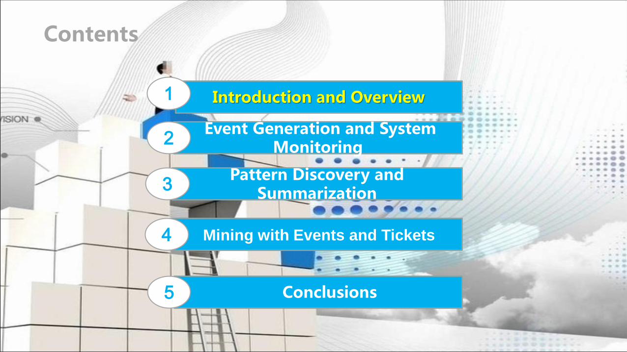
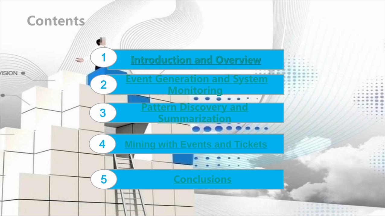
Contents
1
Event Generation and System Monitoring
2
Pattern Discovery and Summarization
3
Conclusions 5
Mining with Events and Tickets 4
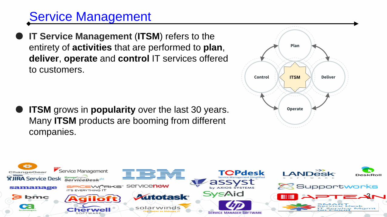
● IT Service Management (ITSM) refers to the
entirety of activities that are performed to plan,
deliver, operate and control IT services offered
to customers.
● ITSM grows in popularity over the last 30 years.
Many ITSM products are booming from different
companies.
3
Service Management
ITSM Deliver Control
Operate
Plan
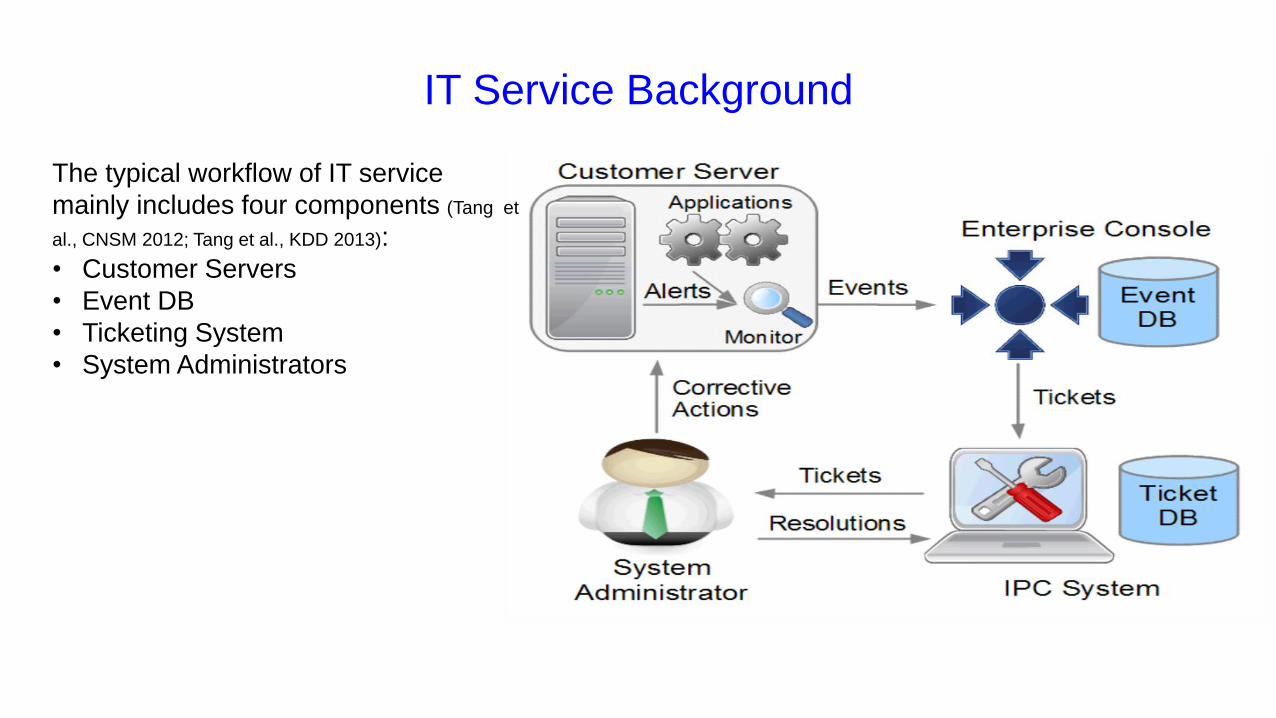
IT Service Background
The typical workflow of IT service
mainly includes four components (Tang et
al., CNSM 2012; Tang et al., KDD 2013):
• Customer Servers
• Event DB
• Ticketing System
• System Administrators
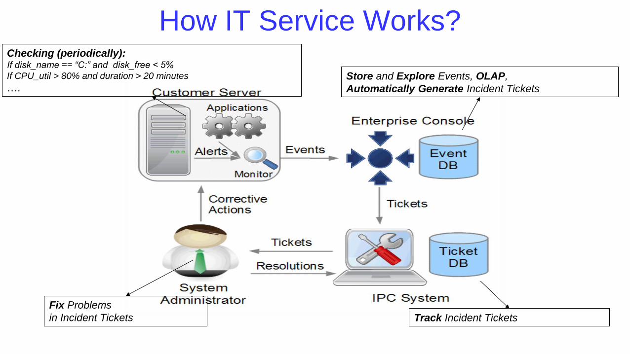
How IT Service Works? Checking (periodically): If disk_name == “C:” and disk_free < 5%
If CPU_util > 80% and duration > 20 minutes
…. Store and Explore Events, OLAP,
Automatically Generate Incident Tickets
Track Incident Tickets
Fix Problems
in Incident Tickets
A typical workflow of IT Service Management involves an appropriate
mix of people, process, information and technology.
6
The Workflow:Data Perspective
1.Hundreds of time series
2.Hundreds of event types
3.Hundreds of categories
4.Millions of instances over time
labor-intensive
Problem
Determination Problem
Diagnosis
Problem
Resolution
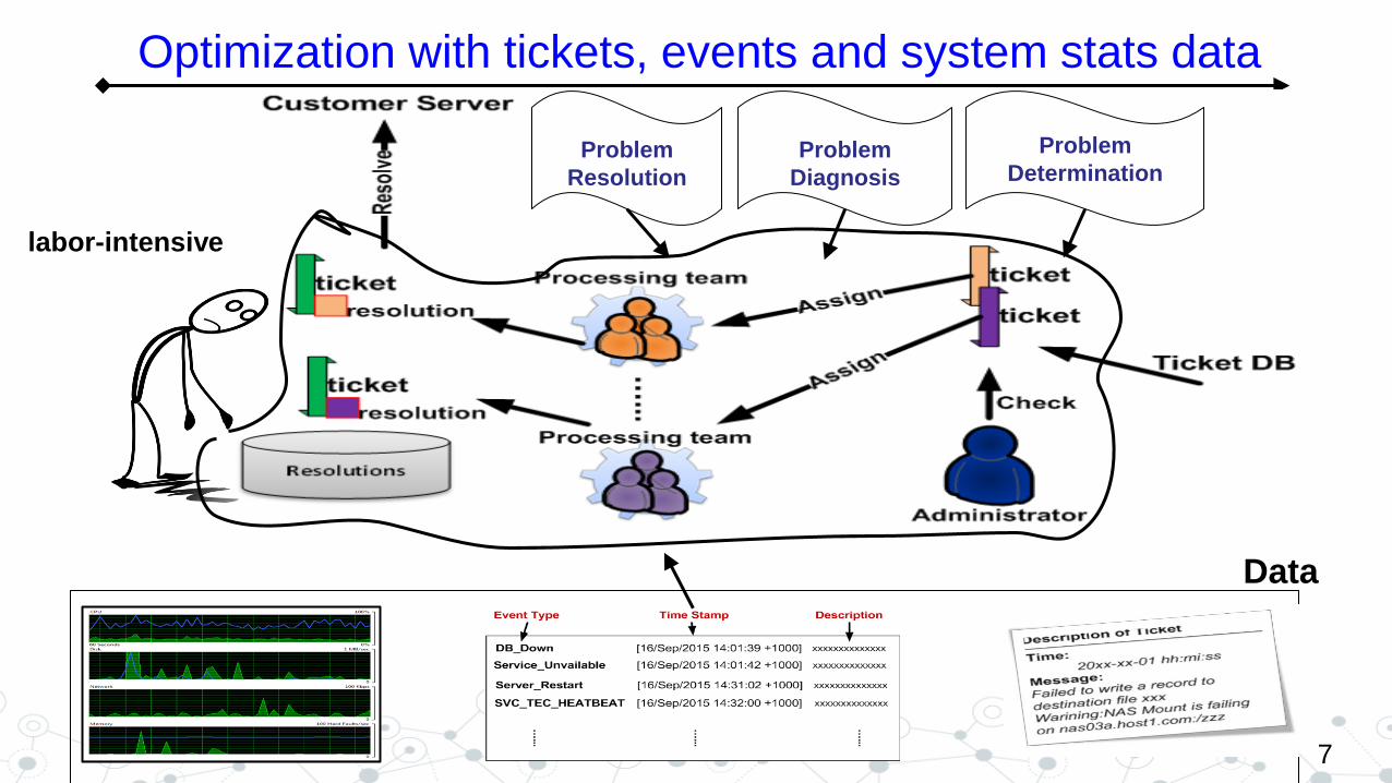
7
Optimization with tickets, events and system stats data
Problem
Determination Problem
Diagnosis
Problem
Resolution
Data
labor-intensive
Maximal automation
of
routine IT maintenance procedures is one of ultimate goals of IT
service management optimization
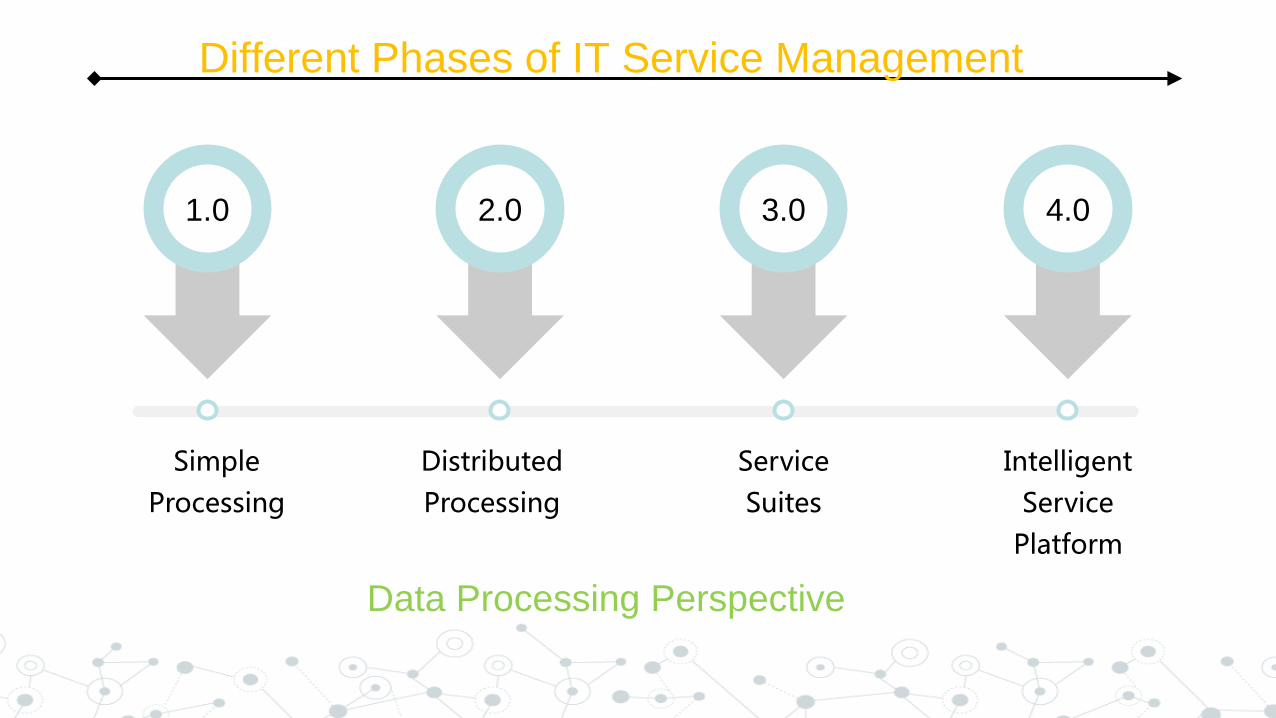
1.0
Simple
Processing
2.0
Distributed
Processing
3.0
Service
Suites
4.0
Intelligent
Service
Platform
Different Phases of IT Service Management
Data Processing Perspective

data size is relatively small: MB/GB
Using testing tools(ping,traceroute,SNMP,tcpdump)or monitoring
tools (e.g., Zabbix)
problem identification、problem localization、 problem resolution,
Phase 1.0
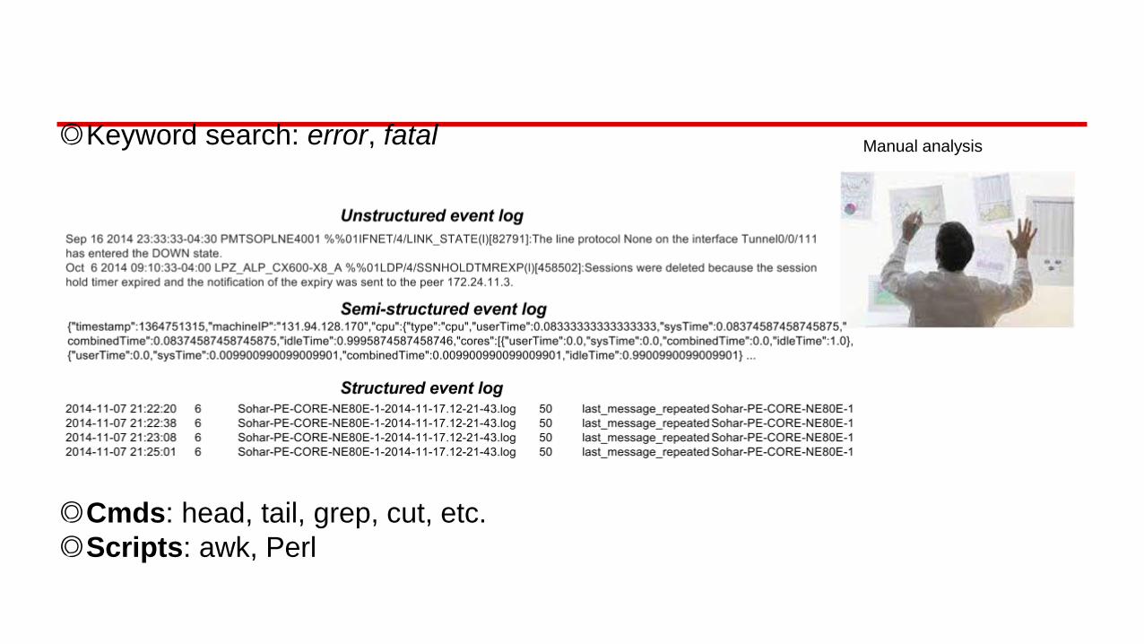
◎Keyword search: error, fatal
◎Cmds: head, tail, grep, cut, etc.
◎Scripts: awk, Perl
Manual analysis
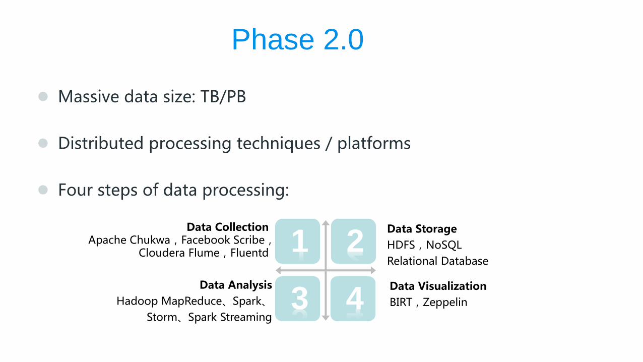
Massive data size: TB/PB
Distributed processing techniques / platforms
Four steps of data processing:
Phase 2.0
Data Storage
HDFS,NoSQL
Relational Database
Data Visualization
BIRT,Zeppelin
Data Collection Apache Chukwa,Facebook Scribe,
Cloudera Flume,Fluentd
Data Analysis
Hadoop MapReduce、Spark、
Storm、Spark Streaming
1
4 3
2
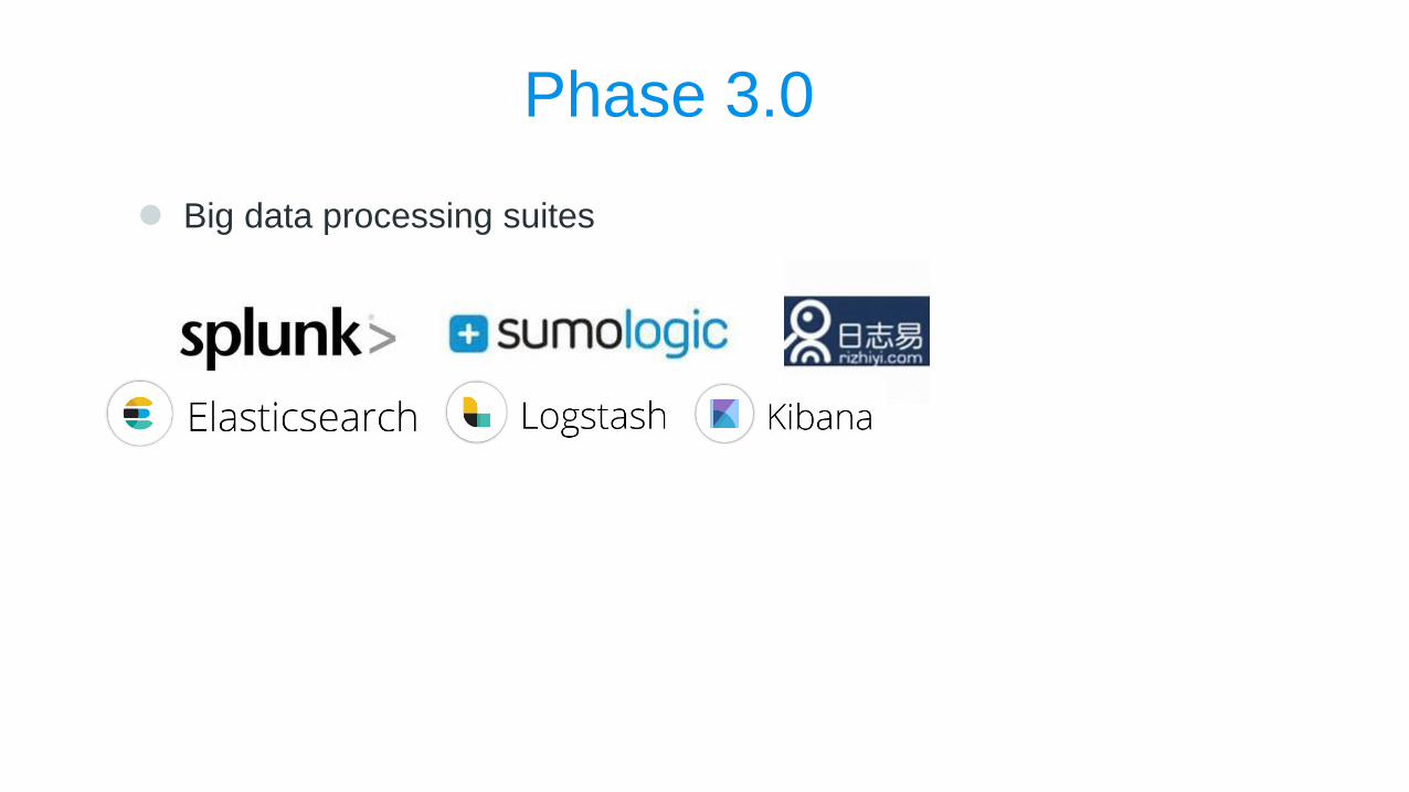
Phase 3.0
Big data processing suites

Phase 4.0
Add more intelligent techniques (AI, Machine Learning and Data Mining Techniques) on top of the existing suites
Natural Language
Processing
Big Data
Mining
Machine
Learning
Efficient Analysis
Algorithms
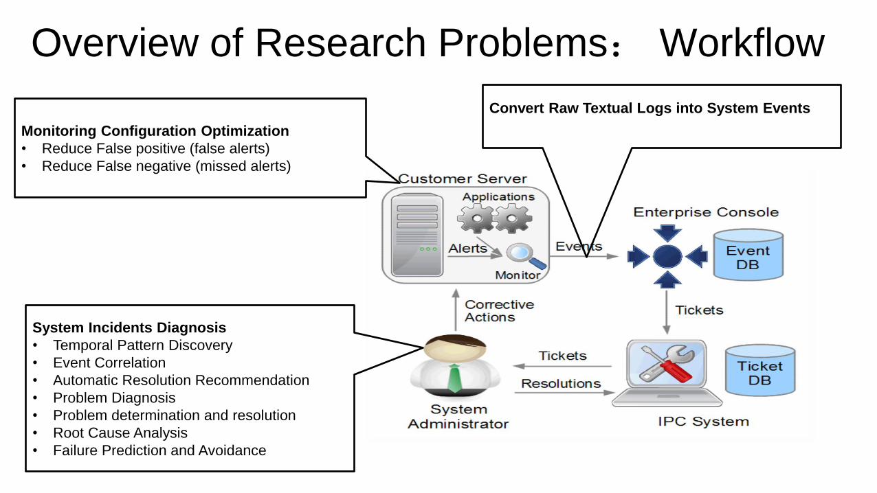
Overview of Research Problems: Workflow
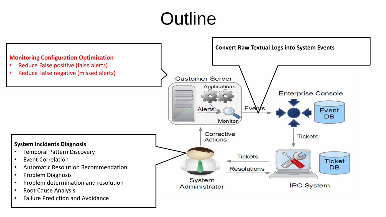
Monitoring Configuration Optimization
• Reduce False positive (false alerts)
• Reduce False negative (missed alerts)
System Incidents Diagnosis
• Temporal Pattern Discovery
• Event Correlation
• Automatic Resolution Recommendation
• Problem Diagnosis
• Problem determination and resolution
• Root Cause Analysis
• Failure Prediction and Avoidance
Convert Raw Textual Logs into System Events
16
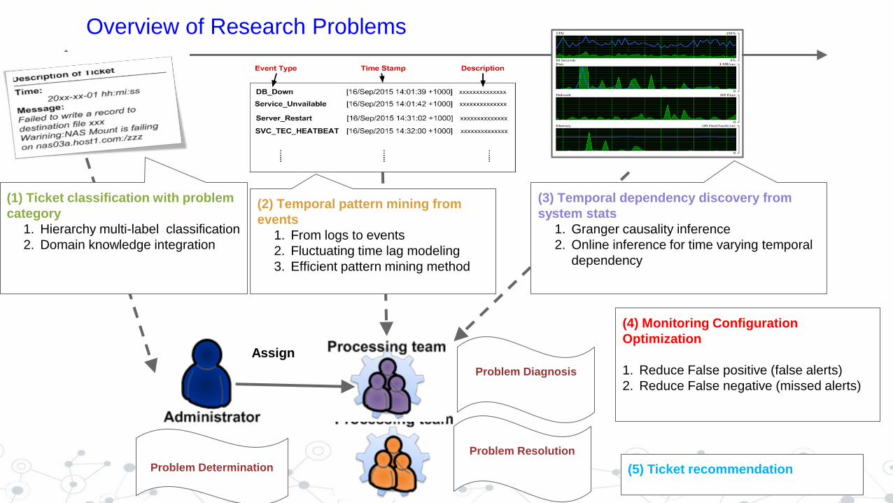
Overview of Research Problems
Problem Determination
Problem Resolution
Problem Diagnosis
Assign
(1) Ticket classification with problem
category
1. Hierarchy multi-label classification
2. Domain knowledge integration
(2) Temporal pattern mining from
events
1. From logs to events
2. Fluctuating time lag modeling
3. Efficient pattern mining method
(3) Temporal dependency discovery from
system stats
1. Granger causality inference
2. Online inference for time varying temporal
dependency
(4) Monitoring Configuration
Optimization
1. Reduce False positive (false alerts)
2. Reduce False negative (missed alerts)
(5) Ticket recommendation
Introduction and Overview
Contents
1
Event Generation and System Monitoring
2
Pattern Discovery and Summarization
3
Conclusions 5
Mining with Events and Tickets 4
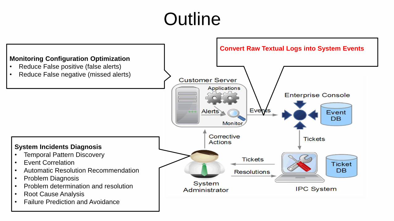
Outline
Monitoring Configuration Optimization
• Reduce False positive (false alerts)
• Reduce False negative (missed alerts)
System Incidents Diagnosis
• Temporal Pattern Discovery
• Event Correlation
• Automatic Resolution Recommendation
• Problem Diagnosis
• Problem determination and resolution
• Root Cause Analysis
• Failure Prediction and Avoidance
Convert Raw Textual Logs into System Events
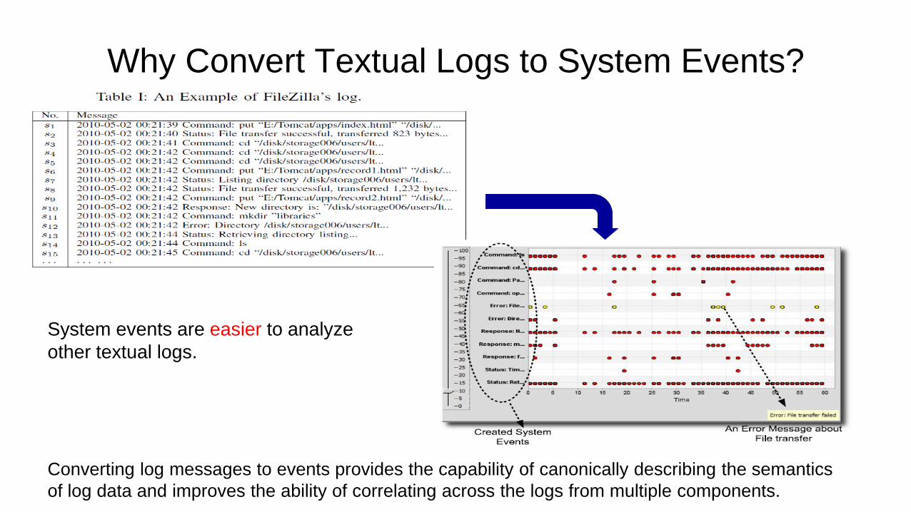
Why Convert Textual Logs to System Events?
System events are easier to analyze
other textual logs.
Converting log messages to events provides the capability of canonically describing the semantics
of log data and improves the ability of correlating across the logs from multiple components.
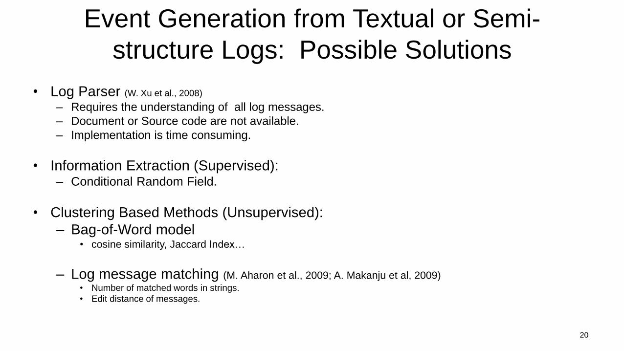
Event Generation from Textual or Semi-
structure Logs: Possible Solutions
• Log Parser (W. Xu et al., 2008) – Requires the understanding of all log messages.
– Document or Source code are not available.
– Implementation is time consuming.
• Information Extraction (Supervised): – Conditional Random Field.
• Clustering Based Methods (Unsupervised):
– Bag-of-Word model • cosine similarity, Jaccard Index…
– Log message matching (M. Aharon et al., 2009; A. Makanju et al, 2009) • Number of matched words in strings.
• Edit distance of messages.
20
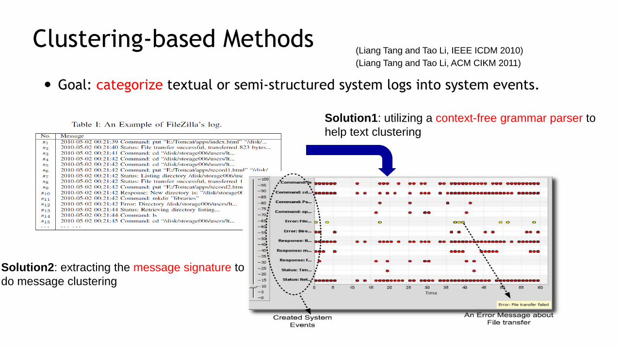
Clustering-based Methods
Goal: categorize textual or semi-structured system logs into system events.
21
Solution1: utilizing a context-free grammar parser to
help text clustering
Solution2: extracting the message signature to
do message clustering
(Liang Tang and Tao Li, IEEE ICDM 2010)
(Liang Tang and Tao Li, ACM CIKM 2011)
Tree-Structure based Clustering
Basic Idea
1) Convert the log messages into tree-structured data,
where each node is a segment of message.
2) Do clustering based on tree-structured data.
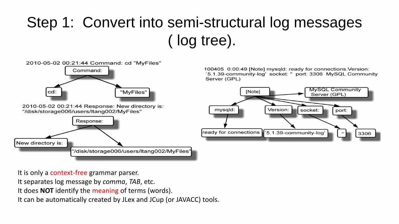
Step 1: Convert into semi-structural log messages
( log tree).
It is only a context-free grammar parser. It separates log message by comma, TAB, etc. It does NOT identify the meaning of terms (words). It can be automatically created by JLex and JCup (or JAVACC) tools.
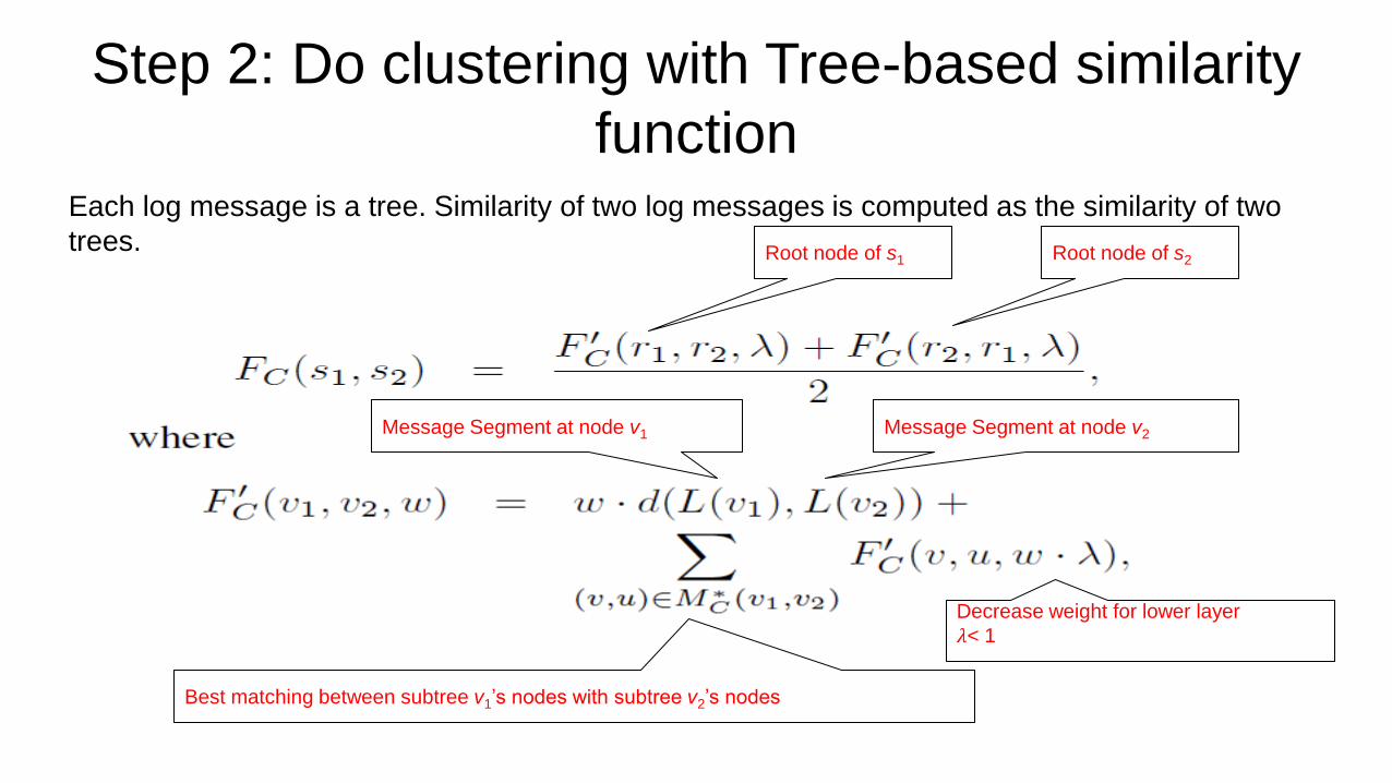
Step 2: Do clustering with Tree-based similarity
function Each log message is a tree. Similarity of two log messages is computed as the similarity of two
trees. Root node of s1 Root node of s2
Message Segment at node v1 Message Segment at node v2
Best matching between subtree v1’s nodes with subtree v2’s nodes
Decrease weight for lower layer
𝜆< 1
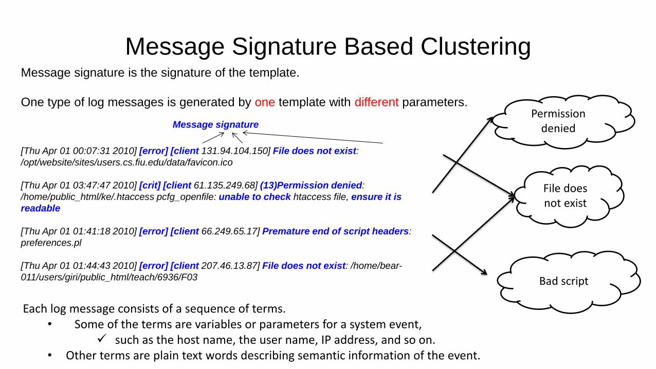
Message Signature Based Clustering
[Thu Apr 01 00:07:31 2010] [error] [client 131.94.104.150] File does not exist:
/opt/website/sites/users.cs.fiu.edu/data/favicon.ico
[Thu Apr 01 03:47:47 2010] [crit] [client 61.135.249.68] (13)Permission denied:
/home/public_html/ke/.htaccess pcfg_openfile: unable to check htaccess file, ensure it is
readable
[Thu Apr 01 01:41:18 2010] [error] [client 66.249.65.17] Premature end of script headers:
preferences.pl
[Thu Apr 01 01:44:43 2010] [error] [client 207.46.13.87] File does not exist: /home/bear-
011/users/giri/public_html/teach/6936/F03
File does not exist
Permission denied
Bad script
Message signature is the signature of the template.
One type of log messages is generated by one template with different parameters.
Message signature
Each log message consists of a sequence of terms. • Some of the terms are variables or parameters for a system event,
such as the host name, the user name, IP address, and so on. • Other terms are plain text words describing semantic information of the event.
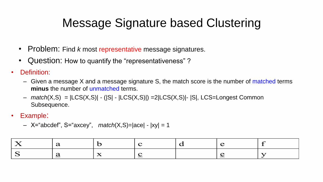
Message Signature based Clustering
• Problem: Find k most representative message signatures.
• Question: How to quantify the “representativeness” ?
• Definition:
– Given a message X and a message signature S, the match score is the number of matched terms
minus the number of unmatched terms.
– match(X,S) = |LCS(X,S)| - (|S| - |LCS(X,S)|) =2|LCS(X,S)|- |S|, LCS=Longest Common
Subsequence.
• Example: – X=“abcdef”, S=“axcey”, match(X,S)=|ace| - |xy| = 1
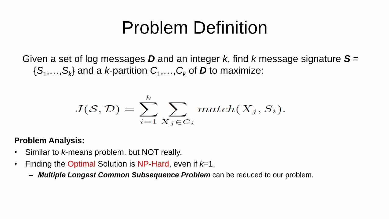
Problem Definition
Given a set of log messages D and an integer k, find k message signature S =
{S1,…,Sk} and a k-partition C1,…,Ck of D to maximize:
Problem Analysis:
• Similar to k-means problem, but NOT really.
• Finding the Optimal Solution is NP-Hard, even if k=1.
– Multiple Longest Common Subsequence Problem can be reduced to our problem.
Outline
Monitoring Configuration Optimization • Reduce False positive (false alerts) • Reduce False negative (missed alerts)
System Incidents Diagnosis • Temporal Pattern Discovery • Event Correlation • Automatic Resolution Recommendation • Problem Diagnosis • Problem determination and resolution • Root Cause Analysis • Failure Prediction and Avoidance
Convert Raw Textual Logs into System Events
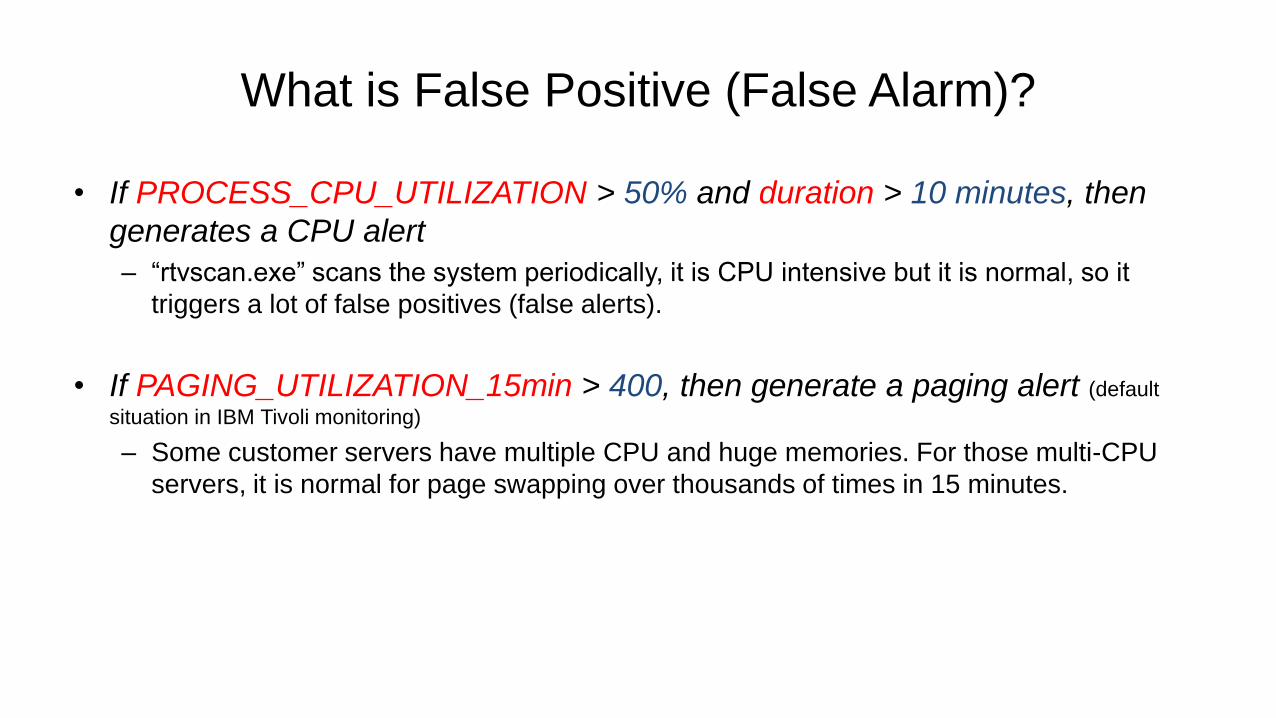
What is False Positive (False Alarm)?
• If PROCESS_CPU_UTILIZATION > 50% and duration > 10 minutes, then
generates a CPU alert
– “rtvscan.exe” scans the system periodically, it is CPU intensive but it is normal, so it
triggers a lot of false positives (false alerts).
• If PAGING_UTILIZATION_15min > 400, then generate a paging alert (default
situation in IBM Tivoli monitoring)
– Some customer servers have multiple CPU and huge memories. For those multi-CPU
servers, it is normal for page swapping over thousands of times in 15 minutes.
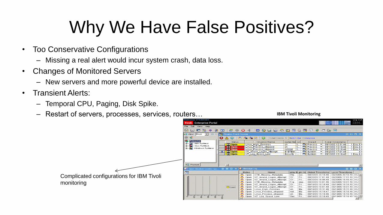
Why We Have False Positives? • Too Conservative Configurations
– Missing a real alert would incur system crash, data loss.
• Changes of Monitored Servers
– New servers and more powerful device are installed.
• Transient Alerts:
– Temporal CPU, Paging, Disk Spike.
– Restart of servers, processes, services, routers… IBM Tivoli Monitoring
Complicated configurations for IBM Tivoli
monitoring
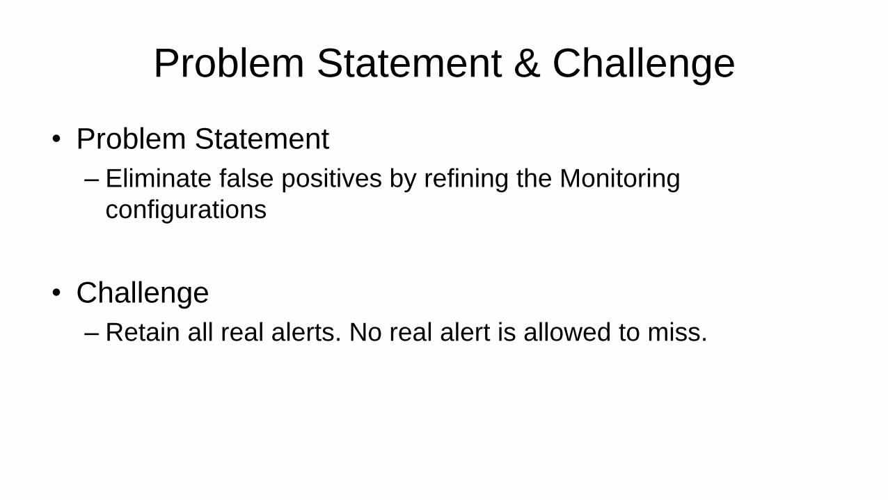
Problem Statement & Challenge
• Problem Statement
– Eliminate false positives by refining the Monitoring
configurations
• Challenge
– Retain all real alerts. No real alert is allowed to miss.
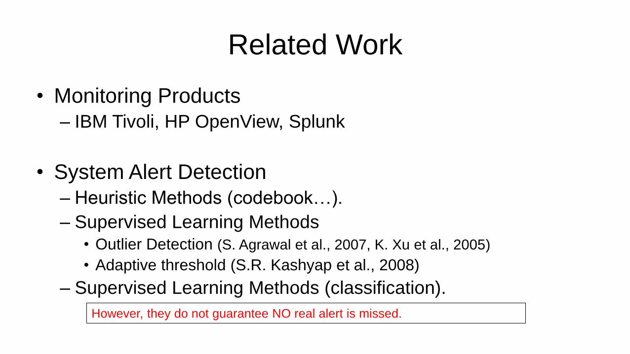
Related Work
• Monitoring Products
– IBM Tivoli, HP OpenView, Splunk
• System Alert Detection
– Heuristic Methods (codebook…).
– Supervised Learning Methods • Outlier Detection (S. Agrawal et al., 2007, K. Xu et al., 2005)
• Adaptive threshold (S.R. Kashyap et al., 2008)
– Supervised Learning Methods (classification).
However, they do not guarantee NO real alert is missed.
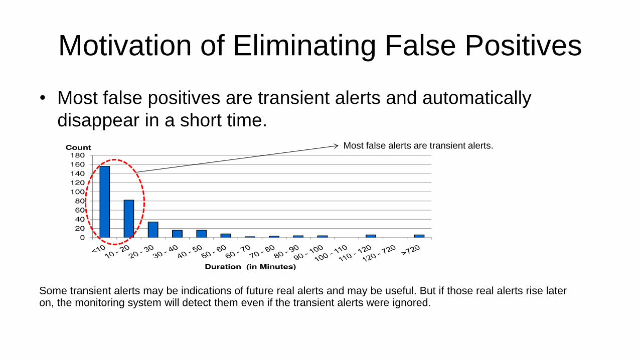
Motivation of Eliminating False Positives
• Most false positives are transient alerts and automatically
disappear in a short time.
Some transient alerts may be indications of future real alerts and may be useful. But if those real alerts rise later on, the monitoring system will detect them even if the transient alerts were ignored.
Most false alerts are transient alerts.
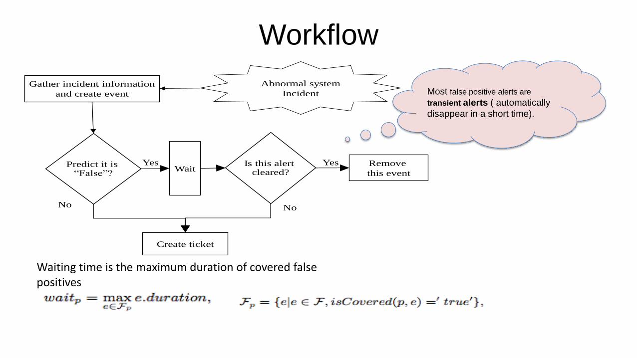
Workflow
Gather incident information
and create event
Create ticket
Predict it is “False”?
WaitIs this alert
cleared?
Yes Yes Remove
this event
NoNo
Abnormal system
Incident Most false positive alerts are
transient alerts ( automatically
disappear in a short time).
Waiting time is the maximum duration of covered false positives
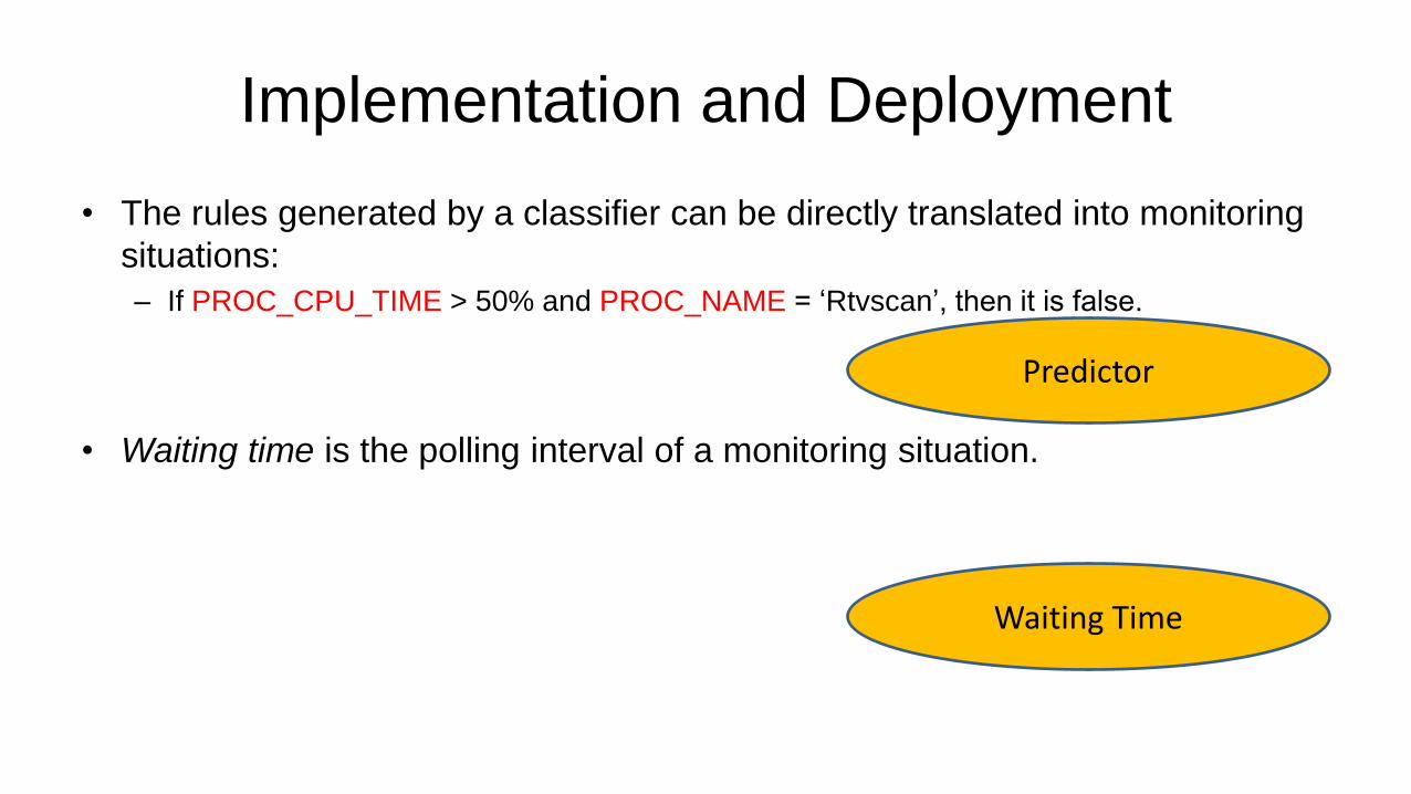
Implementation and Deployment
• The rules generated by a classifier can be directly translated into monitoring
situations:
– If PROC_CPU_TIME > 50% and PROC_NAME = ‘Rtvscan’, then it is false.
• Waiting time is the polling interval of a monitoring situation.
Predictor
Waiting Time
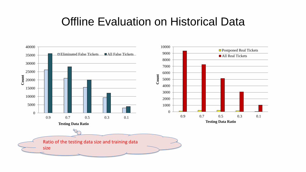
Offline Evaluation on Historical Data
0
5000
10000
15000
20000
25000
30000
35000
40000
0.9 0.7 0.5 0.3 0.1
Cou
nt
Testing Data Ratio
Eliminated False Tickets All False Tickets
0
1000
2000
3000
4000
5000
6000
7000
8000
9000
10000
0.9 0.7 0.5 0.3 0.1
Cou
nt
Testing Data Ratio
Postponed Real Tickets
All Real Tickets
Ratio of the testing data size and training data size
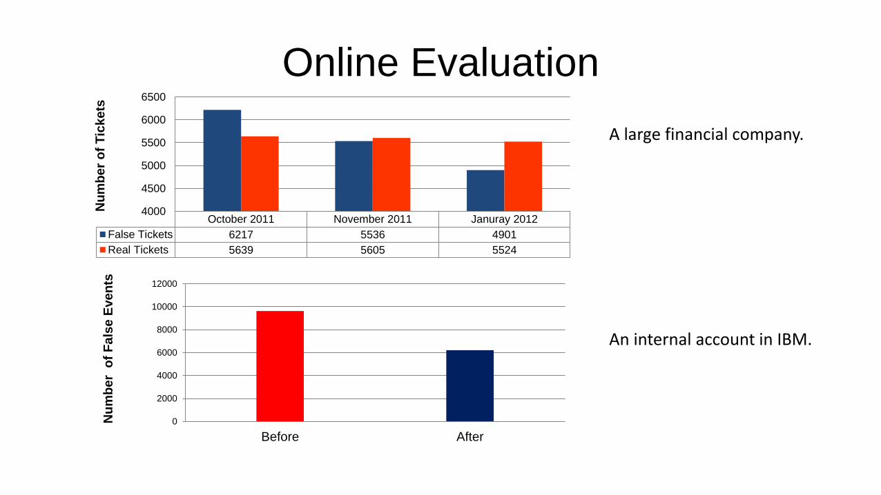
Online Evaluation
October 2011 November 2011 Januray 2012
False Tickets 6217 5536 4901
Real Tickets 5639 5605 5524
4000
4500
5000
5500
6000
6500N
um
be
r o
f T
ick
ets
0
2000
4000
6000
8000
10000
12000
Before After
Nu
mb
er
of
Fa
lse
Eve
nts
A large financial company.
An internal account in IBM.
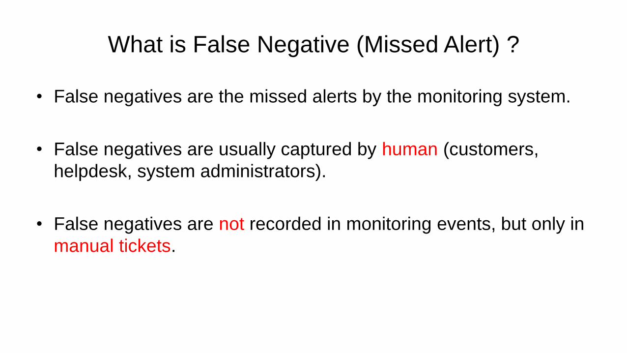
What is False Negative (Missed Alert) ?
• False negatives are the missed alerts by the monitoring system.
• False negatives are usually captured by human (customers,
helpdesk, system administrators).
• False negatives are not recorded in monitoring events, but only in
manual tickets.
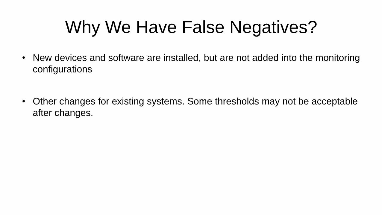
Why We Have False Negatives?
• New devices and software are installed, but are not added into the monitoring
configurations
• Other changes for existing systems. Some thresholds may not be acceptable
after changes.
About False Negative
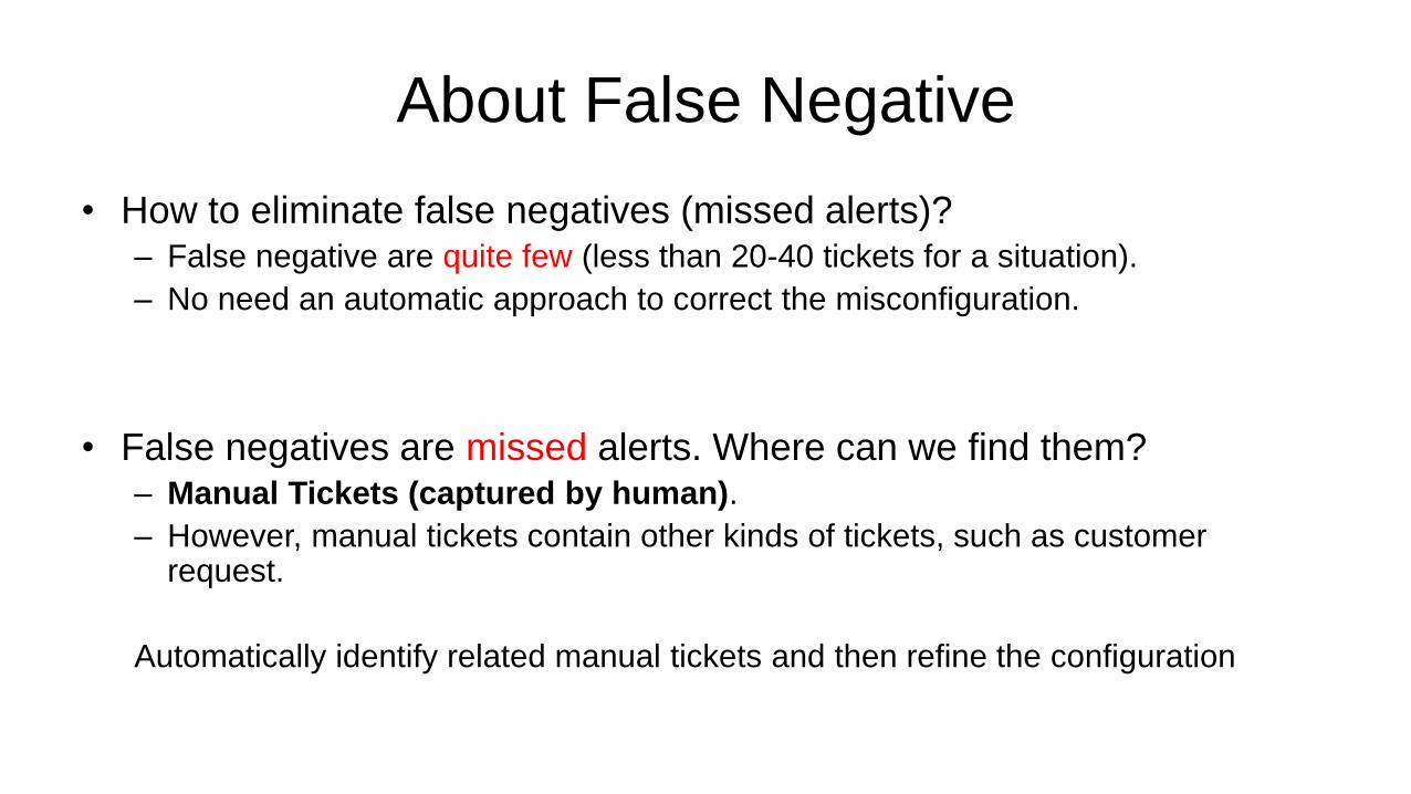
• How to eliminate false negatives (missed alerts)? – False negative are quite few (less than 20-40 tickets for a situation).
– No need an automatic approach to correct the misconfiguration.
• False negatives are missed alerts. Where can we find them? – Manual Tickets (captured by human).
– However, manual tickets contain other kinds of tickets, such as customer request.
Automatically identify related manual tickets and then refine the configuration
Problem Statement
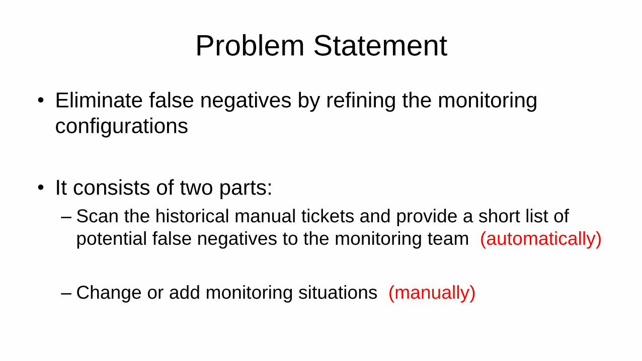
• Eliminate false negatives by refining the monitoring
configurations
• It consists of two parts:
– Scan the historical manual tickets and provide a short list of
potential false negatives to the monitoring team (automatically)
– Change or add monitoring situations (manually)

Related Work
• Reduce False Negative
– Focus on improving the accuracy of the monitoring
– No prior work is based on discovery of false negatives (Because false negatives are
missed alerts. There is no data record for tracking them).
• Text classification
– Class label “1”: a missed alert; class label “0”: other issues, such as customer request.
Features are the words in the ticket description.
– Imbalanced classification: Cost-sensitive and over-sampling.
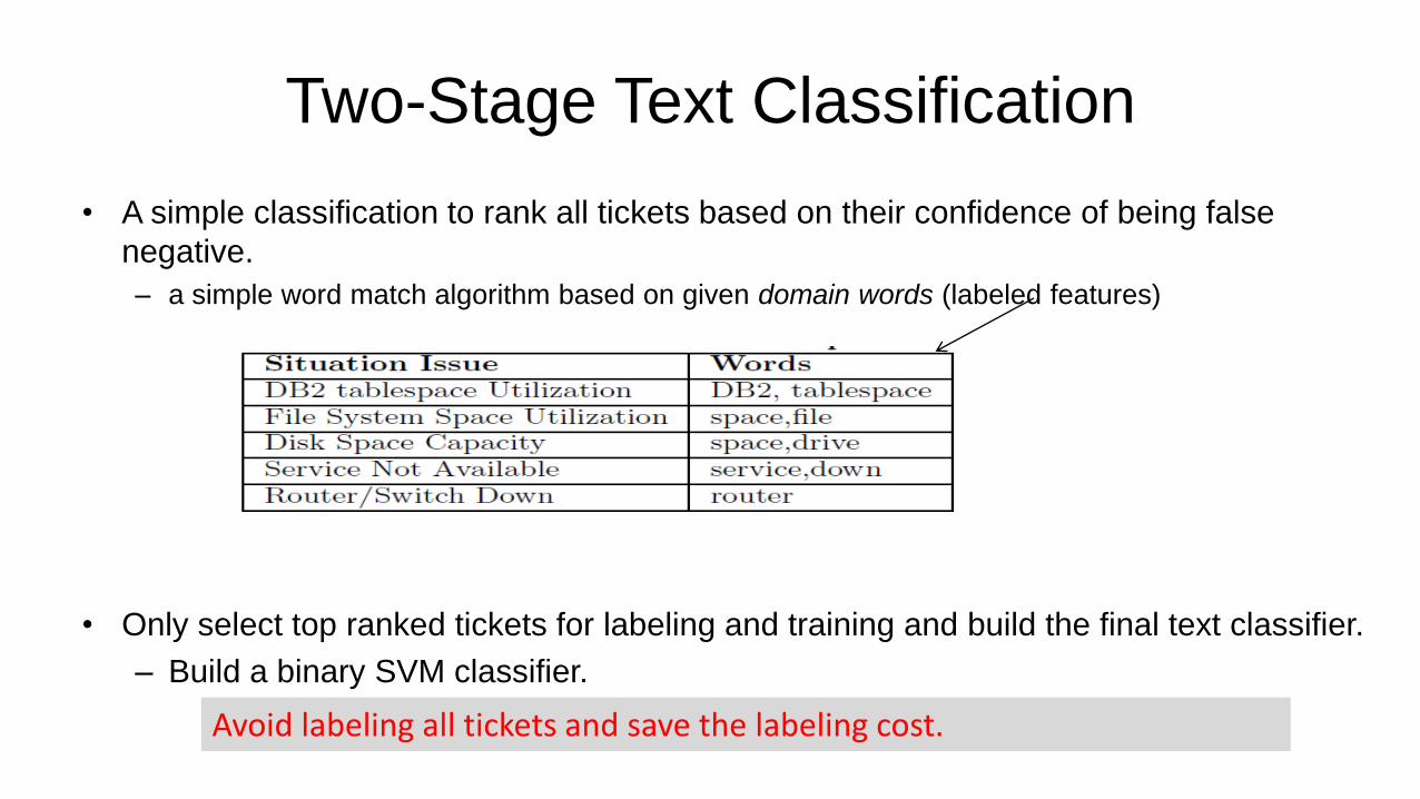
Two-Stage Text Classification
• A simple classification to rank all tickets based on their confidence of being false
negative.
– a simple word match algorithm based on given domain words (labeled features)
• Only select top ranked tickets for labeling and training and build the final text classifier.
– Build a binary SVM classifier.
Avoid labeling all tickets and save the labeling cost.
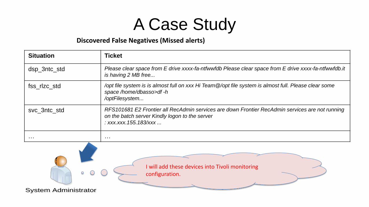
A Case Study
Situation Ticket
dsp_3ntc_std Please clear space from E drive xxxx-fa-ntfwwfdb Please clear space from E drive xxxx-fa-ntfwwfdb.it
is having 2 MB free...
fss_rlzc_std /opt file system is is almost full on xxx Hi Team@/opt file system is almost full. Please clear some
space /home/dbasso>df -h
/optFilesystem...
svc_3ntc_std RFS101681 E2 Frontier all RecAdmin services are down Frontier RecAdmin services are not running
on the batch server Kindly logon to the server
: xxx.xxx.155.183/xxx ...
… …
Discovered False Negatives (Missed alerts)
I will add these devices into Tivoli monitoring configuration.
System AdministratorSystem Administrator
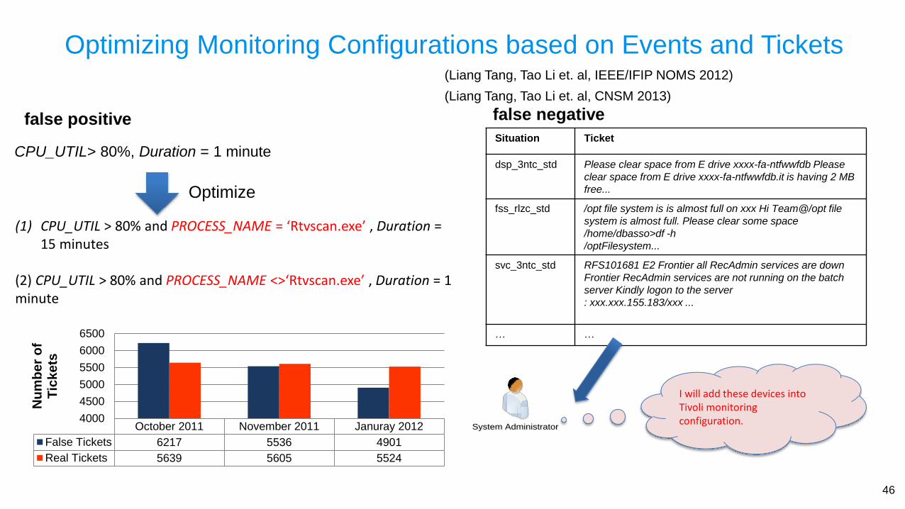
Optimizing Monitoring Configurations based on Events and Tickets
46
(Liang Tang, Tao Li et. al, IEEE/IFIP NOMS 2012)
(1) CPU_UTIL > 80% and PROCESS_NAME = ‘Rtvscan.exe’ , Duration = 15 minutes
(2) CPU_UTIL > 80% and PROCESS_NAME <>‘Rtvscan.exe’ , Duration = 1 minute
CPU_UTIL> 80%, Duration = 1 minute
Optimize
false positive
(Liang Tang, Tao Li et. al, CNSM 2013)
Situation Ticket
dsp_3ntc_std Please clear space from E drive xxxx-fa-ntfwwfdb Please
clear space from E drive xxxx-fa-ntfwwfdb.it is having 2 MB
free...
fss_rlzc_std /opt file system is is almost full on xxx Hi Team@/opt file
system is almost full. Please clear some space
/home/dbasso>df -h
/optFilesystem...
svc_3ntc_std RFS101681 E2 Frontier all RecAdmin services are down
Frontier RecAdmin services are not running on the batch
server Kindly logon to the server
: xxx.xxx.155.183/xxx ...
… …
I will add these devices into Tivoli monitoring configuration.
System AdministratorSystem AdministratorOctober 2011 November 2011 Januray 2012
False Tickets 6217 5536 4901
Real Tickets 5639 5605 5524
4000
4500
5000
5500
6000
6500
Nu
mb
er
of
Tic
ke
ts
false negative
Introduction and Overview
Contents
1
Event Generation and System Monitoring
2
Pattern Discovery and Summarization
3
Conclusions 5
Mining with Events and Tickets 4
• History on Event Mining
• Overview of Temporal Patterns
• Mining Time Lags
– Non-parametric Methods
– Parametric Methods
• Event Summarization
• Temporal Dependency
Outline
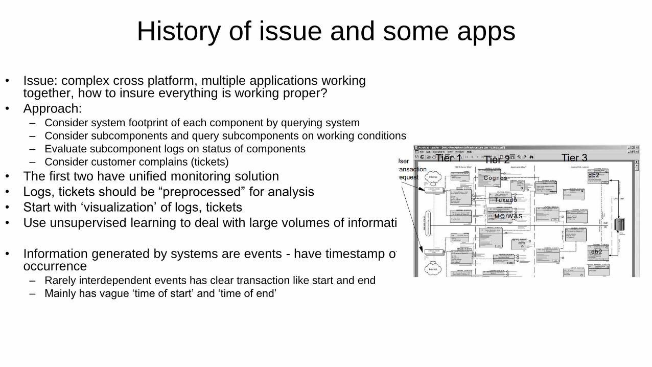
History of issue and some apps
• Issue: complex cross platform, multiple applications working together, how to insure everything is working proper?
• Approach: – Consider system footprint of each component by querying system
– Consider subcomponents and query subcomponents on working conditions
– Evaluate subcomponent logs on status of components
– Consider customer complains (tickets)
• The first two have unified monitoring solution
• Logs, tickets should be “preprocessed” for analysis
• Start with ‘visualization’ of logs, tickets
• Use unsupervised learning to deal with large volumes of information
• Information generated by systems are events - have timestamp of occurrence
– Rarely interdependent events has clear transaction like start and end
– Mainly has vague ‘time of start’ and ‘time of end’
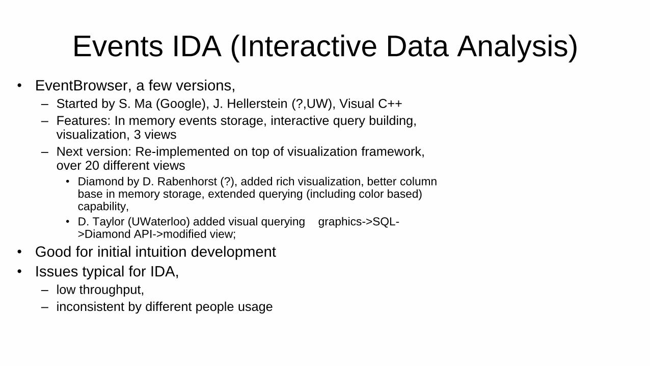
Events IDA (Interactive Data Analysis) • EventBrowser, a few versions,
– Started by S. Ma (Google), J. Hellerstein (?,UW), Visual C++
– Features: In memory events storage, interactive query building, visualization, 3 views
– Next version: Re-implemented on top of visualization framework, over 20 different views
• Diamond by D. Rabenhorst (?), added rich visualization, better column base in memory storage, extended querying (including color based) capability,
• D. Taylor (UWaterloo) added visual querying graphics->SQL->Diamond API->modified view;
• Good for initial intuition development
• Issues typical for IDA,
– low throughput,
– inconsistent by different people usage
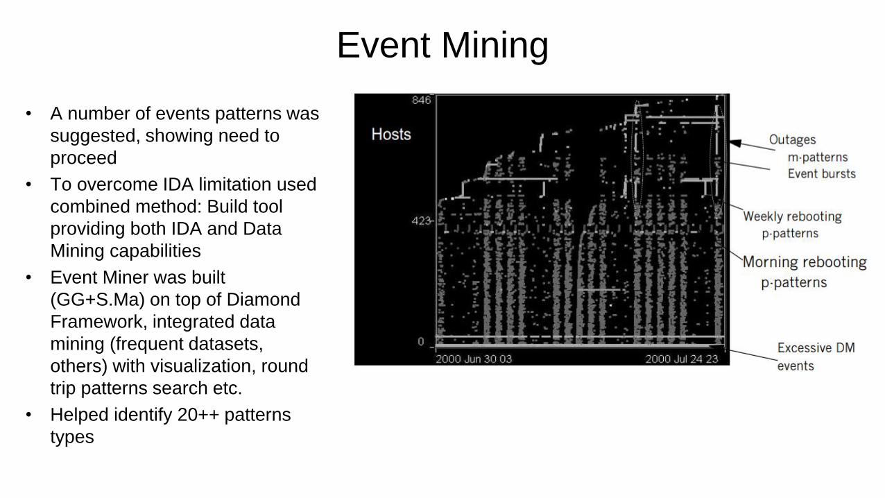
Event Mining
• A number of events patterns was
suggested, showing need to
proceed
• To overcome IDA limitation used
combined method: Build tool
providing both IDA and Data
Mining capabilities
• Event Miner was built
(GG+S.Ma) on top of Diamond
Framework, integrated data
mining (frequent datasets,
others) with visualization, round
trip patterns search etc.
• Helped identify 20++ patterns
types
52
Pattern Discovery I
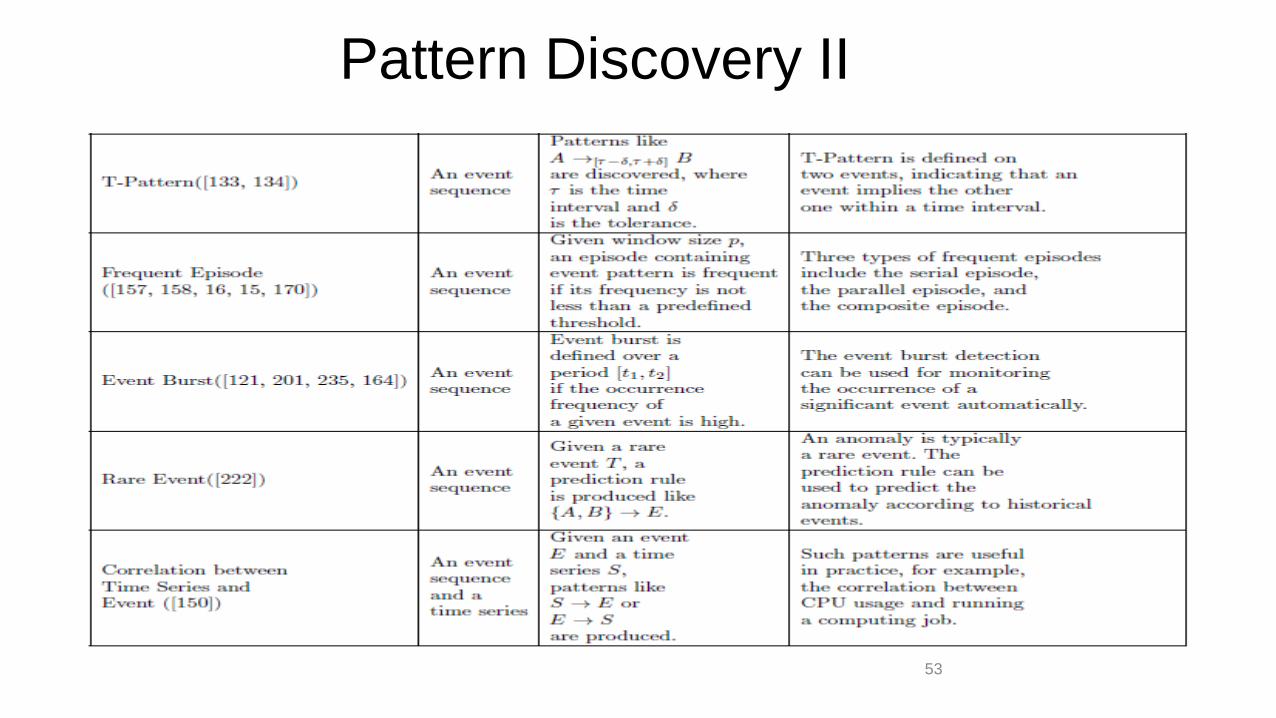
53
Pattern Discovery II
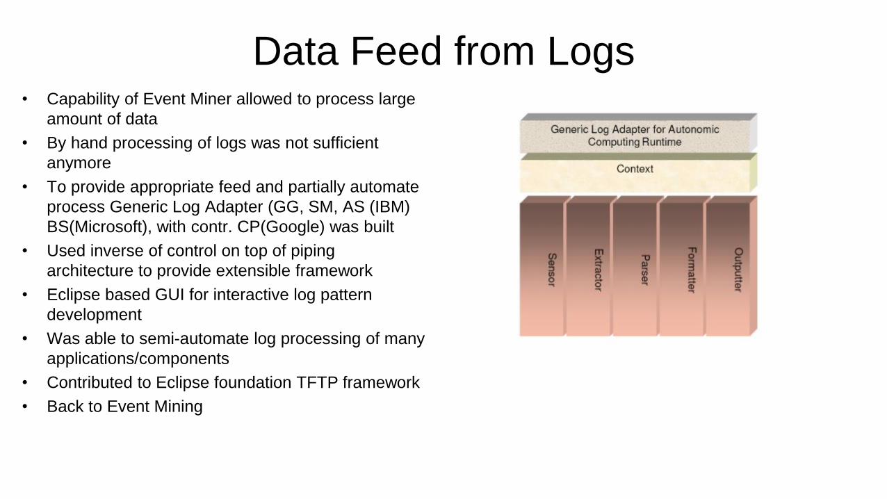
Data Feed from Logs • Capability of Event Miner allowed to process large
amount of data
• By hand processing of logs was not sufficient
anymore
• To provide appropriate feed and partially automate
process Generic Log Adapter (GG, SM, AS (IBM)
BS(Microsoft), with contr. CP(Google) was built
• Used inverse of control on top of piping
architecture to provide extensible framework
• Eclipse based GUI for interactive log pattern
development
• Was able to semi-automate log processing of many
applications/components
• Contributed to Eclipse foundation TFTP framework
• Back to Event Mining
• History on Event Mining
• Overview of Temporal Patterns
• Mining Time Lags
– Non-parametric Methods
– Parametric Methods
• Event Summarization
• Temporal Dependency
Outline
Mining Event Relationships • Temporal Patterns (of System Events)
– Wish: A sequence of symptom events providing a signature for identifying the root cause
– Less ambition: ‘repeating’ (sub)sequences of events
• Host Restart: “host is down” followed by “host is up” in about 10 seconds
• Failure Propagation: “a link is cut” “connection loss” “lost connection” “application terminated unexpectedly”
• Examples of Temporal Dependency
• Disk_Capacity ⟶ [5min,6min] Database, [5min, 6min] is the lag interval.
• Reflects hidden process, here may be database inserts/updates, expect normality here
3 5 7 8 9 13 1715Timestamp
(Minutes):
Disk_Capactiy
Database
A
B B
A A
BB
665
C C CC CApp_Heartbeat C
A
B
5
23
C C C C C C C C CC
11
B
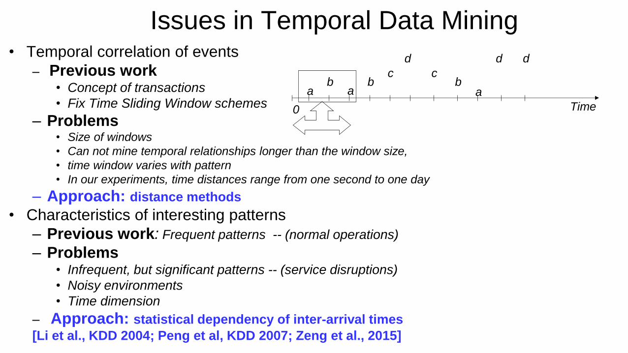
Issues in Temporal Data Mining • Temporal correlation of events
– Previous work • Concept of transactions
• Fix Time Sliding Window schemes
– Problems • Size of windows
• Can not mine temporal relationships longer than the window size,
• time window varies with pattern
• In our experiments, time distances range from one second to one day
– Approach: distance methods
• Characteristics of interesting patterns
– Previous work: Frequent patterns -- (normal operations)
– Problems • Infrequent, but significant patterns -- (service disruptions)
• Noisy environments
• Time dimension
– Approach: statistical dependency of inter-arrival times
[Li et al., KDD 2004; Peng et al, KDD 2007; Zeng et al., 2015]
0 Time
a a a b b b
c c
d d d
• History on Event Mining
• Overview of Temporal Patterns
• Mining Time Lags
– Non-parametric Methods
– Parametric Methods
• Event Summarization
• Temporal Dependency
Outline
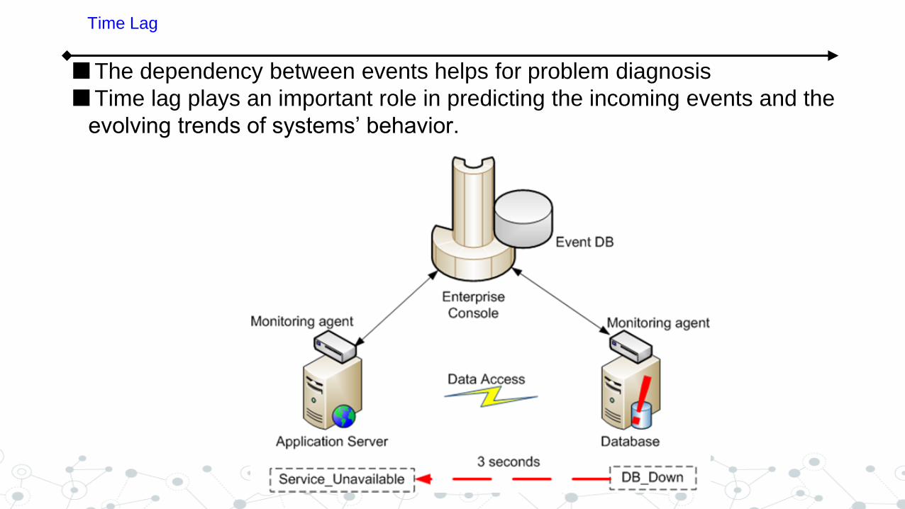
The dependency between events helps for problem diagnosis
Time lag plays an important role in predicting the incoming events and the
evolving trends of systems’ behavior.
Time Lag
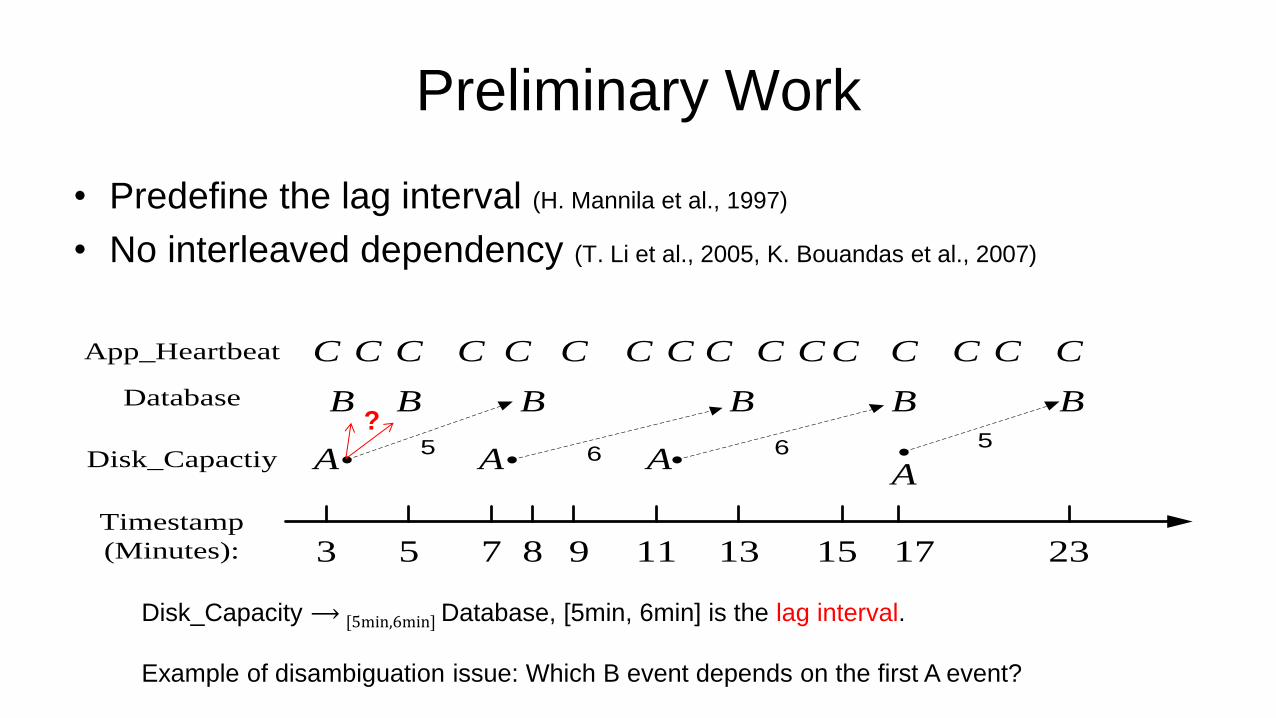
Preliminary Work
• Predefine the lag interval (H. Mannila et al., 1997)
• No interleaved dependency (T. Li et al., 2005, K. Bouandas et al., 2007)
Disk_Capacity ⟶ [5min,6min] Database, [5min, 6min] is the lag interval.
Example of disambiguation issue: Which B event depends on the first A event?
3 5 7 8 9 13 1715Timestamp
(Minutes):
Disk_Capactiy
Database
A
B B
A A
BB
665
C C CC CApp_Heartbeat C
A
B
5
23
C C C C C C C C CC
11
B?
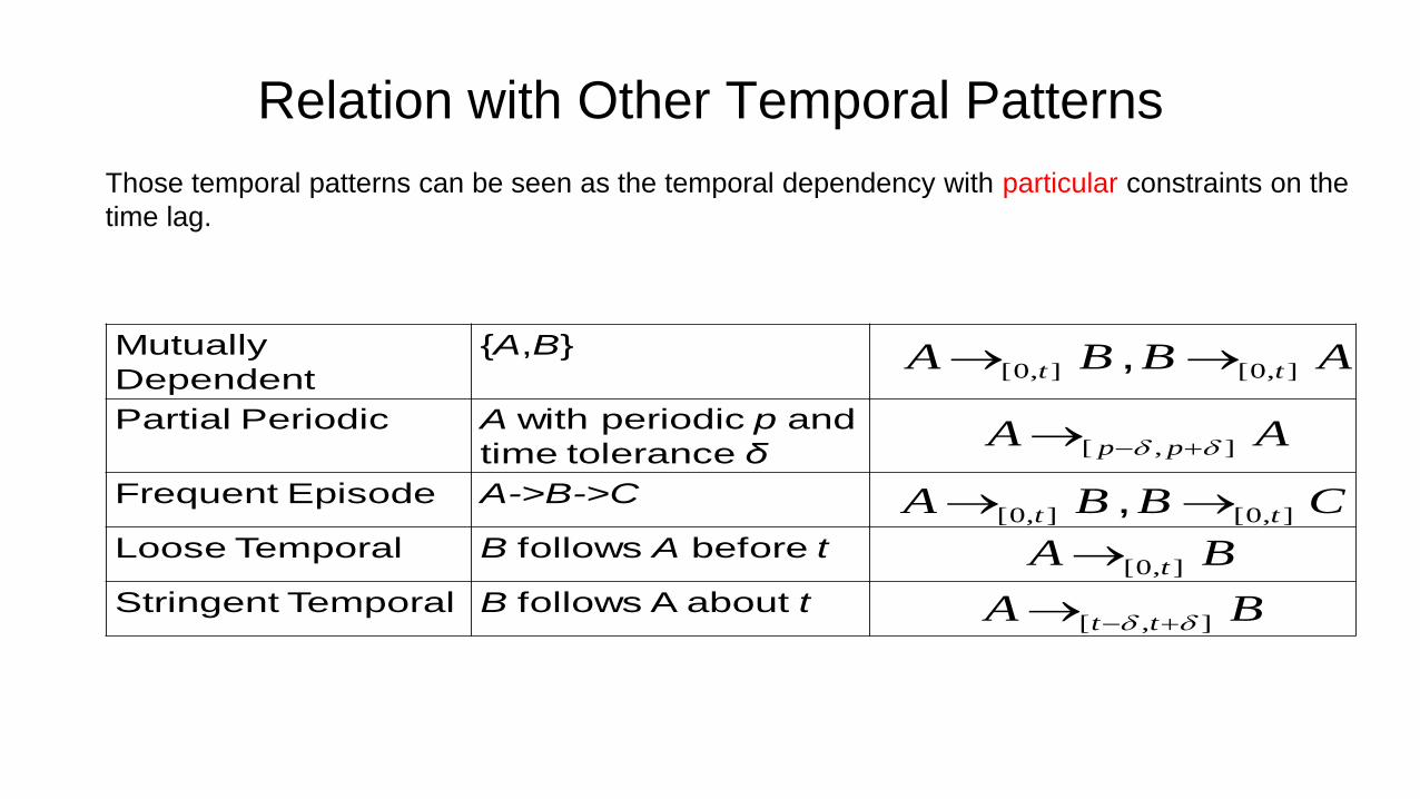
Relation with Other Temporal Patterns
Mutually
Dependent
{A,B}
Partial Periodic A with periodic p and
time tolerance δ
Frequent Episode A->B->C
Loose Temporal B follows A before t
Stringent Temporal B follows A about t
, ABBA tt ],0[],0[
AA pp ],[
, CBBA tt ],0[],0[
BA t ],0[
BA tt ],[
Those temporal patterns can be seen as the temporal dependency with particular constraints on the
time lag.
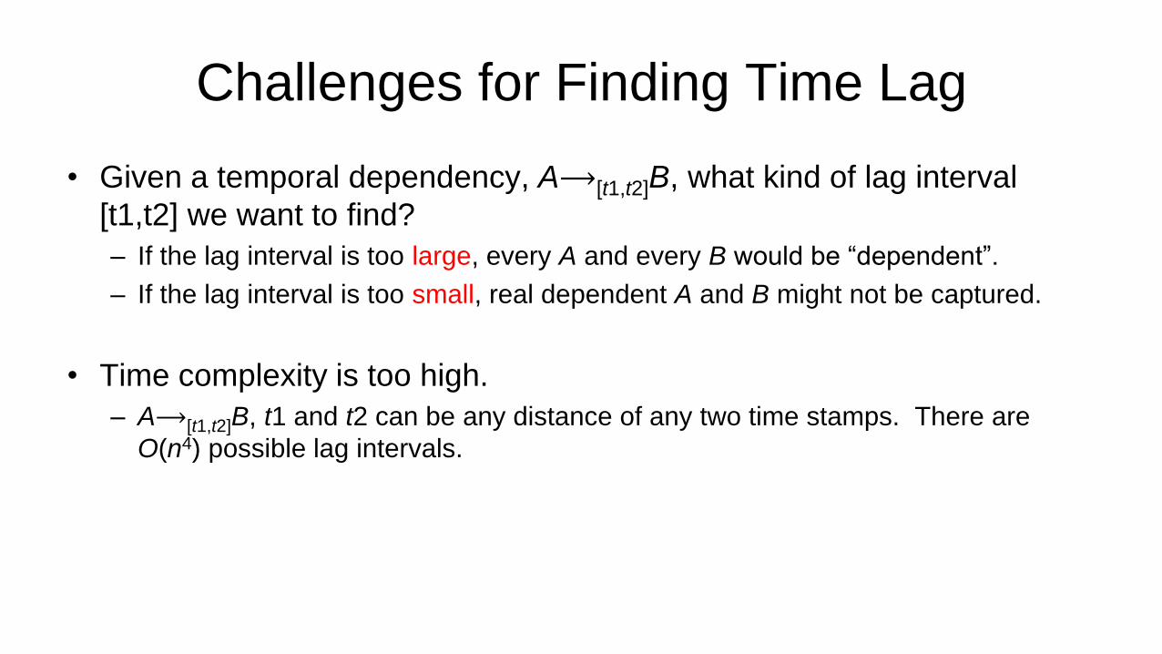
Challenges for Finding Time Lag
• Given a temporal dependency, A⟶[t1,t2]B, what kind of lag interval
[t1,t2] we want to find?
– If the lag interval is too large, every A and every B would be “dependent”.
– If the lag interval is too small, real dependent A and B might not be captured.
• Time complexity is too high.
– A⟶[t1,t2]B, t1 and t2 can be any distance of any two time stamps. There are
O(n4) possible lag intervals.
What is a Qualified Lag Interval
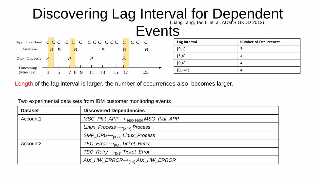
If [t1,t2] is qualified, we should observe many occurrences for A⟶[t1,t2]B.
3 5 7 8 9 13 1715Timestamp
(Minutes):
Disk_Capactiy
Database
A
B B
A A
BB
C C CC CApp_Heartbeat C
A
B
23
C C C C C C C C CC
11
B
Length of the lag interval is larger, the number of occurrences also becomes larger.
Lag Interval Number of Occurrences
[0,1] 3
[5,6] 4
[0,6] 4
[0,+∞] 4
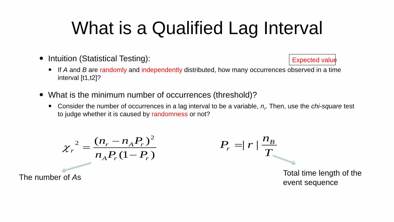
What is a Qualified Lag Interval
Intuition (Statistical Testing):
If A and B are randomly and independently distributed, how many occurrences observed in a time
interval [t1,t2]?
What is the minimum number of occurrences (threshold)?
Consider the number of occurrences in a lag interval to be a variable, nr. Then, use the chi-square test
to judge whether it is caused by randomness or not?
The number of As Total time length of the
event sequence
)1(
)( 22
rrA
rArr
PPn
Pnn
T
nrP B
r ||
Expected value
Naive Algorithm for Finding Qualified Lag
Intervals
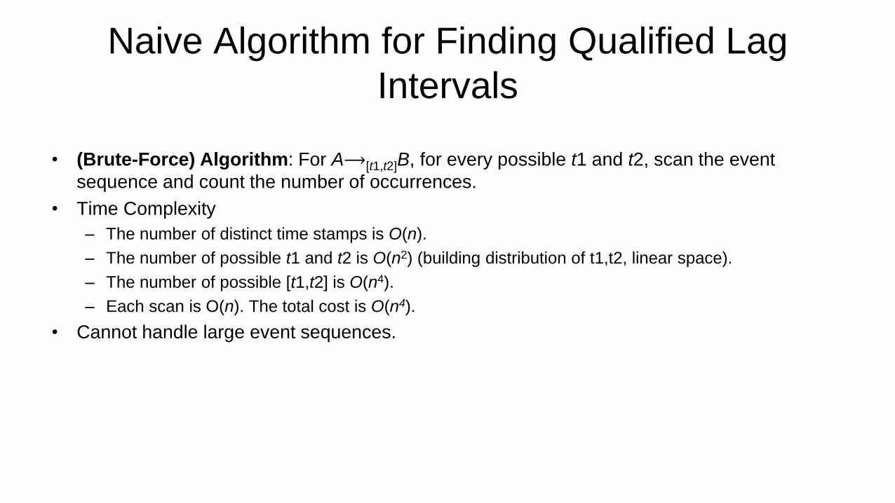
• (Brute-Force) Algorithm: For A⟶[t1,t2]B, for every possible t1 and t2, scan the event
sequence and count the number of occurrences.
• Time Complexity
– The number of distinct time stamps is O(n).
– The number of possible t1 and t2 is O(n2) (building distribution of t1,t2, linear space).
– The number of possible [t1,t2] is O(n4).
– Each scan is O(n). The total cost is O(n4).
• Cannot handle large event sequences.
Discovering Lag Interval for Dependent
Events (Liang Tang, Tao Li et. al, ACM SIGKDD 2012)
Lag Interval Number of Occurrences
[0,1] 3
[5,6] 4
[0,6] 4
[0,+∞] 4 3 5 7 8 9 13 1715
Timestamp
(Minutes):
Disk_Capactiy
Database
A
B B
A A
BB
C C CC CApp_Heartbeat C
A
B
23
C C C C C C C C CC
11
B
Length of the lag interval is larger, the number of occurrences also becomes larger.
Dataset Discovered Dependencies
Account1 MSG_Plat_APP ⟶[3600,3600] MSG_Plat_APP
Linux_Process ⟶[0,96] Process
SMP_CPU⟶[0,27] Linux_Process
Account2 TEC_Error ⟶[0,1] Ticket_Retry
TEC_Retry ⟶[0,1] Ticket_Error
AIX_HW_ERROR⟶[8,9] AIX_HW_ERROR
Two experimental data sets from IBM customer monitoring events
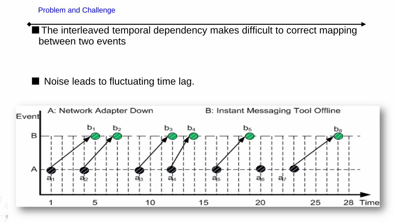
The interleaved temporal dependency makes difficult to correct mapping between two events
Noise leads to fluctuating time lag.
Problem and Challenge
A parametric model to formulate the randomness of time lags between
events. This model is capable of
providing insight into the correlation of events.
describing the distribution of time lags.
Parametric Method
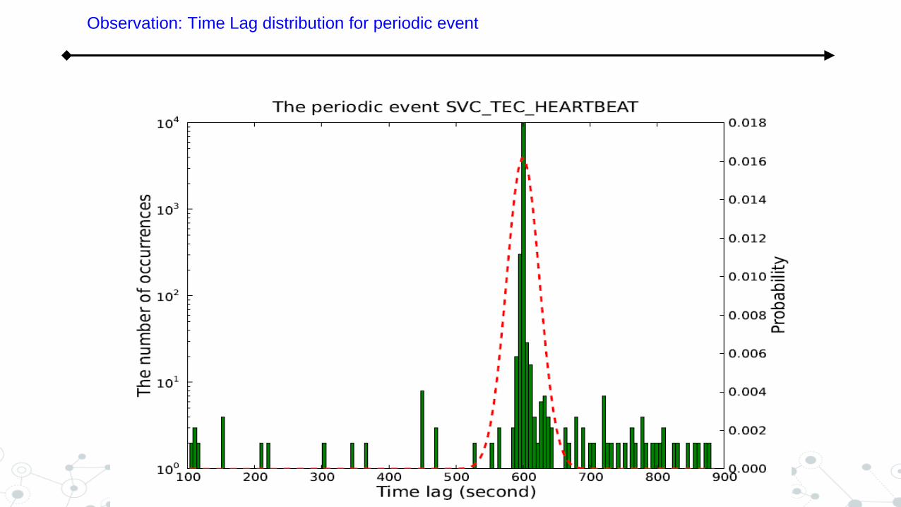
Observation: Time Lag distribution for periodic event
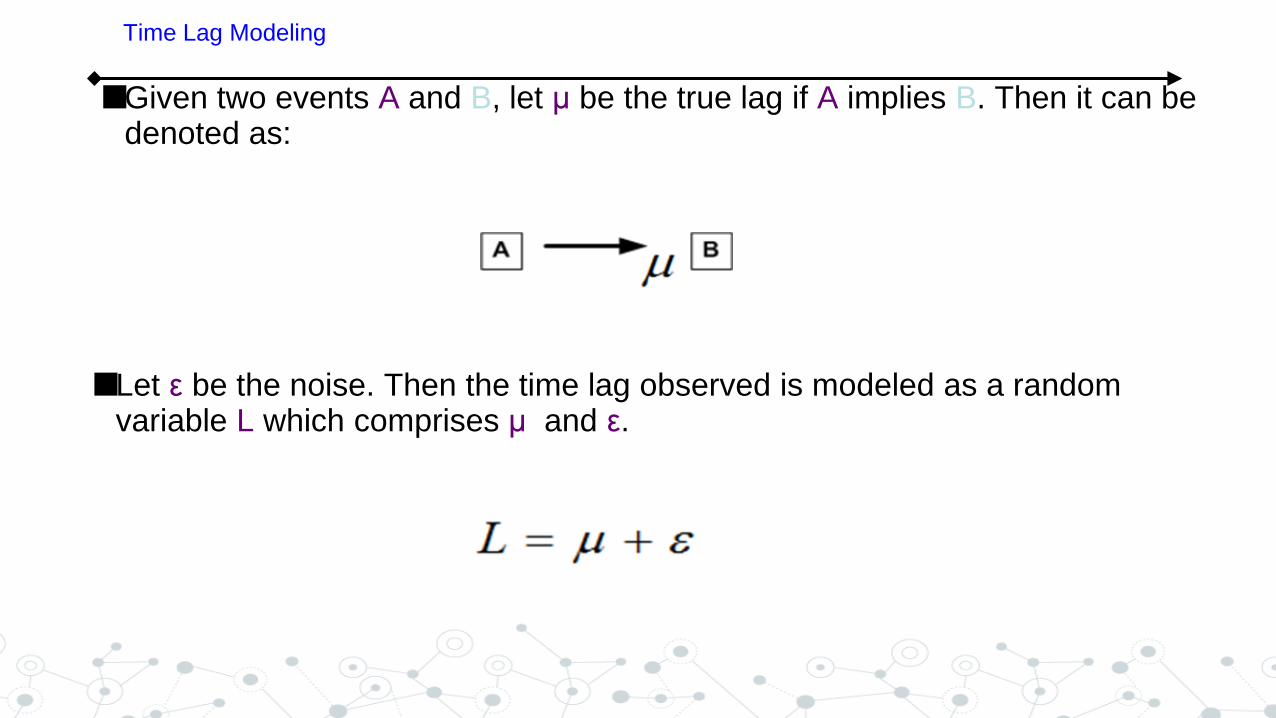
Given two events A and B, let μ be the true lag if A implies B. Then it can be denoted as:
Time Lag Modeling
Let ε be the noise. Then the time lag observed is modeled as a random variable L which comprises μ and ε.
Time Lag Modeling
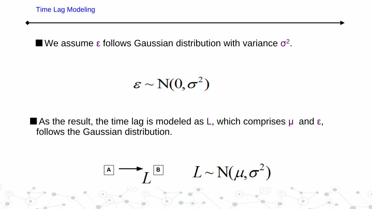
We assume ε follows Gaussian distribution with variance σ2.
As the result, the time lag is modeled as L, which comprises μ and ε, follows the Gaussian distribution.
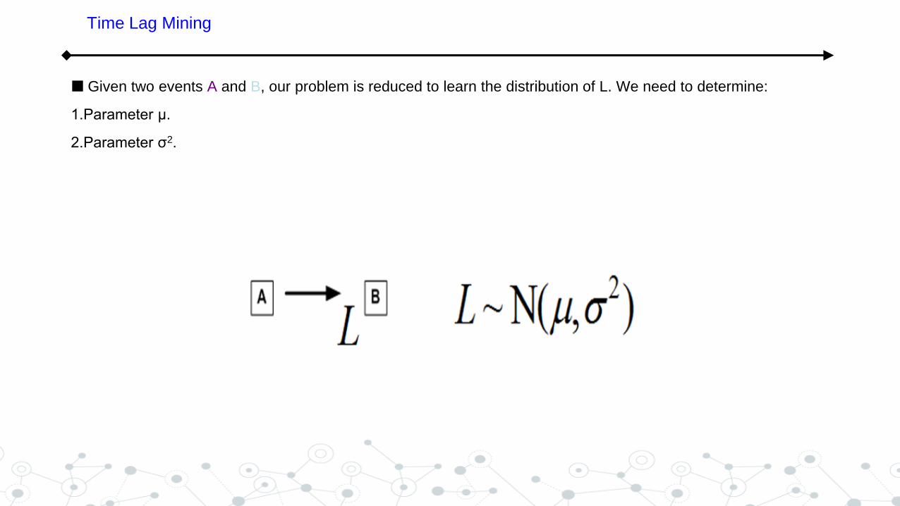
Given two events A and B, our problem is reduced to learn the distribution of L. We need to determine:
1.Parameter μ.
2.Parameter σ2.
Time Lag Mining
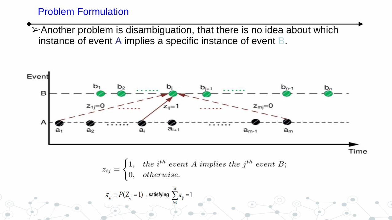
➢Another problem is disambiguation, that there is no idea about which instance of event A implies a specific instance of event B.
Problem Formulation
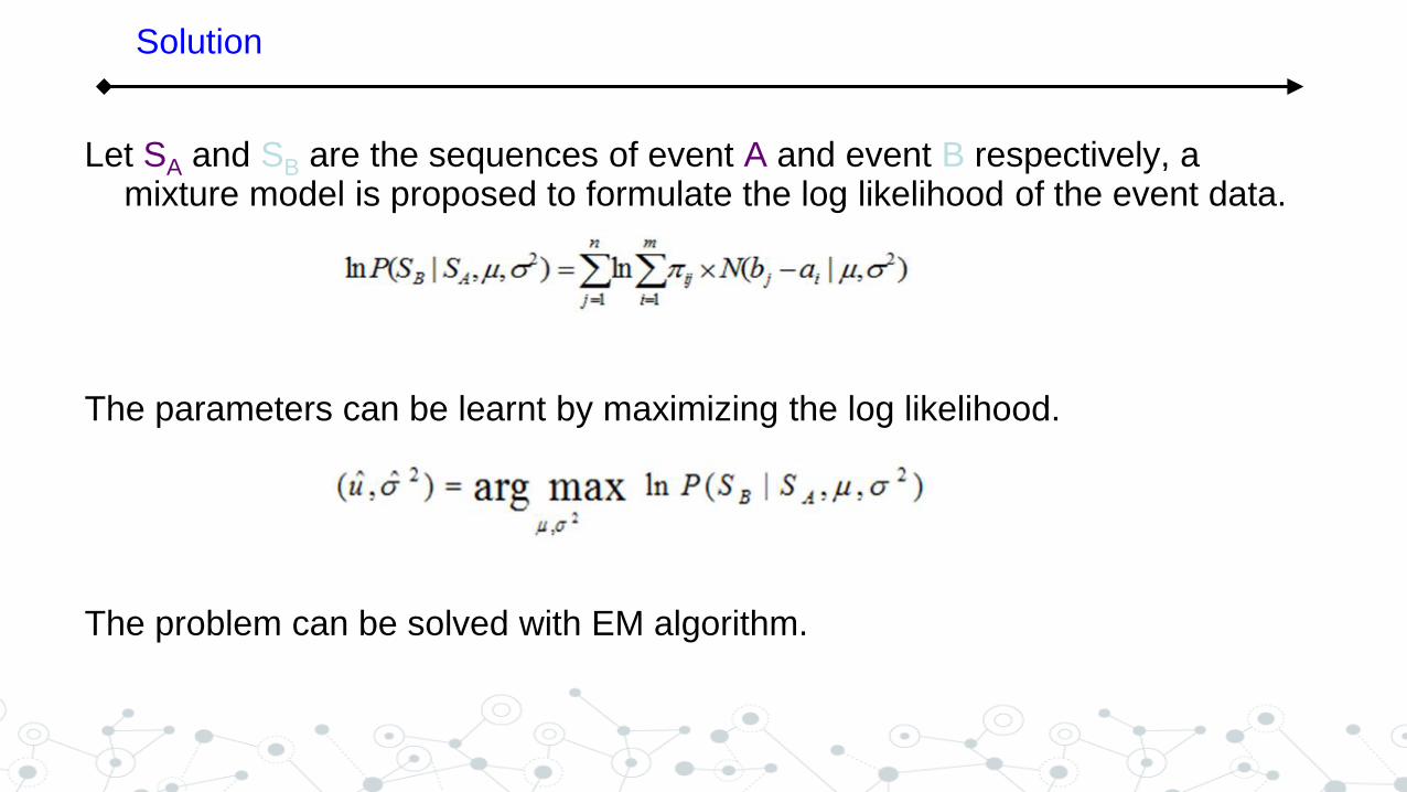
Let SA and SB are the sequences of event A and event B respectively, a mixture model is proposed to formulate the log likelihood of the event data.
The parameters can be learnt by maximizing the log likelihood.
The problem can be solved with EM algorithm.
Solution
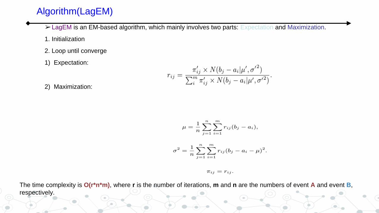
➢LagEM is an EM-based algorithm, which mainly involves two parts: Expectation and Maximization.
1. Initialization
2. Loop until converge
1) Expectation:
2) Maximization:
Algorithm(LagEM)
The time complexity is O(r*n*m), where r is the number of iterations, m and n are the numbers of event A and event B,
respectively.
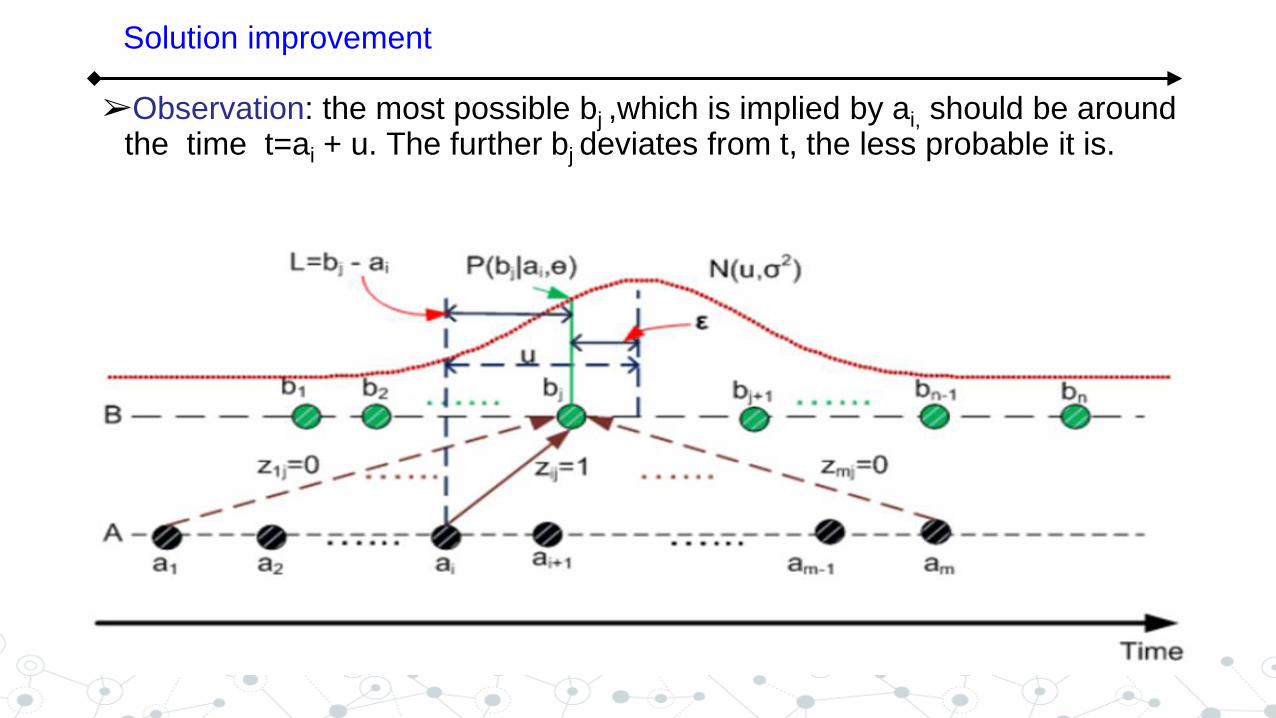
➢Observation: the most possible bj ,which is implied by ai, should be around the time t=ai + u. The further bj deviates from t, the less probable it is.
Solution improvement
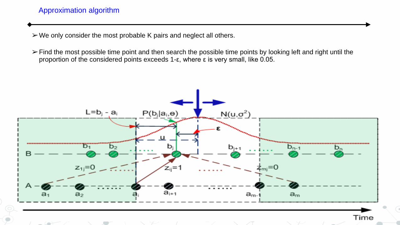
➢We only consider the most probable K pairs and neglect all others.
➢Find the most possible time point and then search the possible time points by looking left and right until the proportion of the considered points exceeds 1-ε, where ε is very small, like 0.05.
Approximation algorithm
➢ Setup
● Synthetic data: noise and true lags are incorporated into data.
● Provided with ground truth, the experiment conducted on synthetic data allows us to demonstrate the effectiveness.
● Provided with different numbers of synthetic events, it allows to illustrate the efficiency of our algorithm.
➢ Real data: data is collected from several IT outsourcing centers by IBM Tivoli monitoring system.
● It shows that temporal dependencies with time lags can be discovered by running our proposed algorithm.
● Detailed analysis demonstrates the effectiveness and usefulness of our method in practice.
Experimental Result
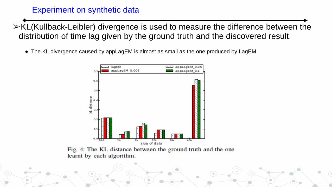
➢KL(Kullback-Leibler) divergence is used to measure the difference between the distribution of time lag given by the ground truth and the discovered result.
● The KL divergence caused by appLagEM is almost as small as the one produced by LagEM
Experiment on synthetic data
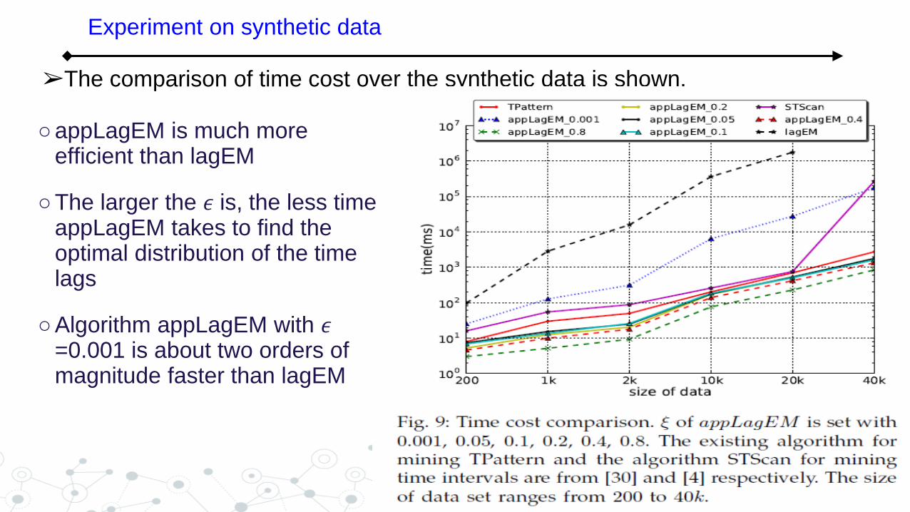
➢The comparison of time cost over the synthetic data is shown.
Experiment on synthetic data
○ appLagEM is much more efficient than lagEM
○ The larger the 𝜖 is, the less time appLagEM takes to find the optimal distribution of the time lags
○ Algorithm appLagEM with 𝜖=0.001 is about two orders of magnitude faster than lagEM
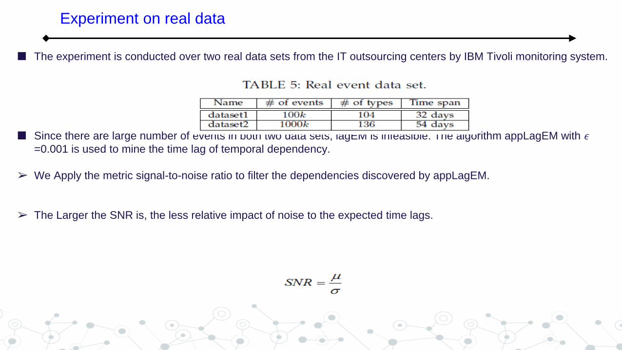
The experiment is conducted over two real data sets from the IT outsourcing centers by IBM Tivoli monitoring system.
Since there are large number of events in both two data sets, lagEM is infeasible. The algorithm appLagEM with 𝜖=0.001 is used to mine the time lag of temporal dependency.
➢ We Apply the metric signal-to-noise ratio to filter the dependencies discovered by appLagEM.
➢ The Larger the SNR is, the less relative impact of noise to the expected time lags.
Experiment on real data
Experiment on real data
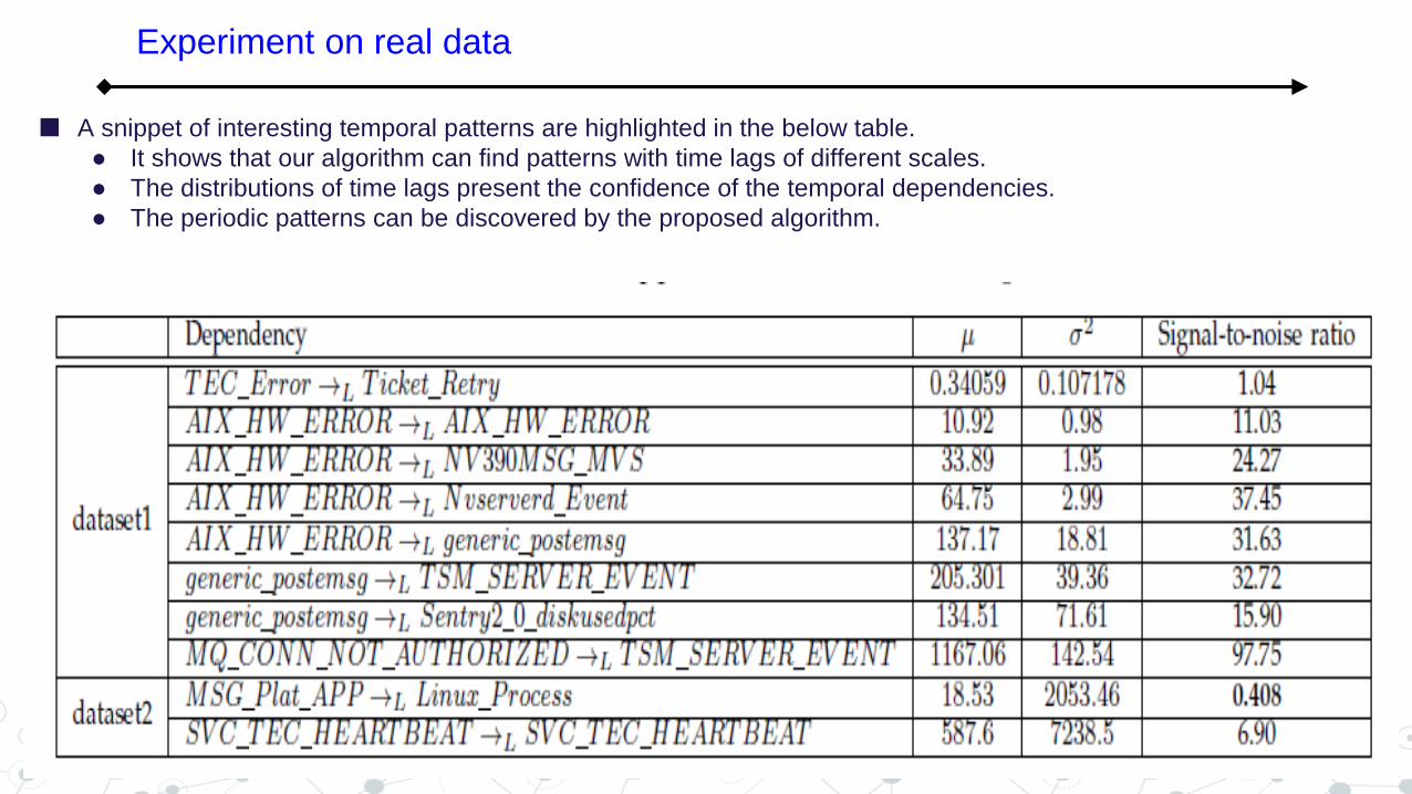
A snippet of interesting temporal patterns are highlighted in the below table.
● It shows that our algorithm can find patterns with time lags of different scales.
● The distributions of time lags present the confidence of the temporal dependencies.
● The periodic patterns can be discovered by the proposed algorithm.
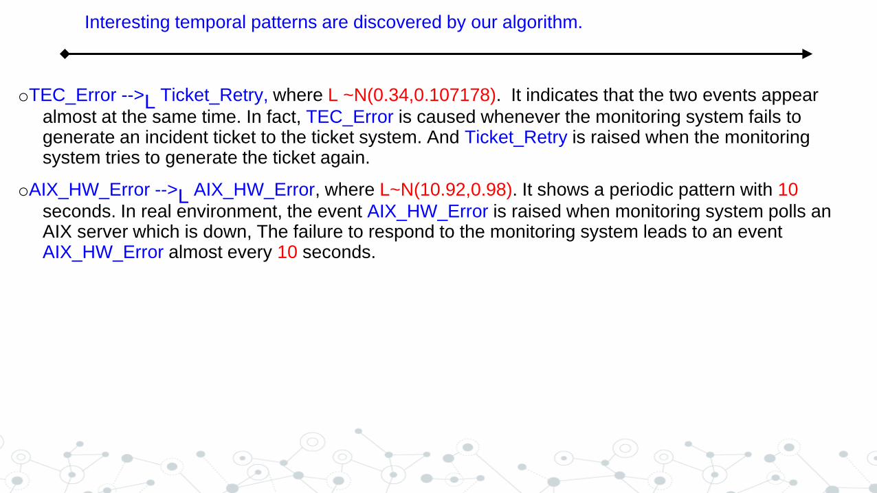
oTEC_Error -->L Ticket_Retry, where L ~N(0.34,0.107178). It indicates that the two events appear
almost at the same time. In fact, TEC_Error is caused whenever the monitoring system fails to generate an incident ticket to the ticket system. And Ticket_Retry is raised when the monitoring system tries to generate the ticket again.
oAIX_HW_Error -->L AIX_HW_Error, where L~N(10.92,0.98). It shows a periodic pattern with 10
seconds. In real environment, the event AIX_HW_Error is raised when monitoring system polls an AIX server which is down, The failure to respond to the monitoring system leads to an event AIX_HW_Error almost every 10 seconds.
Interesting temporal patterns are discovered by our algorithm.

• History on Event Mining
• Overview of Temporal Patterns
• Mining Time Lags
– Non-parametric Methods
– Parametric Methods
• Event Summarization
• Temporal Dependency
Outline
Event Summarization - Introduction
What is Event Summarization? The techniques that provide a concise interpretation of the seemingly
chaotic data, so that domain experts can take actions upon the summarized models.
Why summarize? Traditional data mining algorithms output too many patterns.
Properties of event summarization ● Brevity and accuracy
● Global data description
● Local pattern identification
● Minimize number of parameters
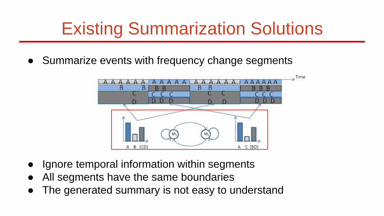
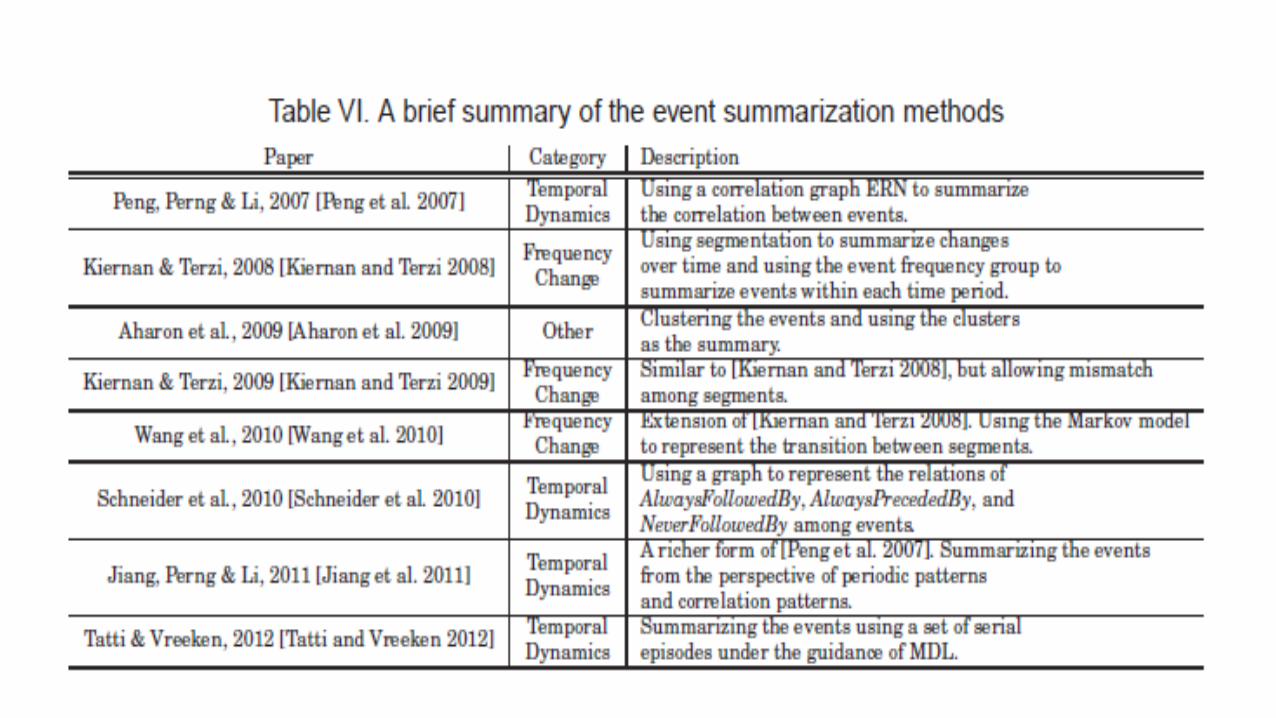
Existing Summarization Solutions
● Summarize events with frequency change segments
● Ignore temporal information within segments
● All segments have the same boundaries
● The generated summary is not easy to understand
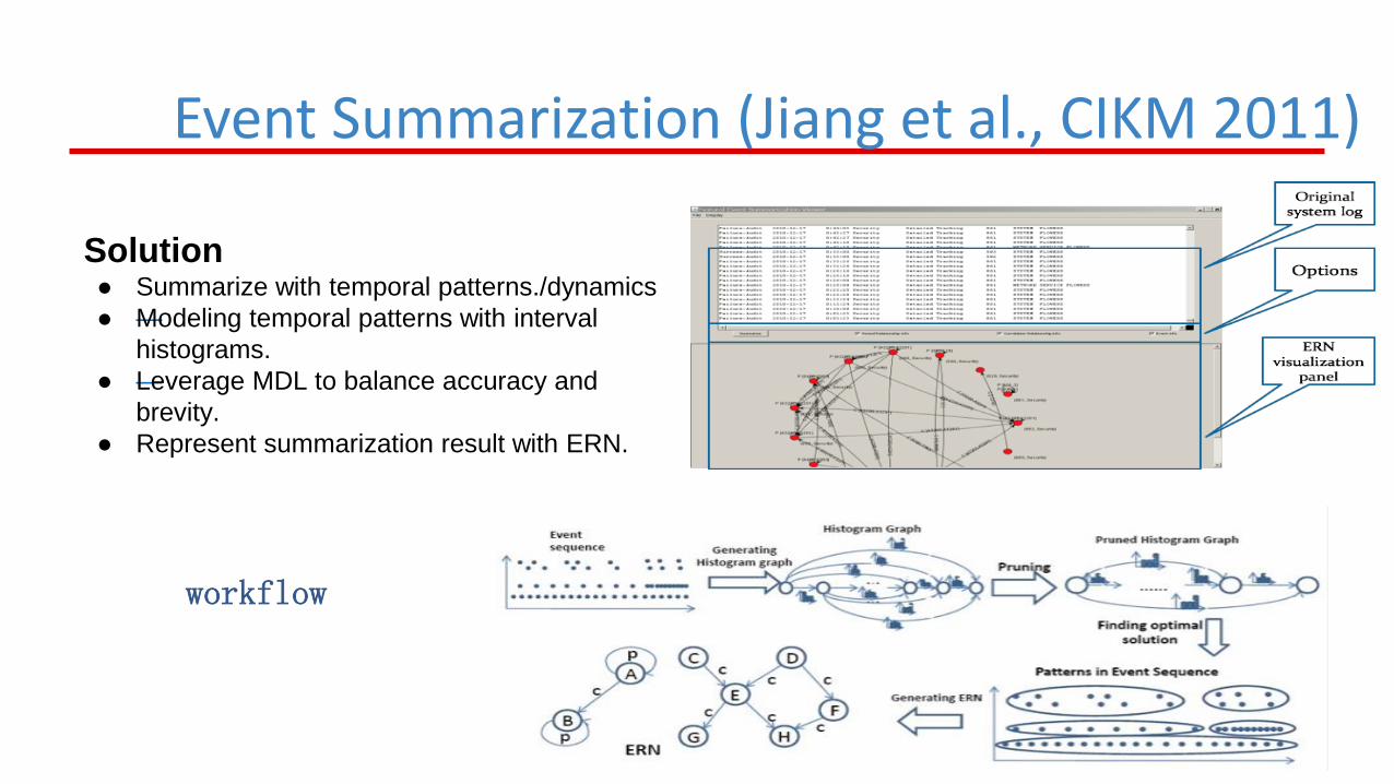
Solution ● Summarize with temporal patterns./dynamics
● —Modeling temporal patterns with interval
histograms.
● —Leverage MDL to balance accuracy and
brevity.
● Represent summarization result with ERN.
workflow
Event Summarization (Jiang et al., CIKM 2011)
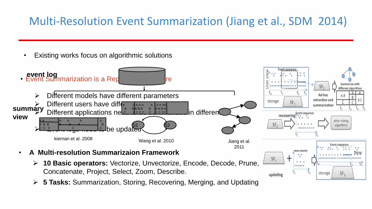
• Existing works focus on algorithmic solutions
Multi-Resolution Event Summarization (Jiang et al., SDM 2014)
• Event Summarization is a Repetitive Procedure
Different models have different parameters
Different users have different purposes
Different applications need to be summarized in different
resolutions
Event logs need to be updated
event log
summary
view
kiernan et al. 2008
A A
B B B
C C C
A A A
B B B
C
A
B
C
Jiang et al.
2011
S1 S2
A A A A A A A A AA
B B B B B B B B B B
C C C C C C C C CC
Wang et al. 2010
• A Multi-resolution Summarizaion Framework
10 Basic operators: Vectorize, Unvectorize, Encode, Decode, Prune,
Concatenate, Project, Select, Zoom, Describe.
5 Tasks: Summarization, Storing, Recovering, Merging, and Updating
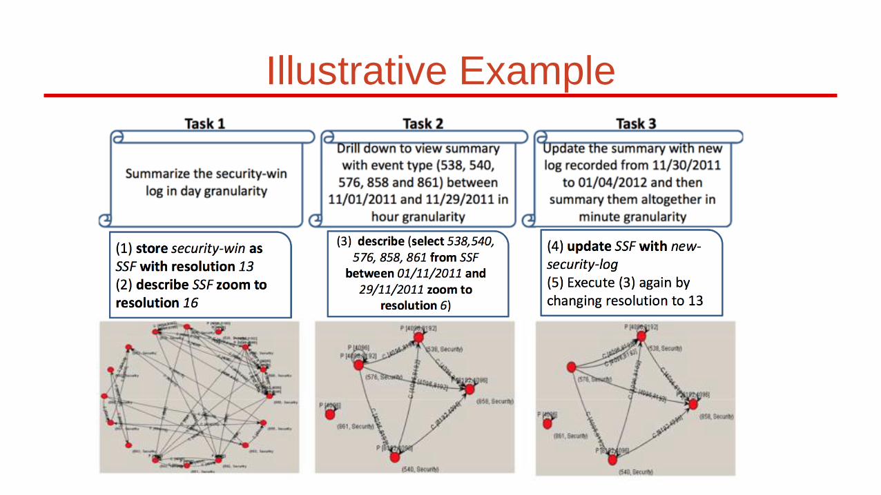
Illustrative Example
• History on Event Mining
• Overview of Temporal Patterns
• Mining Time Lags
– Non-parametric Methods
– Parametric Methods
• Event Summarization
• Temporal Dependency
Outline
➢System statistics is collected instantly as time series data.
Problem and Challenge
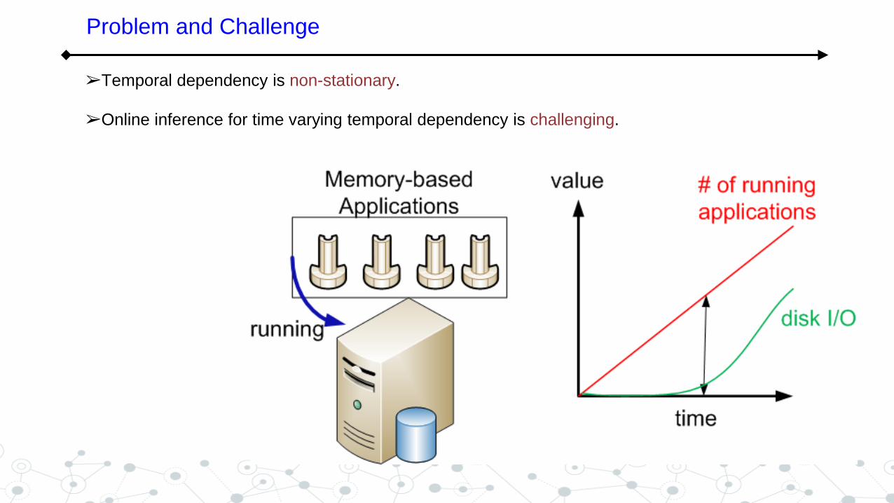
➢Temporal dependency is non-stationary.
➢Online inference for time varying temporal dependency is challenging.
Problem and Challenge
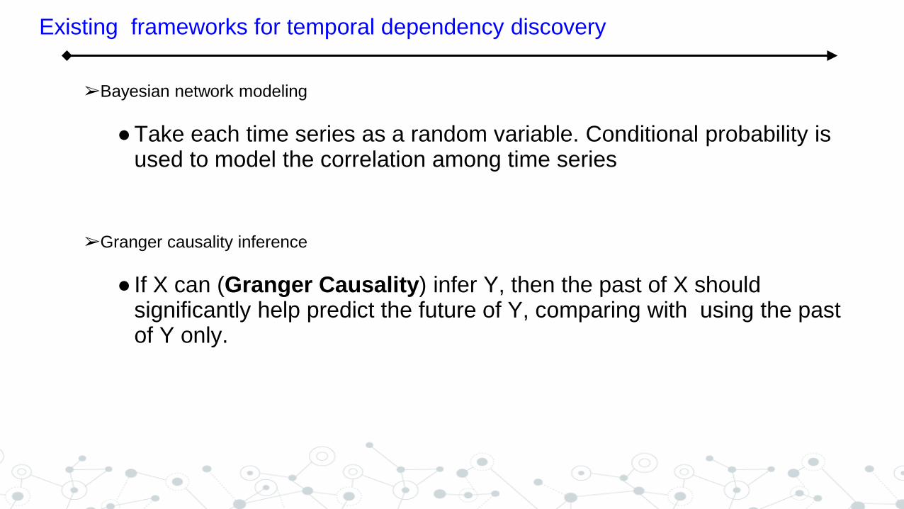
➢Bayesian network modeling
● Take each time series as a random variable. Conditional probability is used to model the correlation among time series
➢Granger causality inference
● If X can (Granger Causality) infer Y, then the past of X should significantly help predict the future of Y, comparing with using the past of Y only.
Existing frameworks for temporal dependency discovery
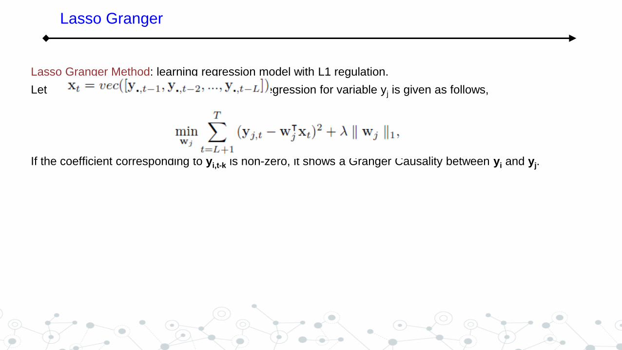
Lasso Granger
Lasso Granger Method: learning regression model with L1 regulation.
Let , the lasso regression for variable yj is given as follows,
If the coefficient corresponding to yi,t-k is non-zero, it shows a Granger Causality between yi and yj.
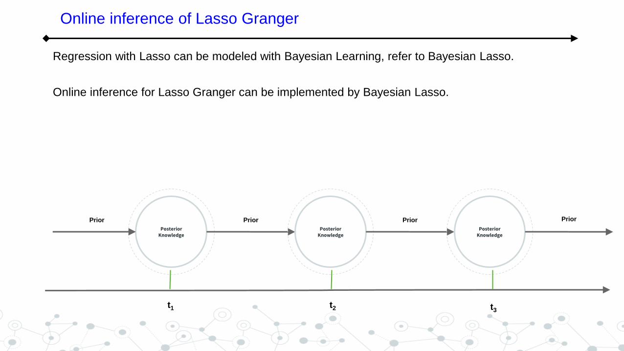
Online inference of Lasso Granger
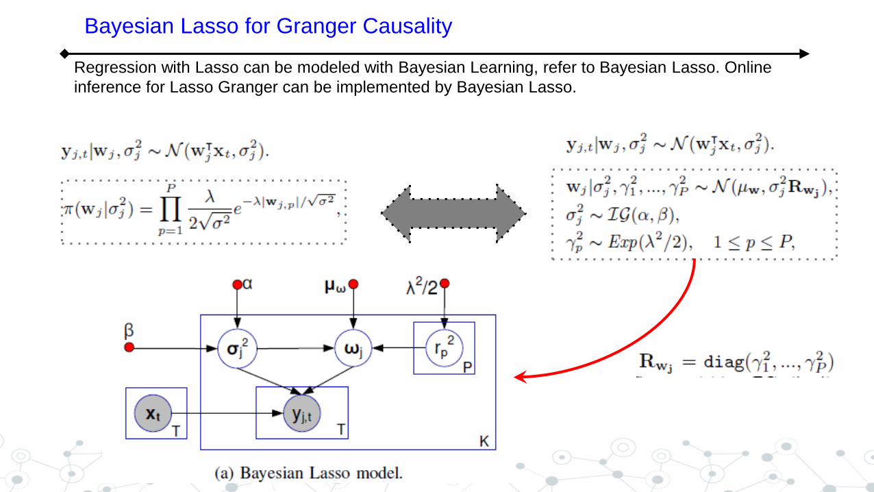
Regression with Lasso can be modeled with Bayesian Learning, refer to Bayesian Lasso.
Online inference for Lasso Granger can be implemented by Bayesian Lasso.
Posterior Knowledge
Posterior Knowledge
Prior
Posterior Knowledge
Prior Prior Prior
t1 t2 t3
Bayesian Lasso for Granger Causality
Regression with Lasso can be modeled with Bayesian Learning, refer to Bayesian Lasso. Online
inference for Lasso Granger can be implemented by Bayesian Lasso.
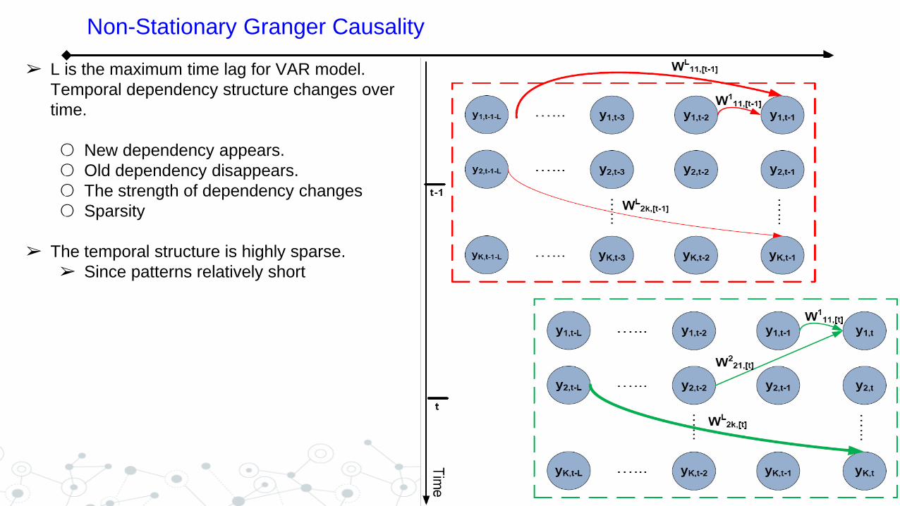
Non-Stationary Granger Causality
➢ L is the maximum time lag for VAR model.
Temporal dependency structure changes over
time.
○ New dependency appears.
○ Old dependency disappears.
○ The strength of dependency changes
○ Sparsity
➢ The temporal structure is highly sparse.
➢ Since patterns relatively short
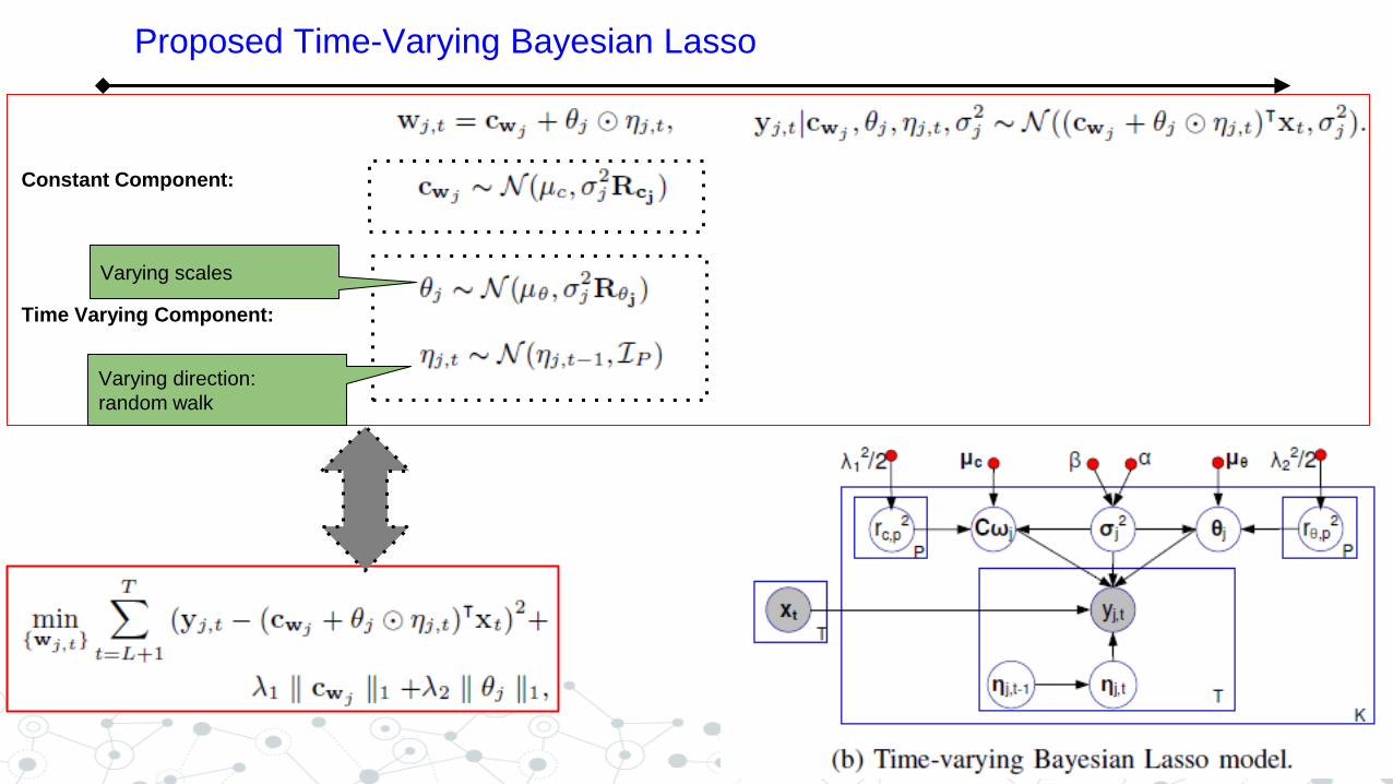
Proposed Time-Varying Bayesian Lasso
Varying scales
Varying direction:
random walk
Time Varying Component:
Constant Component:
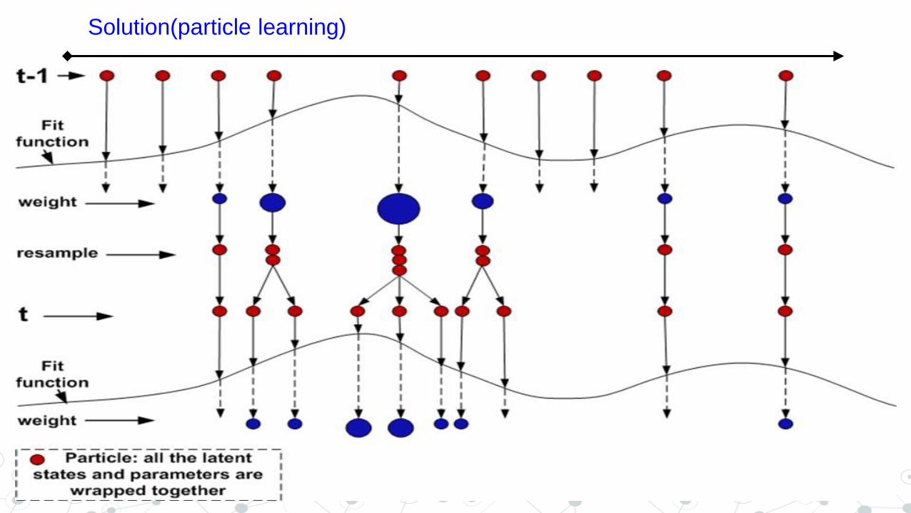
Solution(particle learning)
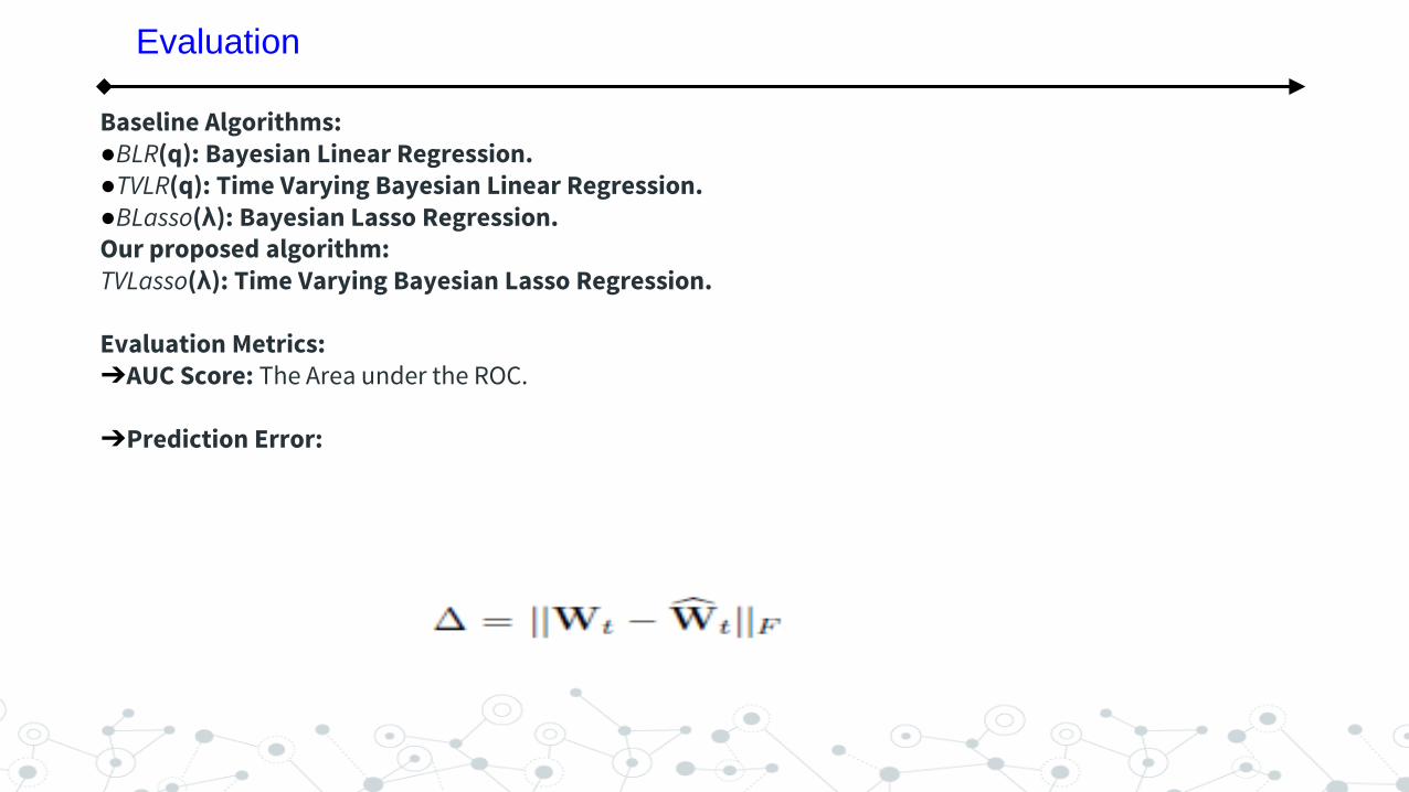
Baseline Algorithms: ●BLR(q): Bayesian Linear Regression. ●TVLR(q): Time Varying Bayesian Linear Regression. ●BLasso(λ): Bayesian Lasso Regression. Our proposed algorithm: TVLasso(λ): Time Varying Bayesian Lasso Regression. Evaluation Metrics: ➔AUC Score: The Area under the ROC. ➔Prediction Error:
Evaluation
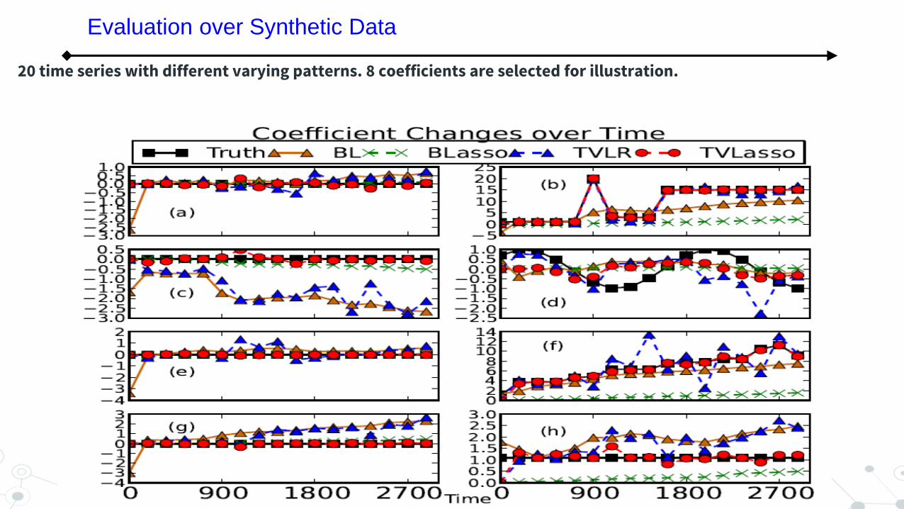
20 time series with different varying patterns. 8 coefficients are selected for illustration.
Evaluation over Synthetic Data
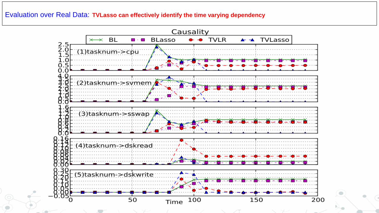
Evaluation over Real Data: TVLasso can effectively identify the time varying dependency
Introduction and Overview
Contents
1
Event Generation and System Monitoring
2
Pattern Discovery and Summarization
3
Conclusions 5
Mining with Events and Tickets 4
• Ticket Classification
• Ticket Resolution Recommendation
• Ticket Analysis (Knowledge Extraction)
Outline
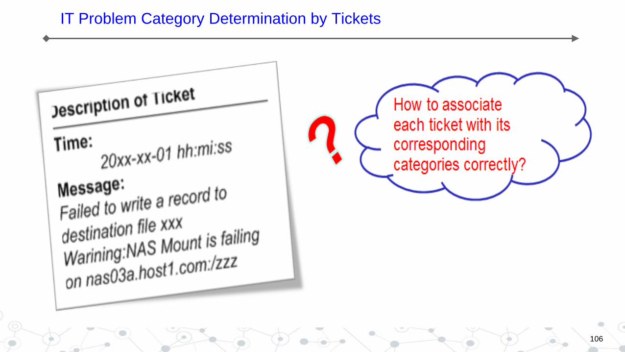
106
IT Problem Category Determination by Tickets
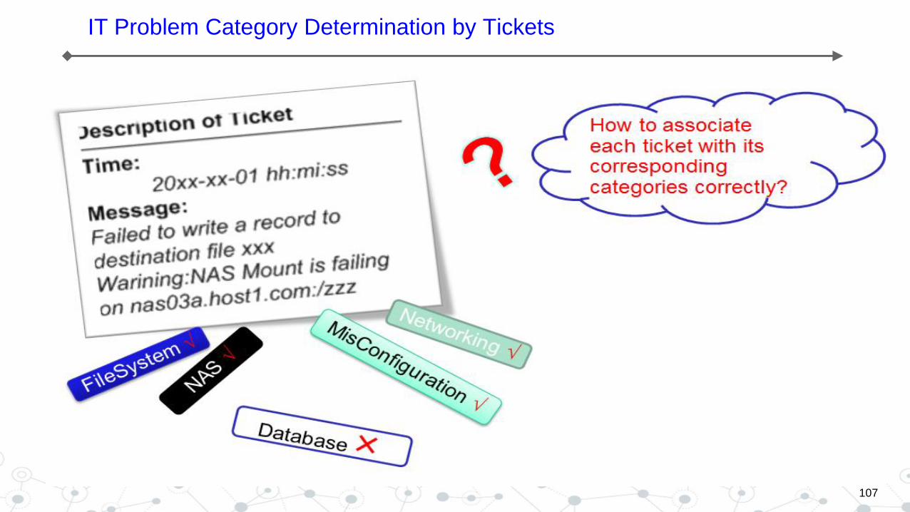
107
IT Problem Category Determination by Tickets
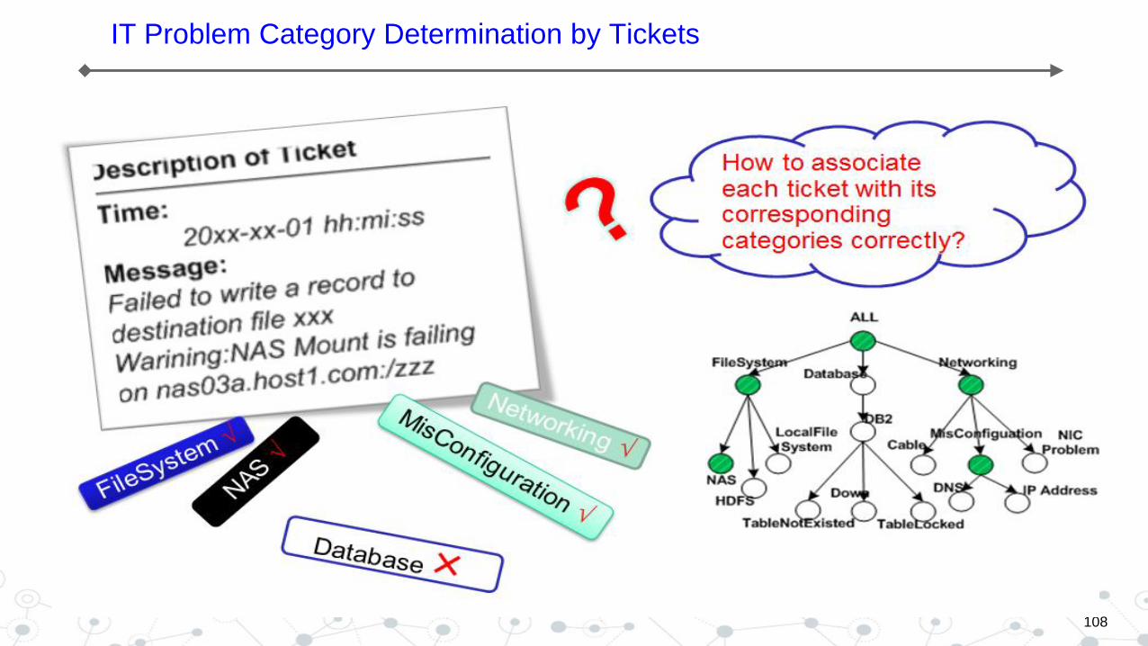
108
IT Problem Category Determination by Tickets
➢Text classification (Without considering multi-label and label hierarchy)
● SVM,CART, KNN, Rule-based classification, logistic regression
➢Multi-label classification algorithm(Without considering label hierarchy)
● Problem transformation based approach
● Algorithm adaption based approach
➢Hierarchical multi-label classification algorithm
● Recursively split the training data(Overfitting)
● Hierarchical consistency is guaranteed by post-processing(Our method belongs to this category)
109
Related Work
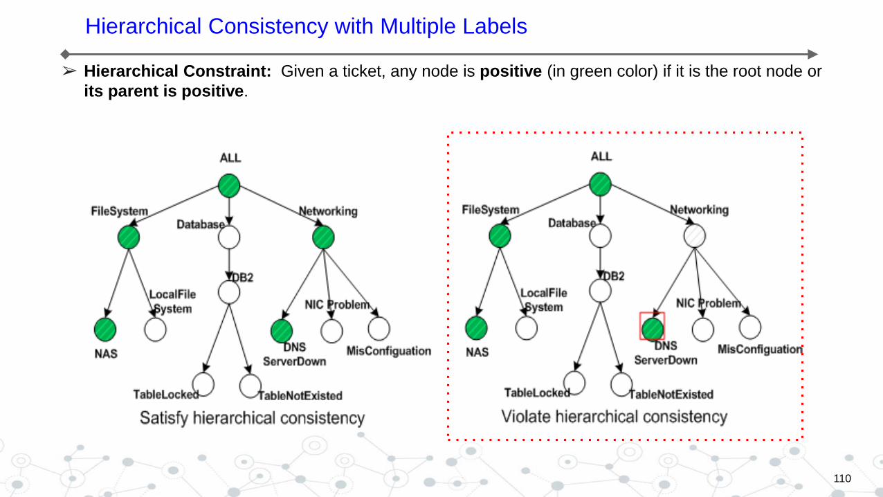
➢ Hierarchical Constraint: Given a ticket, any node is positive (in green color) if it is the root node or
its parent is positive.
110
Hierarchical Consistency with Multiple Labels
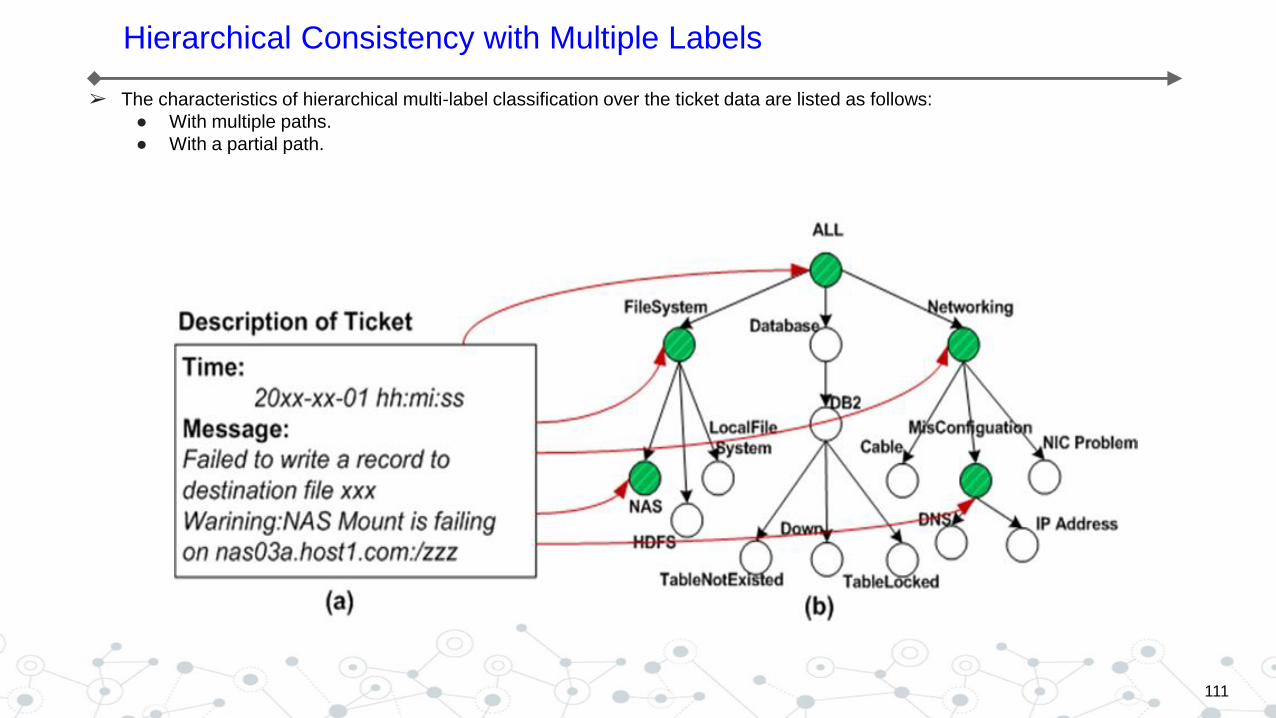
➢ The characteristics of hierarchical multi-label classification over the ticket data are listed as follows:
● With multiple paths.
● With a partial path.
111
Hierarchical Consistency with Multiple Labels
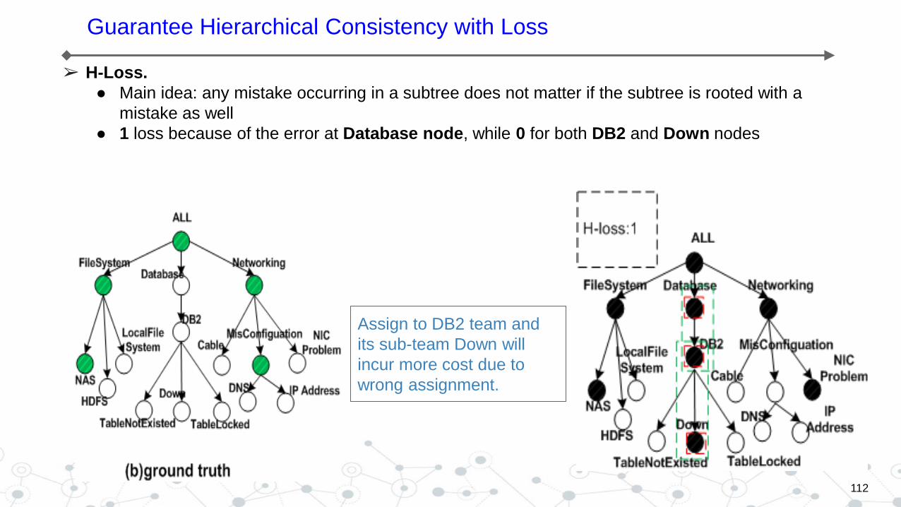
➢ H-Loss.
● Main idea: any mistake occurring in a subtree does not matter if the subtree is rooted with a
mistake as well
● 1 loss because of the error at Database node, while 0 for both DB2 and Down nodes
112
Guarantee Hierarchical Consistency with Loss
Assign to DB2 team and
its sub-team Down will
incur more cost due to
wrong assignment.
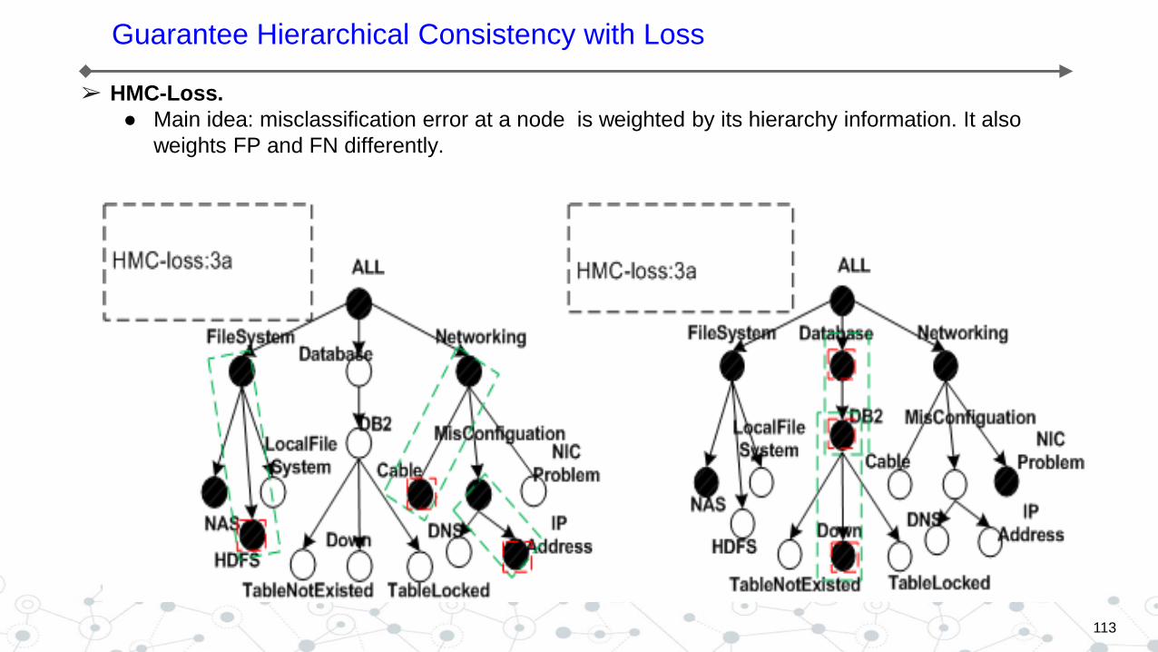
➢ HMC-Loss.
● Main idea: misclassification error at a node is weighted by its hierarchy information. It also
weights FP and FN differently.
113
Guarantee Hierarchical Consistency with Loss
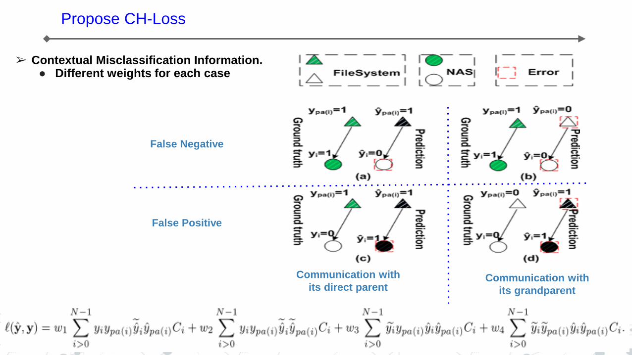
➢ Contextual Misclassification Information. ● Different weights for each case
114
Propose CH-Loss
Communication with
its direct parent Communication with
its grandparent
False Negative
False Positive
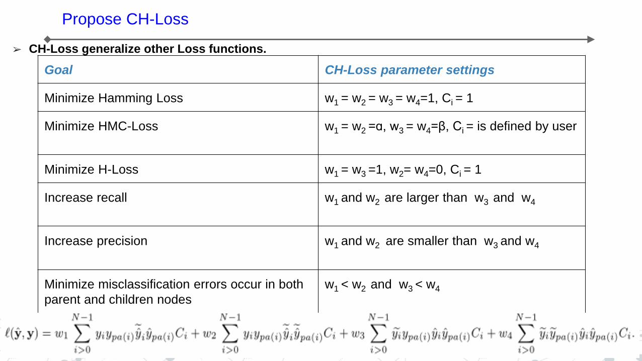
➢ CH-Loss generalize other Loss functions.
115
Propose CH-Loss
Goal CH-Loss parameter settings
Minimize Hamming Loss w1 = w2 = w3 = w4=1, Ci = 1
Minimize HMC-Loss w1 = w2 =ɑ, w3 = w4=β, Ci = is defined by user
Minimize H-Loss w1 = w3 =1, w2= w4=0, Ci = 1
Increase recall w1 and w2 are larger than w3 and w4
Increase precision w1 and w2 are smaller than w3 and w4
Minimize misclassification errors occur in both
parent and children nodes
w1 < w2 and w3 < w4
116
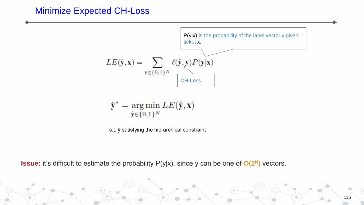
Minimize Expected CH-Loss
Issue: it’s difficult to estimate the probability P(y|x), since y can be one of O(2N) vectors.
P(y|x) is the probability of the label vector y given
ticket x.
CH-Loss
s.t. ŷ satisfying the hierarchical constraint
117
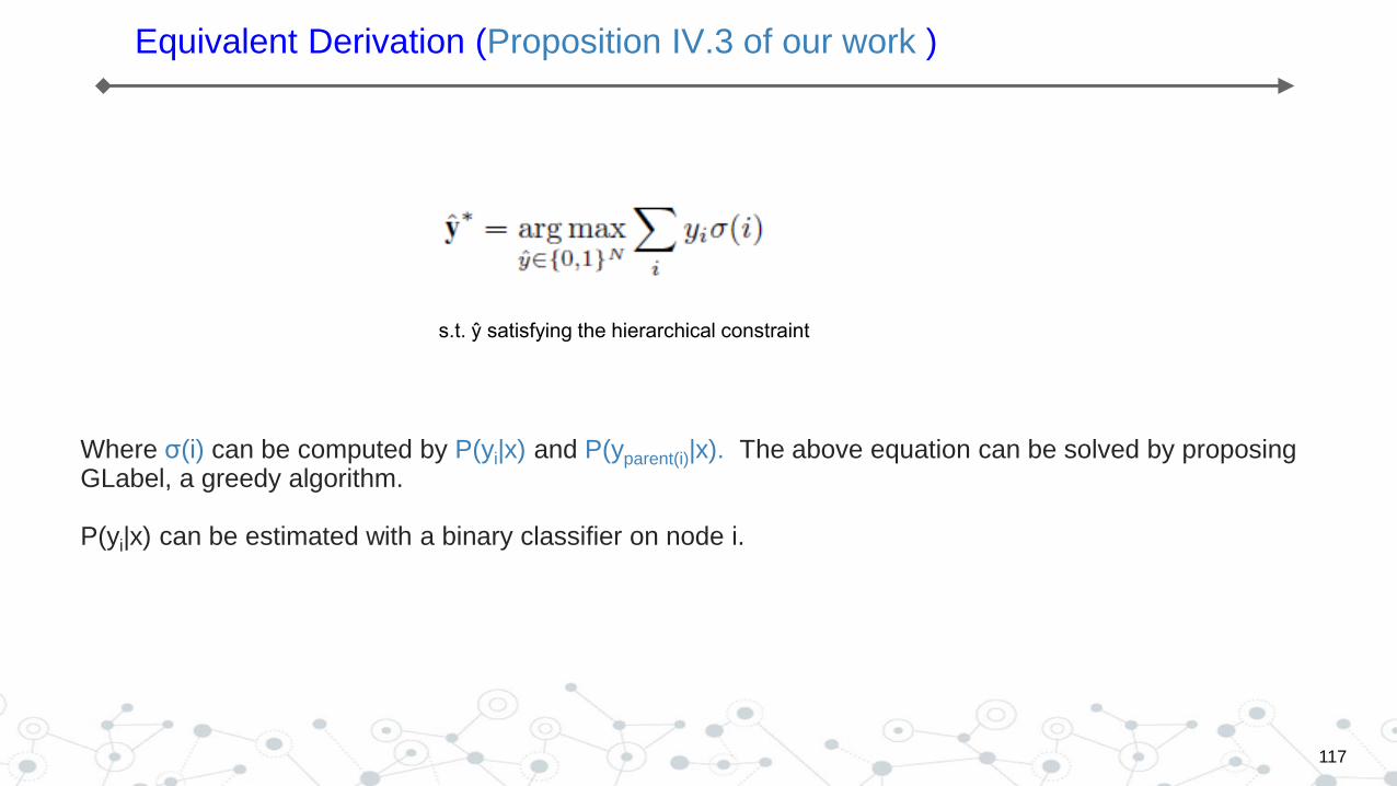
Equivalent Derivation (Proposition IV.3 of our work )
Where σ(i) can be computed by P(yi|x) and P(yparent(i)|x). The above equation can be solved by proposing GLabel, a greedy algorithm. P(yi|x) can be estimated with a binary classifier on node i.
s.t. ŷ satisfying the hierarchical constraint
118
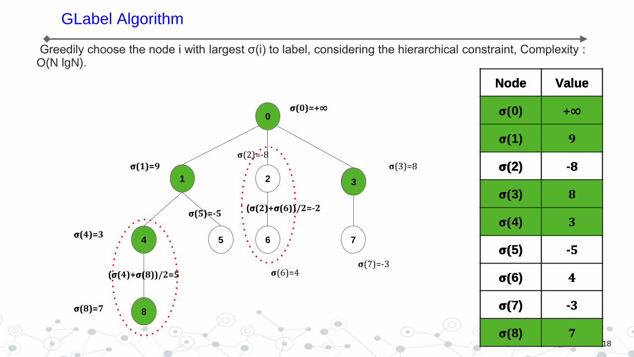
GLabel Algorithm
Greedily choose the node i with largest σ(i) to label, considering the hierarchical constraint, Complexity : O(N lgN).
0
3
8
4 6 5 7
1 2
𝛔(0)=+∞
Node Value
𝛔(0) +∞
𝛔(1) 9
𝛔(2) -8
𝛔(3) 8
𝛔(4) 3
𝛔(5) -5
𝛔(6) 4
𝛔(7) -3
𝛔(8) 7
1 3
𝛔(1)=9 𝛔(3)=8
𝛔(8)=7
𝛔(4)=3
(𝛔(4)+𝛔(8))/2=5
4
8
𝛔(6)=4
(𝛔(2)+𝛔(6))/2=-2
𝛔(2)=-8
𝛔(7)=-3
𝛔(5)=-5
Node Value
𝛔(0) +∞
𝛔(1) 9
𝛔(2) -8
𝛔(3) 8
𝛔(4) 3
𝛔(5) -5
𝛔(6) 4
𝛔(7) -3
𝛔(8) 7
Node Value
𝛔(0) +∞
𝛔(1) 9
𝛔(2) -8
𝛔(3) 8
𝛔(4) 3
𝛔(5) -5
𝛔(6) 4
𝛔(7) -3
𝛔(8) 7
Node Value
𝛔(0) +∞
𝛔(1) 9
𝛔(2) -8
𝛔(3) 8
𝛔(4) 3
𝛔(5) -5
𝛔(6) 4
𝛔(7) -3
𝛔(8) 7
1. 23,000 tickets are collected from the real IT environment. 1. 20,000 tickets are randomly selected for training data 1. The remaining 3,000 tickets are used for testing.
119
Experiment
120
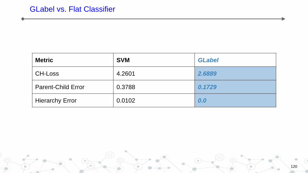
GLabel vs. Flat Classifier
Metric SVM GLabel
CH-Loss 4.2601 2.6889
Parent-Child Error 0.3788 0.1729
Hierarchy Error 0.0102 0.0
121
The state-of-the-art algorithm
1. CSSA , which requires the number of labels for each ticket
1. HIROM, which requires the maximum number of labels for all the tickets
The GLabel algorithm is capable of minimizing the loss automatically.
122
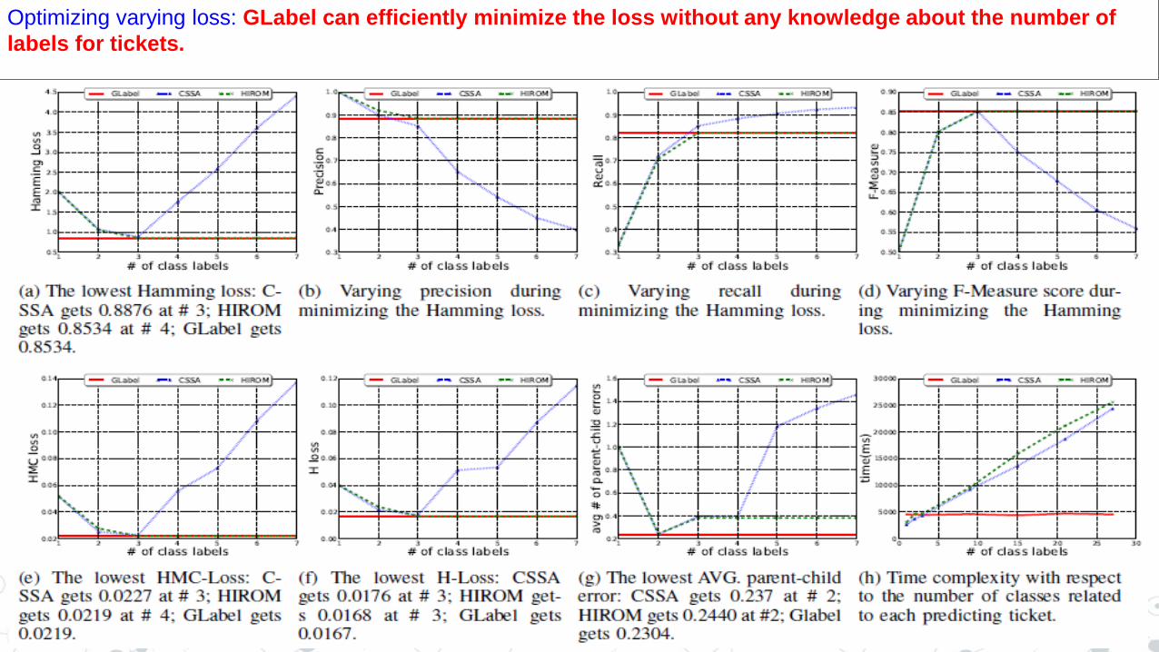
,GLabel can efficiently minimize the loss without any knowledge about the number of labels for tickets. Optimizing varying loss: GLabel can efficiently minimize the loss without any knowledge about the number of
labels for tickets.
123
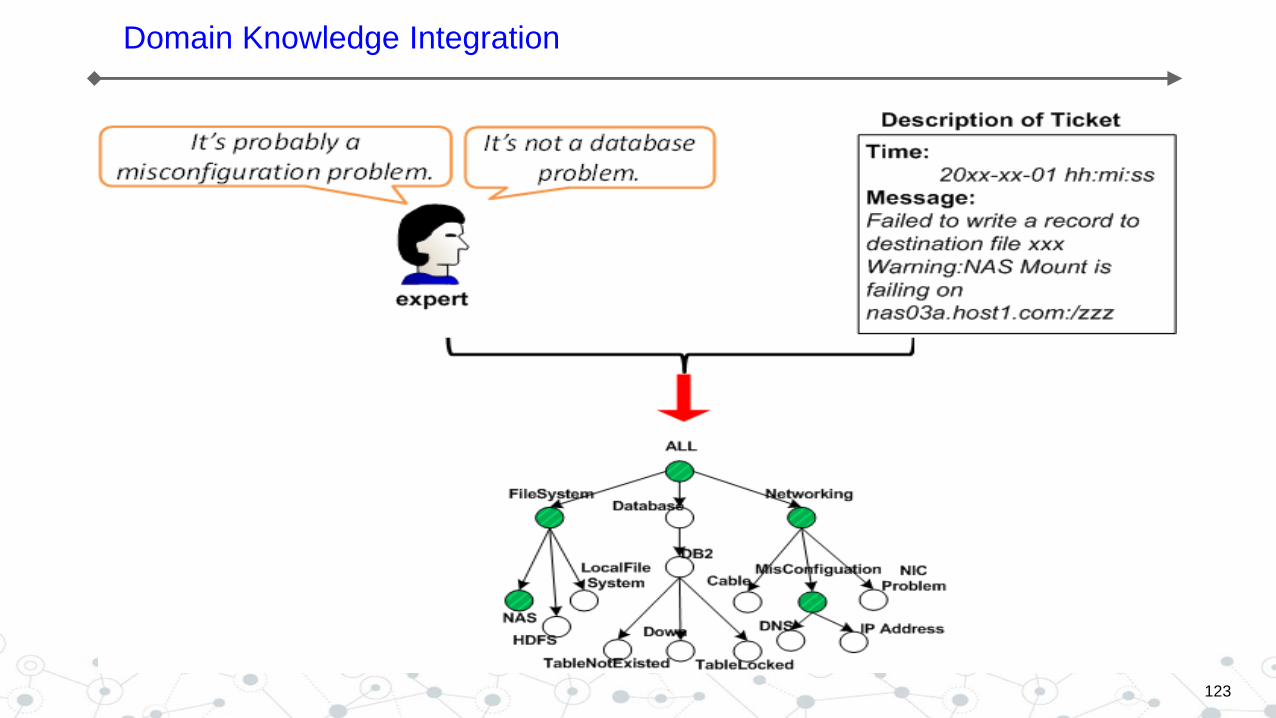
Domain Knowledge Integration
124
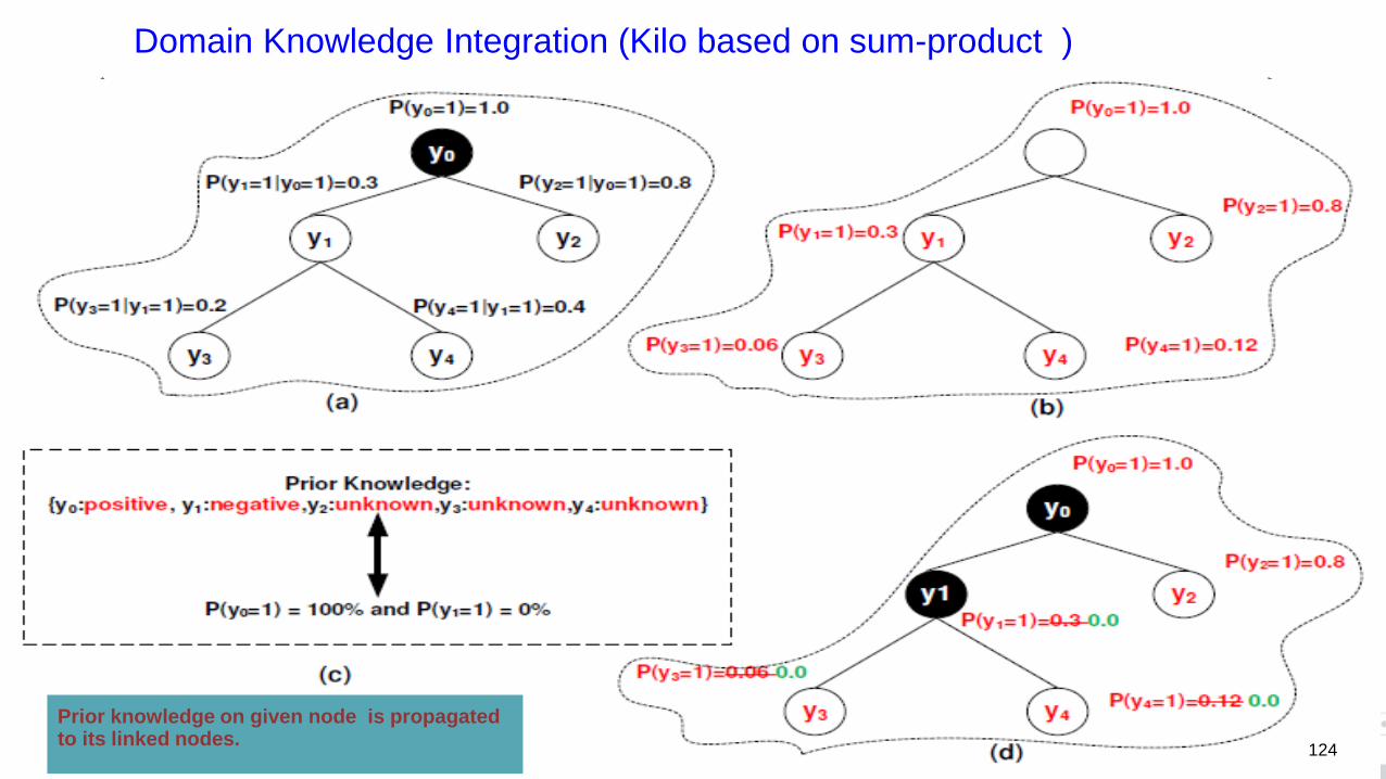
Domain Knowledge Integration (Kilo based on sum-product )
Prior knowledge on given node is propagated to its linked nodes.
125
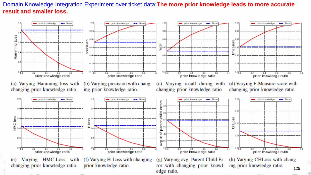
Domain Knowledge Integration Experiment over ticket data:The more prior knowledge leads to more accurate
result and smaller loss.
• Ticket Classification
• Ticket Resolution Recommendation
• Ticket Analysis (Knowledge Extraction)
Outline
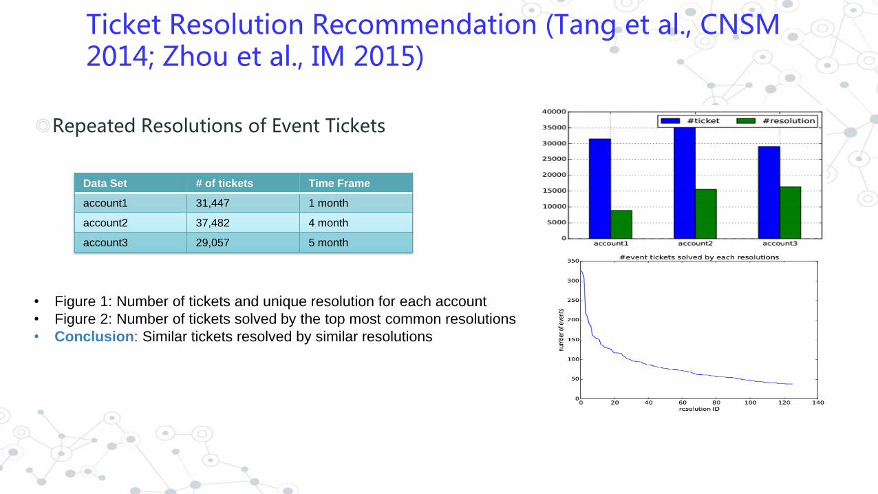
Ticket Resolution Recommendation (Tang et al., CNSM 2014; Zhou et al., IM 2015)
◎Repeated Resolutions of Event Tickets
• Figure 1: Number of tickets and unique resolution for each account
• Figure 2: Number of tickets solved by the top most common resolutions
• Conclusion: Similar tickets resolved by similar resolutions
Data Set # of tickets Time Frame
account1 31,447 1 month
account2 37,482 4 month
account3 29,057 5 month
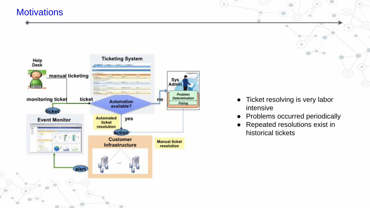
Motivations
● Ticket resolving is very labor
intensive
● Problems occurred periodically
● Repeated resolutions exist in
historical tickets
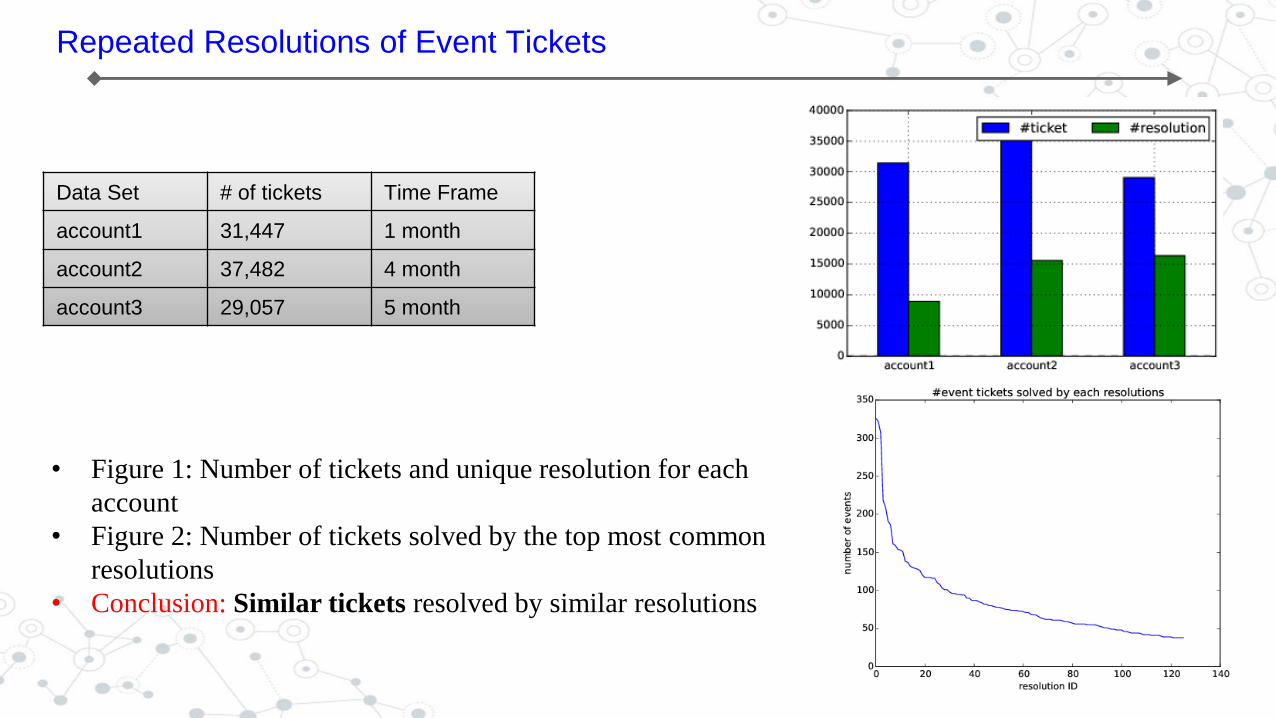
Repeated Resolutions of Event Tickets
Data Set # of tickets Time Frame
account1 31,447 1 month
account2 37,482 4 month
account3 29,057 5 month
• Figure 1: Number of tickets and unique resolution for each
account
• Figure 2: Number of tickets solved by the top most common
resolutions
• Conclusion: Similar tickets resolved by similar resolutions
Related Work
• User-based Recommendation Algorithms
• Item-based Recommendation Algorithms
• Constraint-based Recommender Systems
• Multiple Objective Optimization…
Existing Solution
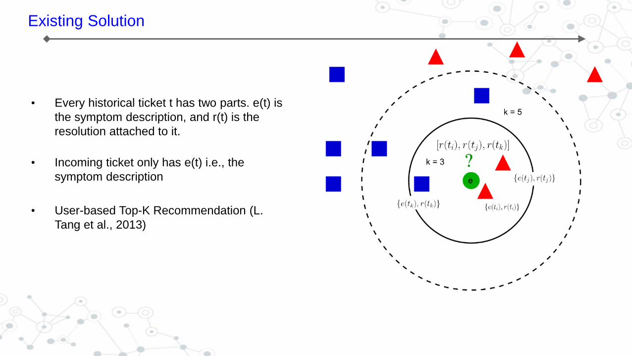
• Every historical ticket t has two parts. e(t) is
the symptom description, and r(t) is the
resolution attached to it.
• Incoming ticket only has e(t) i.e., the
symptom description
• User-based Top-K Recommendation (L.
Tang et al., 2013)
Challenges
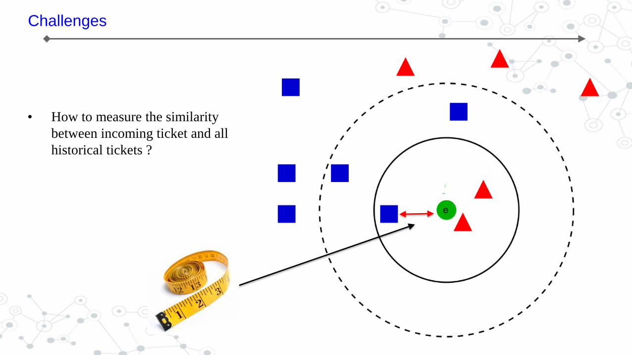
• How to measure the similarity
between incoming ticket and all
historical tickets ?
Challenges
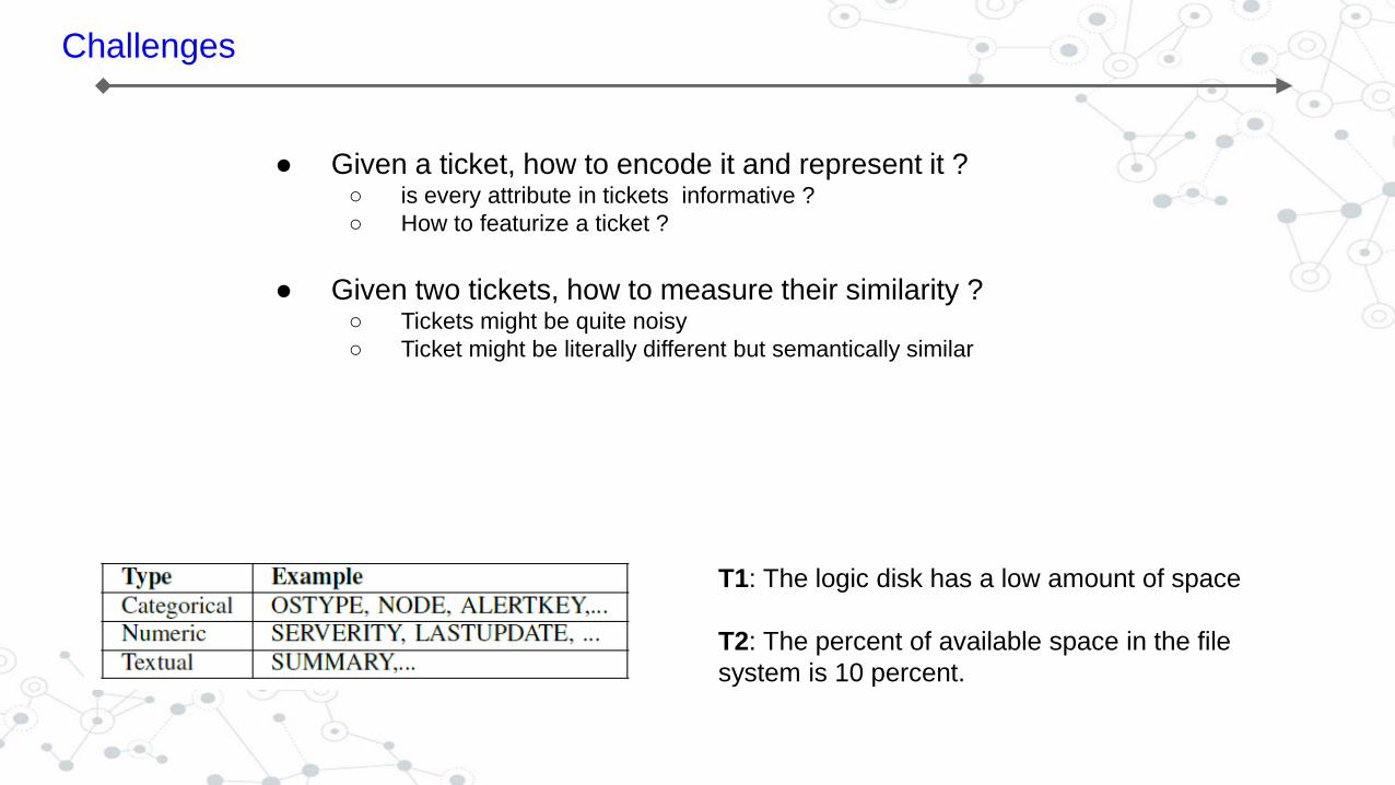
● Given a ticket, how to encode it and represent it ? ○ is every attribute in tickets informative ?
○ How to featurize a ticket ?
● Given two tickets, how to measure their similarity ? ○ Tickets might be quite noisy
○ Ticket might be literally different but semantically similar
T1: The logic disk has a low amount of space
T2: The percent of available space in the file
system is 10 percent.
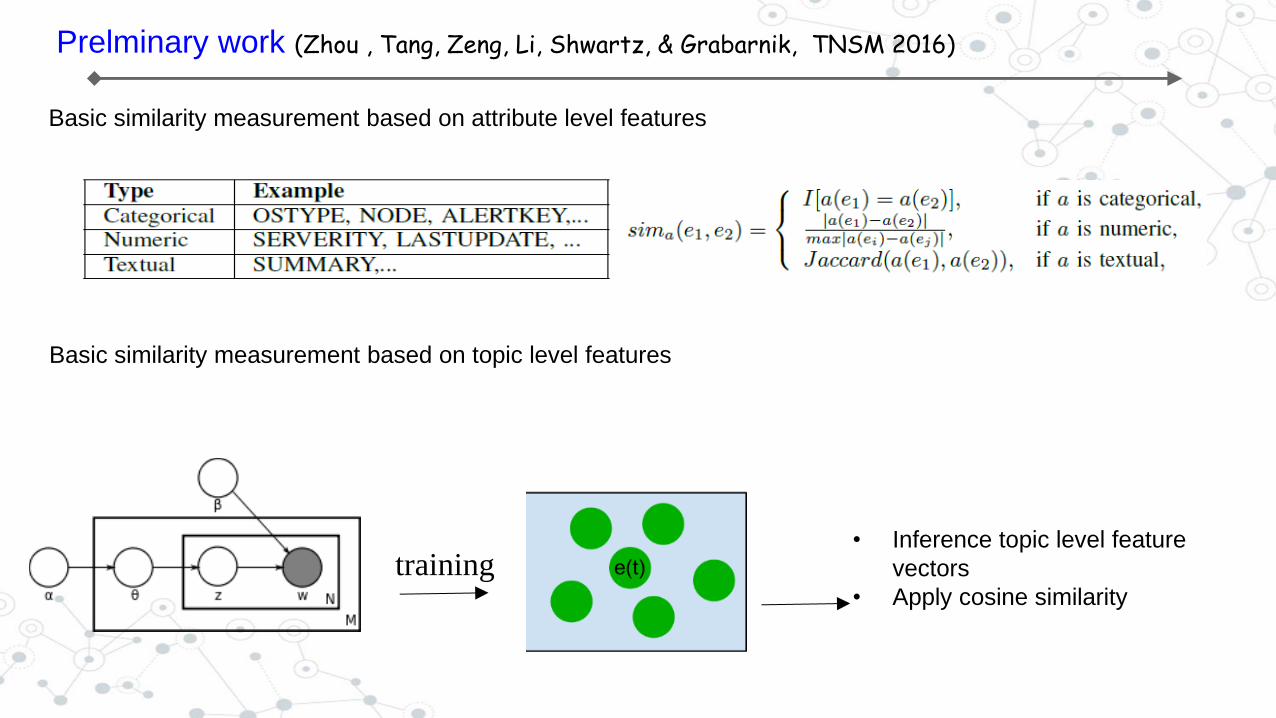
Prelminary work (Zhou , Tang, Zeng, Li, Shwartz, & Grabarnik, TNSM 2016)
Basic similarity measurement based on attribute level features
Basic similarity measurement based on topic level features
training • Inference topic level feature
vectors
• Apply cosine similarity
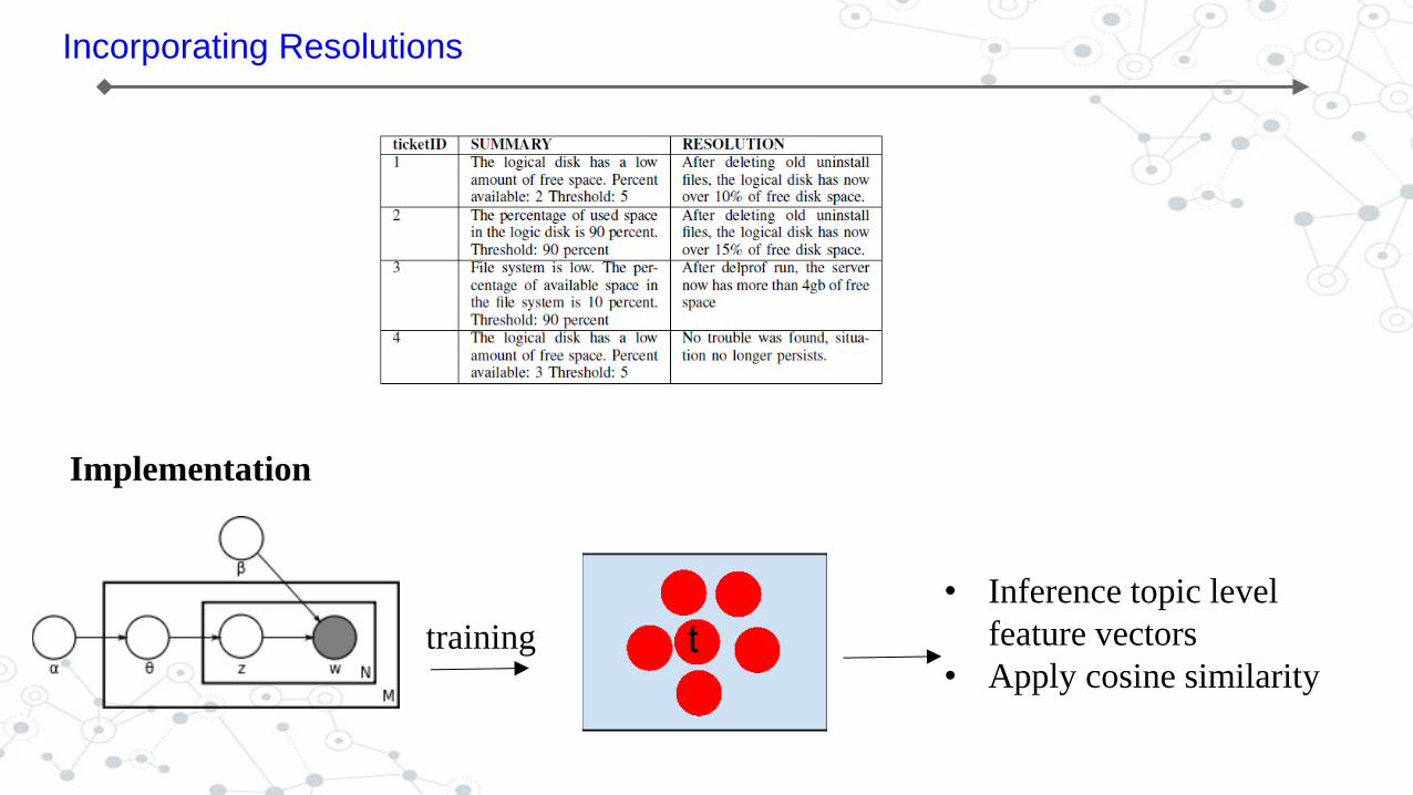
Incorporating Resolutions
Implementation
training
• Inference topic level
feature vectors
• Apply cosine similarity
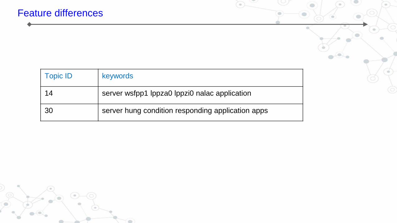
Feature differences
Topic ID keywords
14 server wsfpp1 lppza0 lppzi0 nalac application
30 server hung condition responding application apps
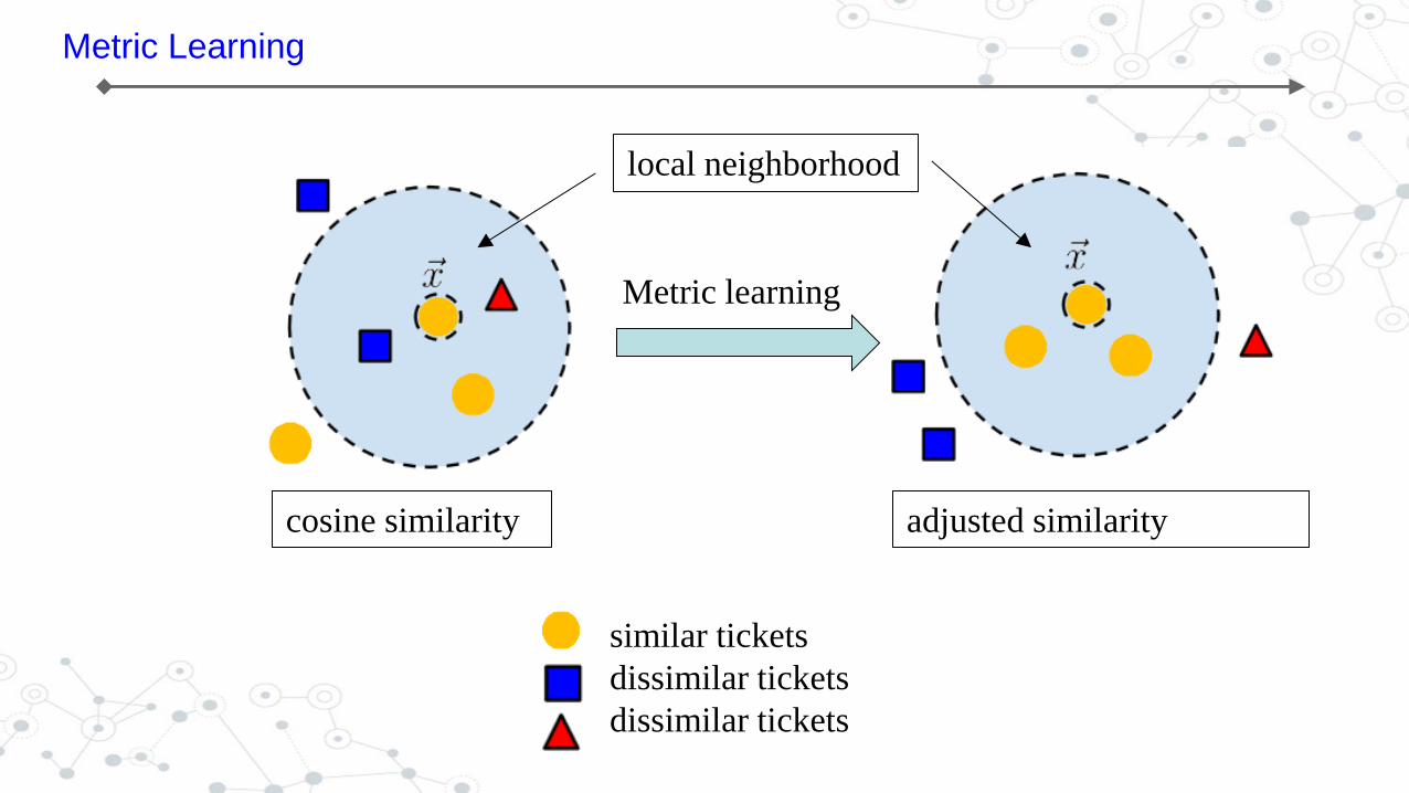
Metric Learning
local neighborhood
cosine similarity adjusted similarity
Metric learning
similar tickets
dissimilar tickets
dissimilar tickets
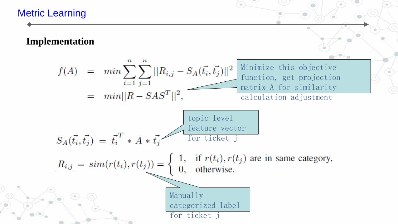
Metric Learning
Implementation
topic level feature vector for ticket j
Manually categorized label for ticket j
Minimize this objective function, get projection matrix A for similarity calculation adjustment
• Ticket Classification
• Ticket Resolution Recommendation
• Ticket Analysis (Knowledge Extraction)
Outline
Transitioning from practitioner-driven technology-assisted to technology-driven
and practitioner-assisted delivery of services
• Enterprises and service providers are increasingly challenged with improving the quality of service
delivery
• The increasing complexity of IT environments dictates the usage of intelligent automation driven by
cognitive technologies, aiming at providing higher quality and more complex services.
• Software monitoring systems are designed to actively collect and signal anomalous behavior and,
when necessary, automatically generate incident tickets.
• Solving these IT tickets is frequently a very labor-intensive process.
• Full automation of these service management processes are needed to target an ultimate goal of
maintaining the highest possible quality of IT services. Which is hard!
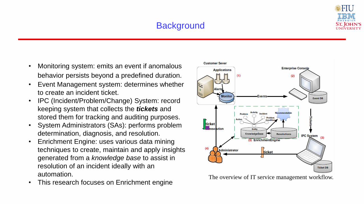
Background
• Monitoring system: emits an event if anomalous
behavior persists beyond a predefined duration.
• Event Management system: determines whether
to create an incident ticket.
• IPC (Incident/Problem/Change) System: record
keeping system that collects the tickets and
stored them for tracking and auditing purposes.
• System Administrators (SAs): performs problem
determination, diagnosis, and resolution.
• Enrichment Engine: uses various data mining
techniques to create, maintain and apply insights
generated from a knowledge base to assist in
resolution of an incident ideally with an
automation.
• This research focuses on Enrichment engine The overview of IT service management workflow.
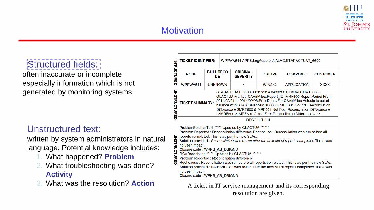
Motivation
A ticket in IT service management and its corresponding
resolution are given.
Structured fields: often inaccurate or incomplete
especially information which is not
generated by monitoring systems
Unstructured text: written by system administrators in natural
language. Potential knowledge includes:
1. What happened? Problem
2. What troubleshooting was done?
Activity
3. What was the resolution? Action
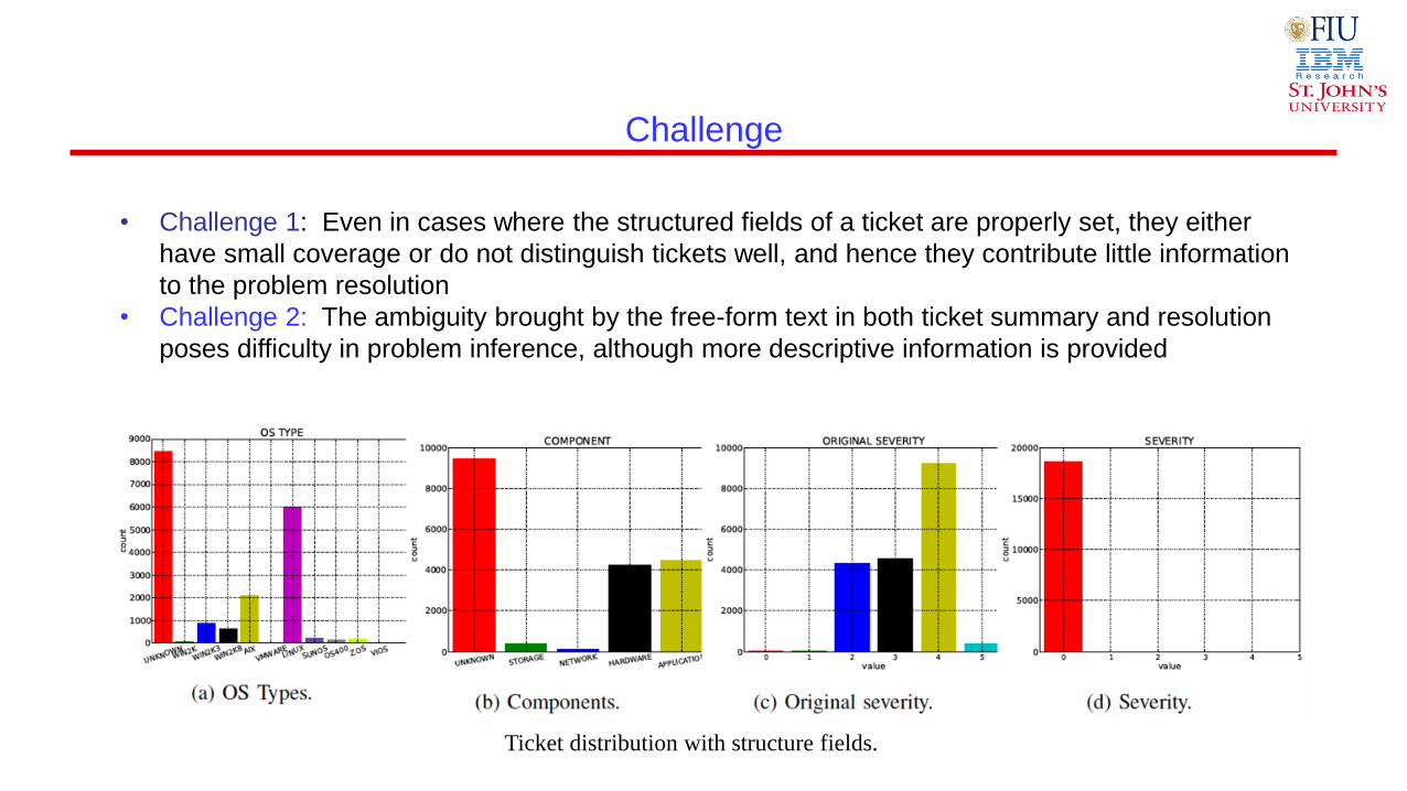
Challenge
• Challenge 1: Even in cases where the structured fields of a ticket are properly set, they either
have small coverage or do not distinguish tickets well, and hence they contribute little information
to the problem resolution
• Challenge 2: The ambiguity brought by the free-form text in both ticket summary and resolution
poses difficulty in problem inference, although more descriptive information is provided
Ticket distribution with structure fields.
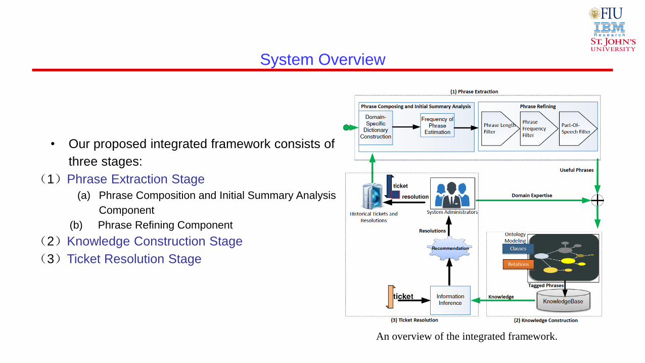
System Overview
An overview of the integrated framework.
• Our proposed integrated framework consists of
three stages:
(1)Phrase Extraction Stage
(a) Phrase Composition and Initial Summary Analysis
Component
(b) Phrase Refining Component
(2)Knowledge Construction Stage
(3)Ticket Resolution Stage
Phrase Extraction Stage
• In this stage, our framework finds important domain-specific
words and phrases (‘kernel’).
• Constructing domain-specific dictionary
• Mining the repeated words and phrases from unstructured
text field.
• Refining these repeated phrases by diverse criteria filters
(e.g., length, frequency, etc.).
Phrase Composition and Initial Summary Analysis
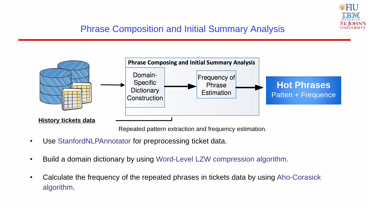
• Use StanfordNLPAnnotator for preprocessing ticket data.
• Build a domain dictionary by using Word-Level LZW compression algorithm.
• Calculate the frequency of the repeated phrases in tickets data by using Aho-Corasick
algorithm.
History tickets data
Hot Phrases Patten + Frequence
Repeated pattern extraction and frequency estimation.
Phrase Composition and Initial Summary Analysis
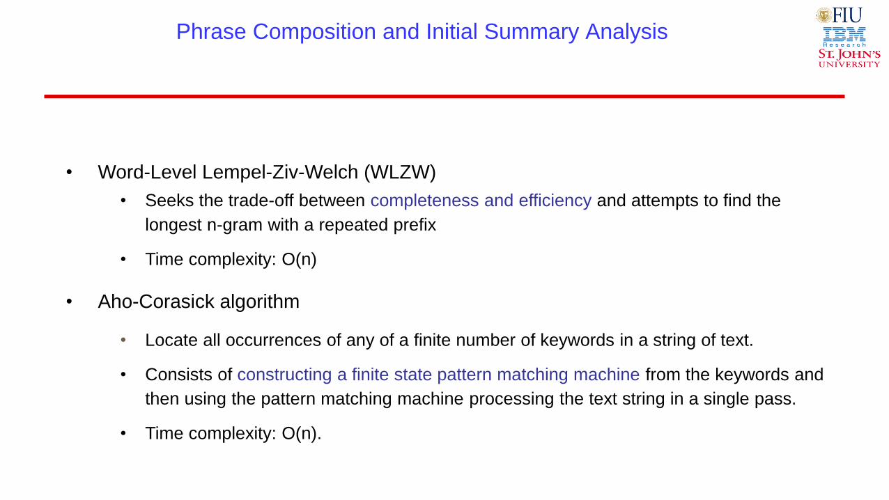
• Word-Level Lempel-Ziv-Welch (WLZW)
• Seeks the trade-off between completeness and efficiency and attempts to find the
longest n-gram with a repeated prefix
• Time complexity: O(n)
• Aho-Corasick algorithm
• Locate all occurrences of any of a finite number of keywords in a string of text.
• Consists of constructing a finite state pattern matching machine from the keywords and
then using the pattern matching machine processing the text string in a single pass.
• Time complexity: O(n).
Phrase Composition and Initial Summary Analysis
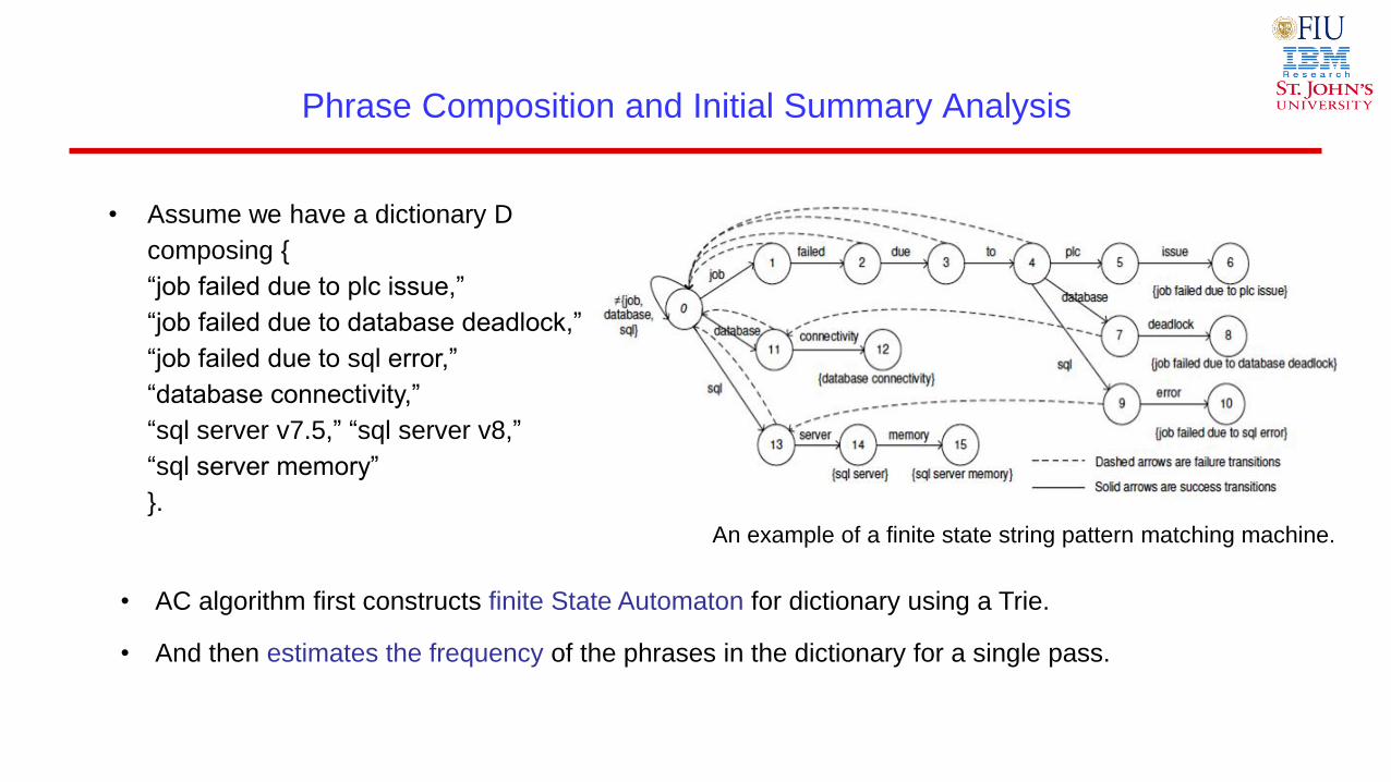
An example of a finite state string pattern matching machine.
• Assume we have a dictionary D
composing {
“job failed due to plc issue,”
“job failed due to database deadlock,”
“job failed due to sql error,”
“database connectivity,”
“sql server v7.5,” “sql server v8,”
“sql server memory”
}.
• AC algorithm first constructs finite State Automaton for dictionary using a Trie.
• And then estimates the frequency of the phrases in the dictionary for a single pass.
Phrases Refining
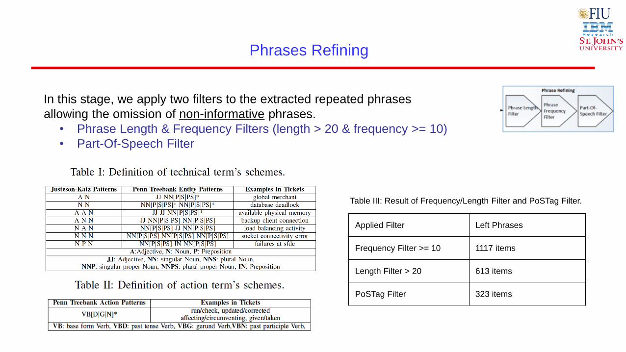
In this stage, we apply two filters to the extracted repeated phrases
allowing the omission of non-informative phrases.
• Phrase Length & Frequency Filters (length > 20 & frequency >= 10)
• Part-Of-Speech Filter
Applied Filter Left Phrases
Frequency Filter >= 10 1117 items
Length Filter > 20 613 items
PoSTag Filter 323 items
Table III: Result of Frequency/Length Filter and PoSTag Filter.
Knowledge Construction Stage
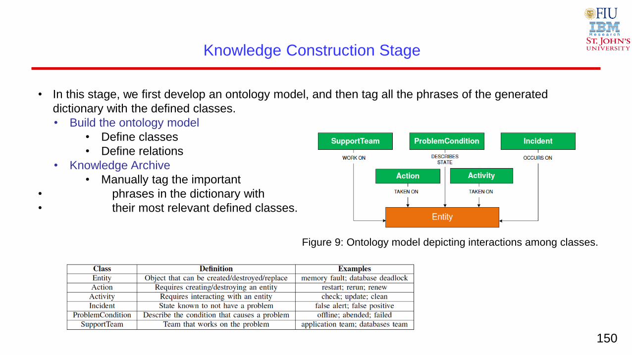
• In this stage, we first develop an ontology model, and then tag all the phrases of the generated
dictionary with the defined classes.
• Build the ontology model
• Define classes
• Define relations
• Knowledge Archive
• Manually tag the important
• phrases in the dictionary with
• their most relevant defined classes.
Figure 9: Ontology model depicting interactions among classes.
150
Knowledge Construction Stage
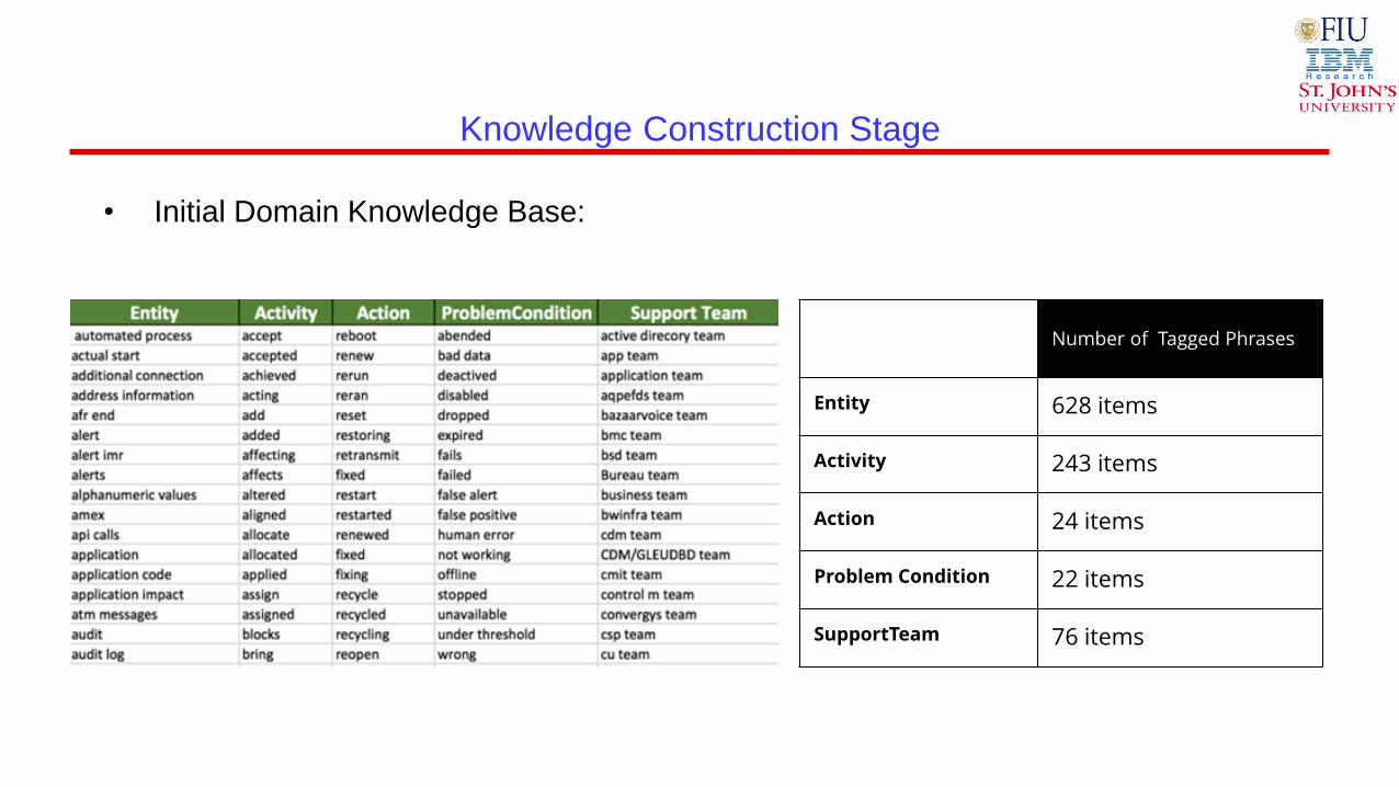
• Initial Domain Knowledge Base:
Class Number of Tagged Phrases
Entity 628 items
Activity 243 items
Action 24 items
Problem Condition 22 items
SupportTeam 76 items
Ticket Resolution Stage
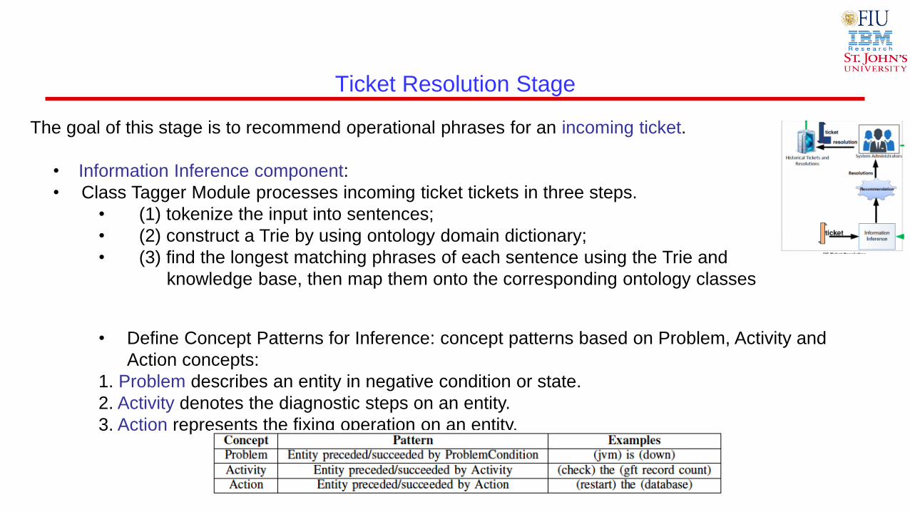
The goal of this stage is to recommend operational phrases for an incoming ticket.
• Information Inference component:
• Class Tagger Module processes incoming ticket tickets in three steps.
• (1) tokenize the input into sentences;
• (2) construct a Trie by using ontology domain dictionary;
• (3) find the longest matching phrases of each sentence using the Trie and
knowledge base, then map them onto the corresponding ontology classes
• Define Concept Patterns for Inference: concept patterns based on Problem, Activity and
Action concepts:
1. Problem describes an entity in negative condition or state.
2. Activity denotes the diagnostic steps on an entity.
3. Action represents the fixing operation on an entity.
Ticket Resolution Stage
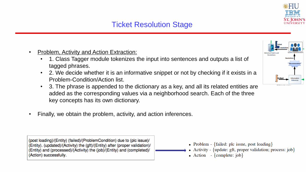
• Problem, Activity and Action Extraction:
• 1. Class Tagger module tokenizes the input into sentences and outputs a list of
tagged phrases.
• 2. We decide whether it is an informative snippet or not by checking if it exists in a
Problem-Condition/Action list.
• 3. The phrase is appended to the dictionary as a key, and all its related entities are
added as the corresponding values via a neighborhood search. Each of the three
key concepts has its own dictionary.
• Finally, we obtain the problem, activity, and action inferences.
Ticket Resolution Stage
• The goal of this stage is to recommend operational phrases for an incoming ticket. • Ontology-based Resolution Recommendation component
• Previous study, the KNN-based algorithm will be used to recommend the historical
tickets’ resolution to the incoming ticket which have the top summary similarity scores.
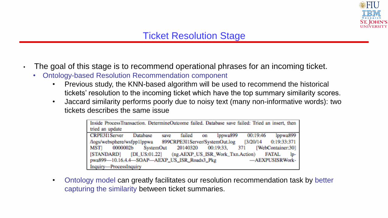
• Jaccard similarity performs poorly due to noisy text (many non-informative words): two
tickets describes the same issue
• Ontology model can greatly facilitates our resolution recommendation task by better
capturing the similarity between ticket summaries.
Experiment
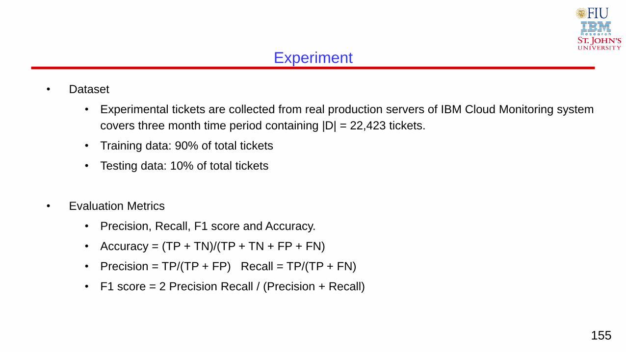
• Dataset
• Experimental tickets are collected from real production servers of IBM Cloud Monitoring system
covers three month time period containing |D| = 22,423 tickets.
• Training data: 90% of total tickets
• Testing data: 10% of total tickets
• Evaluation Metrics
• Precision, Recall, F1 score and Accuracy.
• Accuracy = (TP + TN)/(TP + TN + FP + FN)
• Precision = TP/(TP + FP) Recall = TP/(TP + FN)
• F1 score = 2 Precision Recall / (Precision + Recall)
155
Experiment
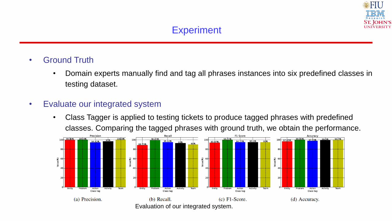
• Ground Truth
• Domain experts manually find and tag all phrases instances into six predefined classes in
testing dataset.
• Evaluate our integrated system
• Class Tagger is applied to testing tickets to produce tagged phrases with predefined
classes. Comparing the tagged phrases with ground truth, we obtain the performance.
Evaluation of our integrated system.
Experiment
• Evaluate Information Inference
• Usability: we evaluate the average accuracy to be 95.5%, 92.3%, and 86.2% for
Problem, Activity, and Action respectively.
• Readability: we measure the time cost. Domain expert can be quicker to identity
the Problem, Activity and Action which output from the Information Inference
component from 50 randomly selected tickets.
Introduction and Overview
Contents
1
Event Generation and System Monitoring
2
Pattern Discovery and Summarization
3
Conclusions 5
Mining with Events and Tickets 4
159
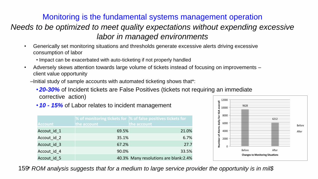
Monitoring is the fundamental systems management operation Needs to be optimized to meet quality expectations without expending excessive
labor in managed environments • Generically set monitoring situations and thresholds generate excessive alerts driving excessive
consumption of labor
• Impact can be exacerbated with auto-ticketing if not properly handled
• Adversely skews attention towards large volume of tickets instead of focusing on improvements –
client value opportunity
–Initial study of sample accounts with automated ticketing shows that*:
• 20-30% of Incident tickets are False Positives (tickets not requiring an immediate
corrective action)
• 10 - 15% of Labor relates to incident management
15
9
Account % of monitoring tickets for the account
% of false positives tickets for the account
Accout_id_1 69.5% 21.0%
Accout_id_2 35.1% 6.7%
Accout_id_3 67.2% 27.7
Accout_id_4 90.0% 33.5%
Accout_id_5 40.3% Many resolutions are blank:2.4%
* ROM analysis suggests that for a medium to large service provider the opportunity is in mil$
9628
6212
0
2000
4000
6000
8000
10000
12000
Before A er
NumberofAlertsdailyforIGAoverall
ChangestoMonitoringSitua ons
Before
A er
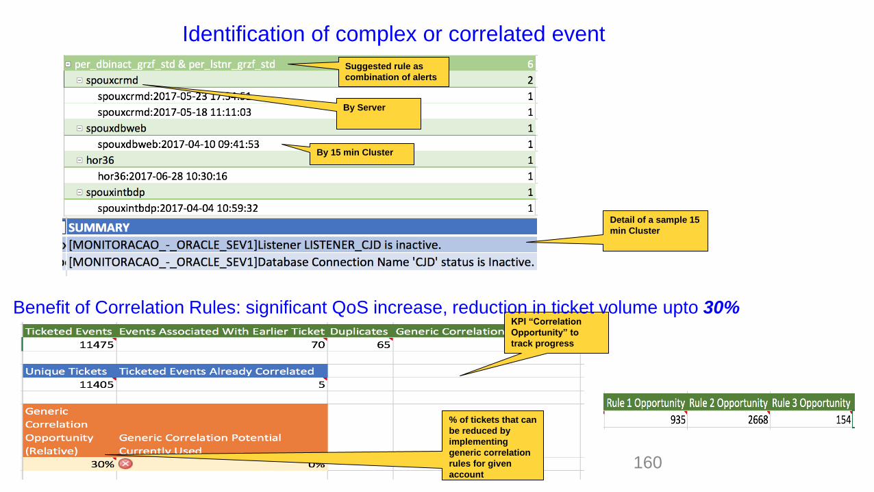
Identification of complex or correlated event
160
Suggested rule as
combination of alerts
By Server
By 15 min Cluster
Detail of a sample 15
min Cluster
KPI “Correlation
Opportunity” to
track progress
% of tickets that can
be reduced by
implementing
generic correlation
rules for given
account
Benefit of Correlation Rules: significant QoS increase, reduction in ticket volume upto 30%
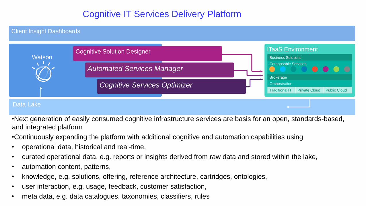
Cognitive Solution Designer
Cognitive Services Optimizer
Automated Services Manager
Client Insight Dashboards
Data Lake
Watson
ITaaS Environment
Business Solutions
Composable Services
Brokerage
Orchestration
Traditional IT Private Cloud Public Cloud
Cognitive IT Services Delivery Platform
•Next generation of easily consumed cognitive infrastructure services are basis for an open, standards-based,
and integrated platform
•Continuously expanding the platform with additional cognitive and automation capabilities using
• operational data, historical and real-time,
• curated operational data, e.g. reports or insights derived from raw data and stored within the lake,
• automation content, patterns,
• knowledge, e.g. solutions, offering, reference architecture, cartridges, ontologies,
• user interaction, e.g. usage, feedback, customer satisfaction,
• meta data, e.g. data catalogues, taxonomies, classifiers, rules
What Log/Event Analysis Can Do I
• Proactively monitors system resources to detect potential problems and automatically
respond to events.
– By identifying issues early, it enables rapid fixes before users notice any
difference in performance.
• Provides dynamic thresholding and performance analytics to improve incident
avoidance.
– This ‘early warning’ system allows you to start working on an incident before it
impacts users, business applications or business services.
• Improves availability and mean-to-time recovery with quick incident visualization and
historical look for fast incident research.
– You can identify and take action on a performance or service interruption in
minutes rather than hours.
What Log/Event Analysis Can Do II
• Collects data you can use to drive timely performance and capacity planning activities
to avoid outages from resource over-utilization.
– The software monitors, alerts and reports on future capacity bottlenecks.
• Facilitates system monitoring with a common, flexible and intuitive browser interface
and customizable workspaces.
– Can include an easy-to-use data warehouse and advanced reporting capabilities..
Looking Forward
• Real-time requirements
• Failure prediction
• Incorporation domain knowledge with mining results
• Integration of different types of information
• From systems to networks and devices
• Limited labeled data
• Interpretation and Transparency
Acknowledgements
• Funding
– National Science Foundation
– IBM Research
– Simons Foundation
• Ph.D. Students working on Log/Event/Ticket mining
– Dr. Wei Peng (Google)
– Dr. Yexi Jiang (Facebook)
– Dr. Liang Tang (LinkedIn)
– Dr. Chao Shen (Amazon)
– Dr. Chunqiu Zeng (Google)
– Wubai Zhou (FIU)
– Qing Wang (FIU)
Thank you!
Email: [email protected]
All the slides and references can be found at
http://www.cs.fiu.edu/~taoli/event-mining