entropy balancing for causal effects: a multivariate ...jhain/paper/pa2012.pdfentropy balancing for...
TRANSCRIPT
Advance Access publication October 16, 2011 Political Analysis(2012) 20:25−46doi:10.1093/pan/mpr025
Entr opy Balancing for Causal Effects: A MultivariateReweighting Method to Produce Balanced Samples
in Observational Studies
Jens HainmuellerDepartment of Political Science, Massachusetts Institute of Technology,
77 Massachusetts Avenue, Cambridge, MA 02139e-mail: [email protected]
Editedby R. Michael Alvarez
This paper proposes entropy balancing, a data preprocessing method to achieve covariate balance inobservational studies with binary treatments. Entropy balancing relies on a maximum entropy reweightingscheme that calibrates unit weights so that the reweighted treatment and control group satisfy a potentiallylarge set of prespecified balance conditions that incorporate information about known sample moments.Entropy balancing thereby exactly adjusts inequalities in representation with respect to the first, second,and possibly higher moments of the covariate distributions. These balance improvements can reducemodel dependence for the subsequent estimation of treatment effects. The method assures that balanceimproves on all covariate moments included in the reweighting. It also obviates the need for continualbalance checking and iterative searching over propensity score models that may stochastically balancethe covariate moments. We demonstrate the use of entropy balancing with Monte Carlo simulations andempirical applications.
1 Intr oduction
Matching and propensity score methods are nowadays often used in observational studies in politicalscience and other disciplines to preprocess the data prior to the estimation of binary treatment effectsunder the assumption of selection on observables (Ho et al. 2007; Sekhon 2009). The preprocessing stepinvolves reweighting or simply discarding units to improve the covariate balance between the treatmentand control group such that the treatment variable becomes closer to being independent of the backgroundcharacteristics. This reduces model dependence for the subsequent estimation of treatment effects withregression or other standard estimators in the preprocessed data (Abadie and Imbens 2007; Ho et al.2007).
Although preprocessing methods are gaining ground in applied work, there exists no scholarly con-sensus in the methodological literature about how the preprocessing step is best conducted. One impor-tant concern is that many commonly used preprocessing approaches do not directly focus on the goal ofproducing covariate balance. In the most widely used practice, researchers “manually” iterate betweenpropensity score modeling, matching, and balance checking until they attain a satisfactory balancing solu-tion. The hope is that an accurately estimated propensity score will stochastically balance the covariates,but this requires finding the correct model specification and often fairly large samples. As a result of this
Author’s note:The author is also affiliated with Harvard’s Institute for Quantitative Social Science (IQSS). I thank Alberto Abadie,Alexis Diamond, Andy Eggers, Adam Glynn, Don Green, Justin Grimmer, Dominik Hangartner, Dan Hopkins, Kosuke Imai, GuidoImbens, Gary King, Gabe Lenz, Jasjeet Sekhon, and Yiqing Xu for very helpful comments. I would especially like to thank AlanZaslavsky, who inspired this project. I would also like to thank the editor R. Michael Alvarez and our three anonymous reviewersfor their excellent suggestions. The usual disclaimer applies.
Companion software (for Stata and R) that implements the methods proposed in this paper is provided on the author’s webpage.Replication materials are available in the Political Analysis Dataverse athttp://dvn.iq.harvard.edu/dvn/dv/pan. Supplementarymaterials for this article are available on thePolitical AnalysisWeb site.
c© TheAuthor 2011. Published by Oxford University Press on behalf of the Society for Political Methodology.All rights reserved. For Permissions, please email: [email protected]
25
at Stanford University on D
ecember 4, 2015
http://pan.oxfordjournals.org/D
ownloaded from

26 Jens Hainmueller
intricatesearch process, low balance levels prevail in many studies and the user experience can be tedious.Even worse, matching may counteract bias reduction for the subsequent treatment effect estimation whenimproving balance on some covariates decreases balance on other covariates (seeDiamond and Sekhon2006,Ho et al. 2007, andIacus, King, and Porro 2009for similar critiques).
In this study, we propose entropy balancing as a preprocessing technique for researchers to achievecovariate balance in observational studies with a binary treatment. In contrast to most other preprocessingmethods, entropy balancing involves a reweighting scheme that directly incorporates covariate balanceinto the weight function that is applied to the sample units. The researcher begins by imposing a poten-tially large set of balance constraints, which imply that the covariate distributions of the treatment andcontrol group in the preprocessed data match exactly on all prespecified moments. After the researcherhas prespecified her desired level of covariate balance, entropy balancing searches for the set of weightsthat satisfies the balance constraints but remains as close as possible (in an entropy sense) to a set ofuniform base weights to retain information. This recalibration of the unit weights effectively adjusts forsystematic and random inequalities in representation.
This procedure has several attractive features. Most importantly, entropy balancing allows the researcherto obtain a high degree of covariate balance by imposing a potentially large set of balance constraints thatinvolve the first, second, and possibly higher moments of the covariate distributions as well as interac-tions. Entropy balancing always (at least weakly) improves upon the balance that can be obtained byconventional preprocessing adjustments with respect to the specified balance constraints. This is becausethe reweighting scheme directly incorporates the researcher’s knowledge about the known sample mo-ments and balances them exactly in finite samples (analogous to similar reweighting procedures in surveyresearch that improve inferences about unknown population features by adjusting the sample to someknown population features). This obviates the need for balance checking in the conventional sense, atleast for the characteristics that are included in the specified balance constraints.
A second advantage of entropy balancing is that it retains valuable information in the preprocesseddata by allowing the unit weights to vary smoothly across units. In contrast to other preprocessing meth-ods such as nearest neighbor matching where units are either discarded or matched (weights of zero orone)1 , the reweighting scheme in entropy balancing is more flexible: It reweights units appropriately toachieve balance, but at the same time keeps the weights as close as possible to the base weights to pre-vent loss of information and thereby retains efficiency for the subsequent analysis. In this regard, entropybalancing provides a generalization of the propensity score weighting approach (Hirano, Imbens, andRidder 2003) where the researcher first estimates the propensity score weights with a logistic regressionand then computes balance checks to see if the estimated weights equalize the covariate distributions. Inpractice, such estimated propensity score weights can fail to balance the covariate moments in finite sam-ples. Entropy balancing in contrast directly adjusts the weights to the known sample moments and therebyobviates the need for continual balance checking and iterative searching over propensity score models thatmay stochastically balance the prespecified covariates.
A third advantage of entropy balancing is that the approach is fairly versatile. The weights that resultfrom entropy balancing can be passed to almost any standard estimator for the subsequent estimation oftreatment effects. This may include a simple (weighted) difference in means, a weighted least squares re-gression of the outcome on the treatment variable and possibly additional covariates that are not includedas part of the reweighting, or whatever other standard statistical model the researcher would have ap-plied in the absence of any preprocessing. Since entropy balancing orthogonalizes the treatment indicatorwith respect to the covariates that are included in the balance constraints, the resulting estimates in thepreprocessed data can exhibit lower model dependency compared to estimates from the unadjusted data.
Lastly, entropy balancing is also computationally attractive since the optimization problem to find theunit weights is well behaved and globally convex; the algorithm attains the weighting solution withinseconds even for moderately large data sets that may be encountered in political science applications(assuming that the balance constraints are feasible).
We show three Monte Carlo simulations that demonstrate the desirable finite sample properties of en-tropy balancing in several benchmark settings where the method improves in root mean squared error
1In practice, the weights may sometimes differ from zero or one in the case of ties or for controls units that are matched severaltimes when matching with replacement.
at Stanford University on D
ecember 4, 2015
http://pan.oxfordjournals.org/D
ownloaded from

Entropy Balancing for Causal Effects 27
(MSE) upon a variety of widely used preprocessing adjustments (including Mahalanobis distance match-ing, genetic matching, and matching or weighting on a logistic propensity score). We also illustrate the useof entropy balancing in two empirical settings including a validation exercise in theLaLonde(1986) dataset and a reanalysis of the data used byLadd and Lenz(2009) to examine the effect of newspaper endorse-ments on vote choice in the 1997 British general election. Two additional applications that consider theimpact of media bias on voting (DellaVigna and Kaplan 2007) and the financial returns to political office(Eggers and Hainmueller 2009) are provided in a web appendix.2 Entropy balancing yields high levels ofcovariate balance (as measured by standard metrics) in all four data sets and reduces model dependencyfor the subsequent estimation of the treatment effects.
Although entropy balancing provides a reweighting scheme for the context of causal inference in ob-servational studies with a binary treatment (where the goal is to equate the covariate distributions acrossthe treatment and the control group), important links exist between the reweighting scheme employedin entropy balancing and various strands of literatures in econometrics and statistics. In particular, themethod heavily borrows from the survey literature that contains several reweighting schemes which areused to adjust sampling weights so that sample totals match population totals known from auxiliary data(seeSarndal and Lundstrom 2006for a recent review and earlier work byDeming and Stephan 1940, Ire-land and Kullback 1968, Oh and Scheuren 1978, andZaslavsky 1988who proposed a similar log-linearreweighting scheme to adjust for undercount in census data). More broadly, similar reweighting schemesare also widely used in the literature on methods of moments estimation, empirical likelihood, exponen-tial tilting, and missing data (Hansen 1982;Qin and Lawless 1994;Kitamura and Stutzer 1997; Imbens1997; Imbens, Spady, and Johnson 1998;Hellerstein and Imbens 1999;Owen 2001;Schennach 2007;Qin, Zhang, and Leung 2009;Graham, Pinto, and Egel 2010).
2 Observational Studies with Binary Treatments
2.1 Framework
We consider a random sample ofn = n1 +n0 unitsdrawn from a population of sizeN = N1 + N0, wheren 6 N andN1 andN0 referto the size of the target population of treated units and the source populationof control units, respectively. Each uniti is exposed to a binary treatmentDi ∈ {1,0}; Di = 1 if unit ireceived the active treatment andDi = 0 if unit i received the control treatment. In the sample, we haven1 treatedunits andn0 controlunits. LetX be a matrix ofJ exogenous pretreatment characteristics; entryXi j refersto the value of thej th characteristic for uniti so thatXi = [Xi 1, Xi 2, . . . , Xi J ] is the rowvector of characteristics for uniti andX j is the column vector that captures thej th characteristic acrossunits accordingly. LetfX|D=1 and fX|D=0 denotethe densities of these covariates in the treatment andcontrol population, respectively. Finally, letYi (Di ) denotethe pair of potential outcomes that individuali attains if it is exposed to the active treatment or the control treatment. Observed outcomes for eachindividual are realized asYi = Yi (1) Di + (1− Di )Yi (0) sothat we never observe both potential outcomessimultaneously but the triple (Di , Yi , Xi ).
Thetreatment effect for each unit is defined asτi = Yi (1) − Yi (0). Many causal quantities of interestare defined as functions ofτi for different subsets of units.3 Most common are the sample (SATE) andpopulation (PATE) average treatment effects given by SATE= n−1∑n
i τi andPATE = N−1∑Ni τi and
the sample (SATT) and population (PATT) average treatment effect on the treated given by SATT=n−1
1∑n
{i |D=1} τi andPATT = N−11∑N
{i |D=1} τi . Notice thatE[SATE] = PATE = E[Y(1) − Y(0)] andsimilarlyE[SATT] = PATT = E[Y(1)− Y(0)|D = 1] since we consider random samples. Following thepreprocessing literature, we focus on the PATT as our quantity of interest. The entropy balancing methodsdescribed below are also applicable to estimate the PATE and other commonly used quantities of interestanalogously.4
The PATT is given byτ = E[Y(1)|D = 1] − E[Y(0)|D = 1]. The first expectation is easily es-timable from the treatment group data. The second expectation,E[Y(0)|D = 1], is counterfactual and
2Thisweb appendix is available on the authors webpage athttp://www.mit.edu/ jhainm/research.htm.3Notethat some other causal quantities of interest are not defined in this way (e.g., causal mediation or necessary causation).4For example, the treatment group can be reweighted to match the control group. An important caveat is that it may be more difficultto estimate the PATE or SATE due to limited overlap in the covariate distributions.
at Stanford University on D
ecember 4, 2015
http://pan.oxfordjournals.org/D
ownloaded from

28 Jens Hainmueller
thusunobserved even in the target population. The only information available aboutY(0) is in the sam-ple from the source population not exposed to the treatment (the control group). In experimental studies,where treatment assignment is forced to be independent of the potential outcomes,Y(1),Y(0) ⊥ D, wecan simply useE[Y(0)|D = 0] as our estimate ofE[Y(0)|D = 1]. In observational studies, however,selection into treatment usually renders the latter two quantities unequal. The conventional solution to thisproblem is to assume ignorable treatment assignment and overlap (Rosenbaum and Rubin 1983), whichimplies thatY(0) ⊥ D|X and that Pr(D = 1|X = x) < 1 for all x in the support offX|D=1. Therefore,conditional on all confounding covariatesX, the potential outcomes are stochastically independent ofDand the PATT is identified as
τ = E[Y|D = 1] −∫E[Y|X = x, D = 0] fX|D=1(x)dx,
wherethe integral is taken over the support ofX in the source population. Notice that the last term inthis expression is equal to the covariate adjusted mean, that is, the estimated mean ofY in the sourcepopulation if its covariates were distributed as in the target population (Frolich 2007).
To see why covariate balance is key for the estimation of the PATT, notice that the potential outcomesfor the treated units can be written asYi (Di ) = l (Xi ), wherel () is an unknown function. For simplicity,suppose that the treatment effect is estimated by the difference in means. The treatment effect can then bedecomposed into the estimated treatment effect and the average estimation error:
PATT = PATT + N−11
∑
{i |D=1}
(l0(X{i |D=0}) − l0(X{i |D=1})),
wherel0(X{i |D=0}) − l0(X{i |D=1}) = Yi (0) − Yi (0) is the unit level treatment error (seeIacus, King, andPorro 2009). The estimation error has two components: (1) the unknown functionl (), which determinesthe importance of the variables, and (2) the imbalance, which is defined as the difference between theempirical covariate distributions of the treatmentfX|D=1 andthe control groupfX|D=0.
Datapreprocessing procedures such as matching and related approaches involve reweighting or simplydiscarding units to reduce the imbalance in the covariate distributions to decrease the error and model de-pendency for the subsequent estimation of the treatment effect. AsHo et al.(2007, 209) put it, “the goal ofmatching is to achieve the best balance for a large number of observations, using any method of matchingthat is a function ofX, so long as we do not consultY.”5 A variety of such preprocessing procedures havebeen proposed (Imbens 2004;Rubin 2006;Ho et al. 2007; Sekhon 2009). IfX is low dimensional, theunits can simply be matched exactly on the covariates. However, selection on observables is often onlyplausible after conditioning on many confounders and ifX is fairly high dimensional then the curse of di-mensionality can render exact matching infeasible. However, as shown byRosenbaum and Rubin(1983),the preprocessing problem may be reduced to a single dimension given that the counterfactual mean canalso be identified as
E[Y(0)|D = 1] =∫E[Y|p(X) = ρ, D = 0] f p|D=1(ρ)dρ
where f p|D=1 is the distribution of the propensity scorep(x) = Pr(D = 1|X = x) in the target pop-ulation. This follows from their result that under selection on observablesY(0) ⊥ D|X is equal to
5Noticethat there is some debate about how to assess covariate balance in practice. Theoretically, we would like the two empiricaldistributions to be equal so that the density in the preprocessed control groupf ∗
X|D=0 mirrorsthe density in the treatment groupfX|D=1. Comparing the joint empirical distributions of all covariatesX is difficult when X is high dimensional and thereforelower dimensional balance metrics are commonly used (but seeIacus, King, and Porro 2009who propose a multidimensionalmetric). Opinions differ on what metric is most appropriate. The most commonly used metric is the standardized difference inmeans (Rosenbaum and Rubin 1983) and t-tests for differences in means.Diamond and Sekhon(2006) argue that pairedt-testand bootstrapped Kolmogorov–Smirnov (KS) tests should be used instead and that commonly usedp value cutoffs such as .1 or.05 are too lenient to obtain reliable causal inferences.Rubin (2006) also considers variance ratios and tests for residuals thatare orthogonalized to the propensity score.Imai, King, and Stuart(2008) criticize the use oft-tests and stopping rules and arguethat all balance measures should be maximized without limit. They advocate QQ plot summary statistics as better alternativesthant-tests or KS tests.Sekhon(2006) comes to the opposite conclusion.Hansen and Bowers(2008) advocate the use of Fisher’srandomization inference for balance checking.
at Stanford University on D
ecember 4, 2015
http://pan.oxfordjournals.org/D
ownloaded from
Entropy Balancing for Causal Effects 29
Y(0) ⊥ D|p(x) andthis implies that balance on all covariates can be achieved by matching or weightingon the propensity score alone.
The procedure of particular interest here involves weighting on the propensity score as suggested byHirano and Imbens(2001) andHirano, Imbens, and Ridder(2003). In this method, the researcher firstestimates a propensity score (usually by a logit or probit regression of the treatment indicator on thecovariates) and then the units are weighted by the inverse of this estimated score for the subsequentanalysis. For example, the counterfactual mean in the preprocessed data may be estimated using
E[Y(0)|D = 1] =
∑{i |D=0} Yi di∑
{i |D=0} di,
whereevery control unit receives a weight given bydi = p(xi )1−p(xi )
. If the assignment probabilities are cor-rectly estimated by the propensity score model, then the control observations will form a balanced samplewith the treated observations in the reweighted data.6 Theidea is similar to the classic Horvitz–Thompsonadjustment used in the survey literature where units are weighted by the inverse of the inclusion probabil-ities that result from the sampling design (Horvitz and Thompson 1952). This similarity between surveysampling weights and propensity score weights provides the entry point for the reweighting methodsproposed below.
2.2 Achieving Balance with Matching and Propensity Score Methods
In principle, propensity score weighting has some attractive theoretical features compared to other adjust-ment techniques such as pair matching or propensity score matching.Hirano, Imbens, and Ridder(2003)show that weighting on the estimated propensity score achieves the semiparametric efficiency bound forthe estimation of average causal effects as derived inHahn(1998). This result requires sufficiently largesamples and a propensity score that is sufficiently flexibly estimated to approximate the true propensityscore.
However, in practice, this procedure suffers from the same drawbacks that plague all propensity scoremethods: the true propensity score is valuable because it is a “balancing score” that stochastically equal-izes the distributions of all covariates between the two groups, but the true score is usually unknown andoften difficult to estimate accurately enough to actually produce the desired covariate balance.7 Severalstudies have demonstrated that misspecified propensity scores can lead to substantial bias for the subse-quent estimation of treatment effects (Drake 1993;Smith and Todd 2001; Diamond and Sekhon 2006)because misspecified propensity scores can fail to balance the covariates distributions.
When estimating propensity scores in practice it is often difficult to jointly balance all covariates, es-pecially in high-dimensional data with possibly complex assignment mechanisms. Applied researchersalmost always rely on simple logit or probit models to estimate the propensity score and try to avoidmisspecification by “manually” iterating between matching or weighting, propensity score modeling, andbalance checking until a satisfactory balancing solution is reached. In other words, the resulting balanceprovides the appropriate yardstick to assess the accuracy of a propensity score model. Some researchershave criticized this cyclical process as the “propensity score tautology” (Imai, King, and Stuart 2008).The iterative process of tweaking the propensity score model and balance checking can be tedious andfrequently results in low balance levels. Even worse, asDiamond and Sekhon(2006, 8) observe, a “sig-nificant shortcoming of common matching methods such as Mahalanobis distance and propensity scorematching is that they may (and in practice, frequently do) make balance worse across measured potentialconfounders.” Unless the distributions of the covariates are ellipsoidally symmetric or are mixtures of
6Formally propensity score reweighting exploits the following equalities:E[
DYp(x)
]= E
[DY(1)p(x)
]= E
[E[
DY(1)p(x) |X
]]=
E[
p(x)Y(1)p(x)
]= E[Y(1)] which uses the ignorability assumption in the second to last equality (Hirano and Imbens 2001; Hi-
rano, Imbens, and Ridder 2003).7Hirano, Imbens, and Ridder(2003) derive their result for a case where the propensity score is estimated using a nonparametricsieve estimator that approximates the true propensity score by a power series in all variables. Asymptotically, this series willconverge to the true propensity score function if the powers increase with the sample size, but no results exist about the finitesample properties of this estimator. By the authors’ own admission, this approach is computationally not very attractive.
at Stanford University on D
ecember 4, 2015
http://pan.oxfordjournals.org/D
ownloaded from

30 Jens Hainmueller
proportionalellipsoidally symmetric distributions, there is no guarantee that the matching techniques willbe equally percent bias reducing (EPBR). Therefore, the bias of some linear functions ofX may be in-creased, whereas all univariate covariate means are closer after the preprocessing.8 Also notice that evenwith a good propensity score model, imbalances often remain because stochastic balancing occurs onlyasymptotically. Chance imbalances may remain in finite samples and in these cases one may still improvethe balance by enforcing balance constraints on the specified moments.
One way to improve the search for a better balancing score is to replace the logistic regression witha better estimation techniques for the assignment mechanism such as boosted regression (McCaffrey,Ridgeway, and Morral 2004) or kernel regression (Frolich 2007). Entropy balancing takes a differentapproach and directly focuses on covariate balance.
3 Entr opy Balancing
Entropy balancing is a preprocessing procedure that allows researchers to create balanced samples forthe subsequent estimation of treatment effects. The preprocessing consists of a reweighting scheme thatassigns a scalar weight to each sample unit such that the reweighted groups satisfy a set of balance con-straints that are imposed on the sample moments of the covariate distributions. The balance constraintsensure that the reweighted groups match exactly on the specified moments. The weights that result fromentropy balancing can be passed to any standard model that the researcher may want to use to model theoutcomes in the reweighted data—the subsequent effect analysis proceeds just like with survey samplingweights or weights that are estimated from a logistic propensity score covariate model. The preprocessingstep can reduce the model dependence for the subsequent analysis since entropy balancing orthogonalizesthe treatment indicator with respect to the covariate moments that are included in the reweighting.
3.1 Entropy Balancing Scheme
For convenience, we motivate entropy balancing for the simplest scenario where the researcher’s goal is toreweight the control group to match the moments of the treatment group in order to subsequently estimatethe PATTτ = E[Y(1)|D = 1] − E[Y(0)|D = 1] using the difference in mean outcomes between thetreatment group and the reweighted control group. In this case, the counterfactual mean may be estimatedby
E[Y(0)|D = 1] =
∑{i |D=0} Yi wi∑
{i |D=0} wi, (1)
wherewi is a weight chosen for each control unit. The weights are chosen by the following reweightingscheme:
minwi
H(w) =∑
{i |D=0}
h(wi ) (2)
subjectto balance and normalizing constraints
∑
{i |D=0}
wi cr i (Xi ) = mr with r ∈ 1, . . . , R and (3)
∑
{i |D=0}
wi = 1 and (4)
wi > 0 for all i such that D = 0, (5)
whereh(∙) is a distance metric andcr i (Xi ) = mr describesa set ofR balance constraints imposed on thecovariate moments of the reweighted control group as discussed below.
8Ellipsoidalsymmetry fails ifX includes binary, categorical, and or skewed continuous variables.
at Stanford University on D
ecember 4, 2015
http://pan.oxfordjournals.org/D
ownloaded from
Entropy Balancing for Causal Effects 31
The reweighting scheme consists of three features. First, the loss functionh(∙) is a distance metricchosen from the general class of empirical minimum discrepancy estimators defined by the Cressie–Read (CR) divergence (Read and Cressie 1988). We prefer to use the directedKullback (1959) entropydivergence defined byh(wi ) = wi l og(wi /qi ) with estimated weightwi andbase weightqi .9 The lossfunction measures the distance between the distribution of estimated control weights defined by the vectorW = [w i , . . . , wn0]′ andthe distribution of the base weights specified by the vectorQ = [qi , . . . , qn0]′
with qi > 0 for all i such thatD = 0 and∑
{i |D=0} qi = 1. Notice that the loss function is nonnegativeand decreases the closerW is to Q; the loss equals zero ifW = Q. We usually use the set of uniformweights withqi = 1/n0 asour base weights.
The second feature of the scheme involves the balance constraints defined in equation (3). They are im-posed by the researcher to equalize the moments of the covariate distributions between the treatment andthe reweighted control group (we assume that the relevant moments exist). A typical balance constraintis formulated withmr containingther th order moment of a given variableX j from the target population(i.e., the treatment group), whereas the moment functions are specified for the source population (i.e., thecontrol group) ascr i (Xi j ) = Xr
i j or cr i (Xi j ) = (Xi j − μ j )r with meanμ j .
Thethird feature are the two normalization constraints in equations (4–5). The first condition impliesthat the weights sum to the normalization constant of one. This choice is arbitrary and other constants canbe used by the researcher.10 Thesecond condition implies a nonnegativity constraint because the distancemetric is not defined for negative weight values. Below we see that this constraint is not binding and canbe safely ignored.
The entropy balancing scheme can be understood as a generalization of the conventional propensityscore weighting approach where the researcher first estimates the unit weights with a logistic regressionand then computes balance checks to see if the estimated weights indeed equalize the covariate distri-butions. Entropy balancing tackles the adjustment problem from the reverse and estimates the weightsdirectly from the imposed balance constraints. Instead of hoping that an accurately estimated logisticscore will balance the covariates stochastically, the researcher directly exploits her knowledge aboutthe sample moments and starts by prespecifying a potentially large set of balance constraints that im-ply that the sample moments in the reweighted control group exactly match the corresponding momentsin the treatment group. The entropy balancing scheme then searches for a set of weights that are ad-justed far enough to satisfy the balance constraints, but at the same time kept as close as possible (inan entropy sense) to the set of uniform base weights in order to retain efficiency for the subsequentanalysis. This procedure has the key advantage that it directly adjusts the unit weights to the known sam-ple moments such that exact moment matching is obtained in finite samples. Balance checking in theconventional sense is therefore no longer necessary, at least for the moments included in the balanceconstraints.
In the case of a large randomized experiment where the distributions are (asymptotically) balancedbefore the reweighting, the specified balance constraints in equation (3) are nonbinding (assuming nochance imbalances) and the counterfactual mean is simply estimated as a weighted average of the out-comes with every control unit weighted equally. The higher the level of imbalance in the covariate dis-tributions, the further the weights have to be adjusted to meet the balance constraints. The number ofmoment conditions may vary depending on the dimensionality of the covariate space, the shapes of thecovariate densities in the two groups, the sample sizes, and the desired balance level. At a minimum, theresearcher would want to adjust at least the first moments of the marginal distributions of all confoundersin X, but variances can be similarly adjusted (see the empirical examples below). In many empirical cases,
9The CR divergence family is described byh(w) ≡ C R(γ ) = wγ+1−1γ (γ+1) , whereγ indexes the family and limits are defined by
continuity so that limγ→0
CR(γ ) = limγ→0
wγ+1 − 1
γ= lim
γ→0w l og(w) and lim
γ→−1CR(γ ) = lim
γ→−1
wγ+1 − 1
γ= lim
γ→−1− l og(wi )
wherethe last equalities follow from l’Hospital respectively. Notice thath(w) = w log(w) represents the Shannon entropy metricwhich is (up to a constant) equivalent to the Kullback entropy divergence when uniform weightsqi areused for the null distribution.Another choice with good properties isγ = −1 which results in an empirical likelihood (EL) scheme. We prefer the entropy lossbecause it is more robust under misspecification (Imbens, Spady, and Johnson 1998;Schennach 2007) and constrains the weightsto be non-negative.
10For example, the sum of the control weights could be normalized to equal the number of treated units; that is identical to settingthe normalization constraint ton1.
at Stanford University on D
ecember 4, 2015
http://pan.oxfordjournals.org/D
ownloaded from

32 Jens Hainmueller
wewould expect the bulk of the confounding to depend on the first and second moments. If, however, theresearcher is concerned about dependencies in higher moments, these can be similarly adjusted by in-cluding higher moments in the condition vector. Interactions can be similarly included. The number ofmoment constraints can be increased at a constant rate with a growing sample size.
Notice that this reweighting scheme is analogous to reweighting adjustments that are sometimes usedin the survey literature to correct sampling weights for bias due to nonresponse, frame undercoverage,response biases, or integrate auxiliary information to improve precision of estimates. The idea is that byintroducing auxiliary information about known characteristics of the target population (e.g., populationtotals known from the census), one can improve estimates about unknown characteristics of the target pop-ulation by adjusting the sampling design weights so that the sample moments match (at least) the knownpopulation moments. These adjustments include a wide variety of methods such as poststratification, rak-ing, and calibration estimators (see, e.g.,Deming and Stephan 1940, Oh and Scheuren 1978, or Sarndaland Lundstrom 2006for a recent review).Zaslavsky(1988) proposes a similar log-linear reweightingscheme with an entropy divergence to adjust for undercount in census data.Ireland and Kullback(1968)develop a minimum discrimination estimator that fits the cell probabilities of a (multidimensional) contin-gency table based on fixed marginal probabilities by minimizing the directed entropy divergence (startingfrom equal weights). They show that minimizing the entropy from uniform base weights provides anestimator that is consistent as well as asymptotically normal and efficient.
In contrast to most applications of reweighting in a survey context, where the vector of auxiliary in-formation is commonly limited to a few known totals, in the case of entropy balancing, the data from thetreatment group allows us to create a very large set of moment conditions. This can force the density ofXin the reweighted control group to look very close to that in the treatment group. Moreover, by includingbalance constraints for the moments of all confounders, the researcher can rule out the possibility thatbalance decreases on any of the specified moments. This is an important advantage over conventionalpropensity score weighting where the weights are not directly adjusted to the know sample moments.
3.2 Implementation
To fit the entropy balancing weights, we need to minimize the loss functionH(w) subject to the balanceand normalization constraints given in equations (3–5). Using the Lagrange multiplier, we obtain theprimal optimization problem:
minW,λ0,Z
L p =∑
{i |D=0}
wi log(wi /qi ) +R∑
r =1
λr
∑
{i |D=0}
wi cr i (Xi ) − mr
+(λ0 − 1)
∑
{i |D=0}
wi − 1
, (6)
where Z = {λ1, . . . , λR}′ is a vector or Lagrange multipliers for the balance constraints andλ0 − 1,the Lagrange multiplier for the normalization constraints. This system of equations is computationallyinconvenient given its dimensionality ofn0 + R + 1. However, we can exploit several structural featuresthat make this problem very susceptible to solution. First, the loss function is (strictly) convex since∂2h∂W2 > 0 for wi > 0, so that every local solutionW∗ is a global solution and any global solution isunique if the constraints are consistent. Second, as was recognized byErlander(1977), duality holds andwe can substitute out the constraints.11 The first order condition of∂L p
∂wi= 0 yields that the solution for
each weight is attained by
w∗i =
qi exp(−∑R
r =1 λr cr i (Xi ))∑
{i |D=0} qi exp(−∑R
r =1 λr cr i (Xi )) . (7)
11Also seeKapur and Kevsavan(1992) orMattos and Veiga(2004) for detailed treatments and similar algorithms for entropyoptimization.
at Stanford University on D
ecember 4, 2015
http://pan.oxfordjournals.org/D
ownloaded from
Entropy Balancing for Causal Effects 33
Theexpression makes clear that the weights are estimated as a log-linear function of the covariates speci-fied in the moment conditions.12Pluggingthis expression back intoL p eliminatesthe constraints and leadsto an unrestricted dual problem given by
minZ
Ld = log
∑
{i |D=0}
qi exp
(
−R∑
r =1
λr cr i (Xi )
)
+R∑
r =1
λr mr . (8)
Thesolution to the dual problemZ∗ solves the primal problem and the weightsW∗ canbe recovered viaequation (7). This dual problem is much more tractable because it is unconstrained and dimensionality isreduced to a system of nonlinear equations in theR Lagrange multipliers. Moreover, if a solution exists,it will be unique sinceLd is strictly convex.
We use a Levenberg–Marquardt scheme to findZ∗ for this dual problem. We rewrite the constraintsin matrix form by defining the(R × n0) constraintmatrix C = [c1(Xi ), . . . , cR(Xi )]′ andthe momentvectorM = [m1, . . . , mR]′. The balance constraints are given byCW = M , whereC′ mustbe full columnrank, otherwise the constraints are not linearly independent and the system has no feasible solution. Therewritten problem is
minZ
Ld = log(Q′exp(−C′Z)) + M ′Z with solution W∗ =Q ∙ exp(−C′Z))
Q′exp(−C′Z). (9)
The gradient and Hessian are∂Ld
∂ Z = M − CW and ∂2Ld
∂ Z2 = C[D(W) − WW′]C′, where D(W) is an0-dimensionaldiagonal matrix withW in the diagonal. We exploit this second-order information byiterating
Znew = Zold − l ∇2Z Ld−1
∇Z Ld, (10)
wherel is a scalar that denotes the step length. In each iteration, we either take the full Newton step orotherwisel is chosen by backtracking in the Newton direction to the optimal step length using line searchthat combines a golden section search and successive quadratic approximation.Z0 = (CC′)−1M providesa starting guess. This iterative algorithm is globally convergent if the problem is feasible, and the solutionis usually obtained within seconds even in moderately large data sets.
3.3 AlternativeBase Weights
Instead of minimizing the distance from uniform weightsqi = 1/n0, the entropy balancing adjustmentmay be started from alternative base weights. In the survey context, the base weights usually come fromthe sampling design and the goal is to adjust the sample to some known features of the target populationwhile moving the design weights as little as possible (Oh and Scheuren 1978; Zaslavsky 1988; Sarndal andLundstrom 2006). In our context, a base weight can be similarly drawn from preexisting sampling weightsor weights that are constructed from a balancing score that is initially estimated with a logistic regressionof the treatment indicator on the covariates. These base weights can provide a first step toward balancingthe covariates, but for various reasons discussed above imbalances may remain on several covariates.Entropy balancing can then “overhaul” the weights to fix these remaining imbalances for the specifiedmoments.
3.4 Estimationin the Preprocessed Data
As indicated above, the entropy balancing weights can be easily combined with almost any standard esti-mator that the researcher may want to use to model the outcome in the preprocessed data. In particular, theentropy balancing weights are easily passed to regression models that may further address the correlationbetween the outcome and covariates in the reweighted data and also provide variance estimates for thetreatment effects (which treat the weights as fixed). Such regression models may include covariates or
12Evidently, the inequality boundswi > 0 are inactive and can be safely ignored.
at Stanford University on D
ecember 4, 2015
http://pan.oxfordjournals.org/D
ownloaded from

34 Jens Hainmueller
interactionsthat are not directly included in the reweighting to remove bias that may arise from remain-ing differences between the treatment and the reweighted control group. The outcome model may alsoincrease precision if the (additional) variables in the outcome model account for residual variation in theoutcome of interest (Robins, Rotnitzky, and Zhao 1995; Hirano and Imbens 2001). Notice that becausethe entropy balancing weights orthogonalize the treatment variable with respect to the covariates that areincluded in the reweighting, adding these covariates to the outcome regression has no effect on the pointestimate of the treatment indicator (see the empirical applications below).
3.5 Entropy Balancing and Other Preprocessing Methods
As described above, entropy balancing may be seen as a generalization of conventional propensity scoreweighting approach where the unit weights are directly estimated from the balance constraints. Amongother commonly used preprocessing methods, entropy balancing shares a similarity with genetic matchingas described inDiamond and Sekhon(2006) insofar as it directly focuses on covariate balance. However,it differs from genetic matching in several important aspects. Genetic matching finds nearest neighborsbased on a generalized distance metric that assigns weights to each covariate included in the matching.These covariate weights are chosen by a genetic algorithm in order to find a matching that maximizescovariate balance as measured by the minimump value across a set of balance tests. In contrast, entropybalancing directly searches for a set of unit weights that balances the covariate distributions with respectto the specified moments. This obviates the need for balance checking altogether, at least with respectto the moments included in the balance constraints. Moreover, by freeing the weights to vary smoothlyacross units, entropy balancing also gains efficiency as it dispenses with the weight constraints that requirethat a unit is either matched or discarded. Entropy balancing is also computationally less demanding. Theoptimization problem in genetic matching is usually very difficult and irregular.
Entropy balancing is also related to coarsened exact matching (CEM) as recently proposed inIacus,King, and Porro(2009) insofar as covariate balance is specified before the preprocessing adjustment, butentropy balancing also differs from CEM in important ways. CEM involves coarsening the covariatesin order to match units exactly on the coarsened scale; treated and control units that cannot be matchedexactly are discarded. Since exact matching is difficult in high-dimensional data, CEM often involvesdropping some treated units (depending on the coarsening) and thereby changes the estimand from thePATT or SATT to a more local treatment effect for the remaining treated units (seeIacus, King, andPorro[2009] for reasons about why this can be beneficial). This differs from entropy balancing and otherpreprocessing approaches like genetic matching that traditionally do not involve the discarding of treatedunits in order to leave the estimand unchanged.13 In principle, entropy balancing can be easily combinedwith other matching methods. For example, the researcher could first run CEM to trim the data and thenapply entropy balancing to the remaining units. This may be useful when the researcher is not concernedabout changing the estimand, perhaps because there are a small number of very unusual treated unitsthat may be discarded to gain overlap. We leave it for further research to more closely investigate such acombined approach.
3.6 Potential Limitations
For any method, it is important to understand its potential limitations. There are at least three particularinstances when entropy balancing may run into problems. First, no weighting solution exists if the balanceconstraints are inconsistent. For example, the researcher cannot specify a constraint which implies that thecontrol group has a higher fraction of both males and females. This is easily avoided.
A second and more important issue can arise when the balance constraints are consistent, but thereexists no set of positive weights to actually satisfy the constraints. This may occur if a user with limiteddata specifies extreme balance constraints that are very far from the control group data (e.g., imagine atreatment group with only 1% males and a control group with 99% males). This challenge of finding goodmatches with limited overlap is shared by all matching methods of course. The user has to be realisticabout how much balance she asks for given the available data and overlap therein. If there simply are not
13Thereare exceptions to this rule (e.g., when calipers are used).
at Stanford University on D
ecember 4, 2015
http://pan.oxfordjournals.org/D
ownloaded from

Entropy Balancing for Causal Effects 35
enoughcontrols that look anything like the treated units, then the existing data do not contain sufficientinformation to reliably infer the counterfactual of interest.
Third, there may be a scenario where a solution exists, but due to limited overlap, the solution involvesan extreme adjustment to the weights of some control units. In particular, if there are only very few “good”control units that are similar to the treated units then these controls may receive large weights because theycontribute most information about the counterfactual of interest. Large weights increase the variance forthe subsequent analysis and the user may also be uncomfortable with relying too heavily on a smallnumber of highly weighted controls. A similar problem is shared by many preprocessing methods whenmatching with replacement reuses the good controls several times. In these cases, a weight refinementmay be used to trim weights that are considered too large (see below). The researcher should also applycommonly used model diagnostics to check if the results for the subsequent analysis are possibly sensitiveto some extreme weights. With limited overlap, the results will necessarily be more model dependent.
In general, the severity of these issues depends on the specific application (size of the data set, dimen-sionality, and degree of overlap). Below, we provide extensive simulations and several empirical appli-cations that suggest that the method performs well in scenarios that may be typical of problems that arecommonly encountered in political science.
3.7 Weight Refinements
Once a weighting solution is obtained that satisfies the balance constraints, the weights may be furtherrefined by trimming large weights to lower the variance of the weights and thus the variance for the sub-sequent analysis. The weight refinement is easily implemented by iteratively calling the search algorithmdescribed above. In each iteration, the set of solution weightsw∗ from the previous call are trimmed fromabove and or below at user specified thresholds and passed as the vector of starting weightsq for the sub-sequent call. This augmented search is iterated until the weights meet the weight thresholds. Alteratively,the refinement can be fully automated by iterating until the variance of the weights can be no furtherreduced while still satisfying the balance constraints.
4 Monte Carlo Simulations
In this section, we conduct Monte Carlo experiments in order to evaluate the performance of entropy bal-ancing in a variety of commonly used benchmark settings.14 We compare the following commonly usedmatching and weighting procedures: difference in means (Raw), propensity score matching (PSM), Ma-halanobis distance matching (MD), genetic matching (GM), combined propensity score and Mahalanobisdistance matching (PSMD), propensity score weighting (PSW), and entropy balancing as described above.All matching is one-to-one matching with replacement. For the propensity score adjustments, the scoreis estimated with a logit or probit regression (following common practice in applied work). The webappendix provides a detailed description of the different preprocessing methods. In all cases, the coun-terfactual mean is computed as the average outcome of the control units in the preprocessed (matched orreweighted) data.
4.1 Design
We conduct three different simulations overall. The first two simulations follow the designs presentedin Diamond and Sekhon(2006) and are described in detail in the web appendix. The first experiment
14Thereis a growing literature that uses simulation to assess the properties of matching procedures (partially reviewed inImbens2004).Frolich (2004) presents an extensive simulation study that considers various matching methods across a wide variety ofsample designs, but his study is limited to a single covariate and true propensity scores.Zhao(2004) investigates the finite sampleproperties of pair matching and propensity score matching and finds no clear winner among these techniques. Although includingdifferent sample sizes, his study does not vary the controls to treated ratio and is also limited to true propensity scores.Brookhartet al. (2006) simulate the effect of including or excluding irrelevant variables in propensity score matching.Abadie and Imbens(2007) present a matching simulation using data from the Panel Study of Income Dynamics data and find that their bias correctedmatching estimator outperforms linear regression adjustment.Diamond and Sekhon(2006) provide two Monte Carlo experiments,one with multivariate normal data and three covariates and a second using data from the Lalonde data set. They find that theirgenetic matching outperforms other matching techniques. Further simulations using multivariate normal data are presented inGuand Rosenbaum(1993) and several of the papers collected inRubin(2006).Drake(1993) finds that misspecified propensity scoresoften result in substantial bias in simulations with two normally distributed covariates.
at Stanford University on D
ecember 4, 2015
http://pan.oxfordjournals.org/D
ownloaded from
36 Jens Hainmueller
involves three covariates and is based on conditions that are necessary for matching to achieve the EPBRproperty. We consider three cases: equal variances, unequal variances, and one scenario where we adjustfor irrelevant covariates. We find that entropy balancing achieves the lowest root MSE compared to theother methods across all three cases (see Table I in the online appendix). The second experiment is basedon theLaLonde(1986) data where the covariates are not ellipsoidally distributed and thus the EPBRconditions do not hold. Again, entropy balancing achieves the lowest MSE across all methods whichsuggests that the procedure retains fairly good finite sample properties even in this scenario where theEPBR conditions do not hold (see Table II in the online appendix).
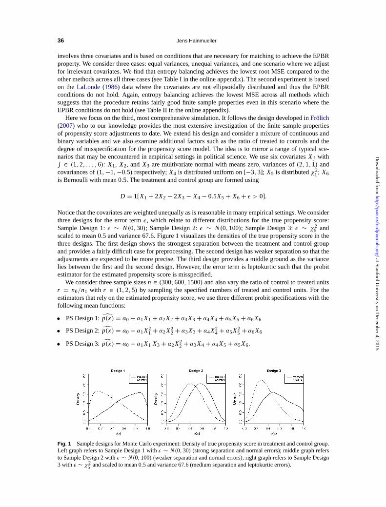
Here we focus on the third, most comprehensive simulation. It follows the design developed inFrolich(2007) who to our knowledge provides the most extensive investigation of the finite sample propertiesof propensity score adjustments to date. We extend his design and consider a mixture of continuous andbinary variables and we also examine additional factors such as the ratio of treated to controls and thedegree of misspecification for the propensity score model. The idea is to mirror a range of typical sce-narios that may be encountered in empirical settings in political science. We use six covariatesX j withj ∈ (1,2, . . . ,6): X1, X2, and X3 are multivariate normal with means zero, variances of(2,1,1) andcovariances of(1,−1,−0.5) respectively;X4 is distributed uniform on [−3,3]; X5 is distributedχ2
1 ; X6is Bernoulli with mean 0.5. The treatment and control group are formed using
D = 1[X1 + 2X2 − 2X3 − X4 − 0.5X5 + X6 + ε > 0].
Notice that the covariates are weighted unequally as is reasonable in many empirical settings. We considerthree designs for the error termε, which relate to different distributions for the true propensity score:Sample Design 1:ε ∼ N(0,30); Sample Design 2:ε ∼ N(0,100); Sample Design 3:ε ∼ χ2
5 andscaled to mean 0.5 and variance 67.6. Figure1 visualizes the densities of the true propensity score in thethree designs. The first design shows the strongest separation between the treatment and control groupand provides a fairly difficult case for preprocessing. The second design has weaker separation so that theadjustments are expected to be more precise. The third design provides a middle ground as the variancelies between the first and the second design. However, the error term is leptokurtic such that the probitestimator for the estimated propensity score is misspecified.
We consider three sample sizesn ∈ (300,600,1500)and also vary the ratio of control to treated unitsr = n0/n1 with r ∈ (1,2,5) by sampling the specified numbers of treated and control units. For theestimators that rely on the estimated propensity score, we use three different probit specifications with thefollowing mean functions:
• PS Design 1:p(x) = α0 + α1X1 + α2X2 + α3X3 + α4X4 + α5X5 + α6X6
• PS Design 2:p(x) = α0 + α1X21 + α2X2
2 + α3X3 + α4X24 + α5X2
5 + α6X6
• PS Design 3:p(x) = α0 + α1X1 X3 + α2X22 + α3X4 + α4X5 + α5X6.
Fig. 1 Sample designs for Monte Carlo experiment: Density of true propensity score in treatment and control group.Left graph refers to Sample Design 1 withε ∼ N(0,30) (strong separation and normal errors); middle graph refersto Sample Design 2 withε ∼ N(0,100)(weaker separation and normal errors); right graph refers to Sample Design3 with ε ∼ χ2
5 and scaled to mean 0.5 and variance 67.6 (medium separation and leptokurtic errors).
at Stanford University on D
ecember 4, 2015
http://pan.oxfordjournals.org/D
ownloaded from

Entropy Balancing for Causal Effects 37
Thesefunctions are designed to yield various degrees of misspecification of the propensity score model.For normalε (Sample Designs 1 and 2), the first model is correct, the second model is slightly misspec-ified, and the third model is heavily misspecified. The correlations between the true and the estimatedpropensity scores are 1, 0.8, and 0.3, respectively. For nonnormalε (Sample Design 3), all three are mis-specified, again with increasing levels of misspecification. Finally, we consider three outcome designs:
• Outcome Design 1:Y = X1 + X2 + X3 − X4 + X5 + X6 + η
• OutcomeDesign 2:Y = X1 + X2 + 0.2 X3 X4 −√
X5 + η
• OutcomeDesign 3:Y = (X1 + X2 + X5)2 + η
with η ∼ N(0,1). These regression functions are increasing in the degrees of nonlinearity in the mappingof the covariates to the outcome. The true treatment effect is fixed at zero for all units. The differentoutcomes also exhibit different correlations with the true propensity score decreasing from 0.8, 0.54, to0.16 from sample design 1 to 3, respectively. We run 1000 simulations and report the bias and root MSE.
4.2 Results
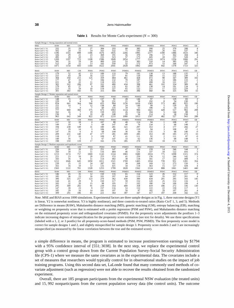
The full results for N = 300 are presented in Table1. To facilitate the interpretation, Figure2 alsopresents a graphical summary of the sampling distributions for the case of the 1:5 treated to control ratio.Full results forN = 600 andN = 1500 are reported in the web appendix. The results are fairly similaracross sample sizes.
Overall, the results suggest that entropy balancing outperforms the other adjustment techniques interms of MSE. This result is robust for all three sample designs, the three outcome specifications, thethree ratios of controls to treated, and the three propensity score equations. The gains in MSE are oftensubstantial. For example, in the most difficult case of sample design 1 (strong separation),N = 300, andthe highly nonlinear outcome design 3, the MSE from entropy balancing is about 2.6 times lower than thatof genetic matching, 3.4 times lower than pair matching on a propensity score that is estimated with thecorrectly specified probit regression, 3.9 times lower than Mahalanobis distance matching, and 4.6 timeslower than weighting on the estimated propensity score. As expected, we find that weighting or matchingon misspecified propensity scores (PS designs 2 and 3) results in much higher MSE even in large samples.
Entropy balancing also outperforms the other matching techniques in terms of bias, except in largersamples where matching and weighting on the propensity scores from the correctly specified probit modelsyield equally good bias performance as one would expect given that stochastic balancing of the covariatesimproves. Yet, in these cases, entropy balancing retains lower MSE even at a sample size ofN = 1500.This demonstrates the efficiency gains in finite samples that can be derived from adjusting the weightsdirectly to the known sample moments.
5 Empirical Applications
In this section, we illustrate the use of entropy balancing in two real data settings. The first illustrationreanalyzes data from a randomized evaluation of a large scale job training program. The second illustrationapplies the methods to a typical political science data set provided byLadd and Lenz(2009) who studythe effect of newspaper endorsements on vote choice in the 1997 British general election. Additionalillustrations are provided in the web appendix.
5.1 TheLaLonde Data
As a validation exercise, we first apply entropy balancing to theLaLonde(1986) data set, a canoni-cal benchmark in the causal inference literature (seeDiamond and Sekhon(2006) for the extensive de-bate surrounding this data set).15 TheLaLonde data consist of two parts. The first data set comes from arandomized evaluation of a large scale job training program, the National Supported Work Demonstra-tion (NSW). This experimental data provide a benchmark estimate for the effect of the program. Using
15Noticethat we focus on the Dehejia and Wahba subset of the LaLonde data.
at Stanford University on D
ecember 4, 2015
http://pan.oxfordjournals.org/D
ownloaded from
38 Jens Hainmueller
Table 1 Resultsfor Monte Carlo experiment (N= 300)
SampleDesign 1: Strong separation and normalerrors
MSE RAW MD GM PSM1 PSM2 PSM3 PSMD1 PSMD2 PSMD3 PSW1 PSW2 PSW3 EB
RatioCtoT 1 Y1 332 35 29 27 384 193 68 385 200 25 370 188 4RatioCtoT 1 Y2 502 24 15 14 163 532 71 193 442 26 161 537 5RatioCtoT 1 Y3 1196 1355 898 1186 1676 1835 2266 1995 2377 1590 1486 1633 346RatioCtoT 3 Y1 326 29 21 23 369 191 56 370 196 17 362 184 4RatioCtoT 3 Y2 495 20 10 11 155 523 57 175 445 18 157 528 4RatioCtoT 3 Y3 1269 1197 723 1108 1586 1849 2054 1777 2316 1074 1356 1666 291RatioCtoT 5 Y1 341 31 19 24 400 210 53 383 210 14 385 195 4RatioCtoT 5 Y2 512 20 12 13 165 550 52 172 473 15 166 547 5RatioCtoT 5 Y3 1471 1154 693 1184 1622 2041 2028 1892 2460 942 1378 1723 325
BIAS RAW MD GM PSM1 PSM2 PSM3 PSMD1 PSMD2 PSMD3 PSW1 PSW2 PSW3 EB
RatioCtoT 1 Y1 179 52 42 13 189 133 79 192 138 13 188 135 1RatioCtoT 1 Y2 222 43 29 16 122 227 81 134 208 15 122 230 3RatioCtoT 1 Y3 304 350 215 125 359 404 461 428 472 98 347 389 102RatioCtoT 3 Y1 177 47 33 7 184 132 70 187 136 12 186 133 -1RatioCtoT 3 Y2 221 38 22 11 118 225 71 127 208 16 121 227 1RatioCtoT 3 Y3 302 322 206 97 332 400 434 398 461 102 334 389 85RatioCtoT 5 Y1 179 45 27 9 189 135 65 187 138 14 191 134 0RatioCtoT 5 Y2 223 35 19 10 119 227 65 122 211 17 123 229 2RatioCtoT 5 Y3 301 302 182 75 315 400 416 396 460 90 325 384 55
SampleDesign 2: Weaker separation and normalerrorsMSE RAW MD GM PSM1 PSM2 PSM3 PSMD1 PSMD2 PSMD3 PSW1 PSW2 PSW3 EBRatioCtoT 1 Y1 148 15 8 12 137 91 28 146 97 7 129 83 2RatioCtoT 1 Y2 229 8 4 6 59 231 21 58 192 8 54 230 2RatioCtoT 1 Y3 654 661 364 590 655 994 1156 1016 1383 573 482 825 196RatioCtoT 3 Y1 151 14 7 12 138 89 24 140 99 5 130 82 2RatioCtoT 3 Y2 225 7 4 7 60 225 18 52 196 6 54 225 3RatioCtoT 3 Y3 777 660 360 575 673 1063 1114 984 1421 428 517 902 208RatioCtoT 5 Y1 162 16 7 19 159 103 26 154 104 5 144 88 3RatioCtoT 5 Y2 236 9 6 10 66 248 20 56 214 6 58 238 3RatioCtoT 5 Y3 963 642 349 822 872 1233 1080 1013 1507 482 527 943 288
BIAS RAW MD GM PSM1 PSM2 PSM3 PSMD1 PSMD2 PSMD3 PSW1 PSW2 PSW3 EBRatioCtoT 1 Y1 117 32 18 4 107 88 48 114 94 1 108 87 1RatioCtoT 1 Y2 149 19 9 5 69 147 40 70 134 2 68 148 2RatioCtoT 1 Y3 194 238 149 31 180 281 321 297 353 4 177 266 27RatioCtoT 3 Y1 117 29 14 3 106 86 43 110 94 3 108 87 -1RatioCtoT 3 Y2 147 16 6 4 68 144 36 64 135 3 68 146 -0RatioCtoT 3 Y3 209 231 140 47 177 281 309 285 353 39 185 273 33RatioCtoT 5 Y1 118 27 10 3 109 87 41 111 92 2 111 87 -0RatioCtoT 5 Y2 149 16 5 5 67 147 33 62 136 3 68 148 0RatioCtoT 5 Y3 198 210 119 17 165 276 285 270 341 18 174 263 5
SampleDesign 3: Medium separation and leptokurticerrorsMSE RAW MD GM PSM1 PSM2 PSM3 PSMD1 PSMD2 PSMD3 PSW1 PSW2 PSW3 EBRatioCtoT 1 Y1 226 26 20 23 251 147 47 254 159 14 246 144 3RatioCtoT 1 Y2 350 18 11 11 116 404 46 131 337 18 122 416 3RatioCtoT 1 Y3 1213 1174 757 1069 1143 1534 1983 1680 2024 775 1098 1315 374RatioCtoT 3 Y1 221 23 16 20 253 153 41 250 156 12 246 142 3RatioCtoT 3 Y2 343 16 9 11 114 402 38 118 341 17 122 408 3RatioCtoT 3 Y3 1212 1046 645 1050 1011 1521 1769 1465 1934 739 951 1281 354RatioCtoT 5 Y1 239 25 15 24 287 161 38 268 169 12 273 150 3RatioCtoT 5 Y2 355 16 10 12 125 421 34 118 363 15 127 428 4RatioCtoT 5 Y3 1563 1122 701 1328 1253 1799 1828 1562 2124 888 1061 1465 440
BIAS RAW MD GM PSM1 PSM2 PSM3 PSMD1 PSMD2 PSMD3 PSW1 PSW2 PSW3 EBRatioCtoT 1 Y1 146 45 35 12 150 116 65 154 123 26 152 117 0RatioCtoT 1 Y2 185 36 23 16 101 197 64 110 180 35 107 201 4RatioCtoT 1 Y3 306 325 217 123 270 362 430 390 434 201 295 343 145RatioCtoT 3 Y1 144 41 29 9 150 117 59 152 120 25 152 116 1RatioCtoT 3 Y2 183 32 20 15 98 195 57 102 180 34 106 199 4RatioCtoT 3 Y3 295 300 202 91 239 354 400 358 419 186 272 336 130RatioCtoT 5 Y1 147 39 23 9 157 116 53 153 122 22 159 117 1RatioCtoT 5 Y2 185 29 16 14 101 197 50 97 182 29 107 201 4RatioCtoT 5 Y3 309 291 186 85 221 364 387 347 417 187 268 342 122
Note.MSE and BIAS across 1000 simulations. Experimental factors are three sample designs as in Fig.1, three outcome designs (Y1is linear, Y2 is somewhat nonlinear, Y3 is highly nonlinear), and three controls-to-treated ratios (Ratio CtoT 1, 3, and 5). Methodsare Difference in means (RAW), Mahalanobis distance matching (MD), genetic matching (GM), entropy balancing (EB), matchingor weighting on propensity score that is estimated with a probit regression (PSM and PSW), and Mahalanobis distance matchingon the estimated propensity score and orthogonalized covariates (PSMD). For the propensity score adjustments the postfixes 1–3indicate increasing degrees of misspecification for the propensity score estimation (see text for details). We use three specifications(labeled with a 1, 2, or 3 postfix) for all propensity-score-based methods (PSM, PSW, PSMD). The first propensity score model iscorrect for sample designs 1 and 2, and slightly misspecified for sample design 3. Propensity score models 2 and 3 are increasinglymisspecified (as measured by the linear correlation between the true and the estimated score).
a simple difference in means, the program is estimated to increase postintervention earnings by $1794with a 95% confidence interval of [551; 3038]. In the next step, we replace the experimental controlgroup with a control group drawn from the Current Population Survey-Social Security Administrationfile (CPS-1) where we measure the same covariates as in the experimental data. The covariates include aset of measures that researchers would typically control for in observational studies on the impact of jobtraining programs. Using this second data set, LaLonde found that many commonly used methods of co-variate adjustment (such as regression) were not able to recover the results obtained from the randomizedexperiment.
Overall, there are 185 program participants from the experimental NSW evaluation (the treated units)and 15, 992 nonparticipants from the current population survey data (the control units). The outcome
at Stanford University on D
ecember 4, 2015
http://pan.oxfordjournals.org/D
ownloaded from

Entropy Balancing for Causal Effects 39
Fig
.2
Res
ults
ofM
onte
Car
loex
perim
ent.
Box
plot
svi
sual
ize
the
sam
plin
gdi
strib
utio
nof
1000
Mon
teC
arlo
estim
ates
from
the
vario
uspr
epro
cess
ing
met
hods
for
the
thre
eou
tcom
ede
sign
san
dth
ree
sam
ple
desi
gns
(with
a1:
5tr
eate
dto
cont
rolr
atio
N=
300)
.T
hetr
uetr
eatm
ent
effe
ctis
zero
(das
hed
vert
ical
line)
.M
etho
dsar
edi
ffere
nce
inm
eans
,M
ahal
anob
isdi
stan
cem
atch
ing,
gene
ticm
atch
ing,
entr
opy
bala
ncin
g,m
atch
ing
orw
eigh
ting
onpr
open
sity
scor
e(e
stim
ated
with
apr
obit
regr
essi
on),
and
Mah
alan
obis
dist
ance
mat
chin
gon
the
estim
ated
prop
ensi
tysc
ore
and
orth
ogon
aliz
edco
varia
tes.
For
the
prop
ensi
tysc
ore
adju
stm
ents
,th
epo
stfix
es1–
3in
dica
tein
crea
sing
degr
ees
ofm
issp
ecifi
catio
nfo
rth
epr
open
sity
scor
ees
timat
ion
(see
text
for
deta
ils).
at Stanford University on D
ecember 4, 2015
http://pan.oxfordjournals.org/D
ownloaded from
40 Jens Hainmueller
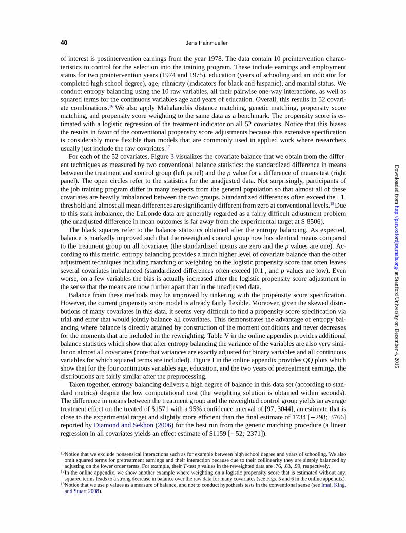
of interest is postintervention earnings from the year 1978. The data contain 10 preintervention charac-teristics to control for the selection into the training program. These include earnings and employmentstatus for two preintervention years (1974 and 1975), education (years of schooling and an indicator forcompleted high school degree), age, ethnicity (indicators for black and hispanic), and marital status. Weconduct entropy balancing using the 10 raw variables, all their pairwise one-way interactions, as well assquared terms for the continuous variables age and years of education. Overall, this results in 52 covari-ate combinations.16 We also apply Mahalanobis distance matching, genetic matching, propensity scorematching, and propensity score weighting to the same data as a benchmark. The propensity score is es-timated with a logistic regression of the treatment indicator on all 52 covariates. Notice that this biasesthe results in favor of the conventional propensity score adjustments because this extensive specificationis considerably more flexible than models that are commonly used in applied work where researchersusually just include the raw covariates.17
For each of the 52 covariates, Figure3 visualizes the covariate balance that we obtain from the differ-ent techniques as measured by two conventional balance statistics: the standardized difference in meansbetween the treatment and control group (left panel) and thep value for a difference of means test (rightpanel). The open circles refer to the statistics for the unadjusted data. Not surprisingly, participants ofthe job training program differ in many respects from the general population so that almost all of thesecovariates are heavily imbalanced between the two groups. Standardized differences often exceed the|.1|threshold and almost all mean differences are significantly different from zero at conventional levels.18Dueto this stark imbalance, the LaLonde data are generally regarded as a fairly difficult adjustment problem(the unadjusted difference in mean outcomes is far away from the experimental target at $-8506).
The black squares refer to the balance statistics obtained after the entropy balancing. As expected,balance is markedly improved such that the reweighted control group now has identical means comparedto the treatment group on all covariates (the standardized means are zero and thep values are one). Ac-cording to this metric, entropy balancing provides a much higher level of covariate balance than the otheradjustment techniques including matching or weighting on the logistic propensity score that often leavesseveral covariates imbalanced (standardized differences often exceed|0.1|, andp values are low). Evenworse, on a few variables the bias is actually increased after the logistic propensity score adjustment inthe sense that the means are now further apart than in the unadjusted data.
Balance from these methods may be improved by tinkering with the propensity score specification.However, the current propensity score model is already fairly flexible. Moreover, given the skewed distri-butions of many covariates in this data, it seems very difficult to find a propensity score specification viatrial and error that would jointly balance all covariates. This demonstrates the advantage of entropy bal-ancing where balance is directly attained by construction of the moment conditions and never decreasesfor the moments that are included in the reweighting. Table V in the online appendix provides additionalbalance statistics which show that after entropy balancing the variance of the variables are also very simi-lar on almost all covariates (note that variances are exactly adjusted for binary variables and all continuousvariables for which squared terms are included). Figure I in the online appendix provides QQ plots whichshow that for the four continuous variables age, education, and the two years of pretreatment earnings, thedistributions are fairly similar after the preprocessing.
Taken together, entropy balancing delivers a high degree of balance in this data set (according to stan-dard metrics) despite the low computational cost (the weighting solution is obtained within seconds).The difference in means between the treatment group and the reweighted control group yields an averagetreatment effect on the treated of $1571 with a 95% confidence interval of [97, 3044], an estimate that isclose to the experimental target and slightly more efficient than the final estimate of 1734 [−298; 3766]reported byDiamond and Sekhon(2006) for the best run from the genetic matching procedure (a linearregression in all covariates yields an effect estimate of $1159 [−52; 2371]).
16Noticethat we exclude nonsensical interactions such as for example between high school degree and years of schooling. We alsoomit squared terms for pretreatment earnings and their interaction because due to their collinearity they are simply balanced byadjusting on the lower order terms. For example, theirT-testp values in the reweighted data are.76, .83, .99, respectively.
17In the online appendix, we show another example where weighting on a logistic propensity score that is estimated without any.squared terms leads to a strong decrease in balance over the raw data for many covariates (see Figs. 5 and 6 in the online appendix).
18Noticethat we usep values as a measure of balance, and not to conduct hypothesis tests in the conventional sense (seeImai, King,and Stuart 2008).
at Stanford University on D
ecember 4, 2015
http://pan.oxfordjournals.org/D
ownloaded from
Entropy Balancing for Causal Effects 41
Fig. 3 Covariate balance in the LaLonde data. Left panel shows plot of covariate-by-covariate standardized biasin the unadjusted data and after the various preprocessing methods. The standardized bias measures the differencein means between the treatment and control group (scaled by the standard deviation). Zero bias indicates identicalmeans, dots to the right (left) of zero indicate a higher mean among the treatment (control) group. The right panelshows thep value for a covariate-by-covariatet-test for the differences in means after the unadjusted data and afterthe various preprocessing methods.
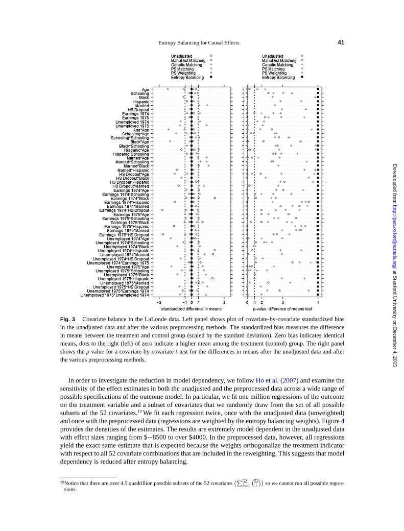
In order to investigate the reduction in model dependency, we followHo et al.(2007) and examine thesensitivity of the effect estimates in both the unadjusted and the preprocessed data across a wide range ofpossible specifications of the outcome model. In particular, we fit one million regressions of the outcomeon the treatment variable and a subset of covariates that we randomly draw from the set of all possiblesubsets of the 52 covariates.19 We fit each regression twice, once with the unadjusted data (unweighted)and once with the preprocessed data (regressions are weighted by the entropy balancing weights). Figure4provides the densities of the estimates. The results are extremely model dependent in the unadjusted datawith effect sizes ranging from $−8500 to over $4000. In the preprocessed data, however, all regressionsyield the exact same estimate that is expected because the weights orthogonalize the treatment indicatorwith respect to all 52 covariate combinations that are included in the reweighting. This suggests that modeldependency is reduced after entropy balancing.
19Notice that there are over 4.5 quadrillion possible subsets of the 52 covariates(∑52
i =1(52
i))
so we cannot run all possible regres-sions.
at Stanford University on D
ecember 4, 2015
http://pan.oxfordjournals.org/D
ownloaded from

42 Jens Hainmueller
Fig. 4 Model dependency in the LaLonde data. Density of estimated treatment effects across one million randomlysampled model specifications in the unadjusted data (solid) and the data preprocessed with entropy balancing (dashedline).
5.2 News Media Persuasion
In this section, we apply entropy balancing to a typical political science survey data set by reanalyzing datafrom Ladd and Lenz(2009) who examine how shifts in the partisan endorsements of British newspapersaffected major party vote choice in the 1997 general election.20 The authors’ identification strategy exploitsthe fact that on the second day of the official election campaign, theSun(which had the largest circulationin Great Britain) and several other British newspapers ended their long-standing support for the rulingConservative party and switched their endorsement to the Labour candidate Tony Blair.Ladd and Lenz(2009) draw upon data from several waves of the British Election Panel Study 1992–1997, where the samevoters are being interviewed before the endorsement shifts (in 1992, 1994, 1995, and 1996) and oncefollowing the 1997 election. The main comparison involves 211 “treated” respondents who in 1996 (thelast wave before the shifts in endorsements) report that they read one of the newspapers that eventuallyswitched their endorsement to Labour prior to the 1997 election. These treated voters are compared to1382 “control” respondents who either read papers whose partisan endorsements remained constant orwho report that they did not read a paper. The outcome variable is vote choice in the 1997 election asreported in the postelection survey.
The authors control for a battery of pretreatment variables to account for the nonrandom selection intoreadership of switching newspapers. The control variables include various measures for a respondent’sprior evaluation of the Labour Party (such as prior party support, prior labour vote, etc.), prior ideology,socioeconomic status, authoritarianism, gender, age, region, and occupation.21 There are 39 covariatesoverall; most of them are binary or ordinal. In their analysis, the authors rescale all variables to vary fromzero to one, match on a subset of eight of the most important covariates, and finally include the additionalcontrols in a subsequent regression of the outcome on the treatment indicator and all control variables inthe preprocessed data. We conduct entropy balancing by imposing moment conditions on the means of allcovariates directly. Since most variables are binary, exactly adjusting the means also exactly adjusts thevariances. We also apply the other adjustment methods to the same data; the propensity score is estimatedwith a logistic regression in all 39 covariates.
Figure5 displays the balance results from the various preprocessing methods as measured by the stan-dardized differences in means (left panel) and thep values of the difference in means tests (right panel).
20I am grateful to the authors for sharing their data.21Notice that variables that are labeled as “prior” are measured in the 1992–1996 survey waves. See the authors’ web appendix for
a detailed explanation of the variable definitions.
at Stanford University on D
ecember 4, 2015
http://pan.oxfordjournals.org/D
ownloaded from
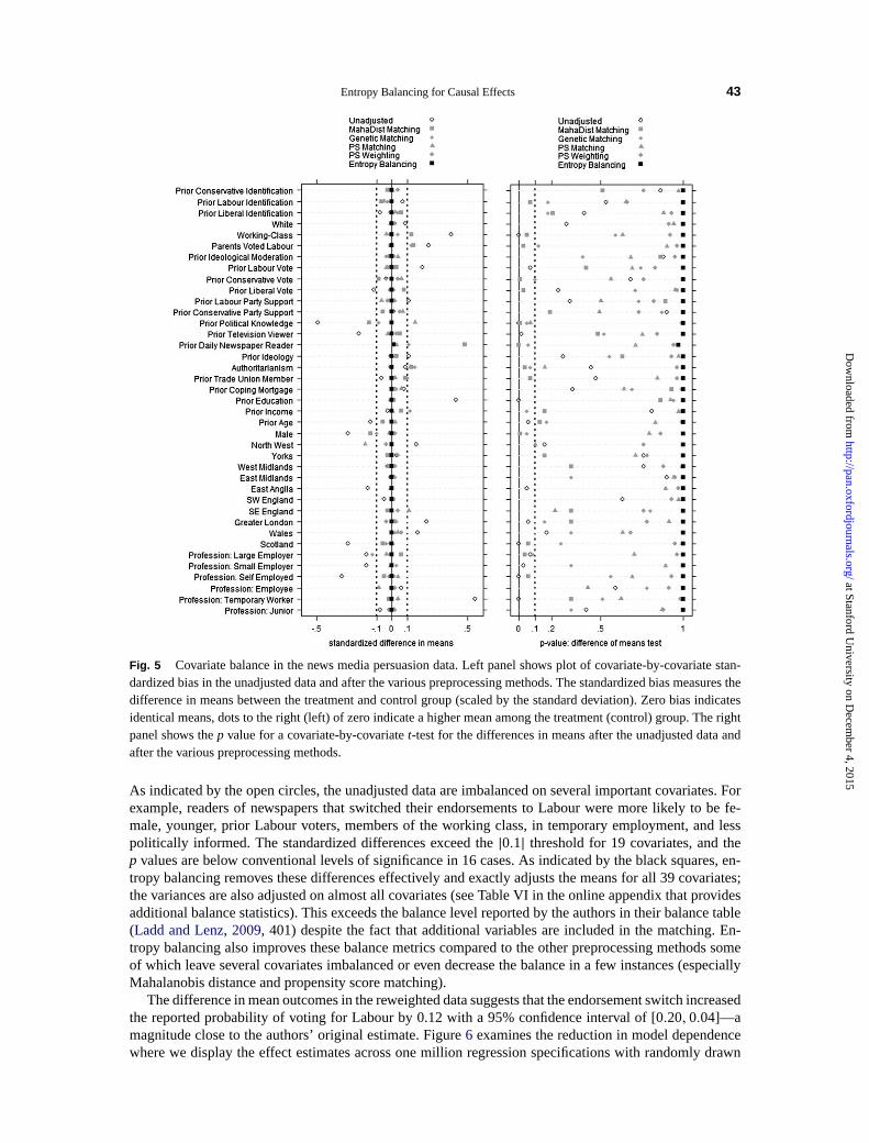
Entropy Balancing for Causal Effects 43
Fig. 5 Covariate balance in the news media persuasion data. Left panel shows plot of covariate-by-covariate stan-dardized bias in the unadjusted data and after the various preprocessing methods. The standardized bias measures thedifference in means between the treatment and control group (scaled by the standard deviation). Zero bias indicatesidentical means, dots to the right (left) of zero indicate a higher mean among the treatment (control) group. The rightpanel shows thep value for a covariate-by-covariatet-test for the differences in means after the unadjusted data andafter the various preprocessing methods.
As indicated by the open circles, the unadjusted data are imbalanced on several important covariates. Forexample, readers of newspapers that switched their endorsements to Labour were more likely to be fe-male, younger, prior Labour voters, members of the working class, in temporary employment, and lesspolitically informed. The standardized differences exceed the|0.1| threshold for 19 covariates, and thep values are below conventional levels of significance in 16 cases. As indicated by the black squares, en-tropy balancing removes these differences effectively and exactly adjusts the means for all 39 covariates;the variances are also adjusted on almost all covariates (see Table VI in the online appendix that providesadditional balance statistics). This exceeds the balance level reported by the authors in their balance table(Ladd and Lenz, 2009, 401) despite the fact that additional variables are included in the matching. En-tropy balancing also improves these balance metrics compared to the other preprocessing methods someof which leave several covariates imbalanced or even decrease the balance in a few instances (especiallyMahalanobis distance and propensity score matching).
The difference in mean outcomes in the reweighted data suggests that the endorsement switch increasedthe reported probability of voting for Labour by 0.12 with a 95% confidence interval of [0.20,0.04]—amagnitude close to the authors’ original estimate. Figure6 examines the reduction in model dependencewhere we display the effect estimates across one million regression specifications with randomly drawn
at Stanford University on D
ecember 4, 2015
http://pan.oxfordjournals.org/D
ownloaded from

44 Jens Hainmueller
Fig. 6 Model dependency in the news media persuasion data. Density of estimated treatment effects across onemillion randomly sampled model specifications in the unadjusted data (solid) and the data preprocessed with entropybalancing (dashed line).
covariate subsets in the raw and the preprocessed data. The effect estimates remain stable in the prepro-cessed data since the entropy balancing weights orthogonalize the treatment indicator to all covariates.In the raw data, the effects vary from about 0.06 to 0.18 across the different regressions suggesting thatmodel dependence is considerably lower after the preprocessing.
6 Conclusion
The goal of preprocessing is to generate well-balanced samples, but commonly used methods often make itdifficult for applied researchers to achieve high balance targets. One reason for this is that many commonlyused methods fail to focus on covariate balance directly, but instead rely on an intricate and often ineffec-tive process of “manually” iterating between propensity score modeling, matching, and balance checkingto search for a suitable balancing solution. In the worst case, these techniques may increase bias for thesubsequent estimation of treatment effects when balance improvements in some covariates are accompa-nied with decreased balance for other important covariates.
We propose entropy balancing as a processing technique to create balanced samples. In entropy bal-ancing, the researcher starts by imposing a potentially large set of balance conditions which imply that thetreatment and reweighted control group match exactly on a possibly large set of the prespecified moments.Entropy balancing then directly adjusts the unit weights to the specified sample moments while movingthe weights as little as possible to retain information. This makes it easier for the user to find unit weightsthat balance the moments between the treatment and control group and obviates the need for continualbalance checking for the moments that are included in the reweighting.
The entropy balancing weights can be paired with standard estimators that the researcher may wantto use to subsequently model the outcome in the preprocessed data. The balance improvements that re-sult from entropy balancing can translate into lower approximation error and reduced model dependencyin finite samples as demonstrated through the extensive Monte Carlo simulations and several empiricalapplications. Future research may consider the combination of entropy balancing and other preprocessingmethods.
While entropy balancing simplifies the search for covariate balance for practitioners, it is importantto notice that other problems that are commonly associated with preprocessing methods (and covariateadjustment more generally) still apply. For example, entropy balancing provides no safeguard against biasfrom unmeasured confounders that are often a vexing problem in observational studies.
at Stanford University on D
ecember 4, 2015
http://pan.oxfordjournals.org/D
ownloaded from

Entropy Balancing for Causal Effects 45
References
Abadie,A., and G. Imbens. 2007. Simple and bias-corrected matching estimators for average treatment effects. Working Paper.Harvard University.
Brookhart, M., S. Schneeweiss, K. Rothman, R. Glynn, J. Avorn, and T. Sturmer. 2006. Variable selection for propensity scoremodels.American Journal of Epidemiology163:1149–56.
DellaVigna, S., and E. Kaplan. 2007. The Fox News effect: Media bias and voting.Quarterly Journal of Economics122:1187–34.Deming, W., and F. Stephan. 1940. On the least squares adjustment of a sampled frequency table when the expected marginal totals
are known.The Annals of Mathematical Statistics11:427–44.Diamond, A. J., and J. Sekhon. 2006. Genetic matching for causal effects: A general multivariate matching method for achieving
balance in observational studies. Unpublished manuscript, Department of Political Science, UC Berkeley.Drake, C. 1993. Effects of misspecification of the propensity score on estimators of treatment effect.Biometrics49:1231–36.Eggers, A., and J. Hainmueller. 2009. MPs for sale? Returns to office in postwar British politics.American Political Science Review
103:513–33.Erlander, S. 1977.Entropy in linear programs–an approach to planning. Report No. LiTH-MAT-R-77-3. Department of Mathemat-
ics, Linkoping University, Sweden.———. 2004. Finite sample properties of propensity-score matching and weighting estimators.Review of Economics and Statistics
86:77–90.Frolich, M. 2007. Propensity score matching without conditional independence assumption with an application to the gender wage
gap in the United Kingdom.The Econometrics Journal10:359–407.Graham, B. S., C. Pinto, and D. Egel. 2010. Inverse probability tilting for moment condition models with missing data. Working
paper. New York University.Gu, X., and P. Rosenbaum. 1993. Comparison of multivariate matching methods: Structures, distances, and algorithms.Journal of
Computational and Graphical Statistics2:405–20.Hahn, J. 1998. On the role of the propensity score in efficient semiparametric estimation of average treatment effects.Econometrica
66:315–31.Hansen, B. B., and J. Bowers. 2008. Covariate balance in simple, stratified and clustered comparative studies.Statistical Science
23:219–36.Hansen, L. 1982. Large sample properties of generalized method of moments estimators.Econometrica50:1029–54.Hellerstein, J., and G. Imbens. 1999. Imposing moment restrictions from auxiliary data by weighting.The Review of Economics and
Statistics81:1–14.Hirano, K., and G. Imbens. 2001. Estimation of causal effects using propensity score weighting: An application of data on right hear
catherization.Health Services and Outcomes Research Methodology2:259–78.Hirano, K., G. Imbens, and G. Ridder. 2003. Efficient estimation of average treatment effects using the estimated propensity score.
Econometrica71:1161–89.Ho, D., K. Imai, G. King, and E. Stuart. 2007. Matching as nonparametric preprocessing for reducing model dependence in para-
metric causal inference.Political Analysis15:199–236.Horvitz, D., and D. Thompson. 1952. A generalization of sampling without replacement from a finite universe.Journal of the
American Statistical Association47:663–85.Iacus, S., G. King, and G. Porro. 2009.Causal inference without balance checking: Coarsened exact matching. Mimeo Harvard
University.Imai, K., G. King, and E. Stuart. 2008. Misunderstandings among experimentalists and observationalists: Balance test fallacies in
causal inference.Journal of the Royal Statistical Society, Series A171:481–502.Imbens, G. 1997. One-step estimators for over-identified generalized method of moments models.The Review of Economic Studies
64:359–83.———. 2004. Nonparametric estimation of average treatment effects under exogeneity: A review.Review of Economics and Statis-
tics86:4–29.Imbens, G., R. Spady, and P. Johnson. 1998. Information theoretic approaches to inference in moment condition models.Economet-
rica 66:333–57.Ireland, C., and S. Kullback. 1968. Contingency tables with given marginals.Biometrika55:179–88.Kapur, J., and H. Kevsavan. 1992.Entropy optimization principles with applications. London: Academic Press.Kitamura, Y., and M. Stutzer. 1997. An information-theoretic alternative to generalized method of moments estimation.Economet-
rica 65:861–74.Kullback, S. 1959.Information theory and statistics. New York: Wiley.Ladd, J., and G. Lenz. 2009. Exploiting a rare communication shift to document the persuasive power of the news media.American
Journal of Political Science53:394–10.LaLonde, R. J. 1986. Evaluating the econometric evaluations of training programs with experimental data.American Economic
Review76:604–20.Mattos, R., and A. Veiga. 2004. Entropy optimization: Computer implementation of the maxent and minexent principles. Working
Paper. Universidade Federal de Juiz de Fora, Brazil.McCaffrey, D., G. Ridgeway, and A. Morral. 2004. Propensity score estimation with boosted regression for evaluating adolescent
substance abuse treatment.Psychological Methods9:403–25.Oh, H. L., and F. J. Scheuren. 1978. Multivariate ratio raking estimation in the 1973 exact match study.Proceedings of the Section
on Survey Research MethodsXXV:716–22.Owen, A. 2001.Empirical likelihood. Boca Raton, FL: Chapman & Hall.
at Stanford University on D
ecember 4, 2015
http://pan.oxfordjournals.org/D
ownloaded from

46 Jens Hainmueller
Qin, J., and J. Lawless. 1994. Empirical likelihood and general estimating equations.Annals of Statistics22:300–25.Qin, J., B. Zhang, and D. Leung. 2009. Empirical likelihood in missing data problems.Journal of the American Statistical Associa-
tion 104:1492–503.Read, T., and N. Cressie. 1988.Goodness-of-fit statistics for discrete multivariate data. New York: Springer.Robins, J., A. Rotnitzky, and L. Zhao. 1995. Analysis of semiparametric regression models for repeated outcomes in the presence
of missing data.Journal of the American Statistical Association90:106–21.Rosenbaum, P. R., and D. B. Rubin. 1983. The central role of the propensity score in observational studies for causal effects.
Biometrika70:41–55.Rubin, D. 2006.Matched sampling for causal effects. Cambridge: Cambridge University Press.Sarndal, C. E., and S. Lundstrom. 2006.Estimation in surveys with nonresponse. New York: John Wiley & Sons, Ltd.Schennach, S. 2007. Point estimation with exponentially tilted empirical likelihood.The Annals of Statistics35:634–72.Sekhon, J. 2006. Alternative balance metrics for bias reduction in matching methods for causal inference. Unpublished manuscript,
Department of of Political Science, UC Berkeley.Sekhon, J. S. 2009. Opiates for the matches: Matching methods for causal inference.Annual Review of Political Science12:487-08.Smith, J., and P. Todd. 2001. Reconciling conflicting evidence on the performance of propensity-score matching methods.American
Economic Review91:112–18.Zaslavsky, A. 1988. Representing local reweighting area adjustments by of households.Survey Methodology14:265–88.Zhao, Z. 2004. Using matching to estimate treatment effects: Data requirements, matching metrics, and Monte Carlo evidence.
Review of Economics and Statistics86:91–107.
at Stanford University on D
ecember 4, 2015
http://pan.oxfordjournals.org/D
ownloaded from