enhancing the economics of satellite constellations via...

1

• Massachusetts Institute of Technology• Space Systems Laboratory

Enhancing the Economics of Satellite Constellations via Staged Deployment

Prof. Olivier de Weck, Prof. Richard de NeufvilleMathieu Chaize

ESD.71 Engineering Systems Analysis for DesignGuest Lecture

December 4, 2003

- A Real Options Application -

12-4-2003ESD.71 Engineering Systems Analysis for Design 2

Outline

• Motivation• Traditional Approach• Conceptual Design

(Trade) Space Exploration

• Staged Deployment• Path Optimization for

Staged Deployment• Conclusions

Stage I21 satellites

3 planesh=2000 km

Stage II50 satellites

5 planesh=800 km

Stage III112 satellites

8 planesh=400 km

2


Motivation• Iridium was a technical success but an economic failure:

– 6 millions customers expected (1991)– Iridium had only 50 000 customers after 11 months of service (1998)

• The forecasts were wrong, primarily because they underestimated the market for terrestrial cellular telephones:

• Globalstar was deployed about a year later and also had to file for Chapter 11 protection

0

20

40

60

80

100

120

1991 1992 1993 1994 1995 1996 1997 1998 1999 2000

Year

Mill

ions

of s

ubsc

riber

s

US (forecast) US (actual)


Traditional Approach

• Decide what kind of service should be offered• Conduct a market survey for this type of service• Derive system requirements• Define an architecture for the overall system• Conduct preliminary design• Obtain FCC approval for the system• Conduct detailed design analysis and optimization• Implement and launch the system• Operate and replenish the system as required• Retire once design life has expired

3


Existing Big LEO Systems

Bankrupt but in operation

Bankrupt but in operation

Current Status(2003)

1414780Altitude (km)

$ 3.3 billion$ 5.7 billionTotal System Cost

2.4/4.8/9.6 kbps4.8 kbpsAverage Data Rate per Channel

voice and datavoice and dataType of Service

2,500 duplex channels120,000 channels

1,100 duplex channels72,600 channels

Single Satellite CapacityGlobal Capacity Cs

Multi-frequency –Code Division Multiple

Access

Multi-frequency – Time Division Multiple

Access

Multiple Access Scheme

380400Transmitter Power (W)

450689Sat. Mass (kg)

WalkerpolarConstellation Formation

4866Number of Sats.

1998 – 19991997 – 1998Time of Launch

GlobalstarIridium

IndividualIridium Satellite

IndividualGlobalstar Satellite


Satellite System Economics

,1

,1

1100

365 24 60

T T

ops ii

T

s f ii

kI CCPF

C L

=

=

+ + =

⋅ ⋅ ⋅ ⋅

∑

∑

Lifecycle cost

Number of billable minutes

Cost per function [$/min]Initial investment cost [$]Yearly interest rate [%]Yearly operations cost [$/y]Global instant capacity [#ch]Average load factor [0…1]Number of subscribersAverage user activity [min/y]Operational system life [y]

365 24 60min1.0

u u

sf

N ACL

⋅ ⋅ ⋅ ⋅=

CPFIkopsCsCfLuNuA

1, 200 [min/y]uA =

TNumerical Example:

0.20 [$/min]CPF =

3 [B$]I =5 [%]k =300 [M$/y]opsC =

100,000 [#ch]sC =63 10uN = ⋅ 0.068fL =

15 [y]T =

But with 50,000uN =

12.02 [$/min]CPF =Non-competitive

4


Conceptual Design (Trade) Space

Can we quantify the conceptual system design problem using simulation and optimization?

Simulator

Design(Input) Vector

Performance CapacityCost


Design (Input) Vector X

• The design variables are:– Constellation Type: C– Orbital Altitude: h– Minimum Elevation Angle: εmin

– Satellite Transmit Power: Pt

– Antenna Size: Da

– Multiple Access Scheme MA:– Network Architecture: ISL

Design Space

[-]yes, no

[-]MF-TDMA, MF-CDMA

[m]1.0,2.0,3.0

[W]200,400,800,1600,2400

[deg]2.5,7.5,12.5

[km]500,1000,1500,2000

Polar, Walker

This results in a 1440full factorial, combinatorialconceptual design space

Astro-dynamics

SatelliteDesign

C: 'walker'h: 2000

emin: 12.5000Pt: 2400DA: 3MA: 'MFCD'

ISL: 0

X1440=

Network

5


Objective Vector (Output) J

• Performance (fixed)– Data Rate per Channel: R=4.8 [kbps]– Bit-Error Rate: pb=10-3

– Link Fading Margin: 16 [dB]

• Capacity– Cs: Number of simultaneous duplex channels– Clife: Total throughput over life time [min]

• Cost– Lifecycle cost of the system (LCC [$]), includes:

• Research, Development, Test and Evaluation (RDT&E)• Satellite Construction and Test• Launch and Orbital Insertion• Operations and Replenishment

– Cost per Function, CPF [$/min]

Consider

Cs: 1.4885e+005Clife: 1.0170e+011

LCC: 6.7548e+009CPF: 6.6416e-002

J1440=


Multidisciplinary Simulator Structure

Constellation

SatelliteNetwork

LinkBudget

Spacecraft CostLaunchModule

Capacity

InputVector

ConstantsVector

OutputVector

x p

J

satm

Note: Only partial input-output relationships shown

min,h ε

,T p nGWspotn

sR sCLCC

, ,t aP D MA

ISL

satm

LV

satm Satellite MassT Number of Satellitesp Number of orbital planes

spotn Number of spot beamsnGW Number of gatewaysLV Launch vehicle selection

6


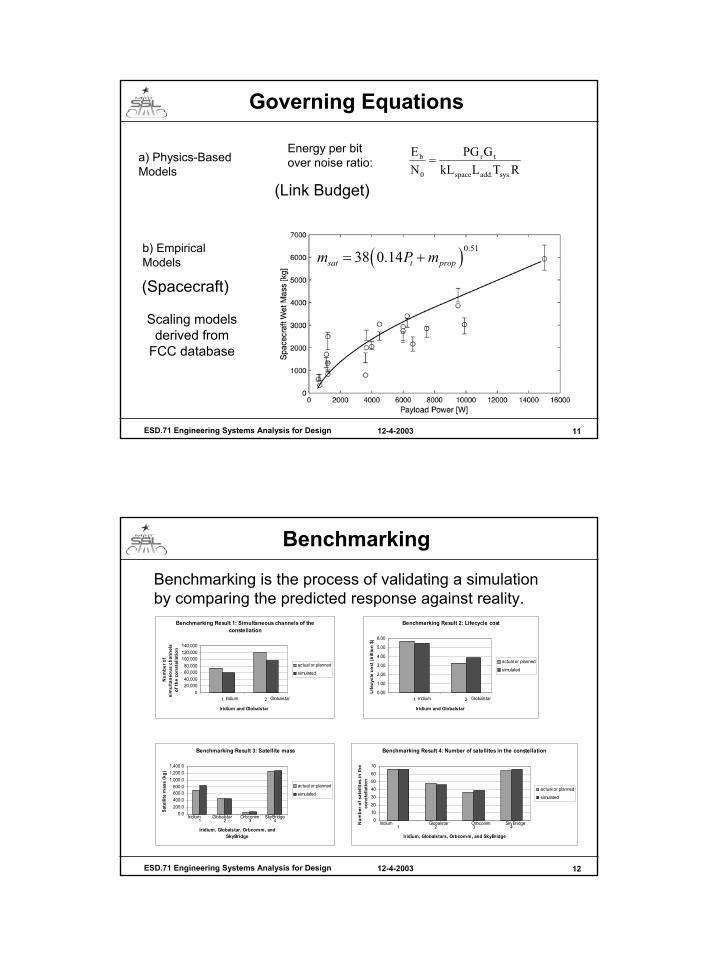
Governing Equations

a) Physics-Based Models RTLkL

GPGNE

sys.add.space

tr

0

b =Energy per bit over noise ratio:

(Link Budget)

b) Empirical Models

(Spacecraft)

( )0.5138 0.14sat t propm P m= +

Scaling modelsderived from

FCC database


Benchmarking

Benchmarking is the process of validating a simulationby comparing the predicted response against reality.

Benchmarking Result 1: Simultaneous channels of the constellation

020,00040,00060,00080,000

100,000120,000140,000

1 2

Iridium and Globalstar

Num

ber o

f si

mul

tane

ous

chan

nels

of

the

cons

tella

tion

actual or planned

simulated

Iridium Globalstar

Benchmarking Result 3: Satellite mass

0.0200.0400.0600.0800.0

1,000.01,200.01,400.0

1 2 3 4

Iridium, Globalstar, Orbcomm, and SkyBridge

Sate

llite

mas

s (k

g)

actual or planned

simulated

Iridium Globalstar Orbcomm SkyBridge

Benchmarking Result 2: Lifecycle cost

0.00

1.00

2.00

3.00

4.00

5.00

6.00

1 2

Iridium and Globalstar

Life

cycl

e co

st (b

illio

n $)

actual or planned

simulated

Iridium Globalstar

Benchmarking Result 4: Number of satellites in the constellation

010203040506070

1 2 3 4

Iridium, Globalstars, Orbcomm, and SkyBridge

Num

ber o

f sat

ellit

es in

the

cons

tella

tion

actual or planned

simulated

Iridium Globalstar Orbcomm SkyBridge

7


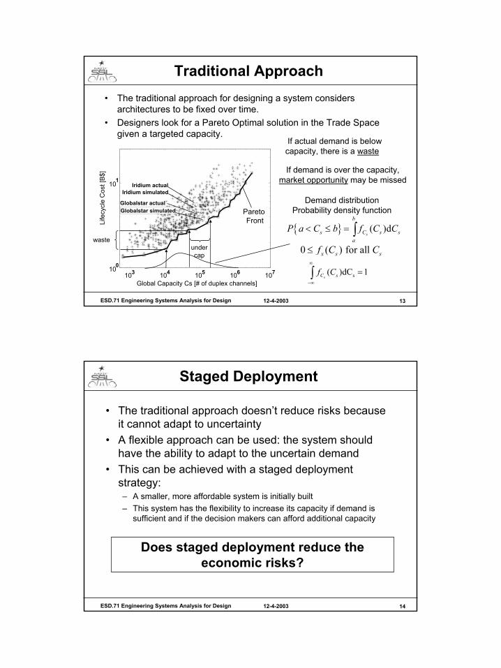
Traditional Approach• The traditional approach for designing a system considers

architectures to be fixed over time.• Designers look for a Pareto Optimal solution in the Trade Space

given a targeted capacity.

103 104 105 106 107100

101

Global Capacity Cs [# of duplex channels]

Life

cycl

e C

ost [

B$]

Iridium simulatedIridium actual

Globalstar simulatedGlobalstar actual

Pareto Front

If actual demand is below capacity, there is a waste

wasteundercap

If demand is over the capacity, market opportunity may be missed

s( )dC 1sC sf C

∞

−∞

=∫

Demand distributionProbability density function

0 ( ) for all x s sf C C≤

{ } ( )ds

b

s C s sa

P a C b f C C< ≤ = ∫


Staged Deployment

• The traditional approach doesn’t reduce risks because it cannot adapt to uncertainty

• A flexible approach can be used: the system should have the ability to adapt to the uncertain demand

• This can be achieved with a staged deployment strategy:– A smaller, more affordable system is initially built– This system has the flexibility to increase its capacity if demand is

sufficient and if the decision makers can afford additional capacity

Does staged deployment reduce the economic risks?

8


Economic Advantages

• The staged deployment strategy reduces the economic risks via two mechanisms

• The costs of the system are spread through time:– Money has a time value: to spend a dollar tomorrow is better

than spending one now (Present Value)– Delaying expenditures always appears as an advantage

• The decision to deploy is done observing the market conditions:– Demand may never grow and we may want to keep the system

as it is without deploying further.– If demand is important enough, we may have made sufficient

profits to invest in the next stage.

How to apply staged deployment to LEO constellations?


Proposed New Process

• Decide what kind of service should be offered• Conduct a market survey for this type of service• Conduct a baseline architecture trade study• Identify Interesting paths for Staged Deployment• Select an Initial Stage Architecture (based on Real Options

Analysis)• Obtain FCC approval for the system• Implement and Launch the system• Operate and observe actual demand• Make periodic reconfiguration decisions• Retire once Design Life has expired

∆t

Focus shifts from picking a “best guess” optimalarchitecture to choosing a valuable, flexible path

9


Step 1: Partition the Design Vector

– Constellation Type: C– Orbital Altitude: h– Minimum Elevation Angle: εmin

– Satellite Transmit Power: Pt

– Antenna Size: Da

– Multiple Access Scheme MA:– Network Architecture: ISL

Astro-dynamics

SatelliteDesign

C: 'walker'h: 2000

emin: 12.5000Pt: 2400DA: 3MA: 'MFCD'

ISL: 0

Network

xflexible

xbase

Rationale:Keep satellitesthe same andchange onlyarrangement

in space

Stage IC: 'polar'h: 1000

emin: 7.5000Pt: 2400DA: 3MA: 'MFCD'

ISL: 0

Stage II

xIbase xII

base=


Step 2: Search Paths in the Trade Space

Constant:

Pt=200 W

DA=1.5 m

ISL= Yes

Life

cycl

e co

st [B

$]

System capacity

h= 2000 kmε= 5 degNsats=24





family

10


Choosing a path: Valuation

• We want to see the adaptation of a path to market conditions:– How to mathematically represent the fact that demand is uncertain?– Usual valuation methods try to minimize costs and will recommend not

to deploy after the initial stage

• We don’t know how much it costs to achieve reconfiguration:– The technical method that will be used is not well known

• onboard propellant, space tug, refueling/servicer– Even if a method was identified, the pricing process may be long– Focus on the value of flexibility (“economic opportunity”)

• Many paths can be followed from an initial architecture:– Optimization over initial architectures seems difficult– Many cases will have to be considered


Assumptions

• Optimization is done over paths instead of initial architectures:• The capability to reconfigure the constellation is seen as a ``real

option’’ we want to price:– We have the right but not the obligation to use this flexibility– We don’t know the price for it but want to see if it gives an economic

opportunity– The difference of costs with a traditional design will give us the maximum price

we should be willing to pay for this option

• Demand follows a geometric Brownian motion:– Demand can go up or down between two decision points– Several scenarios for demand are generated based on this model

• The constellation adapts to demand:– If demand goes over capacity, we deploy to the next stage– This corresponds to a worst-case for staged deployment– In reality, adaptation to demand may not maximize revenues but if an

opportunity is revealed with the worst-case, a further optimization can be done

S t tS

µ σε∆= ∆ + ∆

S -stock price∆t – time period

ε- SND random variableµ, σ - constants

11


Step 3: Model Uncertain Demand• The geometric Brownian motion can be simplified with

the use of the Binomial model (see Lattice method):

• A scenario corresponds to a series of up and down movements such as the one represented in red

p

1-p


Step 4: Calculations of costs

• We compute the costs of a path with respect to each demand scenario

• We then look at the weighted average for cost over all scenarios

• We adapt to demand to study the ``worst-case’’ scenario

• The costs are discounted: the present value is considered

Cap1

Cap2

Costs

Initial deployment Reconfiguration

12


Step 5: Identify optimal path

102 103 104

100

101

Capacity [thousands of users]

Sys

tem

Lif

ecyc

le C

ost

[B$]

1.36

2.01

Best Path

A1

A2

A3

A4

• For a given targeted capacity, we compare our solution to the traditional approach

• Our approach allows important savings (30% on average)

• An economic opportunity for reconfigurations is revealed but the technical way to do it has to be studied

Traditional design

Staged Deployment Strategy

,maxsC( )

1( )

j

ni

j i pathi

E LCC path p LCC scenario=

= ∑


Framework: Summary

Identify Flexibility Generate “Paths” Model Demand

x =

xflex

xbase

Estimate CostsOptimize over PathsReveal opportunity

102 103 104

100

101

Capacity [thousands of users]

Sys

tem

Lif

ecyc

le C

ost

[B$]

1.36

2.01

Best Path

A1

A2

A3

A4

13


Staged Deployment FrameworkDefine parameters

IdentifyFeasible

Paths

GenerateDemand

Scenarios

Determinextrad

Minimize architecture pathsover lifecycle costs

Compare and find Economic Opportunity

Capmax

CapmaxCapmin

Cap(xtrad)

paths

Tsys

t

D,P

LCC*,path*LCC(xtrad)

IDC,OM, C

x,LCCNch

x,LCCNch


Conclusions

• The goal is not to rewrite the history of LEO constellations but to identify future opportunities

• We designed a framework to reveal economic opportunities for staged deployment strategies– Inspired by Real Options approach

• The method is general enough to be applied to similar design problems

• Reconfiguration needs to be studied in detail and many issues have to be solved:– Estimate ∆V and transfer time for different propulsion systems– Study the possibility of using a Tug to achieve reconfiguration– Response time– Service Outage

14


An Architectural Principle

Economic Benefits and risk reduction for large engineering systems can be shown by designing for staged

deployment, rather then for worst case, fixed capacity.

Embedding such flexibility does not come for free and evolution paths of system designs do not generally

coincide with the Pareto frontier.

enhancing the economics of satellite constellations via...

Documents