enhancing the performance of tcp over satellite links
TRANSCRIPT

Enhancing the Performance of TCP over Satellite
Links
by
Sonia Jain
Submitted to the Department of Electrical Engineering and ComputerScience
in partial fulfillment of the requirements for the degree of
Masters of Science in Electrical Engineering and Computer Science
at the
MASSACHUSETTS INSTITUTE OF TECHNOLOGY
June 2003
© Sonia Jain, MMIII. All rights reserved.
The author hereby grants to MIT permission to reproduce anddistribute publicly paper and electronic copies of this thesis document
in whole or in part. I MASSACHUSET
Author ................................... ..........................Department of Electrical Engineering and Computer Science
May 21, 2003
Certified by.. ........ ..............Eytan Modiano
Assistant ProfessorThesis Supervisor
A ccepted by ......... .. ..................Arthur C. Smith
Chairman, Department Committee on Graduate Students
BARKER
S INSTITUTEOF TECHNOLOGY
JUL 0 ' 2003
LIBRARIES

2

Enhancing the Performance of TCP over Satellite Links
by
Sonia Jain
Submitted to the Department of Electrical Engineering and Computer Scienceon May 21, 2003, in partial fulfillment of the
requirements for the degree ofMasters of Science in Electrical Engineering and Computer Science
Abstract
Understanding the interaction between TCP and MAC layer protocols in satellitenetworks is critical to providing high levels of service to users. We separate ourstudy of TCP and MAC layer protocols into two parts. We consider the problem ofscheduling at bottleneck links and propose two new queue management algorithms.They are capable of offering higher levels of fairness as well as lower latencies ina variety of scenarios. We also consider the problem of random access in satellitenetworks and its effect on the functionality of TCP.
We propose two queue management schemes: the Shortest Window First (SWF)and the Smallest Sequence Number First (SSF) with Approximate Longest QueueDrop. Our schedulers transmit short messages with minimal delay. The SWF sched-uler transmits short messages with low delay without increasing the delay experiencedby long messages, provided that short messages do not make up the majority of theload. Our schedulers show increased fairness over other commonly used schedulerswhen traffic is not homogeneous. They provide higher levels of throughput to isolatedmisbehaving (high propagation delays or error rates) sessions.
We consider the performance of TCP over random access channels. Researchershave extensively studied TCP and random access protocols, specifically ALOHA,individually. However, little progress has been made in understanding their combinedperformance. Through simulation, we explore the relationship between TCP andALOHA parameters. We show that TCP can stabilize the performance of ALOHA.In addition, we relate the behavior of ALOHA's backoff policy to that of TCP andoptimize parameters for maximum goodput.
Thesis Supervisor: Eytan ModianoTitle: Assistant Professor
3

4
Acknowledgments
I would like to thank Prof. Eytan Modiano for all of his help and advice. I have
learned that research can be frustratingly painful yet extremely rewarding. Regardless
of whether or not I choose a career in engineering or not, this thesis has taught me a
lot about organization, presentation, and writing. As trying as it was at times, it was
ultimately a rewarding and learning experience. And I owe much of its success to my
advisor. I would also like to thank my academic advisor Prof. David Forney for being
available to listen and give advice over the course of these past two years. In addition,
I would also like to thank Lucent Technologies/Bell Labs for seeing something special
in me and awarding me a fellowship through their Graduate Research Program for
Women. I would especially like to thank my mentor at Bell Labs, Tom Marzetta, for
helping me through the hurdles of graduate school.
I feel like this is becoming one of those Oscar's acceptance speeches where you
wish people would just get on with it. But I would like to thank the 6.1 girls for
always supporting me. It is so important to have people who will just listen to you
without passing judgment. I couldn't ask for a better group of girl friends. I also
want to thank the desi party for making lab fun. And a certain "nameless" Canadian
for listening to me blabber on when he would much rather be watching basketball.
Finally, I would like to thank my parents and sisters for simply putting up with
me, I love you.
5

6

Contents
1 Introduction
1.1 Satellite Communications . . . . . . . . . . . .
1.1.1 Introduction . . . . . . . . . . . . . . . .
1.1.2 Integration of Satellites and the Internet
1.2 Contributions of the Thesis . . . . . . . . . . .
1.2.1 Problem Statement . . . . . . . . . . . .
1.2.2 Contributions of the Thesis . . . . . . .
1.2.3 Thesis Overview . . . . . . . . . . . . .
2 Background and Model Construction
2.1 Network Model . . . . . . . . . . . . . . . . . . . . . . . . . . . . . .
2.2 Reliable Transport Layer Protocols . . . . . . . . . . . . . . . . . . .
2.2.1 The Transmission Control Protocol . . . . . . . . . . . . . . .
2.3 TCP Performance Over Satellites . . . . . . . . . . . . . . . . . . . .
2.3.1 Characteristics of Satellite Links . . . . . . . . . . . . . . . . .
2.3.2 Problems with TCP over Satellite Links . . . . . . . . . . . .
2.3.3 TCP Enhancements for Satellite Links . . . . . . . . . . . . .
2.4 MAC Layer Protocols . . . . . . . . . . . . . . . . . . . . . . . . . . .
2.4.1 Model Construction . . . . . . . . . . . . . . . . . . . . . . . .
2.5 Sum m ary . . . . . . . . . . . . . . . . . . . . . . . . . . . . . . . . .
3 Scheduling at Satellite Bottleneck Links
3.1 Introduction . . . . . . . . . . . . . . . . . . . . . . . . . . . . . . . .
7
15
. . . . . . . . . 15
. . . . . . . . . 15
. . . . . . . . . 17
. . . . . . . . . 18
. . . . . . . . . 19
. . . . . . . . . 19
. . . . . . . . . 20
21
21
22
23
26
26
27
30
32
33
35
37
37

3.1.1 Scheduling . . . . . . . . . . . . . . . . . . . . .
3.1.2 Packet Admission Strategies . . . . . . . . . .
3.1.3 Comparison of Queue Management Strategies
3.2 Shortest Window First (SWF) and Smallest Sequence
(SSF) Schedulers . . . . . . . . . . . . . . . . . . . . .
3.2.1 Shortest Window First Scheduler . . . . . . . .
3.2.2 Smallest Sequence Number First . . . . . . . . .
3.2.3 Implementation Issues . . . . . . . . . . . . . .
3.3 Experimental Results . . . . . . . . . . . . . . . . . . .
3.3.1 M odel . . . . . . . . . . . . . . . . . . . . . . .
3.3.2 Fairness . . . . . . . . . . . . . . . . . . . . . .
3.3.3 Delay Benefits . . . . . . . . . . . . . . . . . . .
3.3.4 Scheduling Metrics . . . . . . . . . . . . . . . .
3.3.5 Summary . . . . . . . . . . . . . . . . . . . . .
3.4 Scheduling Heuristics . . . . . . . . . . . . . . . . . . .
3.4.1 Random Insertion . . . . . . . . . . . . . . . . .
3.4.2 Small Window to the Front Scheduler . . . . . .
3.4.3 Window Based Deficit Round Robin . . . . . .
3.4.4 Summary . . . . . . . . . . . . . . . . . . . . .
3.5 Sum m ary . . . . . . . . . . . . . . . . . . . . . . . . .
4 TCP over Random Access Protocols in Satellite Net
4.1 Introduction . . . . . . . . . . . . . . . . . . . . . . . .
4.2 Random Access Protocols . . . . . . . . . . . . . . . .
4.2.1 Assumptions made in ALOHA analysis [6] . . .
4.2.2 Implications of Assumptions . . . . . . . . . . .
4.2.3 slotted ALOHA . . . . . . . . . . . . . . . . . .
4.2.4 unslotted ALOHA . . . . . . . . . . . . . . . .
4.2.5 p-persistent ALOHA . . . . . . . . . . . . . . .
4.3 Implementations of ALOHA in ns - 2 . . . . . . . . .
8
38
. . . . . . . . . 40
umber First
43
44
45
46
47
49
50
50
55
62
64
65
65
66
67
68
68
71
71
72
72
73
74
75
76
78
works

4.4 Interactions between TCP and ALOHA . . . . . . . . . . . .
4.5 Optimizing slotted ALOHA performance over TCP . . . . .
4.5.1 Selecting a Backoff Policy . . . . . . . . . . . . . . .
4.5.2 Selecting an Advertised Window Size . . . . . . . . .
4.5.3 Selecting the Number of MAC Layer Retransmissions
4.5.4 Goodput vs Load
4.5.5 Effect of the Number of Sessions . . . . . . .
4.5.6 Summary . . . . . . . . . . . . . . . . . . .
4.6 Simulating Interactions between ALOHA and TCP
4.6.1 Round Trip Time . . . . . . . . . . . . . . .
4.6.2 Probability of Collision . . . . . . . . . . . .
4.6.3 Collision Discovery . . . . . . . . . . . . . .
4.6.4 Wasted Transmissions . . . . . . . . . . ..
4.6.5 Congestion Window and TCP Traffic Shapi
4.6.6 Sum m ary . . . . . . . . . . . . . . . . . . .
ng
4.7 Summary . . . . . . . . . . . .
5 Conclusion and Future Work
5.1 Summary ....... ................................
5.2 Future W ork . . . . . . . . . . . . . . . . . . . . . . . . . . . . . . .
A Further Details on TCP
A.1 Estimating the RTT and Computing the RTO ...............
A.2 Fast Retransmit and Recovery .........................
A.3 TCP New Reno [15] . . . . . . . . . . . . . . . . . . . . . . . . . .
A.4 TCP with Selective Acknowledgments [28] . . . . . . . . . . . . . .
B SWF Experimentation and Results
B .1 Lossy Channels . . . . . . . . . . . . . . . . . . . . . . . . . . . . .
B .2 H igh RTT s . . . . . . . . . . . . . . . . . . . . . . . . . . . . . . .
B.3 Load Variations . . . . . . . . . . . . . . . . . . . . . . . . . . . . .
9
. . . . . 80
. . . . . 82
. . . . . 83
. . . . . 85
. . . . . 86
. . . . . 87
. . . . . 89
. . . . . . . . . 90
. . . . . . . . . 91
. . . . . . . . . 92
. . . . . . . . . 93
. . . . . . . . . 94
. . . . . . . . . 96
. . . . . . . . . 98
. . . . . . . . . 99
. . . . . . . . . 100
103
104
105
107
107
108
110
111
113
113
114
116
. . . . . . . . . . . . . . . . . .

B.4 Message Size Variations . . . . . . . . . . . . . . . . . . . . . . . . . 116
C ALOHA Results 119
C.1 Goodput Results . . . . . . . . . . . . . . . . . . . . . . . . . . . . . 119
C.2 Collision Discovery . . . . . . . . . . . . . . . . . . . . . . . . . . . . 121
C.3 Wasted Transmissions . . . . . . . . . . . . . . . . . . . . . . . . . . 122
C.4 Round Trip Time and Variance . . . . . . . . . . . . . . . . . . . . . 123
C.5 Offered Load and Traffic Shaping . . . . . . . . . . . . . . . . . . . . 124
10

List of Figures
1-1 Market for Broadband Satellite Services [3] . . . . . . . . . . . . . . . 18
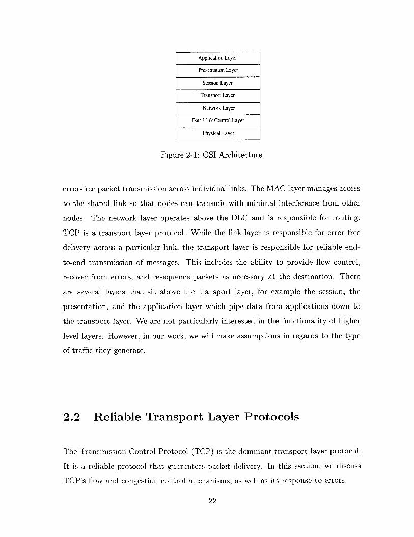
2-1 OSI Architecture . . . . . . . . . . . . . . . . . . . . . . . . . . . . . 22
3-1 Queue Management . . . . . . . . . . . . . . . . . . . . . . . . . . . . 38
3-2 Performance of 10KB and 100KB files as the load comprised by 10KB
files increases. . . . . . . . . . . . . . . . . . . . . . . . . . . . . . . . 60
3-3 Performance of 1MB and 10MB files as the load comprised by 1MB
files increases. . . . . . . . . . . . . . . . . . . . . . . . . . . . . . . . 61
3-4 The Performance of Short Files as Length Increases . . . . . . . . . . 63
4-1 The Effect of the Mean Backoff Time on System Goodput . . . . . . 84
4-2 The Effect of the Advertised Window Size on System Goodput . . . . 86
4-3 The Effect of MAC Layer Retransmissions on System Goodput . . . 87
4-4 Simulation and Theoretical plots of System Goodput vs Load . . . . 89
4-5 The Affect of the Number of Sessions on Goodput . . . . . . . . . . . 90
4-6 Round Trip Time and Variance . . . . . . . . . . . . . . . . . . . . . 93
4-7 Probability of Collision . . . . . . . . . . . . . . . . . . . . . . . . . . 95
4-8 TCP Collision Discovery . . . . . . . . . . . . . . . . . . . . . . . . . 97
4-9 Wasted Transmissions . . . . . . . . . . . . . . . . . . . . . . . . . . 98
4-10 Comparing the Offered Load to the System Goodput . . . . . . . . . 100
11

12

List of Tables
1.1 Summary of Current Satellite Systems [30] . . . . . . . . . . . . . . . 17
3.1 Ten sessions. One session has a packet loss rate of 10%. . . . . . . . . 53
3.2 Ten sessions. Half of the sessions have a packet loss rate of 10%. . . . 53
3.3 Ten sessions. One session has packet loss rate of 1%. . . . . . . . . . 53
3.4 Ten sessions. Half of the sessions have a packet loss rate of 1%. . . . 54
3.5 Ten sessions. One Session has a RTT of 1.0s, and the others have a
RT T of 0.5s. . . . . . . . . . . . . . . . . . . . . . . . . . . . . . . . . 56
3.6 Ten sessions. Half of the sessions have a RTT of 1.0s, and the others
have a RTT of 0.5s. . . . . . . . . . . . . . . . . . . . . . . . . . . . . 56
3.7 Ten Sessions. One session has an RTT of 0.01s, and the others have a
RT T of 0.5s. . . . . . . . . . . . . . . . . . . . . . . . . . . . . . . . . 56
3.8 Ten Sessions. One session has an RTT of 0.01s, and the others have a
RT T of 0.01s. . . . . . . . . . . . . . . . . . . . . . . . . . . . . . . . 56
3.9 Ten Sessions. Five Sessions have RTTs of 0.01s, and the others have a
RT T of 0.5s. . . . . . . . . . . . . . . . . . . . . . . . . . . . . . . . . 56
13

14
Chapter 1
Introduction
1.1 Satellite Communications
Current satellite communications systems mainly serve a niche market. Their ser-
vices are used by the military for surveillance and for on-the-ground communications.
Satellite services are also used by individuals living in areas without cellular cover-
age or proper telecommunications infrastructure. Satellites are useful in connecting
geographically distant locations as well.
1.1.1 Introduction
History of Satellite Networks
Satellite communications systems have been in use for a considerable amount of time.
AT&T launched the first communications satellite into orbit in 1962. Since then,
countless other communications satellites have been sent into orbit. Originally, they
had a fixed purpose in the communications framework; they served as transoceanic
links and were used by television stations to broadcast audio and video. In the 1990's,
satellite service was further extended with DBS (Direct Broadcast Satellite). Today,
end users are able to receive audio and video directly through satellites. There are
well over 1,000 communications satellites currently in orbit.
Satellite systems offer many advantages over terrestrial telecommunications sys-
15

tems. They include [9]:
" Ubiquitous Coverage A single satellite network can reach users worldwide.
They are capable of reaching the most remote and unpopulated areas. Terres-
trial communications networks require a considerable amount of infrastructure
to function. Therefore, it is often not cost effective to place them in sparsely
populated or remote areas.
" Rapid Deployment As soon as a satellite network is launched, it has global
reach and can serve the whole world. For terrestrial based networks to ex-
tend their reach, base stations and switching stations need to be build locally,
a non-expensive procedure. The local infrastructure must then be connected
to a main communications hub, so that it can have global reach. In addition,
existing satellite systems could be extended to support areas that lack telecom-
munications infrastructure. In which case, it may not be necessary to even build
infrastructure for terrestrial communications networks.
" Reliability Once a satellite is in orbit, it very rarely fails. In fact, satellite
networks are one of the most reliable types of communications networks, behind
optical SONET systems.
Current Satellite Systems
In the late 80's and early 90's, several satellite systems were launched with consider-
able hype and fanfare. The systems appeared promising in part because they were
sponsored by prominent individuals and companies, including Motorola, Bill Gates,
Qualcomm, etc. These systems included Iridium, Globalstar, Teledesic, INMARSAT,
and others. However, satellite systems failed to attract the number of customers an-
alysts predicted, costs were too high and the equipment was too bulky. Following
Iridium's bankruptcy filing and the failure of Teledesic, the satellite telecommunica-
tions industry was considered dead. Before filing for bankruptcy, Iridium was charging
$7/min for phone calls with handsets costing $3,000 a piece. More recently, Iridium
has mounted a come back. Iridium was awarded a large Department of Defense con-
tract and has since shored up its system. In the span of three years, the cost of
16

Name Iridium INMARSAT GlobalStar Teledesic Direct TV
Owner originally Comsat Loral and Bill Gates and Hughes
Motorola Qualcomm Craig McCaw
# of satellites 66 6-20 48 (only 40 used) none in orbit 7
Services voice and data voice and data voice and data data at 2Mbps digital TV
at 2.4Kbps at 2.4Kbps at 9.6Kbps
Started Service 1998 1993 1997 2002 1994
Table 1.1: Summary of Current Satellite Systems [30]
handsets has been cut in half and the cost of a phone call is down to $1.50/min.
These costs are expected to continue decreasing. Currently, the US and the British
military are among Iridium's largest clients. Analysts project that in an environment
of heightened security, satellite communications systems, which are difficult to sabo-
tage, have the potential to tap into an as of yet untouched market [31, 27]. Although
Iridium has met with success in the military field, it has had limited success with
consumers, in part owing to high prices. Globalstar is a satellite data and voice com-
munications system that has done quite well commercially. Like Iridium, Globalstar
suffered through bankruptcy filings, but is now relatively stable. Globalstar customers
typically live in areas with poor cellular coverage that include rural areas. Additional
customers travel or work in remote areas at sea or in the desert. Per minute charges
for Globalstar are substantially lower than those of Iridium, and can be as low as
$0.25. However, Globalstar does not have the complete global coverage of Iridium
[38]. Another popular satellite based system is Direct TV. It is owned by Hughes and
has well over 12 million customers world wide. There are several other popular satel-
lite services available, including DishNetwork, which boasts several million customers
as well.
1.1.2 Integration of Satellites and the Internet
The market for broadband satellite services is expected to reach $27 billion by 2008,
and it is anticipated that there will be 8.2 million subscribers of broadband satellite
services [9]. See Figure 1-1. With the cost of building, launching, and maintaining
satellites falling and the demand for bandwidth and telecommunications related ser-
17

vices increasing, satellite systems are a viable way to increase capacity for Internet
based services. Broadband satellite networks will be able to bring high speed Inter-
net into more homes and bring the Internet to people who have never used it before.
Satellite services are also capable of introducing the Internet to developing countries
with limited telecommunications infrastructure.
4000
3500
3000
E2500
2000C
S1500zU
1000
500
Satellite Access to the Intemet
1999 2000 2001 2002 2003 2004year
2005 2006 2007 2008
Figure 1-1: Market for Broadband Satellite Services [3]
In addition to Direct TV, Hughes also owns the fairly successful DirectPC which
provides high speed Internet access to its users. It is especially popular in areas where
high speed DSL and cable are not available. Direct PC users enjoy data rates almost
ten times greater than those provided by dial-up modems. However, they are still
not as fast as terrestrial based cable and DSL systems. Despite the fact that rates
are not quite as high as DSL yet, satellite based services are the only means of high
speed data connections possible for people in rural areas.
1.2 Contributions of the Thesis
In this thesis, we discuss two separate problems. Both topics, however, relate to the
interaction of the Transmission Control Protocol (TCP) with other network protocols.
18

1.2.1 Problem Statement
We are interested in learning how TCP interacts with protocols at the Medium Access
Control (MAC) Layer.
" Scheduling at Bottleneck Links
We want to design queue management policies that are capable of providing
increased performance at bottleneck links. We are not exclusively interested
in enhancing the overall goodput of the network. We are also interested in
ensuring that sessions traveling across lossy channels get their fair share of
network resources. In addition, we explore the effects of persistent traffic on
short file/message transfers.
" Combining TCP with Random Access Protocol
Little headway has been made in studying the interaction between transport
and random access MAC layer protocols. We attempt to gain intuition behind
the joint behavior of TCP and the ALOHA class of protocols through simula-
tion. We focus on the maximization of goodput, as well as delay and collision
discovery.
1.2.2 Contributions of the Thesis
We designed two new queue management schemes that are capable of providing high
levels of fairness to isolated sessions transmitting across lossy links. In addition, our
scheduler transmits short messages with priority to reduce the latency they experi-
ence. We call our queue management policies Shortest Window First and Smallest
Sequence Number First with Approximated Longest Queue Drop (SWF with ALQD
and SSF with ALQD, respectively). Our queue management schemes are unique in
that they employ metrics for scheduling and packet admission that have never been
used before. Specifically, our metrics come from the packet header. SSF and SWF
use the TCP sequence number and the TCP congestion window size, respectively, to
prioritize packets.
19

In addition to the scheduling problem, we provide insight into the interaction of
TCP and ALOHA. Through simulation, we isolate TCP and ALOHA parameters
and then optimize them for maximum throughput. We also focus on how the retrans-
mission policies of TCP and ALOHA interact with each other. Results indicate that
ALOHA can use its retransmission abilities to hide collisions from TCP, thus reducing
the frequency with which TCP's congestion control apparatus must be invoked. By
far, our most interesting result shows that running TCP aver ALOHA can stabilize
ALOHA's performance.
1.2.3 Thesis Overview
Chapter 2 provides an overview of network architecture. We spend considerable time
on the functioning of the Transmission Control Protocol. In addition, we discuss
general classes of MAC layer protocols that can be implemented. Chapter 3 is devoted
to the study of the behavior of the Transmission Control Protocol when a fixed
access Medium Access Control Protocol is used. Section 3.1 discusses several current
active queue management schemes. In the following sections, we discuss our own
schedulers and their performance in a variety of different environments. In Chapter
4, we consider the dynamics involved in integrating the Transmission Control Protocol
with a random access Medium Access Control Protocol. In section 4.2, we discuss a
variety of random access protocol. Section 4.4 highlights some of the interactions we
expect to observe between the transport and medium access control layers. The later
sections serve to verify our hypotheses through extensive simulation. We conclude
and summarize our results in Chapter 5.
20

Chapter 2
Background and Model
Construction
In this chapter we introduce the OSI Model and discuss the two network layers that
are relevant to our work: the transport layer and the MAC layer. The Transmission
Control Protocol (TCP) is the transport layer protocol that we consider. We discuss
TCP and its performance in space networks. We also consider a couple of MAC layer
protocols as well, and conclude with a discussion of our models.
2.1 Network Model
TCP does not operate in isolation. It is coupled with other protocols, most often
IP (the Internet Protocol), hence the famous TCP/IP protocol suite. However, TCP
can operate with other protocols as well. In order to understand TCP's performance
in the network, it is necessary to understand its relation to other network protocols.
Under the Open Systems Interconnection (OSI) architecture, networks are divided
into seven layers. See Figure 2-1. Each layer is associated with a particular set of
functionalities. The physical layer is the lowest layer and is responsible for the actual
transmission of bits over a link. It is essentially a bit pipe. The data link control layer
(DLC) is the next higher layer. It is often treated as two sub-layers, the logical link
layer (LLL) and the medium access control (MAC) layer. The LLL is responsible for
21
Application Layer
Presentation Layer
Session Layer
Transport Layer
Network Layer
Data Link Control Layer
Physical Layer
Figure 2-1: OSI Architecture
error-free packet transmission across individual links. The MAC layer manages access
to the shared link so that nodes can transmit with minimal interference from other
nodes. The network layer operates above the DLC and is responsible for routing.
TCP is a transport layer protocol. While the link layer is responsible for error free
delivery across a particular link, the transport layer is responsible for reliable end-
to-end transmission of messages. This includes the ability to provide flow control,
recover from errors, and resequence packets as necessary at the destination. There
are several layers that sit above the transport layer, for example the session, the
presentation, and the application layer which pipe data from applications down to
the transport layer. We are not particularly interested in the functionality of higher
level layers. However, in our work, we will make assumptions in regards to the type
of traffic they generate.
2.2 Reliable Transport Layer Protocols
The Transmission Control Protocol (TCP) is the dominant transport layer protocol.
It is a reliable protocol that guarantees packet delivery. In this section, we discuss
TCP's flow and congestion control mechanisms, as well as its response to errors.
22

2.2.1 The Transmission Control Protocol
In our discussion of TCP, we focus on a particular variant, TCP Reno. TCP Reno
is one of the most widely used versions of TCP, and it is also one of the most widely
studied protocols. Using TCP Reno in our analysis and simulations allows us to make
better comparisons between our work and that of others.
TCP provides a reliable, in-order, end-to-end byte-streaming data service [32]. It
is a connection-oriented service that is capable of providing both flow control as well
as congestion control. The TCP sender accepts data from higher-level applications,
packages it, and then transmits it. The receiver, in turn, sends an acknowledgment
(ACK) to the transmitter upon receipt of a packet.
Basic TCP
The TCP protocol is based on a sliding window. At any given point, TCP is only
allowed to have W outstanding packets, where W is the window size. The window
size is negotiated between the sender and receiver. The sender then sets its window
size to a value less than the advertised size, preventing it from overwhelming the
buffer of the receiver. Thus, flow control is achieved.
When the destination receives an in order packet, it slides its window over and
returns an ACK to the sender. When the sender receives an acknowledgment, it
slides its window to the right. However, if the sender does not receive an ACK for a
packet it sent within a certain timeout (TO) interval, it retransmits the packet and
all subsequent packets in the window. We refer to this as a retransmission timeout
(RTO) event. Clearly, setting the timeout interval correctly is critical. If it is too
short, spurious retransmissions are sent, and if it is too long, sources wait needlessly
long for ACKs. Typically, the timeout interval is computed as a function of the round
trip time (RTT) between the sender and receiver. For more details, see Appendix A.
Congestion control is different from flow control. In flow control, the receiver
attempts to prevent the sender from overflowing the receiver buffer. Congestion
control is a resource management policy within the network that attempts to avoid
congestion. In addition to the general window, TCP also has a congestion window for
23
each connection. This provides an additional constraint. Now, the maximum number
of unacknowledged packets allowed is the minimum of the congestion window and the
advertised window size.
TCP determines the size of the congestion window based on the congestion it
perceives in the network. As the congestion level increases, the congestion window
decreases, similarly when the congestion level decreases, the congestion window in-
creases. TCP assumes that all losses are due to congestion. Therefore, when a packet
is lost, the congestion window is halved. Every time a congestion window worth of
packets has been successfully received and ACKed, the sender's congestion window
is incremented by a packet. (Alternatively for every ACK received, the congestion
window is incremented by 1/W.) Taken together, this is known as the additive
increase/multiplicative decrease policy [2]. The additive increase/multiplicative de-
crease policy is necessary for the stability of the congestion control policy. It is
important to increase the congestion window conservatively. If the congestion win-
dow is too large, packets will be dropped, and retransmission will be required, further
increasing the congestion level of the network.
TCP Extensions
Although the additive increase/multiplicative decrease policy works, it takes a con-
siderable amount of time for the congestion window to reach a size at which it is
fully utilizing network resources. This is especially true in the case of broadband net-
works. Current TCP protocols no longer use the pure additive increase/multiplicative
decrease algorithm defined above. Instead, they use slow start and congestion avoid-
ance.
The slow start algorithm was developed to ameliorate the situation [36]. Slow
start decreases the time it takes to open up the congestion window. Under slow start,
for every acknowledgment received, the sender's congestion window is increased by
one packet. The size of the congestion window doubles every RTT. Slow start is used
initially to rapidly open up a connection. It is also used if a sender has timed out
while waiting for ACK, in which case the congestion window is set to 1. Slow start
continues until the congestion window reaches the slow start threshold, which is half
24
the value of the congestion window size at the time the last loss event was detected.
At this point, TCP exits slow start and enters the congestion avoidance phase. In
congestion avoidance, the window is opened much more conservatively, to avoid a
loss event. The last loss event occurred when the congestion window size was Wprev.
The TCP sender remembers that the last time congestion was experienced at the
window size of Wpev. Therefore, when the window size reaches Wpr,,e/2, it changes
its window increase policy from slow start to congestion avoidance. It slows down
the growth of the congestion window to decrease the speed with which it reaches a
window size that causes congestion. In congestion avoidance, the congestion window
typically increases by one packet every RTT.
Waiting for TCP timeouts can lead to long periods where the channel is idle, no
data is transmitted and as a result bandwidth is wasted. The fast retransmit strategy
was developed to avoid long periods of idle. Fast retransmit triggers a retransmission
before a timeout event occurs. TCP with fast retransmit is altered, so that the
receiver sends an ACK for every packet it receives. If it receives an out of order
packet, it will simply acknowledge the last in order packet it received. Therefore, it is
possible for the sender to receive duplicate ACKs. Receiving one duplicate ACK is not
sufficient to assume that a loss has occurred. However, if multiple duplicate ACKs
are received, it is a strong indication that the packet following the acknowledged
packet has been lost and needs to be retransmitted. In the current fast retransmit
standard, if the sender receives three duplicate ACKs, it will retransmit the packet.
A trade-off is made in fast retransmit between retransmitting packets spuriously and
waiting for a timeout to indicate a loss. In TCP Reno, fast retransmit is paired with
fast recovery. Fast recovery avoids using slow start after fast retransmit. Instead, it
simply cuts the congestion window in half and begins retransmission in congestion
avoidance under additive increase. See Appendix A for more information on TCP
Reno's fast retransmit and recovery mechanisms.
The receipt of duplicate acknowledgments suggests that the loss event was due to
transmission errors and not congestion. After all, if congestion was the cause of the
loss, we would not expect to receive any ACKs, and a timeout event would occur.
25

TCP Reno, therefore, does attempt to rudimentally distinguish between losses due to
congestion and losses due to transmission error. If the loss is detected by duplicate
ACKs, the congestion window is not reduced as drastically as it is when a timeout
event occurs. It has been argued that if losses are due to transmission error then con-
gestion control should not be invoked. However, TCP Reno is a conservative protocol
and duplicate ACKs do not definitively prove that the loss was due to transmission
error. Therefore, TCP Reno reduces the congestion window, albeit not as drastically
as it could.
2.3 TCP Performance Over Satellites
The performance of TCP over satellite links differs greatly from that in wired links.
We discuss the characteristics of satellite links and problems that can arise. We
conclude by discussing current research on TCP enhancements for higher performance
in satellite networks.
2.3.1 Characteristics of Satellite Links
TCP is known to perform well in terrestrial networks as witnessed by its overwhelm-
ing popularity in Internet applications. The performance of TCP is affected by band-
width, delay, and bit error rates. However, in satellite networks these parameters
often differ substantially from those seen in terrestrial wired networks. We discuss
these properties below.
e High Bandwidth: The high bandwidth offered by satellite networks is its most
desirable feature. Unfortunately, several other properties of satellite channels
prevent full utilization of available bandwidth.
e High Propagation Delay: The end-to-end latency experienced by users in-
cludes transmission delay, queuing delay, and propagation delay. In satellite
networks, the propagation delay is typically the largest component of the over-
all delay experienced. In geostationary (GEO) satellite networks, which we
26

consider in this thesis, round trip propagation delays (this includes both the
transmission of data and the receipt of an ACK) approach and even exceed
500ms. The bulk of the delay is associated with the uplink and downlink. How-
ever, links between satellite repeaters also add delay, typically on the order of a
few milliseconds per link. These high round trip delays have a huge impact on
the speed with which the TCP congestion window opens. Small file transfers
may experience unnecessarily long delays due to the fact that it will take several
RTTs before the congestion window has opened up to a sufficiently large size.
High Bit Error Rates: The bit error rates (BER) seen in satellite networks
are considerably higher than those seen in terrestrial networks. Bit error rates
in satellite networks can vary anywhere from 10-4 to 10-6. In addition, trans-
missions are also subject to effects that hamper wireless communications, like
fading and multipath. Since TCP assumes that all losses are due to congestion,
it will invoke its congestion control mechanism each time it experiences a loss.
In satellite networks, losses are frequently due to bit errors. The congestion
window's growth is impeded by perceived network congestion.
2.3.2 Problems with TCP over Satellite Links
Although, the performance of TCP has increased over the years, many problems still
remain. The deficiencies we mention below are not specific to satellite networks. They
also degrade performance in terrestrial wireless networks and to some extent wired
networks as well.
* Bandwidth Unfairness: TCP has been shown to provide unfair bandwidth
allocation when multiple sessions with differing RTTs share the same bottleneck
link. Sessions with large RTTs are unable to grow their windows as rapidly as
sessions with smaller RTTs. In fact, sessions with large RTTs maybe almost or
completely shut out by competing sessions with smaller RTTs, since short RTT
connections will obtain the available bandwidth before the long connections
even have a chance. The bias against sessions with long RTTs goes as RTT',
27

1 < a < 2 [24].
Efforts to improve the fairness of TCP have mostly focused on two different
areas, the development of active queue management (AQM) schemes as well as
actual modifications of TCP. AQMs like FRED and Fair Queuing have had some
success. However, AQMs only work if sessions have packets to send, therefore
their effectiveness is limited by TCP's window growth algorithm. Both FRED
and Fair Queuing will be discussed in more detail in Chapter 3. To achieve
real improvement in terms of fairness, changes are needed in TCP's congestion
control and window control mechanism. Attempts to combat RTT bias through
the use of a Constant-Rate (CR) policy are seen in [21]. In the CR policy, the
additive increase rate is c - RTT, which lets all sessions increase at the same
rate. The congestion window, cwnd, increase algorithm becomes
cwnd = cwnd + min((c - RTT - RTT) /cwnd, 1), (2.1)
where c controls the rate. This policy, which modifies the existing TCP stan-
dard, allows all sessions, regardless of their RTT, to additively increase their
congestion window at the same rate.
Handling Errors: TCP assumes that all losses are due to congestion. There-
fore, when a loss is detected, even if it is due to a transmission error, the TCP
congestion window will at a minimum be reduced by a factor of a half. A re-
duction in the congestion window size, however, is unnecessary, if the loss is
due to a transmission error. Over time, these losses can substantially decrease
throughput, as it will take the session many RTT times to grow its congestion
window to its former size.
TCP's performance would be greatly improved if it were able to discern trans-
mission error based losses from congestion oriented losses. There are several
ways one could attempt to do so, and solutions typically fall into one of three
classes: end-to-end, link layer, and split connection [5]. We discuss the split
28

connection approach later, therefore we focus on end-to-end and link layer ap-
proaches here. In end-to-end protocols, the TCP sender handles losses through
one of the two techniques, Selective Acknowledgments (SACKs) and Explicit
Loss Notification (ELN). SACKs inform the TCP sender if multiple sequential
gaps exist in the receive buffer - if multiple losses have occurred. The sender
then only has to retransmit the missing packets as opposed to the missing pack-
ets and all subsequent packets as TCP Reno may have to. It has been shown
that TCP SACK performs better than baseline TCP [23]. Using the ELN ap-
proach, if the receiver receives a packet with an error, it sets a bit in the ACK
header to notify the TCP sender that the loss was not due to congestion. The
sender then retransmits the packet, but without activating any of the congestion
control functions.
Link layer approaches attempt to hide losses from the TCP sender through
the use of local retransmissions. Retransmissions can be performed using any
standard automatic repeat request (ARQ) protocols. Both the performance of
stop and wait [7] and the more complicated Go Back N and Selective Repeat
[26] protocols have been examined.
* Slow Start: TCP uses slow start to rapidly open up its congestion window.
However, if the link bandwidth is very large, slow start's exponential growth may
not be aggressive enough. In addition, there is a concern that if a transmission
error occurs during slow start, the session will enter congestion avoidance too
soon. It will bypass the high growth phase offered by slow start. Thus, window
growth occurs very slowly leading to potential reductions in throughput.
Studies have suggested that increasing the initial window size of a TCP con-
nection can improve performance [1, 33]. However, this enhancement only has
a short term effect. It is not particularly helpful for long running connections.
Researchers have also investigated whether modifying the additive increase pol-
icy of congestion avoidance can increase throughput [21]. Instead of increasing
the window size by one packet every RTT, the window is increased by K pack-
29

ets every RTT. It has been determined, not surprisingly, that the throughput
of a connection increases with K. However, if only one session sharing the
bottleneck link is using the "increase by K" policy, large values of K can lead
to unfair bandwidth allocations. Perhaps the "increase by K" and CR policy
could be combined to limit unfairness and improve performance.
Heterogeneity: TCP is detrimentally effected by poorly performing links. In
fact, its performance is limited by the worst link in the network. For this reason,
performance in heterogeneous networks with both wired and wireless networks
is mediocre at best.
Many researchers have advocated creating split connections to combat this lack
of homogeneity [5, 4, 39]. The developers of Indirect TCP suggest splitting
TCP connections into two separate connections, one connection between the
wireless terminal and the mobile switching station and the other between the
mobile switching station and the wired network [4]. Using their architecture,
loss recovery can be handled independently in the wireless and the wired portion
of the connection. Furthermore, specialized versions of TCP can be run over
the wireless connection to improve performance. The key is to shield the source
in the wired network from the losses experienced in the wireless portion of the
network. One problem with this approach is that it violates the end-to-end
property of TCP acknowledgments. However, many variants of this approach
have been subsequently proposed.
2.3.3 TCP Enhancements for Satellite Links
Research on TCP for satellite networks has increased over the years. In this section,
we consider two different transport protocols for the space environment, the Satellite
Communications Protocol Standards - Transport Protocol (SCPS-TP), a modified
version of TCP, and the Satellite Transport Protocol (STP). Besides these two efforts,
there is also an ongoing consortium effort to find modifications to enhance TCP
performance over satellites [12].
30
SCPS-TP is an extension of TCP for satellite links [11]. Many of the modifi-
cations it recommends for TCP have been applied to terrestrial wireless networks
as well. SCPS-TP distinguishes between losses due to congestion, link outages, and
random transmission errors. Instead of assuming all losses are due to congestion,
SCPS-TP has a parameter controlled by the network manager that sets the default
cause of packet loss. SCPS-TP also makes use of ELN techniques; acknowledgments
specify the reason of the loss. Therefore, if a loss is determined to be due to trans-
mission error, congestion control will not be invoked. SCPS-TP also has the ability
to deal with link asymmetries on the reverse channel. Delayed ACKs are used to
limit the traffic on the reverse channel. The only problem is this essentially disables
the fast retransmit algorithm of TCP. SCPS-TP also uses Selective Negative Ac-
knowledgments (SNACKs) to reduce traffic on the reverse channel and provide more
information. The receiver only sends an acknowledgment if it finds that there are
gaps in the sequence of received packets. The SNACK is a combination of a SACK
and a NAK. It can specify multiple gaps in the sequence of received packets.
STP is a transport protocol that is optimized for high latency, bandwidth and path
asymmetries, and high bit error rate channels [20, 22]. It bears many similarities to
TCP, but it is in fact meant to replace TCP. In this sense, it is different from SCPS-
TP which for all extents and purposes is simply a modified version of TCP. Still,
STP bears several strong resemblances to SCPS-TP. Like SCPS-TP, STP also uses
SNACKs. This disables the fast retransmission mechanism of TCP. However, STP
further dismantles TCP's congestion control mechanism by not using any retransmis-
sion timers. Without retransmission timers, timeouts cannot occur. Furthermore,
slow start will only be entered once, at the very beginning of a connection; the STP
source will never reenter slow start. TCP uses ACKs to trigger its congestion window
increase mechanism, and thus also uses them to trigger transmissions. STP, in effect,
has extremely delayed ACKs. The receiver will send out SNACKs when it notices a
gap in the receive buffer, and the sender will periodically request SNACKs to learn
the status of the receive buffer. STP's congestion control mechanism is triggered by
the receipt of these SNACKs.
31

STP offers somewhat higher throughput than TCP and its variants. However, its
strongest point is the reduction in required reverse channel bandwidth. The devel-
opers of STP envision its use in two different scenarios: as the transport protocol of
the satellite portion of a split connection or as the transport protocol for the entire
network. Unfortunately, despite the benefits it offers, STP has not really taken off.
We suspect this is due to the fact that it makes such a large departure from TCP.
2.4 MAC Layer Protocols
In this thesis, we exclusively use TCP as our transport layer protocol. However, we
examine different MAC layer protocols. MAC layer protocols control the way in which
sessions are able to access a shared channel for transmission. They are responsible for
scheduling the transmission times of sessions to avoid interference whenever possible.
MAC layer protocols fall into two different categories: fixed access and random access.
Fixed Access Protocols
Fixed Access protocols include multiple access technologies like Frequency and Time
Division Multiple Access (FDMA and TDMA, respectively). Another commonly
used multiple access strategy is Code Division Multiple Access (CDMA), which can
be thought of as a hybrid of FDMA and TDMA. FDMA and TDMA are the easiest
fixed access protocols to describe; we focus on them here. These access schemes are
perfectly scheduled. The shared channel is divided into slots, based on either time or
frequency. If FDMA is used, each session is allocated a frequency slot for its exclusive
use. In TDMA, each session is allocated a certain time slot during which it can
transmit. In their slot, sessions have exclusive use of the entire channel bandwidth.
Slot allocation in TDMA typically occurs in round robin fashion. One of the potential
drawbacks of fixed access protocols is their centralized nature. Synchronization is
needed between all users, so that they transmit in their correct slots without overlap.
This is especially important for TDMA systems. If the system is lightly loaded, either
the data rate of the system is low or the number of active users is small, the latency
experienced by users may be unnecessarily high. Users will have to wait several empty
32

slots before it is their turn to transmit.
Random Access Protocols
Random access protocols include technologies like ALOHA and Carrier Sense Multiple
Access (CSMA). In this family of protocols, users transmit packets as soon as they
receive them (the simplest case). Transmitters hope that no other session attempts
to transmit at the same time. If multiple sessions transmit at the same time, a
collision occurs, and the colliding packets will require retransmission. Random access
schemes are well suited to lightly loaded networks. Sessions experience low latencies
in comparison to fixed access systems and collisions are rare. Random access schemes
are fully distributed and flexible in terms of the number of users they can support.
However, as the number of sessions sharing the channel increases, the throughput of
multiple access systems is likely to decrease, due to the increase in the probability of
collision. We will return to this topic in much more detail in Chapter 4.
2.4.1 Model Construction
The model we consider in motivating our study is quite straightforward. Instead of
accessing the Internet through traditional local area networks (LANs) like ethernet
or broadband cable, we transmit data across satellite backbones.
The Centralized Model
In the centralized model, we consider persistent high data rate connections that share
the same bottleneck link. We assume that sessions are able to reach the bottleneck
link/satellite gateway through the use of a fixed access protocol. In this case, we
do not worry about collisions. We are concerned with the behavior of the satellite
gateway. How does it allow packets into the satellite network? How does it schedule
packets for transmission?
As a motivating example, consider the case of several large corporations that
constantly transmit and receive data. They connect to the Internet via a satellite
gateway. These sessions are always "on", and the system is typically heavily loaded.
The Internet Service Provider (ISP) which owns or leases the satellite knows in ad-
vance how many sessions it needs to provision for. With an accurate estimate of
33

the number of active sessions and a heavily loaded network, fixed access protocols
are used. Potential bottlenecks could arise at the gateway to the satellite network.
We want to assign packet transmission times at congested links that ensure all users,
regardless of their loss rate or RTT, get an equal share of the bandwidth and no
sessions face a latency penalty.
Another case of interest is when multiple users are transmitting across a shared
link, but they are transmitting messages of various sizes. Is it fair to treat long and
short sessions in the same way? If transmission start times are not simultaneous then
long sessions might be able to block the transmission of short sessions. We consider
this possibility in Section 3.3.
The Distributed Model
In the distributed model, we consider a sparse set of users that transmit sporadically.
As a motivating example, consider users of Iridium's satellite phones. They are
designed to be used from remote locations. In most cases, they are not used on a
regular basis, only in the case of emergency. The overall system load is relatively light
and the number of active sessions at any given time is unknown. Therefore, a random
access scheme is appropriate. In fact, the ALOHA protocol was originally designed to
facilitate communication between computer terminals and the central server for the
campuses at the University of Hawaii. We further generalize this scenario to the case
where multiple residential users rely on a satellite backbone for their Internet use.
With a variable number of users active at any given time, fixed access schemes are
difficult to implement efficiently. Therefore, random access schemes can be a viable
option. With the assumption of a lightly loaded system, bottleneck links are less of
a concern. The focus is on how sessions actually access the satellite router. How
do we optimize the performance of random access protocols under TCP for space
communications? We address this problem in Chapter 4.
34

2.5 Summary
In this chapter, we present today's ubiquitous transport layer protocol, TCP. Despite
its popularity, TCP has certain peculiarities which reduce its performance in satel-
lite networks. We detail the problems with TCP, and the solutions that have been
proposed. Unfortunately, none of these proposals provide a complete solution. We
also introduce MAC Layer protocols, both fixed and random access. We conclude by
describing the models we use in our simulations and provide the motivation behind
them.
35

36

Chapter 3
Scheduling at Satellite Bottleneck
Links
3.1 Introduction
We are interested in finding ways to increase both throughput and fairness through
the use of proper queue management at the link layer. Queue management is respon-
sible for allocating bandwidth, bounding delays, and controlling access to the buffer.
We view queue management as being composed of two independent components: the
scheduler and the packet admission strategy. See Figure 3-1. The scheduler is re-
sponsible for selecting packets from the queue and passing them to the physical layer
for transmission. In addition, it allocates bandwidth and controls the latencies expe-
rienced by users. In selecting packets for transmission, it determines which sessions
gain access to the channel. Total latency is comprised of the propagation delay, the
transmission delay, and the queuing delay. For the most part, the propagation and
the transmission delay characteristics are fixed for a given static network. However,
the queuing delay can be variable, depending on how the scheduler selects packets
for transmission. The other aspect of queue management is the packet admission
mechanism. The packet admission mechanism manages packet entry into the buffer.
Our discussion in this chapter centers around the case where multiple connections
are routed over the same satellite link. Packets from the different connections are
37

Scheduler
Packet DroppingPolicy
0 transit
Physical Layer
Figure 3-1: Queue Management
buffered at the satellite router. We develop a queue management policy for bottleneck
gateways that is capable of providing fair bandwidth allocation and lower latencies.
We discuss the various aspects of queue management. We then discuss our queue
management strategy and related heuristics.
3.1.1 Scheduling
Schedulers at the link layer are responsible for releasing packets to the physical layer
for transmission. They select the order in which the physical layer transmits packets.
The simplest scheduler is the First In First Out (FIFO) Scheduler. It sends packets
to the physical layer for transmission in the order that it receives them. The FIFO
scheduler does not exert any control at all over the allocation of bandwidth or latency,
since no real scheduling occurs. In gateways where FIFO scheduling is used, sources
have control over the allocation of the bandwidth and the delay. Typically, it is
the greediest source, the source with the lowest RTT and the highest data rate,
that controls these variables. FIFO serves connections in proportion to the share of
the buffer they occupy. Connections with low RTTs will send packets to the buffer
more rapidly and thus gain more service. This allows them to grow their windows
38

more rapidly, which in turn allows them to further increase their share of the buffer.
Therefore, when trying to guarantee fairness in terms of bandwidth allocation or
latency in a heterogeneous network, FIFO gateways are not very useful, unless they
are paired with good packet admission policies.
Priority Queuing is another form of scheduling and can be treated as a variation of
FIFO. The majority of packets are serviced in a FIFO manner. High priority packets
simply get to cut to the front of the queue. In priority queuing, certain packets take
precedence over others. Priority can depend on the source or the destination of a
packet, the packet size, or the type of data being transmitted. Within the broad
family of priority queuing, there are two types, preemptive and non-preemptive. In
preemptive priority queuing, high priority packets are transmitted immediately. If
a lower priority packet is being transmitted, it is interrupted and completed after
transmission of the high priority packet has concluded. In non-preemptive priority
queuing, high priority packets are serviced immediately after the packet currently
being serviced has completed transmission. Thus, in non-preemptive priority queuing
there is some queuing delay associated with the latency of high priority packets. The
problem with priority queuing, especially preemptive priority queuing, is that they
"starve" low priority traffic. High priority traffic can overwhelm the scheduler and
prevent low priority traffic from ever being served.
In Fair Queuing (FQ), schedulers attempt to guarantee each session an equal
or fair share of a bottleneck link. In the simplest version of FQ, routers maintain
separate queues for every active session. These individual queues are serviced in a
round robin fashion. When a flow sends a packet too quickly, its allocated buffer space
will be filled up. This prevents sessions from increasing their share of bandwidth at
the expense of less aggressive flows. Fair queuing schedules packets for transmission
to allow equitable distribution of bandwidth. However, there are some problems that
can arise in this naive round robin mechanism. If some sessions have larger packets
they will be able to gain more bandwidth than they are due. Therefore, what we
desire is a bit by bit round robin scheme, where sessions are served one bit at a time.
Unfortunately, this is not a realistic solution. Another variation of FQ is Weighted
39
Fair Queuing (WFQ). A weight is assigned to each flow. This weight specifies the
number of bits or packets that can be transmitted at each turn. Weights can be used
to allocate bandwidth to sessions with different packet sizes fairly. With weights, naive
round robin can be performed. Unfortunately, selecting weights when packet sizes are
not known a priori is not easy. Still, weights can also be used to treat certain classes
of traffic preferentially. Thus, WFQ can behave like priority queuing. Implementing
true FQ schemes are quite expensive at O(log(n)), where n is the number of active
flows [10].
Deficit Round Robin is a more efficient version, 0(1), of generic fair queuing
schemes. In deficit round robin, schedulers which we study in this thesis, the buffer is
sub-divided into buckets. When a packet arrives, it is hashed into a bucket based on
its source address. These buckets are then serviced in a round robin fashion. We are
particularly interested in deficit round robin schedulers where each bucket is allocated
a "quanta", n bits, of transmission at each turn [34]. If a bucket has quanta equal to
a packet, it can transmit a packet. Otherwise, it accumulates more quanta and waits
for its next turn. This solves the problem of variable packet size.
3.1.2 Packet Admission Strategies
Packet admission schemes are vital in the overall fairness of queue management
schemes. They control entry into buffers. The simplest packet entry policy admits
packets into the buffer until the buffer is full. Incoming packets that encounter a
fully occupied buffer are dropped, denied entry into the buffer. This packet dropping
mechanism is known as DropTail. DropTail packet dropping schemes heavily penalize
certain kinds of connections. For example, if multiple sessions are sharing the same
link, sessions with lower data rates or higher round trip times, experience a sub-
stantially greater number of packet drops in comparison to their competing sessions
[16].
Random Early Detection (RED) is another admission policy that was designed
to reduce congestion within networks [17]. It performs especially well with transport
layer protocols like TCP. RED is specified by a minimum threshold, Qm , a maximum
40

threshold, Qna, and a drop probability, p. RED computes a moving average of the
buffer size. If the average number of packets in the queue is less than the minimum
threshold, newly arriving packets are not dropped. If the number of packets in the
queue is greater than the maximum threshold, newly arriving packets are dropped
with probability one. If the number of packets in the queue is between the maximum
and minimum thresholds, packets are dropped with probability p. RED also has ECN
(Explicit Congestion Notification) capability and can notify sessions of congestion by
setting a bit in the packet header.
RED keeps the average queue size at the router small. Thus, it allows the router
to support bursts of traffic without buffer overflow. The smaller Qmrn, the larger
the bursts that can be supported. There is no bias against bursty traffic - RED
treats all flows the same. It has also been shown that RED prevents sessions from
synchronizing and reducing their congestion windows simultaneously.
RED uses the same drop probability on all flows. This, in addition to the fact that
it only drops incoming packets, makes it easy to implement. Unfortunately, when a
mixture of different traffic shares the same link, the use of the same drop probability
for all sessions can lead to unfair bandwidth allocation. Flow Random Early Drop
(FRED) is a modified version of RED designed to have improved fairness properties
[25]. FRED has been shown to be as fair as RED when handling flows that behave
identically. However, it shows increased fairness in handling heterogeneous traffic
being transmitted over a bottleneck link.
FRED behaves like RED. It uses the parameters Qmin, the minimum number
of packets a flow is allowed to buffer, and Qmax, the maximum number of packets
a flow is allowed to buffer, but introduces the global variable avgcnt, the average
number of packets buffered per flow. Sessions that have fewer than avgcnt packets
buffered are favored, that is they have lower drop probabilities, over sessions that have
more than avgcnt packets buffered. In order to function correctly, FRED must store a
considerable amount of state information; it needs to track the number of packets each
active flow has buffered. By looking at the occupancy on a per flow basis, flows with
high RTTs will effectively get preferential treatment, increasing bandwidth fairness.
41

More recently, admission strategies have been developed to ensure that short ses-
sions gain their fair share of bandwidth. RED with In and Out (RIO) is employed
at the bottleneck queue. RIO uses different drop functions for different classes of
traffic. In this case, two classes of traffic are considered, packets from short sessions
and packets from long sessions [19]. Using RIO-PS (RIO with Preferential Treatment
for Short Connections), the drop probability of packets from short sessions is less
than that of long sessions. In implementation, the drop probability of short sessions
is based on the average number of short packets already buffered, Qshort, whereas
the drop probability of packets from long sessions is based on the average number of
packets (long and short) that have been buffered. Packets are marked as being from
a long or short connection by edge routers. Routers maintain counters for all active
flows, when the number of packets they have seen from a particular flow exceed the
threshold, NL, packets are tagged as belonging to a long connection. Using RIO with
preferential treatment for short connections provides short file (5KB) transfers with
an average response time that is substantially less than DropTail and RED.
BLUE is another recently developed packet admission strategy [14, 13]. Admission
policies like RED and FRED admit packets into the buffer based on the number of
packets sessions have buffered. In essence, these policies, FRED and RED, use the
length of a flow as an indicator of the congestion level. BLUE bases its decisions on
the number of packet losses and idle events a session has experienced. BLUE uses
a drop probability, p, for all packets entering the buffer. If the number of packets
being dropped due to buffer overflow increases, then the drop probability, p, will be
increased as well. However, if the queue empties out, or it is noticed that the link has
been idle for a considerable amount of time, the value of p will decrease. BLUE has
been shown to perform better than RED both in terms of packet loss rates and the
buffer size. In addition, BLUE has recently been extended to provide fairness among
multiple heterogeneous flows.
Another packet dropping policy is known as Longest Queue Drop (LQD). If a
packet arrives at a buffer that is fully occupied, the LQD admission strategy drops
a packet from the flow with the largest number of packets in the buffer. The newly
42

arriving packet is then enqued. LQD has the effect of discriminating against high flow
sessions to the advantage of less aggressive sessions. However, the implementation of
LQD does not come without a cost. The router must keep a list of queue lengths for
each session. Keeping a sorted list has a complexity of at least O(log(N)), where N
is the number of active flows.
In Dynamic Soft Partitioning with Random Drop (RND), backlogged connections
are placed into two groups, those with occupancy Qj greater than b and those with Qj
less than equal to b, where b = B/n. n is the number of sessions, and B is the total
available buffer space [37]. The tail packet of a session from the group of sessions
where Qj is greater than b is dropped. This amounts to an approximated version of
LQD.
3.1.3 Comparison of Queue Management Strategies
Fair bandwidth allocation does not necessarily mean fair bandwidth usage. Schedulers
can attempt to allocate bandwidth equally among different sessions. However, if a
session has no packets to send because of a poor packet admission strategy, the
scheduler's purpose if defeated. In fact, the packet dropping mechanism can have more
of an impact on fairness than the scheduler [37]. In a study by Suter et al. [37], the
behavior of gateways using FIFO and FQ with a variety of different dropping policies
was compared. They compared RED and DropTail to LQD as well as approximations
of LQD like ALQD and RND. Interestingly, in their paper, they implement LQD and
its variants with packet drops from the front as opposed to the back because it triggers
TCP's fast retransmit and recovery process sooner. Thus, front drops can lead to an
increase in throughput. In general, per-flow admission policies, like LQD, ALQD,
and RND, all performed better than RED and DropTail.
43

3.2 Shortest Window First (SWF) and Smallest
Sequence Number First (SSF) Schedulers
When designing a scheduler, there are several potentially competing criteria to con-
sider, among them maximizing throughput and bandwidth fairness, while minimizing
the latency experienced by sessions. Often the idea of maximizing throughput can
conflict with the need to achieve bandwidth fairness.
TCP is known to treat high delay sessions unfairly. High delay sessions cannot
increase their windows as rapidly as low delay sessions. Thus, if multiple sessions
share a bottleneck link, high delay sessions are effectively blocked from gaining an
equal share of network resources. Designing a scheduler to combat unfairness in TCP
is possible. Fair queuing schemes were developed for this very reason. They allow all
sessions to obtain an equal share of bottleneck resources by transmitting in a round
robin fashion. However, it takes time for sessions to fully open their windows and
buffer packets at the bottleneck. It is at this point that fairness is achieved. The time
to receive an ACK is much greater than the time between successive transmission.
So in a round robin scheme, a slow session or a new connection will not have enough
packets buffered for transmission since an ACK has not been received to clock out
a new packet. High round trip time sessions will not have a packet to send at each
turn. Similarly, if users are engaged in relatively short-term transactions, the benefits
of fair queuing may not be realized. Windows might not be large enough. Opening
up the congestion window is key for us. We want to expedite the process so that
sessions will in fact have packets in the buffer awaiting transmission.
Our goal is to design a scheduler that can provide users with substantially lower
latencies over existing schedulers. This is not a question that is specific to satellite
networks; it could be applied to LANs as well. However, given that TCP window
growth is based on round trip delays, this problem is much more critical to satellite
systems where round trip delays are especially onerous. Thus in our formulation, we
consider satellite networks exclusively.
44

3.2.1 Shortest Window First Scheduler
In designing the SWF scheduler, we want packets from slow sessions, that arrive
less frequently, to be transmitted immediately. We define slow based on the session
window size; the smaller the source window size, the slower the session. Quantifying
whether or not a session is slow is difficult. We can only measure relative slowness
by comparing sessions sharing the same link. Sessions may have small windows for a
variety of reasons, the connection only just opened, the connection is lossy and suffers
from frequent time out and duplicate ACK events, or the connection has an especially
high round trip time. By scheduling packets based on window size, we are sensitive
to sessions that suffer from timeout events. In addition, by giving priority to sessions
with small windows, we allow sessions to rapidly open their congestion windows,
which is especially important for short lived sessions. Finally, the SWF scheduler
allows slow sessions to transmit their packets without lengthy queuing delays further
decreasing the latency they experience.
We find that using window size, as an indicator of slowness is especially useful,
especially in light of studies that suggest TCP connections with large window sizes
are much more robust to packet loss than those with small window sizes [25]. By
transmitting packets from slow sessions first, sessions with small windows should not
experience retransmission related timeout events.
Policy
Our queue management strategy was devised to improve performance in terms of
both fairness and delay. Again, we find it useful to discuss our queue management
policy in two parts, scheduling and packet admission.
Our scheduling policy is called Shortest Window First (SWF). It resembles a
priority queuing scheme. The scheduling policy is exactly what the name suggests.
Packets in the queue are ordered based on their window size, with packets from
sessions with the smallest windows at the front of the queue. Thus, packets with the
smallest windows are served first. However, there is an important difference in that
our priority scheme adapts over time. Packets are sorted to the front of the queue
45
depending on the number of other packets in the queue at the time and their window
sizes. This aspect is important because it prevents the network manager from having
to constantly calibrate the system.
The notion of preemption alone is not enough. The buffer's packet drop policy
must be considered as well. The packet admission strategy we use is ALQD. If
incoming packets find the buffer full, the packet at the end of the queue is dropped to
make room for the newly arriving packet. Because the router's queue is fully sorted,
the packet that is dropped is the packet that comes from the source with the the
largest window size. It is likely that the source with the largest window size occupies
the largest share of the buffer, hence, the LQD-like policy. However, there are times
when our packet dropping scheme may not be a perfect LQD. Though unlikely, due
to timeout events, there could be stale packets left in the buffer. Stale packets may
be stamped with a larger window size than their source currently has. Therefore,
we consider our dropping policy to be an ALQD. In addition, from now on when we
refer to the SWF scheduler, unless otherwise specified, we will understand it to be
implemented with an ALQD dropping policy.
3.2.2 Smallest Sequence Number First
The design of the SSF queue management scheme is very similar to the design of the
SWF scheduler discussed in the previous section. The main difference between the
SWF and SSF scheduler is the metric that is used to sort packets and set priority.
In the case of SSF scheduling, we use packet sequence numbers to determine priority.
The sequence number can be used as an indicator of slowness. Sessions that transmit
packets across lossy or high delay links will have smaller sequence numbers. They
simply cannot transmit packets as fast or as successfully. As with SWF scheduling,
the SSF scheduler assists slow sessions by aggressively growing their TCP congestion
window. This is accomplished by sorting packets with small sequence numbers to the
front of the queue.
Policy
We again separate the discussion of our queue management policy into two parts: the
46

scheduler and the packet admission policy. As the name suggests, SSF sorts packets
based on their sequence number. Packets with small sequence numbers are given
priority. Small sequence numbers suggest that a connection has either just started,
so we should grow its congestion window rapidly, or that a connection has a high RTT
or traverses a lossy channel, in which case we want to give it priority in an attempt
to combat the inherent unfairness of TCP.
As we realized with the design of the SWF scheduler, priority queuing alone is
not sufficient for our purposes. It is vital to have a well designed packet admission
policy. We implement an approximated version of the LQD policy. In fact, the ALQD
policy implemented here is not quite as refined as the one administered by the SWF
scheduler. If an incoming packet encounters a full buffer, it is sorted into the queue,
and the packet at the end of the queue is dropped. In essence, the packet with the
highest sequence number is removed. However, it is possible for a packet to have a
high sequence number, but originate from a session that just experienced a timeout
event. Such a session would not be allowed to have very many unacknowledged
packets in the network. In other words, the sequence number does not correlate to
the number of packets in the buffer as well as window size does.
3.2.3 Implementation Issues
We must consider the number of operations necessary to implement our schemes. We
look at computational complexity in terms of the number of operations necessary to
buffer a packet. The complexity per packet of both our SWF and SSF schedulers is
O(log(n)), where n is the buffer size. This is simply the cost of inserting an item into
a sorted list of length n. If n gets too large, our sorting based schedulers may not be
efficient. However, DRR, which is the most efficient approximation of FQ schemes,
uses an LQD packet dropping policy that incurs a per packet complexity cost of
O(log(m)), where m is the number of active sessions. This is the cost of maintaining
a sorted list of the number of packets buffered by each session. So although our
scheme is not computational inexpensive, it is not substantially more expensive than
the DRR implementation we consider. Furthermore, both the SWF and the SSF
47

scheduler can be implemented in a much less complex manner. The shared queue can
be broken into a set of sub-queues. Each sub-queue can serve packets from sessions
with window sizes (or sequence numbers, in the case of SSF) of a certain range. Each
of these smaller queues can be sorted at a much lower cost. To maintain the same
functionality as SWF (or SSF), the sub-queues are served in order of the range of
window sizes (the sequence numbers) they contain (smallest to largest). The resulting
cost per packet of this new implementation would be O(log(n')), where n' is the length
of the sub-queue.
Although not necessarily apparent in our initial description of the SWF and the
SSF scheduler, they can accommodate sessions with different packet sizes with a
simple change. Sessions with smaller packet sizes require a larger window in order
to obtain the same throughput as a session with large packets. Similarly, sessions
with small packets will have larger sequence numbers for the same level of goodput
as sessions that transmit larger packets. This places sessions with small packets
at a distinct disadvantage since their packets will be sorted towards the end of the
queue. Therefore, in the case where packet sizes are not homogeneous, the packet
size-congestion window product is the sorting metric used for SWF. Thus, sorting
is performed based on the number of unacknowledged bytes a session is allowed to
have. Packets with a smaller packet size-congestion window product are sorted to the
front of the queue. For the SSF scheduler, the metric used is the packet size-sequence
number product. Sessions that have successfully transmitted fewer bytes of data will
be given priority.
Until now, we have discussed general implementation issues for our sorting based
schedulers. However, both the SWF and SSF schedulers have individual idiosyncrasies
that deserve mention. In order for the SWF scheduler to function correctly, a few
adjustments to the TCP header are necessary. Our scheduler relies on a stylized TCP
header. TCP headers have a field for the window size, however this field contains the
advertised window size of the receiver, for flow control purposes. We require a field
for the current window size of the transmitter. One possibility is to simply overwrite
the window size field in the header. The size of the advertised window is really only
48
needed when the connection is first initialized. The other possibility is to create a new
field within the header. It would increase header overhead by no more than a byte.
With either of these changes, the SWF scheduler will be able to function correctly.
There are details that we have ignored up until now when discussing SSF. The first
problem is wrap around. Sequence numbers for persistent sessions can get very large
and exceed the length alloted to them in the TCP header field, at which point, they
wrap around. In the real world, sequence numbers never start at zero as a security
precaution. If users opened their connection with a sequence number of zero, snoopers
would have an easy time stealing bandwidth. The solution to both of these problems
is one in the same. In our theoretical world, we can ignore wrap around effects and
packet sniffers and start all sequence numbers at zero. However, in the real world,
instead of having the scheduler look for the sequence number in the TCP header,
the scheduler itself should keep track of the number of packets it has seen from each
session. This in essence would provide the same information as the sequence number.
The scheduler can then use this information to schedule packets, giving priority to
packets from sessions that have not been as active, have lower sequence numbers.
The downside is that such an implementation requires the scheduler to keep state
information in proportion to the number of sessions it serves. However, other policies
discussed earlier, like FRED, require that state information be kept as well.
3.3 Experimental Results
We perform simulations using the Network Simulator, ns - 2. In our simulations,
we consider the performance of our scheduler with sessions using TCP Reno. We
consider a variety of different traffic patterns and durations. We are most interested
in understanding the behavior of our scheduler in terms of bandwidth fairness and
delay. In our simulations, we consider goodput. The difference between goodput
and throughput is small but significant. Throughput simply refers to the amount of
data that is transmitted across a channel. Goodput refers to the amount of ACKed
data that is transmitted across a channel. When studying TCP, goodput is almost
49

always used instead of throughput. TCP retransmits packets if it does not receive
an acknowledgment within a certain interval. Throughput values can be misleading
since they include packet retransmissions and ACKs which do not add to goodput.
3.3.1 Model
We consider several sources accessing the gateway to a satellite network. These
sources access the gateway using a point-to-point MAC like TDMA. The gateway is
responsible for releasing packets from these different sources into the satellite network
so that they can reach their destination. The order in which packets are allowed
to enter and exit the gateway has a large impact on goodput, fairness, and delay
characteristics of the system. We compare our SWF and SSF scheduler with ALQD
to DRR with LQD and FIFO with DropTail.
3.3.2 Fairness
We consider the performance of the SWF and the SSF scheduler when supporting
persistent connections. We do not assume sessions are homogeneous. Rather we
consider ten different sessions some of which are transmitted across a lossy or high
propagation delay channel. Each of the ten sessions attempts to transmit a file of
infinite length. At the end of a 2000 second interval, we compute the goodput of
each session. We are interested in both measures of fairness as well as overall link
utilization. If link utilization is low providing a high level of fairness is inconsequential.
Link utilization is simply the system goodput over the bottleneck bandwidth. We
compute the fairness metric using the following equation
f airness ( b) 2 (3.1)
where n refers to the number of sessions sharing the bottleneck link and bi refers to
the portion of the bandwidth allocated to the ith session [8]. The fairness metric can
range anywhere from 1/n to 1, with 1 representing maximum fairness, a completely
equal distribution of bandwidth.
50

Lossy Channels
With ten sessions, ideally, each session would obtain 10% of the bottleneck bandwidth.
Therefore, in our case, where the bottleneck link is 1Mbps, each session should obtain
100Kbps. Unfortunately, neither the SWF nor the SSF scheduler can guarantee a
completely equitable division of scare resources. However, our scheduler does perform
better than either FIFO or DRR in terms of splitting bandwidth equally regardless
of whether sessions are homogeneous or not. See Tables 3.1 and 3.3 for results when
one of the ten sessions has a packet loss rate of 10% and 1% respectively. (Our packet
size is 1000 bytes which implies the packet error rates correspond to bit error rates
of at least 10' and 10-6, respectively.)
Based solely on a link utilization, total goodput, metric, DRR and FIFO both
perform better than SWF. The SSF scheduler has a total goodput similar to DRR
and FIFO. However, the percentage difference in the link utilization between SWF
and both DRR and FIFO is quite small, only 2-3%. We are also interested in the
fairness aspects of the queue management scheme's performance. The fairness metric
indicates a preference for both SWF and SSF. However, it does not do justice to the
increase in goodput SWF and SSF provide lossy sessions. The difference between
the fairness metric for our schemes and DRR is small, only 1%. This is likely due to
the fact that the fairness metric looks over all sessions, and only one of the sessions,
the lossy session, does not gain its rightful share of bottleneck bandwidth. Looking
specifically at the lossy session, our algorithms more than double the goodput achieved
by the FIFO scheduler and increase the goodput achieved by DRR by over 16%.
The increased performance for lossy sessions comes with minimal decrease to overall
goodput.
The lossy session performs poorly when FIFO is used because of the DropTail
policy. Packets from lossy sessions simply cannot gain access to the buffer. Under
DropTail, lossless sessions will have more packets in the buffer. Thus, they will
increase their window size and continues to increase their share of the buffer to the
detriment of lossy sessions. DRR is relatively more fair to lossy sessions. If packets
from lossy sessions are awaiting transmission, they will be transmitted in round robin
51

fashion. Part of the reason DRR performs well is due to its use of the LQD policy.
Under this policy, lossy sessions will always have access to the buffer. If DRR was
combined with DropTail instead, packets from lossy sessions would be shut out of
the buffer. The same holds true, to some extent, for SWF and SSF which use an
approximate LQD policy. If SWF and SSF were combined with DropTail instead of
ALQD, their fairness properties would suffer.
The decrease in overall goodput when using the SWF scheduler is due to priority
given to lossy sessions at the expense of lossless sessions. Lossy sessions will virtually
always have smaller window sizes than lossless sessions and be transmitted with high
priority and minimal queuing delay. In the case of buffer overflows, lossless sessions
will be penalized, not lossy sessions. But regardless of the priority SWF provides,
lossy sessions will still suffer from window closures due to the loss rate. This limits
the number of packets lossy sessions can transmit successfully. By giving priority
to lossy sessions, SWF increases the queuing delay of lossless sessions. This in turn
increases the session's RTT and reduces their goodput. In fact, one of the reasons
FIFO with DropTail has the highest goodput is that it disregards the lossy session
and gives priority to the lossless sessions instead, which keep increasing their window
sizes and pushing data through the network. FIFO does not expend any effort in
transmitting packets from lossy sessions that are unable to effectively increase their
window size.
When the packet loss rate is 1%, the SWF scheduler actually favors the lossy
session over lossless sessions. This is not the case when the packet loss rate is 10%. At
high loss rates, packets are lost so frequently that the congestion window is constantly
closing. Even though SWF gives the lossy session priority and increases the rate at
which the congestion window grows, the high loss rate prevents a significant number of
packets from ever reaching the satellite gateway. TCP's congestion control mechanism
is constantly being invoked. There are simply not enough packets in transit from the
lossy session. However, when the loss rate is 1%, the congestion window of the TCP
sender is moderately large, but still comparatively small enough so that its packets
are consistently routed to the front of the queue, and there are packets to transmit.
52

Scheduler Total Goodput Goodput of Lossy Average Goodput of Fairness
(bps) Session (bps) Lossless Session (bps)SWF w/ ALQD 926216 31094 99458 0.9533
SSF w/ ALQD 947261 31331 101770 0.9526DRR w/ LQD 951041 26534 102723 0.9456
FIFO w/ DropTail 953099 13453 104405 0.9242
Table 3.1: Ten sessions. One session has a packet loss rate of 10%.
Scheduler Total Goodput Average Goodput of Average Goodput of Fairness(bps) Lossy Session (bps) Lossless Session (bps)
SWF w/ALQD 930050 29258 156750 0.6804SSF w/ALQD 940760 29219 158930 0.6779DRR w/LQD 949450 27262 162630 0.6630
FIFO w/DropTail 951340 12858 177410 0.5721
Table 3.2: Ten sessions. Half of the sessions have a packet loss rate of 10%.
As the number of poorly performing sessions increase, the performance of SWF
decreases. See Tables 3.2 and 3.4. It is less competitive with DRR in terms of overall
goodput. SWF again penalizes lossless sessions to the benefit of lossy sessions. Still
both SWF and SSF are able to provide increased goodput to lossy sessions. In
addition, overall goodput does not change appreciable from the case where only one
session was lossy. Interestingly, SWF's overall goodput marginally increases.
Variable Propagation Delays
We again consider ten sessions. In one case, we look at the effect satellite traffic with
different propagation delays has on the performance of our schedulers. In Table 3.5, we
consider the case where one session travels across links each with a propagation delay
of 0.25 seconds. The other nine sessions travel across links that have a propagation
delay of 0.125 seconds each. Thus, one session has a RTT on the order of a second,
while the other sessions have a propagation delay on the order of half a second. We
Scheduler Total Goodput Goodput of Lossy Average Goodput of Fairness(bps) Session (bps) Lossless Session (bps)
SWF w/ ALQD 924900 94092 92312 0.9999SSF w/ALQD 959576 94766 96090 1.0000DRR w/ LQD 951845 89960 95915 0.9842
FIFO w/ DropTail 954804 46443 100929 0.9715
Table 3.3: Ten sessions. One session has packet loss rate of 1%.
53

Scheduler Total Goodput Average Goodput of Average Goodput of Fairness(bps) Lossy Session (bps) Lossless Session (bps)
SWF w/ALQD 927760 97988 87560 0.9969SSF w/ALQD 949550 95087 94820 0.9966DRR w/LQD 950970 93148 97050 0.9995
FIFO w/DropTail 953750 56059 134690 0.8548
Table 3.4: Ten sessions. Half of the sessions have a packet loss rate of 1%.
also look at the case where half of the sessions have RTTs on the order of one second
while the remaining sessions have RTTs on the order of half a second. See Table 3.6
for these results. This scenario with RTTs taking on values between a second to half
a second is realistic. However, we also consider a case where a mixture of satellite
and terrestrial traffic share the same bottleneck link. Here we consider sessions with
RTTs on the order of half a second (the satellite case) and 20ms (the terrestrial case).
See Table 3.7 for the case where there is only one terrestrial session and Table 3.9
where half of the ten sessions are terrestrial.
By and large the results in this section do not unequivocally support the use of the
SWF scheduler. Though SWF provides a marked improvement over FIFO in terms
of fairness, it performance is not appreciably better than that of DRR. However, the
results for SSF provide more justification for its use. It is able to distribute bottleneck
bandwidth somewhat more equitably than DRR, with a minimal decrease in overall
goodput. Again, the fairness properties of FIFO are much worse than the fairness
metric indicates. Both DRR and our schedulers are capable of almost quadrupling the
goodput that high RTT sessions achieve under FIFO. FIFO's poor performance for
high propagation delay sessions is due to its reliance on the DropTail packet admission
strategy. Packets encountering a fully occupied buffer are simply dropped. In fact
looking at Table 3.7, the DropTail policy clearly shuts out high delay sessions and
prevents them from gaining access to bottleneck resources. Sessions with large RTTs
increase their congestion window at a much lower rate, therefore they are not able
to buffer as many packets. Packet losses also affect sessions with small windows far
more than sessions with large windows. Losses force sessions with small windows into
congestion avoidance too soon. Thus, the DropTail policy disproportionately benefits
54

low propagation delay sessions.
SSF performs well in the case where sessions have different propagation delays.
SSF is like a round robin type implementation. DRR is a round robin policy that
sends a packet from each session in turn. However, SSF is an "ideal" round robin
policy. It ensures that all sessions send the same number of packets. It accomplishes
this by transmitting packets based on their sequence numbers as opposed to their
source id. This is the reason it is the "fairest" scheduler we consider.
The performance of SWF is not as good as we expected. The difference in per-
formance between DRR and SWF is due less to the packet admission policy they
implement, which are virtually the same, but more to the actual scheduling policy.
High propagation delays will not cause a session's congestion window to close, at least
not when a LQD type packet admission policy is used. The windows that close will
belong to the low RTT sessions. Their packets are dropped when the buffer is full
since they occupy the bulk of the buffer. The SWF schedules packets based on the
window size of the source. It is possible for the window size of a high RTT session to
at some point exceed the window size of the low RTT session. Packets from low RTT
sessions are transmitted with priority. Essentially, without the external pressure of
window closures that is provided by lossy channels, sessions will alternate priority.
This can lead to poor overall performance.
A high propagation delay does not directly imply that the congestion window will
close. High RTT sessions can actually have reasonably large congestion windows.
However, a session with a high RTT will not have high sequence numbers compared
to other competing low RTT sessions. Therefore, scheduling based on packet se-
quence numbers as SSF does expedites the flow of traffic from sessions that face high
propagation delays.
3.3.3 Delay Benefits
Many queue management schemes in use today combat some of the unfairness effects
of TCP. DRR with LQD does a relatively good job of equitably distributing the
bottleneck bandwidth among different sessions regardless of RTTs. Similarly, the
55

Scheduler Total Goodput Goodput of High Average Goodput of Fairness(bps) Delay Session (bps) Low Delay Session (bps)
SWF w/ ALQD 925262 63057 95801 0.9889SSF w/ ALQD 948823 95443 94820 1.0000DRR w/ LQD 949814 87167 95915 0.9992
FIFO w/ DropTail 953440 14905 104282 0.9267
Table 3.5: Ten sessions. One Sessionof 0.5s.
has a RTT of 1.0s, and the others have a RTT
Scheduler Total Goodput Average Goodput of Average Goodput of Fairness(bps) High Delay Session (bps) Low Delay Session (bps)
SWF w/ ALQD 928440 74702 110990 0.9632SSF w/ ALQD 946930 95699 93686 0.9999DRR w/ LQD 948100 82941 96892 0.9940
FIFO w/ DropTail 949940 24792 165200 0.6468
Table 3.6: Ten sessions. Half of the sessions have a RTT of 1.0s, and the others havea RTT of 0.5s.
Scheduler Total Goodput Average Goodput of Average Goodput of Fairness(bps) Low Delay Session (bps) High Delay Session (bps)
SWF w/ ALQD 925030 180380 82239 0.9072SSF w/ ALQD 948160 95625 94726 1.000DRR w/ LQD 953800 122610 92355 0.9910
FIFO w/ DropTail 959380 709050 27814 0.1806
Table 3.7: Ten Sessions. One session has an RTT of 0.01s, and the others have aRTT of 0.5s.
Scheduler Total Goodput Average Goodput of Average Goodput of Fairness(bps) Low Delay Session (bps) High Delay Session (bps)
SWF w/ ALQD 917800 96265 51417 0.9790SSF w/ ALQD 934770 93409 94090 1.0000DRR w/ LQD 959120 97376 82740 0.9979
FIFO w/DropTail 960240 105480 10882 0.9197
Table 3.8: Ten Sessions. One session has an RTT of 0.01s, and the others have aRTT of 0.01s.
Scheduler Total Goodput Average Goodput of Average Goodput of Fairness(bps) Low Delay Session (bps) High Delay Session (bps)
SWF w/ ALQD 916980 118730 64662 0.9200SSF w/ ALQD 930190 92187 93851 0.9999DRR w/ LQD 956950 103780 87613 0.9991
FIFO w/ DropTail 957650 171710 19822 0.6139
Table 3.9: Ten Sessions. Five Sessions have RTTs of 0.01s, and the others have aRTT of 0.5s.
56

SWF works quite well at high loss rates, while SSF performs well in both scenarios. In
the previous section, we considered persistent file transfers. While queue management
schemes such as DRR provide a certain degree of fairness in the long run, they are
not equipped to deal with short term file transfers.
Short file transfers require only a few RTTs to complete their transactions. How-
ever, the RTT is a function of the queuing delay. Therefore, the order in which a
packet is served and the packet admission strategy have a large effect on the over all
time to transmit a file. In this section, we model more realistic data flows. Today's
Internet is dominated by numerous short lived flows even though long term flows
actually account for the bulk of data traffic being exchanged [35]. We consider the
problem of scheduling and the performance of our scheduler for both different loads
as well as different file sizes.
In these simulations, we consider the transmission of different size files. Files arrive
according to the Poisson distribution. Interarrival times are two seconds in length.
The order on which short and long files arrive is random. Since we are interested
in GEO satellite networks, the round trip propagation delay for each session is 0.5
seconds. We compute the delay associated with the transmission of each file, the
length of time needed to deliver a file.
Variable Load
We consider the performance of short and long file transfers. In some of our sim-
ulations, our short file transfers are 10KB and our long file transfers are 100KB.
However, we also consider a mix of longer file transfers using a 1MB and 10MB file
combination. We compute the time associated with transmitting short and long files
as the percentage of short files that make up the load changes. Although the per-
cent of the load comprised by short sessions varies, the total load does not. As the
percent of the load comprised by short file transfers increases, the number of short
sessions within the time interval considered increases, while the number of long file
transfers decreases. The time to transmit short files increases for all schedulers as the
percent of the load comprised by short files increases. With more and more sessions
arriving, the performance of SWF and SSF degrades. Short sessions compete with
57

each other for priority, thus reducing the overall effectiveness of the schedulers we de-
signed. For long files, the transmission time associated with SWF and SSF increase.
The increased number of short sessions effects the performance of long sessions. With
each new short session that arrives, the queuing delay experienced by long sessions
increases as their relative priority decreases. For DRR, the transmission time stays
relatively constant over all combinations of the load. However, for FIFO, the trans-
mission time associated with long files actually decreases. FIFO gives priority to long
sessions. They typically have larger window sizes and are thus able to occupy a larger
portion of the buffer and the bandwidth. As the percent of the load comprised by
small sessions increases, there are fewer competing long file transfers. Thus, FIFO's
performance for long file transfers improves.
The SSF scheduler is able to transmit small files faster than the other schedulers
we considered. Unfortunately, it incurs a disproportionately large delay when trans-
mitting long files. Although SSF takes almost half the time to transmit short sessions
as DRR, it takes over twice the amount of time to transmit long files. This is espe-
cially evident in the case of the 1MB and 10MB file transfers. In fact, the time to
transmit long files using SSF was so high, we could not plot it in Figure 3-3. However,
the data is available in Appendix B. This is also what makes SSF too impractical for
use. SSF transmits packets based on the sequence number which is a continuously in-
creasing function. Therefore, long running persistent connections (long file transfers)
cannot interfere with the transmission of short files, hence their rapid transmission.
In the case of SWF, the congestion window size can evolve over time. If a long session
loses packets due to buffer overflow and has to invoke congestion control, it may in
fact begin competing with short sessions. This is one of the reasons SWF does not
transmit packets from short file transfers as fast as SSF.
Using the sequence number as a sorting metric severely penalizes long file transfers.
Consider the case where we have several long file transfers. The lowest sequence
number seen by the scheduler is sno. If a new session arrives, it will have priority
over all other active sessions until its sequence number equals sno. At this point, the
new session will have to compete with the other sessions that have been idling while
58

it was transmitting packets. Now, each active session will have a sequence number
less than or equal to sno. SSF will stabilize when all sessions have the same sequence
number. At which point, active sessions will take turns transmitting a packet. Once
all sessions have the same sequence number, transmission proceeds in a round robin
like fashion. The problem is that under this scheme all long sessions will complete
their transmissions at approximately the same time regardless of when their session
began, thus the long delays.
One of the reasons SWF performs well is that it is better able to fill the buffer and
thus use the queue. Giving priority to sessions with smaller window sizes allows them
to grow their windows faster. This is turn allows sessions to send more packets to the
bottleneck buffer. Thus the bottleneck buffer has more packets to send at any given
time and goodput increases. Part of the reason this is so important is the queuing
delay experienced by packets is much less than the propagation delay. Sessions need
to have large windows so they can buffer packets while waiting for ACKs.
The overall performance of SWF is appreciably better than that of SSF. SWF can
provide up to a 40% improvement over DRR for short file transfers, while maintaining
similar though some what higher transmission times for long file transfers. In general,
SWF performs substantially better than DRR provided that short sessions do not
make up the bulk of the load. If the percent of the load comprised by short sessions is
small, SWF also has a slight advantage over DRR in the transmission of long files. The
SWF scheduler can also provide enhanced performance over FIFO implementations as
well. FIFO takes almost 80% more time than SWF to transmit short files. However,
SWF has comparatively poor performance when it comes to long file transfers. When
the load is under 50%, the benefit associated with the quick transmission of short files
compensates for the delays associated with the transmission of long files. It is worth
noticing that DRR also has poor comparative performance compared to FIFO when
it comes to long file transfers. Still, both DRR and SWF have desirable properties
that FIFO does not. Namely, they do not excessively penalize sessions with high
propagation delays or lossy channels.
Variable Message Length
59

10 20 30 40 50% of the load comrprised by shord sessions
(a) Time to transmit short 10KB files
- SWF-e- SSF
-- *- DRR-A- FIFO
50
0
435
06
25E 30
15
10 20 30 40 50% of the load comprised by long sessions
(b) Time to transmit long 100KB files
Figure 3-2: Performance of 10KB and 100KB files as the load comprised by 10KBfiles increases.
We ran simulations where short sessions comprised 5% of the system load. However,
we varied the length of small sessions anywhere from 10KB to 1MB. Large files were
10MB in length, as in our previous simulations. As expected, improvement in latency
60
-- SWF-e- SSF+*-DRR
'u -- A- FIFO
r3.5-
3--
60 70
60 70

-- SWF-- DRR-- FIFO
20 40 50 60 70 80% of the load comprised by short sessions
(a) Time to transmit short 1MB files
20 30 40 50 60% of the load comprised by short sessions
70 80
(b) Time to transmit long 10MB files
Figure 3-3: Performance of 1MB and 10MB files as the load comprised by 1MB filesincreases.
is the highest when message lengths are between 10-30KB. See Figure 3-4(a). One
might think that the performance of the SWF scheduler is the best with extremely
small message sizes. But this is not the case. Consider the case of a 1KB message,
61
100
90
0
E80
70
E 60
a50
-SWFI--DRR
--FIFO .750.
700-
650-
00
550-
500-0
T 450-
400
in

which is in fact only one packet long. Both DRR and SWF will have approximately
the same latency considering that the RTT is so high. SWF works well when the
window size is large enough so that several packets from the short sessions are await-
ing transmission in the buffer. Under SWF, these packets will be transmitted with
minimal delay in a burst. But with DRR, only one packet will be transmitted every
round robin interval.
We noticed that the standard deviation of the time needed to transmit short mes-
sages is well bounded for the SWF scheduler, provided the message is short enough,
see Figure3-4(b). However for long sessions, the opposite is true. The latency expe-
rienced by long file transfers is very much dependent on the arrival times of short file
transfers. As the size of short message transfers increases, the standard deviation also
increases. This is due to the fact that the window size of the short sessions grow to
a size where the sorting of the SWF does not provide any decrease in delay. In fact,
sessions, long and short, will alternate as to who takes priority in the system. In the
case of DRR, the standard deviation of both short and long sessions is well bounded.
The opposite is true for DropTail where the latency of short sessions depends heavily
on their arrival time relative to long sessions.
As alluded to before, if short files arrive in a burst, the SWF scheduler will not
perform well since the short sessions will compete with each other to reach the head
of the queue. If short sessions are interspersed over long sessions, the performance of
SWF will be better. This is in part why the performance of 10KB files is not as good
as that of 20KB files.
See Appendix B for more information.
3.3.4 Scheduling Metrics
The performance differences between SWF and SSF necessitate some discussion. The
differences between these two scheduling schemes are almost entirely dependent on
the metric used for sorting, which also affects the efficacy of the packet dropping
policy.
One interesting property of the sequence number is that it is a constantly increas-
62
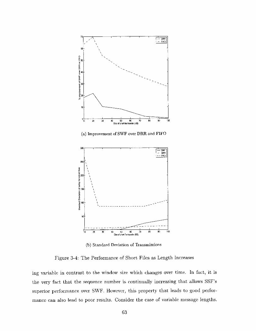
0
~50-
0
40
0
LL
-30
E
10 20 30 40 50 60 70 80 90 100Size of short file transfer (KB)
(a) Improvement of SWF over DRR and FIFO
300-SWF
-- DRR-FIFO
250
E200
5150 -.2
2100 -
50-
10 20 30 40 50 60 70 80 90 100Size of short file transfer (KB)
(b) Standard Deviation of Transmissions
Figure 3-4: The Performance of Short Files as Length Increases
ing variable in contrast to the window size which changes over time. In fact, it is
the very fact that the sequence number is continually increasing that allows SSF's
superior performance over SWF. However, this property that leads to good perfor-
mance can also lead to poor results. Consider the case of variable message lengths.
63
7n. I I I
The performance of the SSF scheduler heavily penalizes long connections, especially
those that begin early on in our time interval. SSF transmits the long session, k,
for a while before another session opens. Thus, k's packets have a large sequence
number. However, once new sessions arrive, k will not be able to transmit again until
all other active sessions have transmitted as many packets as it has. This is why, SSF
transmits packets from short term sessions rapidly, but long sessions have to wait out
a considerable amount of time. SWF on the other hand does not force long sessions
into long periods of idle. If a long term session times out after a packet drop due to
buffer over flow, its window will decrease dramatically, and it will be given priority by
the SWF scheduler. In fact in some cases, the performance of SWF for long sessions
is identical to that of DRR. However, there does need to be some outside pressure on
the congestion window to make the SWF work correctly.
As mentioned previously, the congestion window size, which determines the num-
ber of unACKed packets allowed in the network at any point in time, is much more
correlated to the number of packets the session currently has buffered than the se-
quence number. It is possible for a session to have a catastrophic failure, but still
have sequence numbers greater than other sessions simply because it has been run-
ning longer. So the ALQD policy used by the SWF is a truer version of the LQD
than SSF's ALQD.
3.3.5 Summary
We describe two new new active queue management schemes: Shortest Window First
(SWF) with Approximated LQD and Smallest Sequence Number First (SSF) also with
Approximated LQD. SWF and SSF are unique in that they rely on information other
than the source id and the number of buffered packets to make decisions on scheduling
and packet admission. Our queue management schemes make decisions and prioritize
packets based on a packet's TCP header. They extract information on the originating
sessions allowed number of unACKed packets and number of successfully delivered
packets using the congestion window size and sequence number, respectively. We
describe the benefits of our policies and provide simulation results to verify our claims.
64

We find that both SWF and SSF are capable of increased levels of goodput to lossy
sessions. SSF can also provide increased performance for isolated poorly performing
sessions with high propagation delays. Both schedulers are capable of transmitting
short messages with a latency that is substantially lower than that of current queue
management policies (FIFO with DropTail and DRR with LQD).
3.4 Scheduling Heuristics
Due to the potentially high complexity of the SWF scheduler, we explore the possibil-
ity of developing some heuristic approaches to SWF. In the methods detailed below,
we avoid sorting of any kind. This keeps per packet complexity low. The heuristics we
present are for SWF, but they can easily be considered SSF heuristics if the window
size metric is converted to a sequence number metric.
3.4.1 Random Insertion
In the Random Insertion queue management policy, packet headers determine where
in the queue, a newly arriving packet belongs. If the packet's source window size
is less than Wmin, the packet is randomly inserted into the queue using the uniform
distribution. If the packet is from a session with a congestion window greater than
Wmin, it is simply inserted at the tail of the queue in normal FIFO fashion. On
average, packets from sessions with window sizes less than Wmin will be inserted into
the middle of the queue. Thus somewhat reducing the queuing delay these packets
experience.
The packet admission policy is a modified version of DropTail. If a newly arriving
packet encounters a full buffer and the packet has a window size less than Wmin,
then the packet at the tail of the queue is dropped and the new packet is randomly
enqueued. If the newly arriving packet comes from a session with a window size
greater than Wmin, it is dropped. We had originally implemented the Random Inser-
tion policy with a simple DropTail mechanism. However, we quickly noticed that its
performance was not distinguishable from that of FIFO with DropTail when looking
65
at fairness. In the current implementation, we have something that is between a
DropTail and ALQD implementation in terms of performance.
The problem with the Random Insertion method is that it can lead to out of order
packet delivery. Packets from sessions with windows below the threshold are randomly
inserted into the buffer. Out of order delivery in an of its self is not a problem. The
TCP receiver is capable of buffering any out of order packets it receives. However,
TCP Reno issues an ACK for every packet is receives. Therefore, there is a danger of
duplicate ACKs being received at the TCP sender. The reception of duplicate ACKs
triggers fast retransmit and recovery, and the congestion window will be reduced as a
consequence. See Appendix A for more information. The packet reordering problem
becomes more severe as Wmin increases. However, as Wmin increases our scheduler
is able to grow the congestion windows of sessions that are just beginning or have
experienced a loss event more aggressively. Thus, there is an inherent tradeoff in
determining the correct value of Wmin.
The optimal threshold depends on a variety of factors, the number of active ses-
sions, the number of lossy sessions, the propagation delay, and the network congestion
etc. In addition, if networks change over time, as all wireless networks do, the value
of Wmin will need to be recalibrated. We do not know how to compute Wmin a priori.
3.4.2 Small Window to the Front Scheduler
Another approximation to the SWF is the Small Window to the Front Scheduler.
This scheduler is in a sense derived from the Random Insertion policy. The Random
Insertion scheduler could be improved by randomly inserting packets into the front
half of the scheduler instead of randomly inserting them into any location in the
queue. A natural extension is to let packets from sessions with window sizes less than
Wmin cut to the head of the line. Packets from sessions with congestion windows
greater than Wmin are simply enqued at the end of the queue. The packet admission
policy we implement is a modified DropTail. It is identical to the policy used in the
Random Insertion scheduler.
Depending on the size of the buffer, one of the potential problems with this sched-
66

uler, is the sharp increase in queuing delay sessions will experience. Packets that are
transmitted when the session has a window size less than Wmin experience virtually
no queuing delay. There is very little variation in the RTT. But when a session's win-
dow reaches the critical size of Wmin, its packets will be sent to the end of the queue.
Queuing delays will increase substantially, and can cause a timeout event, depending
on the size of the queue and the number of buffered packets. In the SWF scheduler,
packets move more slowly from the front to the back of the queue, minimizing spikes
in the RTT.
There is also a potential starvation problem if Wmin is set too high. Sessions will
be allowed to transmit large bursts of packets, after which they will have to wait a
considerable amount of time before the scheduler lets them transmit again.
3.4.3 Window Based Deficit Round Robin
The Window Based Deficit Round Robin (WDRR) scheduler deviates considerably
from the SWF scheduler. Rather than simplifying SWF, we alter DRR to behave more
like SWF. Instead of hashing packets into buckets based on their source, packets are
hashed into buckets based on their window size. However, questions quickly emerge.
How should the window size range for each bucket be determined? How should quanta
be allocated to the buckets? Should buckets with packets from sessions with smaller
congestion windows be allocated more quanta?
If the number of buckets is large and the the range of window sizes per bucket
small, then there is a danger of out of order packet delivery which can result in un-
necessary window closures as well as potentially unnecessary packet retransmissions.
Optimizing a WDRR system is non-trivial.
Each bucket is handled in a FIFO manner. Therefore, if buckets that contain
packets from sessions with small window sizes are not allocated more quanta, it is
conceivable that packets from a particular session will not be served in a FIFO manner,
although they would be if DRR were used instead. However, if buckets with small
window sizes are allocated more quanta, or can transmit more packets per round, a
starvation problem could arise.
67

One potential solution to this problem would be to hash packets into buckets based
on whether they are from a session that is in slow start or congestion avoidance.
Unfortunately, there are no fields for slow start or congestion avoidance in packet
headers. A new header would have to be added for this purpose.
Generally speaking, we find this policy infeasible. Calibrating the system is simply
too difficult.
3.4.4 Summary
The heuristic schemes we outline all have the potential to provide increased fairness
benefits over DRR and FIFO. In addition, the heuristic approaches have a lower
complexity than SWF with ALQD as well as DRR with LQD. However, they are very
dependent on network manager specified parameters like Wthresh. These parameters
are not easy to specify and for maximum performance need to be changed as the
network conditions change (RTTs change or channels become more or less lossy).
This is the primary reason, these heuristic methods are not as valuable as the SWF
scheduler, though they do provide some interesting alternatives.
3.5 Summary
In this chapter, we discuss queue management schemes. Queue management is im-
portant in determining the queuing delay packets from different sessions experience.
The queuing delay is one of the only parameters affecting the RTT that we can con-
trol. The propagation delay is largely determined by the transmission media and the
distances over which we are transmitting. Queue management is comprised of two
different parts: the scheduler and the packet admission policy. We discuss existing
queue management policies as well as our own. Both the SWF and the SSF sched-
uler with ALQD are innovative in their attempts to give packets from short lived
and lossy sessions an advantage in both the packet admission policy as well as the
scheduling algorithm. Existing queue management schemes that attempt to reduce
the latency of short sessions due so through the use of a specialized packet admission
68

policy [19]. Through the use of simulations, we show the advantage of using our queue
management schemes.
69

70

Chapter 4
TCP over Random Access
Protocols in Satellite Networks
In this chapter, we consider sessions that use random access protocols to gain access
to the satellite network. We introduce the the ALOHA family of protocols in greater
detail. Through the use of simulations, we try to gain intuition into the effect of
ALOHA on TCP's feedback and congestion control mechanisms.
4.1 Introduction
The study of TCP's interactions with MAC layer protocols remains relatively un-
touched. Gerla et al. studied the performance of TCP over CSMA in multihop adhoc
networks [18]. They found that the use of TCP in conjunction with CSMA dramati-
cally reduces throughput when the window size is greater than one. If the window size
is greater than one, data packets and ACKs can collide. Also as the TCP window size
grows, the system load increases and there are more collisions. Unfortunately, their
study concentrates more on how the number of hops in the network effects perfor-
mance, rather than on the actual interaction between the MAC and transport layers.
One recently developed MAC layer protocol designed to operate with TCP is a com-
bination of TDMA and Bandwidth on Demand (BoD) [29]. STP, a modified version
of TCP, was designed for point-to-point links. However, the designers of TDMA-BoD
71

extend STP for the case where multiple sessions share the same uplink. Terminals
are allowed to request slots every 250msec, approximately half the round trip time
of satellite links. If there are any remaining, unclaimed slots, they are distributed
to the terminals. The distribution occurs in such a fashion that the terminal that
currently has the highest load receives more free slots. This multiple access protocol
is reservation based, as such there are no real MAC/TCP layer issues to discuss. TCP
ACKs are sent across the satellite links as well. Their transmission is governed by
the STP protocol.
4.2 Random Access Protocols
The most common random access protocols are the ALOHA family of protocols and
CSMA. CSMA is used in the ethernet standard and can be considered to be a modified
version of ALOHA. Packets cannot be transmitted if the channel is "sensed" to be
busy. Nodes will transmit a packet with a certain probability p when they detect
that the channel is idle. Unfortunately, in satellite networks, propagation delays are
high. The time to detect whether or not a node is transmitting is large. While CSMA
remains one of the most popular MAC layer protocols for LANs, it is not appropriate
for high delay satellite networks. Hence, we focus our attention on the ALOHA family
of protocols.
4.2.1 Assumptions made in ALOHA analysis [6]
" Slotted System. All packets are the same length, and require a unit of time or a
slot for transmission. All transmitters are synchronized; they see the same slot
start and end times.
" Poisson arrivals. Packets arrive for transmission at each of the m nodes ac-
cording to a Poisson process. A is the overall system arrival rate, with A/m the
Poisson arrival rate at each node.
72
" No capture. Analysis assumes no capture. If more than one packet is sent in
the same slot, a collision occurs. None of the packets involved in the collision
are successfully received. If only one packet is sent in a given interval, it is
successful.
" Immediate feedback. At the end of a slot, each node learns what the status of
the slot was from the receiver. It could either have been idle, successful, or
collision.
* Retransmission. Each packet involved in a collision must be retransmitted at
some point. In fact, each packet must be retransmitted until it is correctly
received. A node with a packet that requires retransmission is referred to as a
backlogged node.
" Infinite nodes/no buffering. There is no MAC layer buffering. If a packet is at
a node awaiting transmission or retransmission, newly arriving packets will be
dropped. These dropped packets will never be transmitted, unless they are sent
down to the MAC layer by a higher layer again. Conversely, one can assume
that there are an infinite number of nodes, so each newly arriving packet will
arrive at a new node. Therefore, there is not need for a MAC layer buffer.
4.2.2 Implications of Assumptions
Assuming a slotted system makes analysis substantially easier. The assumption of
Poisson arrivals is not accurate especially when considering the fact that packets need
to be retransmitted. In real system implementations, there are only a finite number
of nodes. The number of packets needing retransmission can dominate the newly
arriving packets, if the probability of collision is high and the data rate is low.
The no capture model ignores the fact that there could be bit errors in the channel
which could result in loss. It also ignores the fact that nodes can sometimes still
receive and reconstruct "collided" packets.
The immediate feedback assumption is the most unrealistic assumption made for
73
the purposes of analysis. It is especially unrealistic in satellite channels, where round
trip delays can exceed half a second. It would take a node in a satellite network at
least half of a round trip time to determine if a collision occurred. If a node were
to wait for feedback before it transmitted its next packet, throughput would suffer
substantially. In implementation, one typically has to assume all packet transmissions
were successful until it is confirmed otherwise.
The retransmission assumption is fairly reasonable, except for the fact that it
allows for an infinite number of retransmissions. In practice, it is likely that there
would be a fixed number of allowable retransmissions. The MAC layer would be
expected to stop retransmissions at some point, leaving the higher layers to discover
the loss, and accept new packets for transmission.
The no buffering assumption is problematic because packets may need to be re-
transmitted. Nodes that have packets requiring retransmission are considered to be
backlogged; they cannot accept new packets. In practical systems, some buffering
is always necessary. Analysis typically considers the case where, m, the number of
nodes is large and A, the system data rate, is small. Thus, each new packet arrives at
a new node that has not received a packet yet. The infinite node assumption provides
a pessimistic analysis - an upper bound on delay.
4.2.3 slotted ALOHA
In slotted ALOHA, each unbacklogged node transmits newly arriving packets in the
next slot after their arrival. In a system with a low data rate, packets experience
few collisions and low delays. This is in marked contrast to TDMA systems where in
large systems nodes may have to wait a considerable amount of time before it is their
turn to transmit.
However, in multiple access systems like ALOHA, collisions may occur when sev-
eral nodes attempt to transmit in the same slot. When a collision occurs, a node
becomes backlogged. It will not accept any new packets, and will retransmit the
collided packet after some random amount of time. It is essential that the node wait
a random amount of time, if it were to wait a fixed number of slots before retrans-
74
mission, another collision would likely occur. We refer to this idle time as the backoff
time.
Analysis of ALOHA begins with the construction of an attempt rate. The attempt
rate, refers to the expected number of transmissions that are attempted within a given
time slot. The attempt rate, G(n), is a function of the number of backlogged nodes,
n.
G(n) = (m - n)qa + nq,, (4.1)
where qa refers to the probability that an unbacklogged node attempts a transmission
and q, refers to the probability that a backlogged node will retransmit its packet.
The probability that an unbacklogged node will transmit a packet is governed by the
system arrival rate, q, = 1 - e-A/m. The value of q, is set by the network manager,
and may be optimized on a per network basis. A packet is successfully received if one
and only one node, backlogged or unbacklogged, transmits in a slot. This probability
of success in slotted ALOHA can be approximated fairly accurately by the following
expression,
PS = G(n)e-G(n). (4.2)
Since at most only one packet can be successfully received per slot, the throughput
of slotted ALOHA is simply the P,,c,. The maximum throughput of slotted ALOHA
is e- 1 .
4.2.4 unslotted ALOHA
Unslotted ALOHA was developed before slotted ALOHA. However, the discrete na-
ture of slotted ALOHA makes it easier to analyze, thus we considered it first. In
unslotted ALOHA, as the name suggests, there are no slots. So the assumption of
a slotted system in the previous section can be ignored, however, all of the other
assumptions still hold. Nodes transmit newly arriving packets as soon as they are
received. If a packet is involved in a collision, the node becomes backlogged and
enters backoff for a random amount of time, and then retransmits the packet.
Without slots, the probability of collision increases dramatically. If any two nodes
75

transmit at the same time, a collision will occur, but if the transmission of any two
nodes overlap a collision will also occur. If the transmission time of a node is one
unit and transmission begins at time t, the transmission will only be successful, if no
other transmissions begin in the interval from t - 1 to t + 1.
As before, n refers to the number of backlogged nodes. Nodes are considered to be
backlogged from the moment a collision has occurred. The attempt rate for unslotted
ALOHA becomes
G(n) = A + nx, (4.3)
where A is the system arrival rate and x can be considered the retransmission attempt
rate (it follows an exponential distribution).
Only one node can transmit in an interval of two units if a success is to occur.
The probability of success is said to be
Sc = e 2 G(n) (4.4)
Since at most only one packet can be received in a time unit, the throughput becomes
G(n)e- 2G(n). Thus, unslotted ALOHA has substantially smaller throughput than
slotted ALOHA. In fact, the maximum throughput is exactly half that of slotted
ALOHA. However, it is easier to implement since neither synchronization nor fixed
length packets are required.
4.2.5 p-persistent ALOHA
The design of p-persistent ALOHA builds upon the slotted ALOHA model. How-
ever, p-persistent ALOHA also bears several similarities to CSMA protocols. In the
original version of CSMA, newly arriving packets that arrive during an idle period
are transmitted at the start of the next available slot. If they arrive during a busy
period, they are transmitted at the at the end of the current slot. This can lead to
many collisions. Hence, p-persistent CSMA was developed. In p-persistent CSMA,
collided packets and new packets wait until the end of the busy period to transmit.
76

Collided and new packets have different probabilities of transmission.
ALOHA, theoretically, has the ability to determine the state of the channel after
transmission has occurred. It does not however, have the ability to sense the channel.
CSMA does, that is how it knows whether or not a slot is busy or idle before trans-
mission occurs. In the original version of slotted ALOHA, newly arriving packets
are transmitted at the beginning of the next available slot. In p-persistent ALOHA,
newly arriving packets are transmitted with probability p at the next available time
slot. Thus, slotted ALOHA and 1-persistent ALOHA are one in the same.
When packets experience a collision, sessions backoff for a random number of
slots before attempted to resume transmission in the next slot. The p in p-persistent
ALOHA refers to the probability with which a new packet is transmitted. It does not
refer to the probability with which a backlogged packet is transmitted, which we will
refer to as q. Optimizing performance of a p-persistent system over p is non-trivial.
The optimal value of p depends on many factors including the total system load and
q.
The attempt rate of p-persistent ALOHA is potentially much lower than that of
slotted ALOHA. It becomes
G(n) = (m - n)qap + nq, (4.5)
where the definition of all variables is identical to that of equation 4.1. The effect
of p is evident in the attempt rate equation. The smaller p is the more time elapses
between new transmissions. This potentially lowers the number of collisions in the
network. Unfortunately, it also has the effect of reducing the network throughput
since packets are held at the MAC layer for longer periods of time. Just as in slotted
ALOHA, the throughput of the p-persistent system follows equation 4.2.
77

4.3 Implementations of ALOHA in ns - 2
The satellite network implementation of ns -2 provides a MAC layer implementation
they call unslotted ALOHA. Unfortunately, this implementation is not an accurate or
practical version of unslotted ALOHA. The ns - 2 implementation has no MAC layer
buffer, following the theoretical guidelines. However, it lacks instantaneous feedback.
Therefore, the transmitter has to wait roughly RTT/2 before learning the status
of its last transmission. It takes RTT/2 seconds to discover whether a collision has
occurred since only the uplink is contention based. The ns-2 version of ALOHA waits
until it learns the status of the last transmission before transmitting the next packet.
Although this prevents packets from being transmitted out of order, it does not make
efficient use of bandwidth, and it constrains the achievable goodput. In addition,
out of order reception at the transport layer will not cause the system to collapse
either. The TCP receiver is able to buffer packets, with sequence numbers between
the last ACKed packet and the last ACKed packet + advertised window, that
arrive out of order. Excessively delaying transmission, only serves to limit achievable
throughput.
The instabilities present in theoretical ALOHA are not evident in ns -2 ALOHA.
Packets can not be released at a rate greater than one per RTT/2. Thus, 2/RTT is
the critical data rate. If the external arrival rate is exceeds the the critical data rate,
the data rate seen by the MAC layer will not exceed the critical data rate.
We augment the ns - 2 implementation of ALOHA to create both an unslotted
and a slotted ALOHA implementation. We focus on slotted ALOHA in this thesis.
The first step is to create the notion of a slot. Since we use fixed length packets, a slot
is equal to the transmission time of a data packet. (ACKs, which are smaller, may
have slightly delayed transmissions.) Another important extension was the creation
of a MAC layer buffer. In our system, when a node is not in backoff, the MAC layer
accepts packets until its buffer is full. The MAC layer transmits packets in the order
they were received. We do not wait for feedback on the success of failure of the last
transmission before transmitting the next packet. This allows us to efficiently use
78

the channel bandwidth and transmit more data. However, it substantially increases
the likelihood that packets will be delivered out of order. Out of order delivery can
result in the reception of duplicate ACKs leading to the closure of the TCP congestion
window.
A node enters backoff upon realizing that a collision has occurred. While in backoff
the MAC will not request any packets from the higher layers. Packets are effectively
blocked from entering the MAC layer of a node when it is in backoff. Instead packets
will build up at higher layers, namely either the TCP or the application layer. Our
backoff policy is identical to the one considered in analysis. While in backoff, a node
can not transmit any packets. The duration of the backoff period is an exponentially
distributed random variable. At the end of the backoff period, the node will first
transmit the collided packet followed by any other packets residing in the MAC layer
buffer after which transmission proceeds normally. In later sections, we compare
different values of the mean backoff time. When referring to the mean backoff time in
our description of p-persistent ALOHA, we used the parameter q. q is the probability
a packet will be retransmitted in the next slot given that it just experienced a collision.
However, in our simulations, we do not use q, we instead use the mean duration of
the backoff period. The mean number of slots can be related to q using the following
expressions. Using q, the distribution of the backoff period would be
p(n) =q(-q)" n= 0,1, ... , (4.6)
where n is the number of slots spent in backoff. This is really just the geometric
distribution. So using q, the average number of slots a session spends in backoff is
N = 1/q. (4.7)
N is the expected number of slots a session would spend in backoff after a collision.
Each time a collision occurs, in our simulations, we compute the mean backoff time
by generating an number using an exponential distribution with mean N. The expo-
nential distribution is the continuous version of the geometric distribution. Since the
79

exponential distribution is continuous, it can take non-integer values. Therefore, we
have to discretize the number of slots that comprise the backoff interval.
We discover that using slotted or 1-persistent ALOHA provides the greatest good-
put. Values of p less than one do not provide as high performance. Therefore, in our
simulations, we consider a slotted ALOHA system exclusively.
Finally, in our model, ACKs travel across the same channel as data packets. There-
fore, it is possible for ACKs and data packets to collide. In most commercial satellite
systems, one example being DirectPC, communication occurs over fixed access chan-
nels. Collisions are not a concern. We consider the point-to-point case in Chapter
3. In DirectPC type implementations, ACKs are sent across low propagation delay
terrestrial links. When downloading large files, this can reduce congestion on the
reverse channel. Given the throughput of ALOHA, we know the combination of TCP
and ALOHA will only be able to support low data rates. It is unlikely that people
would use an ALOHA based system system to download large files. The delays would
simply be too large once collisions are factored in. We believe the applications of a
TCP/ALOHA network are more pertinent to sensor networks and remote communi-
cations. In these applications, short messages are sent out periodically. The network
is not heavily loaded and the number of collisions are minimized. If such systems
were used for tactical communications and surveillance, there can be no assumption
of existing terrestrial infrastructure. Therefore, we feel justified in assuming that
ACKs do not travel across high speed point-to-point links. In addition, most simula-
tion studies assume that ACKs return to the TCP source over satellite links if data
packets travel over satellite links.
4.4 Interactions between TCP and ALOHA
We are interested in several different parameters. The TCP window size, W, the round
trip time, RTT, which is used to compute the TCP time out interval, the probability
of collision, Pc0u, and R, the maximum number of MAC layer retransmissions allowed
before discarding the packet. If the MAC layer discards a packet, TCP must discover
80

the loss either through duplicate ACKs or a RTO. The probability that the MAC
layer will stop retransmitting a packet is specified by P 11, the probability that a
packet experiences R collisions. P&1 is also roughly speaking the " probability of
error" or the "congestion level" seen by the transport layer, TCP.
The TCP window size, W, is affected by the probability of error which we approx-
imate as PLI. Depending on the Pc0u and the data rate, a session may experience
a greater number of RTOs or duplicate acknowledgments. However, the probability
of collision is affected by the system load, which is proportional to the window size.
TCP is allowed to release no more than W packets per RTT. This suggests the prob-
ability of collision and the window size grow inversely. Pc,,, can also be affected by
the backoff policy the network manager implements. If the backoff interval is not
selected with care, collisions can occur at retransmission due to synchronization.
The round trip time is an important quantity in computing the system load.
It depends on several MAC layer parameters: the backoff policy, the probability of
collision, and the number of MAC layer retransmissions allowed. The RTT is specified
by the following equation,
RTT = 2Dprop + Dtx + B( -1), (4.8)1 - Pcou
where Dprop is the one way propagation delay, Dtx is the transmission delay, and B
is the expected backoff time. We ignore the queuing delay since ALOHA assumes no
buffering, though in actuality it could play an important role.
The MAC layer parameter, R, can actually improve system goodput. Retransmis-
sions allow the MAC layer to recover from losses before TCP realizes that they have
occurred. We hypothesize that MAC layer retransmissions depend on the backoff
policy. If the mean backoff time is too large, it might be better for TCP to discover
all losses on its own. We also believe that the TCP congestion window will shape
the data rate seen by the MAC layer. This should prevent the instabilities of basic
ALOHA from arising.
81
4.5 Optimizing slotted ALOHA performance over
TCP
In this section, we select optimal values for both ALOHA and TCP parameters in
order to ensure high goodput. We consider network manager defined parameters
including the number of MAC layer retransmissions, the mean backoff time, and
the advertised TCP window size. In addition, we provide intuition as to why our
selections are correct.
In our simulations, we consider the performance of ten TCP sessions. The source
and destination are connected via a geostationary satellite. Ground terminals share
a random access uplink of 1Mbps; the downlink is also 1Mbps. Sessions transmit
packets that are 1000 bytes in length. The transmission time, Dt, for these packets
is 0.008128 seconds. Thus, each slot is Dt. seconds long. We consider the performance
of both a heavily loaded as well as a lightly loaded system. In the highly loaded case,
each of the ten sessions has an application layer data rate of 40Kbps, for an aggregate
system load of 400Kbps. While in the lightly loaded case, sessions have an application
layer data rate of 8Kbps, for a system load of 80Kbps. All the traffic that we consider
in our simulations is Poisson in nature. The application layer generates packets with
exponential interarrival times.
We briefly mention a few points of interest. Slotted ALOHA's backoff policy needs
to be finely tuned. At high data rates where the packet interarrival time and the slot
duration are roughly equal, if the mean backoff time is not sufficient large, there is
excessive synchronization. The retransmission of "collided" packets will result in yet
another collision. However, there is an inherent trade-off in setting the mean backoff
time. If it is too large, goodput will suffer since nodes will idle for long periods of
time. However, if it is too small, collisions will result, which again forces connections
to spend far too much time in backoff. In fact, if the mean backoff time is too large, it
is possible for lightly loaded sessions to achieve a greater goodput that heavily loaded
sessions.
We notice that the combination of TCP and slotted ALOHA does not provide
82

large goodput. Slotted ALOHA itself can only provide a maximum throughput of
up to 36%. However, our combined slotted ALOHA/TCP implementation provides
a maximum throughput of no more than 13%. Still at low loads, we manage to
successfully transmit the entire load.
4.5.1 Selecting a Backoff Policy
We implement an exponential backoff policy at the MAC layer. If a collision occurs,
the sessions involved must wait an exponentially distributed amount of time before
transmitting again. Therefore, when discussing backoff policies, we always speak in
terms of the mean backoff time. The optimal backoff policy in the heavily loaded
case varies between five and ten slots. There appears to be a dependence between the
optimal mean backoff time and the maximum number of allowed MAC layer retrans-
missions. If the mean backoff time is too small, for example one slot, synchronization
problems can result. With high probability, sessions that experience a collision will
backoff and retransmit in the next slot, thus incurring another collision. However,
if the mean backoff time is too long, more than twenty-five slots, for each collision
that occurs, a session will spend a considerable amount of time in backoff. When a
session is in backoff, it cannot transmit any packets. Thus, fewer transmissions are
attempted and goodput suffers. Therefore, from a goodput perspective, an average
mean backoff time between five and ten slots is ideal. See Figure 4-1(a) for the case
where the system is heavily loaded, and the maximum congestion window size is 100
packets.
In the case of a lightly loaded system, the choice of the mean backoff time does not
have as significant of an effect on goodput. Provided that the mean backoff time is
not too large, the system goodput is equal to the system load. However, as the mean
backoff time increases, we encounter the same problem we did in the heavily loaded
case. Too much time is spent in idle and fewer transmissions are attempted. See
Figure 4-1(b), for a lightly loaded system with a maximum congestion window size
of 100 packets. We do not find that short mean backoff times affect system goodput.
Synchronization is not as much of a problem in the low data rate case since packets
83

0.13
0.12 r
0.11 -
0.1
o 0.09-0
0.08-
0.07 -
0.06-
0.050 10 20 30 40 50 60 70 80 90 100
Mean Backoff Time (slots)
(a) Heavily Loaded System
0.00
-R=5
0.075
0.07
E0.065-
0.06
0.055'0 10 20 30 40 50 60 70 80 00 100
Mean Backoff Time (slots)
(b) Lightly Loaded System
Figure 4-1: The Effect of the Mean Backoff Time on System Goodput
are not arriving as rapidly. In the heavily loaded case, system packet interarrival
times are on the order of two time slots. In the lightly loaded case, system packet
interarrival times are on the order of ten slots.
Note that at R = 0, the mean backoff time has no effect on goodput. Packets are
84
- R=0R-=2R=5

never retransmitted and nodes are never backlogged. TCP must discover all collisions
on its own. However, for R not equal to zero, there are cases where the backoff policy
is so poor, that lightly loaded sessions will have a higher goodput than heavily loaded
sessions. We will return to this topic again when we discuss TCP and MAC layer
interactions.
4.5.2 Selecting an Advertised Window Size
The advertised window size affects system goodput. The window size advertised by
the TCP receiver limits the maximum congestion window size. It imposes flow control
on the system. The larger the advertised window size, the more traffic the receiver is
able to support. The TCP congestion window shapes traffic received from the MAC
layer, specifically in the case where the application data rate is greater than the rate
the congestion window can support. Small advertised window sizes constrain the
growth of the TCP congestion window and effectively limit the rate at which sessions
can transmit packets. If the maximum advertised window is one packet, it is the same
as having no MAC layer buffer. TCP will not hand the MAC layer a new packet until
the current packet is successfully transmitted and ACKed. We find that an advertised
window size of six packets or larger tends to provide the highest performance. See
Figure 4-2 for the case where the aggregate system load is 400Kbps, and the mean
backoff time is five slots.
Goodput stabilizes with increasing advertised window size. At some point, the
advertised window size does not matter since the congestion window will never be
large enough to be constrained by the receiver's advertised window. Since packets
experience MAC layer collisions, TCP will on occasion experience loss events. These
loss events cause the TCP congestion window to close. The TCP window, which we
almost always refer to as the congestion window, size equals
min(congestion window, advertised window). With MAC layer losses and a large
advertised window, the TCP window size will always be set by the congestion window.
Thus, the flattening of the goodput curve is due to loss events not the advertised
window size which is too large to have any effect.
85

0.13 R 0
R=2
0.11
o 0.1 -
E
0.09-
0.08 --
0 10 20 40 60 70 80 90 100TCP Advertised Window Size (packets)
Figure 4-2: The Effect of the Advertised Window Size on System Goodput
4.5.3 Selecting the Number of MAC Layer Retransmissions
MAC layer retransmissions can enhance system goodput. As R increases, sessions
have more opportunities to retransmit their data before TCP discovers that a loss
has occurred. TCP takes on the order of a RTT (the round trip propagation delay
of a GEO satellite is roughly 500msec), approximately 50 slots, to discover a loss.
This provides the MAC layer with ample time to retransmit the packet without
invoking TCP's congestion control algorithm. When R is equal to zero, no MAC
layer retransmissions are allowed. TCP must discover all loss events. TCP will
repeatedly enter fast retransmit and slow start due to loss events. This will cause the
congestion window to be closed often.
If the mean backoff time is too large or too small, MAC layer retransmissions are
not helpful. At low mean backoff times and large R, this is due to synchronization.
At high mean backoff times, the RTT to deliver a packet can substantially exceed
the timeout interval of TCP when R = 0. The long delay reduces goodput. This is
evident in Figure 4-1.
MAC layer retransmissions will improve goodput (as long as the mean backoff
time is not too large). See Figure 4-3, where the mean backoff time is ten slots and
86

0.1
0.12-
0.11 --
0.1 --
0.09
0.08. -
0.07 -
0.060 0.5 1 1.5 2 2.5 3 3.5 4 4.5 5
maximum # of MAC layer retransmissiis
Figure 4-3: The Effect of MAC Layer Retransmissions on System Goodput
the advertised window size is 100 packets. TCP will adjust to the changing RTT
caused by MAC layer retransmissions. Retransmissions will allow the MAC layer
more opportunities to successfully transmit a collided packet. TCP is not forced to
discover the loss on its own. Although increasing R helps goodput, we find that there
are diminishing returns. For every successive increase in R there is a smaller increase
in terms of goodput.
4.5.4 Goodput vs Load
When we refer to the system load, we refer specifically to the aggregate data rate
of each of the source's application layer. The application layer generates data at a
certain rate, A, and attempts to pass packets to TCP at this same rate, A. TCP
then passes packets to the MAC layer for transmission. Therefore, the load seen by
the MAC layer is not necessarily the load provided by the application layer. The
MAC layer sees TCP's offered load. When the congestion window is large and can
support the application data rate, TCP's offered load is the same as the application
layer's load. However, when the congestion window is small and the application rate
high, TCP acts like a funnel. It only allows a window's worth of unACKed packets
87
s~mload 80Kbpssstem toad 8Kbps
3

down to the MAC layer at a time. The remaining packets are backlogged between the
application and transport layers. We will return to the concept of the offered load in
the next section when we discuss the interaction of MAC and TCP parameters.
Our results show that TCP stabilizes the performance of ALOHA. See Figure 4-
4(a), where the mean backoff time is five slots and the advertised congestion window
size is six packets. We plot the system goodput versus the system load. In theoretical
slotted ALOHA, system goodput is typically defined as a function of attempt rate as
in equation 4.1 and looks like Figure 4-4(b). The attempt rate is really a measure
of the load. However, in our case, goodput does not decrease with system load. We
hypothesize that this is due to the following reasons. Theoretical ALOHA analysis
assumes an infinite number of nodes. Each packet arrives at a new unbacklogged
node and is transmitted in the next slot. So the MAC layer load is equal to the
aggregate network application load. However, in our case, the network load is not
equal to the MAC load. Due to practical limitations, we can only support a finite
number of nodes. This constrains the number of packets that can be transmitted per
slot. In addition, TCP shapes the network load using its congestion window. Given
that ALOHA creates a very lossy environment, the TCP congestion window will be
small regardless of the application layer data rate. Therefore, at some point, despite
the increasing session load, the TCP offered load will stay the same. Thus, system
goodput also stays the same. Through simulation, we find that TCP over ALOHA
cannot support data rates in excess of 120Kbps, in the case where we have 1Mbps
links and ten sessions. TCP cannot provide goodput any higher than roughly 12%.
It is worth noting that we do not count the acknowledgments in our goodput. If
we did, our goodput would be higher. In addition, there is a possibility that packets
may be delivered successfully multiple times. However, in our goodput calculations,
we would only count the transmission once. We will return to this topic in the section
on wasted transmissions.
88

0.12F
0.1
0.08 -
C1
5 0.06
0.04
0.02
00 0.2 0.4 0.6 0.8 1 1.2 1.4 1.
load (Mbps)
(a) Simulation Goodput
0.35
0.3
0.25
0.2
0.15
0.1
0.05
0 0.5 1 1.5 2 2.5 3attempt rate (pkts/slot)
3.5 4 4.5 5
(b) Theoretical Goodput
Figure 4-4: Simulation and Theoretical plots of System Goodput vs Load
4.5.5 Effect of the Number of Sessions
We try to understand how system goodput varies as the number of sessions contending
for the same link increases. In our simulations, the advertised TCP congestion window
89
6

size is 100 packets and the application layer data rate for each session is 40Kbps. We
find that as the number of sessions increases, the achieved goodput drastically diverges
from the ideal goodput. As the number of sessions contending for the link increases,
the system load also increases and so does the probability that more than one session
will attempt to transmit a packet in the same slot. This increase in the number of
collisions is what leads to the increased deviation between the ideal goodput and the
achievable goodput. Another interesting feature is that as the number of sessions
increases, the achieved goodput flattens out and slowly decreases. See Figure 4-5 and
Appendix C, where the mean backoff time is five slots. As the number of sessions
increases, the individual goodput achieved by each session decreases. This decrease
in individual goodput is due to the increase in the system load which increases the
number of collisions.
10,I-actual i;;5Fput
100
10-20 5 10 15 20 25 30
number of sessions
Figure 4-5: The Affect of the Number of Sessions on Goodput
4.5.6 Summary
The combined TCP/ALOHA goodput depends on several factors, the number of MAC
layer retransmissions, the receiver advertised maximum TCP window size, and the
mean backoff time. We attempt to select the optimal values of each of these variables
90

in the case where we have ten TCP sessions transmitting across a random access up-
link of 1Mbps. We find that when the system is lightly loaded, these variables do not
need to be selected as precisely. However, when the system is heavily loaded, proper
selection of these parameters is crucial. Results are the best when the advertised win-
dow size is not too small. It prevents the TCP congestion window from ever getting
too large and prevents the occurrence of burst errors. In most cases, increasing the
number of MAC layer retransmissions increases the overall system goodput. Finally,
when selecting a backoff policy, it is vital that the mean backoff time be neither too
large or too small. We settle on a mean backoff policy between five and ten slots. We
also show that TCP stabilizes the performance of ALOHA. As in Gerla et al. [18], we
have ACKs traveling across the same channel as TCP data packets. However, they
claim that if the TCP window size is greater than one, the goodput of the combined
TCP/CSMA system decreases. We do not find that to be the case. In fact, we find
that there is a sharp increase in goodput when the TCP congestion window is allowed
to take values greater than one. Our results indicate that setting the TCP congestion
window to be small can lead to worse goodputs than the case in which congestion
windows can take large values. Even if the maximum possible TCP window size is
constantly increased, goodput stabilizes. Collisions ensure that congestion windows
do not grow excessively large.
4.6 Simulating Interactions between ALOHA and
TCP
In this section, we attempt to understand the relationship between TCP and MAC
layer parameters. One of the most important TCP parameters is the round trip
time. The RTT is used to set the timeout interval. It determines the speed with
which TCP can detect and recover from losses. The RTT, as we will discuss, also
plays a significant role in determining TCP's offered load. The most important MAC
layer parameters are R, the maximum number of MAC layer retransmissions, and the
91

mean backoff time. As shown in equation 4.8, they play a large role in determining
the round trip time. Another parameter of interest is the probability of collision.
The probability of collision depends on a variety of factors, the TCP window size,
the number of active sessions, and the mean backoff time, as well as R. We attempt
to understand the probability of collision's dependence on each of these variables. As
before, we consider ten TCP sessions transmitting over a satellite link. The uplink
and downlink are 1Mbps each.
4.6.1 Round Trip Time
The round trip time increases, as expected, with both R and the mean backoff time.
This is obvious from equation 4.8. However, it also makes sense intuitively. If the
MAC layer attempts R retransmissions before discarding a packet, the packet in
question will spend extra time awaiting retransmission in the MAC layer buffer. This
waiting time, the mean backoff time, pads the TCP estimate of the round trip time.
If there were no MAC layer retransmissions, the "collided" packet would simply be
lost. Upon realization of the loss, TCP retransmits the packet. The packet header
will contain a new time stamp. Thus, the round trip time, in the case, where R equals
zero would not be inflated due to the collision. Therefore, as either R or the mean
backoff time increases so does the round trip time. See Figure 4-6(a), for the average
RTT of a session when the system is heavily loaded, 400Kbps.
In addition, as either R or the mean backoff time increases, the variance of the
round trip time increases as well. See Figure 4-6(b) for the RTT variance, in the case
where the data rate is 0.4Mbps. When the mean backoff time increases, there is a
wider range of values over which sessions can backoff. In addition, as R increases,
packets can spend various amounts of time in the MAC layer buffer depending on
how many times they have collided. Since both the RTT and the RTT variance
increase with R and the mean backoff time, the TCP timeout interval will as well.
TCP learns the MAC layer behavior over time and adjusts its backoff mechanism so
that its congestion control and retransmission mechanism will not interfere with that
of ALOHA.
92
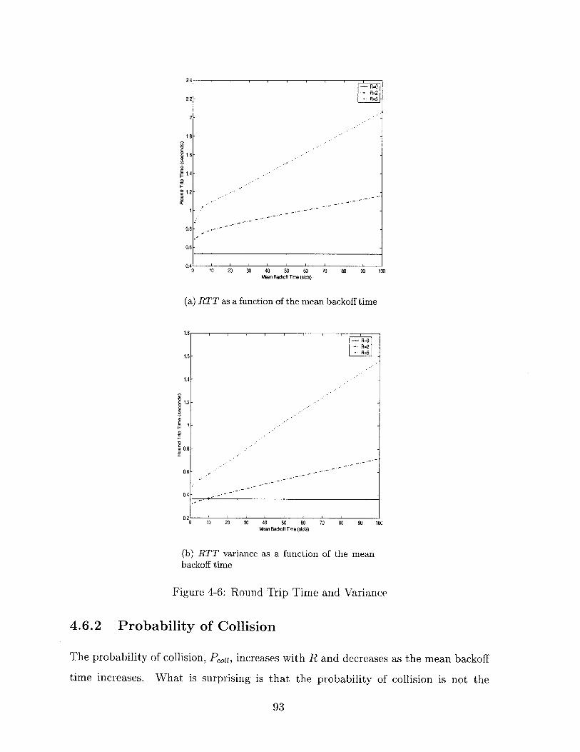
0.410 10 20 30 40 50 60 70 80 90 10
Mean Backoff Time (slots)
(a) RTT as a function of the mean backoff time
1.813=0
---R=2
1.6 - - R=5
1.4-
1.2
0.8-
0.6
0.4 - ..--
0 10 20 30 40 50 60Mean Backoff Time (slots)
(b) RTT variance as a functionbackoff time
70 80 90 100
of the mean
Figure 4-6: Round Trip Time and Variance
4.6.2 Probability of Collision
The probability of collision, Pc,,,, increases with R and decreases as the mean backoff
time increases. What is surprising is that the probability of collision is not the
93
I R=0-- R=2- -R52.2
2
1.8
0 1.6
1.4
'C 1.2
1
0.8
0.6
r
1
I-
"4z . 1
0

highest when the mean backoff time is equal to one slot. Due to synchronization
problems, we would expect the probability of collision to be the highest. Instead,
the probability of collision is the highest when the mean backoff time is between five
and ten slots. This range of mean backoff times also interestingly corresponds to
the highest system goodput. When the mean backoff time is one slot as opposed
to five slots, there is not sufficient time for backlogs to develop. Therefore, there is
not a burst of retransmissions following the the retransmission of the collided packet.
However, as R increases, for the case of the mean backoff time equal to one slot, there
is an opportunity for a backlog to develop, hence the higher probability of collision.
See Figure 4-7, for the probability of collision when the network is heavily loaded.
However, as expected, the probability of collision decreases as the mean backoff time
increases. With large mean backoff times, it is less likely that two or more sessions
will attempt to send a packet in the same time slot. However, when a collision does
occur, the session will spend a considerable amount of time in backoff, during which
time it will not be transmitting packets or causing collisions.
Introducing MAC layer retransmissions increases the probability of collision dra-
matically. Although there are small changes in the probability of collision for different
mean backoff times, R appears to have a greater impact. This is due to the build
up of packets between the TCP and MAC layer while sessions are in backoff. When
the backoff period is over, sessions will retransmit the collided packet and any other
packets awaiting transmission at either the TCP or MAC layer. This burst of traffic
increases the probability of collision. Another effect of large R is an increased load.
As R increases, the number of potential MAC layer transmissions also increases. The
larger MAC layer load can increase the probability of collision.
4.6.3 Collision Discovery
One might naively expect that as the mean backoff time or R increases so to do
the number of retransmission timeouts. However, we find the reverse is true. The
percentage of collisions discovered through timeouts does not significantly vary with
either the mean backoff time or R, provided that R is greater than zero. When R is
94
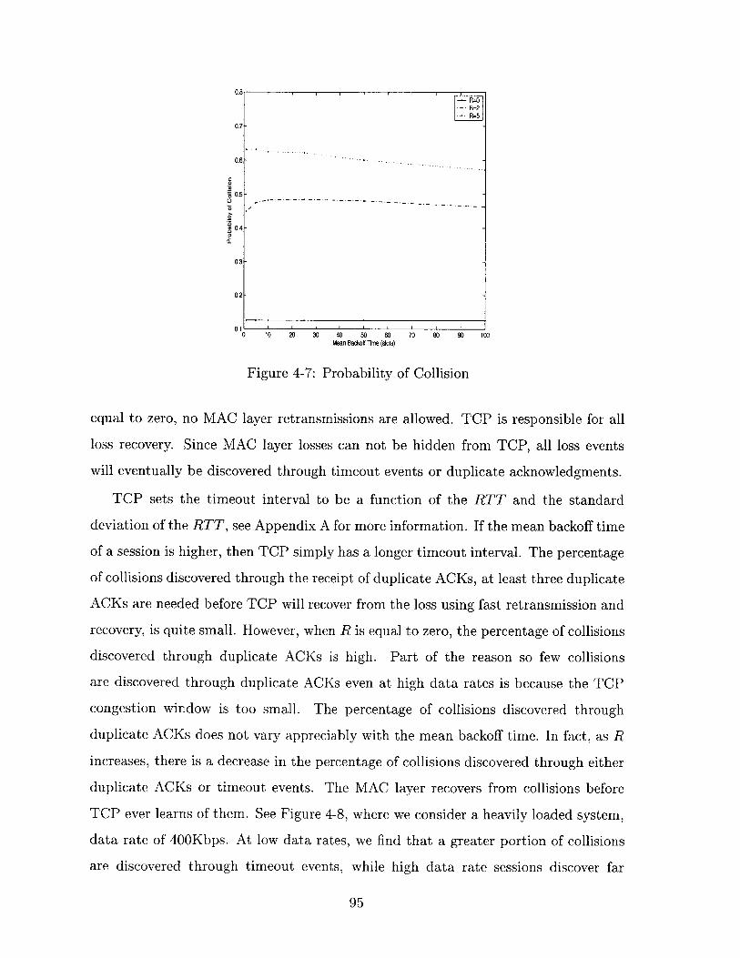
-R=0
0.7
0.6
0.5
0.4
0.3-
0.2-
0.10 10 20 30 40 50 60 70 80 90 100
Mean Backoff Time (sots)
Figure 4-7: Probability of Collision
equal to zero, no MAC layer retransmissions are allowed. TCP is responsible for all
loss recovery. Since MAC layer losses can not be hidden from TCP, all loss events
will eventually be discovered through timeout events or duplicate acknowledgments.
TCP sets the timeout interval to be a function of the RTT and the standard
deviation of the RTT, see Appendix A for more information. If the mean backoff time
of a session is higher, then TCP simply has a longer timeout interval. The percentage
of collisions discovered through the receipt of duplicate ACKs, at least three duplicate
ACKs are needed before TCP will recover from the loss using fast retransmission and
recovery, is quite small. However, when R is equal to zero, the percentage of collisions
discovered through duplicate ACKs is high. Part of the reason so few collisions
are discovered through duplicate ACKs even at high data rates is because the TCP
congestion window is too small. The percentage of collisions discovered through
duplicate ACKs does not vary appreciably with the mean backoff time. In fact, as R
increases, there is a decrease in the percentage of collisions discovered through either
duplicate ACKs or timeout events. The MAC layer recovers from collisions before
TCP ever learns of them. See Figure 4-8, where we consider a heavily loaded system,
data rate of 400Kbps. At low data rates, we find that a greater portion of collisions
are discovered through timeout events, while high data rate sessions discover far
95

more collisions through the receipt of duplicate acknowledgments than low data rate
sessions. As R increases, the behavior of lightly loaded and heavily loaded systems
converges.
In the case where R = 0, the probability that collisions are discovered through
timeout events and duplicate ACKs does not sum to one. This is partly due to the
fact that not all collisions have been discovered. It is also possible to recover from
multiple losses through a timeout event. We get a rough estimate on the probability
collisions are discovered through timeout events by computing the number of timeout
events over the number of collisions.
4.6.4 Wasted Transmissions
Transmissions can be wasted for several reasons. The most common reason a trans-
mission is wasted is due to a collision. Transmissions are also wasted if the same
packet is delivered multiple times. If duplicate copies of the same packet are deliv-
ered, TCP goodput will not increase. This can occur if the MAC layer is attempting
to retransmit a packet the TCP layer has already recognized as lost. We call this
the stale packet problem. It can also occur when a session is trying to recover from
a timeout event. In which case, TCP may mistakenly initiate the retransmission of
packets that have already been received at the destination. We compute the overall
percentage of wasted transmissions and the percentage of successful transmissions
that are wasted using equations 4.9 and 4.10, respectively. For the purpose of these
equations, we consider goodput to be measured in packets.
Pwaste -# of attempted transmissions - goodput (49)# of attempted transmissions
Pwastesucc # of successful transmissions - goodput (4.10)# of sucessful transmissions
The percentage of wasted MAC layer transmissions can also be written as Pcou +
Pwaste,succ. As R increases, the percentage of successful transmissions that do not
increase the overall TCP goodput increase. However, the portion of wasted transmis-
96

- R=O- - R=1
R=20.7-
0- 0.6-
4 0.5-
e04
o023
0.2-
0.1 ~-- - ~- - - - - - -
0 10 20 30 40 50 60 70 80 90 100mean backoff time (slots)
(a) Collision discovery through time outevents.
-- R=0*- R=1
0.25 R=2
0.250
S0.2
V01
2 0.05
0 10 20 30 40 50 60 70 80 90 100mean backoff time (slots)
(b) Collision discovery through duplicateACKs
Figure 4-8: TCP Collision Discovery
sions comprised by these duplicate packet deliveries is quite small. Only about 2% of
successful MAC layer transmissions are wasted. Needless to say, since the probability
of collision increases with R so does the percentage of a wasted transmissions. Inter-
97

estingly, the percentage of wasted transmissions also decreases with the mean backoff
time. See Figure 4-9, for results on the probability a transmission is wasted, when
the system is heavily loaded.
0.8. R=0
*- R=2R=5
0.7-
r 0.6-
0.4-
I- 0.3-
0.2-
0.1 L0 10 20 40 50 70 100
Mean Backoff Time (slots)
Figure 4-9: Wasted Transmissions
4.6.5 Congestion Window and TCP Traffic Shaping
The average congestion window size increases with the mean backoff time and R. The
average congestion window indicates how many unacknowledged packets a session is
allowed to have in the network at any given time. However, even more interesting
is how the TCP protocol shapes the application layer load. We approximate TCP's
offered load using the following equation
L w = (4.11)RTT'
where Ltc is the TCP offered load and W is the congestion window size. Using this
equation, the offered load is a function of the mean backoff time. At very large or
very small values of the mean backoff time, the offered load is small. The offered load
reaches its peak when the mean backoff time is between five and ten slots. This is
expected since it corresponds to our highest goodput values.
98

The application layer load is much higher than the TCP offered load. In addition,
TCP's offered load, the load seen by the MAC layer, is substantially higher than the
total TCP/MAC goodput. In most cases, the offered load is twice the goodput. See
Figure 4-10. We plot the TCP offered load (for the system) and the system goodput
in the case where each of the ten sessions have an application layer load of 400Kbps.
Unfortunately, our computation of the offered load is not quite accurate. It would be
if there were no timeout events. Timeout events only occur if there are not enough
duplicate ACKs to notify the TCP sender that a packet has been lost.
A timeout event occurs after R retransmission attempts have failed. If the re-
transmission attempt were successful on the Rf" attempt then the RTT of the packet
would be high. But if the packet is not successfully delivered by the MAC layer and
a timeout event occurs, the "timed-out" packet does not factor into the RTT calcu-
lation. Although the RTT itself is correct, when it is used to compute the load of the
session it does not work. Equation 4.11 assumes that the channel is never idle and
that packets are released and transmitted every RTT. However, this is not the case.
As a session waits for a timeout event, it will spend a considerable amount of time
in idle without any packets to transmit. Comparing the offered load to the actual
system goodput provides a good indication of the cost of each timeout event in terms
of goodput. The fundamental points are due to timeout events a new window's worth
of packets are not sent out each RTT, and timeout events do not affect a session's
computation of the round trip time.
We do find that as the mean backoff time and R increase, the difference between
the offered load and the system goodput decreases. This is likely due to the decrease
in the number of timeout events that occur.
4.6.6 Summary
We discuss the relationship between ALOHA and TCP parameters in this section.
One of the most important TCP parameters is the RTT. The timeout interval is a
function of the RTT. Since timeout events trigger the congestion control mechanism,
the RTT plays a critical role in setting the offered load and the system goodput. We
99
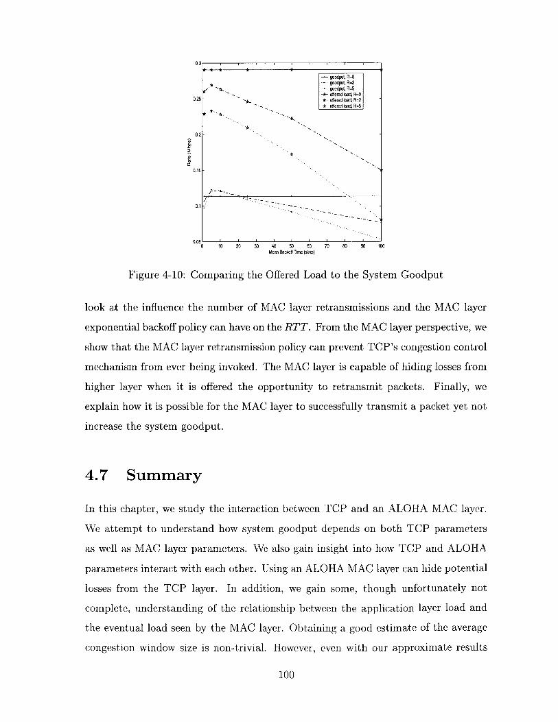
0.3
- goodput, R=0- goodput, R=2
goodput, R=5-- offered load, R=0
0.25 - ~ offered load, R=2*offered load, R=5
0.2-
0.15 -
.
0.1
0.05'0 10 20 30 40 50 60 70 80 90 100
Mean Backoff Time (d§ots)
Figure 4-10: Comparing the Offered Load to the System Goodput
look at the influence the number of MAC layer retransmissions and the MAC layer
exponential backoff policy can have on the RTT. From the MAC layer perspective, we
show that the MAC layer retransmission policy can prevent TCP's congestion control
mechanism from ever being invoked. The MAC layer is capable of hiding losses from
higher layer when it is offered the opportunity to retransmit packets. Finally, we
explain how it is possible for the MAC layer to successfully transmit a packet yet not
increase the system goodput.
4.7 Summary
In this chapter, we study the interaction between TCP and an ALOHA MAC layer.
We attempt to understand how system goodput depends on both TCP parameters
as well as MAC layer parameters. We also gain insight into how TCP and ALOHA
parameters interact with each other. Using an ALOHA MAC layer can hide potential
losses from the TCP layer. In addition, we gain some, though unfortunately not
complete, understanding of the relationship between the application layer load and
the eventual load seen by the MAC layer. Obtaining a good estimate of the average
congestion window size is non-trivial. However, even with our approximate results
100

we are able to show that TCP effectively constrains the flow of data down to the
MAC layer. By choking the flow of data to the MAC layer TCP allows us to stabilize
ALOHA.
101

102

Chapter 5
Conclusion and Future Work
In our work, we consider two separate problems. However, the fundamental issues are
the same. We seek to understand the interaction of TCP and MAC layer protocols
in the context of space and satellite communications. Though our work is relevant in
other areas, we construct our models with satellite applications in mind.
We consider both centralized and distributed models. In the centralized model, we
assume a point-to-point connection exists between ground terminals and the satellite.
The source and destination are both ground terminals. They are connected via a
satellite link that serves many other such connections. With all these connections,
the satellite trunk link can become congested. Therefore, we concern ourselves with
scheduling for bottleneck links.
In the distributed model, we consider a random access channel. As before, source
and destination ground terminals are connected via a satellite link. The difference
is that ground terminals are not allocated a specific portion of the bandwidth for
transmission. All sessions must contend for the channel. Packet delivery is not
guaranteed. If multiple sessions attempt to transmit at the same time a collision will
occur. We examine the combined performance of TCP and random access protocols.
103

5.1 Summary
We study the centralized model in depth in Chapter 2, where we focus almost exclu-
sively on the problem of queue management. We discuss specific queue management
policies in use today and their shortcomings. We then propose our own queue manage-
ment schemes, the Shortest Window First and the Smallest Sequence Number First
scheduling policy. Both schedulers are implemented in conjunction with an ALQD
policy. Our motivation in designing these policies is to provide increased fairness to
lossy and high delay sessions. We also realized that schemes which give priority to
packets from lossy and high propagation delay sessions also provide benefits to ses-
sions transmitting short files. We show that our schedulers have enhanced fairness
properties when transmitting packets from lossy or high delay sessions. We also show
that our schedulers can reduce the delay experienced by short sessions. In fact, when
the percentage of the load comprised by short sessions is small, SWF can reduce the
transmission time of short sessions while maintaining roughly the same transmission
time for long sessions as round robin.
We look at a distributed MAC layer implementation. We specifically consider a
random access ALOHA MAC layer. Sessions are not perfectly scheduled; they con-
tend for access to the same channel. If multiple sessions transmit packets at the
same time collisions will undoubtedly occur. Through simulations, we optimize the
performance of a combined ALOHA-TCP implementation. We also attempt to un-
derstand how TCP and ALOHA parameters interact with each other. Running TCP
over ALOHA, stabilizes the performance of ALOHA. In theoretical ALOHA, as load
increases, system goodput decreases. However, in simulation, as the load increases
goodput eventually stabilizes. In addition, as the number of MAC layer retrans-
missions increases so does the goodput. The MAC layer can recover from collisions
before TCP discovers packets have been lost. This prevents TCP's congestion control
algorithm from being invoked. Thus, the congestion window is not constantly closing.
104

5.2 Future Work
The study of our scheduler shows improved performance in the transmission of short
messages. We are also able to show improved fairness for isolated misbehaving (lossy
or high propagation delay) sessions. Although we are able to make substantial im-
provements in some cases, there is room for more improvement.
The primary weakness of SWF is that as file lengths increase, the advantage
provided by SWF decreases. We are interested in studying a scheduling and packet
admission policy that transmits packets based not on window size, but on the amount
of the file left to transmit. Sessions that have only a few packets left to transmit would
have their packets sorted to the front of the queue and be given priority. In order to
implement such a scheme, an additional field for the message length would need to be
created in the TCP header. The sorting metric in this case is the difference between
the message length field and the raw sequence number. When the difference is small,
packets will be moved to the front of the queue. We believe this scheduler can improve
the performance of short term file transfers in a mixed file length traffic scenario. In
addition, it would provide improved performance over FIFO with DropTail and DRR
with LQD, in the case where isolated sessions are transmitted over lossy channels
or have high RTTs. The potential problems of such a scheduler are similar to those
of SSF and pertain to the use of the sequence number. They can be addressed by
making the scheduler do a little more work as we suggested with SSF. We believe a
thorough study of such a scheduler could provide valuable insight into scheduling to
reduce latency of TCP sessions.
Our work is unique in that we looked for alternate metrics to schedule packets
and manage our queue. However, we only looked at two possible metrics. Looking
into the performance of a scheduler relying on other metrics could provide further
insight on ways to improve the performance of TCP over satellite links. In addition,
looking at different drop policies could be useful as well. Specifically, it would be
interesting to drop packets from the front of queue instead of the back of the queue.
It is possible that this could cause losses to be discovered much more rapidly. In
105

general, the understanding and refining of the drop policy is an interested problem.
Our analysis of ALOHA and TCP reaffirms our intuition. In existing literature
on TCP and random access protocols, ACKs are transmitted across random access
channels along with data packets. We also consider the case where ACKs are trans-
mitted across random access channels and explain our reasons for doing so in Chapter
4. However, transmitting ACKs across random access channels complicates our at-
tempts to understand the interaction of TCP's congestion control algorithm with that
of ALOHA. Therefore, transmitting ACKs across point-to-point links where collisions
cannot occur might provide a more complete picture of TCP and ALOHA interaction.
Our work focused exclusively on understanding TCP and ALOHA interactions
through simulations. However, another approach would be to look at their relation-
ship from a purely analytic point of view. There has been considerable analysis of
both TCP and ALOHA individually. As of yet, no work has been done in trying to
study the combined behavior of the two protocols.
106

Appendix A
Further Details on TCP
A.1 Estimating the RTT and Computing the RTO
Originally, the retransmission timeout interval was computed using the following
equations
RTTest = a -RTTest + (1 - a)RTTest (A.1)
RTO = 2RTTest (A.2)
a is used to smooth the RTT estimate. A large a leads to a more stable estimate
of the RTT. However, it makes the estimate slower to respond to change. A smaller
a is much more responsive to change. a can take values between 0 and 1.
To make TCP more responsive to packet losses, Karn and Partridge proposed
the exponential backoff scheme. Each time TCP retransmits a packet, it doubles the
length of the timeout interval. While in principle, this is the correct way to approach
the problem, it can be improved. The deviation, -, of the estimated RTT should be
considered when computing the timeout interval. This can be accomplished through
the use of the following equations
S= RTTsamp - RTTest (A.3)
RTTest = RTTest + 6 - (A.4)
107
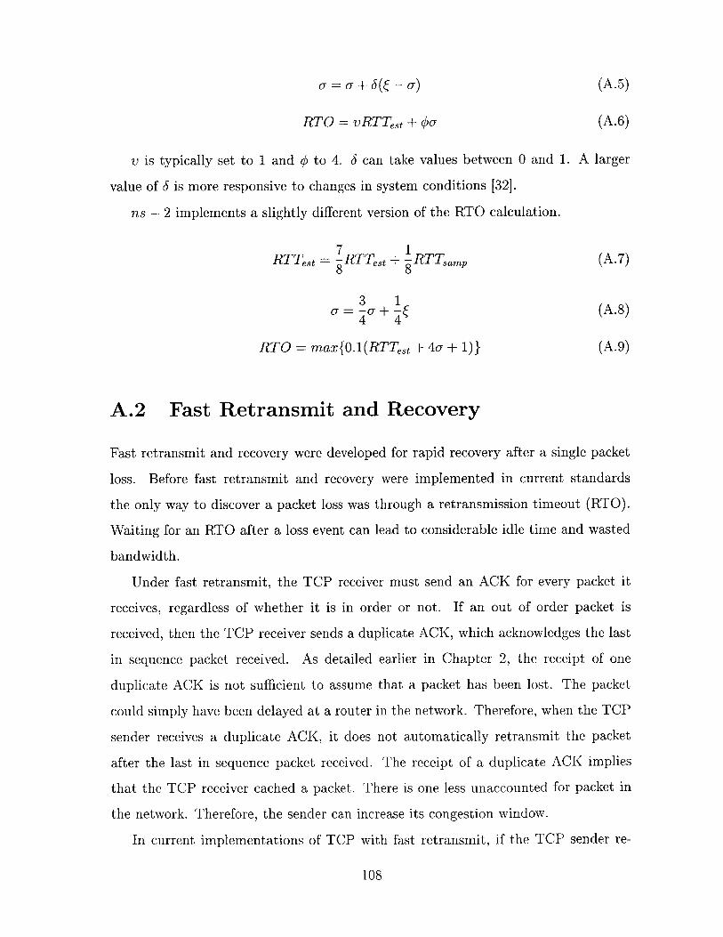
a = a + 6(-u) or)
RTO = vRTTest + 4O- (A.6)
v is typically set to 1 and # to 4. 6 can take values between 0 and 1. A larger
value of 6 is more responsive to changes in system conditions [32].
ns - 2 implements a slightly different version of the RTO calculation.
7 1RTTest = -RTTest + -RTTsamp (A-7)
8 8
3 1= + 1( (A.8)
44
RTO = max{0.1(RTTest + 4j + 1)} (A.9)
A.2 Fast Retransmit and Recovery
Fast retransmit and recovery were developed for rapid recovery after a single packet
loss. Before fast retransmit and recovery were implemented in current standards
the only way to discover a packet loss was through a retransmission timeout (RTO).
Waiting for an RTO after a loss event can lead to considerable idle time and wasted
bandwidth.
Under fast retransmit, the TCP receiver must send an ACK for every packet it
receives, regardless of whether it is in order or not. If an out of order packet is
received, then the TCP receiver sends a duplicate ACK, which acknowledges the last
in sequence packet received. As detailed earlier in Chapter 2, the receipt of one
duplicate ACK is not sufficient to assume that a packet has been lost. The packet
could simply have been delayed at a router in the network. Therefore, when the TCP
sender receives a duplicate ACK, it does not automatically retransmit the packet
after the last in sequence packet received. The receipt of a duplicate ACK implies
that the TCP receiver cached a packet. There is one less unaccounted for packet in
the network. Therefore, the sender can increase its congestion window.
In current implementations of TCP with fast retransmit, if the TCP sender re-
108
(A.5)
ceives three duplicate ACKs, it assumes that the segment following the last ACKed
packet was lost and retransmits it.
The fast retransmit and recovery algorithm are typically implemented in the fol-
lowing manner.
1. When the third duplicate ACK is received, the slow start threshold is set to one
half of the current congestion window size, but no less than 2 packets.
2. The lost packet is retransmitted. The congestion window is then set to the slow
start threshold plus 3 packets, one for each duplicate ACK received. The idea
is to inflate the congestion window by the number of packet that have left the
network and are cached at the receiver.
3. Each time an additional duplicate ACK arrives, the congestion window is incre-
mented by one packet. If the congestion window allows it, another packet can
be transmitted. The constant flow of duplicate ACKs allows TCP to continue
to send data.
4. When an ACK that acknowledges new data arrives, the congestion window is
deflated. It is set to the value of the slow start threshold. This ACK should ac-
knowledge the retransmission from step 2. It should take roughly one round trip
time from the time of the retransmission. This ACK should also acknowledge
all the packets sent between the lost packet and the first duplicate ACK.
5. Return to transmitting new packets in congestion avoidance. This is the fast
recovery portion of the algorithm. The sender does not have to close its entire
window.
Fast retransmit and recovery do not work well if multiple packets are dropped
within the same window. This is because the algorithm only retransmits the first
packet after receiving the third duplicate acknowledgment. In fast recovery, all other
packet losses are discovered through use of RTOs. If a packet loss is discovered
through an RTO, several packets may be retransmitted. However, when TCP Reno
109

fast retransmit is invoked, only one packet needs to be resent. If a retransmission is
lost, it suggests extreme congestion, and the sender has to take a timeout.
A.3 TCP New Reno [15]
The basic problem with fast retransmit is that it only allows one retransmission
without waiting for a RTO. If multiple packets from the same window are lost, the
performance of TCP Reno is not very good. The problem of recovering from multiple
losses within the same window was solved through the use of partial acknowledgments.
In the New Reno modification, additional information is available in the new
acknowledgment that arrives after the receipt of three duplicate ACKs and the re-
transmission of the lost packet. If there were multiple drops within the window, this
new ACK would acknowledge some, but not all of the data transmitted between the
lost packet and the receipt of the first new ACK. This ACK is known as a partial
ACK since it does not completely acknowledge all the available data.
The fast retransmit and recovery algorithm of New Reno is very similar to that
of TCP Reno. Steps 1 to 3 are exactly the same except in step 1, we also store the
value of the highest sequence number sent so far.
1. If an ACK that acknowledges all new data arrives, the congestion window is
deflated. It is set to the value of the slow start threshold. This ACK should
acknowledge the retransmission from step 2. It should take roughly one round
trip time from the time of the retransmission. This ACK should also acknowl-
edge all the packets sent between the lost packet and the first duplicate ACK.
The TCP sender returns to transmitting new packets in congestion avoidance.
2. If instead a partial ACK arrives, the TCP sender retransmits the first unac-
knowledged packet. It also "partially deflates" its window. The congestion
window is reduced by the number of newly acknowledged packets and incre-
mented by one packet. Fast recovery does not end. Any other duplicate ACKs
that arrive are handled according to steps steps 2 and 3.
110

A.4 TCP with Selective Acknowledgments [28]
TCP with selective acknowledgments is typically referred to as TCP SACK. It com-
bines a selective acknowledgment mechanism with a selective repeat mechanism. In
baseline TCP and Reno and New Reno variations, cumulative ACKs are used. Cu-
mulative ACKs acknowledge the highest in-sequence packet received. As such, they
cannot provide the TCP sender with much information. Through the receipt of dupli-
cate ACKs, the sender can determine that the packet following the last acknowledged
packet has been lost, but it provides no information regarding subsequent packets.
The SACK is meant to provide additional information about the state of the TCP
receiver's buffer.
Through the SACK option, the TCP receiver can inform the sender of any non-
adjacent blocks of data that have been received. The sender then retransmits the
packets that are missing from the receive buffer. The use of the SACK option can
help prevent the retransmission of redundant data. When the TCP receiver receives
a packet, it acknowledges its data in one of two ways.
1. If there are no non-contiguous blocks in the receiver's buffer, then a cumulative
ACK is sent.
2. If there are gaps remaining the receiver's buffer a SACK is sent. Each SACK
can specify up to three missing packets.
The behavior of TCP SACK with multiple losses is like that of TCP Reno with a
single loss.
111

112

Appendix B
SWF Experimentation and Results
B.1 Lossy Channels
One session with packet loss rate of 10%. Other nine sessions lossless.
Scheduler Total Goodput Goodput of Lossy Goodput of Lossless
(bps) Session (bps) Session (bps)
SWF w/ALQD 926216 31094 99458
SSF w/ALQD 947261 31331 101770
DRR w/LQD 951041 26534 102723
FIFO w/DropTail 953099 13453 104405
Five sessions with packet loss rate 10%. Other five sessions lossless.
Scheduler Total Goodput Goodput of Lossy Goodput of Lossless
(bps) Session (bps) Session (bps)
SWF w/ALQD 930050 29258 156750
SSF w/ALQD 940760 29219 158930
DRR w/LQD 949450 27262 162630
FIFO w/DropTail 951340 12858 177410
One session with packet loss rate 1%. Other nine sessions lossless.
113

Scheduler Total Goodput Goodput of Lossy Goodput of Lossless
(bps) Session (bps) Session (bps)
SWF w/ALQD 924900 94092 92312
SSF w/ALQD 959576 94766 96090
DRR w/LQD 951845 89960 95915
FIFO w/DropTail 954804 46443 100929
Five sessions with packet loss rate 1%. Other five session lossless.
Scheduler Total Goodput Goodput of Lossy Goodput of Lossless
(bps) Session (bps) Session (bps)
SWF w/ALQD 927760 97988 87560
SSF w/ALQD 949550 95087 94820
DRR w/LQD 950970 93148 97050
FIFO w/DropTail 953750 56059 134690
B.2 High RTTs
One Session with delay 75ms Delay and nine other sessions with delay 250ms.
Scheduler Total Goodput Average Goodput of Average Goodput of
(bps) Low Delay Session (bps) High Delay Session(bps)
SWF w/ ALQD 923090 119746 89260
DRR w/ LQD 952644 102039 94512
FIFO w/ DropTail 983537 518576 48329
One session with delay 1.0 seconds and nine sessions with delay 0.5 seconds.
Scheduler Total Goodput Average Goodput of Average Goodput of
(bps) High Delay Session (bps) Low Delay Session (bps)
SWF w/ALQD 925262 63057 95801
SSF w/ALQD 948893 95585 94812
DRR w/LQD 949814 84580 96137
FIFO w/DropTail 953443 14905 104282
Half of the sessions with delay 1.0 seconds and other half with delay 0.5
seconds.
114
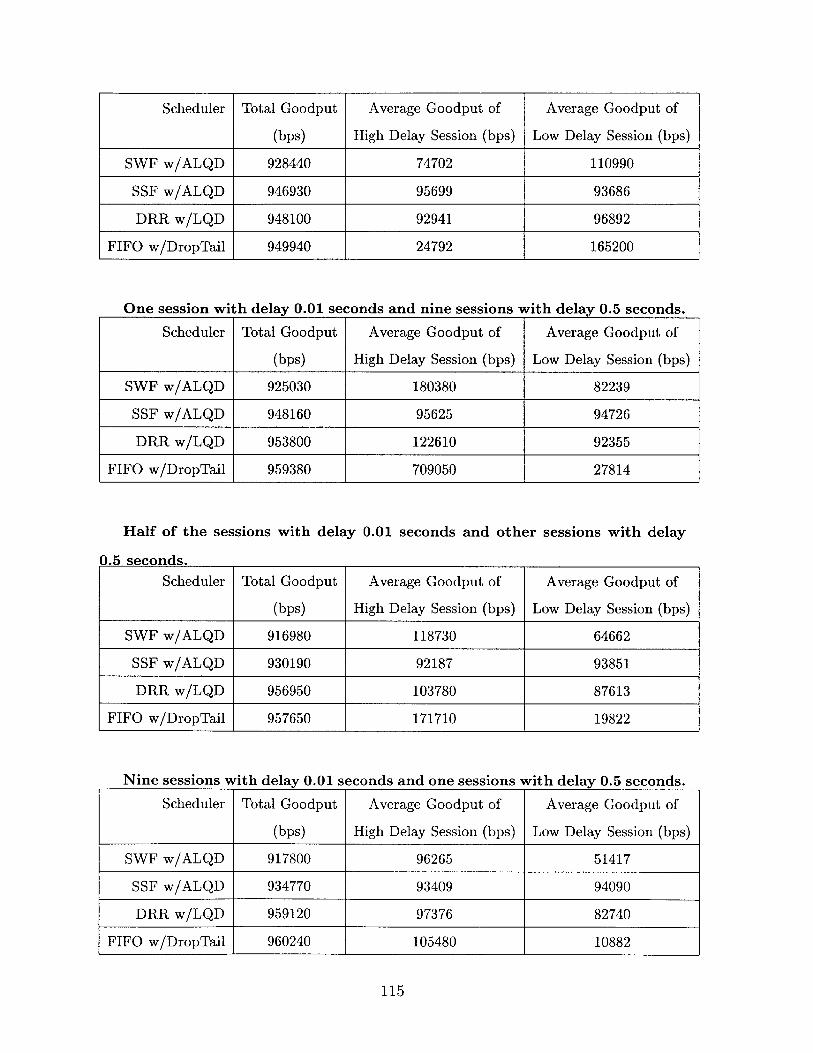
Scheduler Total Goodput Average Goodput of Average Goodput of
(bps) High Delay Session (bps) Low Delay Session (bps)
SWF w/ALQD 928440 74702 110990
SSF w/ALQD 946930 95699 93686
DRR w/LQD 948100 92941 96892
FIFO w/DropTail 949940 24792 165200
One session with delay 0.01 seconds and nine sessions with delay 0.5 seconds.
Scheduler Total Goodput Average Goodput of Average Goodput of
(bps) High Delay Session (bps) Low Delay Session (bps)
SWF w/ALQD 925030 180380 82239
SSF w/ALQD 948160 95625 94726
DRR w/LQD 953800 122610 92355
FIFO w/DropTail 959380 709050 27814
Half of the sessions with delay 0.01 seconds and other sessions with delay
0.5 seconds.
Scheduler Total Goodput Average Goodput of Average Goodput of
(bps) High Delay Session (bps) Low Delay Session (bps)
SWF w/ALQD 916980 118730 64662
SSF w/ALQD 930190 92187 93851
DRR w/LQD 956950 103780 87613
FIFO w/DropTail 957650 171710 19822
Nine sessions with delay 0.01 seconds and one sessions with delay 0.5 seconds.
Scheduler Total Goodput Average Goodput of Average Goodput of
(bps) High Delay Session (bps) Low Delay Session (bps)
SWF w/ALQD 917800 96265 51417
SSF w/ALQD 934770 93409 94090
DRR w/LQD 959120 97376 82740
FIFO w/DropTail 960240 105480 10882
115

B.3 Load Variations
10KB and 100KB mix
short files long files
%load comprised SWF SSF DRR FIFO SWF SSF DRR FIFO
by short sessions
10 1.8270 1.6723 2.5008 3.3430 17.1903 45.0722 19.5875 12.2118
20 2.3595 2.8546 19.9251 20.6455
30 2.3800 1.9996 3.0321 3.8329 18.7214 42.7498 18.7321 11.9129
40 2.7424 2.0602 3.0796 4.1750 21.1000 47.9792 20.4862 11.7690
50 3.2163 2.1130 3.2327 4.1015 23.0162 48.3900 21.6043 11.3625
60 3.3180 2.2108 3.3593 4.1312 24.4838 49.8480 21.9707 10.6747
70 3.8003 2.5398 3.5515 4.1822 30.4663 51.2028 22.7861 10.5791
1MB and 10MB mix
short files long files
%load comprised SWF SSF DRR FIFO SWF SSF DRR FIFO
by short sessions
25 55.3177 613.7636 56.8126 70.7278 391.5026 2970.7 454.7994 415.7342
37.5 49.6329 1047.3 58.4159 68.3010 354.9727 2988.0 449.0263 402.8855
50 49.6489 1293.3 61.4803 68.1609 496.4687 2683.2 489.5326 423.6173
62.5 77.9719 1811.9 74.3996 78.958 578.2845 2793.2 530.1571 508.5118
75 97.1228 2185.0 82.7453 90.6608 724.7029 2904 629.3138 572.7837
B.4 Message Size Variations
Poisson Arrivals, interarrival time 2s
116

file size (KB) SWF DRR FIFO
10 1.668 2.041 4.513
20 2.263 2.893 7.486
30 3.753 4.1454 9.009
50 7.274 7.878 13.85
75 12.731 12.987 19.501
100 18.997 19.092 26.143Standard Deviation
file size (KB) SWF DRR FIFO
10 0.6411 7.7278 266.4516
25 0.3611 6.3735 86.5545
50 1.8547 8.6787 85.7593
75 23.8368 12.2259 86.1020
100 38.5707 14.0560 108.3535
117

118

Appendix C
ALOHA Results
C.1 Goodput Results
Goodput vs. Backoff Time when system load is 0.4Mbps
# of MAC layer rtx
mean backoff (slots) 0 1 2 3 4 5
1 0.1135 0.1127 0.1076 0.1035 0.1011 0.0962
5 0.1135 0.1148 0.1186 0.1234 0.1234 0.1239
10 0.1135 0.1148 0.1199 0.1220 0.1216 0.1226
25 0.1135 0.1084 0.1113 0.1117 0.1103 0.1088
50 0.1135 0.1006 0.1004 0.0972 0.0952 0.0917
100 0.1135 0.0905 0.0750 0.0654 0.0599 0.0548
Goodput vs. Backoff Time when the system load is 0.08Mbps
# of MAC layer rtx
mean backoff (slots) 0 1 2 3 4 5
1 0.0664 0.0748 0.0781 0.0783 0.0785 0.0786
5 0.0664 0.0787 0.0788 0.0788 0.0788 0.0788
10 0.0664 0.0787 0.0788 0.0787 0.0788 0.0788
25 0.0664 0.0787 0.0786 0.0787 0.0787 0.0787
50 0.0664 0.0783 0.0783 0.0781 0.0782 0.0778
100 0.0664 0.0773 0.0752 0.0675 0.0593 0.0553
Goodput vs. Advertised Window size when the mean backoff is five slots.
119

mean backoff time is ten slots
Load per Session
# of MAC layer rtx 80Kbps 40Kbps 20Kbps 8Kbps 4Kbps
0 0.112013 0.113533 0.103869 0.066435 0.036870
1 0.119942 0.1148 0.115830 0.078714 0.039373
2 0.125168 0.1199 0.123430 0.078797 0.039379
3 0.128493 0.1220 0.126474 0.078749 0.039386
4 0.128925 0.1216 0.127293 0.078781 0.039382
5 0.129616 0.1226 0.127898 0.078784 0.039382
Goodput vs Load. The mean backoff is five slots and the advertised window
of six packets.
# of MAC layer rtx
system load 0 5
1.6Mbps 0.1153 0.1234
0.8Mbps 0.1145 0.1233
0.4Mbps 0.1153 0.1225
0.2Mbps 0.1065 0.1225
0.1Mbps 0.0781 0.0984
0.08Mbps 0.0669 0.0788
0.04Mbps 0.0363 0.0394
0.02Mbps 0.0191 0.0196
120
# of MAC layer rtx
advertised window (pkts) 0 1 2 3 4 5
1 0.0709 0.0988 0.1054 0.1061 0.1077 0.1077
2 0.0921 0.1115 0.1201 0.1209 0.1233 0.1226
4 0.1111 0.1152 0.1192 0.1227 0.1233 0.1235
6 0.1137 0.1151 0.1212 0.1227 0.1244 0.1229
10 0.1138 0.1144 0.1183 0.1236 0.1232 0.1237
25 0.1135 0.1148 0.1190 0.1234 0.1234 0.1239
50 0.1135 0.1148 0.1186 0.1234 0.1234 0.1239
75 0.1135 0.1148 0.1186 0.1234 0.1234 0.1239
100 0.1135 0.1148 0.1186 0.1234 0.1234 0.1239
Goodput vs. # of MAC layer rtx when the

Goodput vs. Number of Sessions. The mean backoff is five slots.
# of MAC layer rtx
# of sessions 0 5
5 0.1244 0.1131
10 0.1153 0.1225
20 0.1110 0.1268
30 0.1119 0.1274
40 0.1089 0.1249
50 0.1021 .1240
60 0.1015 .1230
C.2 Collision Discovery
The probability of collision when the system load is 0.4Mbps
I # of MAC layer rtx
mean backoff (slots) 0 1 2 3 4 5
1 0.1254 0.3312 0.4500 0.5349 0.5855 0.6312
5 0.1254 0.3545 0.4754 0.5429 0.5950 0.6311
10 0.1254 0.3669 0.4827 0.5533 0.5979 0.6249
25 0.1254 0.3723 0.4844 0.5469 0.5878 0.6217
50 0.1254 0.3793 0.4803 0.5350 0.5710 0.6001
100 0.1254 0.3730 0.4626 0.5137 0.5433 0.5713The probabilitv collisions are discovered through RTOs. The s
0.4Mbps
rstem load is
# of MAC layer rtx
mean backoff (slots) 0 1 2 3 4 5
1 0.6450 0.2458 0.1446 0.0997 0.0783 0.0616
5 0.6450 0.2212 0.1140 0.0702 0.0476 0.0347
10 0.6450 0.2132 0.1098 0.0656 0.0438 0.0316
25 0.6450 0.2205 0.1095 0.0651 0.0458 0.0312
50 0.6450 0.2266 0.1117 0.0681 0.0482 0.0340
100 0.6450 0.2332 0.1060 0.0641 0.0437 0.0314
Probability collisions are discovered through duplicate ACKs. The system
121
ytmlodi

load is 0.4Mbps
# of MAC layer rtx
mean backoff (slots) 0 1 2 3 4 5
1 0.2284 0.0581 0.0336 0.0224 0.0177 0.014
5 0.2284 0.0474 0.0275 0.0229 0.0193 0.0171
10 0.2284 0.0421 0.0256 0.0205 0.0191 0.0186
25 0.2284 0.0365 0.0221 0.0205 0.0188 0.0186
50 0.2284 0.0311 0.0224 0.0208 0.0200 0.0199
100 0.2284 0.0309 0.0223 0.0205 0.0227 0.0196
The probability
0.8Mbps
collisions are discovered through RTOs. The system load is
# of MAC layer rtx
mean backoff (slots) 0 1 2 3 4 5
1 0.9186 0.4626 0.2974 0.2176 0.1695 0.1374
25 0.9186 0.2503 0.1728 0.1273 0.1000 0.0814
50 0.9186 0.2655 0.1750 0.1249 0.0942 0.0736
100 0.9186 0.3827 0.2326 0.1629 0.1235 0.0968
Probability collisions are discovered through duplicate ACKs. The system
load is 0.08Mbps
# of MAC layer rtx
mean backoff (slots) 0 1 2 3 4 5
1 0.0602 0.0221 0.0123 0.0087 0.0067 0.0059
25 0.0602 0.0056 0.0069 0.0073 0.0076 0.0083
50 0.0602 0.0083 0.0091 0.0104 0.0118 0.0128
100 0.0602 0.0234 0.0188 0.0173 0.0172 0.0170
C.3 Wasted Transmissions
The probability a transmission is wasted when the system load is 0.4Mbps
122

The probability
0.4Mbps.
a successful transmission is wasted. The system load is
# of MAC layer rtx
mean backoff (slots) 0 1 2 3 4 5
1 0.0196 0.0173 0.0156 0.0143 0.0150 0.0139
5 0.0196 0.0243 0.0313 0.0302 0.0119 0.0128
10 0.0196 0.0256 0.0366 0.0201 0.0107 0.0148
25 0.0196 0.0209 0.0161 0.0148 0.0136 0.0142
50 0.0196 0.0249 0.0196 0.0183 0.0180 0.0174
100 0.0196 0.0314 0.0297 0.0285 0.0297 0.0288
C.4 Round T rip Time and Variance
Round Trip Time when the system load is 0.4Mbps.
# of MAC layer rtx
mean backoff (slots) 0 1 2 3 4 5
1 0.5315 0.6235 0.6890 0.7495 0.8134 0.869
5 0.5315 0.6515 0.7503 0.8514 0.9421 1.0339
10 0.5315 0.6700 0.7879 0.9017 0.9905 1.0928
25 0.5315 0.7101 0.8643 0.9998 1.1194 1.2381
50 0.5315 0.7627 0.9671 1.1617 1.3565 1.5153
100 0.5315 0.8443 1.1639 1.4474 1.7398 2.0613
Variance of the Round Trip Time when the system load is 0.4Mbps.
123
# of MAC layer rtx
mean backoff (slots) 0 1 2 3 4 5
1 0.1450 0.3486 0.4655 0.5492 0.6005 0.6450
5 0.1450 0.3788 0.5067 0.5730 0.6069 0.6439
10 0.1450 0.3925 0.5193 0.5734 0.6086 0.6397
25 0.1450 0.3933 0.5005 0.5617 0.6015 0.6359
50 0.1450 0.4041 0.4998 0.5533 0.5889 0.6175
100 0.1450 0.4044 0.4923 0.5422 0.5730 0.6001

# of MAC layer rtx
mean backoff (slots) 0 1 2 3 4 5
1 0.3645 0.2883 0.3227 0.3693 0.4189 0.4735
5 0.3645 0.2916 0.3499 0.4129 0.4650 0.5325
10 0.3645 0.2995 0.3730 0.4411 0.5108 0.5799
25 0.3645 0.3249 0.4349 0.5426 0.6488 0.7378
50 0.3645 0.3720 0.5352 0.7117 0.8852 1.0340
100 0.3645 0.4283 0.7177 0.9740 1.2888 1.5625
C.5 Offered Load and Traffic Shaping
Average Congestion Window Size when load is 0.4Mbps
mean backoff (slots) 0 1 2 3 4 5
1 1.9291 2.1360 2.2390 2.3569 2.4221 2.4837
5 1.9291 2.2612 2.5243 2.7046 2.8829 3.0085
10 1.9291 2.3330 2.5909 2.8096 2.9775 3.1172
25 1.9291 2.3505 2.6580 2.8971 3.1035 3.2417
50 1.9291 2.3448 2.6859 2.9528 3.1379 3.2639
100 1.9291 2.3048 2.1836 2.0850 2.1276 2.0881
Offered Load in Mbps when system load is 0.4Mbps.
# of MAC layer rtx
mean backoff (slots) 0 1 2 3 4 5
1 0.2904 0.2741 0.2600 0.2516 0.2382 0.2286
5 0.2904 0.2777 0.2692 0.2541 0.2448 0.2328
10 0.2904 0.2786 0.2631 0.2493 0.2405 0.2282
25 0.2904 0.2648 0.2460 0.2318 0.2218 0.2095
50 0.2904 0.2459 0.2222 0.2033 0.1851 0.1723
100 0.2904 0.2184 0.1501 0.1152 0.0978 0.0810
124

Bibliography
[1] M. Allman, S. Floyd, and C. Partridge. Increasing TCP's Initial Window Size.
Internet RFC 2414, 1998.
[2] M. Allman, V. Paxson, and W. Stevens. TCP Congestion Control. Internet RFC
2581, 1999.
[3] Gary Arlen. Satellite Internet still a Flightly Proposition. on-line at
http://www.washingtonpost.com/wp-dyn/articles/A43528-2002Jul9.html, 2002.
[4] A. Bakre and B.R. Badrinath. I-TCP: Indirect TCP for Mobile Hosts. In Pro-
ceedings of the 15th International Conference on Distributed Computing Systems,
1995.
[5] H. Balakrishnan, V.N. Padmanabhan, S. Seshan, and R.H. Katz. A Comparison
of Mechanisms for Improving TCP Performance over Wireless Links. IEEE/A CM
Transactions on Networking, dec 1997.
[6] Bersekas and R. Gallagher. Data Communications Networks, chapter 4. Morgan
Kaufmann, 2000.
[7] H.M. Chaskar, T.V. Lakshman, and U. Madhow. TCP over Wireless with Link
Level Error Control: Analysis and Design Methodology. A CM/IEEE Transac-
tions on Networking, 1999.
[8] D. Chiu and R. Jain. Analysis of the Increase and Decrease Algorithms for
Congestion Avoidance in Computer Networks. Computer Networks and ISDN
Systems, 1989.
125
[9] Pioneer Consulting. Abridged Executive Summary, 2002.
[10] A. Demers, S. Keshav, and S. Shenker. Analysis and Simulation of Fair Queueing
Algorithm. In Proceedings of A CM SIGCOMM, 1989.
[11] R.C. Durst, G.J. Miller, and E.J. Travis. TCP Extensions for Space Communi-
cations Protocols. In Proceedings of MOBICOM, 1996.
[12] M. Allman editor. Ongoing Research Related to TCP over Satellites. Internet
RFC 2760, 2000.
[13] W. Feng, D. Kandlur, D. Saha, and K. Shin. Blue: A New Class of Active Queue
Manegement Algorithms. Technical report, University of Michigan - Ann Arbor,
1999.
[14] W. Feng, D. Kandlur, D. Saha, and K. Shin. The Blue Queue Management
Algorithms. ACM/IEEE Transactions on Networking, 2002.
[15] S. Floyd and T. Henderson. The New Reno Modification to TCP's Fast Recovery
Algorithm. Internet RFC 2582, 1999.
[16] S. Floyd and V. Jacobson. On traffic phase effects in packet switched gateways.
Computer Communication Review, 1991.
[17] S. Floyd and V. Jacobson. Random early detection gateways for congestion
avoidance. IEEE/ACM Transactions on Networking, August 1993.
[18] M. Gerla, K. Tang, and R. Bagrodia. TCP Performance in Wireless Multi-hop
Networks. In Proceedings of IEEE WMCSA, 1999.
[19] L. Guo and I. Matta. The War Between Mice and Elephants. In Proceedings of
IEEE International Conference on Network Protocols, 2001.
[20] T. Henderson and R. Katz. Satellite Transport Protocol (STP): An SSCOP-
based Transport Protocol for Datagram Satellite Networks. In Proceedings of
2nd Workshop on Satellite Based Information Systems, 1997.
126

[21] T.R. Henderson. Networking over Next-Generation Satellite Systems. PhD thesis,
University of California Berkeley, 1999.
[22] T.R. Henderson and R.H. Katz. Transport Protocols for Internet-Compatible
Satellite Networks. IEEE Journal on Selected Areas of Communication, 1999.
[23] K.Fall and S.Floyd. Simulation-based Comparisons of Tahoe, Reno, and Sack
TCP. Computer Communications Review, 1996.
[24] T.V. Lakshman and U. Madhow. The Performance of TCP/IP for Networks with
High Bandwidth-delay Products and Random Loss. A CM/IEEE Transactions
on Networking, 1997.
[25] D. Lin and R. Morris. Dynamics of Random Early Detection. In Proceedings of
A CM SIGCOMM, 1997.
[26] C. Liu and E. Modiano. On the Interaction of Layered Protocols: the Case of
Window Flow Control and ARQ. In Proceedings of Conference on Information
Science and System, 2002.
[27] Kevin Maney. Remember those 'Iridium's going to fail' jokes? Prepare to eat
your hat. USA Today, 2003.
[28] M. Mathis, J. Madhavi, S. Floyd, and A. Romanov. TCP's Selective Acknowl-
edgement Option. Internet RFC 2018, 1996.
[29] V. Mhatre and C. Rosenberg. Performance Improvement of TCP-based Appli-
cations in a Multi-access Satellite System. In Proceedings of IEEE Vehicular
Technology Conference, 2002.
[30] R.M. Mir. Satellite Data Networks. on-line at ohio state, 2000.
[31] Yuki Noguchi. With War, Satellite Industry is Born Again. Washington Post,
2003.
[32] L.L. Peterson and B.S. Davie. Computer Networks: A Systems Approach, chap-
ter 4. Morgan Kaufmann, 2000.
127

[33] K. Poduri and K. Nichols. Simulation Studies of Increased Initial TCP Window
Size. Internet RFC 2415, 1998.
[34] M. Shreedhar and G. Varghese. Efficient Fair Queuing using Deficit Round
Robin. ACM/IEEE Transactions on Networking, 1996.
[35] F.D. Smith, F.H. Campos, K. Jeffay, and D. Ott. What TCP/IP Headers Can
Tell Us About the Internet. In Proceedings of ACM SIGMETRICS, 2001.
[36] W.R. Stevens. TCP Slow Start, Congestion Avoidance, Fast Retransmit, and
Fast Recovery Algorithms. Internet RFC 2001, 1997.
[37] B. Suter, T.V. Lakshman, D. Stiliadis, and A. Choudhury. Design Considerations
for Supporting TCP with Per-flow Queuing. In Proceedings of IEEE INFOCOM,
1998.
[38] Globalstar USA. U.S./Caribbean Annual Service Price Plans. on-line at
http://www.globalstarusa.com/pricing/coverage/pricingsheet.pdf, 2003.
[39] R. Yavatkar and N. Bhagwat. Improving End-to-End Performance of TCP over
Mobile Internetworks. In Proceedings of Mobile 94 Workshop on Mobile Com-
puting Systems and Applications, 1994.
128