energy dissipation of steel-polymer composite beam … · energy dissipation of steel-polymer...

Energy dissipation of steel-polymer composite beam-column connector

Yun-Che Wang*1, Chih-Chin Ko1

1 Department of Civil Engineering, National Cheng Kung University, Tainan 70101, Taiwan

* [email protected]

ABSTRACT

The connection between a column and a beam is of particular importance to ensure the safety of civil engineering structures, such as high-rise building and bridges. While the connector must bear sufficient force for load transmission, increase of its ductility, toughness and damping may greatly enhance the overall safety of the structures. In this work, composite beam-column connector is proposed and analyzed with the finite element method, including effects of elasticity, linear viscoelasticity, plasticity, as well as geometric nonlinearity. The composite connector consists of three parts, (1) soft steel, (2) polymer, and (3) conventional steel to be connected to beam and column. It is found that in the linear range of deformation, the energy dissipation of the composite connector is largely enhanced to the inclusion of polymer material. Since the soft steel exhibits low yield stress and high ductility, hence under large deformation the soft steel may easily be plastic deformed to gives rise to unique energy dissipation. With suitable geometric design, the connector may be tuned to exhibit different strengths and energy dissipation capabilities for real-world applications.

Keywords: Beam-column connector; soft steel; polymer; composite material; energy dissipation

1. INTRODUCTION

High damping and high stiffness materials are crucial in energy dissipation applications (Lakes, 2009). In civil engineering, one of important failure modes in steel structures is caused by the failure of the beam-column connector. Hence, the

Note: Copied from the manuscript submitted to “Steel and Composite Structures, An International Journal” for presentation at ASEM13 Congress

2063

connection between a column and beam is of particular importance to ensure the safety of civil engineering structures, such as high-rise buildings and bridges (Higashino and Okamoto 2006, Kappos 2012, Zhang and Wang 2012). The role of the connector is to transmit loading from the beam to the column, and then through the columns to the foundation of the structure. Conventional methods to connect the beam and column use bolts or welding techniques (Calado et al. 2013). These methods may give rise to enough rigidity to the connector, and hence it can sustain the large loading. However, at the same time, bolts and welds make the connector brittle, and the brittleness reduces the energy dissipation of the connector in the steel structures.

In the literature, Chen et al. (1996) proposed a cross-section area reduction method

to enhance the ductility of the beam-column connector. The ductile connectors may localize failure to the beams, and protect the columns. While the connector must bear sufficient force for load transmission, increase of its ductility, toughness and damping may greatly enhance the overall safety of the structure. Yet, current popular designs, such as the cross-section area reduction method, may have limited benefits, in terms of ductility and toughness, to the overall behavior of the beam-column system. Similar design concepts have been realized in creating energy-absorbing devices (Kelly et al. 1972, Whittaker et al. 1991, Tsai et al. 1993). All these ideas and devices do not take the advantages of composite materials with a high-damping phase.

In addition to structure-like damper devices or mass damper devices, several novel

dampers have been proposed. In the case of using viscous fluids, compound lead extrusion magnetorheological (CLEMR) dampers have recently been studied for their high energy dissipation properties (Xu et al. 2012, Zhang and Xu 2012). In addition, effective damping can be largely enhanced by using negative stiffness elements (Dong and Lakes 2012). Both of the types of the dampers require additional design considerations for real-world applications, in terms of stability and operational frequency ranges.

Composites comprising polymers and metallic materials are widely used in damping

applications. Typically, constrained layer dampers have been shown to be an effective method to obtain high damping and sufficient stiffness (Ross et al. 1959, Nashif et al. 1985, Ferreira et al. 2013). The basic idea is to combine high loss material as one phase with high stiffness material with as the other phase. The two phase viscoelastic composites have been shown to exhibit desired combination of stiffness and energy dissipation properties.

In this work, a composite connector is composed of three parts, (1) soft steel, (2)

polymer material, such as rubber, and (3) conventional steel frame, and analyzed with finite element analysis. The soft steel is defined as the steel with low yield strength and high ductility. The connector, then, is bolted or welded to the column and beam. Various designs for the composite beam-column connector are conducted and compared. In the finite element analysis, effects of geometric nonlinearity, plasticity and linear viscoelasticity are included.

2064

(a) (b)

Figure 1. Schematics of the connector (a) without polymer, and (b) with polymer (orange color).

2. CONTINUUM MODELS

In this section, first the elasticity model is described in Section 2.1, followed by the viscoelasticity mode, and finally the plasticity model. All these continuum models are adopted in the finite element numerical analysis to study the mechanical behavior of the composite beam-column connector, as it is a block of material.

2.1 Elasticity analysis

Force balance equation used in elasticity is shown in Eq. (1), where density is denoted by , time t, displacement fields 　 u, stress tensor and specific body force 　 F. The symbol 　 indicates partial derivative. Tensorial notations are not adopted for clearly presentation of the equations.

2 u

t2 F , (1)

Constitutive relationships are shown in Eq. (2) with total strain denoted by and 　inelastic strain by 　inel. The colon symbol : denotes the tensorial contraction operation between fourth-order elastic constant tensor C and second-order strain tensor.

2065

C : inel , (2)

The strain tensor follows the following geometrical relationship with the displacement fields. The gradient operator is denoted by an upper side down triangle. A superscript T indicates a tensor transpose operation.

1

2u T

u

, (3)

Combination of the all the above equations with suitable and initial boundary conditions results in the well-defined mathematical system for the elasticity problems.

2.2 Viscoelasticity analysis

When materials are viscoelastic, the force balance still obeys Eq. (1), but the constitutive relationships must be modified to reflect the nature of time dependence. The standard linear solid model is adopted, as follows.

Tr K inel I 2G 1

3Tr

0 I

2Gq, (4)

Here the bulk modulus is K, shear modulus G. The symbol Tr denotes the tensorial trace operator to sum up the diagonal terms, and second order identity tensor is denoted as I. The time dependence is embedded in the internal variable q in the above equation, and its evolution is governed by

q

t

1

q

t

1

3Tr

0 I

, (5)

The relaxation time constant is a material parameter. The standard linear solid 　requires three parameters, bulk modulus K, shear modulus G and the time constant . 　In our analysis, we provide Young’s modulus E, and the bulk modulus can be calculated from the following equation.

K EG

3 3G E . (6)

The above relationship is only valid for isotropic materials. In our analysis, each constituent, such as soft steel or polymer, is treated as isotropic materials.

2.3 Plasticity analysis

When materials are deformed into their plastic range, the associated flow rule is adopted in the present analysis, and the strain rate is determined from the yield function as follows.

2066

p F

, (7)

where the von Mises type yield function is defined by

F mises

ys

. (8)

The parameter is calculated from the yield function differentiated by stress　 (Lubliner, 1990). The yield strength evolves with deformation as follows.

ys

ys0

h, (9)

The initial yield strength 　ys0 = 130 MPa, and the hardening function 　h = 200 MPa is assumed to be independent of strain, which is commonly used in modeling steel. For standard plasticity calculations, the isotropic hardening rule is applied, i.e. for Figures 4, 5 and 6, as well as Tables 2 and 3 . For comparisons, Kinematic hardening, with a tangent modulus of 2 GPa, is considered in quasi-static loading cases, as shown in Figures 7 and 8. In addition, the elastic-perfectly plastic model is also adopted to compare the different effects on the plasticity model choice.

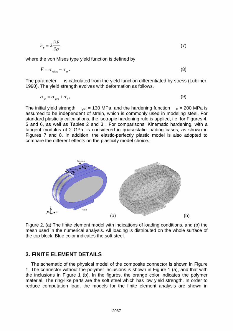
(a) (b)

Figure 2. (a) The finite element model with indications of loading conditions, and (b) the mesh used in the numerical analysis. All loading is distributed on the whole surface of the top block. Blue color indicates the soft steel.

3. FINITE ELEMENT DETAILS

The schematic of the physical model of the composite connector is shown in Figure 1. The connector without the polymer inclusions is shown in Figure 1 (a), and that with the inclusions in Figure 1 (b). In the figures, the orange color indicates the polymer material. The ring-like parts are the soft steel which has low yield strength. In order to reduce computation load, the models for the finite element analysis are shown in

2067

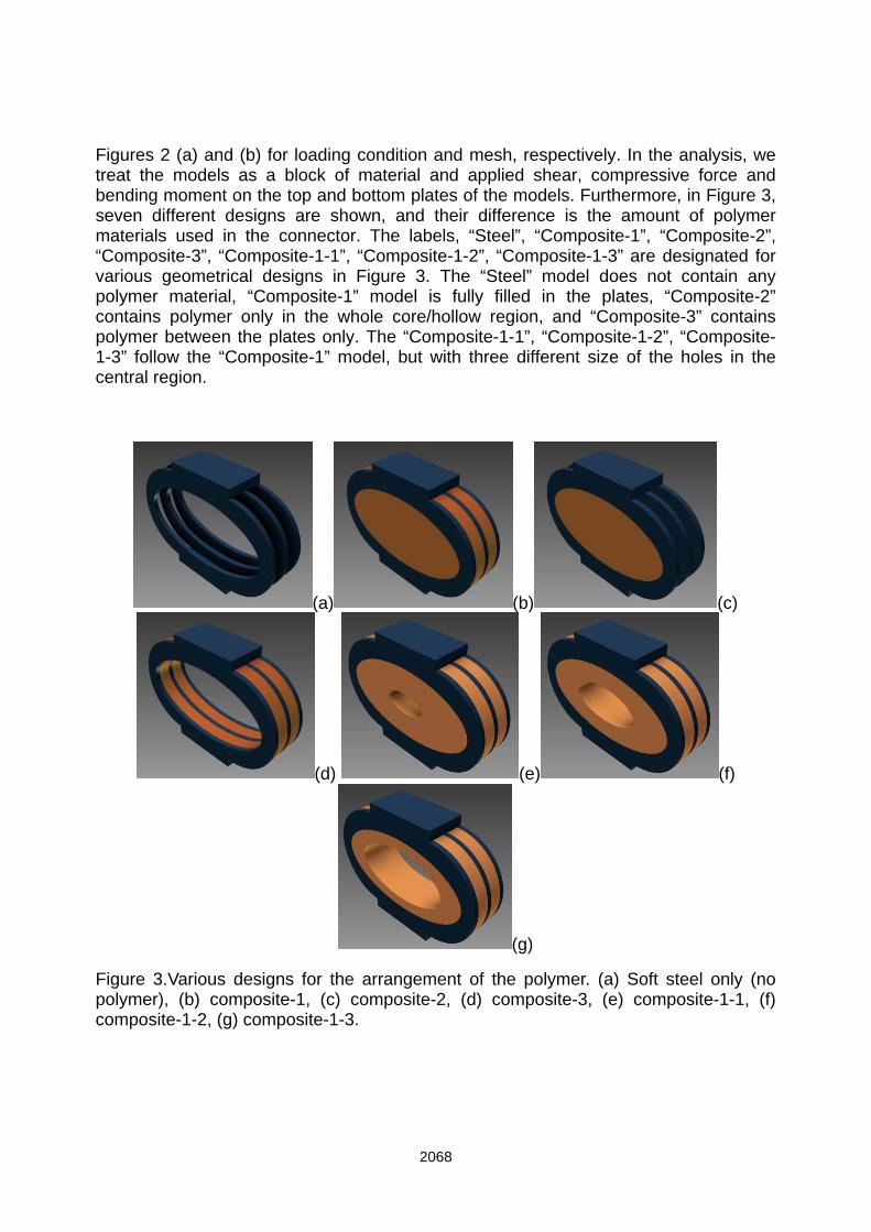
Figures 2 (a) and (b) for loading condition and mesh, respectively. In the analysis, we treat the models as a block of material and applied shear, compressive force and bending moment on the top and bottom plates of the models. Furthermore, in Figure 3, seven different designs are shown, and their difference is the amount of polymer materials used in the connector. The labels, “Steel”, “Composite-1”, “Composite-2”, “Composite-3”, “Composite-1-1”, “Composite-1-2”, “Composite-1-3” are designated for various geometrical designs in Figure 3. The “Steel” model does not contain any polymer material, “Composite-1” model is fully filled in the plates, “Composite-2” contains polymer only in the whole core/hollow region, and “Composite-3” contains polymer between the plates only. The “Composite-1-1”, “Composite-1-2”, “Composite-1-3” follow the “Composite-1” model, but with three different size of the holes in the central region.

(a) (b) (c)

(d) (e) (f)

(g)

Figure 3.Various designs for the arrangement of the polymer. (a) Soft steel only (no polymer), (b) composite-1, (c) composite-2, (d) composite-3, (e) composite-1-1, (f) composite-1-2, (g) composite-1-3.

2068

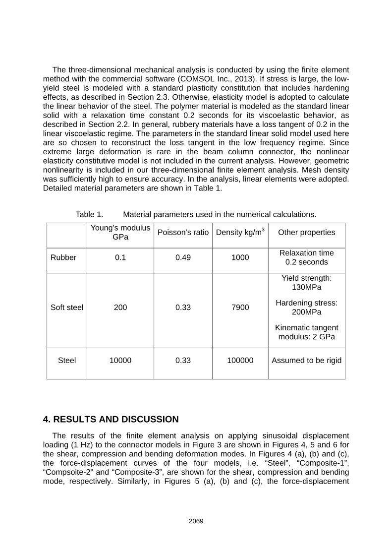
The three-dimensional mechanical analysis is conducted by using the finite element method with the commercial software (COMSOL Inc., 2013). If stress is large, the low-yield steel is modeled with a standard plasticity constitution that includes hardening effects, as described in Section 2.3. Otherwise, elasticity model is adopted to calculate the linear behavior of the steel. The polymer material is modeled as the standard linear solid with a relaxation time constant 0.2 seconds for its viscoelastic behavior, as described in Section 2.2. In general, rubbery materials have a loss tangent of 0.2 in the linear viscoelastic regime. The parameters in the standard linear solid model used here are so chosen to reconstruct the loss tangent in the low frequency regime. Since extreme large deformation is rare in the beam column connector, the nonlinear elasticity constitutive model is not included in the current analysis. However, geometric nonlinearity is included in our three-dimensional finite element analysis. Mesh density was sufficiently high to ensure accuracy. In the analysis, linear elements were adopted. Detailed material parameters are shown in Table 1.

Table 1. Material parameters used in the numerical calculations.

Young’s modulus

GPa Poisson’s ratio Density kg/m3 Other properties

Rubber 0.1 0.49 1000 Relaxation time

0.2 seconds

Soft steel 200 0.33 7900

Yield strength: 130MPa

Hardening stress: 200MPa

Kinematic tangent modulus: 2 GPa

Steel 10000 0.33 100000 Assumed to be rigid

4. RESULTS AND DISCUSSION

The results of the finite element analysis on applying sinusoidal displacement loading (1 Hz) to the connector models in Figure 3 are shown in Figures 4, 5 and 6 for the shear, compression and bending deformation modes. In Figures 4 (a), (b) and (c), the force-displacement curves of the four models, i.e. “Steel”, “Composite-1”, “Compsoite-2” and “Composite-3”, are shown for the shear, compression and bending mode, respectively. Similarly, in Figures 5 (a), (b) and (c), the force-displacement

2069

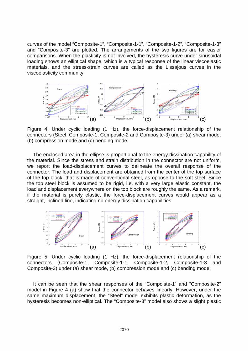
curves of the model “Composite-1”, “Composite-1-1”, “Composite-1-2”, “Composite-1-3” and “Composite-3” are plotted. The arrangements of the two figures are for easier comparisons. When the plasticity is not involved, the hysteresis curve under sinusoidal loading shows an elliptical shape, which is a typical response of the linear viscoelastic materials, and the stress-strain curves are called as the Lissajous curves in the viscoelasticity community.

(a) (b) (c)

Figure 4. Under cyclic loading (1 Hz), the force-displacement relationship of the connectors (Steel, Composite-1, Composite-2 and Composite-3) under (a) shear mode, (b) compression mode and (c) bending mode.

The enclosed area in the ellipse is proportional to the energy dissipation capability of

the material. Since the stress and strain distribution in the connector are not uniform, we report the load-displacement curves to delineate the overall response of the connector. The load and displacement are obtained from the center of the top surface of the top block, that is made of conventional steel, as oppose to the soft steel. Since the top steel block is assumed to be rigid, i.e. with a very large elastic constant, the load and displacement everywhere on the top block are roughly the same. As a remark, if the material is purely elastic, the force-displacement curves would appear as a straight, inclined line, indicating no energy dissipation capabilities.

(a) (b) (c)

Figure 5. Under cyclic loading (1 Hz), the force-displacement relationship of the connectors (Composite-1, Composite-1-1, Composite-1-2, Composite-1-3 and Composite-3) under (a) shear mode, (b) compression mode and (c) bending mode.

It can be seen that the shear responses of the “Compoiste-1” and “Composite-2”

model in Figure 4 (a) show that the connector behaves linearly. However, under the same maximum displacement, the “Steel” model exhibits plastic deformation, as the hysteresis becomes non-elliptical. The “Composite-3” model also shows a slight plastic

-40

-30

-20

-10

0

10

20

30

40

-10 -5 0 5 10

SteelComposite-1Composite-2Composite-3

For

ce, k

N

Displacement, mm

Shear

-150

-100

-50

0

50

100

150

-2 -1 0 1 2


Compression

For

ce,

kN

Displacement, mm

-6

-4

-2

0

2

4

6

-2 -1 0 1 2


Bending

For

ce,

kN

Displacement, mm

-40

-30

-20

-10

0

10

20

30

40

-15 -10 -5 0 5 10 15

Composite-1Composite-1-1Composite-1-2Composite-1-3Composite-3

For

ce, k

N

Displacement, mm

Shear

-150

-100

-50

0

50

100

150

-3 -2 -1 0 1 2 3


Compression

Displacement, mm

For

ce,

kN

-6

-4

-2

0

2

4

6

-3 -2 -1 0 1 2 3


Displacement, mm

For

ce, k

N

Bending

2070

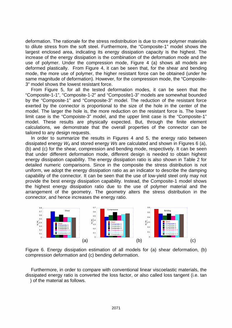
deformation. The rationale for the stress redistribution is due to more polymer materials to dilute stress from the soft steel. Furthermore, the “Composite-1” model shows the largest enclosed area, indicating its energy dissipation capacity is the highest. The increase of the energy dissipation is the combination of the deformation mode and the use of polymer. Under the compression mode, Figure 4 (a) shows all models are deformed plastically. From Figure 4, it can be seen that, for the shear and bending mode, the more use of polymer, the higher resistant force can be obtained (under he same magnitude of deformation). However, for the compression mode, the “Composite-3” model shows the lowest resistant force.

From Figure 5, for all the tested deformation modes, it can be seen that the “Composite-1-1”, “Composite-1-2” and “Composite1-3” models are somewhat bounded by the “Composite-1” and “Composite-3” model. The reduction of the resistant force exerted by the connector is proportional to the size of the hole in the center of the model. The larger the hole is, the more reduction on the resistant force is. The lower limit case is the “Compoiste-3” model, and the upper limit case is the “Composite-1” model. These results are physically expected. But, through the finite element calculations, we demonstrate that the overall properties of the connector can be tailored to any design requests.

In order to summarize the results in Figures 4 and 5, the energy ratio between dissipated energy Wd and stored energy Ws are calculated and shown in Figures 6 (a), (b) and (c) for the shear, compression and bending mode, respectively. It can be seen that under different deformation mode, different design is needed to obtain highest energy dissipation capability. The energy dissipation ratio is also shown in Table 2 for detailed numeric comparisons. Since in the composite the stress distribution is not uniform, we adopt the energy dissipation ratio as an indicator to describe the damping capability of the connector. It can be seen that the use of low-yield steel only may not provide the best energy dissipation capability. Instead, the Composite-1 model shows the highest energy dissipation ratio due to the use of polymer material and the arrangement of the geometry. The geometry alters the stress distribution in the connector, and hence increases the energy ratio.

(a) (b) (c)

Figure 6. Energy dissipation estimation of all models for (a) shear deformation, (b) compression deformation and (c) bending deformation.

Furthermore, in order to compare with conventional linear viscoelastic materials, the

dissipated energy ratio is converted the loss factor, or also called loss tangent (i.e. tan ) of the material as follows. 　

0

0.1

0.2

0.3

0.4

0.5

0.6

0.7

0.8

SteelComposite-1Composite-2Composite-3Composite-1-1Composite-1-2Composite-1-3

Wd/W

s

Shear

0

0.1

0.2

0.3

0.4

0.5

0.6

0.7


Wd/W

s

Compressive

0

0.1

0.2

0.3

0.4

0.5

0.6


Wd/W

s

Bending

2071

Wd

Ws

2

tan . (10)

The converted loss tangent is shown in Table 3 for all models. We remark that since some of the models are deformed plastically. The conversion represents an overall estimation of the loss tangent as if the material were a linear viscoelastic type. In the connector, energy dissipation may be achieved by polymer’s viscoelasticity, as well as plastic deformation of the soft steel. Under compression, the force-displacement curves of the all models are shown in Figure 4 (b) and Figure 5 (b). In this loading condition, the low-yield steel only model shows the highest energy dissipation ratio, as summarized in Figure 6 (b). Since the significant bent in the force-displacement curves, the low-yield steel is plastically deformed for the steel only model. Under this loading, adding polymer materials would reduce the stress in the steel, and hence the energy ratio is smaller. However, for shear mode, the “Steel” model shows the lowest energy dissipation.

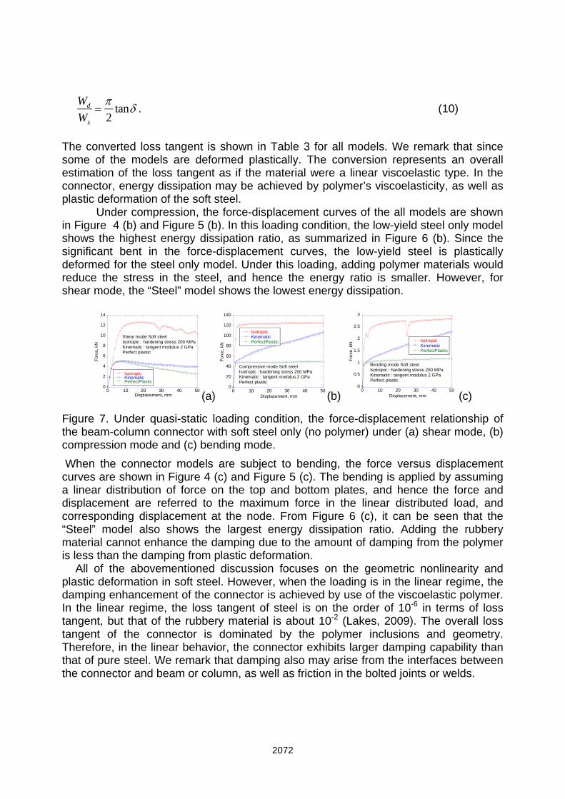
(a) (b) (c)

Figure 7. Under quasi-static loading condition, the force-displacement relationship of the beam-column connector with soft steel only (no polymer) under (a) shear mode, (b) compression mode and (c) bending mode.

When the connector models are subject to bending, the force versus displacement curves are shown in Figure 4 (c) and Figure 5 (c). The bending is applied by assuming a linear distribution of force on the top and bottom plates, and hence the force and displacement are referred to the maximum force in the linear distributed load, and corresponding displacement at the node. From Figure 6 (c), it can be seen that the “Steel” model also shows the largest energy dissipation ratio. Adding the rubbery material cannot enhance the damping due to the amount of damping from the polymer is less than the damping from plastic deformation.

All of the abovementioned discussion focuses on the geometric nonlinearity and plastic deformation in soft steel. However, when the loading is in the linear regime, the damping enhancement of the connector is achieved by use of the viscoelastic polymer. In the linear regime, the loss tangent of steel is on the order of 10-6 in terms of loss tangent, but that of the rubbery material is about 10-2 (Lakes, 2009). The overall loss tangent of the connector is dominated by the polymer inclusions and geometry. Therefore, in the linear behavior, the connector exhibits larger damping capability than that of pure steel. We remark that damping also may arise from the interfaces between the connector and beam or column, as well as friction in the bolted joints or welds.

0

2

4

6

8

10

12

14

0 10 20 30 40 50

IsotropicKinematicPerfectPlastic

For

ce, k

N

Displacement, mm

Shear mode Soft steelIsotropic : hardening stress 200 MPaKinematic : tangent modulus 2 GPaPerfect plastic

0

20

40

60

80

100

120

140

0 10 20 30 40 50


For

ce, k

N

Displacement, mm

Compressive mode Soft steelIsotropic : hardening stress 200 MPaKinematic : tangent modulus 2 GPaPerfect plastic

0

0.5

1

1.5

2

2.5

3

0 10 20 30 40 50


Bending mode Soft steelIsotropic : hardening stress 200 MPaKinematic : tangent modulus 2 GPaPerfect plastic

For

ce, k

N

Displacement, mm

2072

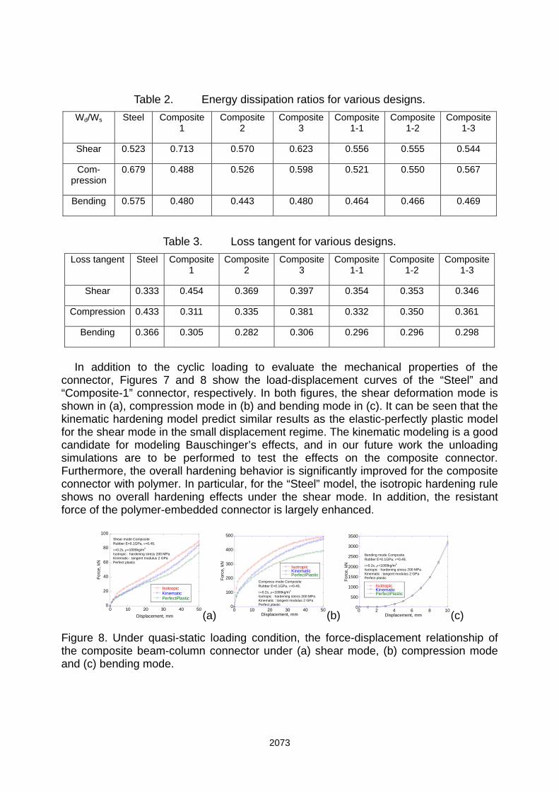
Table 2. Energy dissipation ratios for various designs.

Wd/Ws Steel Composite 1

Composite2

Composite3

Composite 1-1

Composite 1-2

Composite 1-3

Shear 0.523 0.713 0.570 0.623 0.556 0.555 0.544

Com-pression

0.679 0.488 0.526 0.598 0.521 0.550 0.567

Bending 0.575 0.480 0.443 0.480 0.464 0.466 0.469

Table 3. Loss tangent for various designs.

Loss tangent Steel Composite 1

Composite2

Composite3

Composite 1-1

Composite 1-2

Composite 1-3

Shear 0.333 0.454 0.369 0.397 0.354 0.353 0.346

Compression 0.433 0.311 0.335 0.381 0.332 0.350 0.361

Bending 0.366 0.305 0.282 0.306 0.296 0.296 0.298

In addition to the cyclic loading to evaluate the mechanical properties of the

connector, Figures 7 and 8 show the load-displacement curves of the “Steel” and “Composite-1” connector, respectively. In both figures, the shear deformation mode is shown in (a), compression mode in (b) and bending mode in (c). It can be seen that the kinematic hardening model predict similar results as the elastic-perfectly plastic model for the shear mode in the small displacement regime. The kinematic modeling is a good candidate for modeling Bauschinger’s effects, and in our future work the unloading simulations are to be performed to test the effects on the composite connector. Furthermore, the overall hardening behavior is significantly improved for the composite connector with polymer. In particular, for the “Steel” model, the isotropic hardening rule shows no overall hardening effects under the shear mode. In addition, the resistant force of the polymer-embedded connector is largely enhanced.

(a) (b) (c)

Figure 8. Under quasi-static loading condition, the force-displacement relationship of the composite beam-column connector under (a) shear mode, (b) compression mode and (c) bending mode.

0

20

40

60

80

100

0 10 20 30 40 50


Fo

rce,

kN

Displacement, mm

Shear mode CompositeRubber E=0.1GPa, =0.49,

=0.2s, =1000kg/m3

Isotropic : hardening stress 200 MPaKinematic : tangent modulus 2 GPaPerfect plastic

0

100

200

300

400

500

0 10 20 30 40 50


Compress mode CompositeRubber E=0.1GPa, =0.49,

=0.2s, =1000kg/m3


For

ce,

kN

Displacement, mm

0

500

1000

1500

2000

2500

3000

3500

0 2 4 6 8 10


For

ce, k

N

Displacement, mm

Bending mode CompositeRubber E=0.1GPa, =0.49,

=0.2s, =1000kg/m3


2073

It is known that the area underneath the quasi-static stress-strain curve is called uniaxial toughness of the material, a combinatory measure of the strength and ductility of the material. Since, in the current computer simulations, the fracture of the connectors cannot be modeled, the end points of the force-displacement curves cannot be determined by calculations. However, the two figures serve a purpose to delineate the plastic behavior of the connector with three plasticity models, i.e. the isotropic hardening model, kinematic hardening model and elastic-perfectly plastic model. It is emphasized that the isotropic hardening model is adopted in the results shown in the Figures 4, 5 and 6.

5. CONCLUSIONS

The energy dissipation capability of the composite beam-column connector studied as a material block here is largely enhanced due to several mechanisms, as follows. In the linear regime, the viscoelastic properties of polymer material increases the overall dissipation energy ratio of the composite connector about three orders of magnitudes, when compared to purely elastic properties of the steel. In the plastically deformed regime, the soft steel provides energy dissipation through plastic deformation in the expense of permanent deformation. The amount of energy dissipation depends on deformation modes, and inn the bending and compression mode, polymer materials do not enhance overall damping properties of the composite beam-column connect. However, in the shear mode, suitable choice of rubber material in its geometry may increase the energy dissipation more than have the soft steel only. In the quasi-static loading condition, the soft steel only model does not show strong overall plastic hardening with the isotropic hardening rule, while the composite connector exhibits distinctive overall hardening behavior. Finally, in reality, additional energy dissipation may arise from friction damping due to the bolt or weld connections between the connector and its neighbors.

ACKNOWLEDGEMENTS

This research work was supported by the National Science Council of the Republic of China under Grant NSC 101-2221-E-006 -206.

REFERENCES

Calado, L., Proenca, J.M., Espinha, M. and Castiglioni, C.A. (2013), “Hysteretic behavior of dissipative welded fuses for earthquake resistant composite steel and concrete frames,” Steel & Composite Structures, An International Journal, 14, 547-569.

2074

Chen, S.J., Yeh, C.H. and Chu, J.M. (1996), “Ductile steel beam-to-column connections for seismic resistance,” ASCE Journal of Structural Engineering, 122, 1292-1299.

COMSOL Inc. (2013), website: http://www.comsol.com. Dong, L. and Lakes, R.S. (2012), “Advanced damper with negative structural

stiffness elements,” Smart Materials and Structures, 21, 075026. Ferreira, A.J.M, Araujo, A.L., Neves, A.M.A., Rodrigues, J.D., Carrera, E., Cinefra,

M., Soares, C.M.M. (2013), “A finite element model using a unified formulation for the analysis of viscoelastic sandwich laminates,” Composites: Part B, 45, 1258-1264.

Higashino, M. and Okamoto, S. (2006), Response control and seismic isolation of buildings, Taylor & Francis, New York, NY, USA.

Kappos, A.J., Saiidi, M.S., Aydinoglu, M.N. and Isakovic, T. (2012), Seismic design and assessment of bridges, Springer, Dordrecht, The Netherlands.

Kelly, J.M., Skinner, R.I. and Heine, A.J. (1972), “Mechanisms of energy absorption in special devices for use in earthquake resistant structures,” National Society for Earthquake Engineering, 5, 63-88.

Lakes, R.S. (2009), Viscoelastic Materials, Cambridge University Press, New York, NY, USA.

Lubliner, J. (1990), Plasticity Theory, Macmillan Publishing Company, New York, NY, USA.

Nashif, A.D., Jones, D.I.G. and Henderson, J.P. (1985), Vibration Damping, John Wiley, New York, NY, USA.

Ross, D., Ungar, E.E., Kerwin, E.M. Jr. (1959), “Damping of plate flexural vibrations by means of viscoelastic laminate,” In ASME (Ed.), Structural Damping, pp. 49-88, New York, NY, USA.

Tsai, K.C., Chen, H.W., Hong, C.P. and Su, Y.F. (1993), “Design of steel triangular plate energy absorbers for seismic-resistant construction,” Earthquake Spectra, 9, 505-528.

Whittaker, A.S., Bertero, V.V., Thompson, C.I. and Alonso, L.J. (1991), “Seismic Testing of Steel Plate Energy Dissipation Devices,” Earthquake Spectra, 7, 563-604.

Xu, Z.D., Jia, D.H., Zhang, X.C. (2012), “Performance tests and mathematical model considering magnetic saturation for magnetorheological damper,” Journal of Intelligent Material Systems and Structures, 23, 1331-1349.

Zhang, H.D. and Wang Y.F. (2012), “Energy-based numerical evaluation for seismic performance of a high-rise steel building,” Steel & Composite Structures, An International Journal, 14, 547-569.

Zhang, X.C., Xu, Z.D. (2012), “Testing and modeling of a CLEMR damper and its application in structural vibration reduction,” Nonlinear Dynamics, 70, 1575-1588.

2075

energy dissipation of steel-polymer composite beam … · energy dissipation of steel-polymer...

Documents