energy dissipation in microfluidic beam resonators

Energy dissipation in microfluidic beam resonators

Citation SADER, JOHN E., THOMAS P. BURG, and SCOTT R.MANALIS. “Energy Dissipation in Microfluidic Beam Resonators.”Journal of Fluid Mechanics 650 (2010) : 215-250. © 2010Cambridge University Press

As Published http://dx.doi.org/10.1017/S0022112009993521

Publisher Cambridge University Press

Version Final published version

Accessed Sat Jan 12 18:58:41 EST 2019

Citable Link http://hdl.handle.net/1721.1/62854

Terms of Use Article is made available in accordance with the publisher's policyand may be subject to US copyright law. Please refer to thepublisher's site for terms of use.

Detailed Terms

The MIT Faculty has made this article openly available. Please sharehow this access benefits you. Your story matters.

http://dx.doi.org/10.1017/S0022112009993521

http://hdl.handle.net/1721.1/62854

http://libraries.mit.edu/forms/dspace-oa-articles.html

J. Fluid Mech., page 1 of 36 c© Cambridge University Press 2010

doi:10.1017/S0022112009993521

1

Energy dissipation in microfluidicbeam resonators

JOHN E. SADER1†, THOMAS P. BURG2,3

AND SCOTT R. MANALIS2,4

1Department of Mathematics and Statistics, The University of Melbourne,Victoria 3010, Australia

2Department of Biological Engineering, Massachusetts Institute of Technology,Cambridge, MA 02139, USA

3Max Planck Institute for Biophysical Chemistry, 37077 Goettingen, Germany4Department of Mechanical Engineering, Massachusetts Institute of Technology,

Cambridge, MA 02139, USA

(Received 18 May 2009; revised 16 November 2009; accepted 17 November 2009)

The fluid–structure interaction of resonating microcantilevers immersed in fluid hasbeen widely studied and is a cornerstone in nanomechanical sensor development. Inmany applications, fluid damping imposes severe limitations by strongly degradingthe signal-to-noise ratio of measurements. Recently, Burg et al. (Nature, vol. 446,2007, pp. 1066–1069) proposed an alternative type of microcantilever device wherebya microfluidic channel was embedded inside the cantilever with vacuum outside.Remarkably, it was observed that energy dissipation in these systems was almostidentical when air or liquid was passed through the channel and was 4 ordersof magnitude lower than that in conventional microcantilever systems. Here, westudy the fluid dynamics of these devices and present a rigorous theoretical modelcorroborated by experimental measurements to explain these observations. In sodoing, we elucidate the dominant physical mechanisms giving rise to the uniquefeatures of these devices. Significantly, it is found that energy dissipation is not amonotonic function of fluid viscosity, but exhibits oscillatory behaviour, as fluidviscosity is increased/decreased. In the regime of low viscosity, inertia dominatesthe fluid motion inside the cantilever, resulting in thin viscous boundary layers –this leads to an increase in energy dissipation with increasing viscosity. In the high-viscosity regime, the boundary layers on all surfaces merge, leading to a decreasein dissipation with increasing viscosity. Effects of fluid compressibility also becomesignificant in this latter regime and lead to rich flow behaviour. A direct consequenceof these findings is that miniaturization does not necessarily result in degradation inthe quality factor, which may indeed be enhanced. This highly desirable feature isunprecedented in current nanomechanical devices and permits direct miniaturizationto enhance sensitivity to environmental changes, such as mass variations, in liquid.

1. IntroductionThe dynamic properties of micromechanical structures immersed in fluid underpin

a broad range of applications ranging from sensing of environmental conditions

† Email address for correspondence: [email protected]

2 J. E. Sader, T. P. Burg and S. R. Manalis

z

y

x

Cantilever Time

2

1 3

Fre

quen

cy

(a)

Lc L

(b)

Reservoir

Figure 1. Illustration of fluid channel embedded microcantilever. (a) Perspective (top): layoutof the embedded fluid channel, which is normally closed and shown open here for illustration.Side view (bottom): cantilever structure (grey) showing cantilever length L and length of rigidlead channel Lc . Fluid channel is completely filled with fluid (blue). Cantilever end is simplifiedfor modelling purposes: the cantilever tip is closed. (b) Application to measure the mass ofa single cell. Position of the cell (red) as it flows through the fluid channel (blue) defines atransient resonant frequency change, the magnitude of which is proportional to the buoyantmass of the cell. Position 1, cell enters the suspended part of the channel; position 2, cellreaches the apex of the cantilever; position 3, cell exits the suspended channel.

with extreme precision (Berger et al. 1997; Lavrik, Sepaniak & Datkos 2004) toimaging with molecular and atomic resolution (Binnig, Quate & Gerber 1986; Fukumaet al. 2005). Importantly, the intrinsic flow properties of such small devices differconsiderably from those of their macroscale counterparts, which in turn stronglyaffects their dynamics. One field where this is broadly evident is in the fluid dynamicsof oscillating microcantilevers, which is strongly influenced by the effects of viscosity;this contrasts to macroscale cantilevers whose dynamics are very weakly affected byfluid viscosity (e.g. Chu 1963; Lindholm et al. 1965; Landweber 1967; Crighton 1983;Fu & Price 1987; Sader 1998; Chon, Mulvaney & Sader 2000; Naik, Longmire &Mantell 2003; Paul & Cross 2004; Clarke et al. 2005; Green & Sader 2005; Basak,Raman & Garimella 2006). Quality factors of microcantilevers thus are orders ofmagnitude smaller than those of macroscale cantilevers (Butt et al. 1993), and energydissipation is strongly and monotonically enhanced with miniaturization (Sader 1998).Because the quality factor ultimately determines the precision to which small changesin resonant frequency can be measured, this presents significant challenges in usingmicrocantilevers as sensors in liquid environments, where the quality factor often isof order unity (Butt et al. 1993).

Recently, it has been demonstrated that microcantilevers which incorporate amicrofluidic channel in their interior can address this shortcoming. When filled withwater and surrounded by vacuum, such devices have been shown to exhibit qualityfactors as high as 10 000 (Burg et al. 2007); see figure 1(a). Such quality factorsare comparable to those of macroscale cantilevers (metres in length) and orders ofmagnitude higher than conventional microcantilevers (sub-millimetre lengths) in fluid.This ensures a very pure resonance that greatly enhances the signal-to-noise ratio ofresonant frequency measurements.

Energy dissipation in microfluidic beam resonators 3

These vacuum-packaged microfluidic cantilever devices have enabled preciseweighing of surface-adsorbed layers of biomolecules (Burg & Manalis 2003), cells andparticles suspended in fluid (Burg et al. 2007). Specifically, measurements of particlemass are conducted by flowing a dilute suspension of particles through the resonatorwhile measuring the shift in resonant frequency. When particles reach the tip, thefrequency shift is at a maximum, and the magnitude of this shift informs about thebuoyant mass of the particle; see figure 1(b). Particles can be prevented from stickingby appropriate surface treatment. On the other hand, molecular adsorption is detectedby continuously flowing a solution through the channel and using the resonantfrequency to monitor mass build-up due to surface adsorption. Other applicationsof fluid-filled microresonators include measurement of fluid density and mass flowon the microscopic (Enoksson, Stemme & Stemme 1996; Westberg et al. 1997;Sparks et al. 2003) and macroscopic scale (e.g. Mettler-Toledo DE51, Switzerland,http://www.mt.com). Efforts are currently being directed towards measuring subtlechanges in single cell growth properties and to the miniaturization of the microchannelto enable the weighing of single viruses and ultimately single molecules.

Significantly, it was observed that the quality factor, and hence energy dissipation, inthese devices was unchanged when air or water was passed through the embedded fluidchannel. Such behaviour is unprecedented and is in stark contrast to conventionalmicrocantilevers whose quality factor drops by 2 orders of magnitude when thesurrounding fluid is changed from air to water (Butt et al. 1993). Here, we theoreticallystudy motion of the fluid contained inside these new devices and explore the richbehaviour that emerges from such structures. In so doing, we discover that thecomplexity in flow dynamics of such devices greatly exceeds that of oscillatingmicrocantilevers immersed in fluid.

The theoretical model is derived within the framework of Euler–Bernoulli beamtheory (Timoshenko & Young 1968) that implicitly assumes a beam of infinite lengthrelative to its width/thickness. The effects of shear deformation in the beam arethus neglected. A commensurate treatment of the fluid flow in this asymptotic limitis also given, ensuring a self-consistent treatment of the fluid–structure interaction.The effects of both fluid density and viscosity are considered, in line with previoustreatments of the vibration of microcantilevers immersed in fluid (e.g. Sader 1998;Paul & Cross 2004). In contrast, however, the effects of fluid compressibility arealso included and found to be of paramount importance in certain practical cases.This milieu of competing effects results in extremely rich flow behaviour that isnot seen in the complementary problem of a microcantilever immersed in fluid. Theresult is that energy dissipation is not a monotonically increasing function of thefluid viscosity, as may be expected intuitively. This has significant implications tominiaturization, allowing for a reduction in energy dissipation which is unparalleledin micromechanical systems.

Importantly, the model focuses on energy dissipation due to the fluid motion only,and neglects the effects of structural dissipation in the solid cantilever structure. Thislatter dissipative mechanism can comprise numerous effects, such as thermoelasticdissipation, clamping losses, internal friction, and damping due to residual gas presentin the vacuum cavity surrounding the cantilever (Yasumura et al. 2000). The combinedcontributions from these various effects are still poorly understood, but are expectedto be approximately constant if the resonant frequency is varied only slightly (thepractical case). The coupling of the fluid to these effects has not been explored in theliterature, and is thus ignored in this study.

Using this theoretical model, we explain the prominent features of experimentalmeasurements reported in a companion study (Burg, Sader & Manalis 2009), provide


a quantitative comparison and theoretically explore the various flow regimes and flowproperties in detail. Good agreement is found between this leading order theory andmeasurement, and the practical implications of the theoretical findings are discussed.Most strikingly, non-monotonicity of the quality factor with increasing fluid viscosityis accurately captured. In so doing, the new theoretical model elucidates the dominantunderlying fluid physics giving rise to this unique behaviour. It is found that position-ing of the fluid channel in the beam cross-section strongly affects the flow dynamicsand hence the energy dissipation. This can lead to significant modification of the flowfield in the embedded channel through the effects of fluid compressibility and signi-ficant enhancement of the pressure. Interestingly, it is found that through appropriateadjustment of the beam/channel dimensions and operating conditions, fluid pressuresin the vicinity of 1 atm are possible, as we shall discuss. This has obvious implicationsto the generation of cavitation bubbles, which may find use in practical application.

We begin by summarizing the principal assumptions used in the theoretical model.This is followed by decomposition of the flow problem into an on-axis and off-axisproblem, corresponding to placement of the fluid channel on and away from the beamneutral axis, respectively. The two sub-problems are then solved separately and latercombined to obtain the complete flow field. We focus our discussion on the energydissipation, while explaining the underlying physical mechanisms giving rise to itsmost important features. After this discussion, we provide a detailed comparison withavailable experimental measurements and close with a brief synopsis of theoreticalconsiderations for further work.

2. TheoryThe quality factor is defined as

Q = 2πEstored

Ediss/cycle

∣∣∣∣ω=ωR

, (1)

where Estored is the maximum energy stored in the beam, Ediss/cycle is the energydissipated per cycle and ωR is the radial resonant frequency. Throughout, we focuson the quality factor due to dissipation in the fluid channel only.

Consider a rectangular cantilever with a thin embedded channel that contains fluid;see figure 2. The model is derived under the following geometric assumptions:

(a) Cantilever length L is much larger than its width bcant and thickness hcant .(b) Fluid channel thickness hfluid is much smaller than the channel width bfluid – as

a leading order approximation, we take the formal limit hfluid/bfluid → 0 throughout.(c) Fluid channel spans the entire length of the cantilever L and the cantilever is

vibrating in its fundamental mode.(d ) The lead channel of length Lc within the substrate of the chip is rigid.(e) The amplitude of oscillation is much smaller than any geometric length scale

of the beam, so that the convective inertial term in the Navier–Stokes equation canbe ignored and linear motion and flow is ensured (Sader 1998).

Assumption (b) enables the embedded fluid channel to be represented by a singlechannel whose total width is the sum of the two parallel channels widths; cf. figures 1and 2. As a direct consequence of assumption (a), the deformation of the beammaterial can be described formally using Euler–Bernoulli beam theory (Timoshenko &Young 1968). The displacement field is then given by

u(x, z, t) = W (x, t) z − z∂W

∂xx, (2)


Lc

bcant

hcant

bfluid

hfluid

L

x

yz

Fluid channel

Figure 2. Schematic illustration of rectangular cantilever (x > 0) with embedded fluid channeland rigid lead channel (x < 0) showing dimensions. Origin of Cartesian coordinate system iscentre-of-mass of clamped end.

where W (x, t) is the deflection function of the beam; W is zero inside the rigid leadchannel.

Because we are examining oscillatory motion, all dependent variables (denoted byX) are then expressed in terms of the explicit time dependence e−iωt , such that

X(x, z, t) = X(x, z|ω)e−iωt ,

where ω is the radial frequency, t is time and i is the usual imaginary unit. Forsimplicity we shall henceforth omit the superfluous ‘∼’ notation, noting that theabove relation holds universally. Consequently, the velocity field of the beam in (2)becomes

v(x, z|ω

)= −iω

(W (x|ω) z − z

∂W

∂xx)

. (3)

The fluid flow problem in the channel is to be solved subject to the solid boundaryconditions specified in (3) by invoking the usual no-slip condition: the deflectionfunction of the beam is independent of the fluid – the elastic modulus of commonliquids is 2 orders of magnitude smaller than that of the solid cantilever walls andthe stress generated in the fluid is much smaller than that in the solid.

Because the flow problem is linear it can be separated into two sub-problems, asillustrated in figure 3. The ‘on-axis’ sub-problem is identical to the flow when thechannel midplane lies on the neutral axis of the beam (z0 = 0), and the ‘off-axiscorrection’ sub-problem gives the additional flow due to off-axis placement of thechannel (z0 �= 0). We will solve these problems separately and later combine them toobtain the complete flow that includes the effects of off-axis channel placement.


Complete flow

Off-axis correction

On-axis flow

z = z0 +

z0 +W(x|ω)z – xv = –iω ∂W∂x

hfluid

hfluid

2

z = z0 +hfluid

2

z = z0 –

(a)

hfluid

2

z = z0 +hfluid

2

z = z0 –hfluid

2

z = z0 –

(b)

(c)

hfluid

22

W(x|ω)z – xv = –iω

v = iω z0

∂W∂x

x∂W∂x

v = iω z0 x∂W∂x

hfluid

2

z0 –W(x|ω)z – xv = –iω ∂W∂x

hfluid

2

W(x|ω)z + xv = –iω∂W∂x

hfluid

2z

x

z

x

z

x

Figure 3. Schematic showing (a) the complete flow problem and its decomposition into(b) the on-axis flow problem, plus (c) the off-axis correction. The figures show a segment ofthe side view of the channel and give the flow boundary conditions and dimensions.

2.1. On-axis placement of channel

Because the flow field for the on-axis sub-problem is independent of z0, we set z0 = 0for simplicity. This corresponds to the case where the channel midplane lies on theneutral axis of the beam, the flow problem for which is illustrated in figure 3(b).

We scale all dimensions of the flow field by the fluid channel thickness hfluid , anddenote all scaled variables with an overscore. For simplicity, we make the followingdefinitions:

U (x|ω) = −iωW (x|ω), (4a)

β =ρωh2

fluid

μ, (4b)

where the latter parameter is the Reynolds number (Batchelor 1974) and indicatesthe importance of fluid inertia; geometrically, it corresponds to the squared ratio ofchannel thickness to the viscous penetration depth. In (4b), ρ is the fluid density andμ is the fluid shear viscosity. The convention adopted for the Reynolds number is inline with Batchelor (1974) and is also referred to under alternate names such as theinverse Stokes or Womersley number. We note that the Reynolds number is oftenassociated with the nonlinear convective inertial term of the Navier–Stokes equation.This latter convention has not been adopted here.


Locally, at any point along the beam, the function U (x|ω) can be expanded as

U (x|ω) = U0 + A(x − x0) + B(x − x0)2 + · · · , (5)

where

A = −iωhfluid

dW

dx

∣∣∣∣x=x0

. (6)

Importantly, since the length scale of the deflection function is the beam length L,it then follows that the quadratic term in (5) is O(hfluid/L) smaller than the linearterm. Consequently, in the formal limit of hfluid/L → 0, which is implicitly specifiedin assumption (a), (5) becomes

U (x|ω) = U0 + A(x − x0) + O((hfluid/L)2),

which from (3) and (4a) gives the following expression for the beam velocity:

v = U0 z + A (−zx + (x − x0) z) . (7)

We then solve the linearized Navier–Stokes equation in accordance with assump-tion (e),

∇ · v = 0, −iωρv = −∇P + μ∇2v, (8)

subject to the above boundary conditions, where v is the velocity field and P isthe pressure. To begin, we note that the solution to the corresponding inviscid flowproblem, satisfying the velocity components normal to the surfaces only (i.e. in thez direction), is

vinv = Azx + (U0 + A(x − x0)) z, P = iρωhfluid (U0 + A(x − x0))z. (9)

However, this solution violates the velocity boundary conditions in the x directionat the channel walls. We therefore express the complete solution as the sum ofthis inviscid flow problem and a correction velocity in the x direction satisfying thecontinuity equation

v = vinv + M(z)x. (10)

Substituting (9) and (10) into (8) then yields the required governing equation andboundary conditions for M(z)

−iβM =d2M

dz2, M |z=±1/2 = ∓A, (11)

for which the solution is

M(z) = −A

sinh

((1 − i)

√β

2z

)

sinh

(1 − i

2

√β

2

) . (12)

Substituting (12) into (10) gives the required exact solution for the complete velocityfield

v = A

⎛⎜⎜⎜⎜⎝z −

sinh

((1 − i)

√β

2z

)

sinh

(1 − i

2

√β

2

)⎞⎟⎟⎟⎟⎠ x + (U0 + A(x − x0)) z, (13)


where the pressure P remains unchanged from the inviscid flow result in (9) forarbitrary β . The rate-of-strain tensor can then be immediately calculated to give

e = −iω

⎛⎜⎜⎜⎜⎝1 − 1 − i

2

√β

2

cosh

((1 − i)

√β

2z

)

sinh

(1 − i

2

√β

2

)⎞⎟⎟⎟⎟⎠

dW

dx

∣∣∣∣x=x0

(x z + z x). (14)

The energy dissipated per cycle per unit volume in the fluid is obtained using(Batchelor 1974)

Ediss/cycle/volume =2πμ

ω

(e : e∗ − 1

3|tr e|2

), (15)

where the asterisk (∗) refers to the complex conjugate. Substituting (14) into (15),making use of the deflection function for the fundamental mode of a cantilever beamaccording to Euler–Bernoulli theory and integrating (15) over the volume of the fluidchannel gives the energy dissipated per cycle in the fluid. Substituting this result into(1) gives the required expression for the quality factor

Q = F (β)ρcant

ρ

(hcant

hfluid

) (bcant

bfluid

)(L

hfluid

)2

, (16)

where, for the fundamental mode of vibration,

F (β) = 0.05379β

⎛⎜⎜⎜⎜⎜⎝

∫ 1/2

−1/2

∣∣∣∣∣∣∣∣∣∣1 − 1 − i

2

√β

2

cosh

((1 − i)

√β

2s

)

sinh

(1 − i

2

√β

2

)∣∣∣∣∣∣∣∣∣∣

2

ds

⎞⎟⎟⎟⎟⎟⎠

−1

, (17)

and ρcant is the cantilever average density. Below, we consider the limits of small andlarge inertia to investigate the physical significance of this result.

2.1.1. Small β limit

We now consider the limit of small inertia (β 1). The velocity field in this case isgiven by

v = U0 z + A(−zx + (x − x0) z) + βAi

12(4z3 − z)x + O(β2). (18)

Physically, the first term in (18), U0 z, corresponds to the vertical rigid-body translationof the beam, the second term, A(−zx + (x − x0) z), corresponds to the rigid-bodyrotation and the third term corresponds to the leading-order effect due to fluidinertia. Note that if inertia is negligible (β → 0), then the fluid undergoes a rigid-body displacement and rotation. Thus, energy dissipation is associated with non-zeroinertial effects. This is discussed in § 3.

The rate-of-strain tensor can be evaluated directly from (15) and (18) to give

e =1

2ωβ

((z

h

)2

− 1

12

)dW

dx

∣∣∣∣x=x0

(x z + z x) + O(β2). (19)

It then follows that the required asymptotic form for the function F (β) defined in thequality factor, (16), is

F (β) =38.73

β, β 1. (20)


Equation (20) is the result we seek in the limit of small β , i.e. small fluid inertia.Below, we consider the opposite limit of large fluid inertia (β 1).

2.1.2. Large β limit

In the limit of β → ∞, flow in the channel is given by the corresponding inviscid flowproblem (away from the surfaces). Applying the normal velocity boundary conditionin figure 3(b) gives the required result for the velocity field in (9):

v = Azx + (U0 + A(x − x0)) z. (21)

Note that this results in a tangential flow (i.e. along the x direction) that is oppositein sign to the wall tangential velocities at z = ±1/2; cf. (7) for the solid wall velocitywith (21). As such, for large β there must exist a viscous boundary layer near eachsurface so that the complete boundary conditions at the surfaces are satisfied. Thecomplete solution that accounts for the viscous boundary layers at z = ±1/2 in thislimit is obtained trivially from the exact solution in (13) to give

v = A

(z − 2 exp

(−1 − i

2

√β

2

)sinh

((1 − i)

√β

2z

))x + (U0 + A(x − x0)) z. (22)

The rate-of-strain tensor can then be immediately calculated:

e = −iω

(1 − (1 − i)

√β

2exp

(−1 − i

2

√β

2

)cosh

((1 − i)

√β

2z

))dW

dx

∣∣∣∣x=x0

(x z + z x).

(23)

Substituting (23) into (15), integrating the result over the fluid channel volume,neglecting all terms exponentially small in β and substituting the result into (1) givesthe required expression for F (β):

F (β) = 0.1521√

β, β 1. (24)

Equation (24) is the leading-order result in the asymptotic limit β 1.

2.2. Off-axis placement of channel

We now turn our attention to investigating flow in the off-axis problem. To calculatethe effect of off-axis channel placement, we consider the complete system that includesthe channel inside the cantilever and the rigid channel leading into the cantilever;see figure 2. Consideration of the lead channel is imperative because the referencepressure is in the reservoir and not at the entrance to the actual cantilever. The lengthof the rigid lead channel is defined to be Lc, and the origin of the coordinate systemis at the clamped end of the cantilever; see figures 1(a) and 2. A schematic of theoff-axis flow problem is given in figure 3(c).

Importantly, this problem corresponds to extension and compression of a half-sealed channel, and therefore results in pumping of the fluid into and out of thelead channel/cantilever system. Because high pressures can be generated in sucha configuration, we consider the case of viscous compressible flow. The governingequations in the time domain are

∂ρ

∂t+ ρ∇ · v = 0, ρ

∂v

∂t= −∇P + μ∇2v +

1

3μ∇ (∇ · v) , (25)

where the limit of small amplitude has been implicitly assumed (assumption (e)) andthe Stokes hypothesis has been invoked, i.e. the bulk viscosity μB is set to zero. In


this (linear) limit of small amplitude, the corresponding equation of state for the fluidis

ρ = ρ0 + ρ0κP, (26)

where κ is the compressibility of the fluid and is related to the speed of sound c byκ = 1/(ρ0c

2), and ρ0 is the fluid density at ambient pressure (P = 0). Substituting (26)into (25), and noting the time ansatz used previously, gives

∇ · v = iωκP, −iωρ0v = −(

1 − 1

3iμωκ

)∇P + μ∇2v. (27)

Importantly, as the channel walls move in the x direction, the total volume within thechannel will vary. We therefore express the fluid velocity field v in terms of a reducedvelocity V such that

v = v|x=L + V , (28)

leading to zero reduced velocity at the free end of the cantilever. The boundaryconditions at the channel walls for this reduced velocity V are then

V |z=z0±hfluid /2 =

⎧⎪⎪⎪⎨⎪⎪⎪⎩

iωz0

(dW

dx− dW

dx

∣∣∣∣x=L

)x : 0 � x � L,

−iωz0

dW

dx

∣∣∣∣x=L

x : −Lc � x < 0.

(29)

By ensuring the reduced velocity is zero at x = L, this approach inherently accountsfor the effects of volume change in the channel: the reduced problem formallycorresponds to a channel that is held fixed at its closed end, whose sidewalls arestraining in their plane in an infinite fluid reservoir. The governing equation for thisreduced problem is

∇ · V = iωκP, −iωρ0V = −(

1 − 1

3iμωκ

)∇P + μ∇2V − ρ0ω

2z0

dW

dx

∣∣∣∣x=L

x. (30)

Because the cantilever length L greatly exceeds the channel thickness hfluid , we scalethe x coordinate by L and the z coordinate by hfluid . We also choose the pressurescale appropriate for the low inertia limit, and the velocity scales from the boundaryconditions and the continuity equation. This leads to the following set of scales:

xs = L, zs = hfluid , us = iωz0

dW

dx

∣∣∣∣x=L

, ws =hfluid

Lus, Ps =

μusL

h2fluid

, (31)

where the subscript s indicates a scaling. Note that the scaling for x differs fromthat used for the on-axis flow problem. Substituting (31) into (30) and noting thatL hfluid (assumptions (a) and (b)) gives the required leading-order scaled governingequations:

∂u

∂x+

∂w

∂z= iαP , −iβ(1 + u) = −dP

dx+

∂2u

∂z2, (32)

where the velocity field V = ux +w z, an overscore indicates a scaled variable, and thefollowing dimensionless variables naturally arise:

β =ρ0ωh2

fluid

μ, γ =

(ωL

c

)2

, α =γ

β. (33)


We emphasize that only two independent dimensionless parameters exist in thegoverning equations, and the third is a construct of these parameters; see (33). Thesethree dimensionless parameters can be interpreted as follows:

(i) β is the squared ratio of the channel thickness to the viscous penetration depthand indicates the importance of fluid inertia. This corresponds to the Reynolds number,and is identical to the on-axis problem.

(ii) γ is the squared ratio of the cantilever length to the acoustic wavelength(multiplied by a constant) and indicates the importance of acoustic effects. This istermed the normalized wavenumber.

(iii) α is the ratio of γ and β and dictates when fluid compressibility significantlyaffects the flow due to variations in fluid density via the pressure. This is termed thecompressibility number and is proportional to the dilation of a fluid element.

Note that (32) is correct to leading order for small hfluid/L and also establishes thatthe pressure is independent of z in this limit. Importantly, the formal limit hfluid/L → 0is consistent with Euler–Bernoulli beam theory and is therefore used throughout. Itis also seen from (30) and (32) that fluid compressibility κ does not appear explicitlyin the momentum equation within this lubrication limit. This establishes that use ofthe Stokes hypothesis is inconsequential here, and the bulk viscosity μB has no effect.

To solve (32), we search for a solution satisfying the continuity equation of theform

u(x, z) = f (x)k′(z) + h(x), w(x, z) = −f ′(x)k(z), (34)

where the functions f (x), h(x) and k(z) are to be determined. Equation (34) makesuse of the Helmholtz decomposition of a general vector field. Substituting (34) into(32) then gives

dh

dx= iαP ,

dP

dx= Bf (x) + iβ[1 + h(x)], (35a)

k′′′(z) + iβk′(z) = B, (35b)

f (x) = S(x) − h(x), (35c)

where B is a constant, and the boundary conditions for k(z) are obtained by invokingthe usual no-slip conditions at the channel walls

k

(±1

2

)= 0, k′

(±1

2

)= 1, (36)

where

S(x) =

⎧⎪⎪⎪⎪⎨⎪⎪⎪⎪⎩

−1 +

dW

dxdW

dx

∣∣∣∣x=1

: 0 � x � 1,

−1 : −Lc � x < 0.

(37)

Solving (35b) and (36) yields the solution for k,

k(z) =

sinh

((1 − i)

√β

2z

)− 2z sinh

(1 − i

2

√β

2

)

(1 − i)

√β

2cosh

(1 − i

2

√β

2

)− 2 sinh

(1 − i

2

√β

2

) , (38a)


and the constant B,

B =

−2iβ sinh

(1 − i

2

√β

2

)

(1 − i)

√β

2cosh

(1 − i

2

√β

2

)− 2 sinh

(1 − i

2

√β

2

) , (38b)

where

z =z − z0

hfluid

. (39)

Substituting (35c) into (34) then gives the required velocity field

u(x, z) = [S(x) − h(x)]k′(z) + h(x), w(x, z) = −[S ′(x) − h′(x)]k(z), (40)

where the governing equation for h(x) is obtained from (35a) and (35c)

d2h

dx2+ α(β + iB)h = iαBS(x) − αβ. (41)

The boundary conditions for (41) are then obtained by (i) ensuring that the pressureat the inlet to the channel (x = − Lc) equals the ambient pressure in the reservoir and(ii) the x component of the reduced velocity is zero at the free end of the cantilever(x =1):

h′(−Lc) = h(1) = 0. (42)

Note that there will be a slight pressure drop within the reservoir up to the inlet tothe rigid lead channel at x = − Lc. However, in the limit hfluid/L → 0, this is negligiblein comparison to the pressure drop over the channel length and is formally ignoredto leading order.

The solution to (41) and (42) is easily evaluated using the Green’s function methodto yield

h(x) = − α

M cos[M(1+Lc)]

{sin[M(1 − x)]

∫ x

−Lc

[iBS(x ′) − β] cos[M(x ′ + Lc)]dx ′

+ cos[M(x + Lc)]

∫ 1

x

[iBS(x ′) − β] sin[M(1 − x ′)]dx ′}

, (43)

where

M =√

α(β + iB), (44)

and the scaled pressure is obtained from (35a)

P =1

iα

dh

dx. (45)

The rate-of-strain tensor for this velocity field is

e =iωz0

2hfluid

dW

dx

∣∣∣∣x=L

[S(x) − h(x)]k′′(z)(x z + z x) + O

(hfluid

L

). (46)

2.2.1. Incompressible flow (α → 0)

We now examine the limit of incompressible flow. First, we note that the functionh(x) = 0 in this limit, and the reduced velocity field becomes

u(x, z) = S(x)k′(z), w(x, z) = −S ′(x)k(z). (47)


The corresponding expression for the scaled pressure gradient is

dP

dx= BS(x) + iβ, (48)

where P (−Lc) = 0 is the (ambient) inlet pressure condition.The required solution for the velocity field v in the (original) inertial frame of

reference of the cantilever is then obtained from (28), (31) and (40):

v = iωz0

dW

dx

∣∣∣∣x=L

{[1 + S(x)k′(z)]x − hfluid

LS ′(x)k(z) z

}. (49)

Note that the z component of the velocity in (49) is O(hfluid/L) smaller than the xcomponent, and hence negligible to leading order. Importantly, this analysis implicitlyincludes the lead channel of length Lc attached to the cantilever, and it is assumedthat the entire lead channel/cantilever channel system is connected to an infinite fluidreservoir where the pressure is constant (to leading order).

2.2.2. Compressible flow (α > 0)

Now, we examine the effects of compressibility on the flow within the channel. Inthis case, the velocity profile in the original inertial frame of reference is

v =iωz0

L

dW

dx

∣∣∣∣x=1

{[1 + h(x) + {S(x) − h(x)}k′(z)]x − hfluid

L[S ′(x) − h′(x)]k(z) z

},

(50)

whereas the (unscaled) pressure is obtained from (31) and (45),

P = ρ0ω2z0

dW

dx

∣∣∣∣x=1

(1

γ

dh

dx

). (51)

Note that the volume flux q entering the system is given by

q =iωz0hfluidbfluid

L[1 + h(−Lc)]

dW

dx

∣∣∣∣x=1

. (52)

In the limit of infinite compressibility, from (37) and (41) we find

h(x) = −1, α → ∞, (53)

and hence from (52) the volume flux W is zero, as expected.

2.3. Complete flow within the fluid channel

The complete flow field within the channel can now be calculated using the principleof linear superposition by adding the results for the on-axis and off-axis sub-problems.The total rate-of-strain tensor is obtained from (13) and (50):

e = −iω

⎧⎪⎪⎪⎪⎨⎪⎪⎪⎪⎩

⎛⎜⎜⎜⎜⎝1 − 1 − i

2

√β

2

cosh

((1 − i)

√β

2z

)

sinh

(1 − i

2

√β

2

)⎞⎟⎟⎟⎟⎠

dW

dx− z0

2hfluid

dW

dx

∣∣∣∣x=L

× k′′(z)[S(x) − h(x)]

⎫⎪⎪⎬⎪⎪⎭ (x z + z x). (54)


The quality factor can then be easily calculated using (15) to give

Q = F (β)ρcant

ρ

(hcant

hfluid

) (bcant

bfluid

)(L

hfluid

)2

, (55)

where, for an arbitrary mode of vibration described by W,

F (β) =β

16

∫ 1

−Lc

∫ 1/2

−1/2

|G(X, Z)|2dZ dX

, (56a)

G(X, Z) =

⎛⎜⎜⎜⎜⎝1 − 1 − i

2

√β

2

cosh

((1 − i)

√β

2Z

)

sinh

(1 − i

2

√β

2

)⎞⎟⎟⎟⎟⎠

dW

dX+

iβZ0

2

×

⎛⎜⎜⎜⎜⎝

sinh

((1 − i)

√β

2Z

)

(1 − i)

√β

2cosh

(1 − i

2

√β

2

)− 2 sinh

(1 − i

2

√β

2

)⎞⎟⎟⎟⎟⎠[S(x) − h(x)]

dW

dX

∣∣∣∣X=1

,

(56b)

X =x

L, Z =

z − z0

hfluid

, Z0 =z0

hfluid

, (56c)

where W (X) is the normalized deflection function, such that W (1) = 1. Equations(55) and (56) give the required result for the fluid channel embedded cantilever,which accounts for both on-axis and off-axis placement of the channel. The physicalimplications of this result will be explored in the next section together with acomparison to experimental measurements.

3. Results and discussionWe now examine the physical consequences of the above analysis and initially

consider the case of on-axis placement of the channel. Throughout, we focus on thefunction F (β) when discussing the quality factor Q, because these quantities are trivi-ally related via the geometric and material properties of the cantilever/fluid system;see (55). The function F (β) shall henceforth be termed the ‘normalized quality factor’.

3.1. On-axis flow problem

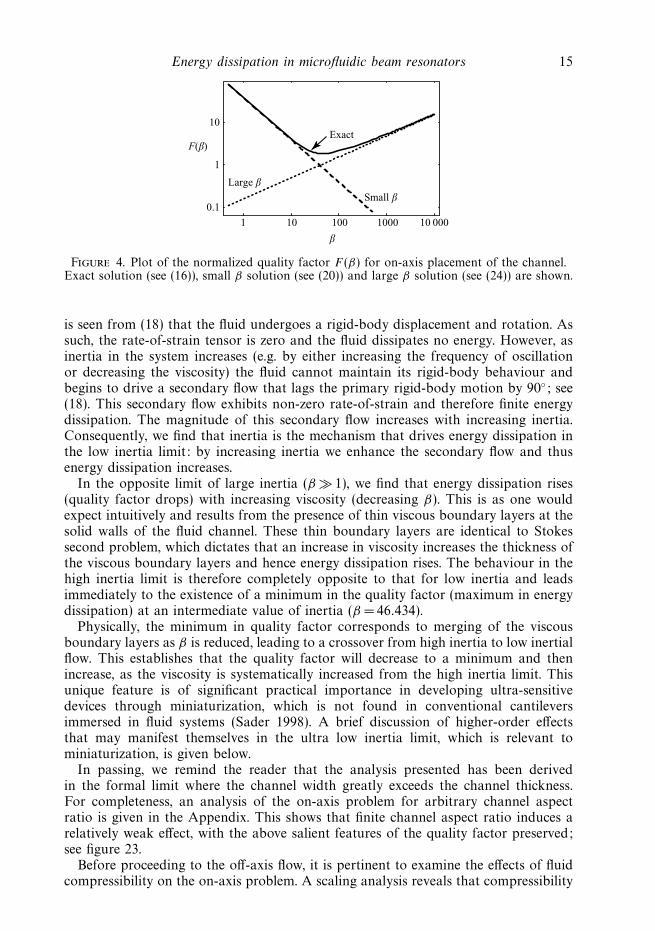
A comparison of the asymptotic solutions for F (β) in (20) and (24) and the exactsolution in (16) is given in figure 4. Note that the exact solution follows the correctasymptotic behaviour in the limits of small and large Reynolds number β , as required.Interestingly, the quality factor exhibits a non-monotonic dependence on β: (i) forβ 1, the quality factor increases with decreasing β , whereas (ii) for β 1, it increaseswith increasing β . The result is that the quality factor possesses a global minimum ofF =1.8175 at β = 46.434.

The physical origin of this unusual behaviour can be explained as follows. Webegin by examining the limit of small inertia (β 1), which exhibits the apparentlycounter-intuitive result that an enhancement in viscosity (reduction in β) reducesenergy dissipation (increases the quality factor). In the formal limit of zero inertia, it


1 10 100 1000 10 000

0.1

1

10

F(β)

Large β

Small β

Exact

β

Figure 4. Plot of the normalized quality factor F (β) for on-axis placement of the channel.Exact solution (see (16)), small β solution (see (20)) and large β solution (see (24)) are shown.

is seen from (18) that the fluid undergoes a rigid-body displacement and rotation. Assuch, the rate-of-strain tensor is zero and the fluid dissipates no energy. However, asinertia in the system increases (e.g. by either increasing the frequency of oscillationor decreasing the viscosity) the fluid cannot maintain its rigid-body behaviour andbegins to drive a secondary flow that lags the primary rigid-body motion by 90◦; see(18). This secondary flow exhibits non-zero rate-of-strain and therefore finite energydissipation. The magnitude of this secondary flow increases with increasing inertia.Consequently, we find that inertia is the mechanism that drives energy dissipation inthe low inertia limit: by increasing inertia we enhance the secondary flow and thusenergy dissipation increases.

In the opposite limit of large inertia (β 1), we find that energy dissipation rises(quality factor drops) with increasing viscosity (decreasing β). This is as one wouldexpect intuitively and results from the presence of thin viscous boundary layers at thesolid walls of the fluid channel. These thin boundary layers are identical to Stokessecond problem, which dictates that an increase in viscosity increases the thickness ofthe viscous boundary layers and hence energy dissipation rises. The behaviour in thehigh inertia limit is therefore completely opposite to that for low inertia and leadsimmediately to the existence of a minimum in the quality factor (maximum in energydissipation) at an intermediate value of inertia (β =46.434).

Physically, the minimum in quality factor corresponds to merging of the viscousboundary layers as β is reduced, leading to a crossover from high inertia to low inertialflow. This establishes that the quality factor will decrease to a minimum and thenincrease, as the viscosity is systematically increased from the high inertia limit. Thisunique feature is of significant practical importance in developing ultra-sensitivedevices through miniaturization, which is not found in conventional cantileversimmersed in fluid systems (Sader 1998). A brief discussion of higher-order effectsthat may manifest themselves in the ultra low inertia limit, which is relevant tominiaturization, is given below.

In passing, we remind the reader that the analysis presented has been derivedin the formal limit where the channel width greatly exceeds the channel thickness.For completeness, an analysis of the on-axis problem for arbitrary channel aspectratio is given in the Appendix. This shows that finite channel aspect ratio induces arelatively weak effect, with the above salient features of the quality factor preserved;see figure 23.

Before proceeding to the off-axis flow, it is pertinent to examine the effects of fluidcompressibility on the on-axis problem. A scaling analysis reveals that compressibility


will be important provided (ωL

c

)2 (hfluid

L

)2

∼ O(1).

Clearly, this condition is violated in the formal limit hfluid/L → 0 at fixed L, which isimplicitly assumed in the above analysis. Importantly, the condition is also violatedin cantilevers used in practice (Burg et al. 2007). This, therefore, establishes that fluidcompressibility is not important for the on-axis flow problem as has been assumed.

3.2. Off-axis flow problem

We now discuss the flow generated by off-axis placement of the channel. We considerthe off-axis problem only, which ignores the contribution from the on-axis flow field.

3.2.1. Incompressible flow

To begin, we examine the singular case of incompressible flow, which correspondsto α → 0. In the limits of small and large fluid inertia, the velocity field in (49)becomes

v = iωz0

dW

dx

∣∣∣∣x=L

x

⎧⎪⎨⎪⎩

1 + S(x)

[6

(z − z0

hfluid

)2

− 1

2

]: β → 0

1 : β → ∞+ O

(hfluid

L

).

(57)Equation (57) establishes that the velocity field possesses a parabolic distributionacross the channel thickness in the limit of small inertia (β 1), as may be expectedintuitively. In the opposite limit of high inertia (β 1), the flow field away from thechannel walls is plug flow, with fluid being pumped into and out of the channel in arigid-body fashion. This is also expected, because the channel walls will generate thinviscous boundary layers in this limit allowing the fluid away from the walls to movesynchronously with the end of the cantilever (x = L).

We now present numerical results for the flow field at finite inertia. Throughout,we consider the case where the length of the rigid lead channel equals the cantileverlength, as in the practical case (Burg et al. 2007, 2009), i.e. Lc = L. In figure 5, resultsare given for the velocity profile distribution in the channel corresponding to thelimits of small and large inertia. Note that the shear velocity gradient is greatest inthe rigid lead channel, and decreases as it approaches the end of the cantilever (x = L),as expected. The corresponding results for the pressure are given in figure 6, whereit is clear that the majority of the pressure drop (increase) occurs within the rigidlead channel for low inertia, whereas for high inertia the pressure drop is uniformlydistributed over the entire channel.

3.2.2. Compressible flow

Next, we include the effects of compressibility and study how this modifies theflow field. We again consider the practical case where the length of the rigid leadchannel equals the cantilever length, i.e. Lc = L. Note that practical cantilevers havea compressibility number α that lies in the range 0.01 <α < 1.

Figure 7 illustrates the effects of fluid compressibility on the velocity field formoderately small inertia β = 10. Note that compressibility can profoundly affect thevelocity field. A slight increase in compressibility, from the incompressible limit, leadsto a significant increase in fluid velocity entering the channel; see bottom-most tracesin figures 7(a)–7(e). Interestingly, as compressibility is increased further, a maximumvelocity is obtained (figure 7c) which then subsequently decreases.


–1

0

1

–1

0

1

x–

0–0.5 0.5

z–

(a)

–1

0

1

–1

0

1

0–0.5 0.5

z–

(b)

–1

0

1

–1

0

1

0–0.5 0.5

z–

(c)

–1

0

1

–1

0

1

0–0.5 0.5

z–

(d)

Figure 5. Velocity profile (magnitude) within the rigid channel/cantilever system. Variation influid velocity relative to wall velocity for x ∈ [−1, 1] and x =0.125. Notes: x = 0 correspondsto the clamped end of the cantilever. Velocity is scaled differently in rigid lead channel andcantilever, for presentation only. (a) β = 0.0001, (b) β = 10, (c) β = 100, (d ) β = 1000.

–1.0 –0.5 0 0.5 1.00

5

10

15

|P–| |P

–|

β = 0.0001

0

0.5

1.0

1.5

2.0

2.5

1

β

Increasing β

β = 10, 100, 1000

(a) (b)

x––1.0 –0.5 0 0.5 1.0

x–

Figure 6. Normalized pressure profile P (magnitude of (48)) within the rigid channel/cantilever system. Pressure scale used is Ps = μusL/h2

fluid and is appropriate for the low

inertia incompressible limit, i.e. β 1 and α 1; see (31). (a) β =0.0001, (b) β =10, β = 100,β = 1000.

To investigate the origin of this behaviour, we present results for the volumetricflow rate entering the rigid lead channel in figure 8 as a function of the acousticwavenumber γ , for a range of Reynolds numbers β . We remind the reader thatα = γ /β . For low inertia β = 1 (high viscous damping), the volumetric flux is seento decrease monotonically with increasing compressibility. However, as dampingis systematically reduced, by increasing β , this monotonicity in the volume fluxdisappears and is replaced with clear resonance behaviour. This explains the increasein fluid velocity observed in figure 7, which is due to the fundamental acousticresonance of the cantilever/rigid lead channel system, which occurs at αβ = γ = 0.28for β = 10.


–1

0

1

–1

0

1

x–

0–0.5 0.5z–

(a)

–1

0

1

–1

0

1

0–0.5 0.5z–

(b)

–1

0

1

–1

0

1

0–0.5 0.5z–

(c)

–1

0

1

–1

0

1

0–0.5 0.5z–

(d)

–1

0

1

–1

0

1

0–0.5 0.5z–

(e)

Figure 7. Velocity profile (magnitude) within the rigid channel/cantilever system showingeffects of compressibility. Variation in fluid velocity relative to wall velocity for x ∈ [−1, 1]and x = 0.125. Note: x = 0 corresponds to the clamped end of the cantilever. Moderately lowinertia: β =10. (a) α = 0, (b) α = 0.01, (c) α = 0.03, (d ) α = 0.05, (e) α = 0.1.

0.01 0.1 1 10 100

1

(a) (b)

(c) (d)

10–2

10–4

10–6

10–8

10–10

β = 1

γ γ

Norm

aliz

ed v

olu

met

ric

flux

0.01 0.1 1 10 100

0.01 0.1 1 10 100 0.01 0.1 1 10 100

1

10–1

10–2

10–3

10–4

β = 10

0.2

0.5

1.0

2.0

5.0 β = 100

Norm

aliz

ed v

olu

met

ric

flux

1

2

3

5

10

20 β = 1000

Figure 8. Normalized magnitude of volumetric flux into rigid lead channel as a function ofthe normalized wavenumber γ . (a) β = 1, (b) β =10, (c) β = 100, (d ) β = 1000. Volumetric fluxscale is qs = ushfluidbfluid .

Note that this resonance behaviour is strongly dependent on β , and for low β

the system can become overdamped, leading to no observed resonance. Indeed, it isfound that for fixed β , the number of resonances is finite, with the system becomingincreasingly damped with increasing mode number, e.g. see figure 8(c), where only sixresonance peaks are present for all γ .


–1

0

1

–1

0

1

x–

0–0.5 0.5z–

(a)

–1

0

1

–1

0

1

0–0.5 0.5z–

(b)

–1

0

1

–1

0

1

0–0.5 0.5z–

(c)

–1

0

1

–1

0

1

0–0.5 0.5z–

(d)

–1

0

1

–1

0

1

0–0.5 0.5z–

(e)

Figure 9. Velocity profile within the rigid channel/cantilever system showing effects ofcompressibility. Variation in fluid velocity relative to wall velocity for x ∈ [−1, 1] andx = 0.125. Note: x = 0 corresponds to the clamped end of the cantilever. Low inertia:β = 0.0001. (a) α = 0, (b) α =0.01, (c) α =0.03, (d ) α =0.05, (e) α = 0.1.

–1.0 –0.5 0 0.5 1.0–15

–10

–5

0

Increasing αIncreasing α Increasing α

Re{

P– }

Im{P– }

–8

–6

–4

–2

0

0

5

10

15(a) (b) (c)

x––1.0 –0.5 0 0.5 1.0

x––1.0 –0.5 0 0.5 1.0

x–

|P– |

Figure 10. Normalized pressure profile P within the rigid channel/cantilever system showingeffects of compressibility. Pressure scale used is Ps = μusL/h2

fluid and is appropriate for

the low inertia limit, i.e. β 1 and α 1; see (31). Low inertia: β = 0.0001. α = 0.0001,0.01, 0.03, 0.05, 0.1. (a) Real (in-phase with wall velocity) component; (b) imaginary(out-of-phase with wall velocity) component; (c) absolute value.

To further illustrate the above-described damping effect, figure 9 presents resultsfor the velocity field at very low inertia β =0.0001, for which no resonance behaviouris observed; in contrast to the results presented in figure 7 (for moderately smallinertia), the magnitude of velocity at the channel entrance (x = − 1) decreasesmonotonically with α. The corresponding pressure profile throughout the channelis given in figure 10. Note that as compressibility is increased, i.e. α increases, thedissipative (real) component of the scaled pressure decreases in magnitude. Forα � 0.03, the pressure gradient reverses sign, which drives the flow in the oppositedirection. This feature is manifested in figure 9. We thus find that the fluid velocityrelative to the wall moves in the opposite direction near the free end of the cantileverto that in the rigid channel. In contrast, the inertial (imaginary) component of thepressure increases with increasing α due to the increased elasticity of the fluid system.The overall effect of compressibility is to reduce the magnitude of the pressure dropleading to lower volumetric flux into the cantilever.

Although the above variations in parameter space serve to illustrate the dominanteffects of compressibility, through the compressibility number α, they are difficult torealize experimentally since this would require fluids with different speeds of sound.


–1

0

1

–1

0

1

x–

0–0.5 0.5

(a)

–1

0

1

–1

0

1

0–0.5 0.5

(b)

–1

0

1

–1

0

1

0–0.5 0.5

(c)

–1

0

1

–1

0

1

x–

0–0.5 –0.50.5

z–

(d)

–1

0

1

–1

0

1

0 0.5

z–

(e)

–1

0

1

–1

0

1

0–0.5 0.5

z–

(f)

Figure 11. Velocity profile within the rigid channel/cantilever system as viscosity is variedfor fixed fluid density. Variation in fluid velocity relative to wall velocity for x ∈ [−1, 1] andx = 0.125. Note: x = 0 corresponds to the clamped end of the cantilever. γ = 0.03. Increasingβ from left to right. (a) β = 0.01, (b) β = 0.03, (c) β = 0.1, (d ) β = 0.3, (e) β = 1, (f ) β = 10.

An alternative approach to enhance the effects of compressibility is to increase theviscosity while holding the speed of sound and density of the fluid constant. This iseasily achieved in practice, because the speed of sound of most liquids is comparable.In this case, γ is fixed and β (and hence α = γ /β) changes as the viscosity varies.We consider the typical case where γ = 0.03 (which is identical to the 3 μm channelthickness cantilever investigated in § 3.4). Figure 11 shows the velocity profile in theentire channel system under these conditions.

Note that increasing viscosity corresponds to decreasing β . The effects of fluidcompressibility are clear in figure 11 and demonstrate that they can profoundlyinfluence the flow. The results for β =1 and β =10 are essentially the incompressiblesolution for low β exhibiting parabolic velocity profiles. However, as the viscosityincreases (β decreases), the pressure also increases and ultimately becomes largeenough to significantly compress the fluid. This reduces the volumetric flow rate intothe channel system since the fluid is able to intrinsically accommodate the volumevariations in the cantilever as it oscillates. We also note that flow reversal becomes


β = 0.01

10

1

0.3

0.1

0.03 10

1

0.3

0.1

0.03

β = 0.01 101

0.3

0.1

0.03

β = 0.01

–1.0 –0.5 0 0.5 1.0

–0.2

–0.4

0

0.2

0.4R

e{P– }

Im{P– }

–1.5

–1.0

–0.5

0

0

0.5

1.0

1.5(a) (b) (c)

x––1.0 –0.5 0 0.5 1.0

x––1.0 –0.5 0 0.5 1.0

x–

|P– |

Figure 12. Normalized pressure profile P within the rigid channel/cantilever system showingeffects of compressibility. Pressure scale used is Ps = μusL/h2

fluid/α and is appropriate for the

low inertia compressible limit, i.e. β 1 and α = γ /β 1. Resonator parameters: γ = 0.03.β = 0.01, 0.03, 0.1, 0.3, 1, 10. Pressure variation increases with decreasing β . (a) Real (in-phasewith wall velocity) component; (b) imaginary (out-of-phase with wall velocity) component; (c)absolute value.

0.001 0.01 0.1 1 10 100

0.1

0.3

1

3

10

0.03

Ediss

β

γ = 0.01

0.03

0.1

0.3

1

Figure 13. Normalized rate of total energy dissipation per unit cycle for variousγ = 0.01, 0.03, 0.1, 0.3, 1. Observed maxima shift to right in β space with increasing γ in

accord with resonance condition α = γ /β ∼ O(1). Energy scale is Es = 4πρ0Lbfluidhfluid |us |2.

present in the flow and the shear velocity gradients decrease in magnitude as a resultof compressibility.

The velocity variations as a function of viscosity in figure 11 can be understoodthrough an examination of the pressure distribution in the fluid channel/cantileversystem. Figure 12 shows the (scaled) pressure variation in the whole channel systemunder the conditions specified in figure 11; the pressure scaling differs from thatused in figure 10. Note the correlation between the real component of the pressure(in-phase with the wall velocity) and the velocity behaviour in the fluid. As theeffects of compressibility increase (β decreases), the real component of the pressureand pressure gradient change sign, and this drives the flow in alternate directions.Interestingly, the magnitude of this component is approximately independent of β ,for β � 1. In contrast, the magnitude of the imaginary component (out-of-phase withthe wall velocity) and the total magnitude of the pressure increase with decreasing β .

3.2.3. Energy dissipation

In figure 13 we present results for the (scaled) rate of energy dissipation in thechannel due to off-axis flow for γ ∈ [0.01, 1]. Note that α = γ /β , and hence increasingβ reduces the effects of compressibility; see (32). In the limit of large inertia (β 1),we find that the energy dissipated decreases with increasing β , as is expected for


incompressible flow; increasing β can be easily achieved in practice by reducing theviscosity while holding the density constant. However, in the asymptotic limit β 1,the energy dissipated decreases with decreasing β; see § 3.5 for a discussion of higher-order mechanisms at small β that are not included in the present model. This latterphenomenon is due to the increasing effects of compressibility that limit the volumeflux into the channel and hence reduce the rate-of-strain as illustrated in figure 11.In the intermediate regime α = γ /β ∼ O(1), we find that energy dissipation featurestwo maxima, with a local minimum between these peaks. The mechanism for thisbehaviour arises from competing dissipative effects in the rigid lead channel and thecantilever proper, as we now discuss.

Rigid lead channel (x < 0). To begin, we focus on the rigid lead channel and considerthe asymptotic limit of incompressible flow α 1, which corresponds to β 1 at fixedγ . As viscosity increases in the high inertia limit, the Reynolds number β decreaseswhereas the normalized acoustic number γ remains fixed. In this incompressiblelimit, energy dissipation rises with increasing viscosity. However, the pressure alsorises simultaneously and ultimately reaches a level where it can significantly compressthe fluid. This reduces the shear velocity gradients, which in turn reduces energydissipation. Energy dissipation ultimately approaches zero with increasing viscosity.These competing effects lead to the overall feature of an enhancement of energydissipation at high inertia, and a reduction at low inertia as the viscosity increases(β decreases). This in turn explains the existence of a maximum in energy dissipationat intermediate β .

Cantilever proper (x > 0). We now examine energy dissipation in the cantileverproper. Unlike the rigid lead channel, the peak in energy dissipation does not occurat the transition point from incompressible to compressible flow, but is due to a peakin flow reversal that results from compressibility effects. To understand this, we notethat as viscosity increases, the pressure rises high enough to significantly compressthe flow and this leads to reversal in the pressure gradient. This in turn results inflow reversal in this region (see figures 11 and 12) and thus a reversal in the sign ofthe shear velocity gradients. Importantly, in the limit of infinite compressibility, theshear velocity gradients are zero. As such, there must exist an intermediate value ofviscosity that leads to a maximum in the reversed flow velocity and hence a maximumin energy dissipation. This salient feature explains the existence of maximum energydissipation at intermediate values of β for this region (x > 0). In general, this criticalvalue of β differs from that for the rigid lead channel discussed above. This shift inthe position of the maximum in the cantilever proper explains the double humpedfeature in figure 13, which is obtained by superimposing the energy dissipation in thecantilever proper (x > 0) and rigid lead channel (x < 0). The distribution of energydissipation throughout the cantilever/rigid channel system shown in figure 14 revealsthat the rightmost maximum in β space is due to the rigid lead channel, whereas theleftmost maximum is due to the cantilever proper. Variation in the shape of the totalenergy dissipation curves in figure 13 for increasing γ is due to the increasing effectsof fluid inertia at large values of β .

The competing compressibility effects in the rigid lead channel and cantileverproper, which lead to maxima at different values of β , thus give rise to a localminimum in the energy dissipated at intermediate values of β . Importantly, theabove discussion establishes that the rightmost maximum in β space results fromenhancement in the magnitude of the pressure, whereas the leftmost maximum iscaused by the pressure gradient (not the magnitude of the pressure). This featureallows for tuning of the positions of these two maxima in β space, by appropriateadjustment of the dimensions of the cantilever/lead channel system. As such, the β


–0.5

0.5

–1.0

020406080

100

0

–0.5

0

0.5

1.0

Wdiss

x–

z––0.5

0.5

–1.0

020406080

100

0

–0.5

0

0.5

1.0

Wdiss

x–

z––0.5

0.5

–1.0

020406080

100

0

–0.5

0

0.5

1.0

Wdiss

x–

z–

–0.5

0.5

–1.0

020406080

100

0

–0.5

0

0.5

1.0

Wdiss

x–

z–

–0.5

0.5

–1.0

020406080

100

0

–0.5

0

0.5

1.0

Wdiss

x–

z––0.5

0.5

–1.0

020

6040

80100

0

–0.5

0

0.5

1.0

Wdiss

x–

z–

(c)(b)(a)

(f)(e)(d)

Figure 14. Normalized rate of energy dissipation distribution (per unit volume) for γ = 0.01and increasing β = 0.001, 0.003, 0.01, 0.03, 0.1, 1 (a–f ). Energy (per unit volume) scale is

Ws = 4πρ0 |us |2.

distance between the observed local maxima in energy dissipation will depend on theratio of the cantilever length L to that of the rigid lead channel Lc. This feature isillustrated in figure 15. Note that the position of the leftmost maximum is independentof Lc/L (at fixed cantilever length L), as expected, because this arises from flow inthe cantilever proper (x > 0). The rightmost maximum, however, depends strongly onLc/L, because by changing the length Lc of the rigid lead channel, its contributionto the total energy dissipation is enhanced or reduced. By increasing the length ofthe rigid channel Lc, the position of the rightmost maximum occurs at higher valuesof β , because this enhances the pressure in that region leading to an earlier onset ofcompressibility effects. Thus, increasing the rigid channel length amplifies the effectof compressibility as expected. The enhanced topmost curve in figure 15 results fromstrong overlap in the flow within the cantilever proper and rigid channel, due to ashort rigid lead channel.

Maximum pressure. We continue our discussion of the off-axis flow problem byexamining the maximum pressure generated in the fluid channel. The pressure invarious practical flow regimes scales in the following manner with respect to theexplicit cantilever and fluid properties:

P ∼

⎧⎪⎪⎪⎪⎪⎨⎪⎪⎪⎪⎪⎩

μω

(z0

hfluid

)(a

hfluid

): β 1, α 1 (low inertia, incompressible),

ρ0ω2z0a : β 1, γ 1 (high inertia, incompressible),

ρ0c2(z0

L

) ( a

L

): β 1, α 1 (low inertia, compressible),

(58)


0.001 0.01 0.1 1

3

10

2

5

20

β

Ediss

Lc / L = 0.5

0.75

1

1.5

2

Figure 15. Normalized rate of total energy dissipation for γ = 0.01 and various ratiosLc/L = 0.5, 0.75, 1, 1.5, 2. Lc/L increases from top to bottom curves. Energy scale is thesame as in figure 13.

0.01 0.1 1 10 100

0.003

0.01

0.03

0.1

0.3

1.0

β

Increasing γ

|P–

max|

Figure 16. Magnitude of normalized maximum pressure∣∣Pmax

∣∣ within the rigid chan-nel/cantilever system for various normalized acoustic numbers γ = 0.001, 0.003, 0.01, 0.03, 0.1.Pressure scale is Ps = ρ0c

2us/(ωL) and is appropriate for the low inertia compressible limit, i.e.β 1 and α 1; see (58). Length of the rigid lead channel equals the cantilever length, i.e.Lc = L.

where a is the amplitude of oscillation. Note that numerical factors are ignoredin (58). From (58), we see that increasing the oscillation amplitude, a, and off-axisplacement, z0, of the fluid channel always enhances the maximum pressure, as required.Figure 16 gives results for the magnitude of the maximum normalized pressure inthe fluid channel as a function of fluid inertia and compressibility. The pressure scalein the low inertia compressible limit (β 1, α 1) is used throughout, because thisdoes not change as the cantilever is (i) uniformly reduced in size, nor (ii) as the fluidviscosity is varied. Both situations are considered below.

From figure 16, we observe that as the fluid viscosity is increased (β decreases),the maximum pressure also increases as expected. This is particularly pronouncedin the low inertia regime (β <O(1)) where the viscous boundary layers generated atthe surfaces strongly overlap. In the limit of very low inertia (β 1), the pressure ishigh enough to induce significant dilation of the fluid, and this relaxes the monotonicincrease in pressure as viscosity is increased note that the normalized maximumpressures are of order unity in this limit, as required by the pressure scale chosen.

Next, we examine the effects of miniaturization on the maximum pressure. From (33)we find that as the cantilever geometry is uniformly reduced in size, the characteristic


dimensionless parameters for the flow vary according to the following scaling relations:

β ∼ hcant

(hfluid

L

)2

, γ ∼(

hcant

L

)2

, α ∼ 1

hfluid

(hcant

hfluid

). (59)

From these relations it is clear that the effects of compressibility are enhanced as thecantilever is miniaturized (α increases), while the effects of fluid inertia are reduced(β decreases). In contrast, the normalized wavenumber γ remains constantthroughout, indicating that the acoustic properties of the flow are unperturbed byminiaturization. From figure 16, it follows that miniaturization, which results in areduction in β at constant γ , will in turn enhance the maximum pressure in thedevice.

Cavitation. Using the results presented in figure 16 for the off-axis flow maximumpressure, we now assess the possibility of inducing cavitation in the fluid channel.This is expected to occur when the maximum (negative) pressure, generated by thecantilever oscillation, decreases the ambient pressure below the vapour pressure ofthe liquid contained in the channel; see Batchelor (1974) for further discussion. Sincethe vapour pressure of water and glycerol at room temperature is well below 1 atm(∼100 kPa), this requires the maximum pressure to be comparable to 1 atm.

We note that pressure due to the on-axis flow scales as ρ0ω2hfluida, and is always

given by the inviscid flow result in (9). Significant pressures can also be generated bythe on-axis flow, but are normally smaller than those that can be generated by theoff-axis flow. The effects of on-axis flow are thus not considered here.

For the purpose of illustration, we consider one of the cantilevers studied by Burget al. (2009); see cantilever B in § 3.4, where its dimensions are listed. We assume atypical oscillation amplitude of a = 100 nm throughout. For water, the dimensionlessparameters are β =12 and γ = 0.035, and a maximum pressure of 2.1(z0/hfluid ) kPais obtained, where z0 is the off-axis placement of the fluid channel as specified above.Note that the maximum off-axis placement in any device is z0 = (hcant − hfluid )/2;for this cantilever device (z0/hfluid )max = 2/3. Therefore, regardless of the choice ofoff-axis placement, the maximum pressure induced in water is well below the pressurerequired to achieve cavitation. Using pure glycerol, we find β = 0.010 and γ = 0.023,and a maximum pressure of 47(z0/hfluid ) kPa. Therefore, even if the fluid channel isplaced as far as possible from the neutral axis of the beam, i.e. z0/hfluid is maximized,pressures in excess of 1 atm in glycerol are not predicted to be possible. Therefore,current devices are thus not prone to these effects.

From (58), it is clear that to increase the maximum pressure, the cantilever mustbe made shorter (thus increasing the resonant frequency), and the off-axis channelposition z0 and oscillation amplitude a increased.

If the length L of cantilever B is reduced to 100 μm, while keeping all otherdimensions identical, the picture changes dramatically. Using water, the dimensionlessparameters are β = 54 and γ = 0.16, and the maximum pressure becomes 47(z0/hfluid )kPa. Since the maximum off-axis placement in this device is (z0/hfluid )max = 2/3, themaximum possible pressure is 31 kPa, which is approximately a third that requiredto induce cavitation. However, using pure glycerol, we obtain β = 0.045 and γ = 0.10,and a maximum pressure of 210(z0/hfluid ) kPa; cavitation is therefore possible in thislatter case.

Further reduction in length to 50 μm yields 1900(z0/hfluid ) kPa and 840(z0/hfluid )kPa in water and pure glycerol, respectively. As such, even a small off-axis placement


of the fluid channel is predicted to allow for cavitation in both water and pureglycerol.

Finally, we note that the model implicitly assumes that fluid density variations dueto compressibility are small, allowing for linearization of the governing equationsand equation of state. Pressures in the vicinity of 1 atm induce density variationsof less than 0.01 %. Thus, the underlying model assumptions remain intact whenexploring the onset of cavitation. Once cavitation is achieved, however, the continuumapproximation breaks down and applicability of the model must be drawn intoquestion.

3.3. Complete flow

We now combine the flow fields for the on-axis and off-axis problems to obtain thecomplete flow for the cantilever/rigid lead channel system. To begin, we examine thelimiting case of incompressible flow and study the energy dissipation in the system.

3.3.1. Incompressible flow

We again focus on the normalized quality factor F (β). In the limits of small andlarge inertia, the asymptotic behaviour of this function for the fundamental mode ofvibration can be explicitly derived from the exact solution

F (β) =

⎧⎪⎪⎪⎪⎨⎪⎪⎪⎪⎩

38.73β

β2 + 564.6Z20

(1 +

β2

8400

) : β → 0,

√β

6.573 + 1.718Z20

: β → ∞.

(60)

Equation (60) clearly demonstrates that off-axis placement of the channel can exert astrong influence on the quality factor. The overall effect as the viscosity is varied willnow be described. We restrict ourselves to the case where the off-axis position of thechannel Z0 is non-zero and significantly less than one channel thickness, i.e. Z0 1,which is the practical case commonly encountered. Note that decreasing the viscosity(at constant density) will increase β .

Starting in the low inertial limit, we observe from (60) that the quality factorwill increase with increasing β , i.e. decreasing viscosity. In this regime, oscillatoryinflow/outflow within the channel, due to off-axis placement, dominates the inertialmechanism for dissipation previously described for on-axis channels. Importantly, thisadditional flow has a non-zero effect in the limit of zero fluid inertia, which gives riseto a strong deviation from the on-axis result in the limit as β → 0. This behaviour ispresent for β <βmax , where

βmax = 23.76Z0 + O(Z2

0

). (61)

Note that this asymptotic formula is a good approximation for Z0 < 0.5, exhibiting amaximum error of 14 %.

At the critical point (β = βmax), the quality factor attains a local maximum value.Importantly, for off-axis positions significantly less than one channel thickness(Z0 1), this critical value for β is smaller than that required for the minimumquality factor predicted by (31), i.e. βmin = 46.434. Consequently, increasing β furtherwill decrease the quality factor, with the inertial mechanism previously described foron-axis flow dominating the inflow/outflow in the channel, until a minimum qualityfactor is reached at βmin =46.434. Further increase in β will then enhance the qualityfactor as before. These salient features of the quality factor are illustrated in figure 17.


0.1 1 10 102 103 104

0.1

1

10

Large β

Small β

Exact

Z–

0 = 0.1F(β)

β

Figure 17. Plot of F (β) function for quality factor. Exact solution (see (56a)), small β solution(see (60)) and large β solution (see (60)) are shown. Results for off-axis placement: Z0 = 0.1.

The results in figure 17 for the case of off-axis placement are to be comparedwith those in figure 4 for on-axis placement. Note that the dominant features of thequality factor profile are accurately predicted by the asymptotic results in figure 17.We also observe that off-axis placement dominates the behaviour only for low inertia,i.e. small β .

Importantly, the above-described turnover in the quality factor (see figure 17) atintermediate values of β disappears for

Z0 ≡ z0

hfluid

> 0.64515, (62)

at which point the quality factor increases monotonically with increasing β .

3.3.2. Compressible flow

The effects of compressibility on energy dissipation are now included. Importantly,compressibility will only affect the velocity field for the off-axis flow problem, asdiscussed above. However, since the total flow is given by superposition of the off-axis and on-axis problems, compressibility can affect the entire quality factor. Infigure 18, results are presented for a typical normalized wavenumber of γ = 0.03,and for a range of different off-axis positions Z0 ∈ [0, 0.1]. Again, we consider thepractical case where Lc = L.

Note that the quality factor in figure 18 is unaffected by off-axis channel placementfor β > βmin = 46.434, and is therefore independent of fluid compressibility. Thisindicates that inertial effects present in the on-axis flow problem dominate anyoff-axis phenomena. The behaviour for β < βmin = 46.434, however, is dramaticallydifferent and is strongly influenced by fluid compressibility; cf. figures 17 and 18for Z0 = 0.1. The incompressible solution displays a clear maximum in quality factorat β ≈ 1, whereas the compressible solution shows two local maxima at β ≈ 10 andβ ≈ 0.1, and ultimately a uniform increase as β decreases. This demonstrates thateven for small off-axis channel placement, fluid compressibility can have a profoundeffect.

Once compressibility begins to affect energy dissipation with decreasing β , thequality factor remains approximately constant over decades in β . We also observethat the quality factor exhibits small oscillations in magnitude as β varies; this is inline with the energy dissipation results for the off-axis flow problem; cf. figures 13and 18.


0.01 1 102 104

1

3

10

30

100

300Z–

0 = 0

0.01

0.02

0.1

β

γ = 0.03

F(β)

Figure 18. Plot of F (β) function for quality factor for compressible flow (γ = 0.03). Exactsolution (see (56a)), small β solution (see (60)) and large β solution (see (60)) are shown.Results for various off-axis placement: Z0 ∈ [0, 0.1] in increments of 0.01. The top curvecorresponds to Z0 = 0.

0.01

0.1

1

101

102

103

104

γ = 0.03

0.01

0.1

1

0.02

0.05

0.2

0.5

F(β)

0.01 1 102 104

β

Z–

0 = 0

Figure 19. Same as figure 18 for Z0 ∈ [0, 1] in increments of 0.1. The top curvecorresponds to Z0 = 0.

In figure 19, we examine these effects for larger Z0 corresponding to off-axischannel placements up to one channel thickness. From these results it is clear thatthe quality factor always ultimately increases at lower β , regardless of the value ofZ0. This behaviour contrasts directly with that for incompressible flow, for which thequality factor decreases monotonically with decreasing β for small β . We also see aslight reduction in the quality factor for β >βmin =46.434, which is in line with theincompressible result; see (60).

As β decreases below βmin, we can observe two distinct local maxima in figures 18and 19. The position of the maximum closest to βmin = 46.434 corresponds to theonset of the effects of off-axis channel flow, which enhances dissipation due to thepumping of fluid into and out of the channel. The second maximum furthest fromβmin occurs at a single value of β , regardless of the off-axis channel position Z0

and coincides with the energy dissipation minimum discussed in figure 13; note thatenergy dissipation is inversely proportional to the quality factor. We remind the readerthat this phenomenon originates from competing compressibility effects in the off-axis


0.01

(a) (b)

0.1

1

101

102

0.1

1

101

102

104γ = 0.010.01

0.02

0.1

1

0.05

0.2

0.5

γ = 0.10.01

0.02

0.05

0.1

1

0.2

0.5

F(β)

Z–

0 = 0 Z–

0 = 0

0.01 1 102 104

β

0.01 1 102 104

β

Figure 20. Same as figure 19 for γ = 0.01, 0.1.

0.001 0.01 0.1 1

0.3

0.4

0.5

0.6

αmax

γ

Increasing Z–

0

Z–

0 = 0.1, 0.5, 1,∞

Figure 21. Plot showing variation in αmax as a function of γ for Z0 = 0.1, 0.5, 1, ∞. Valuefor αmax decreases with increasing Z0.

channel system and occurs at α = γ /β ∼ 0.3. Note that we require α ∼ O(1) for theeffects of fluid compressibility to be significant; see (32).

In figure 20, we examine the effects of varying compressibility at fixed off-axischannel position Z0. Note that compressibility significantly modifies the behaviourfor β < βmin = 46.434 and reduces dissipation due to off-axis channel placement, i.e. thequality factor increases with increasing γ . Furthermore, the maxima in F (β) previouslyobserved for incompressible flow are displaced in β space. In particular, the leftmostmaximum arising from competing compressibility effects in the off-axis problem nowappears at different values of β . Significantly, the value of α at which this maximumoccurs is approximately constant regardless of the value of Z0 and γ for γ < 0.1, asillustrated in figure 21. In this regime, the maximum occurs at

αmax =γ

β=

ωμ

ρc2

(L

hfluid

)2

= 0.287, γ → 0. (63)

The observed increase in αmax for higher values of γ is due to inertial effects in thefluid becoming increasingly important; note that β increases with increasing γ sinceβ = γ /α. Importantly, the physical origin of this maximum is independent of theon-axis problem, but the competing effects of the on-axis and off-axis problems canaffect the position of this maximum. This explains the observed deviation in αres withdecreasing Z0. In the formal limit Z0 → ∞, αres plateaus to a constant value for fixedγ ; see figure 21.


10

(a) (b)

7

5

3

2

Incompressible

Incompressible

Compressible

Compressible

Measurements

Measurements

hfluid = 8.6 μm

hfluid = 8 μm hfluid = 3 μm

hfluid = 7.4 μmhfluid = 3.3 μm

hfluid = 2.7 μm

0.1 1 10 100

F(β)

2

1

0.7

0.5

0.3

β

0.01 0.1 1 10

β

Figure 22. Comparison of theoretical models (lines) with measurements (circles) for cantileverA and B defined below. A glycerol/water mixture was used. Compressible model (solid line);upper trace: speed of sound c = 1500m s−1 (water), lower trace c = 1850 m s−1 (glycerol).Incompressible model (dashed line). Systematic uncertainty in fluid channel thickness usedto evaluate F (β) from measurements of Q is indicated; see (55). This uncertainty allows thecentral large dots to be collectively shifted within the prescribed bounds, along the slantedlines, as shown. Q measured to < 1 % uncertainty (Burg et al. 2009). (a) Cantilever A with 8μm channel (Z0 = 0.06); (b) cantilever B with 3 μm channel (Z0 = 0.14).

3.4. Experiments and comparison

We now compare the predictions of the above theory with measurements taken on twodifferent cantilevers using a glycerol/water mixture; this enables the inertia parameterβ to be varied over 3 orders of magnitude. The two cantilevers have different fluidchannel and cantilever thickness, but are identical otherwise. The oscillation amplitudewas systematically varied to ensure that the linear limit was observed. In all cases, themeasured quality factors and resonant frequencies were found to be independent ofthe oscillation amplitude as required; maximum oscillation amplitude used was ∼50nm. The measured quality factors in the presence and absence of liquid are given infigure 2 of Burg et al. (2009), and all other experimental details are included in thatreference.

Properties of the two cantilevers used are:A. Channel: hfluid = 8±0.6 μm, bfluid = 16±0.25 μm, L =204±0.5 μm, Lc = 207.5±

0.25 μm; Cantilever: hcant = 12 ± 1.5 μm, bcant = 33 ± 0.25 μm, length: 210 ± 0.5 μm,resonant frequency (cantilever filled with air): fres =426.8 kHz.

B. Channel: hfluid = 3 ± 0.3 μm, bfluid = 16 ± 0.25 μm, L = 204 ± 0.5 μm, Lc =207.5 ±0.25 μm; Cantilever: hcant = 7 ± 1.5 μm, bcant = 33 ± 0.25 μm, length: 210 ± 0.5 μm,resonant frequency (cantilever filled with air): fres =212.5 kHz.

Since off-axis placement Z0 of the fluid channel is unknown, it is used as a fittingparameter in the following comparison. Critically, the theoretical solution dependsstrongly on Z0, as illustrated in figures 18–20. This enhances the precision in fittingZ0, which can then be compared with expected values due to fabrication tolerances,as we shall discuss below.

The precision of measured values for F (β) shown in figure 22 is primarily limited bythat of the channel thickness hfluid (which is known to within ∼10 %). This is becausethe relation between the quality factor Q and F (β) depends on the cube of hfluid ;see (55). Systematic uncertainty in hfluid will therefore collectively shift the measuredvalues of F (β), as illustrated in figure 22; small open circles indicate the bounds ofthis shift, whereas the large circles indicate the expected values. The statistical errorin measurements of Q is less than 1 % (see Burg et al. 2009) and is indiscernible in


2

5

10

20

50

Increasing Achannel

Achannel = 1,2,5,∞

F(β)

1 101 102 103 104

β

Figure 23. Plot of F (β) function for quality factor as a function of the channel aspect ratioAchannel using the exact solution (A 2).

figure 22. As such, the observed variations in the measured F (β) as a function of β ,for a fixed hfluid , completely dominate the measurement error.

In figure 22(a), we present a comparison of the theoretical model with measurementsfor cantilever A, which possesses a fluid channel of square cross-section. We remindthe reader that the model is derived using an Euler–Bernoulli/lubrication formulation,and as such, is formally valid for cases where the cantilever length L greatly exceedsthe cantilever width bcant , and where the channel width bfluid greatly exceeds itsthickness hfluid . Cantilever A possesses the properties L/bcant ≈ 6 and bfluid/hfluid ≈ 2,which is somewhat outside the expected regime of validity of the model. Nonetheless,we observe from figure 22(a) that the (compressible) model predicts the salient featuresof the response, when a (scaled) off-axis channel position of Z0 = 0.06 is chosen. Thiscorresponds to Z0 = 0.5 μm, which is in line with the expected uncertainty in themicrofabrication process; note that Z0 cannot be measured directly in these devices.For completeness, variations in the fluid compressibility between the expected boundsfor glycerol/water are also shown in figure 22 (shaded regions). This results ina relatively minor variation in comparison to the incompressible theory, which isunable to describe the measurements in the low β regime, regardless of the choiceof Z0.

Interestingly, we find that at high β , the measured quality factor exceeds the modelprediction, indicating that dissipation in the real system is less than that predicted.Use of the arbitrary channel aspect ratio theory (see the Appendix) in this regimedoes not reconcile theory and measurements; cf. figures 22(a) and 23. Importantly, thearbitrary channel aspect ratio theory in the Appendix still requires that the cantileverlength greatly exceed its width, and as such, the comparison between theory andmeasurements indicates that finite L/bcant and L/hcant effects may be behind theobserved discrepancy between theory and measurements.

A possible explanation for this observed reduction in dissipation (higher Q) incomparison to the theoretical model is now outlined. A cantilever of finite lengthis expected to provide extra constraints on the on-axis flow, particularly at the freeend of the cantilever where the flow must move in tandem with the beam. Thiswill reduce the strain rate in that region (of maximum amplitude) and decrease theoverall energy dissipation; this is observed in both the low and high β incompressibleon-axis regimes (3 < β < 300). For lower β , the off-axis (pumping) flow dominates andthe model yields results in reasonable agreement with measurements. We emphasize,however, that the precise mechanism giving rise to the measured discrepancy can only


be rigorously established by calculating the next order correction for finite L/bcant

and L/hcant ; see § 3.5.Complementary results for cantilever B are given in figure 22(b). In comparison

to cantilever A, this cantilever possesses a significantly thinner fluid channel withbfluid/hfluid ≈ 5. We note that the agreement between theory and measurements isgreatly improved, with the model accurately predicting the features of the measuredresponse. In this case, an off-axis channel position of Z0 = 0.14 (Z0 = 0.4 μm) isrequired to yield good agreement between measurements and theory; this absoluteoffset is similar to that for cantilever A and is again in line with expecteduncertainty in channel placement. This improvement in agreement is consistent withthe assumption inherent in the model that the fluid channel width greatly exceeds itsthickness. Again, we find that the incompressible theory is incapable of predicting themeasurements with the leftmost maximum in figure 22(b) absent (see dashed line).Fluid compressibility is therefore found to be of paramount importance in describingthe dynamics of these devices, and the above comparisons serve to demonstrate thevalidity of the new model.

It is important to note that the quality factor due to dissipation in the fluid can becomparable in magnitude to the intrinsic quality factor of the cantilever structure, asobserved by Burg et al. (2007). This feature can result in identical quality factors whenair or water is used, as we now discuss. Injecting water into the fluid channel increasesthe mass of the cantilever, which lowers the resonant frequency. This increases theintrinsic quality factor (since it is a scaled quantity) provided the intrinsic dampingcoefficient is frequency independent, which is assumed in the above experimentalcomparison. As a result, the intrinsic quality factor of the device with water in thechannel is higher than that with air, i.e. Qintrinsic

WATER >QintrinsicAIR . Importantly, the fluid

quality factor for air is orders of magnitude higher than the intrinsic quality factorQintrinsic

AIR , whereas for water the intrinsic and fluid quality factors are of comparablemagnitude. The net effect is that the total quality factor in air is well described bythe intrinsic value Qintrinsic

AIR , whereas in water the total quality factor is lower thanQintrinsic

WATER . These competing effects can conspire to give identical quality factors in airand water, as observed by Burg et al. (2007).

3.5. Further theoretical considerations

We close by discussing some technical issues that are pertinent to (i) further theoreticaldevelopment and (ii) implementation of the theoretical model in practice. Importantly,the model presented in § 2 has been derived self-consistently in the formal asymptoticlimit of narrow channel thickness and infinite cantilever length, i.e. L/bcant 1,L/hcant 1 and bfluid/hfluid 1, and theories of equal order in both fluid and solidmechanics have been used throughout. As such, all higher-order effects that dependon finite channel thickness or cantilever length have been implicitly ignored. Theseeffects may become significant for cantilevers whose length does not greatly exceedtheir width and thickness, or when the fluid viscosity is very large (very small β), as wediscuss below. Significantly, higher-order corrections due to these competing effects areof equal order and, therefore, must be implemented simultaneously for developmentof a self-consistent theory. We now outline the various competing higher-ordereffects.

First, reducing the length of the cantilever, at constant thickness, will enhancethe effects of shear deformation that are implicitly ignored in Euler–Bernoulli beamtheory. These constitute a correction of O(hcant/L) which can be tackled approximatelyusing higher-order theories such as Timoshenko beam theory (Timoshenko & Young


1968). Second, finite channel length ratio hfluid/L requires consideration of end-effects (also of O(hcant/L)), which are completely ignored in the present theory.This would require consideration of both inlet channel effects and relaxation of thelubrication assumption used throughout. Third, curvature effects in the beam, whichhave also been ignored, constitute a correction of O(hcant/L). Consequently, thesethree phenomena contribute terms of equal order to the final solution and must beconsidered simultaneously.

From (5) and (19), a scaling analysis of curvature effects reveals that they becomeimportant when the viscous penetration depth becomes comparable to

√hfluidL, i.e.

β � O(hfluid/L). This inequality is only satisfied in current devices (Burg et al. 2007)when the fluid viscosity greatly exceeds that of water, i.e. when β is less than ∼0.1;this corresponds to a viscosity greater than ∼100× that of water. While clearly notproviding a limitation in current devices in practical (biological) applications (Burget al. 2007), miniaturization by 2 orders of magnitude to nanoscale dimensions wouldprovide a regime where such higher-order effects become important. The above-mentioned extensions would therefore constitute an important future direction intheoretical development.

4. ConclusionsWe have theoretically investigated the fluid dynamics in microfluidic cantilever

beam resonators (Burg et al. 2007). This involved development of a self-consistenttheoretical model that rigorously accounts for both the elastic deformation of thebeam and the resulting flow field in the channel. The principal underlying assumptionsin the model are that (i) the cantilever length greatly exceeds its width, so that Euler–Bernoulli beam theory and a commensurate lubrication model for the fluid flow areapplicable, and (ii) the channel width greatly exceeds its thickness. Consequently,the model presents a leading-order theory for this new class of microcantilever/fluidsystem.

It was found that the flow dynamics of these devices depend not only on thefluid density and viscosity but also on the fluid compressibility. This latter featureis not exhibited in conventional microcantilevers immersed in fluids. As a result ofstrongly competing effects in the flow, energy dissipation was found to be a non-monotonic function of the fluid viscosity. This enables miniaturization of the devicewhile reducing energy dissipation. This highly desirable attribute contrasts stronglywith conventional devices, whose quality factor is degraded upon miniaturization, andthese new devices thus present a most favourable structure.

The non-monotonicity in energy dissipation results from competing effects due tofluid inertia and fluid compressibility. In the high inertia regime, enhanced dissipationis predicted with increasing viscosity, as may be expected intuitively. In the low inertiaregime, however, a combination of off-axis and on-axis flow phenomena contributesto oscillations in energy dissipation with increasing viscosity. This behaviour dependsimplicitly on the channel dimensions and its placement within the cantilever. Thesegeneric features in turn enable considerable tuning of the energy dissipation landscapethrough minor adjustments in the device structure.

The validity of the new theoretical model was demonstrated by comparison withdetailed measurements using fluids whose viscosities were varied over 3 orders ofmagnitude. The characteristic features of the quality factor were well described bythe new model, which in turn explains the dominant underlying physical mechanisms.Finally, a discussion was presented of the limitations and possible future extensions of


the model. These involve development of a self-consistent theory to next order in thechannel length ratio. The theoretical model presented here is expected to be of signi-ficant practical value in the design, application and development of these new devices.

This work was supported by the Institute for Collaborative Biotechnologies fromthe US Army Research Office, the NIH Cell Decision Process Center, and by theAustralian Research Council Grants Scheme.

AppendixIn this Appendix, we examine the on-axis problem and relax the restriction that the

channel width greatly exceeds its thickness. In so doing, we present the exact solutionto the on-axis problem for a channel of arbitrary aspect ratio (channel width/channelthickness). This is easily obtained by adding an extra velocity component to (13) thataccounts for the no-slip condition at the sidewalls of the channel, thus eliminatingthe slip velocity at y = ±bfluid/2. This is performed using an eigenfunction expansionto yield

v = A

⎛⎜⎜⎜⎜⎝z −

sinh

((1 − i)

√β

2z

)

sinh

(1 − i

2

√β

2

) +

∞∑n=1

2iβ(−1)n+1 cosh(√

(2nπ)2 − iβy)

sin(2nπz)

nπ((2nπ)2 − iβ) cosh

(Achannel

2

√(2nπ)2 − iβ

)⎞⎟⎟⎟⎟⎠

× x + (U0 + A(x − x0)) z, (A 1)

where the pressure remains identical to the inviscid solution given in (9), the y-coordinate is again scaled by the thickness of the channel hfluid and the aspect ratio ofthe channel (width/thickness) is Achannel . Importantly, (A 1) is applicable to cantileverswith multiple channels provided bfluid is taken as the sum of all channel widths, whileretaining Achannel as the true aspect ratio of each channel; each channel is assumedidentical.

The exact solution for the function F (β) defined in (16) for the quality factor canbe written as

F (β) = 0.10758Achannelβ

∣∣∣∣ A

hfluid

∣∣∣∣2 (∫ Achannel /2

−Achannel /2

∫ 1/2

−1/2

e : e∗dz dy

)−1

. (A 2)

The asymptotic forms for F (β) in the limits of small and large inertia can be evaluateddirectly from (A 2) to give

F (β) =

⎧⎪⎪⎪⎪⎨⎪⎪⎪⎪⎩

38.73

β

(1 − 90

Achannel

∞∑n=1

tanh(nπAchannel )

(nπ)5

)−1

: β 1,

0.1521√

β

(1 +

1

3Achannel

)−1

: β 1.

(A 3)

For the practical case of Achannel � 1, (A 3) is well approximated by

F (β) =

⎧⎪⎪⎪⎨⎪⎪⎪⎩

38.73

β

(1 − 0.3050

Achannel

)−1

: β 1,

0.1521√

β

(1 +

1

3Achannel

)−1

: β 1.

(A 4)


From (A 4), we observe that for a square channel (Achannel = 1), the solution differsfrom the limiting case of Achannel 1 by only ∼30 % in the limits of small and largeinertia. Interestingly, we find that by reducing Achannel , the quality factor increasesfor small inertia, whereas for large inertia the quality factor decreases. The effect atlow inertia is due to the sidewalls limiting the inertial mechanism (secondary flow)that drives dissipation, whereas at high inertia all dissipative effects are contained inthin viscous boundary layers at the surfaces and are thus additive. These propertiesare manifested in the entire F (β) curve shifting to higher values of β as the channelaspect ratio Achannel is reduced; see figure 23. Nonetheless, this shift is small and hasnegligible effect on the minimum value of F (β). The critical value of β where thisminimum occurs is β =46.4 for Achannel 1 and increases monotonically to β = 67.6at Achannel = 1.

We therefore conclude that finite channel aspect ratio Achannel exerts a relativelysmall effect on the overall dynamics of the on-axis problem.

REFERENCES

Basak, S., Raman, A. & Garimella, S. V. 2006 Hydrodynamic loading of microcantilevers vibratingin viscous fluids. J. Appl. Phys. 99, 114906.

Batchelor, G. K. 1974 An Introduction to Fluid Dynamics. Cambridge University Press.

Berger, R., Gerber, C., Lang, H. P. & Gimzewski, J. K. 1997 Micromechanics: a toolbox forfemtoscale science: ‘Towards a laboratory on a tip’. Microelectron. Engng 35, 373–379.

Binnig, C., Quate, C. F. & Gerber, C. 1986 Atomic force microscope. Phys. Rev. Lett. 56, 930–933.

Burg, T. P., Godin, M., Knudsen, S. M., Shen, W., Carlson, G., Foster, J. S., Babcock, K. &

Manalis, S. R. 2007 Weighing of biomolecules, single cells and single nanoparticles in fluid.Nature 446, 1066–1069.

Burg, T. P. & Manalis, S. R. 2003 Suspended microchannel resonators for biomolecular detection.Appl. Phys. Lett. 83, 2698–2700.

Burg, T. P., Sader, J. E. & Manalis, S. R. 2009 Non-monotonic energy dissipation in microfluidicresonators. Phys. Rev. Lett. 102, 228103.

Butt, H.-J., Siedle, P., Seifert, K., Fendler, K., Seeger, T., Bamberg, E., Weisenhorn, A., Goldie,

K. & Engel, A. 1993 Scan speed limit in atomic force microscopy. J. Microsc. 169, 75–84.

Chon, J. W. M., Mulvaney, P. & Sader, J. E. 2000 Experimental validation of theoretical modelsfor the frequency response of atomic force microscope cantilever beams immersed in fluids.J. Appl. Phys. 87, 3978–3988.

Chu, W.-H. 1963 Vibration of fully submerged cantilever plates in water. Tech. Rep. No. 2, DTMB,Contract NObs-86396(X), Southwest Research Institute, San Antonio, Texas.

Clarke, R. J., Cox, S. M., Williams, P. M. & Jensen, O. E. 2005 The drag on a microcantileveroscillating near a wall. J. Fluid Mech. 545, 397–426.

Crighton, D. G. 1983 Resonant oscillations in fluid-loaded struts. J. Sound Vib. 87, 429–437.

Enoksson, P., Stemme, G. & Stemme, E. 1996 Silicon tube structures for a fluid-density sensor. Sens.Actuators A 54, 558–562.

Fu, Y. & Price, W. G. 1987 Interactions between a partially or totally immersed vibrating cantileverplate and the surrounding fluid. J. Sound Vib. 118, 495–513.

Fukuma, T., Kobayashi, K., Matsushige, K. & Yamada, H. 2005 True atomic resolution in liquidby frequency-modulation atomic force microscopy. Appl. Phys. Lett. 87, 034101.

Green, C. P. & Sader, J. E. 2005 Small amplitude oscillations of a thin beam immersed in a viscousfluid near a solid surface. Phys. Fluids 17, 073102.

Landweber, L. 1967 Vibration of a flexible cylinder in a fluid. J. Ship Res. 11, 143–150.

Lavrik, N. V., Sepaniak, M. J. & Datskos, P. G. 2004 Cantilever transducers as a platform forchemical and biological sensors. Rev. Sci. Instrum. 75, 2229–2253.

Lindholm, U. S., Kana, D. D., Chu, W.-H. & Abramson, H. N. 1965 Elastic vibration characteristicsof cantilever plates in water. J. Ship Res. 9, 11–22.


Naik, T., Longmire, E. K. & Mantell, S. C. 2003 Dynamic response of a cantilever in liquid neara solid wall. Sens. Actuators A 102, 240–254.

Paul, M. R. & Cross, M. C. 2004 Stochastic dynamics of nanoscale mechanical oscillators immersedin a viscous fluid. Phys. Rev. Lett. 92, 235501.

Sader, J. E. 1998 Frequency response of cantilever beams immersed in viscous fluids withapplications to the atomic force microscope. J. Appl. Phys. 84, 64–76.

Sparks, D., Smith, R., Straayer, M., Cripe, J., Schneider, R., Chimbayo, A., Anasari, S. & Najafi,

N. 2003 Measurement of density and chemical concentration using microfluidic chip. LabChip. 3, 19–21.

Timoshenko, S. & Young, D. H. 1968 Elements of Strength of Materials. D. Van Nostrand.

Westberg, D., Paul, O., Anderson, G. & Baltes, H. 1997 A CMOS-compatible fluid densitysensor. J. Micromech. Microengng 7, 253–255.

Yasumura, K. Y., Stowe, T. D., Chow, E. M., Pfafman, T., Kenny, T. W., Stipe, B. C. & Rugar,

D. 2000 Quality factors in micron- and submicron-thick cantilevers J. Microelectromech. Syst.9, 117–125.

energy dissipation in microfluidic beam resonators

Documents