Endogenous Market Power∗

Marek Weretka†

Job Market PaperThis draft: November 2005

Abstract

In this paper, I propose a framework for studying market interactions in economieswithout assuming that traders are price-takers or Nash players. The model endogenouslyderives market power from primitives: endowments, preferences, and cost functions. Thenovelty of the approach lies in the treatment of the off-equilibrium behavior of the econ-omy. A trader correctly anticipates that any deviation from equilibrium quantity will befollowed by a price change sufficient to encourage all other traders to absorb the devia-tion. This price response defines a downward sloping demand curve facing each trader,and traders take into account the ability to affect prices in equilibrum, but also whenabsorbing unilateral deviations. I show that equilibrium defined in this way exists ineconomies with smooth utility and cost functions, is generically locally unique and gener-ically Pareto inefficient. The framework suggests that trader’s market power dependspositively on the convexity of preferences and cost functions of the trading partners.Consequently industries with nearly constant marginal costs are fairly competitive, evenif the number of firms is small. In addition market power of different traders reinforceeach other. The model predicts the following effects of non-competitive trading: the vol-ume of trade is reduced and price bias can be positive or negative depending of the thirdderivatives.Unlike the Marshallian approach, the framework makes it possible to determine market

structure in a coherent way even if the number of operating firms is small. It also definesequilibrium prices and quantities when there are increasing returns to scale or a bilateralmonopoly.

JEL clasification: D43, D52, L13, L14Keywords: Market Power, Consistent Conjectures, Off-equilibrium Behavior, General

Equilibrium.

∗I am indebted to Truman Bewley, John Geanakoplos, and Donald Brown for their guidance and support.I would also like to thank Rudiger Bachmann, Jinhui Bai, Andres Caravajal, Herakles Polemarchakis, SergioTurner, participants of the 1st Annual Caress-Cowels conference, and NSF/CEME conference at Berkeley andespecially Marzena Rostek for helpful comments and suggestions. Of course all errors are my own.

†Yale University, Economics Department, Hillhouse Avenue 28, CT 06520, New Haven, e-mail:marek.weretka@yale.edu.

1

1 Introduction

The problem of the exchange of goods between rational traders is at the heart of economics.The study of this problem, originating with the work of Walras, and later refined by Fisher,Hicks, Samuelson, Arrow and Debreu provides a well-established methodology for analyz-ing market interactions in an exchange economy. The central concept of this approach iscompetitive equilibrium, in which it is assumed that individual traders cannot affect prices.Price taking behavior is often justified by the informal argument that the economy is so largethat each individual trader is negligible and hence has no impact on price. This argumentdoes not apply to economies in which the number of traders is small or when the traders areheterogeneous. A vast amount of empirical evidence shows that a significant fraction of totaltrade in financial markets is accounted for by a relatively small group of large institutionaltraders who do recognize their price impact1. The goal of this paper is to propose a generalequilibrium framework that models economies so small or heterogeneous that it does notmake sense to assume that all traders are price takers.

Economic thinking about market power has long been shaped by the game-theoretic tra-dition that started with the work of Cournot and Bertrand. Their models treat only someof the traders as strategic players, and therefore a priori assume away the market power ofsome of the market participants. My approach does not impose any a priori restriction ontraders’ price impacts, but derives them from preferences and endowments. Neither doesit discriminate between consumers and producers or more generally buyers and sellers. Inaddition, the game-theoretic models are highly sensitive to the behavioral assumptions. De-pending on the choice of a strategy space (prices, quantities or supply functions), such modelspredict outcomes with prices varying from competitive to monopolistic. The indeterminacy isassociated with the fact that Nash equilibrium does not require that off-equilibrium behaviorbe rational. In my model, all traders are assumed to react optimally to prices in and out ofequilibrium, which allows me to pin down market power for traders.

There are three building blocks in the proposed framework: the rational choice of aconsumer and a firm with price impact; the off-equilibrium pricing mechanism; and theconcept of equilibrium. I introduce these concepts now.

First, in the proposed framework, traders recognize the impact of their trades on pricesand take this into consideration when maximizing preferences or profits. The novel featureof the consumer’s problem is that due to the price impact, the set of all affordable bundles, abudget set, is strictly convex. More importantly, the budget set depends not only on observedprices but also on the demand chosen. Similarly, firms’ iso-profit curves are strictly convexand depend on the selected trade. Because of such endogeneity, I cannot use Walrasian choicetheory. In its stead, I propose an alternative concept of demand, stable demand, defined asan optimal choice of trade given the budget set or profit function defined by this choice.

The second and key ingredient of the model is the behavior of the economy after aunilateral deviation by a trader. The need for defining such behavior was recognized byShapley and Shubik [1977] in their game-theoretic model of exchange. In order to use amarket clearing condition as a principle determining disequilibrium prices, they let traders

1For the evidence on price impacts of institutional traders, see Kraus and Stoll [1972], Holthousen Leftwichand Mayers [1987, 1990], Hausman, Lo and McKinlay [1992], Chan and Lakonishok [1993, 1995] and Keimand Madhavan [1996].

2

make decisions about nominal rather than real levels of consumption. A drawback of theirapproach is that it requires that consumers choose how much to spend in nominal termsbefore they learn the prices, so that they make suboptimal decisions off equilibrium. In thispaper, a deviation from equilibrium consumption is followed by a change of prices whichis sufficient to encourage other households to absorb the excess supply (or demand). Theoff-equilibrium market response defines an inverse demand function for each trader and thusher market power.

Finally I redefine the concept of equilibrium so as to incorporate traders’ beliefs abouttheir market power. It can be summarized as follows: i) an equilibrium allocation is such thatall markets clear; ii) agents chose optimally their trades, given their beliefs about the effects onprices; and iii) in their conjectures, traders correctly recognize these impacts, given that pricestend to clear the market off-equilibrium. The proposed concept of equilibrium is conceptuallysimilar to a consistent conjectural variation equilibrium introduced by Bresnahan [1981] in aduopoly model2 also studied by Perry [1982] and Boyer and Moreaux [1983], or to a rationalconjectural equilibrium in Hart [1985]. In equilibrium from this paper, however, tradershave conjectures about the price impacts–price changes as a function of off-equilibriumdeviations rather then absolute levels of trade. In addition unlike in Bresnahan [1981] tradersmake consistent conjectures not about the response of one rational opponent who maximizespreferences, but about the outcome of the interactions in an economic system with manyheterogenous traders. The concept of equilibrium used in this paper is defined for an abstractgame in Weretka [2005c] where I call it a “perfect conjectural equilibrium”. In the existingliterature on conjectural equilibrium, the equilibria may not exist or be locally unique. Perfectconjectural equilibrium does always exist in oligopolistic settings with differentiable utilityand convex cost functions, and it is generically determinate.

I use the model to study the following phenomena in a general equilibrium framework:• The determinants of market power.

The model predicts that the price impact captured by the slope of a demand faced by atrader, is directly related to the convexity of the preferences or cost functions of the tradingpartners. The traders’ price impacts mutually reinforce each other and they depend negativelyon the number of traders. As do duopoly models with consistent conjectures, my modelpredicts outcomes that are more competitive than those of the Cournot model, and thereforeit suggests that industries with very high Herfindahl-Hirschman Index (HHI) may be fairlycompetitive when the convexity of the technology is low.• The effects of non-competitive trading on the allocation, prices and welfare.

Market power provides incentives strategically to reduce trade in order to affect price, sothat non-competitive trading is associated with a smaller then competitive volume of trade.The model does not give sharp predictions about the effects of non-competitive trading onprices. The prices can be above, below or equal to the competitive ones, depending on thespecification of the economy. It is shown, however, that in a pure exchange economy withidentical utility functions, the sign of the price bias equals to the sign of the third derivativeof the assumed utility functions. The welfare cost is not shared uniformly by the traders.

2The concept of conjectural variation was first introduced by Bowley [1924] in the model of the Cournotduopoly and Frish [1933]. The idea of consistent conjectural variation equilibrium was studied by Laitner[1980], Bresnahan [1981], Perry [1982], Kamien and Schwartz [1983] and Boyer and Moreaux [1983]. For arecent survey of the theory, see Charles Fiuguers at al [2004].

3

• The impact of ownership structure on the equilibrium outcome.Contrary to the Walrasian model, maximizing profit production is not optimal from the

perspective of each individual shareholder. This is because apart from receiving dividends,owners would like to use the firm as a device to affect market prices. In other words, havingcontrol over a firm is associated with the advantage of having additional market power. Thecomplete definition of a firm must therefore include a description of how managerial decisionsare made. In this paper I study the implications of two extreme types of ownership: soleproprietorship, and for-profit corporations.• Endogenous market structures.

The Marshallian model of long run equilibrium assumes price taking behavior by allmarket participants. Consequently, that model is not suitable for studying market structuresin economies with a small number of firms. My model does not define traders as competitiveor monopolistic and consequently it nests various types of market interactions, and allowsdiverge market structures to arise endogenously within the same framework. The otheradvantage of the framework over the Marshallian approach is that it defines equilibriumprices and quantities when producers have increasing returns to scale and there is a bilateralmonopoly.

A number of papers have studied market power in a general equilibrium framework. Inpioneering work, Negishi [1960]3 introduced monopolistically competitive firms into a generalequilibrium model. In his setup, the demands faced by producers are downward slopingbut exogenous. Dixit and Stiglitz [1977] and Hahn [1977] made the demands endogenousby including competitive consumers in a simple model of monopolistic competition. Thesethree models make a priori assumptions about the market power of the traders and assumethat the consumers have no market power power. This criticism extends to models studiedby Gabszewicz and Vial [1972], Roberts and Sonnenschein [1977] and Hart [1979]. Finally,the theoretical approach is most closely related to the literature on rational conjectures ina static framework, among others Hahn [1978], Bresnahan [1981], Perry [1983], and Hart[1983], [1985].

The rest of this paper is organized as follows. In Section 2, I define the economy anddiscuss its assumptions. In Section 4, I model the choices of a consumer and a firm with anexogenously given price impact. For this model, I first define a budget set and characterizeits properties. Next, I analyze a choice of a rational consumer. In Section 5, I discuss a firm’srational choice. In Section 6, I endogenize price impacts, using the principle of off-equilibriummarket clearing. Section 7 is the heart of the paper. In this section, I formally define a conceptof an equilibrium in an exchange sub-economy and give the theoretical results on the existence,generic local uniqueness, (in)efficiency, convergence and testability of an equilibrium. Section8 studies the effects of non-competitive trading on equilibrium allocation, prices and welfarein several economies and in Section 9 I discuss the determinants of market power. Section10 shows how other models of non-competitive trade relate to the proposed framework andSection 12 discusses how tax systems can re-establish Pareto efficiency of the equilibriumallocation (analog of the Second Welfare Theorem).

I adopt the following notation: xi ∈ RL is an L dimensional column vector. The notationxi ≥ 0 means that each element of the vector is non-negative, xi > 0 denotes a non-negative,

3A similar model of monopolistic competition can be found in Arrow and Hahn [1971].

4

non-zero vector, and xi >> 0 is a vector with all strictly positive elements. RL+ (RL

++) denotesthe set of non-negative (strictly positive) L−vectors. For any smooth function u : RL → R,Dui denotes the gradient (or Jacobian) of u, and D2ui is the Hessian of this function. Theproofs of all results are in the Appendix.

2 A Private Ownership Economy

I study market interactions in a small group of traders that form a private ownership economyE , defined as follows: E is a standard, 1 -period, L - good, exchange economy, composed of Iconsumers and J producers. L is the set of all types of traded commodities, I is the set of allconsumers and J is a set of firms. Superscript i ∈ I, e.g. xi indicates that the variable refersto the ith consumer, jth superscript denotes variables of jth firm and subscript l ∈ L refersto the lth commodity. In particular, xil ∈ R+

¡eil ∈ R+

¢denotes a consumption (endowment)

of the lth good by ith consumer, xi ∈ R L+ (ei ∈ RL

++) is a consumption (endowment)

vector of all goods, and x ∈ RL×I+

³e ∈ RL×I

++

´is an allocation (initial allocation) of goods

across consumers. Each consumer is endowed with the claims (shares) to the profits of thefirms. Vector θi ∈ [0, 1]J denotes the share portfolio of consumer i, and θ =

©θiªi∈I specifies

portfolios for all consumers. For consumer i, her trade is defined as a net demand til ≡ xil−eil,and for firm j, it is a negative of a supply tj = −yj . In the proposed framework, “markets” donot discriminate among the consumers and firms and both types of market participants aremodelled as traders. Therefore it is convenient to introduce the following notation: The setof all traders in the economy is denoted by N ≡ I ∪ J , the number of traders is N = I + Jand the typical trader is indexed by n = i, j.

Consumer i has rational preferences over consumption of goods given by a utility functionui : RL

+ → R. The vector function u specifies utility functions for all consumers, u =©uiªi∈I .

Another commodity is a numeraire or a unit of account. If numeraire mi ∈ R is spentoptimally outside of E , it gives a positive constant marginal utility4. In other words, thepermanent income hypothesis holds. Without loss of generality, marginal utility of numeraireis normalized to 1, and trader’s endowment of numeraire good is equal to zero5.

Next I give the assumptions on E :A1) Household i maximizes a quasi-linear, separable6 utility function

(1) U i¡xi,mi

¢= ui

¡xi¢+mi =

Xl∈L

uil¡xil¢+mi.

A2) Differentiability: ui is twice continuously differentiable, for all i ∈ IA3) Strict monotonicity: Dxu

i >> 0, for all xi ∈ RL++ and i ∈ I

4Numeraire consumptionmi can be positive or negative. Its negative value could be interpreted as obtainingthe numeraire from selling goods outside of the economy and spending it in the economy.

5Roberts and Sonnenchein [1977] demonstrated that equilibrium with monopolistic firms may fail to exist formore general utility functions in the Cournot-Chamberlain-Walras model. This is also the case in the presentedframework. The quasi-linearity assumption sets income effects to be equal to zero and hence guarantees awell-behaved demand functions.

6An example of a natural application of the framework with separable preferences is a trade under risk,with von Neumann-Morgenstern expected utility function. The model then becomes the financial one.

5

A4) Concavity: D2xu

i is negative definite for all xi ∈ RL++ and i ∈ I

In the proposed model, the concept of equilibrium relies critically on the differentiabilityof the demands. Therefore I include a condition assuring the interiority of potential equilibria.The condition is as follows:A5) Interiority: for any good l ∈ L, and i, i0 ∈ I

(2) limxil→0

∂uil¡xil¢

∂xl>

∂ui0l

³ei0l

´∂xi

0l

.

The interiority condition A5 gives a common lower bound for the marginal utility at zero.Note that such a condition is weaker than the standard Inada condition: limxil→0

∂uil¡xil¢/∂xl =

∞.In this paper, I restrict attention to firms producing non-numeraire commodities using a

numeraire as an input. (This assumption, along with the separability of the utility functions,is relaxed in a more technical paper, Weretka [2005a]). Vector yjl ∈ R L

+ denotes the level ofproduction of good l, and the profit of this firm is given by πj . A technology of producer jis given by a separable cost function

(3) f j¡yj¢=Xl∈L

f jl

³yjl

´,

where each f jl

³yjl

´specifies the cost of production yjl in terms of a numeraire. Function f j

satisfies the following assumptions:A6) Differentiability: f j is twice continuously differentiableA7) Zero inaction cost: f jl (0) = 0

A8) Strict monotonicity: ∂f jl³yjl

´/∂yjl > 0 (and limyjl→0

∂f jl

³yjl

´/∂yjl = 0)

A9) Convexity: ∂2f jl () /∂³yjl

´2> 0 (and 0 < lim

yjl→0∂2f jl

³yjl

´/∂³yjl

´2<∞

Vector function f =©f jªj∈J specifies the cost functions for all firms j ∈ J . Formally, a

private ownership economy E is given by

(4) E = (u, e, θ, f) ,

where there are two or more traders, N = I + J ≥ 2, with at least one consumer I ≥ 1. Aneconomy E satisfying assumptions A1-A9 is called smooth and separable. Now I introduce aconcept of market power of a trader.

3 Market Power

Market power of a trader n = i, j, is defined as her ability to affect prices by varying thedemand. In order to make this idea more precise, suppose that in equilibrium, a traderobserves a non-numeraire price vector p ∈ RL

+, while demanding tn ∈ RL. The price impact

of trader n is a relation between the price change of non-numeraire goods, ∆p = p− p, andthe trade deviation, ∆tn = tn − tn. Formally this relation is denoted by ∆pn (∆tn), a map

6

from RL to RL. Provided that ∆pn (tn − tn) · tn is concave, I can restrict attention to modelsof price impact that are linear. I may do so, because even if traders face a nonlinear demand,the only information they use is the first-order derivative of this function evaluated at theequilibrium trade, which is, of course, the slope of a linearized demand7. Linear ∆pn (∆tn)can be written as

(5) ∆pn (∆tn) = Mn∆tn = Mn (tn − tn) ,

where Mn is an L × L price impact matrix, which will be positive definite and symmetric.By M =

©Mn

ªn∈N , I denote the vector of price impact matrices for all traders, and t =

{tn}n∈N are their equilibrium trades. A typical entry of Mn, Mnk,l is a change of the price of

good k, caused by an increase of the demand for good l by one unit. When making decisions,traders take their price impact matrices Mn as given. With equilibrium values of p, tn andMn, trader n faces a linear inverse demand function

(6) pp,tn,Mn (tn) = p+ Mn (tn − tn) .

Given the demand function pnp,tn,Mn (·), the total value of non-numeraire trade tn is equal

to pnp,tn,Mn (t

n) · tn. The derivative of pnp,tn,Mn (t

n) · tn says how much the cost of trade wouldincrease if the demand went up marginally, or equivalently, what is the benefit in terms ofa numeraire from the marginal reduction of a non-numeraire demand. Consequently, thederivative is a marginal revenue from selling the goods on a market. If M i is symmetric, thevector of marginal revenues8 is given by

MR (tn) ≡ Dtn

³pnp,tn,Mn (t

n) · tn´

(7)

= p+ Mn (2tn − tn) .

In particular, at the equilibrium trade tn, such vector becomes

(8) MR (tn) = p+ Mntn.

(Observe that tn is defined as a demand and hence MR (tn) is increasing in tn.) It is conve-nient to define a trade, tn, for which marginal revenue is equal to zero, MR

¡tn¢= 0. If Mn

is positive definite, then solving (7) gives

(9) ti =

htn −

¡Mn

¢−1pi

2.

Trade tn maximizes total revenue from the non-numeraire trade pp,tn,Mn

¡tn¢·tn (or minimizes

the total cost).Informally the equilibrium in the economy is defined as a triple

¡p, t, M

¢that satisfies

the following four conditions: 1) for each consumer i, trade ti maximizes utility, among allaffordable trades, given the inverse demand function pi

p,ti,Mi (·); 2) for any firm j, its trade

7When ∆pn (tn − tn) · tn is not concave, then the linearization is not without loss of generality.8 I call it marginal revenue and the name marginal cost I reserve for the marginal cost of production of

non-numeraire goods by firms.

7

maximizes profit, given pjp,tj ,Mj (·); 3) prices are such that all markets clear; and 4) the

conjectured price impacts M are consistent with the true price impacts for all traders. Insections 4 and 5, I introduce a model of a rational choice of a consumer and a firm withmarket power.

4 Consumer’s Choice

The section on consumer choice consists of two parts: In the first part I discuss the geometryand the properties of a budget set and in the second part I define a stable choice of a consumeron this set.

4.1 The Geometry of a Budget Set

In this section, all three elements of an equilibrium¡p, t, M

¢are considered as exogenous and

predetermined. A budget set B(p, ti, M i) of consumer i is a set of all affordable trades ti,given a downward sloping demand function (6), or alternatively, given p, ti and M i. The setis determined by the budget constraint

(10) pip,ti,Mi

¡ti¢· ti +mi ≤ θi · π.

Inequality (10) implies that a non-numeraire demand is financed either by income from sharesor a negative consumption of numeraire. The only departure from the Walrasian approach isthat in (10), prices are not constant, but depend linearly on trade, and therefore the budgetconstraint is quadratic in ti and linear in mi. Given the strictly monotone preferences, theequilibrium consumption of numeraire is given by

(11) mi = θi · π − ti · p.

There are three important trade points that satisfy (10) with equality, namely: the autarkytrade,

¡ti,mi

¢=¡0, θi · π

¢; the equilibrium trade,

¡ti, mi

¢; and what I call an anchor trade,³

−¡M i¢−1

p, mi´9. The anchor trade has the property that it does not depend on ti, and it

will serve as an “anchor” for the family of budget sets defined by various ti, but fixed p andM i. Example 1 illustrates the properties of a budget set.

Example 1 Suppose in an economy there are two non-numeraire goods, and equilibriumvalues of p, ti and M i are

(12) p =

∙11

¸, ti =

∙1−1

¸, M i =

∙1 00 1

¸, π = 0.

In equilibrium, consumer i exchanges one unit of good 1 for one unit of good 2. With pricesof both goods equal to one, such trade involves no monetary payment, mi = −p · ti = 0. Theinverse demand, faced by i

(13) pip,ti,Mi

¡ti¢=

∙ti1

ti2 + 2

¸,

9To see it, observe that for symmetric and positive definite M i, the left hand side of a budget constraint(10) can be reduced to pti + mi which, by definition of mi, is equal to θi · π.

8

implies the following budget constraint (see (10))

(14)¡ti1¢2+¡ti2 + 1

¢2 ≤ 1−mi.

What is the set of all trades that i can afford, given zero consumption of numeraire (mi = mi

= 0)? In a two dimensional space¡ti1, t

i2

¢, equation (14) defines a circle with the center

(0,−1) and the radius r =√1−mi = 1 (see Figure 1.a). The autarky point (0, 0), the

equilibrium trade (1,−1) and the anchor trade (−1,−1) are on the boundary of the circle.Unlike the Walrasian budget set, this set is strictly convex. This occurs for two reasons.First, by decreasing the consumption of good 1 (increasing market supply), i adversely affectsthe marginal revenue from this good. As a result, i receives less and less numeraire per eachadditional unit sold. Second, as the consumption/demand of the other good, t2, goes up, itsmarginal cost also increases. This implies that fewer units of the second good can be purchasedfor each additional unit of numeraire. Both effects imply that, contrary to the Walras case,the slope of the budget constraint is not constant.

At the trade ti1 = 0, the marginal revenue from selling good 1 becomes zero, and thefurther increase of its supply results in a reduction of total revenue. Similarly, for ti2 = −1,the marginal revenue from selling good 2 is equal to zero. In fact, ti ≡ (0,−1), the tradefor which marginal revenue from selling each of the two goods is zero, is located exactly inbetween the equilibrium trade ti and the anchor trade −

¡M i¢−1

p = (−1,−1), and it is thecenter of the circle. The four quadrants of the circle are associated with different combinationsof “signs” of marginal revenue, and the northeast quadrant is characterized by a positivemarginal revenue for each of the goods.

a) b)

it1

( )11 −= ,it

( )10 −= ,ˆ it

it2

it1

( )011 ,,),( −=ii mt

it2

( )110 ,,)ˆ,ˆ( −=ii mt

im( )1,1 −−Anchor

)( itMR

⎥⎦

⎤⎢⎣

⎡

1)( itMR

Figure 1. The budget set in (a) two and (b) three dimensional space.

How does the budget set look when mi 6= 0? Figure 1.b shows the set of all affordable tradesin three dimensional space

¡ti1, t

i2,m

i¢. For an arbitrary but fixed level of numeraire, mi,

inequality (14) defines a circle with the center at (0,−1,mi) and the radius r =√1−mi.

Note that r increases as mi becomes more negative, but the rate of increase is decreasing.This shows that the budget set has the shape of a paraboloid around the axis (0,−1,mi).

9

Interestingly, there exists no affordable trade ti when mi > 1. The intuition behind this factis as follows: the total revenue (in terms of numeraire) is maximized when marginal revenuesequal zero, which occurs when ti = (0,−1) and mi = 1. Further increase in the supply ofeither of the goods reduces the received amount of numeraire. The trade

¡ti, mi

¢= (0,−1, 1)

is the base point of the budget set.

Now I discuss the properties of a budget set in a general case. A budget constraintis a quadratic form and therefore for any positive definite, diagonal matrix M i, a budgetset is an elliptic paraboloid10: for any level of mi, it is an ellipse with the center ti and a

semi-minor/semi-major radius rl =q(mi −mi ) /M i

l,l, where Mil,l is the l

thdiagonal entry

of M i. (See Figure 2.) The maximal revenue from non-numeraire trade is attained at ti,which determines a base of the budget set. The numeraire consumption at this point is givenby mi ≡ −ti · pi

p,ti,Mi

¡ti¢+ θi · π, which is the maximal possible consumption of numeraire

available to i. ti is located between the average of the equilibrium trade t and the anchortrade −

¡M i¢−1

p, as in Figure 1a.

it

it2

1r2r

it1

Figure 2. Elliptic budget set

In the non-competitive setting, the vector normal to the surface of a budget set deter-mining the slope of a budget set is given by

(15)µ

MR¡ti¢

1

¶where the marginal revenue is defined as in (7). At the equilibrium trade

¡ti, mi

¢, the normal

vector becomes

(16)µ

p+ Mntn

1

¶.

10 In the case of more than two non-numeriare goods, it is the extension of an elliptic paraboloid to a higherdimensional space.

10

Note that at ti, the normal vector is different from (p, 1), the actual price at which goodsare traded. Intuitively, a marginal change of a trade, ∆ti, raises the total spending directlyby ∆ti · p. In addition, ∆ti changes prices by ∆p = M i∆ti, and therefore it increases themarginal spending on all goods that are traded by ∆p· ti. The constant total spending implies

0 = ∆ti · p+∆p · ti +∆mi =(17)

= ∆ti · p+∆ti · M ti +∆mi =

=

µ∆ti

∆mi

¶·µ

p+ M iti

1

¶.(18)

At the autarky trade ti = 0, the slope is given by

(19)µ

p− M iti

1

¶.

In this case, the slope is different from (p, 1) because at the autarky trade, the prices areexactly equal to p− M iti. Finally, when the price impact is equal to zero, M i = 0, as in theWalrasian framework, the vector normal to the budget set coincides with the vector of pricesfor all trades.

Apart from its shape, the other feature of a budget set that distinguishes it from aWalrasian budget set is that it depends endogenously on the choice of trade. This point ismade clear in the next section.

4.2 Stable Consumer’s Choice (of Trade)

In this section, I define a stable non-numeraire trade of consumer i, ti, given observed valuesof M i and p. The notion of stability replaces the optimality condition in the Walrasianmodel. Intuitively, ti is stable at p and M i, if ti, together with the implied consumption ofnumeraire, mi = −ti · p, maximizes utility among all trades that are affordable, given theinverse demand function pi

p,ti,Mi (·).

Definition 1 The consumer’s trade ti is stable at p and M i if

(20) U(ti + ei, mi) ≥ U(ti + ei,mi),

for all¡ti,mi

¢∈ B(p, ti, M i).

It is theoretically possible that two trades exist, ti and t0i stable at p, M i, and one ofthem is strictly better than the other. This might occur because the budget set B(p, ti, M i)is endogenous with respect to a stable trade ti, and t0i does not necessarily have to belong tothat set. In other words, the stable trade is not simply an optimal response to observed p andM i. Rather it is an optimal response to the observed triple (p, ti, M i), as all three elementsare needed to determine affordable alternatives completely.

More formally, the stable trade can be interpreted as a fixed point of a procedure, mappingthe set of non-numeraire trades into itself, t0i → t00i, in the following way: Given p and M i,and hence B(p, t0i, M i), find t

00i that maximizes the utility on that set (see Figure 3.a). Sincet00i defines a new budget set (see Figure 3.b), t00i does not have to be stable, as there might

11

be some better choice in B(p, t00i, M i). In fact, t00i is stable at p and M i, if and only if it isa fixed point of the mapping from ti to t0i. Because of the dependence of a budget set onan optimal choice of ti, neither existence nor uniqueness of ti is guaranteed by the standardarguments that use the Weierstrass theorem and strict concavity.

a) b)

it1

it2

it ''

),',( ii MtpB

it'it1

it2

it ''

),',( ii MtpB

it'

it '''

Figure 3. Optimal choice on (a) B¡p, t0i, M i

¢and on (b) B

¡p, t00i, M i

¢.

The next proposition establishes the existence and the uniqueness of a stable trade ti ina smooth and separable economy.

Proposition 1 In a smooth and separable economy, for any positive definite diagonal M i

and p ≥ 0, there exists a unique ti that is stable at p and M i.

The necessary condition for interior ti to be optimal on B(p, t, M i) is the tangency of abudget set with an upper contour set of the utility function at

¡ti, mi

¢. Since the marginal

utility of numeraire and its price are always equal to one, the tangency condition reduces to

(21) Dui¡ti + ei

¢=MR

¡ti¢= p+ M iti.

Proposition 1 assures that the system (21) has a unique solution, and hence there exists astable trade function th

¡p, M

¢mapping vector of non-negative prices and strictly positive

definite, diagonal matrices into stable trades. Corollary 1 characterizes the properties of thisfunction.

Corollary 1 In a smooth and separable economy, a stable trade function ti¡p, M i

¢is con-

tinuous for all p. This function is also differentiable for all p and M i, such that the trade isinterior, that is ti

¡p, M i

¢>> −ei.

Equation (21) implicitly defines a stable trade function for any interior trade. Its deriva-tive with respect to price is equal to

(22) Dpti¡p, M i

¢= −

¡M i −D2ui

¢−1.

12

The response of a non-numeraire stable demand to price can be decomposed into two effects:a substitution effect associated with the inverse of the Hessian of a utility function, and astrategic effect, a price impact of i on prices, M i.

Gossen’s Law asserts that when the choice of the Walrasian consumer is optimal, themarginal rate of substitution must coincide with the price ratio. The tangency conditionfrom (21) allows me to extend this result to a non-competitive setting. The GeneralizedGossen’s Law says that the marginal rate of substitution is equal to a ratio of marginalrevenues:

(23) MRSl,l0¡ti¢=

MRl

¡ti¢

MRl0 (ti).

When traders do not have price impacts, and hence M i = 0, condition (23) collapses tostandard Gossen’s Law.

Another implication of condition (21) is that consumers with strictly monotone preferenceschose demands for which marginal revenue is strictly positive (and equal to marginal utility).This implies that the relevant part of the budget set consists only of trades satisfying ti > ti.In Figure 1, this part of the budget set is marked by a bold line. Consequently, consumersoperate solely on the elastic part of the faced demand.

5 Firm’s Choice

Modeling non-competitive firms in a general equilibrium framework is associated with twocomplications. The equilibrium outcome may vary depending on in which goods firms transferprofits to their shareholders. In addition, individual owners typically do not agree on anoptimal production plan11 for the firm. I discuss these complications in detail in the followingparagraphs.

In a Walrasian equilibrium, price taking behavior assures that marginal production cost isequal to the marginal utilities of the consumers. When traders have market power, however,in equilibrium there is a wedge between the two values. If consumers are also shareholders,a gap creates natural incentives to transfer non-numeraire goods from a firm directly to itsowners, and to bypass the markets. For example, shareholders of General Motors wouldbenefit from receiving their dividends in cars rather than in dollars12.

In addition, even if the dividends are paid solely in terms of numeraire, there does notexist one objective function for the firm that all shareholders would agree on. In particularthe level of production maximizing profit does not coincide with the optimal production planfrom the perspective of each individual shareholder. This is because apart from receivingdividends, each consumer is tempted to use the firm as a leverage to profitably affect marketprices. In the General Motors example, shareholders benefit from increasing the supply ofcars above the profit maximizing level if they buy cars. This is because at the production

11For example, this problem was recognized by Gabszewicz and Vial [1972], who studied monopolisticinteractions in the Cournot-Chamberlain-Walras framework.12Paying dividends in terms of non-numeraire goods (at a marginal cost) is to some extent similar to a

monopoly price discrimination. The owners, apart from buying goods on the market, obtain them directlyfrom the firm at the discounted price.

13

maximizing profit, increasing the supply only has a second order negative effect on profit,while the benefit from a lower price of a car is of the first order magnitude.

A complete characterization of a firm must specify which goods can be transferred to itsowners as dividends and what the objective of a firm is. In the case of a sole proprietorship,the firm should be expected to maximize a utility of the owner and there should be norestrictions on transfers of non-numeraire commodities. The goal of (for profit) corporations(independent legal entities) is to make a profit. In addition, corporations do not transfer anyother commodities to their owners but money.

5.1 Sole Proprietorship

A firm owned by one consumer can be modeled indirectly by modifying the preferences of anowner. Suppose the utility of a consumer-owner is ui (·). The total amount of non-numeraireat the consumer’s disposal is equal to

(24) ei = ei + yi,

where ei is the initial endowment and yi is a production level. For any value ti, trader’sutility is given by ui

¡ti + ei + yi

¢. Since non-numeraire transfers between the owner and the

firm are feasible, for any fixed ti the optimal production plan assures the equality of marginalutility and marginal cost of production13. Otherwise, the owner would benefit from adjustingthe production to match the two values, without affecting ti. The equality condition

(25) Dui¡ti + ei + yi

¢= Df i

¡yi¢

defines a smooth policy function y¡ti¢, which is an optimal level of production for arbitrary

value of trade. The optimal production is negatively correlated with trade ti. This is becausehigher supply on the market (and hence lower ti) is partially offset by an increased level ofproduction. The value function defined as

(26) ui¡ti¢= u

¡ti + ei + yi

¡ti¢¢

is increasing concave and smooth. If the assumptions A1-A9 are satisfied, the value functionui¡ti¢is also additively separable. This shows that firms owned by individual consumers-

owners can be modeled within the framework in a pure exchange economy, with consumers-owners’ utility functions ui (·) replaced by the value functions ui

¡ti¢.

5.2 Corporations

In this paper I focus on incorporated firms. Such firms maximize profits in terms of numeraireand pay dividends exclusively in this good (money). Profit of incorporated firm j is given by

(27) πjp,tj ,Mj

¡tj ,mj

¢= −

³pjp,tj ,Mj

¡tj¢tj +mj

´.

By convention, mj is money demanded by firm j and trade tj is a negative of the supplytj ≡ −yj , and hence the profit function has a minus sign. With the equilibrium values of13The necessity of equality of the marginal utility and marginal cost for any value of trade is analogous to

the cost minimization for any value of production.

14

p, tj and M j , equation (27) defines a map of iso-profit curves. In Example 2, I discuss theproperties of such a map.

Example 2 Consider the following equilibrium price, trade and price impact:

(28) p = 1, tj = −1, mj = 0.5, M = 1.

In equilibrium, a firm sells one unit of non-numeraire for one dollar, and hence its profit isπj = 0.5. The inverse demand faced by a firm is given by

(29) pjp,tj ,Mj

³tjl

´= 2 + tjl = 2− yjl ,

and the profit function is given by

(30) πjp,tj ,Mj

³th,mj

´= −

³2 + tjl

´tjl −mj .

The iso-profit curves are depicted in Figure 4 (in inverted space¡−mj ,−tj

¢). For any value

of profit πj, equation (30) implicitly defines a corresponding iso-profit curve. In the Walrasianframework it is a straight line. With non-zero price impact, however, it is a parabola. Theintuition is analogous to that behind the parabolic shape of a consumers budget set. Theincreased supply of a non-numeraire commodity adversely affects its price and therefore themarginal revenue is decreasing. At the trade tjl = −1, marginal revenue becomes zero and thefurther increase of the supply reduces total revenue. The zero profit parabola passes throughthe inaction point (0, 0), and separates all profitable trades (all trades to the right of it) fromnot-profitable ones (all trades to the left). Finally, equilibrium profit is determined by theintersection point of the equilibrium iso-profit parabola and the numeraire axes.

The general properties of the iso-profit map are as follows. Similar to a consumer’s budgetconstraint, profit function (27) is quadratic in tj and linear in numerairemj , and therefore iso-profit curves are paraboloids. For any level of profit, the iso-profit surface bends backwardsat the zero marginal revenue trade tj . The iso-profit paraboloid associated with no profit isalways passing thorough the inaction point (0, 0), and trades in the interior of this paraboloidare associated with a positive profit. The distance along the numeraire axes between πj = 0manifold and any other iso-profit paraboloid determines the value of profit of the curve. Thevector normal to any iso-profit curve is equal to a negative of a marginal revenue

(31) −µ

MR¡tj¢

1

¶.

The iso-profit map depends on the equilibrium choice of trade. Consequently, as in thecase of consumers, the Walrasian optimality condition must be replaced with the notion ofstability.

15

jj ty −=

jm−

( )⎥⎦

⎤⎢⎣

⎡

1

jtMRjY

1=− jt

Figure 4. Iso—profit map and the firm’s stable trade.

5.3 Stable Firms’s Choice (of Trade)

A stable trade of a firm is defined in a similar way to the stable trade of a consumer. Tradetj is stable at observed values of M j and p, if tj together with the required level of numeraireinput to produce it

(32) mj ≡ f j¡−tj

¢maximizes the profit among all trades technologically feasible, given the inverse demandfunction pj

p,tj ,Mj (·) .

Definition 2 The firm’s trade tj is stable at p and M j, if

(33) πjp,tj ,Mj

¡tj , mj

¢≥ πj

p,tj ,Mj

¡tj ,mj

¢,

for all¡tj ,mj

¢such that

(34) mj ≥ f j¡−tj

¢and tj ≤ 0.

The firm’s objective function (27) is not fixed, as the demand function depends on a stabletrade tj . The endogeneity of the objective function implies that tj is defined as a fixed pointrather than a simple maximand, and hence I need to give the results on its existence anduniqueness. The next proposition establishes the existence of a stable trade function tj (·) ina smooth and separable economy.

Proposition 2 In a smooth and separable economy, for any positive definite diagonal M j

and p ≥ 0, there exists a unique trade function tj¡p, M j

¢≤ 0 that is stable. The function

tj¡p, M j

¢is differentiable for all p and M j such that tj

¡p, M j

¢<< 0.

16

At the stable trade a production set must be tangent to iso-profit curve and hence theirnormal vectors must be colinear. Formally the stable demand function is implicitly definedby the condition that the marginal revenue is equal to the marginal cost

(35) Df j¡−tj

¢=MR

¡tj¢= p+ M j tj ,

and therefore the derivative of a stable demand function with respect to price is given by

(36) Dptj¡p, M j

¢= −

¡M j +D2f j

¢−1.

6 Consistency of M

Suppose (p, t, M) is such that all markets clear and tn is stable at p and Mn, for any n = i,j. In this section, I address the following question: What is a reasonable system of impactmatrices M, at (p, t)? It is natural to assume that the market power conjectured by each nshould coincide with the true response of market prices to off-equilibrium trade deviation ofn. However, as Shapley and Shubik [1977] pointed out, the off-equilibrium behavior of theeconomy is not defined in competitive equilibrium theory. Here I propose the mechanismbased on the premise that the markets clear both in and out of equilibrium. In particular,after any unilateral off-equilibrium deviation by trader n, prices adjust in order to encourageother traders to absorb the deviation and keep demand equal to supply. Such a price responseto the deviation is considered here to be the true price impact of n. The remaining tradersrespond optimally to prices both in and out of equilibrium. I will now make precise the ideaof disequilibrium market clearing.

The disequilibrium demand deviation by n is given by

(37) ∆tn = tn − tn.

If tn is interior, then ti ≥ −ei, or tj ≤ 0 is not binding for any tn sufficiently close to tn, andtrader n can consider a deviation in any possible direction.

It is convenient to assume that a fraction of ρn ∈ [0, 1] of the disequilibrium trade, ∆tn, isabsorbed outside of the economy E at the prevailing prices and only (1− ρn)∆tn is purchasedby the remaining traders within E . Exogenous vector ρ ∈ [0, 1]N specifies a level of externalabsorption for all traders. It allows us to map most of the exiting (non-)competitive modelsinto the proposed framework by properly choosing respective values of ρ (see Section 10). Forexample, when ρ = 1, each trader may sell the whole ∆tn outside of E at the given prices,and hence this does not have any price impact. (This is the standard competitive Walrasianmodel.). When ρn = 0, for all n, then no good is even partially absorbed outside of theeconomy and any deviation by n stays in E . It will be shown that none of the theoreticalresults depend on the introduction of ρ, except when there are only two traders, N = 2.Given ρn, the off-equilibrium market clearing condition for trader n is

(38) (1− ρn)∆tn + tn +Xn0 6=n

tn0³p, Mn0

´= 0,

where tn0³p, Mn0

´is a stable trade function of trader n0 ∈ N\{n}. Since in equilibrium

markets clear, pair p = p, and ∆tn = 0 satisfies equation (38). When for all n0 6= n matrices

17

Mn0 are positive definite, equation (38) defines a smooth price impact function pn (tn) aroundtn. The Jacobian of pn (tn) is given by

Dtpn|tn = − (1− ρn)

⎡⎣Xn6=n0

Dptn0³p, Mn0

´⎤⎦−1 =(39)

= (1− ρn)

⎡⎣Xn0 6=n

³Mn0 + V n0

´−1⎤⎦−1 ,where V n is a positive definite matrix given by

(40) V i ≡ −D2ui and V j ≡ D2f j ,

specifying the convexity of preferences of a consumer or convexity of firm’s cost function.The key idea is that in equilibrium the inverse demand conjectured by each trader n

coincides with the true price impact pn (tn), up to a level approximation of order one. Thisrequirement is called ρ−consistency of M with disequilibrium market clearing.

Definition 3 Let (p, t, M) be such that markets clear and t is stable at p, M . A system ofimpact matrices, M, is said to be ρ−consistent with disequilibrium market clearing if forevery n ∈ N , Mn is a semi-positive definite matrix satisfying

(41) Mn = Dtpn (tn) .

Why in equation (39) does the price impact depend on the impact matrices of the othertraders, Mn0 for n0 6= n? With the substantial price impact, the remaining traders are reluc-tant to depart from their equilibrium demands and to absorb ∆tn, they must be compensatedby significant price changes. In other words, prices respond more to the deviations by tradern and price impact is higher. I call such mutual interdependence of price impacts a mutualreinforcement effect.

Next I give a result establishing the existence of ρ−consistent M at some t in a smoothand separable economy .

Proposition 3 In a smooth separable economy, at any interior (p, t) such that all marketsclear and tn is stable, there exists a system of ρ−consistent matrices M if and only if N > 2or ρ > 0.

Whenever there are more than two traders, the consistent system of matrices exists. Foreconomies with two traders, M exists only if at least one of the traders has positive externalabsorption. The canonical examples of economies for which partial external absorption isnecessary are standard Edgeworth Box economy (I = 2 and J = 0), and Robinson Crusoeeconomy (I = 1 and J = 1). The intuition behind the negative result in case of the economieswith N = 2 and ρ = 0 is the following: Market power of n is met by the same power of theother trader, n0. If there is no external absorption of trade, this power in turn reinforces theprice impact of n by exactly the same amount. The price impacts of both traders explode toinfinity, so that the system (41) has no solution.

18

7 ρ−Competitive EquilibriumNow that all the elements of an equilibrium have been introduced, I am in the position todefine it formally, and to state the theoretical results characterizing it. I call this equilibriuma ρ−competitive equilibrium.

Definition 4 A ρ−competitive equilibrium in the private ownership sub-economy E is a triple(p, t, M) such that:1) for all n, tn = tn

¡p, Mn

¢;

2) all markets clearP

n∈N tn = 0;3) M is a system of ρ−consistent matrices.

I state five theoretical results regarding ρ−competitive equilibrium in a smooth and sepa-rable economy. (Recall that a smooth and separable economy is one that satisfies assumptionsA1-A9.) I refer to ρ−competitive equilibrium as a diagonal equilibrium, if matrix Mn is di-agonal for all n. The first two results are technical and are relevant for the computation ofan equilibrium. The third result is a version of the first welfare theorem, while the fourthestablishes the convergence to a unique Walrasian equilibrium in a large economy. The lastresult addresses the problem of whether a ρ−competitive equilibrium is testable in general,and it can be distinguished empirically from a Walrasian equilibrium.

A good economic model should be able to give the predictions for any economy. The firsttheorem establishes the existence of such equilibria.

Theorem 1 In a smooth and separable economy, a diagonal ρ−competitive equilibrium existsif and only if N > 2 or ρ > 0.

The assumptions of Theorem 1 are relatively weak. Whenever there are more than twotraders, or when at least one of the two traders has some outside option of trade, a diagonalequilibrium exists. Only when the trade is restricted to two traders, as in the Edgeworth boxeconomy or in the Robinson Crusoe economy, and the external absorption is zero for the twotraders, does the ρ−competitive equilibrium breakdown.

A diagonal ρ−competitive equilibrium has two important properties. First, the equilib-rium price vector is always strictly positive, p >> 0. As shown in Weretka [2005a], thisis not necessarily true when the preferences are not separable, even when they are strictlymonotone. In addition, the equilibrium is homogenous of degree zero with respect to p andM . This implies that prices and price impact matrices can be arbitrarily normalized with-out changing the real outcomes. Note, however, that homogeneity does not contradict thefindings of Gabszewicz and Vial [1972], or more recently of Dierker and Grodal [1998], thatthe choice of a numeraire has severe real effects when the competition is not perfect. In theirmodels the real effects result from the normalization of off-equilibrium prices relative to theequilibrium ones, and not normalization of the absolute level of prices in equilibrium.

The second desirable feature of the model is that its predictions are sharp. Technicallythe set of all equilibria should be small, possibly a singleton. It turns out that diagonalρ−competitive equilibrium can be expressed as a solution to a system of non-linear equations,where the number of equations is exactly equal to the number of endogenous unknowns. If no

19

equation is (locally) redundant, the equilibria are locally unique. Unfortunately, local “no-redundancy” cannot be guaranteed for any arbitrary economy E . The next theorem formalizesthe idea that economies for which the equilibria are not locally unique are not robust. ByEδ0,δ00 , I denote an economy E perturbed by adding term δ0i · xi + xi · δ00ixi to the utilityfunction and δ0j · yj + yj · δ00jyj to the cost function. Vector

¡δ0, δ00

¢∈ RN×2L denotes the

perturbation for all traders and P ∈ RN×2L is an open set of the perturbations that satisfies:each perturbations preserve monotonicity and convexity of preferences and cost functionson the set of trades possibly observed in equilibrium14, has non-zero Lebesque measure inRN×2L and 0 ∈ P. Note that each element

¡δ0, δ00

¢∈ P defines some economy and hence P

parameterizes a family of perturbed economies around E .

Theorem 2 There exists a subset P ⊂ P with full Lebesque measure of P, such that for any¡δ0, δ00

¢∈ P, all equilibria of the economy Eδ0,δ00 are locally unique.

Theorem 2 can be interpreted in the following way. For any economy E , including the onesfor which the equilibria are not determinate, there exists an arbitrarily small perturbationof preferences and technology, such that in the perturbed economy all equilibria are locallyunique. One of the implications of this theorem is that in typical economies the number ofequilibria is finite. It should be noted that in the case of quadratic utility functions, for anyρ, the equilibrium is globally unique.

The third theorem is related to inefficiency of an equilibrium allocation. In a Walrasianframework, the first welfare theorem guarantees that the equilibrium allocation is Pareto effi-cient. Theorem 3 provides an analogous though opposite result for a diagonal ρ−competitiveequilibrium.

Theorem 3 In a smooth and separable economy, in a diagonal ρ−competitive equilibriumwith ρ << 1, the allocation is Pareto efficient if and only if J = 0 and the initial allocationis Pareto efficient.

It follows that when ρ << 1, in economies with firms the equilibrium allocations are alwaysPareto inefficient, and in a pure exchange economy the allocations are inefficient genericallyin endowments. The allocation inefficiency in the economy with two traders is demonstratedin the Edgeworth Box example in Figure 6 and in the Robinson Crusoe economy in Figure 7.

The next theorem asserts that although an equilibrium allocation is not Pareto efficient,in large economies the inefficiency is negligible, as a diagonal ρ−competitive equilibria con-verge to a singleton–the unique Walrasian equilibrium. To show this I take advantage of aconstruct of a k−replica economy.

Theorem 4 For any smooth and separable economy, and any ε > 0, there exists kε ∈{2, 3 . . .} such that all diagonal ρ−competitive equilibria in a k−replica economy, for anyk ≥ kε, satisfy

1)°°Mn (kε)

°° ≤ ε, for any n;2)°°tn (kε)− tn,Walras

°° ≤ ε, for any n;3)°°p (kε)− pWalras

°° ≤ ε.

14This set is defined in the appendix. Since the set of trades is compact, set ∆ exists.

20

The next theorem indirectly addresses the question of testability of ρ−competitive equilib-rium and the empirical distinction from the Walrasian equilibrium, given information aboutobservables: trades, endowments and prices (t, e, p). As argued before, the Walrasian equi-librium in E is equivalent to a 1−competitive equilibrium, where price impact matrices areMn = 0 for all n. This is because when ρ = 1, each trader n ∈ N may sell her goods outsideof E at the prevailing price, so that all traders in E are price takers. In general, for ρ < 1, therelation between Walrasian and ρ−competitive equilibrium can be described in the followingway.

Theorem 5 The triple (p, t, M) is a diagonal ρ−competitive equilibrium in E = (u, e, θ, f)only if (p, t) is a Walrasian equilibrium in the economy with modified preferences and tech-

nology, E =³u, e, θ, f

´, where

(42) ui¡xi¢= ui

¡xi¢− 12

¡xi − ei

¢· M i

¡xi − ei

¢,

for any consumer i ∈ I, and

f j(yj) = f j +1

2yj · M jyj ,

for any firm j ∈ J .

Any ρ−competitive equilibrium allocation and price vector in an economy can be ratio-nalized as a Walrasian equilibrium by some other economy. As a result, any observation(t, e, p) that refutes the Walrasian equilibrium also refutes a ρ−competitive one. At the sametime, ρ−competitive equilibrium cannot be empirically distinguished from the competitiveone, using only information about (t, e, p).

Note that the preferences rationalizing ρ−competitive equilibrium as a Walrasian oneexhibit a peculiar property: each consumer has preferences biased toward its own endowment.Therefore when one restricts attention to a class of preferences that are independent from theendowments15, the non-competitive hypothesis could be tested by verifying the significanceof the initial endowment in explaining the non-numeraire consumption. I illustrate this claimwith utility functions characterized by constant relative risk aversion:

(43) U i¡xi,mi

¢=Xl∈L

αl

¡xil¢1−θ

1− θ+ λimi,

where λi is a normally distributed marginal value of wealth with lnλi ~N (0, σ) and αl issome positive scalar. From the first order conditions, a competitive demand for good l isgiven by

(44) ln xil = β0l + β1l ln pl + εi,

15The independence of preferences from the endowments can be loosely interpreted as an a priori assump-tion, such that knowledge about endowments contains no information about utility functions, and each utilityfunction is “equally likely” for any arbitrary endowment. In particular, independence excludes phenomenalike habit formation and addiction.

21

where β0l =1θ lnαl is a dummy coefficient on good l, β1l =

1θ and εi is normally distributed

with N³0,¡1θ

¢2σ´. Consequently, if the market interactions are competitive, the endowments

should have no explanatory power in the regression

(45) ln xil = β0l + β1l ln pl + β2l ln eil + εi,

and therefore hypothesis H0 : β2l = 0 can be associated with competitive interactions against

H1 : β2l > 0, suggesting market power of the traders.

8 Model Predictions

In the following section, I examine the effects of a non-competitive trading on the equilibriumallocation, prices and welfare. First, I study a pure exchange economy with quadratic utilityfunctions. The quadratic utility functions are particularly convenient to work with becausetheir second derivatives do not depend on the level of equilibrium consumption, which allowsme to calculate a closed form solution of the equilibrium. Some of the properties of theequilibrium, however, are not robust in the case of more general utility functions, thereforeI supplement the analyses with numerical simulations for the economy with utility functioncharacterized by constant relative risk aversion. Subsequently, I study the economies witholigopolistic firms.

8.1 Pure Exchange Economy with Quadratic Utilities.

Consider a pure exchange economy with L commodities and I consumers, each characterizedby identical quadratic utility function,

(46) U i¡xi,mj

¢=Xl∈L

ul¡xil¢+mi =

Xl∈L

³¡xil¢− γl2

¡xil¢2´

+mi.

The initial endowment is equal to ei >> 0. The external absorption is identical for all tradersand equal to ρi = ρ. Theorem 1 implies that a ρ−competitive equilibrium exists if the numberof traders is more than two, I > 2, or the external absorption is non-zero ρ > 0, which isassumed.

8.1.1 Equilibrium Allocation

Given identical, strictly concave utility functions in the Walrasian equilibrium, all tradersconsume the same amounts of non-numeraire goods equal to the endowment per capita inthe whole economy

(47) xWalras =1

I

Xi

ei = e,

and the price of good l is equal to

pWalrasl = 1− γlel.

22

Let me now compute ρ−competitive equilibrium. With quadratic utilities consistentprice impacts are independent from the level of consumption. The consistency conditions onM , (39) and (41) define the following systems of I × L equations and the same number ofunknowns (off-diagonal entries of matrices are zeros),

(48) M il,l = (1− ρ)

⎛⎝Xi0 6=i

³M i0

l,l + γl

´−1⎞⎠−1 .In the economy with two traders and one non-numeraire good equation (48) reduces to

(49) M i = (1− ρ)³M i0 + γ

´.

(49) is a system of two linear equation and two unknowns M1 and M2. They are depictedin Figure 5 in the Euclidian space

¡M1, M2

¢. In the first equation, market power of the first

consumer is increasing in the market power of the second one, which in return, by the secondequation, reinforces back the price impact of the first one. The effect of mutual reinforcementof price impact was already discussed: the higher the price impact, the less elastic the demandwith respect to the price and hence the greater the price change required to make the otherconsumers absorb the deviation. Provided that ρ > 0, the slopes of both lines are smallerthan one, and hence the two lines intersect so the considered system has a unique solution.When ρ = 0, the two lines in Figure 5 become parallel and the system (49) has no solution.This is consistent with the negative result of Proposition 3.

1M

2M

( ) )( γρ +−= 12 1 MM

21 MM ,

0=ρ

( )γρ−1

( )γρ−1

( ) )( γρ +−= 21 1 MM

Figure 5. Determination of the price impacts

23

The solution to system (48) must satisfy16 M i = M i0 for any i, i0, therefore it is given by

(50) M il,l =

1− ρ

I + ρ− 2 γ.

Price impact M i is inversely related to external absorption ρ and to the number of traders.For ρ = 1 it is equal to zero, M i = 0, and for ρ approaching zero, the price impact isincreasing to 1/ (I − 2).

The remaining elements of the equilibrium: the allocation and the price system can befound by solving the system of the first order stability conditions (21) and equilibrium marketclearing condition. The equilibrium consumption is given by

(51) xi =I + ρ− 2I − 1 xWalras +

1− ρ

I − 1ei.

The consumption is a convex combination of the Walrasian consumption and the initial en-dowment, with weights (I + ρ− 2) / (I − 1) and (1− ρ) / (I − 1), respectively. The allocationbecomes more autarkic when the external absorption ρ becomes smaller, or when the numberof consumers in the economy goes down.

In the economy with identical quadratic preferences, the price vector p is the same forall values of ρ. In particular, it is equal to the Walrasian one pWalras. As shown in Section8.1.2, this is a knife-edge case, and this result is not robust with different utility functions.

8.1.2 Price Bias

To make the presentation more transparent, I first discuss the price bias mechanism in aneconomy with one non-numeraire good and two traders called a buyer and a seller. Thebuyer has an initial endowment eb and the seller es > eb. Both traders have quadratic utilityfunctions as in (46) with possibly different convexity coefficients γi. For any of the consumersi = b, s the consistent price impacts can be found by solving (39) to obtain

(52) M i =(1− ρ)

ρ (2− ρ)

³γi

0+ (1− ρ) γi

´.

The price impact is increasing in the convexities of both consumers γi and γi0. The greater

weight, however, is put on the convexity of the trading partner, and therefore γi > γi0implies

M i0 > M i. Solving for a stable trade

(53) ti¡p, M i

¢=1− γiei − p

γi + M i=

γi

γi + M i

1− γiei − p

γi=

γi

γi + M iti(p, 0),

where function ti(p, 0) corresponds to a Walrasian demand.

16To see it, observe that for each i and l, M il,l is defined as a harmonic mean of M

i0l,l + γl for all i0 6=

i, multiplied by a scalar (1− ρ) / (I − 1) , and as such it is increasing in the corresponding elements. Ifthe consistent price impacts where not equal, it would be possible to find i and i0 such that M i0

l,l > M il,l.

Consequently, M i would be a harmonic mean of elements³M i0

l,l + γ´that are weakly greater than the ones

defining M i0 and one could conclude that M il,l ≥M i

l,l, which is a contradiction.

24

Suppose for the moment that γb = γs. By equation (52), the price impacts of both tradersalso coincide, M b = Ms, and the equilibrium market clearing condition, implicitly definingthe equilibrium price, can be written as

(54)Xi=b,s

ti(p, M i) =γi

γi + M i

Xi=b,s

ti(p, 0) =Xi=b,s

ti(p, 0) = 0.

The unique price that solves the last equality in (54) is the Walrasian one pWalras and hencep = pWalras. The intuition behind this result is as follows: the identical convexity for thebuyer and seller leads to the same market power of both consumers. For any fixed price,the buyer with price impact reduces its demand in the same proportion γi/

¡γi +M i

¢as the

seller decreases its supply, and the market clears and the price remains unchanged.Now suppose that traders’ convexities differ, for example γb > γs. Then the price impacts

satisfy M b < Ms and the ratios γb/¡γb +M b

¢> γs/ (γs +Ms). This and the stable market

clearing condition

(55) 0 =Xi=b,s

ti(p, M i) =Xi=b,s

γi

γi +M iti(p, 0)

imply that at the ρ−competitive equilibrium price, p, the Walrasian excess demand is strictlynegative

(56)Xi=b,s

ti(p, 0) < 0.

The Walrasian aggregate demand function is strictly decreasing in price, and therefore inorder to establish the market clearing in a competitive framework, the Walrasian price mustgo down. One can conclude that

(57) p > pWalras.

By a similar argument, the price bias is negative when the seller’s convexity is greater,γb < γs, that is

(58) p < pWalras.

This example illustrates that in a ρ−competitive equilibrium, price can be greater, the same orbelow the competitive one, depending on the values of parameters of the considered economy.

In general, when consumers have identical quasi-linear and concave but not necessarilyquadratic utility functions, their Walrasian consumption vectors are the same, xi = xWalras.In a ρ−competitive equilibrium however, the sellers are given incentives to reduce their supplywhile the buyers cut down their demands. This leads to a disparity between the consumptionof the buyers and the sellers, xb < xWalras < xs. If the second derivative of the utilityfunction is increasing (u000 (·) > 0), then the convexity of the utility function of the buyer,γb =

¯u00¡xb¢¯, is higher than the one of the seller’s γs = |u00 (xs)|. The quadratic example

suggests that such endogenous asymmetry in convexity may lead to a positive price bias overthe Walrasian price, p > pWalras. To make this observation formal, for any ρ−competitiveequilibrium

¡p, t, M

¢, I partition the set of all consumers into three groups: buyers, Ib =©

i ∈ I|til > 0ª, sellers, Is =

©i ∈ I|til < 0

ª, and non-active traders, Ina =

©i ∈ I|til = 0

ª.

25

Proposition 4 Consider a smooth and separable pure exchange economy, in which initialallocation of any of the non-numeraire goods is not Pareto efficient, and the utility functionsand external absorption is the same for all consumers. Then in any ρ−competitive equilibrium¡p, t, M

¢, on the market l for any b ∈ Ib, s ∈ Is and na ∈ Ina

1) u000l (·) > 0 implies upward price bias pl > pWalrasl and Ms

l,l > Mnal,l > M b

l,l,2) u000l (·) = 0 implies no price bias pl = pWalras

l and Msl,l = Mna

l,l = M bl,l,

3) u000l (·) < 0 implies downward price bias pl < pWalrasl and Ms

l,l < Mnal,l < M b

l,l.

There are two effects generating the price bias. First, with u000l (·) > 0, the sellers tend toreduce their supply more than the buyers for any level of price impact M i

l,l, and hence pricemust go up to clear the market. This is a direct effect. Second, the endogenous asymmetryin convexity implies that the sellers’ price impacts exceed the ones of the buyers, furtherincreasing the price.

The utility functions characterized by constant relative risk aversion (CRRA) satisfycondition u000l (·) > 0 and therefore in a pure exchange economy with such utility functionsone should expect upward price bias and high relative market power of the sellers.

8.1.3 Welfare

Now I focus on the effects of non-competitive interactions on welfare. In an economy withquasi-linear preferences, the utility is transferrable and one can measure “welfare” in termsof a numeraire.

The aggregate gains to trade on market l are defined as welfare attained at the uniquePareto optimal allocation, less the utility in the autarky. In the considered economy, theaggregate gains to trade are equal to

(59) ∆Wl =Xi

uil (e)− uil¡ei¢=1

2IγlV ar

¡eil¢.

The aggregate gains to trade do not depend on the distribution of numeraire mi. They arepositively correlated with the heterogeneity of the initial endowments measured by varianceV ar

¡eil¢, the convexity of the utility function γl and the number of traders. If the endowments

are homogenous, the initial allocation is Pareto efficient and no trade can improve welfare.This is the case when V ar

¡eil¢= 0 and hence ∆Wl = 0. Similarly, when γl is close to zero,

marginal utility is virtually constant for all traders and thus the distribution of goods hasminimal impact on aggregate welfare.

Theorem 3 implies that if the initial allocation is Pareto inefficient, then a ρ−competitiveallocation is not Pareto efficient either. This implies that some part of the aggregate gainsto trade is forgone. The dead weight loss on market l, denoted by DWLl, gives the fractionof the aggregate gains to trade ∆Wl lost due to not perfectly competitive trading,

(60) DWLl ≡P

i ul (el)− uil¡xil¢

∆Wl=

µ1− ρ

I − 1

¶2.

Equation (60) shows that the more traders in the economy I, the more competitive interac-tions are and hence DWLl is smaller. Since the inverse of DWLl is quadratic in I, and ∆Wl

26

is linear, in absolute terms the welfare loss DWLl ·∆Wl also disappears with I approachinginfinity, as long as V ar

¡eil¢stays bounded. The external absorption also lessens the effects

of non-competitive trading.Now I discuss how the welfare loss is distributed among different traders in market l. By

mil = −pltil, I denote the amount of numeraire spent on good l. The individual welfare loss

of consumer i on market l, IWLil is a difference between the utility in a unique Walrasian

equilibrium and in a ρ−competitive equilibrium, as a fraction of the individual gains to tradein the Walrasian equilibrium,

(61) IWLil =

ul¡tWalrasl

¢+ mi,Walras

l − ul¡ti¢− mi

l

ul¡tWalrasl

¢+ mi,Walras

l − ul¡eil¢ .

The denominator of IWLil is always non-negative, therefore IWLi

l > 0 indicates that thetrader is better off in a Walrasian than in a ρ−competitive equilibrium. The negative valueof IWLi

l implies that the consumer i gains extra utility at the expense of other traders, takingadvantage of its market power. For the identical quadratic utility functions, the individualwelfare loss is given by

(62) IWLil =

µ1− ρ

I − 1

¶2.

Each consumer is losing exactly the same fraction of its individual Walrasian gains to trade,regardless of whether she is a buyer, a seller or a non-active trader. In addition, IWLi

l

coincides with the aggregate dead weight loss. This shows that the welfare loss is distributeduniformly across all traders and no trader gains utility at the expense of other consumers.As will be shown in the next sections, this result also relies on the assumption of identicalquadratic utility functions.

8.1.4 Convergence to a Walrasian Equilibrium

Is the Walrasian equilibrium a good approximation of market interactions in E , provided thatE is large? Theorem 4 gives a convergence result for a k−replica of a smooth and separableeconomy. In this section, I illustrate this result geometrically in a well-known Edgeworth boxexample. I consider a k−replica of the economy with two non-numeraire goods l = 1, 2 andtwo types of consumers i = 1, 2. The consumers of the first type are initially endowed withone unit of good one and zero of good two, e1 = (1, 0). The endowment of the second type ise2 = (0, 1). Both types have preferences as in (46). Note that for any replica with k ≥ 2, theeconomy is composed of at least four consumers, I ≥ 4, and hence the equilibrium exists17

for any level of external absorption, including ρ = 0. Observe that this economy is a specialcase of the economy considered in the previous section.

In the Walrasian equilibrium, the consumption of each trader is equal to xi,Walras =(0.5, 0.5), and is independent from k. In 0−competitive equilibrium consumption it is givenby

(63) xi (k) =2k − 32k − 2 x

i,Walras +

µ1

2k − 2

¶ei.

17 In fact, one should also assume strictly positive initial endowments for all traders. This assumption issuperfluous in the case of quadratic utility functions.

27

For k = 2, the ρ−competitive equilibrium is depicted in Figure 6, panel a. The stableconsumption of trader 1 is given by x1 = (0.75, 0.25). At the equilibrium consumptionpoint the budget set (shaded area) is tangent to the indifference curve. For trader 2 theconsumption vector is symmetric. The indifference curves of traders are not tangent to eachother, which demonstrates Pareto inefficiency of the equilibrium allocation. In panel b) it isshown how equilibrium allocation converges to a Walrasian one. As k approaches infinity, theweight put on the Walrasian consumption is closer to one and hence the equilibrium becomescompetitive.

a) b)

1f2f

2=i),(),( 10 01 21 == ee ),(),( 10 01 21 == ee

1=i

2=k ∞=k

2=k

1=i

2=i

11t

11t

12t

12t

Figure 6. Convergence to the Walrasian equilibrium in the Edgeworth box economy.

8.2 Bilateral Monopoly and Constant Relative Risk Aversion

In this section I examine how non-constant convexity affects the results from the previoussection. In particular, I study the economy with only one good and two consumers–a buyerand a seller. The consumers have an identical utility function characterized by a constantrelative risk aversion,

(64) U¡xi,mi

¢=

¡xi¢1−θ

1− θ+mi.

(For θ = 1, I assume a logarithmic utility function.)The utility function (64) does not allow me to calculate equilibrium analytically, and

therefore I give numerical results. With such a utility function, a ρ−competitive equilibriumhas a convenient property that some of the variables characterizing it do not depend on thescale of the endowments. Formally,

Lemma 1 Let E = (u, e) be a pure exchange economy with consumers characterized by con-stant relative risk aversion, with identical coefficient θ for all i. Then

¡p, t, M

¢is a diagonal

ρ−competitive equilibrium in E iff³λ−θp, λt, λ−(1+θ)M

´is a diagonal ρ−competitive equilib-

rium in the scaled economy Eλ ≡ (u, λe) for arbitrary scalar λ > 0.

28

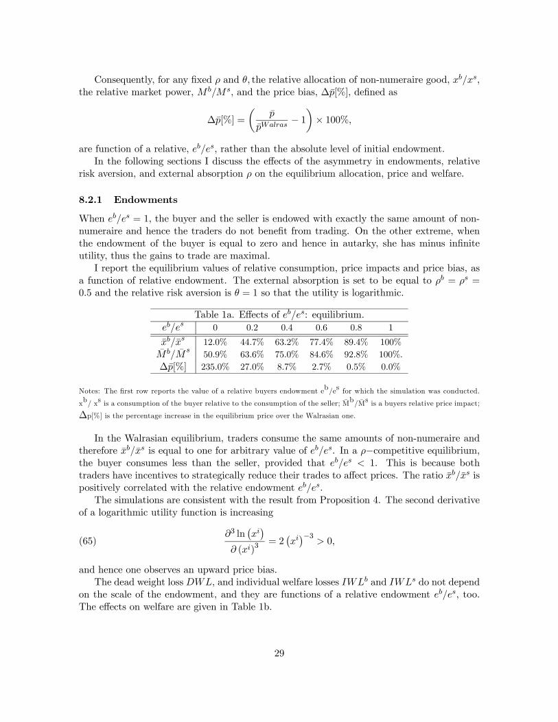
Consequently, for any fixed ρ and θ, the relative allocation of non-numeraire good, xb/xs,the relative market power, M b/Ms, and the price bias, ∆p[%], defined as

∆p[%] =

µp

pWalras− 1¶× 100%,

are function of a relative, eb/es, rather than the absolute level of initial endowment.In the following sections I discuss the effects of the asymmetry in endowments, relative

risk aversion, and external absorption ρ on the equilibrium allocation, price and welfare.

8.2.1 Endowments

When eb/es = 1, the buyer and the seller is endowed with exactly the same amount of non-numeraire and hence the traders do not benefit from trading. On the other extreme, whenthe endowment of the buyer is equal to zero and hence in autarky, she has minus infiniteutility, thus the gains to trade are maximal.

I report the equilibrium values of relative consumption, price impacts and price bias, asa function of relative endowment. The external absorption is set to be equal to ρb = ρs =0.5 and the relative risk aversion is θ = 1 so that the utility is logarithmic.

Table 1a. Effects of eb/es: equilibrium.eb/es 0 0.2 0.4 0.6 0.8 1

xb/xs 12.0% 44.7% 63.2% 77.4% 89.4% 100%M b/M

s50.9% 63.6% 75.0% 84.6% 92.8% 100%.

∆p[%] 235.0% 27.0% 8.7% 2.7% 0.5% 0.0%

Notes: The first row reports the value of a relative buyers endowment eb/es for which the simulation was conducted.

xb/ xs is a consumption of the buyer relative to the consumption of the seller; Mb/Ms is a buyers relative price impact;

∆p[%] is the percentage increase in the equilibrium price over the Walrasian one.

In the Walrasian equilibrium, traders consume the same amounts of non-numeraire andtherefore xb/xs is equal to one for arbitrary value of eb/es. In a ρ−competitive equilibrium,the buyer consumes less than the seller, provided that eb/es < 1. This is because bothtraders have incentives to strategically reduce their trades to affect prices. The ratio xb/xs ispositively correlated with the relative endowment eb/es.

The simulations are consistent with the result from Proposition 4. The second derivativeof a logarithmic utility function is increasing

(65)∂3 ln

¡xi¢

∂ (xi)3= 2

¡xi¢−3

> 0,

and hence one observes an upward price bias.The dead weight loss DWL, and individual welfare losses IWLb and IWLs do not depend

on the scale of the endowment, and they are functions of a relative endowment eb/es, too.The effects on welfare are given in Table 1b.

29

Table 1b. Effects of eb/es: welfare.eb/es18 0 0.2 0.4 0.6 0.8 1

DWL 37.9% 28.1% 25.6% 25.2% 25.0% 25.0%IWLb 42.5% 40.8% 36.4% 32.3% 28.5% 25%.IWLs -70.0% -11.8% 6.0% 15.3% 21.0% 25.0%

Notes: The first row reports the value of a relative buyers endowment eb/es for which the simulation was conducted.

DWL is an aggregate loss of welfare associated with non-competitive trade as a fraction of total gains to trade in the

economy; IWLb and IWLs are buyer’s and seller’s individual losses/gains of welfare due to a non-competitive trade as

a fraction of the individual gains to trade in a competitive equilibrium.

It can be seen that the welfare loss, as a fraction of total gains to trade, is relativelystable. It varies from −33% for the lowest relative endowment to −25% in the case whenthere are no gains to trade at all. When eb/es approaches 1, the aggregate gains to tradeare minimal and therefore in absolute terms the loss of utility is also close to zero. Thelast column suggests that when the endowments are nearly symmetric, the welfare loss isuniformly spread between the buyer and the seller: each of them is losing 25% of theirpotential gains. When endowments differ substantially, the seller is able to pass most of thewelfare cost onto the buyer. For eb/es ≤ 0.3, the seller’s benefit from being a monopoly issufficient to compensate for the welfare loss associated with the reduced volume of trade. Inthis case, the buyer not only “pays” the cost of a dead weight loss but also a monopoly rentto the seller.

8.2.2 Relative Risk Aversion

Now I examine the effects of a different level of relative risk aversion. Table 2a reportsthe numerical simulations of a 0.5−competitive equilibrium (ρi = 0.5), with the relativeendowment equal to eb/es = 40%, for the following values of relative risk aversion θ = 0.5, 1,2 and 3.

Table 2a. Effects of θ: equilibrium.θ 0.5 1 2 3

xb/xs 63.8% 63.2% 61.6% 59.5%M b/M

s80.4% 75.0% 65% 58.9%

∆p[%] 3.1% 8.7% 29.6% 69.7%

Notes: The first row reports the value of a relative risk aversion θ for which the simulation was conducted. xb/ xs is aconsumption of the buyer relative to the consumption of the seller; Mb/Ms is a buyers relative price impact; ∆p[%] isthe percentage increase in the equilibrium price over the Walrasian one.

The relative consumption xb/xs is decreasing in θ. This seems paradoxical as the moreconcave the utility functions, the greater the gains to trade. Note, however, that marketpower is increasing in the convexity of the utility functions |u00 (·)|, which in turn negatively18 In the first and last column I give the limits of the statistics, as eb/es is approaching 0 and 1 respectively,

as the statistics are not defined for the two values of relative endowment.

30

affects the trade. The relative risk aversion also magnifies the asymmetry of market power.For θ = 3, the buyer only has 58% of the sellers price impact. This in turn positively affectsthe markup over a competitive price. The effects of relative risk aversion on welfare are givenin Table 2b.

Table 2b. Effects of θ: welfare.θ 0.5 1 2 3

DWL 25.4% 25.6% 26.4% 27.9%IWLb 34.0% 36.4% 40.6% 44.1%IWLs 11.9% 6.0% -8.7% -28.3%

Notes: The first row reports the value of a relative risk aversion θ for which the simulation was conducted. DWL is

an aggregate loss of welfare associated with non-competitive trade as a fraction of total gains to trade in the economy;

IWLb and IWLs are buyer’s and seller’s individual losses/gains of welfare due to a non-competitive trade as a fraction

of the individual gains to trade in a competitive equilibrium.

The dead weight loss is only modestly increasing in relative risk aversion, but the dis-tribution of the welfare loss is very sensitive to changes in θ. For relatively small values ofθ, both traders are worse-off in a ρ−competitive equilibrium. When θ is high, the effect ofendogenous convexity implies that the majority of the aggregate welfare loss comes from thereduction of utility of the buyer. For θ greater than one, the seller extracts the utility usingits superior market power.

8.2.3 Symmetric External Absorption

In this section, I investigate the consequences of the symmetric external absorption ρb = ρs =ρ and in the following section I discuss the effects of its asymmetry. In both sections, I assumea logarithmic utility function and the value of a relative endowment equal to eb/es = 0.40%.

Table 3a gives the results for different values of ρ.

Table 3a. Effects of ρ: equilibrium.ρ 0.1 0.3 0.5 0.7 0.9 1

xb/xs 43.2% 51.8% 63.2% 76.7% 91.7% 100%M b/M

s93.0% 81.5% 75.0% 75.5% 86.9% n.d.

∆p[%] 19.4% 14.8% 8.7% 3.6% 0.5% 0.0%

Notes: The first row reports the value of the symmetric external absorption ρ for which the simulation was conducted.

xb/xs is a consumption of the buyer relative to the consumption of the seller; Mb/Ms is a buyers relative price impact;

∆p[%] is the percentage increase in the equilibrium price over the Walrasian one.

The relative consumption is increasing in ρ to a competitive level xb/xs = 100%, for ρ = 1.Surprisingly, the relative market power is decreasing in ρ. This shows that for low values ofρ, the mutual reinforcement effect of price impacts dominates the endogenous asymmetry ofthe convexity (see Proposition 4). Price bias is also negatively related to ρ.

The dead weight loss is decreasing in ρ. Interestingly, the seller is better off in aρ−competitive equilibrium provided that the external absorption is not too small. Intu-itively this is because for high values of ρ, the relative market power of the seller is high, and

31

hence she benefits from a higher price, while the trade volume is still relatively large. When ρis small, the sellers utility gains associated with higher price are not sufficient to compensatethe welfare loss due to a reduced volume of trade.

Table 3b. Effects of ρ: welfare.ρ 0.1 0.3 0.5 0.7 0.9 1

DWL 84.3% 52.3% 25.6% 8.6% 0.9% 0.0%IWLb 87.3% 61.7% 36.4% 15.5% 2.2% 0.0%IWLs 78.7% 35.3% 6.0% -3.9% -1.37% 0.0%

Notes: The first row reports the value of the symmetric external absorption ρ for which the simulation was conducted.

DWL is an aggregate loss of welfare associated with a non-competitive trade as a fraction of total gains to trade in the

economy; IWLb and IWLs are buyer’s and seller’s individual losses/gains of welfare due to a non-competitive trade as

a fraction of the individual gains to trade in a competitive equilibrium.

8.2.4 Asymmetric Bilateral Monopoly

In this section, I examine the effects of the asymmetry in external absorption. In Tables 4aand 4b, the column associated with ρb = 0 and ρs = 1 gives results for the economy with amonopolistic seller and a competitive buyer (pure monopoly). In last column, with ρb = 1and ρs = 0, the buyer has full market power while the seller is competitive (pure monopsony).The intermediate columns represent the case of bilateral monopoly with different levels ofasymmetry.

The relative consumption of the buyer xb/xs is “U” shaped. It is large for extrememonopolies and smaller for a symmetric bilateral monopoly. This is because the mutualreinforcement of price impacts is not present in a pure monopoly or monopsony and thereforethe market power is relatively low in general. In addition, the incentives to reduce thetrade are partially offset by the favorable price change for the two extremes. The relativeconsumption is greater in the case of a pure monopsony than in a monopoly. With logarithmicutility function, the buyer’s gains to trade are substantially higher than for the seller, and thebuyer is not willing to sacrifice such benefits as much as the seller does in order to decreasethe price. Not surprisingly, the price bias is negative for the pure monopsony, and positivefor the pure monopoly.

Table 4a. Effects of asymmetric ρ: equilibrium.ρs 1 0.8 0.6 0.5 0.4 0.2 0ρb 0 0.2 0.4 0.5 0.6 0.8 1

xb/xs 78.4% 69.9% 64.6% 63.2% 62.8% 64.33% 69.6%M b/M

s ∞% 197.8% 98.3% 75.0% 57.2% 28.3% 0.0%∆p [%] -10.8% -2.8% 5.1% 8.7% 12.1% 17.7% 21.8%

Notes: The first two rows report the values of external absorption for the buyers and the seller for which the simulation

was conducted. xb/xs is a consumption of the buyer relative to the consumption of the seller; M b/Msis a buyer’s

relative price impact; ∆p [%] is the percentage increase in the equilibrium price over the Walrasian one.

The pattern of aggregate welfare loss is a mirror image of the relative consumption andtherefore DWL has an inverted “U” shape. On the individual level, the buyer is better-off as

32

a pure monopsony and the seller as a pure monopoly. In general, the seller is willing to usemarket power more aggressively than the buyer as her welfare loss associated with reducedvolume of trade is smaller than the one of the buyer.

Table 4b. Effects of asymmetric ρ: welfare.ρs 1 0.8 0.6 0.5 0.4 0.2 0ρb 0 0.2 0.4 0.5 0.6 0.8 1

DWL 7.2% 15.2% 23.4% 25.6% 26.5% 23.8% 16.0%IWLb -19.2% 8.3% 29.0% 36.4% 42.1% 49.7% 55.5%IWLs 55.5% 29.3% 13.5% 6.0% -1.9% -23.6% -55.7%

Notes: The first two rows report the values of external absorption for the buyers and the seller for which the simulation

was conducted. DWL is an aggregate loss of welfare associated with non-competitive trade as a fraction of total

gains to trade in the economy; IWLb and IWLs are buyer’s and seller’s individual losses/gains of welfare, due to

a non-competitive trade as a fraction of the individual gains to trade in a competitive equilibrium.

8.3 Equilibrium with Producers: Robinson Crusoe Inc.

So far I have focused on the non-competitive interactions in a pure exchange economy. Nowto the economy from Section 8.1, I introduce production firms and demonstrate in the simpleexample how the ownership structure affects the equilibrium outcome.

I first study an economy with J incorporated firms, with technology characterized by aquadratic cost function for each good l ∈ L

(66) f jl =γl2

³yjl

´2.

The quadratic preferences of the consumers are as in equation (46), and the convexities of theutility function and the cost function, γl, coincide. The consumers’ non-numeraire endow-ments are equal to zero and the shares are distributed according to some vector θ ∈ RI×J .Throughout this section I assume the same level of external absorption for all consumers andfirms, ρil = ρjl = ρ.

As in the pure exchange economy from Section 8.1, ρ−competitive equilibrium has aclosed form solution. The equilibrium prices do not depend on the absolute number of thetraders but on the composition of the traders in the economy

(67) pl = pWalrasl =

I

I + J.

Moreover, prices are independent from the level of external absorption. The price impactsare identical for all firms and consumers and are given by

(68) M il,l = M j

l,l =1− ρl

I + J + ρl − 2γl.

They are increasing in γl, and decreasing in ρ and absolute number of traders N = I + J .Finally, the non-numeraire allocation is given by

(69) xil = til =I + J + ρl − 2I + J − 1 xi,Walras

l where xi,Walrasl =

1

γl

J

I + J,

33

and the individual stable supply is

(70) yjl = −tjl =

I + J + ρl − 2I + J − 1 yj,Walras

l where yj,Walrasl =

1

γl

I

I + J.

Consider the simplest version of the considered economy, with one non-numeraire good,one consumer, and one firm I = J = 1, and also assume γ = 1. The equilibrium in such aneconomy is depicted in Figure 7a. For ρ = 1, it coincides with a Walrasian equilibrium andis given by

(71) xi,Walras = yj,Walras =1

2, pWalras =

1

2and πWalras =

1

8.

The equilibrium allocation is Pareto efficient, therefore it can be determined as a tangencypoint of the indifference curve and the production set. The consumer’s budget set at equi-librium prices consists of all

¡ti,mi

¢below the iso—profit line πWalras. When Robinson is a

sole proprietor of the firm, then he would chose the Pareto optimal (Walrasian) allocation,regardless of the value of ρ.

Now suppose that the firm is incorporated and therefore it maximizes profit. With ex-ternal absorption strictly smaller than one, for example ρ = 0.5, a unique ρ−competitiveequilibrium is given by

(72) xi = yj =1

4, p =

1

2, M i = M j = 1 and π =

3

32< πWalras.

The stable choice of the firms is depicted in panel b). The equilibrium iso—profit parabolais tangent to a production set at

¡yj , mj

¢, and it cuts the numeraire axes at the equilibrium

profit π = 332 . The stable choice of the consumer is shown in panel c). The budget set

corresponds to the interior of the parabola that crosses the numeraire axes at π = 332 and also

passes through the equilibrium allocation¡−18 ,

14

¢. By definition of stability, the indifference

curve is tangent at¡−18 ,

14

¢to the budget set. Note, however, that the indifference curve is

not tangent to the production set, and hence the equilibrium allocation is Pareto inefficient.It should be noted that in the case of a sole proprietorship, Pareto efficiency results from

the fact that Robinson is the only trader in the economy. The sole proprietorship is notnecessarily more efficient than the incorporated ownership.

Any allocation on the frontier of the production set located between the Walrasian allo-cation

¡−14 ,

12

¢and the autarky (0, 0) can be a part of an equilibrium for some value of ρ (this

is shown in panel d). In addition, any 0−competitive allocation in the k- replica economy isalso on the frontier, between allocation

¡−16 ,

13

¢corresponding to k = 2, and the Walrasian

allocation¡−14 ,

12

¢for k approaching infinity.

With asymmetric external absorption, the geometric representation of an equilibriumdiffers from the one depicted in Figure 7 as follows: For a pure monopoly (ρj = 0, andρi = 1), the budget set of a consumer in panel c) becomes linear and in the case of a puremonopsony, (ρj = 1 and ρi = 0) the iso—profit curves in panel b) are linear.

34

ji tt −, ji tt −,

ji mm −,ji tt −,

ji mm −,

ji mm −,ji tt −,

ji mm −,

81/=Walrasπ

⎟⎠⎞

⎜⎝⎛− ,,

41

81

jY

if

323 /=π

50.=ρ1=ρ

jY

⎟⎠⎞

⎜⎝⎛

21

41 ,

π

if 0→ρ

⎟⎠⎞

⎜⎝⎛− ,,

41

81

BS

a) b)

c) d)

Figure 7. Equilibrium in the economy with a firm.

8.4 Increasing Returns to Scale and a Natural Monopoly.

Sometimes establishing a firm is associated with large fixed costs while the production ischaracterized by a constant marginal cost. In such case the average cost is monotonicallydecreasing, and the technology exhibits increasing returns to scale. I call such a firm a naturalmonopoly. The behavior of a natural monopoly cannot be studied within the Walrasianframework. This is because the firm’s competitive supply is either infinite or zero, dependingon whether the price is above the marginal cost or not. In this section, I demonstrate howthe natural monopoly can be incorporated in a general equilibrium framework when tradershave market power.

I consider an economy with one non-numeraire good, one firm characterized by the fol-lowing cost function

(73) f j¡yj¢=

½F + cyj if yj > 00 otherwise

¾,

and I consumers with a quadratic utility function given by (46). The initial endowments arenormalized to zero. In equation (73), F corresponds to a fixed cost and c is a marginal cost.The production set of the monopoly is depicted in Figure 8a. The cost function in (73) doesnot satisfy assumptions A7 and A9 and hence the considered economy is not smooth andseparable. Consequently, the theorems from Section 7 do not apply here.

When F is already a sunk cost, the production set does contain inaction point (0, 0) andhence is convex. In such case, a stable supply function can be determined from the first order

35

stability condition (35) . The equality between marginal cost and marginal revenue implies

(74) yj ≡ −tj = 1

M j(p− c) ,

for any p ≥ c and 0 otherwise. In Figure 8, the stable supply is geometrically determined asa tangency point of the iso—profit parabola and the production set.

If F is a fixed rather than a sunk cost, the inaction point is a feasible option for thefirm, and hence the production plan yj from (74) may fail to be stable. This would be thecase when yj is associated with a negative profit, and hence the natural monopoly prefers theinaction point. In Figure 8, the zero profit parabola passing through trade (0.0) is representedby a dashed line. If yj is in the interior of this parabola, it dominates the inaction point interms of profit and hence it is stable on the whole production set (see panel a). In panel b),yj is not profitable and therefore it is not stable.

a) b)

jm−F

jy

jm−

jy0=π

0=π

0>π

Figure 8. The existence of a stable supply.

The individual inverse supply function is depicted in Figure 9 in space¡yj , p

¢. The

tangency condition (74) defines a straight line originating in point (0, c) and with the slopeequal to M j .

The firm’s profit is non-negative if and only if the observed price is greater or equal tothe average cost

(75) p ≥ AC ≡ c+ F/yj ,

and therefore all combinations¡yj , p

¢below the average cost curve are associated with a

negative profit. Consequently, the stable supply function is a half line to the right of the AC

36

curve.

a) b)

jy

c

p

M

slope

jy

jy

p

( )AC MM >'

slope

( )FAC ( )'FAC

itI ⋅

Figure 9. Stable supply function of a natural monopoly and equilibrium.

The aggregate stable demand of the consumers is as in the previous section. In Figure9b, a natural candidate for a ρ−competitive equilibrium is the trade and the price for whichthe stable supply and demand intersect. Solving the model analytically reveals that at thispoint, the price is equal to

(76) p =(1 + c)

2.

The price does not depend on the number of consumers I. This is because for higher I,the larger aggregate demand is accompanied with increased supply due to the reduced priceimpact of the monopoly and the prices may stay the same.

With the possibility of inaction, the intersection point determines 0−competitive equilib-rium only if the average cost does not exceed price (76). This happens in Figure 9b for afixed cost equal to F . When, however, F 0 > F , at the price p the firm incurs a loss, thereforeit shuts down the production. In such case, an equilibrium with an active firm fails to exist.

It can be shown that for any fixed value of F ≥ 0, there exists a critical mass of consumers,I, such that in the economy with I ≥ I consumers, the equilibrium with an active monopolyexists, and with I < I it does not. Similarly, for any number of consumers, I ≥ 2, thereexists a threshold value of F , for which the equilibrium with a monopoly exists if and only ifF ≤ F . In Figure 9, threshold F can be determined as the fixed cost for which the AC locuspasses through the intersecting point of the demand and supply.

8.5 Endogenous Market Structure

In the previous sections, the number of operating firms was exogenously fixed. Here I willassume that in the considered economy, there is an infinite number of entrepreneurs whohave access to the most efficient, commonly known technology, and they may potentially useit to form a production firm. Formation of a firm is motivated by a non-numeraire profit.The technology to produce non-numeraire commodities is given by some cost function f .An economy consists of two elements: A pure exchange economy satisfying A1—A5 and atechnology f ,

(77) ELR =³¡ui, ei

¢i∈I , f

´.

37

In a Marshallian long run equilibrium, the assumptions of free entry and price taking be-havior imply that price is equal to a minimal average cost and each firm produces at the mostefficient scale. The number of active firms is determined as a ratio of the aggregate demanddivided by the individual production. This approach has the following drawbacks: The equi-librium is well defined only for the technology characterized by a “U” shaped average cost,and hence the model does not give any predictions for the industries with increasing returnsto scale. In addition, the model assumes price taking behavior by all market participantseven if the predicted number of firms is small. Finally, the assumption of “profit taking” bypotential entrants rules out the possibility of strictly positive profit in equilibrium. Here Iredefine the notion of long run equilibrium to free it from such drawbacks.

By EJ =¡u, e, θJ , f × J

¢, I denote an exchange economy with J identical firms using

technology f , and θJ is an arbitrary distribution of shares of the firms among the consumers.The ρ−competitive equilibrium in EJ is symmetric if tj is the same for all j ∈ J and firm jis active if tj 6= 0. The long run equilibrium is defined iteratively in the following way:

Definition 5 A long run equilibrium in economy ELR is a vector (p, t, M , J) such that1)¡p, t, M

¢is a symmetric 0− competitive equilibrium in E J with J active firms.

2) No profitable or profit reducing entry, that is for any J > J:a) if πJ > 0, there does not exist an 0− competitive equilibrium in economy EJ ,b) if πJ = 0 there does not exist a symmetric 0− competitive equilibrium in economy EJwith πJ > 0.

The first condition assures that none of the active firms have incentives to change thetraded quantities and all markets clear. The second condition prevents the non-active firmsfrom entering the industry. I assume that a new firm is formed if the current observed profitis strictly positive and the industry may accommodate additional firms. A firm will also beformed even if the observed profit is zero, provided that after the entry in a new equilibriumthe profit is positive. Observe that there are no incentives to entry when the current observedprofit and the profit after entry is zero.

By Theorem 1, there exists a 0−competitive equilibrium in a pure exchange economywith J = 0, provided I > 2. Such equilibrium is not a long run equilibrium only if thereexists a 0−competitive equilibrium in the economy EJ for some J > 0, with firms makinga positive profit. This in turn is not a long run equilibrium only if there is an equilibriumin the economy with J 0 > J firms. This shows that the long run equilibrium exists or theeconomy can accommodate an arbitrarily large number of firms, all making a strictly positiveprofit. With many firms the price impact is negligible, therefore the economies without longrun equilibrium are called competitive.

In the following sections I verify what market structures are compatible with differenttypes of technology.

8.5.1 Natural Monopoly

The active or inactive monopoly studied in Section 8.4 is the only market structure compatiblewith the cost function given by (73). This is because with two or more operating firms,

38

constant marginal cost makes positive price impacts inconsistent with off-equilibrium marketclearing condition19.

Lemma 2 Suppose the second derivative of the cost function is equal to zero, f 00 (·) = 0.In a symmetric 0−competitive equilibrium, the price impacts Mn > 0 are consistent withoff-equilibrium market clearing condition if and only if J = 1.

Intuitively, with the price impact of firm j equal to M j > 0, and without extra convexity“added” by the Hessian of the cost function D2f j = 0, any unilateral deviation by firm j0 isfollowed by the response of firm j sufficient to make the price impact of j0 only a fraction ofM j . Because firms are symmetric, this is possible only if M j = M j0 = 0.

Strictly positive price impacts M j > 0 are necessary for the existence of a stable supplyfunction given the cost function (73). Hence there does not exist a ρ−competitive equilibriumwith J ≥ 2, and the monopoly is the richest market structure compatible with such a costfunction. Intuitively, new firms are not willing to challenge the natural monopoly as theirentry triggers perfectly competitive interactions resulting in strictly negative profits for allfirms.

8.5.2 Perfectly Competitive Oligopoly

For the cost function

(78) f j¡yj¢= cyj ,

associated with constant returns to scale, the model predicts oligopolistic market structure,including a duopoly. The equilibrium price is equal to a marginal cost, p = c, and the profitequal to zero, πj = 0. This is because with constant marginal cost and J ≥ 2, Lemma 2implies that the positive price impact M j > 0 is inconsistent with ρ−competitive equilibrium.For M j = 0, the stable supply of the oligopolistic firm is well defined, and it coincides withthe Walrasian supply

(79) yj ≡ −tj =

⎧⎨⎩0 if p < c

0 ≤ yj ≤ ∞ for p = c∞ otherwise

⎫⎬⎭ .

With such supply function, any unilateral deviation of a trader is absorbed by other activeoligopolists without any effect on price. Consequently, Mn = 0 for all traders n = i, j isconsistent with off-equilibrium market clearing. The number of firms and the individual levelof production is not determined by the model. In fact, any J ≥ 2 and tj satisfying

(80) tj =

Pi∈I t

i (c, 0)

J> 0

is consistent with equilibrium. Observe that such equilibrium is Pareto efficient.A monopoly with constant returns to scale will not be observed in equilibrium. The

monopolistic firm is trading with consumers, and hence it faces a downward sloping demand,19This result is consistent with the findings of Bresnahan [1981], in Example 6 for a duopoly and Perry

[1983] Section 3 for oligopoly.

39

and hence has strictly positive profit. This in turn encourages other firms to enter theindustry. By a similar argument, the economy with J = 0 is not a long run equilibriumbecause with J = 1 the firm makes a strictly positive profit, as long as

Pi∈I t

i (c, 0) > 0, andhence there are incentives to form a monopoly.

8.5.3 Imperfectly Competitive Oligopoly

In the following two sections, I focus on strictly convex cost functions. First I consider a costfunction with a positive fixed cost that is given by

(81) f¡yj¢=

½F + c

¡yj¢if yj > 0

0 otherwise

¾.

c¡yj¢is strictly increasing, strictly convex and marginal cost satisfies c0 (0) = 0.

The average cost is either monotonically decreasing and hence the technology exhibitsincreasing returns to scale20, or the average cost has a “U” shape and has a well definedminimal efficient scale. In the long run, such technology induces a monopolistic or oligopolisticmarket structure in which active firms have positive price impacts and typically positiveprofits.

Market structure with “U” shaped average cost was extensively studied within the com-petitive framework. For example, with quadratic cost function

(82) f¡yj¢=

½F + γ

2

¡yj¢2 if yj > 0

0 otherwise

¾,

the competitive long run equilibrium predicts that each firm produces at the minimal efficientscale, and price is equal to a minimal average cost,

(83) yj =

s2F

γ, p =

p2F γ.

The number of consumers per each firm can be found as a ratio of the level of productionof a typical firm and the demand of each consumer. With I consumers characterized by aquadratic utility functions

(84) U¡xi,mj

¢= αxi − γ

2

¡xi¢2+mi,

this ratio is equal to

(85)I

J=

√2Fγ

αi −√2Fγ

.

The ratio is independent from the absolute scale of the economy.20The example of the cost function that is strictly increasing, strictly convex and with monotonically de-

creasing average cost is

f³yj´= F + 1 + yj − yj

yj + 1.

40

As argued before, the concept of competitive long run equilibrium is not coherent unlessthe economy is large. With the relatively small number of active firms, the price and profittaking behavior is not justified. In addition, with only a few consumers, one should alsoexpect some monopsony power on the buyer’s side.

Using the framework from this paper, I find the magnitude of the small scale biases in thepredictions of the competitive long run equilibrium in the economy with consumers’ utilityfunction given by (84) and technology (82) . Table 5 summarizes the results for the followingvalues of parameters F = 10, γ = 10 and α = 15.

Table 5. Small scale correction.J 1 2 3 10 100 Walras

I 18-33 34-49 50-66 165-181 1649-1665 1-∞I/J 18-33 17-24.5 16.66-22.0 16.5-18.1 16.48-16.65 16.48y 1.34-1.41 1.38-1.41 1.38-1.41 1.406-1.413 1.413-14.14 1.414y 14.21-14.56 14.17-14.41 14.15-14.35 14.134-14.215 14.142-14.15 14.142π 0.07-0.59 0.026-0.380 0.008-0.290 0.00-0.103 0.00-0.011 0

Notes: The first row, J reports the number of firms in the industry for which the simulation was conducted. I is

the number of consumers compatible with J firms; I/J is the number of consumers per firm. y gives the range of

production levels; p denotes a price and π is profit.

The first row denoted by J , defines the market structure in question. For example, columnJ = 1 represents a monopoly, J = 2, is a duopoly and for J > 2 it is an oligopoly with J firms.In the column “Walras” I report the predictions of the competitive long run equilibrium. RowI gives the the numbers of consumers supporting considered market structure, and row I/Jinforms about the number of consumers per each active firm. The last three rows give thelevel of firms production, equilibrium price and profit.

It can be seen that the profits of the oligopolistic firms are positive and the price is abovethe minimal average cost. In the small economy, the number of consumers per active firmis significantly above the value predicted by the Walrasian equilibrium. For example, themonopoly serves from 18 to 33 consumers and not the predicted 16.48. One of the reasonsfor this is that indivisibility of a fixed cost prevents the other firms from entering the industry,even if the incumbent has a relatively high profit. In addition, in a small economy, consumershave some market power and hence the aggregate demand is below the competitive one. Onthe other hand, the simulations suggest that the Walrasian long run equilibrium is a goodapproximation when the number of operating firms is large. In the economy with more thanone hundred active firms, the gap in the predictions of the two frameworks becomes negligible.

8.5.4 Competitive Economy

When in the cost function given by (81) the value of fixed cost is zero, F = 0, the longrun equilibrium fails to exist. For any value of J, Theorem 1 asserts that one can find aρ−competitive one. It is easy to show that given identical cost function, all firms producethe same amount of output and hence the equilibrium is symmetric, and with increasingmarginal cost all firms make a positive profit. Hence for any J there are always incentives toform new firms. By definition, the economy without the long run equilibrium is competitive.

41

9 Determinants of Market Power and Policy Implications

The key to understanding the phenomenon of market power is a source of trader’s priceimpact defined as her ability to affect prices by marginally changing her trade. The presentedframework gives some insights into the nature of determinants of price impacts, a phenomenonlong ignored in the economic literature.

9.1 Determinants of Price Impacts

The essential ingredient of a price impact of each trader is a convexity of utility (negative ofthe second derivative) or cost functions of the trading partners. The steeper the marginalutility or cost of the other traders, the greater the price change needed to make others willingto absorb the off-equilibrium deviation. Therefore the trader with the highest convexity hasthe lowest price impacts, as she trades with a group of traders characterized by the lowestconvexity. More generally, the traders’ ranking with respect to the strength of price impactis a reversed order of their convexities.

Some economies endogenously assign higher market power to sellers than to buyers. Forexample, this is the case in a pure exchange economy with identical utility functions with apositive third derivative. In equilibrium, the convexities of buyers are naturally above thesellers’ and hence sellers have more substantial price impacts.

Price impacts are subject to a mutual reinforcement effect. They “add” to the convexi-ties of utility or cost functions, making the traders more reluctant to absorb the unilateraldeviations of other traders. This positively affects price impacts of the remaining traders.The mutual reinforcement effect amplifies the overall level of price impact in the economy.

It does not matter for the price impact whether the trader is a firm maximizing profitor a consumer. In equilibrium, consumers and firms with the same convexity have identicalprice impacts.

Surprisingly, price impact does not depend on the trader’s share in the total volume oftrade. Even if one of the traders is a sole supplier of a commodity on the market, she hasthe same price impact as others, provided that the convexities are the same.

Price impacts are always decreasing in the absolute number of traders. Note that this isnot necessarily the case in the model of Cournot. With a linear demand function, the Cournotmodel predicts/assumes that the price impact of an oligopolist is the same, regardless of thenumber of firms operating in the industry and it is equal to the slope of a demand of theindustry. This is because in the Nash equilibrium, strategic traders do not react to unilateraloff-equilibrium deviations, and the price impacts are solely determined by the reaction ofcompetitive consumers.

In the economic literature, market power is associated with large traders. This is becausethe same price impact affects traders’ decisions in a different way, depending on her volumeof trade. For example, with the price impact and the supply equal to one, the producer,by selling additional unit of a good, is losing only one dollar on the previous sales due to areduced price. When the original volume of trade is equal to one hundred units, the loss ofprofit amounts to one hundred dollars. Consequently, large traders are affected more severelythan the smaller ones, and hence their non-competitive behavior is more pronounced. Inother words, what matters is the elasticity of the demand function, and price impact is only

42

one of its components.Finally, I would like to stress the role of a harmonic mean in the framework. The consis-

tency condition on price impacts implies that a trader’s price impact is equal to a harmonicmean of price impacts and convexities of utility or cost functions of the remaining traders,

(86) Mn =1

N − 1H¡Mn + V n|n0 6= n

¢,

and multiplied by a discount factor 1/ (N − 1). Harmonic mean arises naturally in the con-sistency condition as it puts higher weight on the traders with smaller convexities. Observethat such traders absorb most of the unilateral deviation and hence are key in price impactdetermination. The traders with almost linear utility or cost functions are willing to absorboff-equilibrium deviation without any price reward, making price impacts of other tradersnegligible. This corresponds to the property of the harmonic mean that whenever one of itselements converges to zero, the value of the mean also becomes zero.

9.2 Mergers and Antitrust Policy

The analytical framework used by the Department of Justice and the Federal Trade Com-mission to determine whether mergers are likely to lessen the competition of the industryis primarily based on the Herfindahl-Hirschman Index (HHI). HHI measures post-mergermarket concentration by summing the squares of the market shares of all market participants.

(87) HHI =Xj∈J

¡sj¢2,

where sj is a share in the sales on the market by firm j. Markets with HHI above 1800 areconsidered highly concentrated, and mergers increasing HHI by more than 100 points areassumed to be likely to “create or enhance market power or facilitate its exercise.”

The model presented in this paper suggests that HHI does not contain sufficient informa-tion for the evaluation of the unilateral21 effects of mergers on competitiveness of the market.This is because, other things being equal, oligopolistic market power critically depends onthe convexity of the cost functions of the other firms. In the industries characterized by largefixed costs and approximately constant marginal costs, the interactions should be competitiveeven if the number of firms is small. Consider a software industry with three firms of equalsize, and suppose that two of them are considering a merger to save on fixed costs. The postmerger Herfindahl-Hirschman index is equal to

(88) HHI = 5445,

so the market is considered as highly concentrated. In addition, the merger increases HHIby 2178, and therefore the merger is likely to be blocked. If, however, the marginal cost isconstant, such a merger does not enhance market power at all! In addition, with increasingreturns to scale such a merger is Pareto improving, as it reduces the fixed cost expenses.

21The model by assumption rules out the merger effects on lessening the competition through a coordinatedinteraction.

43

10 Relation to Other Non-competitive Models

When external absorption is equal to one for all traders, the framework becomes the Walrasianone. In this section, I argue that several other non-competitive models of market interactionsare also embedded in the proposed framework.

10.1 Unilateral Monopoly, Dixit-Stiglitz Monopolistic Competition

The models of unilateral monopoly assume that only one trader in each market has marketpower. An example of such models include a standard monopoly or monopsony. Such modelshave been extensively studied in economic literature.

Technically, the models of a unilateral monopoly can be obtained within the proposedframework by setting the value of external absorption of one trader to zero, and for theremaining traders to one. For example, in the economy with one consumer and one firm,setting ρi = 1 for the consumer and ρj = 0 for the producer transforms the framework intoa standard model of monopoly. When the values are reverted, i.e., ρi = 0 and ρj = 1, itbecomes a model of monopsony. The proper values of external absorption for a buyer and aseller in the Edgeworth box economy define a model of monopoly or monopsony.

The most prominent example of a unilateral monopoly is a model of monopolistic com-petition proposed by Dixit and Stiglitz [1977]. Dixit and Stiglitz consider an economy withone competitive consumer and J firms, each producing one non-numeraire good. Their rep-resentative consumer has preferences given by a utility function

(89) U

⎛⎝m,

ÃXl

(xl)s−1s

! ss−1⎞⎠ .

U (·, ·) is a homogenous, strictly quasi-concave and increasing function and s ∈ (1,∞). Suchpreferences are more general than the ones assumed in this paper, as they allow for differentvalues of marginal rate of substitution between money and “utility” from non-numerairegoods. I will argue, however, that in deriving their equilibrium, Dixit and Stiglitz implicitlyassumed a constant marginal rate of substitution on the individual level (the marginal rateof substitution is determined on the aggregate level).

If one defines a modified utility function as U (m,u) ≡ U³m,u

s−1s

´, the utility function

(90) U

Ãm,Xl

(xl)s−1s

!

represents the same preferences as the one in (89), and its non-numeraire argument is ad-ditively separable. The aggregate price index p and an index of aggregate non-numeraireconsumption x in the economy is defined as

(91) p =

ÃXl

(pl)1−s! 1

1−s

and x =

ÃXl

(xl)s−1s

! ss−1

.

44

The maximization of the utility function on a budget set,

(92) m+Xl

plxl ≤ I,

yields the following optimal non-numeraire demand of each l:

(93) xl =

µ1

pl

¶s

xps.

(93) and the budget constraint in (92) determine the consumption of numeraire. In generalit is very hard to find a closed form solution for the system of L + 1 non-linear equationsand L + 1 unknowns. Dixit and Stiglitz argue, however, that when the number of non-numeraire goods is large, the change of an individual price should have a negligible effect onthe aggregate price level p and also on the aggregate consumption x. They conclude that theelasticity of the demand for individual good should be approximately equal to s.

It is immediate to show that in optimum, the marginal rate of substitution between anumeraire and non-numeraire utility is equal to

(94)Um (·)Ux (·)

=s− 1s

(xps)−1s .

Therefore, fixing the value of xps is equivalent to making Um/Ux constant, too. In otherwords, Dixit and Stiglitz assume that from the perspective of an individual firm, the repre-sentative consumer behaves as if she had a quasi-linear utility function, additively separablewith respect to non-numeraire goods

U

Ãm,Xl

(xl)s−1s

!=³Um/Ux

´m+

Xl

(xl)s−1s .

Such a utility functional satisfies the assumptions A1-A5 in this paper.To close the model, Dixit and Stiglitz endogenize Um/Ux on the aggregate level. The

unique equilibrium value of Um/Ux, and the production level xl is determined22 by the con-dition that the consumers’ demand is sufficiently large to insure that the firm breaks even,given the elasticity of the demand equal to s and fixed cost equal to F . The number of goodsproduced in the economy, L, is then determined to make the equilibrium marginal rate ofsubstitution Um/Ux to be a true one. Formally, L is implicitly defined by the condition

(95)Um

¡m,Lxγl

¢Ux

¡m,Lxγl

¢ = Um

Ux

.

It is straightforward to generalize the framework in this paper to allow for the preferencesas in the monopolistic competition model of Dixit and Stiglitz. The derivation of an equi-librium requires some approximations, and therefore such a generalization come at the costof not perfect internal consistency. In this paper, I focus on the interdependencies of marketpower among traders rather than income effects in non-competitive trading. Therefore, Ileave such an extension for future research.22 In the version of monopolistic competition with a fixed number of operating firms, the marginal rate of

substitution is determined as a solution to the system of two equations and two unknowns (93), with MRS

substituted from (94), giving xl³Um/Ux

´and Um (m,xl) /Ux (m,xl).

45

10.2 Bilateral/Multilateral Monopoly, Game-theoretic Approach.

Modelling a bilateral monopoly is more complicated than the unilateral one. The complicationresults from the fact that the price impact of the oligopolist depends on the behavior andhence the price impact of the other oligopolist and vice versa. Such mutual interdependence ofprice impacts is explicitly studied in this paper. The game theoretic models solve the problemin an alternative way. They cut the link between the price impacts of different traders byimposing the condition that only price takers react to unilateral deviation of strategic players.For example, this is the case in the Cournot model.

In the Cournot model, each firm is maximizing a profit, given a demand of the industry

(96) p³yj +

Xyj´.

If the demand is determined by a market clearing condition, as in the monopolistic compe-tition studied by Gabszewicz and Vial [1972], function p () is implicitly determined by themarket clearing condition

(97)X

ti,Walras (p) = yj +Xj06=j

yj0,

which, given the inelastic supply function, yj = −tj , can be written as

(98) tj +Xj06=j

tj0 +X

ti (p, 0) = 0.

This shows that the allocation in a Cournot-Nash equilibrium is numerically equivalent to aρ−competitive equilibrium, in which external absorption of the consumers is set to one andthe firms’ off-equilibrium market clearing condition is modified so that the firms do not reactto unilateral deviations (98).

The Bertrand model can also be embedded in the framework with modified off-equilibriumprice. The Bertrand firms, however, instead of optimally responding to changes in the de-mands, are assumed to supply any demanded quantity of the good at the equilibrium price.In other words, in Nash equilibrium their trade correspondence is “flat” and defined as

(99) tj0 ¡p, M

¢=©0 ≥ −tj ≥ ∞ for p = p

ª.

With such supply correspondences with “zero” slopes, the off-equilibrium market clearingcondition predicts zero price impacts of all traders–any unilateral deviation is absorbedby the other traders without any price change. The similar reasoning generalizes to theGrossman’s model of Nash in Supply Function from Grossman [1981].

Another well-known model of a bilateral monopoly, the Shapley and Shubik strategicmarket game, cannot be mapped into the proposed framework. The reason is that in such agame, none of the traders responds optimally to changing prices after a unilateral deviation.

The framework is most closely related to the models studied by Bresnahan [1981], Perry[1982] or Hart [1985]. The key difference is that here traders here have conjectures about thedeviations of prices as a function of off-equilibrium deviations rather that the absolute levelof trade, and they make consistent conjectures not about a best response of the other player,but about the equilibrium in an economic system with many heterogenous traders.

46

11 Perfect Conjectural Equilibrium

A ρ−competitive equilibrium from this paper is an example of a Perfect Conjectural Equi-librium, a solution concept formulated in Weretka [2005c]. to moddel strategic interactionsin complex systems in which players have a possibily to revise their strategies and the onlyinformation about their environment is limited to the observations of variables relevant intheir payofs that comes from their experimentation. Each player forms believes of how sheaffects the behavior of other players ∆s−i (∆si) and take into account when reacting in andout of equilibirum.

12 Non-competitive Second Welfare Theorem

Theorem 3 asserts that the equilibrium allocation is typically Pareto inefficient. It is naturalto ask whether it is possible to design a tax system that corrects the incentives, so that Paretoefficient allocation is implementable as a ρ−competitive equilibrium.

Consider a smooth tax rule, T =¡T 1, T 2 . . . , T I , . . . , TN

¢, defined as a vector ofN smooth

functions, each specifying a tax obligation of trader n in terms of numeraire for any possiblevalue of trade tn. I restrict attention to separable tax rules, that is the rules for whichHessians D2Tn are diagonal .

By tPE I denote a unique Pareto efficient trade23. In a smooth and separable economy,tPE must satisfy

(100) Dui|tiPE = Df j |tjPE

for any i, j ∈ N . The condition (100) and market clearing is sufficient for Pareto optimalityof tPE.

With a smooth tax rule T (·), the necessary condition for stability of consumer’s trade is

(101) Dui¡ti + ei

¢= p+Ψi,

where Ψi is a distortion associated with a non-competitive trading and taxation. For anyproducer j, in the equation (101) marginal utility is replaced with the marginal cost. Thedistortion can be written as

(102) Ψn = MnT t

n +DTn.

Since in equilibrium markets clear, to implement the Pareto efficient allocation, it is sufficientto make Ψn equal across all traders n, at tPE . I focus on tax rules for which the distortionis null, Ψn = 0.

A tax rule affects Ψn in two ways. Its gradient enters equation (102) directly, changingthe first order incentives. In addition, taxes determine the price impacts of all traders inequilibrium, MT (hence M has subscript T ). Does there exist a smooth tax rule for whichtwo effects offset and hence Ψn = 0? To make the argument more transparent, I introducethe following notation: T 0n ≡ DTn (tnPE) is a gradient of a tax rule at the Pareto efficient

23 In a smooth and separable economy, there is a unique allocation x satisfying this condition. Therefore,this will also be an allocation in a unique Walrasian Equilibrium.

47

allocation and T 00i ≡ D2T i¡tiPE

¢is the Hessian. T 0, and T 00 give T 0n and T 00n for all traders.

The next proposition establishes the existence of a tax rule implementing the Pareto efficientallocation in a ρ−competitive equilibrium:

Proposition 5 Consider T 00 such that −D2ui () >> T 00i for any consumer i ∈ I andD2f j () >> T 00j for any producer j ∈ J . Then there exists a unique T 0, such that Ψn = 0for all n.

One of the implications of Proposition 5 is that for any T 00 one can find a gradient T 0

that makes the distortion equal to zero. Consequently, the proposition implies the existenceof a whole class of tax rules T implementing a Pareto efficient allocation in ρ−competitiveequilibrium. In Proposition 5 the restrictions on T 00 guarantee that the maximization problemof each trader is convex and hence first order stability conditions are sufficient. It should bestressed that it is sufficient for the result that the taxes are paid by at least two of the tradersin the economy and not all traders.

The next result demonstrates that the distortion related to non-competitive trading canbe made arbitrarily small by choosing a tax rule with Hessians sufficiently close to Hessiansof corresponding utility or cost functions.

Proposition 6 Let {Tk}k∈{1,2,...∞} be a sequence of tax rules that satisfy the assumptions ofProposition 5 and for each consumer are such that

(103) limk→∞

T 00ik = D2ui¡tiPE + ei

¢,

and for a firm

(104) limk→∞

T 00jk = −D2f j (−tPE) ,

then for each trader

(105) limk→∞

¡Mn

Tk

¢tn = 0.

Proposition 6 shows that it is possible to implement Pareto efficient allocation almostwithout affecting the first-order incentives by de-convexifying the optimization problem ofeach trader around Pareto efficient trade tnPE. The example of the sequence of tax rules from6 is

T i,k¡ti¢=

µk − 1k

¶¡ti − tiPE

¢T ¡D2ui

¡tiPE + ei

¢¢ ¡ti − tiPE

¢,(106)

T j,k¡tj¢= −

µk − 1k

¶³tj − tjPE

´T ³D2f j

³tjPE

´´³tj − tjPE

´.

Note that such a sequence satisfies the restriction on Hessians from Proposition 6. SinceD2ui

¡tiPE + ei

¢is negative definite and D2f j

³−tjPE

´is positive definite, the maximal tax

obligation is associated with trade tnPE , and it is equal to zero. For all other trades, tn 6= tnPE ,

the value of the tax is negative. In other words, trader n is paid to deviate from the Pareto

48

efficient allocation. Why is tPE implemented in a ρ−competitive equilibrium by a tax rulethat gives second-order incentives to deviate from it? Intuitively, the tax rule T k makes themarginal utility or cost nearly constant around tn

0PE for all other traders n

0. Therefore for anyunilateral deviation by n, the remaining traders are willing to take the deviation out of themarket without any change in price and hence market power of n is zero. Since this is truefor all traders, the distortion associated with market power disappears and the equilibriumbecomes competitive.

13 Conclusions

In this paper, I propose a framework for studying the outcomes of market interactions andthe determinants of market power in an economy with a small number of traders or withheterogenous traders. I study economies with consumers characterized by separable utilityfunction and firms, using a numeraire as the only input. Though these separability assump-tion are strong, the model has important applications. For example, when modeling tradeunder uncertainty, the traders are often assumed to maximize expected utility–a utilityfunction that is separable with respect to consumption in different states of the world. Thismodel also makes it possible to study phenomena associated with non-competitive trading offirms that do not depend on cross-market effects.

The assumption of separability is relaxed in Weretka[2005a]. There I study phenomena as-sociated with strategic pricing across markets. In particular, I investigate cross-subsidizationof markets and substitution of inputs traded in noncompetitive markets by competitive in-puts. I also discuss the problem of existence of equilibrium, determinacy and testability in anon-separable economy.

A vast empirical literature suggests that the trades of large institutional investors doimpact asset prices and hence returns, and that investors take this impact into account whentrading. Yet the existing models of equilibrium asset pricing assume that all investors are“return takers.” In Weretka [2005b], I use the abstract framework of non-competitive tradingto explain the effect of institutional trading on asset prices and allocations. I discuss the effectsof non-competitive trading in a model with mean-variance optimizing traders in a strategicversion of CAPM (S-CAPM). I also show that market power may account for the equitypremium and the risk-free interest rate puzzles when the utility functions are characterizedby prudence.

In [2005c], I formulate a concept of perfect conjectural equilibrium in an abstract non-cooperative smooth game, possibly with more than two heterogenous players. Intuitively, insuch a game any marginal off-equilibrium deviation of player i triggers a game among allremaining players, and the equilibrium outcome of this game is predicted correctly by playeri. When playing the game, other players are assumed to take into account their impacts onthe strategies of the other players. I study the properties of such equilibria.

References

[1] Arrow, K.J., and Hahn, F.H., (1971), General Competitive Analysis, Holden Day

49

[2] Bowley, A.L., (1924), The Mathematical Groundwork of Economics, Oxford Univer-sity Press, Oxford

[3] Boyer, M., and Moreaux, M., (1983a), Consistent versus Non-Consistent Conjec-tures in Duopoly Theory: Some Examples, Journal of Industrial Economics, 32(1), pp.97-110

[4] Boyer, M., and Moreaux, M., (1983b), Conjectures Rationality and Duopoly The-ory, Intl. Journal of Industrial Organization 1, pp. 23-41

[5] Bresnahan, T.F., (1981), Duopoly Models with Consistent Conjectures, AmericanEconomic Review, 71(5), pp. 934-945

[6] Bresnahan, T.F., (1983), Existence of Consistent Conjectures: Reply, American Eco-nomic Review, 73, pp. 457-458

[7] Chan, K.C., and Lakonishok J., (1993) Institutional Traders and Intra-day StockPrice Behavior Journal of Financial Economics, 33, pp. 173-199

[8] Chan, K.C., and Lakonishok, J., (1995) The Behavior of Stock Price Around Insti-tutional Trades Journal of Finance, 50, pp. 1147-1174

[9] Dixit, K., and Stiglitz J.E., (1977), Monopolistic Competition and Optimum Prod-uct Diversity, American Economic Review, 67 (3), pp. 297-308

[10] Frish, R., (1951), Monopoly, Polypoly. The concept of force in the economy, Interna-tional Economic Papers, 1, pp. 23-36

[11] Figueieres, C., Jean-Marie A., Quirou N., Tidball M., (2004), Theory of Con-jectural Variation, Series on Mathematical Economics and Game Theory Vol. 2, WorldScientific.

[12] Holthousen, R., Leftwich, R., and Mayers, D., (1987) The Effects of Large BlockTransations The Speed of Response and Temporary and Permanent Stock-Price Effects,Journal of Financial Economics 26, pp. 71-95 ol 2., World Scientific Publishing

[13] Gabszewicz, J.J., and Vial, J.P., (1972), Oligopoly “A la Cournot” in a GeneralEquilibrium Framework, Journal of Economic Theory, 4, pp. 381-400

[14] Gantmacher, F.R., (2000), The Theory of Matrices, Providence, RI: AMS Chelsea

[15] Grossman, S., (1981), Nash Equilibrium and the Industrial Organization of Marketswith Large Fixed Costs, Econometrica, 49, pp.1149-1172

[16] Hahn, F.H., (1978), On Non-Walrasian Equilibria, Review of Economics Studies, 45(1), pp.1-17

[17] Hahn, F.H., (1977), Exercises in Conjectural Equilibria, Scandinavian Journal of Eco-nomics, 79(2), pp. 210-26

50

[18] Hart, O., (1979), Monopolistic Competition in a Large Economy with DifferentiatedCommodities, Review of Economics Studies, 46 (1), pp. 1-30

[19] Hart, O., (1982), Reasonable Conjectures, mimeo London School of Economics

[20] Hausman, J.A., Lo J., and McKinlay, C.A., (1992) An Ordered Probit Analysis ofTransaction Stock Prices, Journal of Financial Economics, 31, pp. 319-397

[21] Holthousen, R., Leftwich R., and Mayers, D., (1987) The Effects of Large BlockTransations on Security Prices: A Cross Sectional Analysies, Journal of Financial Eco-nomics 19, pp. 237-267

[22] Holthousen, R., Leftwich R., and Mayers, D., (1990) Large Block TransationsThe Speed of Response and Temporary and Permanent Stock-Price Effects, Journal ofFinancial Economics 26, pp. 71-95.

[23] Kamien, M., and Schwartz, N., (1983), Conjectural Variation, Canadian Journal ofEconomics, 16(2), pp.192-211

[24] Keim, D.B., and Madhavan, A., (1996) The Upstairs Markets for Large-Block Tran-sations. Analisis and Meassurement of Price Effects Review of Financial Studies 9, pp.1-39

[25] Klemperer, P., and Meyer, M.A., (1989), Supply Function Equilibria in Oligopolyunder Uncertainty, Econometrica, 57, pp. 1243-1277

[26] Kraus, A., and Stoll, H., (1972) Price impact on block trading on the New YorkStock Exchange, Journal of Finance 27, pp. 569-588

[27] Laitner, J., (1980), “Rational” Duopoly Equilibria, Quarterly Journal of Economics,95(4), pp. 641-662

[28] Negishi, T., (1960), Monopolistic Competition and General Equilibrium, Review ofEconomics Studies, 28 (3), pp.196-201

[29] Perry, M., (1982), Oligopoly and Consistent Conjectural Variation, Bell Journal ofEconomics, 13, pp. 197-205

[30] Roberts, J., and Sonnenschein, H., (1977), On the Foundations of the Theory ofMonopolistic Competition, Econometrica, 45, pp.101-113

[31] Robson, A., (1983), Existence of Consistent Conjectures: Comment American Eco-nomic Review, 73, pp. 454-456

[32] Shapley, L., and Shubik, M., (1977), Trade Using One Commodity as a Means ofPayments, Journal of Political Economy, 85(5), pp. 937-968

[33] Triffin, R., (1940), Monopolistic Competition an General Equilibrium Theory, Har-vard University Press, Cambridge, Mass.

51

[34] Weretka, M., (2005a), Perfect Conjectural Equilibrium and Endogenous MarketPower: a Non-separable Case, mimeo Yale University

[35] Weretka, M., (2005b), The Institutional Traders and Non-competitive Financial Mar-kets, mimeo Yale University

[36] Weretka, M., (2005c), Perfect Conjectural Equilibria in Games, mimeo Yale Univer-sity

14 Appendix

Proof. (Proposition 1: Existence and uniqueness of a stable trade for a con-sumer.)

Consider a trade that maximizes preferences U i¡ti + ei,mi

¢on a budget set B

¡p, ti, M i

¢,

and is feasible ti + ei ≥ 0. Formally, such¡ti,mi

¢is a solution to the program

(107) maxti,mi

U¡ti + ei,mi

¢,

subject to ¡ti,mi

¢∈ B

¡p, ti, M i

¢and ti ≥ −ei.

U (·) is strictly concave in ti, and constraints are convex, provided that M i is positive definite.In addition, by strict monotonicity of preferences (in money), in optimum budget constraintwill be satisfied with equality. With symmetric M i, the necessary Khun — Tucker conditionof optimality is given by

(108)Dui − p− M i(2ti − ti) ≤ 0,pp,ti,Mi

¡ti¢· ti +mi = 0,

p(p,ti,Mi)¡ti¢= p+ M i

¡ti − ti

¢,

where the first inequality holds with equality for all commodities such that til > −eil. By thedefinition of a stable trade, ti is optimal on a budget set generated by itself and therefore theadditional necessary stability condition is

(109) ti = ti.

Equation (109) allows me to reduce (108) to

Dui − M iti ≤ p,(110)

mi + p · t = 0.

The inequality asserts that at the stable trade, marginal utility can be at most equal tomarginal revenue. For any positive definite, diagonal matrix M i, equation (110) has a uniquesolution ti. To see it observe that the first group of inequalities in (110) forms a system ofL independent inequalities, each just in one unknown. Each diagonal element is M i

l,l > 0,therefore the left hand side is decreasing in til. This function attains its maximal value,preservationl , at til = −ei and is equal to zero for some finite value of til. Therefore, for any pl

52

in the interval [0, preservationl ], there exists a unique positive value of til that solves inequality(110) with equality, and for pl in

¡preservationl ,∞

¢, the unique value of ti satisfying (110) is

zero. Given ti that solves all inequalities (110), a unique stable mi is determined by the lastequality (110). This shows that for any p ≥ 0 and positive definite M i diagonal matrix, thereexists a unique ti that is stable.

Proof. (Corollary 1: Stable trade function is differentiable in p.).Proposition 1 asserts that for any positive definite diagonal matrix M i and a price vector

p such that p ≥ 0, there exists a unique stable trade ti. This defines a function ti¡p, M i

¢. In

addition, when ti >> −ei, non-numeraire stable demand is implicitly defined by the equalityof the marginal utility and the marginal revenue (see (110))

(111) Dui¡ti + ei

¢= p+ M iti .

The derivative of the implicit function with respect to ti is given by

(112) M i −D2ui (·) .

By assumption, −D2ui (·) and M i are positive definite, therefore matrix (112) has full rank.The implicit function theorem says that in the neighborhood of p, a stable trade function,t∗i¡p, M i

¢, solving equation(110) is differentiable. Since this holds for any interior trade,

ti¡p, M i

¢is smooth for all interior trades. The implicit function theorem implies that the

derivative of the trade with respect to price

(113) D2pt¡p, M i

¢= −

¡M i −D2ui

¢−1is an inverse of the Hessian and the price impact matrix.

Proof. (Proposition 2: Existence of a differentiable, stable trade function for afirm.)

Consider a problem of a firm choosing a trade tj to maximize a profit

(114) maxti,mj

π = −¡pp,tj ,Mj

¡tj¢· tj +mj

¢,

and is constrained by the production set determined by:

(115) mj ≥ f j¡−tj

¢and tj ≤ 0.

With positive definite M j price impact matrix, the objective function is strictly concave.With M j symmetric, the necessary conditions for tj to be optimal on the production set are

(116)p+ M j(2tj − tj)−Df j ≤ 0,

mi = f j¡−tj

¢,

p(p,tj ,Mj)¡tj¢= p+ M j

¡tj − tj

¢,

where the inequalities hold with equality for all interior trades tjl < 0. The stability requiresthat the trade is optimal with respect to “itself” and therefore

(117) tj = tj .

53

The necessary and sufficient stability condition becomes

(118)p ≤ Df j

¡−tj

¢− M j tj ,

mi = f j¡−tj

¢,

where again the inequality holds with equality for all interior goods such that tjl < 0. Givenpositive definite diagonal M j for any l, each of the first L inequalities depends only on onevariable, tjl . The right hand side is continuous and monotonically decreasing in tjl , frominfinity for tjl approaching minus infinity (convexity), to zero for t

jl = 0. There therefore

exists a unique non-positive tj satisfying the equation with equality for any price pl ≥ 0.This establishes the existence of a function tj

¡p, M

¢. By analogous arguments, as in the case

of a consumer, such function is differentiable with the derivative given by

D2pt¡p, M j

¢= −

¡M j +D2f j

¢−1,

which is symmetric to the derivative of the consumer’s demand.

Proof. (Proposition 3: Existence of ρ−consistent matrices.)First I prove the proposition for N > 2 in the following four steps: I show that the

existence of ρ−consistent M can be reformulated as a problem of the existence of a fixedpoint of some function H (·) that maps the set of vectors of positive semi-definite matricesinto itself. In the case of smooth and separable economies, H (·) maps the set of positivesemi-definite diagonal matrices into itself (Claim 1). Next I construct a non-empty, compact,and convex subset of positive semi-definite diagonal matrices (Claim 2) and show that H (·)maps this set into itself (Claim 3). Since H (·) is continuous, standard argument in Claim4 establishes the existence of consistent matrices. Finally, in Claim 5, I consider the caseeconomy with only two traders, N = 2. In the proof, ρ and Hessians D2ui

¡ti + ei

¢, and

D2f j¡−tj

¢are assumed to be fixed for all n = i, j.

Claim 1 (ρ−consistent M is a fixed point of H (·).)

(Argument for Claim 1): A system M is ρ−consistent with disequilibrium market clearingat t, if for any n ∈ N

(119) Mn = Dtpn¡t,M−n¢ .

With (39), equation (119) can be written as

(120) Mn = (1− ρn)

⎡⎣Xn0 6=n

³Mn0 + V n0

´−1⎤⎦−1 ,where V i = −D2ui

¡ei + ti

¢is a negative of a Hessian of a utility function and V j =

D2f j¡−tj

¢is a Hessian of a cost function. Note that V n is (strictly) positive definite for all

n ∈ N . Let V be a specification of all V n,

(121) V =¡V 1, . . . , V I , V I+1, . . . , V N

¢.

54

The consistency condition on M (120) is mathematically equivalent to M being a fixed pointof a function H

¡M, V

¢(122) H (·) =

¡H1 (·) , . . . ,HI (·) ,HI+1 (·) ...,HN (·)

¢,

where

(123) Hn¡M, V

¢= (1− ρn)

⎡⎣Xn0 6=n

³Mn0 + V n0

´−1⎤⎦−1 ,and V is fixed.

Claim 2 (Construction of a non-empty convex and compact set)

(Argument for Claim 2): Let M =©M1, . . . ,M I ,M I+1, . . . ,MN

ª, where Mn is a L×L,

positive definite, diagonal matrix, andM is a set of all such M . Define two functions onM,mappingM → R +, the lower and upper “norm”, kMk and kMk in the following way:

(124) kMk = maxn∈N

kMnk∗, where kMnk∗ = maxl∈L

¡Mn

l,l

¢,

and

(125) kMk = minn∈N

kMnk∗, where kMnk∗ = minl∈L

¡Mn

l,l

¢.

The two functions (and also their “matrix” equivalents k·k∗ and k·k∗) have the followingproperties, similar to the properties of a norm in a vector space:

a) kMk = 0 if and only if M = 0,b) scalar linearity: for all α ≥ 0

(126) kαMk = αkMk ,

and

(127) kαMk = αkMk,

c) triangle inequalities:

(128) kM1 +M2k ≤ kM1k + kM2k ,

and

(129) kM1 +M2k ≥ kM1k+ kM2k,

d) functions kMk and kMk are continuous with respect to elements of M .Next, for any two non-negative scalars λ and λ, satisfying 0 ≤ λ ≤ λ < ∞, define

Mλλ ⊂M

(130) Mλλ =

nM ∈M|kMk ≤ λ and kMk ≥ λ

o.

55

SetMλλ is non-empty, convex and compact in RN×L×L. For non-emptiness, observe that

diagonalM with diagonal entries λ are always members ofMλλ for any λ ≤ λ. For convexity,

suppose M1, M2 ∈ Mλλ. Then αM1 + (1− α)M2 consists of matrices αMn

1 + (1− α)Mn2

for each n ∈ N that are positive semi-definite and diagonal. In addition, by the triangleinequality and the linearity of norms

(131) kαM1 + (1− α)M2k ≤ αkM1k + (1− α) kM2k ≤ λ,

and

(132) kαM1 + (1− α)M2k ≥ αkM1k+ (1− α) kM2k ≥ λ.

This shows that (αM1 + (1− α)M2) ∈ Mλλ, and hence Mλ

λ is convex. Now I will argue

that Mλλ is compact in R N×L×L. It is sufficient to show that Mλ

λ is closed and bounded

in RN×L×L. For closedness, let {Mk}k=1,2...,∞ be a sequence inMλλ, converging to some M .

For any k, nth matrix Mnk is diagonal, so that M

n must also be diagonal. Since k·k and k·kare continuous and for any k, kMkk ≤ λ and kMkk ≥ λ, therefore

(133) limk→∞

kMkk =

°°°° limk→∞Mk

°°°° = kMk ≤ λ,

and

(134) limk→∞

kMkk =°°°° limk→∞

Mk

°°°° = kMk ≥ λ.

This implies that M ∈Mλλ and henceMλ

λ is closed. The boundedness ofMλλ follows from

the fact that all off-diagonal entries are 0 and the diagonal ones are bracketed betweenλ ≥Ml,l ≥ λ. Closedness and boundedness ofMλ

λ is sufficient for the compactness ofMλλ.

Let V and V γγ be defined analogously toM andMλλ, respectively. By identical argument,

as in case ofMλλ, for any γ and γ satisfying 0 < γ ≤ γ <∞, set V γγ is non-empty convex and

compact.

Claim 3 (Suppose N > 2. For any γ and γ such that 0 < γ ≤ γ <∞, there exists λ <∞such that function H (M,V ) mapsMλ

0 × Vγγ →Mλ

0 in a continuous way.)

(Argument for Claim 3): Define an auxilirary function A :M×V →M in the followingway:

(135) A (·) =¡A1 (·) , . . . , AI (·) , AI+1 (·) . . . , AN (·)

¢,

where each

(136) An¡M, V

¢=

1

N − 1

⎛⎝ 1

N − 1Xn0 6=n

³Mn0 + V n0

´⎞⎠ .

56

The nth component of A (·), An (·) is an arithmetic mean of elements of Mn0 + V n0 forall n0 ∈ N\{n}, and “discounted” by factor 1

N−1 < 1. Mapping A (·) preserves positivedefiniteness and diagonality of the matrices. Let λ

(137) λ =1

N − 2 γ.

Since N > 2, therefore 0 < λ < ∞. Observe that by the triangle inequality and the scalarlinearity of k·k∗, for each n

kAn (M,V )k∗ =1

N − 1

⎛⎝ 1

N − 1Xn6=n0

³Mn0 + V n0

´⎞⎠ ≤(138)

≤ 1

N − 1

⎛⎝ 1

N − 1Xn6=n0

³kMn0k∗ + kV i0k∗

´⎞⎠ .

For any (M,V ) ∈Mλ0 × V

γγ inequality (138) implies that

kAn (M,V )k∗ ≤ 1

N − 1¡λ+ γ

¢=(139)

=1

N − 1 λ+N − 2N − 1 λ = λ,

where the first equality holds by (137). Since inequality (139) holds for any n,

(140) kA (M,V )k ≤ λ.

Consider function Hn (M,V )

(141) Hn (M,V ) = (1− ρn)

⎡⎣Xn0 6=n

³Mn0 + V n0

´−1⎤⎦−1 .If V ∈ V γγ with γ > 0, matrix Mn + V n is strictly positive definite for all n, hence it isinvertible, so H (M,V ) is a well defined, continuous function on M×V. In addition, H (·)preserves positive definiteness and diagonality of matrices, so that H (·) :M×V →M. Bythe arithmetic — harmonic mean24 inequality and the fact that (1− ρn) ≤ 1 for any n,

(142) Hn (M,V ) ≤ An (M,V ) ,

(element by element) so that

(143) kHn (M,V )k∗ ≤ kAn (M,V )k∗

24Each function Hn (M,V ) can be written as Hn (M,V ) = (1−ρn)N−1 H

³Mn0 + V n0 |n0 6= n

´where H () is a Harmonic Mean of N − 1 positive definite matrices

³Mn0 + V n0

´for all traders n0 6= n,

while function An (M,V ) = 1N−1A

³Mn0 + V n0 |n0 6= n

´where A () is the arithmetic mean.

57

and hence by inequality (140), for every (M,V ) ∈Mλ0 × V γγ

(144) kH (M,V )k ≤ kA (M,V )k ≤ λ.

In addition, since H (M,V ) preserves positive definiteness of matrices, kH (M,V )k ≥ 0. Thisproves that H (·) maps in a continuous wayMλ

0 × V γγ →Mλ0 .

Claim 4 (Existence for N > 2.)

(Argument for Claim 4): For V defined as in (121), find γ =°°V °° > 0 and γ =

°°V °° <∞and let λ be as in (137). SinceH :Mλ

0× Vγγ →Mλ

0 , and V ∈ Vγγ , the restrictionH

¡·, V

¢maps

Mλ0 →Mλ

0 and is continuous, andMλ0 is a non-empty convex and compact set. Therefore,

by the Brouwer fixed point theorem, there exists M such that

(145) H¡M, V

¢= M.

This implies that M is ρ−consistent with disequilibrium market clearing at tn. In addition,since V is strictly positive definite, H

¡·, V

¢maps into a subset of strictly positive definite

matrices. Hence M = H¡M, V

¢consists of strictly positive diagonal matrices.

Claim 5 ((Non-) existence for N = 2.)

(Argument for Claim 5): In the case of N = 2, the necessary condition for ρ−consistencybecomes (See equation (120))

(146) M1 =¡1− ρ1

¢ ¡M2 −D2u2

¢,

(147) M2 =¡1− ρ2

¢ ¡M1 −D2u1

¢.

If ρ1 = ρ2 = 0, equations (146) and (147) imply that

(148) D2u1 = −D2u2.

But this is impossible since the Hessians of both utility functions are negative definite. Whenfor at least one of the two traders external absorption is positive, ρn > 0, the system (146)and (147) can be solved to obtain

M1 = −¡1− ρ1

¢1− (1− ρ1) (1− ρ2)

¡¡1− ρ2

¢D2u1.+D2u2

¢,(149)

M2 = −¡1− ρ2

¢1− (1− ρ1) (1− ρ2)

¡¡1− ρ1

¢D2u2.+D2u1

¢,(150)

The matrices M1 and M2 are consistent.

Proof. (Theorem 1: Existence of a diagonal ρ−competitive equilibrium.)

58

One of the complications of proving the existence of equilibrium in a non-competitivesetting is that the second derivatives are defined only on RL

++ (an open set) and may notbe uniformly bounded. In such case, the set of Hessians of utility functions for differentvalues of trade may not be bounded (and hence not compact either). To give an example, forlogarithmic utility function ln (x), the second derivative is equal to − 1

x2. It is not possible to

find an upper bound on the absolute value of the derivative, as limxi→0¯1/x2

¯=∞, even if

the set of trades is compact.It can be shown, however, that given strictly positive endowments, the consumption

near zero will never be observed in equilibrium. Therefore to overcome the problem ofunboundedness of the Hessians, I adopt the following strategy. I truncate the space of feasibletrades so that the consumption is bounded away from zero for all consumers. Then I definea non-empty, convex, and compact set of trades, prices and price impact matrices, and acontinuous function mapping this set into itself. I establish the existence of a fixed point ofthis map (Claim 7). Next I show that the constraints in the truncation are not binding sothat optimality extends to a whole RL

+ commodity space. (Claim 8). Finally I show that thefixed point of the map defines an equilibrium in E (Claim 9).

Claim 6 (Truncated space of trades, T .)

(Argument for Claim 6): For each trader I replace the original commodity space RL+ with

a compact box. In order to do so, for any non-numeraire good l, I find the maximal valuepossibly observed as a price in a Walrasian equilibrium in E

(151) ul ≡ maxi∈I

∂uil¡eil¢

∂xil.

Then for any consumer i I find a lower bound of the consumption of good l, xi,min

(152) ul =∂uil

³xi,minl

´∂xil

.

By the interiority assumption, A5, and convexity of the utility function, xi,minl , is well definedand 0 < xi,minl ≤ eil. By xi,min, I denote a vector of lower bounds for all goods, xi,min ≡nxi,min1 , . . . , xi,minL

o. For any firm j I define an upper bound on the production of good l,

yj,maxl , as follows:

(153)∂f jl

³yj,maxl

´∂yil

= ul.

By assumption of monotonicity, A8, and convexity, A9, strictly positive yj,maxl exists and is

unique. Then yj,max =nyj,max1 , . . . , yj,maxL

ois a vector of upper bounds on production for all

goods. A truncated space of trades, denoted by T , is defined as a set of all trades such thatmarkets clear and individual trades are within the defined bounds, namely

(154) T ≡(t ∈ R N×L|

Xn∈N

tn = 0, and ti ≥ −ei + 12xi,min, and 0 ≥ tj ≥ −yj,max

).

59

The trade space T is non-empty (for example, autarky is a member of T ), convex (unionof three convex sets) and compact (closed — it is a preimage of a closed set by a continuousfunction, and bounded–all trades are bounded from below, and they all sum up to zerohence they are also bounded from above).

Claim 7 (Construction of a compact set and a continuous map, the existence of a fixedpoint.)

(Argument for Claim 7): First I define function V : T → V, mapping trades into a spaceof vectors of positive definite matrices as

(155) V (t) =¡V 1¡t1¢, . . . , V I

¡tI¢, V I+1

¡tI+1

¢, . . . , V N

¡tN¢¢

where

(156) V i¡ti¢= −D2ui

¡ei + ti

¢and V j

¡tj¢= D2f j

¡−tj

¢.

Note that V is not well defined for trades in which the firm’s supply of some good is zero. Thisis because the Hessians of cost functions are not defined on the boundary of RL

+. Thereforefor any tj such that tjl = 0 for some l, V j

¡tj¢is defined as a limit of the Hessian as tjl

approaches zero

(157) V j¡tj¢= lim

tjl→0D2f j

¡−tj

¢.

By assumption A9, such limit is well defined, is finite and strictly greater than zero for anydiagonal entry of V j

¡tj¢. By interiority of the initial endowments, such problem does not

arise in case of consumers, as consumption induced by any trade in T is bounded away fromzero. Utility and cost functions are twice continuously differentiable on R ++, therefore V (t)defined by (??) and (157) is continuous on T . Let

(158) γ = supt∈T

kV (t)k and γ = inft∈T

kV (t)k.

Because k·k , k·k, and V (t) are continuous on T and T is compact, sup and inf are attainedon T , therefore 0 < γ ≤ γ < ∞. For such two scalars define a set of vectors of positivedefinite matrices, V γγ , as in Claim 2 in Proposition 3. As argued before, V γγ is non-empty,convex, and compact and function V : T → V γγ is continuous. Finally, define λ andMλ

0 as

in Claim 3 in Proposition 3 and allocation function T :Mλ0→ T , by the equation

(159) T (M) ≡ argmaxt∈T

⎡⎣Xi∈I

µui¡ti + ei

¢− 12ti ·M iti

¶−Xj∈J

µf j¡−tj

¢+1

2tj ·M itj

¶⎤⎦ .The objective function in definition (159) is continuous, strictly concave, and T is compact,therefore allocation function T (M) is well defined. In addition, T (M) is continuous by amaximum principle. Finally define a map F

(160) F : T × V γγ ×Mλ

0→ T × V γγ ×M

λ

0,

60

asF = {T (·) , V (·) ,H (·)} .

In was shown in Claim 3 of Proposition 3 that H (·) maps in a continuous way V γγ ×Mλ

0into

Mλ0 . Since each component of F is continuous, F is continuous on a non-empty, convex and

compact set T × V γγ ×Mλ

0. By the Brouwer fixed point theorem, there exists a fixed point

(t∗, V ∗,M∗) such that

(161) F (t∗, V ∗,M∗) = (t∗, V ∗,M∗) .

(For the case with N = 2 and ρ > 0, the proof is modified in a following way: By

Im³V γγ´⊂M, denote the image of set V γγ by the function (149) and then let λ ≡ supM∈Im(V γγ ) kMk.

Since Im³V γγ´is compact, λ is positive and finite. Then in the proof above use this λ and

replace map H (·) with functions (149).)

Claim 8 (t∗ is in the interior of T )

(Argument for Claim 8.): I show that all inequality constraints in the definition of T ,(154) are satisfied with strict inequality at t∗ and hence are not binding.

a) tjl ≤ 0 is not binding.Partial derivative of the objective function (159) with respect to tjl is positive for all t

jl < 0

and equal to zero for tjl = 0. If for some j, tj∗l = 0, then tj0∗l = 0 must hold for all firms

j0 ∈ J . Otherwise, one could benefit by reducing the supply of j0 and offset this changeby increased supply by firm j. With all firms producing zero, there must exist at least oneconsumer with non-positive trade ti∗ (as all trades sum up to zero) and partial derivative of(159) with respect to til evaluated at t

i∗l ,

(162)∂uil

¡ti∗ + ei

¢∂xil

−M i∗ll t

i∗l > 0

is strictly positive asM∗il,l ≥ 0. Consequently marginally reducing t

j∗l (hence increasing supply

of j) and at the same time increasing ti∗l by the same amount increases the value of theobjective function and does not violate the constraints defining T . This contradicts theoptimality of t∗ on T .

b) tj ≥ −yj,max is not binding.Suppose for some j and l, tj∗l = −yj,maxl < 0. By definition of yj,maxl , the partial derivative

of the objective function (159) with respect to tjl , evaluated at tj∗l is (153)

(163)∂f il

¡−ti∗l

¢∂yil

−M i∗ll t

i∗l > ul = max

i∈I

∂uil¡eil¢

∂xil.

In addition, by the fact that all trades sum up to zero, there must be at least one consumeri with strictly positive trade ti > 0. For such consumers partial derivative

(164)∂uil

¡ti∗l + eil

¢∂xil

−M i∗ll t

i∗l <

∂uil¡eil¢

∂xil≤ ul.

61

Equations (163) and (164) imply that increasing marginally tjl (cutting the supply) andreducing the demand til by the same amount increases value of (159) and such change doesnot violate the constraints. This contradicts optimality of t∗.

c) ti ≥ −ei + 12x

i,min is not binding.Suppose for some i, ti∗l = −eil + 1

2xi,maxl . By construction xi,maxl < eil, therefore t

i∗l < 0.

In addition,

(165)∂uil

¡ti∗l + eil

¢∂xil

−M i∗l,l t

i∗l =

∂uil

³12x

i,maxl

´∂xil

−M i∗l,l t

i∗l > ul.

Since the trades sum up to zero, there must exist some other consumer i0 with ti∗l > 0and for such consumer

(166)∂ui

0l

³ti0∗l + ei

0l

´∂xi

0l

−M i0∗l,l t

i0∗l <

∂ui0l

³ei0l

´∂xi

0l

≤ ul.

Equations (165) and (166) imply that increasing the demand of i and offsetting this changeby the reduction of trade i0 does not violate the constraints and increases the value of (159).This contradicts optimality of t∗on T .

Claim 9 (Fixed point (t∗, V ∗,M∗) implies equilibrium (p∗, t∗,M∗) in E.)

(Argument for Claim 9): The objective function is strictly concave, and therefore Claim8 implies that t∗ maximizes (159) on the set of trades defined by L constraints

Pn∈N tn =

0. Therefore, there must exist a vector of Lagrangian multipliers, p∗ ∈ RL such that t∗

solves unconstraint maximization problem, with objective function (159) augmented by theadditional term (constraints)

(167) −p∗ ·Xn∈N

tn.

The first order optimality conditions for this program are: for any consumer i

(168) Dui¡ti∗ + ei

¢−M i∗ti∗ = p∗,

and for any firm j

(169) Df j³−tj∗

´−M i∗tj∗ = p∗.

For each i, let mi∗ = −p∗ · ti∗ and for each firm mj∗ = f j¡−tj∗

¢. Such definitions and

two conditions (168) and (169) are necessary and sufficient for tn∗ to be stable at p∗ andMn∗. (See (110) and (118).) Since t∗ ∈ T , therefore

Pn∈N t∗n = 0, all markets clear. In

addition, by interiority of trades V i∗ = −D2ui¡ti∗ + ei

¢and V j∗ = D2f i

¡−tj∗

¢therefore

M∗ = H (M∗, V ∗), at t∗, so that M∗ is ρ−consistent with the disequilibrium market clearingcondition. This proves the existence of an equilibrium (p∗, t∗,M∗).

62

In such equilibrium, p∗ >> 0. To see it, observe that if there exists some firm such that

tj∗l < 0 then pl =∂fj

³−tj∗

´∂tj

−M i∗tj∗ > 0. Otherwise, there must exist at least one consumer

with tj∗l ≤ 0 and hence pl =∂ui(ti∗+ei)

∂ti∗ −M i∗tj∗ > 0.

Proof. (Theorem 2: Local determinacy of an equilibrium.)For the economy E = (u, e, θ, f), define an economy Eδ0,δ00 =

³u, e, θ, f

´as an economy

with preferences and technology perturbed by vector¡δ0, δ00

¢=¡¡δ01, δ001

¢, . . . ,

¡δ0N , δ00N

¢¢in

the following way:

(170) ui¡xi¢= u

¡xi¢+ δ0i · xi + xi · δ00ixi,

and for any firmf j¡yj¢= f

¡yj¢+ δ0j · yj + yj · δ00jyj .

For any trader n, vector δ0n ∈ RL specifies a perturbation of the first derivative of autility or cost function, while δ00n ∈ RL×L is L×L diagonal matrix that perturbs the secondderivative. Observe that δ00n is an L dimensional object. Consider any open connectedset of perturbations P ∈ RN×2L such that 1) 0 ∈ P; and 2) the perturbation preservesthe monotonicity and concavity (convexity) of the utility functions (cost functions) on thecompact set of trades, T , defined as in (154); and 3) has non-zero Lebesgue measure. Such Pexists as T is compact so that the perturbation for any t ∈ T can be made arbitrarily small.Note that each element of P defines some economy and hence P parameterizes a family ofperturbed economies. The original economy is represented in P by vector 0.

For any Eδ0,δ00 , the set of all diagonal ρ−competitive equilibria is defined as a critical pointof the system of equations

(171) Ψ¡p, t, M

¢= 0,

with

(172) Ψ¡p, t, M

¢=

⎛⎜⎜⎜⎜⎜⎜⎜⎜⎜⎜⎜⎜⎜⎜⎜⎜⎜⎜⎜⎝

Du1¡t1¢− M it1 − p...

DuI¡tI¢− M I tI − p

Df I+1¡−tI+1

¢− M I+1tI+1 − p...

DfN¡−tN

¢− MN tN − p

M1 −¡1− ρ1

¢µPn6=1

³Mn + V n (tn)

´−1¶−1...

MN −¡1− ρN

¢µPn6=N

³Mn + V n (tn)

´−1¶−1P

n∈N tn

⎞⎟⎟⎟⎟⎟⎟⎟⎟⎟⎟⎟⎟⎟⎟⎟⎟⎟⎟⎟⎠and where V i

¡ti¢= −D2ui

¡ti + ei

¢and V j

¡tj¢= D2f j

¡−ti¢. Equation (172) is a system

of L×N+L×N+L equations and the same number of unknowns. In the economy Eδ0,δ00 , all

63

ρ−competitive equilibria are locally unique if Ψ¡p, t, M

¢is transverse to 0. Unfortunately,

the transversality condition is not satisfied for arbitrary Eδ0,δ00 . Next, I show that transver-sality holds for “almost all” economies in P, so that local indeterminacy may occur only as adegenerate case. I first extend Ψ (p, t,M) to a domain that includes the perturbation parame-ters δ0, δ00 and I show that extended Ψ (·) is transverse to zero. Then, using the transversalitytheorem, I establish a generic determinacy.

Claim 10 (Ψ¡p, t, M , δ0, δ00

¢is transverse to 0.)

(Argument for Claim 10): I prove the claim using the method of perturbation. Any ofN × L equations defined by the trader’s first order condition (the first of the three maingroups of equations) can be perturbed by varying δ0nl , without affecting any other equationin the system. To see it, observe that

(173)∂uil

¡til¢

∂til=

∂ui¡til¢

∂til+ δ0il + δ00il t

i

and similarly for a firm

∂f jl

³−tjl

´∂til

=∂f il

¡−til¢

∂til− δ0jl + δ00jl tj .

The equations defining the consistency of price impacts (second group), for example, associ-ated with the price impact of trader n on market l, we may be perturbed by changing thediagonal entry M i

l,l to Mnl,l and offsetting this change by the corresponding adjustment of δ

00nl

so that the sum of the two matrices stays constant

(174) Mnl,l + V n

l,l (tn) = Mn

l,l + V nl,l (t

n) + δ00nl,l = constant

and also by changing δ0nl to offset the effects of the change in δ00nl,l on the first group equa-tions. Finally, the market clearing condition for each l can be perturbed by varying til andcompensating this change by adjusting

¡δ0il , δ

00il

¢to keep the values of equations in the first

two groups unchanged. This is sufficient for Ψ¡p, t, M , δ0, δ00

¢to be transverse to 0. Applying

transversality theorem, one can establish that there exists a dense subset P of perturba-tions in P with full Lebesgue measure, such that for

¡δ0, δ00

¢∈ P from this set, function

Ψ(δ0,δ00)¡p, t, M

¢= Ψ

¡p, t, M , δ0, δ00

¢is transverse to zero. Consequently, in any economy

Eδ0,δ00 , such that¡δ0, δ00

¢∈ P, all equilibria are locally unique.

Proof. (Theorem 3: Non-autarkic inefficiency.)Let

¡p, t, M

¢be a diagonal ρ−competitive equilibrium and suppose that ρ < 0. For any

i ∈ I, the necessary and sufficient condition of stability of ti at p and M i is

(175) Dui¡ti + ei

¢= p+ M iti

and similarly for firms

(176) Df j¡−tj

¢= p+ M j tj .

64

The necessary and sufficient condition for Pareto efficiency of the equilibrium allocation isthe equality of marginal utilities and marginal costs for any n ∈ N

(177) Dui¡ti + ei

¢= Df j

¡−tj

¢.

First I show that any allocation in a ρ−competitive equilibrium is Pareto efficient if and onlyif the equilibrium allocation is autarkic, that is for any n, tn = 0.

Claim 11 (ρ−competitive allocation is Pareto efficient if and only if in equilibrium tn = 0for all n ∈ N )

(Argument for Claim 11): For “if” part, observe that if for all n ∈ N , tn = 0, thenequations (175) and (176) imply Pareto efficiency condition (177). For “only if” direction,suppose that non-autarkic equilibrium allocation is Pareto efficient. This, by (177), impliesfor all n

(178) Mntn = Mn0tn0.

Suppose the allocation is non-autarkic, and hence for at least one n ∈ N and l ∈ L thetrade in non-zero til 6= 0. Without loss of generality assume tnl > 0. By the market clearingcondition, there must exist trader n0 6= n such that tn

0l < 0. By diagonality of Mn, the lth

entry of (178) is given by

(179) Mnl,l t

n = M i0l,l t

i0l .

Since Mn is positive definite, its diagonal entries satisfy Mnl,l, M

n0l,l > 0. But then equation

(179) is impossible, as both sides have different signs.To complete the proof, I show that ρ−competitive equilibrium allocation is autarkic if

and only if the initial allocation is Pareto efficient.

Claim 12 (In a ρ−competitive equilibrium, the allocation is autarkic if and only if the initialallocation is Pareto efficient and J = 0.)

(Argument for Claim 12): For “only if” part, suppose J > 0. Then by (175) for each firmtj = 0 trade is stable if and only if p = 0. But at such price stable trades of consumers arestrictly positive and hence markets do not clear, a contradiction. Now suppose J = 0 andthat in ρ−competitive equilibrium ti = 0 for all i ∈ I. Then equation (175) implies that allgradients coincide with price vector and hence

(180) Dui¡ei¢= Dui

0³ei0´.

But this is sufficient for Pareto efficiency of the initial allocation.For “if” direction, let J = 0 and the initial allocation is Pareto efficient, and therefore for

any i and i0

(181) Dui¡ei¢= Dui

0³ei0´,

65

and suppose that in a ρ−competitive equilibrium the allocation is not autarkic, hence

(182) til 6= 0

for some i and l. Without loss of generality, assume that til > 0. By the market clearingcondition, there exists i0 6= i such that ti

0l < 0. By strict concavity of utility functions equation

(181) implies that

(183)∂uil

¡til + eil

¢∂xil

<∂ui

0l

³ti0l + ei

0l

´∂xi0

.

Equation (175) implies

(184)∂uil

¡til + eil

¢∂xil

− M il,lt

il =

∂ui0l

³ti0l + ei

0l

´∂xi0

−M i0l,lt

i0l .

From the two equations if follows that:

(185)ti0l

til>

M il,l

M i0l,l

> 0.

But inequality (185) is impossible, since by assumption ti0l /t

il < 0. The two claims show that

Pareto efficiency of initial allocation and J = 0 is equivalent to autarky of a ρ−competitiveequilibrium, which in turn is equivalent to Pareto efficiency of the equilibrium allocation.

Proof. (Theorem 4: Convergence to a Walrasian Equilibrium.)By the similar arguments as in Claim 8, the only trades consistent with ρ−competitive

equilibrium are in set T ⊂ RN×L+ (for its definition see 154). For such T , the set of all

possibly observed Hessians of utility functions and cost functions is a subset of a compact setV γγ , where V γγ and the scalars γ, γ are defined as in Claim 7 of Theorem 1. In the followingarguments, I consider a k−replica of the economy, and therefore I assume that there are ktraders of each type n.

Claim 13 (In any ρ−competitive equilibrium, consistent matrices M satisfy kMk ≤ 1N×k−2 γ.)

(Argument for Claim 13): For any fixed V , M is ρ−consistent if and only if it is a fixedpoint of map H :M→M where the nth element of H (·), Hn (·), is given by

(186) Hn¡M, V

¢= (1− ρn)

⎡⎣k Xn0 6=n

³Mn0 + V n0

´−1+ (k − 1)

¡Mn + V n

¢−1⎤⎦−1 .Observe that each type trades with k trades of each other type (there are N − 1, other

types) and k − 1 traders of its own type. For each type n define a map(187)

An (M,V ) =1

N × k − 1

⎛⎝ 1

N × k − 1

⎛⎝kXn0 6=n

³Mn0 + V n0

´+ (k − 1)

³Mn0 + V n0

´⎞⎠⎞⎠ .

66

Given kV k ≤ γ (as V ∈ V γγ ), for any M with°°M°° = λ, equation 7 implies following

inequality:

(188)°°An

¡M, V

¢°°∗ ≤ 1

N × k − 1 (λ+ γ) .

Suppose that λ > 1N×k−2 γ, then

(189) kAn (M,V )k∗ < λ.

By arithmetic–harmonic mean inequality and the fact that (1− ρn) ≤ 1

(190) Hn (M,V ) ≤ An (M,V ) ,

and therefore

(191) kHn (M,V )k∗ < λ,

so

(192) kH (M,V )k < kMk,

which implies that H¡M, V

¢6= M , and therefore M is not a fixed point of H

¡M, V

¢and

therefore M is not consistent. Consequently, M is consistent only if kMk ≤ 1N×k−2 γ.

Claim 14 (Convergence of ρ−competitive equilibrium to a Walrasian one.)

(Argument for Claim 14): For any ε > 0 define k (ε) ≡³γLε + 2

´1N (ignore the integer

problem). Given the result from the previous claim, for such k (ε) the vector of consistentprice impacts M satisfies

(193)°°M°° ≤ 1

N × k − 2 γ =ε

L.

For any trader n, a diagonal element of Mn satisfies

(194) Mnl,lL ≤ ε,

and hence the Euclidian norm°°Mn

°° ≤ ε. In addition, for any M there exists a unique t andp such that

¡p, t, M

¢is ρ−competitive equilibrium. To see it, observe that trade stability for

each trader requires for all i and j that

(195) Dui¡ti + ei

¢− M iti = Df j

¡−ti¢− M itj ,

and since each of the L equations is deceasing in tnl and

(196)Xn∈N

tn = 0,

67

there is a unique t that solves conditions (195) and (196) for some fixed value of M . Theequilibrium price vector is given by p = Dui

¡ti + ei

¢− M iti for any i. This shows that there

exists a function t¡M¢and p

¡M¢, mapping vector of matrices into equilibrium trades and

prices. Because (195) and (196) are continuous, by the standard argument t¡M¢and p

¡M¢

are also continuous in M . Therefore, for any ε there exists ε0such that for any°°M°° ≤ ε0,

one obtains°°tn ¡M¢− tn (0)

°° ≤ ε and°°p ¡M¢− p (0)

°° ≤ ε. But tn (0) and p (0) correspondto the Walrasian trade and price.

To conclude the proof, for any ε define k (ε) = max³³

γLε + 2

´1N ,³γLε0 + 2

´1N

´. For any

k ≥ k (ε), in k−replica economy1)°°Mn

°° ≤ ε, for any n;2)°°tn − tn,Walras

°° ≤ ε, for any n;3)°°p− pWalras

°° ≤ ε.

Proof. (Theorem 5: ρ−competitive equilibrium rationalized as a Walrasian equi-librium.)

Let¡p, t, M

¢be a diagonal ρ− competitive equilibrium for some ρ. For any i, stable ti

satisfies

(197) Dui¡ti + ei

¢− M ti = p.

But this condition, together with equation mi = −p · ti is necessary and sufficient for¡ti, mi

¢to be optimal on the Walrasian budget set

(198) pti +mi ≤ 0,

given the utility function

(199) ui¡xi¢= ui

¡xi¢+1

2

¡xi − ei

¢· M i

¡xi − ei

¢+mi.

Similarly, for a firm stability implies

(200) Df j¡−tj

¢− M tj = p,

which is also necessary and sufficient for the Walrasian firm to maximize profit, given thecost function

f j¡yj¢= f j

¡yj¢− 12yj · M iyj .

Since in addition in ρ−competitive equilibrium all markets clear,P

i∈I ti = 0, tuple (p, t)

is a Walrasian equilibrium in the economy with modified preferences and technology.

Proof. (Proposition 4: Price bias with monotone u000.)In order to make the proof more transparent, I consider an economy with u000 > 0 and with

only one non-numeraire good. The arguments for u000 < 0 and u000 = 0 are straightforwardmodifications of the presented proof. In addition, in a smooth and separable economy, marketsare separated (quasi-linear utility function and separable utility), and therefore the proofextends directly to the case with L > 1.

68

The proof consists of the following steps: First, I prove two useful facts needed in themain part of the proof: In Claim 15, I show that the convexities of buyers’ utility functions atthe stable consumption are always greater then the ones of the sellers, for any arbitrary levelof price impact but evaluated at the equilibrium price. Then in Claim 16, I argue that inconsidered ρ−competitive equilibrium, price impacts of sellers exceed the ones of the buyers.These two results will be used in the proof of the main result in Claim 17, the positive pricebias.

The idea behind the proof is as follows: Since in ρ−competitive equilibrium markets clear,the sum of stable trade functions evaluated at the equilibrium p, M is zero. The individualtrades are monotone in M i, therefore by the result of Claim 16, replacing the M i with somecommon, intermediate value of M reduces the value of the excess aggregate demand andhence makes it strictly negative. Then using the result from Claim 15, I show that aggregatestable demand is increasing in the common value M , and hence replacing it with zero furtherdecreases the aggregate demand, making it even more negative. But stable excess demandat M = 0 for all traders corresponds to a Walrasian excess demand. This shows that at theprice p, there is an excess supply on a market when traders are competitive. Therefore, inthe Walrasian equilibrium, the price must go down to reestablish market clearing and hence,p > pWalras.

For any equilibrium¡p, t, M

¢, the set of all consumers is partitioned into thee groups:

buyers, Ib =©i ∈ I|ti > 0

ª, sellers, Is =

©i ∈ I|ti < 0

ªand traders that are not active, Ina

=©i ∈ I|ti = 0

ª. Observe that since the initial allocation is not Pareto efficient, the sets

Is and Ib are non-empty. For any p ≥ 0 and scalar M i ≥ 0, I define a stable convexity ofthe trader i, γi

¡p,M i

¢as an absolute value of the second derivative, evaluated at the stable

trade ti¡p,M i

¢(201) γi

¡p,M i

¢≡¯¯∂2u

¡ti¡p,M i

¢+ ei

¢∂ (xi)2

¯¯ .

Claim 15 asserts that at the equilibrium price, p, and positive but otherwise arbitrary priceimpacts M b, Mna, Ms, buyers always have higher stable convexity, provided u000 > 0.

Claim 15 (For any b ∈ Ib, s ∈ Is, and na ∈ Ina, equilibrium price p, and arbitrary positiveM b, Mna, Ms stable convexities satisfy

(202) γb³p,M b

´> γna (p,Mna) > γs (p,Ms) > 0,

provided that u000 > 0.)

(Argument for Claim 15): Stable demand ti¡p,M i

¢is implicitly defined by the equality

of the marginal utility and marginal revenue

(203)∂ui

¡ti + ei

¢∂xi

= p+M iti.

The derivative of ti¡p,M i

¢with respect to M i, implicitly defined by (203) is given by

(204)∂ti¡p,M i

¢∂M i

= −ti¡p,M i

¢M i + γi (p,M i)

.

69

Since the denominator is positive, the trade is strictly increasing inM i for the buyers, decreas-ing for the sellers and is constant for non-active traders. In addition, since ∂ub

¡ei¢/∂xb > p,

therefore for any M b, stable trade is positive. Consequently, for any strictly positive priceimpact M b > 0, the stable buyers demand is bracketed by a Walrasian and zero trade

(205) tb (p, 0) < tb³p,M b

´< 0.

Similarly, for each seller the trade is bracketed by

(206) ts (p, 0) > ts (p,M s) > 0.

The Walrasian consumption of all traders at price p is the same, as utilities are identical,

(207) ti (p, 0) + ei = ti0(p, 0) + ei

0,

therefore conditions (205) and (206) imply for any strictly positive price impacts M b, Mna,Ms stable consumption is

(208) tb³p,M b

´+ eb < tna (p,Mna) + ena < ts (p,Ms) + es.

If the second derivative of the utility function is increasing in consumption, (u000 > 0), therelation between stable consumptions (208) induces the following ranking of convexities:

(209) γb³p,M b

´> γna (p,Mna) > γs (p,Ms) .

Claim 16 (u000 > 0 implies that for any b ∈ Ib, s ∈ Is, and na ∈ Ina, the equilibrium priceimpacts satisfy

(210) Ms > Mna > M b.)

(Argument for Claim 16): The consistency condition on M i for any i can be written as

(211) M i =(1− ρ)

I − 1 H³M i0 + γi

0³p, M i0

´|i0 6= i

´where H(xi0 ||i0 6= i) denotes a harmonic mean of elements xi

0for all consumers but i. I will

argue that I conditions (211) imply that the equilibrium ranking of M i is just a revertedranking of the convexities. Suppose for two traders i and i0, γi

¡p, M i

¢> γi

0(p, M i0) and M i ≥

M i0 . Condition (211) implies that M i is a harmonic mean of I−2 elements that also define M i0

and one element that is strictly smaller as by assumption M i0+γi0(p, M i0) < M i+γi

¡p, M i

¢and hence M i0 > M i, which is a contradiction. Consequently γi

¡p, M i

¢> γi

0(p, M i0) implies

that M i < M i0 for any i, i0 ∈ I. This, together with Claim 15 is sufficient for the result ofClaim 16.

Claim 17 (u000 > 0 implies pWalras > p)

70

(Argument for Claim 17): Let M be some scalar satisfying

(212) Ms > M > M b,

for any buyer b ∈ Ib, and seller s ∈ Is. By Claim 16, such scalar exists. In a ρ−competitiveequilibrium the excess stable demand is equal to zero

(213)Xi

ti¡p, M i

¢= 0.

Now in equality (213), I replace equilibrium price impacts, M i, with the intermediate levelM . Strict monotonicity of ti

¡p, M i

¢in M i shown in (204) and ranking of equilibrium price

impacts (212) imply that aggregate excess demand evaluated at M is negative

(214) Z³p, M

´≡Xi

ti³p, M

´< 0.

In addition, for arbitrary but common level of M , partial derivative of Z (·) with respect toM is given by

(215)∂Z (p,M)

∂M= −

Xi

ti (p,M)

M + γi (p,M).

By γ > 0, I denote a convexity of the utility function evaluated at xi satisfying p =u0¡xi,Walras

¢. Given u000 and the result of Claim 15, γs (p,M) < γ < γb (p,M) for any

value of M > 0. Then replacing the convexities with a common value γ in the the derivativeof Z (p,M) gives a lower bound of this derivative

(216)∂Z (p,M)

∂M> −

Pi ti (p,M)

M + γ= −Z (p,M)

M + γ.

The inequality results from the fact that for the buyers (positive trades) replacing γi (p,M)with γ decreases the denominator, while for sellers, (negative trade) the denominator goesup.

Inequality (216) defines a lower bound on the slope of Z (p,M). Observe that Z (p,M) isupward slopping inM as long as Z (p,M) < 0 andM ≥ 0. Since excess demand evaluated atthe intermediate level M is negative, Z

³p, M

´< 0, therefore Z (p,M) must be increasing in

M for allM from the interval (0, M ]. To see it, consider a subset of allM from 0 ≤M ≤ M ,for which the excess demand is greater than zero Z (p,M) ≥ 0. This subset is a preimage ofa closed set by a continuous function and hence is closed. It is also bounded and hence itis compact and therefore it must contain some maximal value M . By construction, on theinterval M < M ≤ M, Z (p,M) < 0 and hence its derivative is strictly positive. But this

implies that for any such M , Z (p,M) < Z³p, M

´< 0 and hence by continuity of Z (p,M)

at M , Z³p, M

´≤ Z

³p, M

´< 0. But this contradicts the assumption that Z

³p, M

´≥ 0.

Consequently, for all M ∈ (0, M ], excess demand Z (p,M) is increasing in M and hence

(217) Z (p, 0) < Z³p, M

´< 0.

71

But this shows that the Walrasian excess demand Z (p, 0) is negative, when evaluated at theprice p.

(218) Z (p, 0) =Xi

ti (p, 0) < 0.

Since Z (p, 0) is strictly decreasing in p,

(219)∂Z (p, 0)

∂p= −

Xi

1

γi (p, 0)< 0,

and in the unique Walrasian equilibrium price, pWalras, solves

(220) Z³pWalras, 0

´= 0,

therefore pWalras must satisfy

(221) pWalras > p.

The proofs for u000 < 0 and u000 = 0 are composed of symmetric arguments but with reversedsigns.

Proof. (Lemma 1: Scale independence for CRRA.)For “if” part set λ = 1. For “only if” direction, observe that u0 (x) = x−θ and ui00 (x) =

−θx−(θ+1). Suppose¡p, t, M

¢is a ρ−competitive equilibrium in E and hence it satisfies the

following conditions: The stability of trade for each i

(222)¡ti + ei

¢−θ= p+ M iti,

ρ−consistency of price impact for each i,

(223) M i =¡1− ρi

¢·

⎛⎝Xi0 6=i

µM i0 − θ

³ti0+ ei

´−(θ+1)¶−1⎞⎠−1 ,and market clearing condition

(224)Xi∈I

ti = 0.

For any value of λ > 0, these conditions imply the necessary and sufficient conditions definingequilibrium in Eλ. To see it, multiply both sides of equation (222) by λ−θ to obtain

(225)¡λti + λei

¢−θ= λ−θp+ λ−(1+θ)M iλti,

the equation (223) by λ−(1+θ)

(226) λ−(1+θ)M i =¡1− ρi

¢·

⎛⎝Xi0 6=i

µλ−(1+θ)M i0 − θ

³λti

0+ λei

´−(θ+1)¶−1⎞⎠−1 ,72

and finally market clearing condition by λ

(227)Xi

λti = 0.

Conditions (225), (225) and (227) are necessary and sufficient for³λ.−θp, λt, λ.−(1+θ)M

´to

be a ρ−competitive equilibrium in the scaled economy Eλ.Proof. (Lemma 2: Inconsistency of M j > 0 with constant marginal cost c.)

Consider an economy with J firms with technology characterized by a constant marginalcost. The consistency condition for the price impacts and symmetry across firms imply

(228)¡M j¢=

Ã(J − 1)

¡M j¢−1

+Xi∈I

¡M i + γi

¢−1!−1,

which is equivalent to

(229)¡M j¢−1

(2− J) =Xi∈I

¡M i + γi

¢−1.

If J ≥ 2, then (2− J) ≤ 0 and hence the left hand side of the equation is less than zero. Butthis is a contradiction since the right hand side is always positive.

Proof. (Proposition 5: Existence of a smooth tax rule.)With taxes, the budget constraint becomes

(230) pp,ti,Mi

¡ti¢· ti +mi − T i

¡ti¢= 0.

In the case of an interior stable demand ti, the necessary condition for stability is given by

(231) Dui (·) +DT i (·) = p+ M iti.

Consequently, the Jacobian of a consumers stable trade consists of three elements

(232) Dpti¡p, M i

¢= −

¡M i −D2ui (·)−D2T i (·)

¢−1.

Similarly, the Jacobian of the firms stable trade

Dptj¡p, M i

¢= −

¡M i +D2f j (·) +D2T i (·)

¢−1.

For all i define augmented convexity as

(233) V i = −D2ui¡tiPE + ei

¢−D2T i

¡ti¢,

and for all jV j = D2f j

¡−tiPE

¢+D2T i

¡tiPE

¢.

Observe that by assumption of Proposition 5, V i and V j are positive definite. Let V

V =¡V 1, . . . , V I , . . . , V N

¢.

73

The existence of a system of ρ−consistent matrices M at tPE is equivalent to the existenceof a fixed point of the mapping H

¡M, V

¢where

(234) Hi¡M, V

¢= (1− ρn)

⎛⎝ Xi0∈I−i

³M i0 + V i0

´−1⎞⎠−1 .By the same arguments as those made in Claim 3, H

¡, V¢maps a non-empty convex and

compact set of positive semi-definite diagonal matrices into itself in a continuous way. There-fore, there exists a fixed point of H

¡, V¢, MT and MT is positive definite and diagonal. Then

define T 0n,

(235) T 0n ≡ −MnT t

n

for all n, and observe that with such definition Ψn = 0.

Proof. (Proposition 6: De-convexification of utility.)The assumption that

limk→∞

T 00ik = D2ui¡tiPE + ei

¢(236)

limk→∞

T 00ik = D2f j¡−tiPE

¢(237)

is equivalent to

(238) limk→∞

Vk = 0.

This fact, with the continuity of a norm k·k implies that

(239) limk→∞

γk = limk→∞

kVkk =°°°° limk→∞

Vk

°°°° = 0,and hence the value of λk

limk→∞

λk = limk→∞

1− ρ

I + ρ− 2 γk = 0.

For any k, ρ−consistent system of matrices Mk belongs to Mλk0 and hence each diagonal

entry of Mnk for any n is bounded above by λk. Consequently,

0 ≤ limk→∞

Mn(k) l,l ≤ lim

k→∞λk = 0.

Thereforelimk→∞

Mnk = 0,

and hencelimk→∞

Mk = 0.

74