end-to-end available bandwidth: measurement methodology ...cs622/papers/p537-jain.pdf · end-to-end...

IEEE/ACM TRANSACTIONS ON NETWORKING, VOL. 11, NO. 4, AUGUST 2003 537

End-to-End Available Bandwidth: MeasurementMethodology, Dynamics, and Relation

With TCP ThroughputManish Jain and Constantinos Dovrolis, Member, IEEE

Abstract—The available bandwidth (avail-bw) in a networkpath is of major importance in congestion control, streamingapplications, quality-of-service verification, server selection, andoverlay networks. We describe an end-to-end methodology, calledself-loading periodic streams (SLoPS), for measuring avail-bw.The basic idea in SLoPS is that the one-way delays of a periodicpacket stream show an increasing trend when the stream’s rateis higher than the avail-bw. We implemented SLoPS in a toolcalled pathload. The accuracy of the tool has been evaluatedwith both simulations and experiments over real-world Internetpaths. Pathload is nonintrusive, meaning that it does not causesignificant increases in the network utilization, delays, or losses.We usedpathload to evaluate the variability (“dynamics”) of theavail-bw in internet paths. The avail-bw becomes significantlymore variable in heavily utilized paths, as well as in paths withlimited capacity (probably due to a lower degree of statisticalmultiplexing). We finally examine the relation between avail-bwand TCP throughput. A persistent TCP connection can be usedto roughly measure the avail-bw in a path, but TCP saturates thepath and increases significantly the path delays and jitter.

Index Terms—Active probing, bottleneck bandwidth, bulktransfer capacity, network capacity, packet pair dispersion.

I. INTRODUCTION

T HE CONCEPT of available bandwidth (avail-bw) hasbeen of central importance throughout the history of

packet networks, in both research and practice. In the context oftransport protocols, the robust and efficient use of avail-bw hasalways been a major issue, including Jacobson’s TCP [9]. Theavail-bw is also a crucial parameter in capacity provisioning,routing and traffic engineering, quality-of-service (QoS) man-agement, streaming applications, server selection, and severalother areas.

Researchers have been trying to create end-to-end measure-ment algorithms for avail-bw over the last 15 years. From Ke-shav’spacket pair[15] to Carter and Crovella’scprobe [6],the objective was to measure end-to-end avail-bw accurately,quickly, and without affecting the traffic in the path, i.e., non-intrusively. What makes the measurement of avail-bw difficult

Manuscript received October 21, 2002; approved by IEEE/ACMTRANSACTIONS ONNETWORKING Editor J. Rexford. This work was supportedby the Scientific Discovery through Advanced Computing (SciDAC) Programof the Department of Energy under Award DE-FC02-01ER25467. This paperwas presented in part at the ACM SIGCOMM Conference, Pittsburgh, PA,August 2002.

The authors are with the College of Computing, Georgia Instituteof Technology, Atlanta, GA 30332 USA (e-mail: [email protected];[email protected]).

Digital Object Identifier 10.1109/TNET.2003.815304

is, first, that there is no consensus on how to precisely define it,second, that it varies with time, and third, that it exhibits highvariability in a wide range of timescales.

A. Definitions

We next define the avail-bw in an intuitive but precise manner.The definition does not depend on higher level issues, such asthe transport protocol or the number of flows that can capturethe avail-bw in a path.

A network path is a sequence of store-and-forward linksthat transfer packets from a sender to a receiver . Weassume that the path is fixed and unique, i.e., no routing changesor multipath forwarding occur during the measurements. Eachlink can transmit data with a rate bits per second, whichis referred to aslink capacity. Two throughput metrics that arecommonly associated with are the end-to-endcapacity andavailable bandwidth . The capacity is defined as

(1)

and it is the maximum rate that the path can provide to a flow,when there is no other traffic in .

Suppose that link transmitted bits duringa time interval . The term , or simply

, is the averageutilization of link during ,with . Intuitively, the avail-bw of linkin can be defined as the fraction of the link’s capacitythat has not been utilized during that interval, i.e.,

(2)

Extending this concept to the entire path, the end-to-endavail-bw during is the minimum avail-bwamong all links in

(3)

Thus, the end-to-end avail-bw is defined as the maximum ratethat the path can provide to a flow, without reducing the rate ofthe rest of the traffic in .

To avoid the termbottleneck link, which has been widely usedin the context of both capacity and avail-bw, we introduce twonew terms. Thenarrow link is the link with the minimum ca-pacity, and it determines the capacity of the path. Thetight linkis the link with the minimum avail-bw, and it determines theavail-bw of the path.

The parameter in (3) is the avail-bwaveraging timescale. Ifwe consider as a stationary random process, the variance

1063-6692/03$17.00 © 2003 IEEE

538 IEEE/ACM TRANSACTIONS ON NETWORKING, VOL. 11, NO. 4, AUGUST 2003

of the process decreases as the averaging timescaleincreases. We note that if is self-similar, the variance

decreases slowly, in the sense that the decrease ofas increases is slower than the reciprocal of[19].

B. Main Contributions

In this paper, we present an original end-to-end avail-bwmeasurement methodology, called self-loading periodicstreams (SLoPS). The basic idea in SLoPS is that the one-waydelays of a periodic packet stream show an increasing trendwhen the stream’s rate is higher than the avail-bw. SLoPS hasbeen implemented in a measurement tool calledpathload. Thetool has been verified experimentally, by comparing its resultswith MRTG utilization graphs for the path links [25]. Wehave also evaluatedpathloadin a controlled and reproducibleenvironment using NS simulations. The simulations show thatpathload reports a range that includes the average avail-bwin a wide range of load conditions and path configurations.The tool underestimates the avail-bw, however, when thepath includes several tight links. Thepathloadmeasurementsare nonintrusive, meaning that they do not cause significantincreases in the network utilization, delays, or losses.Pathloadis described in detail in [12]; here we describe the tool’s salientfeatures and show a few experimental and simulation results toevaluate the tool’s accuracy.

An important feature ofpathloadis that, instead of reporting asingle figure for the average avail-bw in a time interval

, it estimates the range in which the avail-bw processvaries in , when it is measured with an averagingtimescale . The timescales and are related to two toolparameters, namely, the stream duration and the fleet duration.

We have usedpathload to estimate the variability (or “dy-namics”) of the avail-bw in different paths and load conditions.An important observation is that the avail-bw becomes morevariable as the utilization of the tight link increases (i.e., as theavail-bw decreases). Similar observations are made for pathsof different capacity that operate at about the same utilization.Specifically, the avail-bw shows higher variability in paths withsmaller capacity, probably due to a lower degree of statisticalmultiplexing.

Finally, we examined the relation between the avail-bw andthe throughput of a “greedy” TCP connection, i.e., a persistentbulk transfer with sufficiently large advertised window. Our ex-periments show that such a greedy TCP connection can be usedto roughly measure the end-to-end avail-bw, but TCP saturatesthe path, increases significantly the delays and jitter, and poten-tially causes losses to other TCP flows. The increased delaysand losses in the path cause other TCP flows to slow down, al-lowing the greedy TCP connection to grab more bandwidth thanwhat was previously available.

C. Overview

Section II summarizes previous work on bandwidth estima-tion. Section III explains the SLoPS measurement methodology.Section IV describes thepathloadimplementation. Section Vpresents simulation and experimental verification results.Section VI evaluates the dynamics of avail-bw usingpathload.

Section VII examines the relation between avail-bw and TCPthroughput. Section VIII shows thatpathload is not networkintrusive, and Section IX concludes the paper.

II. RELATED WORK

Although there are several bandwidth estimation tools, mostof them measure capacity rather than avail-bw. Specifically,pathchar [10], clink [8], pchar [20], and the tailgating tech-nique [17] measure per-hop capacity. Also,bprobe[6], nettimer[16], pathrate [7], and the PBM methodology [28] measureend-to-end capacity.

Allman and Paxson noted that an avail-bw estimate can givea more appropriate value for thessthreshvariable, improvingthe slow-start phase of TCP [2]. They recognized, however,the complexity of measuring avail-bw from the timing of TCPpackets, and they focused instead on capacity estimates.

The first tool that attempted to measure avail-bw wascprobe[6], which estimated the avail-bw based on the dispersion oflong packet trains at the receiver. A similar approach was takenin pipechar[14]. The underlying assumption in these works isthat the dispersion of long packet trains is inversely proportionalto the avail-bw. Recently, however, [7] showed that this is not thecase. The dispersion of long packet trains does not measure theavail-bw in a path; instead, it measures a different throughputmetric which is referred to as the asymptotic dispersion rate(ADR).

A different avail-bw measurement technique, called Delphi,was proposed in [29]. The main idea in Delphi is that the spacingof two probing packets at the receiver can provide an estimateof the amount of traffic at a link, provided that the queue of thatlink does not empty between the arrival times of the two packets.Delphi assumes that the path can be well modeled by a singlequeue. This model is not applicable when the tight and narrowlinks are different, and it interprets queueing delays anywherein the path as queueing delays at the tight link.

Another technique, called TOPP, for measuring avail-bw wasproposed in [23]. TOPP uses sequences of packet pairs sent tothe path at increasing rates. From the relation between the inputand output rates of different packet pairs, one can estimate theavail-bw and the capacity of the tight link in the path. In certainpath configurations, it is possible to also measure the avail-bwand capacity of other links in the path. Both TOPP and our tech-nique, SLoPS, are based on the observation that the queueingdelays of successive periodic probing packets increase when theprobing rate is higher than the avail-bw in the path. The twotechniques, however, are quite different in the actual algorithmthey use to estimate the avail-bw. A detailed comparison of thetwo estimation methods is an important task for further research.

Paxson defined and measured arelative avail-bw metric[28]. This metric is based on the one-way delay variations of aflow’s packets. measures the proportion of packet delays thatare due to the flow’s own load. If each packet is only queuedbehind its predecessors, the path is considered empty and.On the other hand, if the observed delay variations are mostlydue to cross traffic, the path is considered saturated and .Unfortunately, there is no direct relationship betweenand theavail-bw in the path or the utilization of the tight link.

JAIN AND DOVROLIS: END-TO-END AVAILABLE BANDWIDTH 539

An issue of major importance is the predictability of theavail-bw. Paxson’s metric is fairly predictable: on average,a measurement of at a given path falls within 10% of later

measurements for periods that last for several hours [28].Balakrishnanet al. examined the throughput stationarity ofsuccessive Web transfers to a set of clients [4]. The throughputto a given client appeared to be piecewise stationary in timescales that extend for hundreds of minutes. Additionally, thethroughput of successive transfers to a given client varied byless than a factor of 2 over three hours. A more elaborateinvestigation of the stationarity of avail-bw was recentlypublished in [30]. Zhanget al. measured the TCP throughputof 1-MB transfers every minute for 5 h. Their dataset includes49 000 connections in 145 distinct paths. They found out thatthe throughputchange-free regions, i.e., the time periods inwhich the throughput time series can be modeled as a stationaryprocess, often last for more than an hour. Also, the throughputstays in a range with peak-to-peak variation of a factor of threefor several hours. An important point is that these previousworks did not correlate the variability of avail-bw with theoperating conditions in the underlying paths. We attempt suchan approach in Section VI.

To characterize the ability of a path to transfer large files usingTCP, the IETF recommends the bulk transfer capacity (BTC)metric [22]. The BTC of a path in a certain time period is thethroughput of a persistent (or “bulk”) TCP transfer through thatpath, when the transfer is only limited by the network resourcesand not by buffer or other limitations at the end-systems. TheBTC can be measured withTreno[21] or cap[1]. It is importantto distinguish between the avail-bw and the BTC of a path. Theformer gives the total spare capacity in the path, independentof which transport protocol attempts to capture it. The latter,on the other hand, depends on TCP’s congestion control, andit is the maximum throughput that a single and persistent TCPconnection can get. Parallel persistent connections, or a largenumber of short TCP connections (“mice”), can obtain an ag-gregate throughput that is higher than the BTC. The relation be-tween BTC and avail-bw is investigated in Section VII.

Finally, several congestion control algorithms, such as thoseproposed in [3], [5], [13], and [24], infer that the path is con-gested (or that there is no avail-bw) when the round-trip delaysin the path start increasing. This is similar to the basic idea ofour estimation methodology: the one-way delays of a periodicpacket stream are expected to show an increasing trend when thestream’s rate is higher than the avail-bw. The major differencebetween SLoPS and those proposals is that we use the relationbetween the probing rate and the observed delay variations todevelop an elaborate avail-bw measurement algorithm, ratherthan a congestion control algorithm. Also, SLoPS is based onperiodic rate-controlled streams, rather than window-controlledtransmissions, allowing us to compare a certain rate with theavail-bw more reliably.

III. SELF-LOADING PERIODIC STREAMS

In this section, we describe the SLoPS measurement method-ology. A periodic stream in SLoPS consists ofpackets of size

, sent to the path at a constant rate. If the stream rate is

higher than the avail-bw , then the one-way delays of succes-sive packets at the receiver show an increasing trend. We firstillustrate this fundamental effect in its simplest form through ananalytical model with stationary and fluid cross traffic. Then, weshow how to use this “increasing delays” property in an iterativealgorithm that measures end-to-end avail-bw. Finally, we departfrom the previous fluid model and observe that the avail-bw mayvary during a stream. This requires us to refine SLoPS in severalways, which is the subject of the next section.

A. SLoPS With Fluid Cross Traffic

Consider a path from to that consists of links,. The capacity of link is . We consider a sta-

tionary (i.e., time invariant) and fluid model for the cross trafficin the path. So, if the avail-bw at linkis , the utilization is

and there are bytes of cross trafficdeparting from and arriving at link in any interval of length

. Also, assume that the links follow the first-come–first-servedqueueing discipline,1 and that they are adequately buffered toavoid losses. We ignore any propagation or fixed delays in thepath, as they do not affect the delay variation between packets.The avail-bw in the path is determined by the tight link2

with

(4)

Suppose that sends a periodic stream of packetsto at a rate , starting at an arbitrary time instant. Thepacket size is bytes, and so packets are sent with a period of

time units. The one-way delay (OWD) fromto of packet is

(5)

where is the queue size at linkupon the arrival of packet( does not include packet), and is the queueingdelay of packet at link . The OWD difference between twosuccessive packetsand is

(6)

where , and .We can now show that if , then the packets of

the periodic stream will arrive at with increasing OWDs,while if the stream packets will encounter equal OWDs.This property is stated next and proved in the Appendix.

Proposition 1: If , then for. Else, if , for

.One may think that the avail-bw can be computed directly

from the rate at which the stream arrives at . This is theapproach followed in packet train dispersion techniques. The

1In links with per-flow or per-class queueing, SLoPS can monitor the se-quence of queues that the probing packets go through.

2If there are more than one links with avail-bwA, the tight link is the first ofthem, without loss of generality.


following result, however, shows that, in a general path config-uration, this would be possible only if the capacity and avail-bwof all links (except the avail-bw of the tight link) area prioriknown.

Proposition 2: The rate of the packet stream at is afunction, in the general case, of and for all .

This result follows from the proof in the Appendix [applyrecursively (19) until ].

B. Iterative Algorithm to Measure

Based on Proposition 1, we can construct an iterative algo-rithm for the end-to-end measurement of. Suppose thatsends a periodic streamwith rate . The receiver analyzesthe OWD variations of the stream, based on Proposition 1, to de-termine whether or not. Then, notifiesabout the relation between and . If ,sends the next periodic stream with rate .Otherwise, the rate of stream is .

Specifically, can be computed as follows:

If

If

(7)

and are lower and upper bounds for the avail-bwafter stream , respectively. Initially, andcan be set to a sufficiently high value .3 The al-gorithm terminates when , where is theuser-specified estimation resolution. If the avail-bwdoes notvary with time, the previous algorithm will converge to a range

that includes after streams.

C. SLoPS With Real Cross Traffic

We have assumed so far that the avail-bwis constant duringthe measurement process. In reality, the avail-bw may vary be-cause of two reasons. First, the avail-bw process of (3)may be nonstationary, and so its expected value may also bea function of time. Even if is stationary, however, theprocess can have a significant statistical variability aroundits (constant) mean , and to make things worse, this vari-ability may extend over a wide range of timescales. How canwe refine SLoPS to deal with the dynamic nature of the avail-bwprocess?

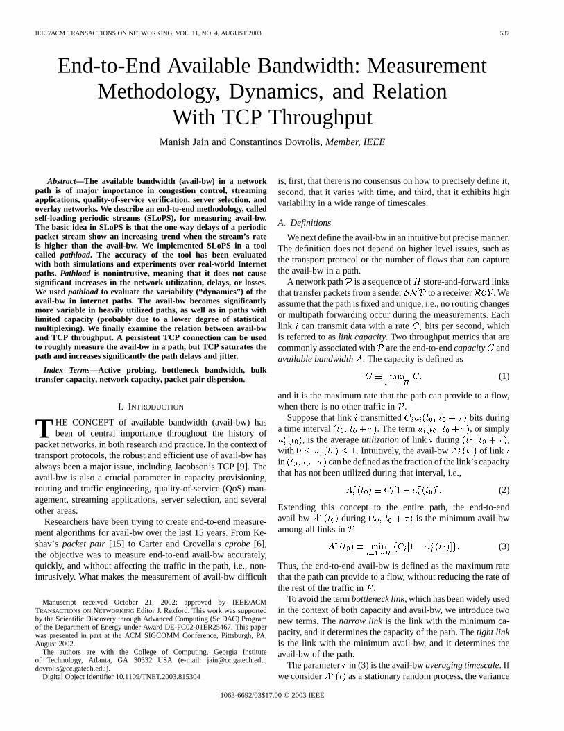
To gain some insight into this issue, Figs. 1–3 show the OWDvariations in three periodic streams that crossed a 12-hop pathfrom Univ-Oregon to Univ-Delaware. All three streams have

packets with s. The 5-min average avail-bwin the path during these measurements was about 74 Mb/s, ac-cording to the MRTG utilization graph of the tight link. In Fig. 1,the stream rate is Mb/s, i.e., higher than the long-termavail-bw. Notice that the OWDs between successive packetsare not strictly increasing, as one would expect from Proposi-tion 1, but overall, the stream OWDs have a clearly increasingtrend. This is shown both by the fact that most packets havea higher OWD than their predecessors, and because the OWDof the last packet is about 4 ms larger than the OWD of the

3A better way to initializeR is described in [12].

Fig. 1. OWD variations for a periodic stream whenR > A.

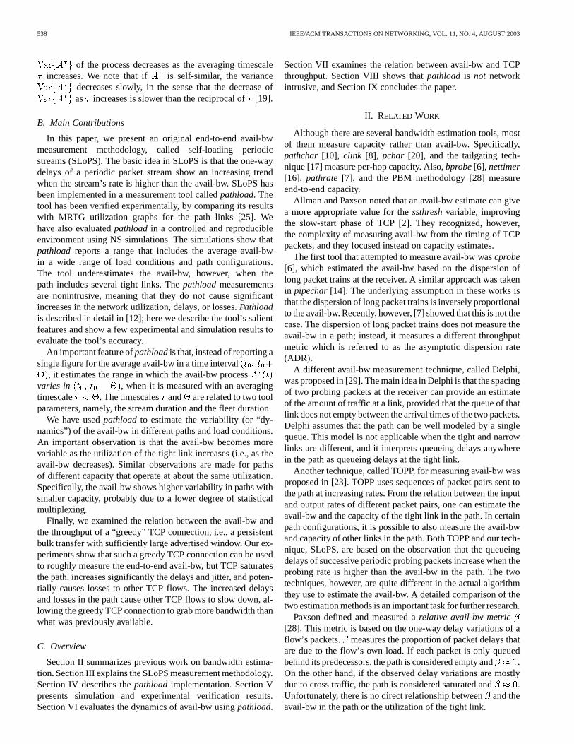
Fig. 2. OWD variations for a periodic stream whenR < A.

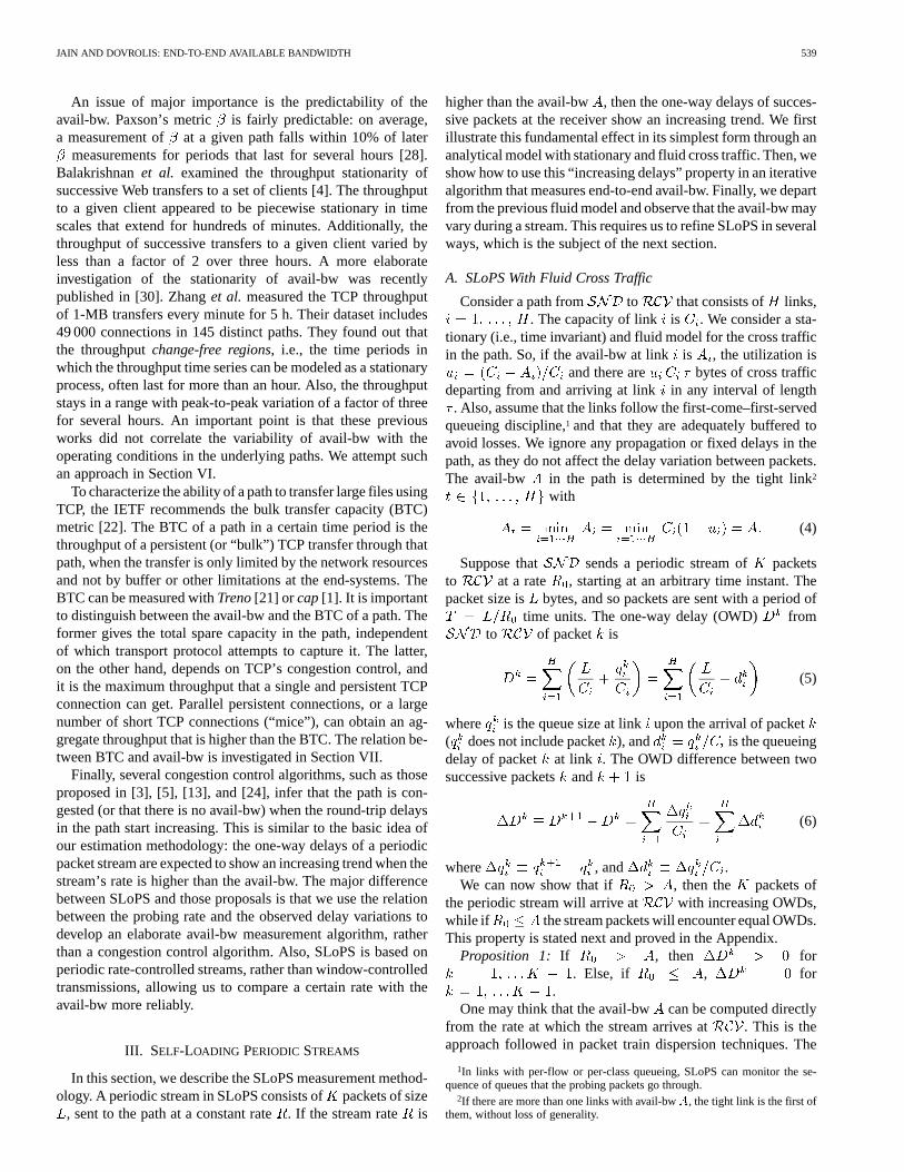
Fig. 3. OWD variations for a periodic stream whenR ./ A.

first packet. On the other hand, the stream of Fig. 2 has a rateMb/s, i.e., lower than the long-term avail-bw. Even

though there are short-term intervals in which we observe in-creasing OWDs, there is clearly not an increasing trend in thestream. The third stream, in Fig. 3, has a rate Mb/s. Thestream does not show an increasing trend in the first half, in-dicating that the avail-bw during that interval is higher than.The situation changes dramatically, however, after roughly the


60th packet. In that second half of the stream there is a clear in-creasing trend, showing that the avail-bw decreases to less than

.The previous example motivates two important refinements

in the SLoPS methodology. First, instead of analyzing the OWDvariations of a stream, expecting one of the two cases of Propo-sition 1 to be strictly true for every pair of packets, we shouldinstead watch for the presence of an overall increasing trendduring the entire stream. Second, we have to accept the possi-bility that the avail-bw may vary around rateduring a probingstream. In that case, there is no strict ordering betweenand

and, thus, a third possibility comes up, which we refer to asthe “grey region” (denoted as ). The next section gives aconcrete specification of these two refinements, as implementedin pathload.

IV. M EASUREMENTTOOL: PATHLOAD

We implemented SLoPS in a tool calledpathload. Pathload,together with its experimental verification, is described in detailin [12]. In this section, we provide a description of the tool’ssalient features.

Pathloadconsists of a process running at the senderand a process running at the receiver. The stream packetsuse UDP, while a TCP connection between the two end pointscontrols the measurements.

Clock and Timing Issues: timestamps each packetupon its transmission. So can measure the relative OWD

of packet that differs from the actual OWD by a certainoffset. This offset is due to the nonsynchronized clocks of theend-hosts. Since we are only interested in OWD differencesthough, a constant offset in the measured OWDs does not affectthe analysis. Clock skew can be a potential problem (and thereare algorithms to remove its effects) but not inpathload. Thereason is that each stream lasts for only a few milliseconds(Section IV), and so the skew during a stream is in the orderof nanoseconds, much less than the OWD variations due toqueueing.

Stream Parameters:A stream consists of packets of sizesent at a constant rate. is adjusted at runtime for each

stream, as described in Section IV. The packet interspacingisnormally set to , which is based on the minimum possibleperiod that the end hosts can achieve. The receiver measuresthe interspacing with which the packets left the sender, usingthe timestamps, to detect context switches and other ratedeviations [12].

Given and , the packet size is computed as ., however, has to be smaller than the path MTU (to

avoid fragmentation), and larger than a minimum possible sizeB. The reason for the constraint is to re-

duce the effect of layer-2 headers on the stream rate [26]. If, the interspacing is increased to .

The maximum rate thatpathloadcan generate, and thus themaximum avail-bw that it can measure, is .

The stream length is chosen based on two constraints. First,a stream should be relatively short, so that it does not causelarge queues and potential losses in the path routers. Second,

controls the stream duration , which is relatedto the averaging timescale (see Section VI-C). A larger(longer stream) increasesand, thus, reduces the variability inthe measured avail-bw. Inpathload, the default value for is100 packets.

Detecting an Increasing OWD Trend:Suppose that the(relative) OWDs of a particular stream are .As a preprocessing step, we partition these measurements into

groups of consecutive OWDs. Then, we computethe median OWD of each group.Pathload analyzes theset , which is more robust to outliers anderrors.

We use two complementary statistics to check if a streamshows an increasing trend. The pairwise comparison test (PCT)metric of a stream is

(8)

where is one if holds, and zero otherwise. PCT mea-sures the fraction of consecutive OWD pairs that are increasing,and so . If the OWDs are independent, the ex-pected value of is 0.5. If there is a strong increasing trend,

approaches one.The pairwise difference test (PDT) metric of a stream is

(9)

PDT quantifies how strong is the start-to-end OWD variation,relative to the OWD absolute variations during the stream. Notethat . If the OWDs are independent, the ex-pected value of is zero. If there is a strong increasingtrend, approaches one.

There are cases in which one of the two metrics is better thanthe other in detecting an increasing trend [12]. Consequently,if either the PCT or PDT metrics shows an increasing trend,pathloadcharacterizes the stream astype I, i.e., increasing. Oth-erwise, the stream is considered to betype N, i.e., nonincreasing.In the current release ofpathload, the PCT metric shows an in-creasing trend if , while the PDT shows increasingtrend if . The effect of the PCT and PDT thresholds(0.55 and 0.4, respectively) on thepathloadaccuracy is shownin the next section.

Fleets of Streams: Pathloaddoes not determine whetherbased on a single stream. Instead, it sends afleet of

streams, so that it samples whether successivetimes. All streams in a fleet have the same rate. Each streamis sent only when the previous stream has been acknowledged,to avoid a backlog of streams in the path. So, there is alwaysan idle interval between streams, which is larger than theround-trip time (RTT) of the path. The duration of a fleetis . Given and ,determines the fleet duration, which is related to thepathloadmeasurement latency. The default value foris 12 streams.The effect of is discussed in Section VI-D.


The averagepathloadrate during a fleet of rate is

In order to limit the averagepathloadrate to less than 10% of, the current version ofpathloadsets the interstream latency

to .If a stream encounters excessive losses (10%), or if more

than a number of streams within a fleet encounter moderatelosses ( 3%), the entire fleet is aborted and the rate of the nextfleet is decreased. For more details, see [12].

Grey Region: If a large fraction of the streams in afleet are of type I, the entire fleet shows an increasing trend andwe infer that the fleet rate is larger than the avail-bw ( ).Similarly, if a fraction of the streams are of type N, thefleet does not show an increasing trend and we infer that thefleet rate is smaller than the avail-bw ( ). It can happen,though, that less than streams are of type I, and alsothat less than streams are of type N. In that case, somestreams “sampled” the path when the avail-bw was less than

(type I), and some others when it was more than(typeN). We say, then, that the fleet rate is in the grey regionof the avail-bw, and write . The interpretation that wegive to the grey region is that when , the avail-bwprocess during that fleet varied above and below rate

, causing some streams to be of type I and some others tobe of type N. The averaging timescalehere is related to thestream duration . We discuss the effect of on thepathloadoutcome in the next section.

Rate Adjustment Algorithm:After a fleet of rate isover, pathloaddetermines whether , ,or . The iterative algorithm that determines the rate

of the next fleet is quite similar to the binary-searchapproach of (7). However, there are two important differences.

First, together with the upper and lower bounds for theavail-bw and , pathloadalso maintains upper andlower bounds for the grey region, namely and .When , one of these bounds is updated dependingon whether (update ), or

(update ). If a grey region has notbeen detected up to that point, the next rate is chosen,as in (7), halfway between and . If a grey regionhas been detected, is set halfway betweenand when , or halfway betweenand when . The complete rate adjustmentalgorithm, including the initialization steps, is given in [12]. Itis important to note that this binary-search approach succeedsin converging to the avail-bw, as long as the avail-bw variationrange is strictly included in the range. Theexperimental and simulation results of the next section showthat this is the case generally, with the exception of paths thatinclude several tight links.

The second difference is thatpathloadterminates not onlywhen the avail-bw has been estimated within a certain resolution

(i.e., ), but also whenand , i.e., when both avail-bw boundaries arewithin from the corresponding grey-region boundaries. Theparameter is referred to as grey-region resolution.

Fig. 4. Simulation topology.

The tool eventually reports the range .Measurement Latency:Sincepathloadis based on an iter-

ative algorithm, it is hard to predict how long a measurementwill take. For the default tool parameters, and for a path with

Mb/s and ms, the tool needs less than 15 sto produce a final estimate. The measurement latency increasesas the absolute magnitude of the avail-bw and/or the width ofthe grey region increases, and it also depends on the resolutionparameters and .

V. VERIFICATION

The objective of this section is to evaluate the accuracy ofpathloadwith both NS simulations and experiments over realInternet paths.

A. Simulation Results

The following simulations evaluate the accuracy ofpathloadin a controlled and reproducible environment under variousload conditions and path configurations. Specifically, weimplemented thepathloadsender ( ) and receiver ( )in application-layer NS modules. The functionality of thesemodules is identical as in the originalpathload, with theexception of some features that are not required in a simulator(such as the detection of context switches).

In the following, we simulate the -hop topology of Fig. 4.The pathloadpackets enter the path in hop 1 and exit at hop

. The hop in the middle of the path is the tight link, and ithas capacity , avail-bw , and utilization . We refer tothe rest of the links asnontight, and consider the case wherethey all have the same capacity , avail-bw , and utiliza-tion . Cross-traffic is generated at each link from ten randomsources that, unless specified otherwise, generate Pareto interar-rivals with . The cross-traffic packet sizes are distributedas follows: 40% are 40 B, 50% are 550 B, and 10% are 1500 B.The end-to-end propagation delay in the path is 50 ms, and thelinks are sufficiently buffered to avoid packet losses. Anotherimportant factor is the relative magnitude of the avail-bw in thenontight links and in the tight link . To quantify this, wedefine thepath tightness factoras

(10)

Unless specified otherwise, the default parameters in the fol-lowing simulations are hops, Mb/s, ,

%, , while the PCT threshold is 0.55 andthe PDT threshold is 0.4.

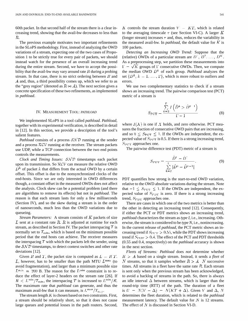
Fig. 5 examines the accuracy ofpathloadin four tight linkutilization values, ranging from light load ( %) to heavy


Fig. 5. Simulation results for different traffic types and tight link loads.

load ( %). We also consider two cross-traffic models: ex-ponential interarrivals and Pareto interarrivals with infinite vari-ance ( ). For each utilization and traffic model, we runpathload50 times to measure the avail-bw in the path. Aftereach run, the tool reports a range in which theavail-bw varies. Thepathloadrange that we show in Fig. 5 re-sults from averaging the 50 lower bounds and the 50 upperbounds . The coefficient of variation for the 50 samples of

and in the following simulations was typically be-tween 0.10 and 0.30.

The main observation in Fig. 5 is that pathload produces arange that includes the average avail-bw in the path, in bothlight and heavy load conditions at the tight link. This is true withboth the smooth interarrivals of Poisson traffic, and with the in-finite-variance Pareto model. For instance, when the avail-bwis 4 Mb/s, the averagepathloadrange in the case of Pareto in-terarrivals is from 2.4 to 5.6 Mb/s. It is also important to notethat the center of thepathloadrange is relatively close to the av-erage avail-bw. In Fig. 5, the maximum deviation between theaverage avail-bw and the center of thepathloadrange is whenthe former is 1 Mb/s and the latter is 1.5 Mb/s.

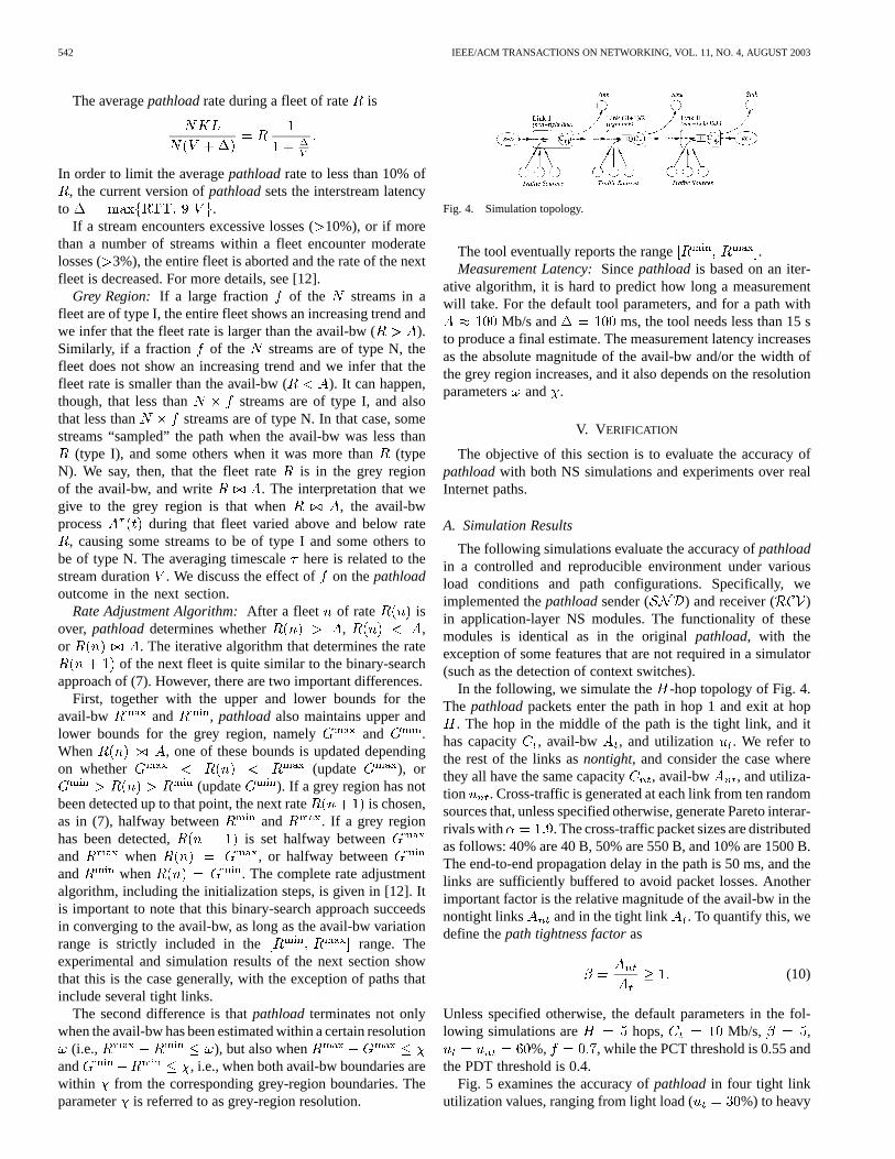
The next issue is whether the accuracy ofpathloaddependson the number and load of the nontight links. Fig. 6 shows, asin the previous paragraph, 50-sample averagepathloadrangesfor four different utilization points at the nontight links,and for two different path lengths . Since Mb/sand %, the end-to-end avail-bw in these simulations is4 Mb/s. The path tightness factor is , and so the avail-bwin the nontight links is Mb/s. So, even when there issignificant load and queueing at the nontight links (which is thecase when %), the end-to-end avail-bw is quite lowerthan the avail-bw in the nontight links.

The main observation in Fig. 6 is thatpathloadestimates arange that includes the actual avail-bw in all cases, indepen-dent of the number of nontight links or of their load. Also,the center of thepathloadrange is within 10% of the averageavail-bw . So, when the end-to-end avail-bw is mostly lim-ited by a single link,pathloadis able to estimate accurately theavail-bw in a multihop path even when there are several otherqueueing points. The nontight links introduce noise in the OWD

Fig. 6. Simulation results for different nontight link loads.

Fig. 7. Simulation results for different path tightness factors�.

of pathloadstreams, but they do not affect the OWD trend thatis formed when the stream goes through the tight link.

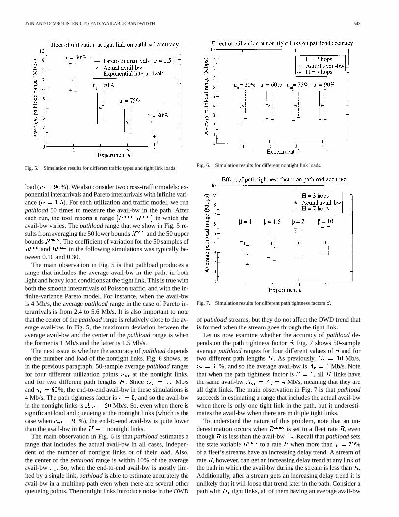
Let us now examine whether the accuracy ofpathloadde-pends on the path tightness factor. Fig. 7 shows 50-sampleaveragepathloadranges for four different values of and fortwo different path lengths . As previously, Mb/s,

%, and so the average avail-bw is Mb/s. Notethat when the path tightness factor is , all links havethe same avail-bw Mb/s, meaning that they areall tight links. The main observation in Fig. 7 is thatpathloadsucceeds in estimating a range that includes the actual avail-bwwhen there is only one tight link in the path, but it underesti-mates the avail-bw when there are multiple tight links.

To understand the nature of this problem, note that an un-derestimation occurs when is set to a fleet rate , eventhough is less than the avail-bw . Recall thatpathloadsetsthe state variable to a rate when more than %of a fleet’s streams have an increasing delay trend. A stream ofrate , however, can get an increasing delay trend at any link ofthe path in which the avail-bw during the stream is less than.Additionally, after a stream gets an increasing delay trend it isunlikely that it will loose that trend later in the path. Consider apath with tight links, all of them having an average avail-bw


Fig. 8. Simulation results for different values of fractionf .

. Suppose that is the probability that a stream of ratewill get an increasing delay trend at a tight link, even though

. Assuming that the avail-bw variations at different linksare independent, the probability that the stream will have an in-creasing delay trend after tight links is , whichincreases very quickly with . This explains why the under-estimation error in Fig. 7 appears whenis close to one (i.e.,

), and why it is more significant with rather thanwith three hops.

Finally, we examine the effect of and of the PCT/PDTthresholds on thepathloadresults.

Fig. 8 shows the effect of on thepathloadestimates. Thereportedpathloadrange, here, is a result of a singlepathloadrun. In these simulations, Mb/s, %,and so the average avail-bw in the path is Mb/s. Notethatas increases, the width of the grey region, and hence therange of the estimated avail-bw, increases as well. The reason isthat, for a given and , a higher means that a larger fractionof streams must be of type I when (or of type N when

) in order to correctly characterize the entire fleet asincreasing (or nonincreasing when ).

Fig. 9 shows the effect of the PDT threshold on thepathloadestimates. The simulation parameters are as in Fig. 8, but herewe use only the PDT metric to detect increasing delay trend.Note thatpathloadunderestimates the avail-bw when the PDTthreshold is too small ( 0), and it overestimates the avail-bwwhen the PDT threshold is too large (1). To understand why,recall that a stream is characterized as type I if is largerthan the PDT threshold. A small PDT threshold means that astream can be marked as type I even if . Similarly, witha large PDT threshold, a stream can be marked as type N evenif . The PCT threshold has a similar effect on the accu-racy ofpathload; we do not include those results due to spaceconstraints.

B. Experimental Results

We have also verifiedpathloadexperimentally, comparing itsoutput with the avail-bw shown in the MRTG [25] graph of thepath’s tight link. Even though this verification methodology isnot very accurate, it was the only way in which we could eval-uatepathload in real and wide-area Internet paths. For addi-

Fig. 9. Simulation results for different values of the PDT threshold.

Fig. 10. Verification experiment.

tional experimental results, and information about the use ofMRTG in the verification ofpathload, see [12].

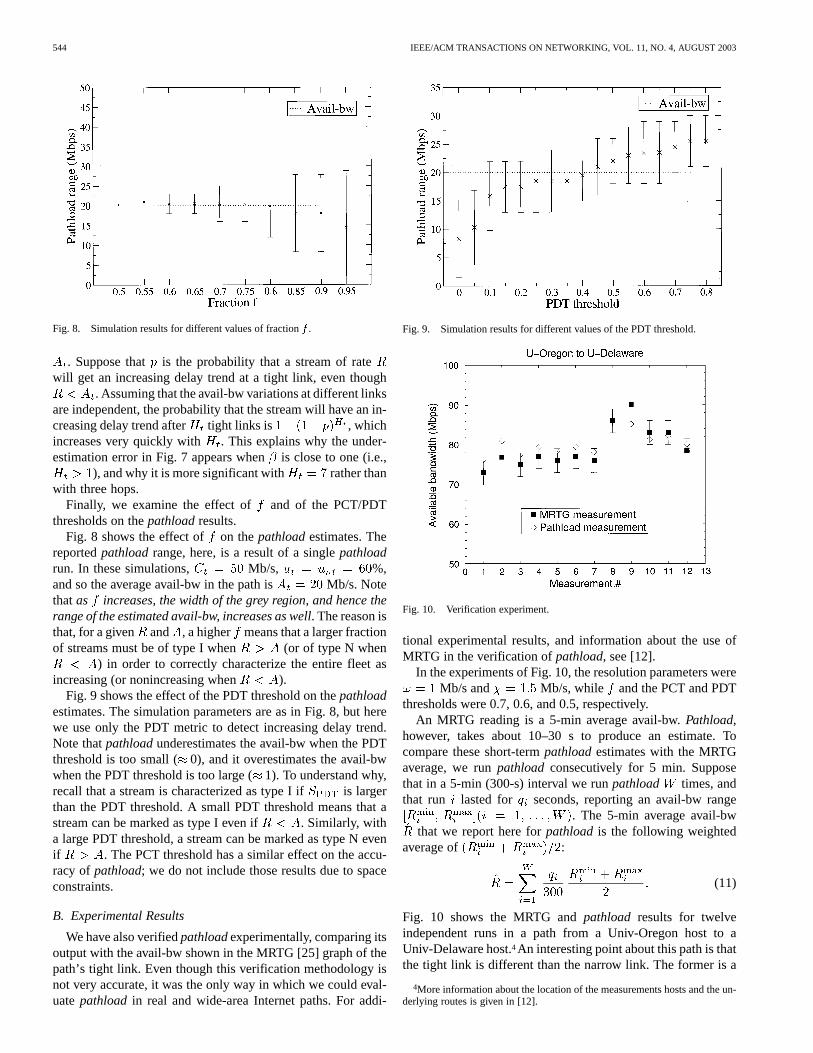
In the experiments of Fig. 10, the resolution parameters wereMb/s and Mb/s, while and the PCT and PDT

thresholds were 0.7, 0.6, and 0.5, respectively.An MRTG reading is a 5-min average avail-bw.Pathload,

however, takes about 10–30 s to produce an estimate. Tocompare these short-termpathloadestimates with the MRTGaverage, we runpathload consecutively for 5 min. Supposethat in a 5-min (300-s) interval we runpathload times, andthat run lasted for seconds, reporting an avail-bw range

. The 5-min average avail-bwthat we report here forpathloadis the following weighted

average of :

(11)

Fig. 10 shows the MRTG andpathload results for twelveindependent runs in a path from a Univ-Oregon host to aUniv-Delaware host.4An interesting point about this path is thatthe tight link is different than the narrow link. The former is a

4More information about the location of the measurements hosts and the un-derlying routes is given in [12].


155-Mb/s POS OC-3 link, while the latter is a 100-Mb/s FastEthernet interface. The MRTG readings are given as 6-Mb/sranges, due to the limited resolution of the graphs. Note thatthe pathloadestimate falls within the MRTG range in ten outof the twelve runs, while the deviations are marginal in the twoother runs.

VI. A VAILABLE BANDWIDTH DYNAMICS

In this section, we usepathloadto evaluate the variability ofthe avail-bw in different timescales and operating conditions.Given that our experiments are limited to a few paths, we donot attempt to make quantitative statements about the avail-bwvariability in the Internet. Instead, our objective is to show therelative effect of certain operational factors on the variability ofthe avail-bw.

In the following experiments, Mb/s and Mb/s.Note that because , pathloadterminates due to the con-straint only if there is no grey region; otherwise, it exits due tothe constraint. So, the final range thatpathloadreports is either at most 1 Mb/s () wide, indicating that thereis no grey region, or it overestimates the width of the grey re-gion by at most 2. Thus, is within 2 (or ) ofthe range in which the avail-bw varied during that pathload run.To compare the variability of the avail-bw across different op-erating conditions and paths, we define the following relativevariation metric:

(12)

In the following graphs, we plot the {5, 15, , 95} percentilesof based on 110pathloadruns for each experiment.

A. Variability and Load Conditions

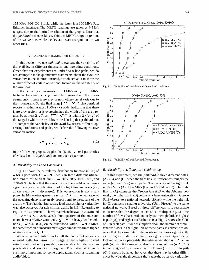
Fig. 11 shows the cumulative distribution function (CDF) offor a path with Mb/s in three different utiliza-

tion ranges of the tight link: 20%–30%, 40%–50%, and75%–85%. Notice that the variability of the avail-bw increasessignificantly as the utilization of the tight link increases (i.e.,as the avail-bw decreases). This observation is not a sur-prise. In Markovian queues, say, in , the variance ofthe queueing delay is inversely proportional to the square of theavail-bw. The fact that increasing load causes higher variabilitywas also observed for self-similar traffic in [19]. Returning toFig. 11, the 75 percentile shows that when the avail-bw is around

Mb/s ( 20%–30%), three quarters of the measure-ments have a relative variation . In heavy-load condi-tions ( 75%–85%) on the other hand, when –3 Mb/s,the same fraction of measurements give almost five times higherrelative variation ( ).

We observed a similar trend in all the paths that we exper-imented with. For users, this suggests that a lightly loadednetwork will not only provide more avail-bw, but also a morepredictable and smooth throughput. This latter attribute iseven more important for some applications, such as streamingaudio/video.

Fig. 11. Variability of avail-bw in different load conditions.

Fig. 12. Variability of avail-bw in different paths.

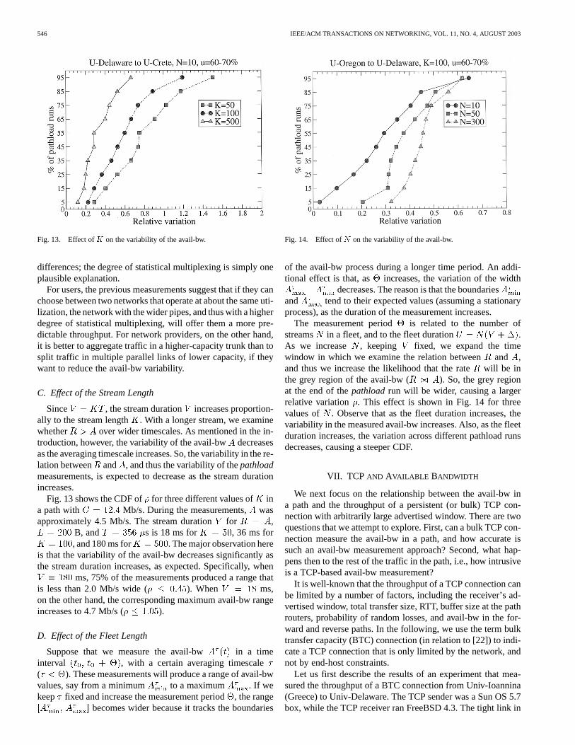
B. Variability and Statistical Multiplexing

In this experiment, we runpathloadin three different paths,(A), (B), and (C), when the tight link utilization was roughly thesame (around 65%) in all paths. The capacity of the tight linkis 155 Mb/s (A), 12.4 Mb/s (B), and 6.1 Mb/s (C). The tightlink in (A) connects the Oregon GigaPoP to the Abilene net-work, the tight link in (B) connects a large university in Greece(Univ-Crete) to a national network (GRnet), while the tight linkin (C) connects a smaller university (Univ-Pireaus) to the samenational network. Based on these differences, it is reasonableto assume that the degree of statistical multiplexing, i.e., thenumber of flows that simultaneously use the tight link, is highestin path (A), and higher in (B) than in (C). Fig. 12 shows the CDFof in each path. If our assumption about the number of simul-taneous flows in the tight link of these paths is correct, we ob-serve that the variability of the avail-bw decreases significantlyas the degree of statistical multiplexing increases. Specifically,looking at the 75 percentile, the relative variation is inpath (A), and it increases by almost a factor of two ( )in path (B), and by almost a factor of three ( ) in path(C). It should be noted, however, that there may be other differ-ences between the three paths that cause the observed variability


Fig. 13. Effect ofK on the variability of the avail-bw.

differences; the degree of statistical multiplexing is simply oneplausible explanation.

For users, the previous measurements suggest that if they canchoose between two networks that operate at about the same uti-lization, the network with the wider pipes, and thus with a higherdegree of statistical multiplexing, will offer them a more pre-dictable throughput. For network providers, on the other hand,it is better to aggregate traffic in a higher-capacity trunk than tosplit traffic in multiple parallel links of lower capacity, if theywant to reduce the avail-bw variability.

C. Effect of the Stream Length

Since , the stream duration increases proportion-ally to the stream length . With a longer stream, we examinewhether over wider timescales. As mentioned in the in-troduction, however, the variability of the avail-bwdecreasesas the averaging timescale increases. So, the variability in the re-lation between and , and thus the variability of thepathloadmeasurements, is expected to decrease as the stream durationincreases.

Fig. 13 shows the CDF of for three different values of ina path with Mb/s. During the measurements,wasapproximately 4.5 Mb/s. The stream durationfor ,

B, and s is 18 ms for , 36 ms for, and 180 ms for . The major observation here

is that the variability of the avail-bw decreases significantly asthe stream duration increases, as expected. Specifically, when

ms, 75% of the measurements produced a range thatis less than 2.0 Mb/s wide ( ). When ms,on the other hand, the corresponding maximum avail-bw rangeincreases to 4.7 Mb/s ( ).

D. Effect of the Fleet Length

Suppose that we measure the avail-bw in a timeinterval , with a certain averaging timescale( ). These measurements will produce a range of avail-bwvalues, say from a minimum to a maximum . If wekeep fixed and increase the measurement period, the range

becomes wider because it tracks the boundaries

Fig. 14. Effect ofN on the variability of the avail-bw.

of the avail-bw process during a longer time period. An addi-tional effect is that, as increases, the variation of the width

decreases. The reason is that the boundariesand tend to their expected values (assuming a stationaryprocess), as the duration of the measurement increases.

The measurement period is related to the number ofstreams in a fleet, and to the fleet duration .As we increase , keeping fixed, we expand the timewindow in which we examine the relation betweenand ,and thus we increase the likelihood that the ratewill be inthe grey region of the avail-bw ( ). So, the grey regionat the end of thepathloadrun will be wider, causing a largerrelative variation . This effect is shown in Fig. 14 for threevalues of . Observe that as the fleet duration increases, thevariability in the measured avail-bw increases. Also, as the fleetduration increases, the variation across different pathload runsdecreases, causing a steeper CDF.

VII. TCP AND AVAILABLE BANDWIDTH

We next focus on the relationship between the avail-bw ina path and the throughput of a persistent (or bulk) TCP con-nection with arbitrarily large advertised window. There are twoquestions that we attempt to explore. First, can a bulk TCP con-nection measure the avail-bw in a path, and how accurate issuch an avail-bw measurement approach? Second, what hap-pens then to the rest of the traffic in the path, i.e., how intrusiveis a TCP-based avail-bw measurement?

It is well-known that the throughput of a TCP connection canbe limited by a number of factors, including the receiver’s ad-vertised window, total transfer size, RTT, buffer size at the pathrouters, probability of random losses, and avail-bw in the for-ward and reverse paths. In the following, we use the term bulktransfer capacity (BTC) connection (in relation to [22]) to indi-cate a TCP connection that is only limited by the network, andnot by end-host constraints.

Let us first describe the results of an experiment that mea-sured the throughput of a BTC connection from Univ-Ioannina(Greece) to Univ-Delaware. The TCP sender was a Sun OS 5.7box, while the TCP receiver ran FreeBSD 4.3. The tight link in


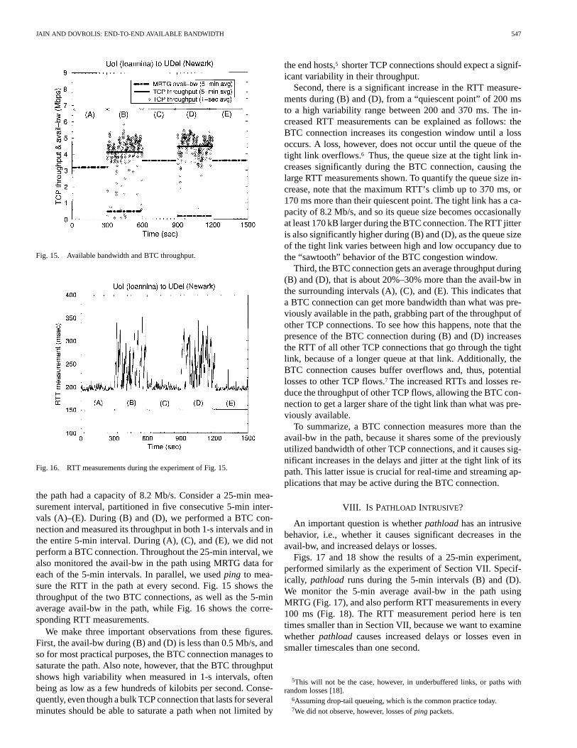
Fig. 15. Available bandwidth and BTC throughput.

Fig. 16. RTT measurements during the experiment of Fig. 15.

the path had a capacity of 8.2 Mb/s. Consider a 25-min mea-surement interval, partitioned in five consecutive 5-min inter-vals (A)–(E). During (B) and (D), we performed a BTC con-nection and measured its throughput in both 1-s intervals and inthe entire 5-min interval. During (A), (C), and (E), we did notperform a BTC connection. Throughout the 25-min interval, wealso monitored the avail-bw in the path using MRTG data foreach of the 5-min intervals. In parallel, we usedping to mea-sure the RTT in the path at every second. Fig. 15 shows thethroughput of the two BTC connections, as well as the 5-minaverage avail-bw in the path, while Fig. 16 shows the corre-sponding RTT measurements.

We make three important observations from these figures.First, the avail-bw during (B) and (D) is less than 0.5 Mb/s, andso for most practical purposes, the BTC connection manages tosaturate the path. Also note, however, that the BTC throughputshows high variability when measured in 1-s intervals, oftenbeing as low as a few hundreds of kilobits per second. Conse-quently, even though a bulk TCP connection that lasts for severalminutes should be able to saturate a path when not limited by

the end hosts,5 shorter TCP connections should expect a signif-icant variability in their throughput.

Second, there is a significant increase in the RTT measure-ments during (B) and (D), from a “quiescent point” of 200 msto a high variability range between 200 and 370 ms. The in-creased RTT measurements can be explained as follows: theBTC connection increases its congestion window until a lossoccurs. A loss, however, does not occur until the queue of thetight link overflows.6 Thus, the queue size at the tight link in-creases significantly during the BTC connection, causing thelarge RTT measurements shown. To quantify the queue size in-crease, note that the maximum RTT’s climb up to 370 ms, or170 ms more than their quiescent point. The tight link has a ca-pacity of 8.2 Mb/s, and so its queue size becomes occasionallyat least 170 kB larger during the BTC connection. The RTT jitteris also significantly higher during (B) and (D), as the queue sizeof the tight link varies between high and low occupancy due tothe “sawtooth” behavior of the BTC congestion window.

Third, the BTC connection gets an average throughput during(B) and (D), that is about 20%–30% more than the avail-bw inthe surrounding intervals (A), (C), and (E). This indicates thata BTC connection can get more bandwidth than what was pre-viously available in the path, grabbing part of the throughput ofother TCP connections. To see how this happens, note that thepresence of the BTC connection during (B) and (D) increasesthe RTT of all other TCP connections that go through the tightlink, because of a longer queue at that link. Additionally, theBTC connection causes buffer overflows and, thus, potentiallosses to other TCP flows.7 The increased RTTs and losses re-duce the throughput of other TCP flows, allowing the BTC con-nection to get a larger share of the tight link than what was pre-viously available.

To summarize, a BTC connection measures more than theavail-bw in the path, because it shares some of the previouslyutilized bandwidth of other TCP connections, and it causes sig-nificant increases in the delays and jitter at the tight link of itspath. This latter issue is crucial for real-time and streaming ap-plications that may be active during the BTC connection.

VIII. I S PATHLOAD INTRUSIVE?

An important question is whetherpathloadhas an intrusivebehavior, i.e., whether it causes significant decreases in theavail-bw, and increased delays or losses.

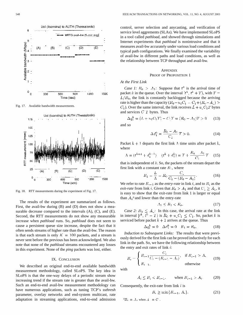
Figs. 17 and 18 show the results of a 25-min experiment,performed similarly as the experiment of Section VII. Specif-ically, pathload runs during the 5-min intervals (B) and (D).We monitor the 5-min average avail-bw in the path usingMRTG (Fig. 17), and also perform RTT measurements in every100 ms (Fig. 18). The RTT measurement period here is tentimes smaller than in Section VII, because we want to examinewhetherpathload causes increased delays or losses even insmaller timescales than one second.

5This will not be the case, however, in underbuffered links, or paths withrandom losses [18].

6Assuming drop-tail queueing, which is the common practice today.7We did not observe, however, losses ofping packets.


Fig. 17. Available bandwidth measurements.

Fig. 18. RTT measurements during the experiment of Fig. 17.

The results of the experiment are summarized as follows.First, the avail-bw during (B) and (D) does not show a mea-surable decrease compared to the intervals (A), (C), and (E).Second, the RTT measurements do not show any measurableincrease whenpathload runs. So,pathloaddoes not seem tocause a persistent queue size increase, despite the fact that itoften sends streams of higher rate than the avail-bw. The reasonis that each stream is only packets, and a stream isnever sent before the previous has been acknowledged. We alsonote that none of thepathloadstreams encountered any lossesin this experiment. None of theping packets was lost, either.

IX. CONCLUSION

We described an original end-to-end available bandwidthmeasurement methodology, called SLoPS. The key idea inSLoPS is that the one-way delays of a periodic stream showincreasing trend if the stream rate is greater than the avail-bw.Such an end-to-end avail-bw measurement methodology canhave numerous applications, such as tuning TCP’sssthreshparameter, overlay networks and end-system multicast, rateadaptation in streaming applications, end-to-end admission

control, server selection and anycasting, and verification ofservice level aggrements (SLAs). We have implemented SLoPSin a tool calledpathload, and showed through simulations andInternet experiments thatpathload is nonintrusive and that itmeasures avail-bw accurately under various load conditions andtypical path configurations. We finally examined the variabilityof avail-bw in different paths and load conditions, as well asthe relationship between TCP throughput and avail-bw.

APPENDIX

PROOF OFPROPOSITION1

At the First Link

Case 1: : Suppose that is the arrival time ofpacket in the queue. Over the interval , with

, the link is constantly backlogged because the arrivingrate is higher than the capacity (

). Over the same interval, the link receives bytesand services bytes. Thus

(13)

and so

(14)

Packet departs the first link time units after packet,where

(15)

that is independent of. So, the packets of the stream depart thefirst link with a constant rate , where

(16)

We refer to rate as theentry-ratein link , and to as theexit-ratefrom link . Given that and that , itis easy to show that the exit-rate from link 1 is larger or equalthan 8 and lower than the entry-rate

(17)

Case 2: : In this case, the arrival rate at the linkin interval is . So, packet isserviced before packet arrives at the queue. Thus

(18)

Induction to Subsequent Links:The results that were previ-ously derived for the first link can be proved inductively for eachlink in the path. So, we have the following relationship betweenthe entry and exit rates of link:

if

otherwise(19)

with

when (20)

Consequently, the exit-rate from linkis

(21)

8R = A whenA = C .


Also, the queueing delay difference between successive packetsat link is

if

otherwise.(22)

OWD Variations: If , we can apply (20) recursivelyfor to show that the stream will arrive atthe tight link with a rate . Thus, based on(22), , and so the OWD difference between successivepackets will be positive, .

On the other hand, if , then for everylink (from the definition of ). So, applying (21) recursivelyfrom the first link to the last, we see that for

. Thus, (22) shows that the delay difference in eachlink is , and so the OWD differences are .

ACKNOWLEDGMENT

The authors would like to thank the following colleaguesfor providing them with computer accounts at their sites:C. Douligeris (Univ-Pireaus), L. Georgiadis (AUTH), E.Markatos (Univ-Crete), D. Meyer (Univ-Oregon), M. Paterakis(Technical Univ-Crete), I. Stavrakakis (Univ-Athens), and L.Tassiulas (Univ-Ioannina). They would also like to thank theanonymous referees for their many constructive comments, andM. Seaver for her suggestions on the terminology.

REFERENCES

[1] M. Allman, “Measuring end-to-end bulk transfer capacity,” inProc.ACM SIGCOMM Internet Measurement Workshop, Nov. 2001, pp.139–143.

[2] M. Allman and V. Paxson, “On estimating end-to-end network pathproperties,” inProc. ACM SIGCOMM, Sept. 1999, pp. 263–274.

[3] A. A. Awadallah and C. Rai, “TCP-BFA: Buffer Fill Avoidance,”in Proc. IFIP High Performance Networking Conf., Sept. 1998, pp.575–594.

[4] H. Balakrishnan, S. Seshan, M. Stemm, and R. H. Katz, “Analyzing sta-bility in wide-area network performance,” inProc. ACM SIGMETRICS,June 1997, pp. 2–12.

[5] L. S. Brakmo, S. W. O’Malley, and L. L. Peterson, “TCP Vegas: Newtechniques for congestion detection and avoidance,” inProc. ACM SIG-COMM, Aug. 1994, pp. 24–35.

[6] R. L. Carter and M. E. Crovella, “Measuring bottleneck link speed inpacket-switched networks,”Perform. Eval., vol. 27, no. 28, pp. 297–318,1996.

[7] C. Dovrolis, P. Ramanathan, and D. Moore, “What do packet disper-sion techniques measure?,” inProc. IEEE INFOCOM, Apr. 2001, pp.905–914.

[8] A. B. Downey, “Using Pathchar to estimate Internet link characteristics,”in Proc. ACM SIGCOMM, Sept. 1999, pp. 222–223.

[9] V. Jacobson, “Congestion avoidance and control,” inProc. ACM SIG-COMM, Sept. 1988, pp. 314–329.

[10] , (1997, Apr.) Pathchar: A tool to infer characteristics of Internetpaths. [Online]. Available: ftp://ftp.ee.lbl.gov/pathchar/

[11] M. Jain and C. Dovrolis, “End-to-end available bandwidth: Measure-ment methodology, dynamics, and relation with TCP throughput,” inProc. ACM SIGCOMM, Aug. 2002, pp. 295–308.

[12] , “Pathload: A measurement tool for end-to-end available band-width,” in Proc. Passive and Active Measurements (PAM) Workshop,Mar. 2002, pp. 14–25.

[13] R. Jain, “A delay-based approach for congestion avoidance in inter-connected heterogeneous computer networks,”ACM Comput. Commun.Rev., vol. 19, no. 5, pp. 56–71, Oct. 1989.

[14] G. Jin, G. Yang, B. Crowley, and D. Agarwal, “Network Characteriza-tion Service (NCS),” inProc. 10th IEEE Symp. High Performance Dis-tributed Computing, Aug. 2001, pp. 289–299.

[15] S. Keshav, “A control-theoretic approach to flow control,” inProc. ACMSIGCOMM, Sept. 1991, pp. 3–15.

[16] K. Lai and M. Baker, “Measuring bandwidth,” inProc. IEEE IN-FOCOM, Apr. 1999, pp. 235–245.

[17] , “Measuring link bandwidths using a deterministic model of packetdelay,” inProc. ACM SIGCOMM, Sept. 2000, pp. 283–294.

[18] T. V. Lakshman and U. Madhow, “The performance of TCP/IP fornetworks with high bandwidth delay products and random losses,”IEEE/ACM Trans. Networking, vol. 5, pp. 336–350, June 1997.

[19] W. E. Leland, M. S. Taqqu, W. Willinger, and D. V. Wilson, “On theself-similar nature of ethernet traffic (Extended Version),”IEEE/ACMTrans. Networking, vol. 2, pp. 1–15, Feb. 1994.

[20] B. A. Mah. (1999, Feb.) Pchar: A tool for measuring Internet path char-acteristics. [Online]. Available: http://www.employees.org/~bmah/Soft-ware/pchar/

[21] M. Mathis. (1999, Feb.) TReno bulk transfer capacity. IETF, InternetDraft. [Online]. Available: http://www.advanced.org/IPPM/docs/draft-ietf-ippm-treno-btc-03.txt

[22] M. Mathis and M. Allman. (2001, July) A framework for defining em-pirical bulk transfer capacity metrics. IETF, RFC 3148. [Online]. Avail-able: http://www1.ietf.org/rfc/rfc3148.txt

[23] B. Melander, M. Bjorkman, and P. Gunningberg, “A new end-to-endprobing and analysis method for estimating bandwidth bottlenecks,” inProc. IEEE Globecom, 2000, pp. 415–420.

[24] D. Mitra and J. B. Seery, “Dynamic adaptive windows for high-speeddata networks: Theory and simulations,” inProc. ACM SIGCOMM,Aug. 1990, pp. 30–40.

[25] T. Oetiker. MRTG: Multi Router Traffic Grapher. Swiss Fed-eral Inst. Technology, Zurich. [Online]. Available: http://ee-staff.ethz.ch/~oetiker/webtools/mrtg/mrtg.html

[26] A. Pasztor and D. Veitch, “The packet size dependence of packet pairlike methods,” inProc. IEEE/IFIP Int. Workshop Quality of Service(IWQoS), 2002, pp. 204–213.

[27] V. Paxson, “On calibrating measurements of packet transit times,” inProc. ACM SIGMETRICS, June 1998, pp. 11–21.

[28] , “End-to-end Internet packet dynamics,”IEEE/ACM Trans. Net-working, vol. 7, pp. 277–292, June 1999.

[29] V. Ribeiro, M. Coates, R. Riedi, S. Sarvotham, B. Hendricks, and R.Baraniuk, “Multifractal cross-traffic estimation,” inProc. ITC SpecialistSeminar IP Traffic Measurement, Modeling, and Management, Sept.2000.

[30] Y. Zhang, N. Duffield, V. Paxson, and S. Shenker, “On the constancy ofInternet path properties,” inProc. ACM SIGCOMM Internet Measure-ment Workshop, Nov. 2001, pp. 197–211.

Manish Jain received the B.Eng. degree in computerengineering from the Shri Govindram Sekseria Insti-tute of Technology and Science (SGSITS), Indore,India, in 1999 and the M.S. degree in computer sci-ence from the University of Delaware, Newark, in2002. He is currently working toward the Ph.D. de-gree at the College of Computing, Georgia Instituteof Technology, Atlanta.

His research interests include bandwidth estima-tion methologies and applications, TCP in high band-width networks, and network applications and ser-

vices.

Constantinos Dovrolis (M’93) received thecomputer engineering degree from the TechnicalUniversity of Crete, Crete, Greece, in 1995, theM.S. degree from the University of Rochester,Rochester, NY, in 1996, and the Ph.D. degree fromthe University of Wisconsin–Madison in 2000.

He is currently an Assistant Professor withthe College of Computing, Georgia Institute ofTechnology, Atlanta. His research interests includemethodologies and applications of network mea-surements, bandwidth estimation algorithms and

tools, service differentiation, and router architectures.

end-to-end available bandwidth: measurement methodology ...cs622/papers/p537-jain.pdf · end-to-end...

Documents