electrical load forecasting. modeling and model...

Butterworth–Heinemann is an imprint of Elsevier30 Corporate Drive, Suite 400, Burlington, MA 01803, USAThe Boulevard, Langford Lane, Kidlington, Oxford, OX5 1GB, UK

Copyright © 2010 Elsevier Inc. All rights reserved.

No part of this publication may be reproduced or transmitted in any form or by any means, electronic or mechanical,including photocopying, recording, or any information storage and retrieval system, without permission in writing from thePublisher. Details on how to seek permission, further information about the Publisher’s permissions policies, and ourarrangements with organizations such as the Copyright Clearance Center and the Copyright Licensing Agency can befound at our website: www.elsevier.com/permissions.

This book and the individual contributions contained in it are protected under copyright by the Publisher (other thanas may be noted herein).

NoticesKnowledge and best practice in this field are constantly changing. As new research and experience broaden ourunderstanding, changes in research methods, professional practices, or medical treatment may become necessary.

Practitioners and researchers must always rely on their own experience and knowledge in evaluating and using anyinformation, methods, compounds, or experiments described herein. In using such information or methods they should bemindful of their own safety and the safety of others, including parties for whom they have a professional responsibility.

To the fullest extent of the law, neither the Publisher, nor the authors, contributors, or editors, assume any liability for anyinjury and/or damage to persons or property as a matter of products liability, negligence or otherwise, or from any use oroperation of any methods, products, instructions, or ideas contained in the material herein.

Library of Congress Cataloging-in-Publication DataSoliman, S.A.Electrical load forecasting : modeling and model construction / Soliman Abdel-hady Soliman (S.A. Soliman),Ahmad M. Al-Kandari.p. cm.

Includes bibliographical references and index.ISBN 978-0-12-381543-9 (alk. paper)

1. Electric power-plants–Load–Forecasting–Mathematics. 2. Electric power systems–Mathematical models.3. Electric power consumption–Forecasting–Mathematics. I. Al-Kandari, Ahmad M. II. Title.TK1005.S64 2010333.793'213015195–dc22 2009048799

British Library Cataloguing-in-Publication DataA catalogue record for this book is available from the British Library.

For information on all Butterworth–Heinemann publicationsvisit our Web site at www.elsevierdirect.com

Typeset by: diacriTech, India

Printed in the United States of America10 11 12 13 14 10 9 8 7 6 5 4 3 2 1

To my parents, I was in need of them during my operationTo my wife, Laila, with love and respect

To my kids, Rasha, Shady, Samia, Hadeer,and Ahmad, I love you all

To everyone who has the same liver problem,please do not lose hope in God

(S. A. Soliman)

To my parents, who raised meTo my wife, Noureyah, with great love and respect

To my sons, Eng.Bader and Eng.Khalied,for their encouragement

To my beloved family and friends(A. M. Al-Kandari)

Acknowledgments

In the market and the community of electric power system engineers, there is a short-age of books focusing on short-term electric load forecasting. Many papers have beenpublished in the literature, but no book is available that contains all these publica-tions. The idea of writing this book came to my mind two or three years ago, butthe time was too limited to write such a big book. In the spring of 2009, I was diag-nosed with liver cancer, and I have had to treat it locally through chemical therapyuntil a suitable donor is available and I can have a liver transplant. The presidentof Misr University for Science and Technology, Professor Mohammad Rafat, andmy brothers, Professor Mostafa Kamel, vice president for academic affairs, and Pro-fessor Kamal Al-Bedawy, dean of engineering, asked me to stay at home to eliminatephysical stress. As such, I had a lot of time to write such a book, especially becausethere are many publications in the area of short-term load forecasting. Indeed, myappreciation goes to them and chancellor of Misr University, Mr. Khalied Al-Tokhay.

My appreciation goes to my wife, Laila, who did not sleep, sitting beside me dayand night while I underwent therapy. My appreciation also goes to my kids Rasha,Shady, Samia, Hadeer, and Ahmad, who raced to be the first donor for their dad.

My appreciation goes to my brothers-in-law, Eng. Ahmad Nabil Mousa, ProfessorMahmoud Rashad, and Dr. Samy Mousa, who had a hard time because of my illness;he never left me alone even though he was out of the city of Cairo. Furthermore, myappreciation goes also to my sons-in-law, Ahmad Abdel-Azim and MohammadAbdel-Azim.

My deep appreciation goes to Dr. Helal Al-Hamadi of Kuwait University, who wasthe coauthor with me for some materials we used in this book.

Many thanks also go to my friends and colleagues among the faculty of theengineering department at Misr University for Science and Technology. To them,I say, “You did something unbelievable.” In addition, many thanks to my friendsand colleagues among the faculty of the engineering department at Ain ShamsUniversity for their moral support. Special thanks go to my good friends ProfessorMahmoud Abdel-Hamid and Professor Ibrahim Helal, who forgot the misunderstand-ing between us and came to visit me at home on the same day he heard that I was sickand took me to his friend, Professor Mohammad Alwahash, who is a liver transplantexpert. Professor M. E. El-Hawary, of Dalhousie University, Nova Scotia Canada, myspecial friend, I miss you MO; I did everything that makes you happy in Egypt andCanada.

My deep appreciation goes to the team of liver transplantation and intensive careunits at the liver and kidney hospital of Al-Madi Military Medical Complex; Profes-sor Kareem Bodjema, the French excellent expert in liver transplantation; Professor

Magdy Amin, the man with whom I felt secure when he visited me in my room withhis colleagues, who answered my calls any time during the day or night, and whosupported me and my family morally; Professor Salah Aiaad, the man, in my firstmeeting with him, whom I felt I knew for a long time; Professor Ali Albadry; Profes-sor Mahmoud Negm, who has a beautiful smile; Professor Ehab Sabry, the man whocan easily read what’s in my eyes; and Dr. Mohammad Hesaan, who reminds me ofwhen I was in my forties—everything should go ideally for him.

Last, but not least, my deep appreciation and respect go to General Samir Hamam,the manager of Al-Madi Military Medical Complex, for helping to make everythinggo smoothly. To all, I say you did a good job in every position at the hospital. MayGod keep you all healthy and wealthy and remember these good things you did forme to the day after.

S.A. Soliman

It is a privilege to be a coauthor with as great a professor as Professor SolimanAbdel-hady Soliman. I learned a lot from him. I thank him for giving me the oppor-tunity to coauthor this book, which will cover a needed area in load forecasting. I dothank Professor M.E. El-Hawary for teaching me and guiding me in the scope of thematerial of this book. Also, my appreciation goes to Professor Yacoub Al-Refae,general director of The Public Authority for Applied Education and Training inKuwait, for his encouragements and notes.

A.M. Al-Kandari

The authors of this book would like to acknowledge the effort done by Ms. SarahBinns for reviewing this book many times and we appreciate her time. To her wesay, you did a good job for us, you were sincere and honest in every stage of this book.

xiv Acknowledgments

Introduction

Economic development, throughout the world, depends directly on the availability ofelectric energy, especially because most industries depend almost entirely on its use.The availability of a source of continuous, cheap, and reliable energy is of foremosteconomic importance.

Electrical load forecasting is an important tool used to ensure that the energy sup-plied by utilities meets the load plus the energy lost in the system. To this end, a staffof trained personnel is needed to carry out this specialized function. Load forecastingis always defined as basically the science or art of predicting the future load on agiven system, for a specified period of time ahead. These predictions may be justfor a fraction of an hour ahead for operation purposes, or as much as 20 years intothe future for planning purposes.

Load forecasting can be categorized into three subject areas—namely,

1. Long-range forecasting, which is used to predict loads as distant as 50 years ahead so thatexpansion planning can be facilitated.

2. Medium-range forecasting, which is used to predict weekly, monthly, and yearly peak loadsup to 10 years ahead so that efficient operational planning can be carried out.

3. Short-range forecasting, which is used to predict loads up to a week ahead so that daily run-ning and dispatching costs can be minimized.

In the preceding three categories, an accurate load model is required to mathema-tically represent the relationship between the load and influential variables such astime, weather, economic factors, etc. The precise relationship between the load andthese variables is usually determined by their role in the load model. After the math-ematical model is constructed, the model parameters are determined through the useof estimation techniques.

Extrapolating the mathematical relationship to the required lead time ahead andgiving the corresponding values of influential variables to be available or predictable,forecasts can be made. Because factors such as weather and economic indices areincreasingly difficult to predict accurately for longer lead times ahead, the greaterthe lead time, the less accurate the prediction is likely to be.

The final accuracy of any forecast thus depends on the load model employed, theaccuracy of predicted variables, and the parameters assigned by the relevant estima-tion technique. Because different methods of estimation will result in different valuesof estimated parameters, it follows that the resulting forecasts will differ in predictionaccuracy.

Over the past 50 years, the parameter estimation algorithms used in load forecastinghave been limited to those based on the least error squares minimization criterion, eventhough estimation theory indicates that algorithms based on the least absolute value cri-teria are viable alternatives. Furthermore, the artificial neural network (ANN) hadshowed success in estimating the load for the next hour. However, the ANN usedby a utility is not necessarily suitable for another utility and should be retrained tobe suitable for that utility.

It is well known that the electric load is a dynamic one and does not have a precisevalue from one hour to another. In this book, fuzzy systems theory is implemented toestimate the load model parameters, which are assumed to be fuzzy parameters havinga certain middle and spread. Different membership functions, for load parameters, areused—namely, triangular membership and trapezoidal membership functions. Theproblem of load forecasting in this book is restricted to short-term load forecastingand is formulated as a linear estimation problem in the parameters to be estimated.In this book, the parameters in the first part are assumed to be crisp parameters,whereas in the rest of the book these parameters are assumed to be fuzzy parameters.The objective is to minimize the spread of the available data points, taking into con-sideration the type of membership of the fuzzy parameters, subject to satisfying con-straints on each measurement point, to ensure that the original membership isincluded in the estimated membership.

Outline of the Book

In this book, different techniques used in the past two decades are implemented toestimate the load model parameters, including fuzzy parameters with certain middleand certain spread. The book contains nine chapters:

Chapter 1, “Mathematical Background and State of the Art.” This chapterintroduces mathematical background to help the reader understand the problems for-mulated in this book. In this chapter, the reader will study matrices and their applica-tions in estimation theory and see that the use of matrix notation simplifies complexmathematical expressions. The simplifying matrix notation may not reduce theamount of work required to solve mathematical equations, but it usually makes theequations much easier to handle and manipulate. This chapter explains the vectorsand the formulation of quadratic forms, and, as we shall see, that most objective func-tions to be minimized (least errors square criteria) are quadratic in nature. This chapteralso explains some optimization techniques and introduces the concept of a statespace model, which is commonly used in dynamic state estimation. The reader willalso review different techniques that, developed for the short term, give the state ofthe art of the various algorithms used during the past decades for short-term load fore-casting. A brief discussion for each algorithm is presented in this chapter. Advantagesand disadvantages of each algorithm are discussed. Reviewing the most recent pub-lications in the area of short-term load forecasting indicates that most of the availablealgorithms treat the parameters of the proposed load model as crisp parameters, whichis not the case in reality.

xvi Introduction

Chapter 2, “Static State Estimation.” This chapter presents the theory involvedin different approaches that use parameter estimation algorithms. In the first partof the chapter, the crisp parameter estimation algorithms are presented; they includethe least error squares (LES) algorithm and the least absolute value (LAV) algorithm.The second part of the chapter presents an introduction to fuzzy set theory and sys-tems, followed by a discussion of fuzzy linear regression algorithms. Different casesfor the fuzzy parameters are discussed in this part. The first case is for the fuzzy linearregression of the linear models having fuzzy parameters with nonfuzzy outputs, thesecond case is for the linear regression of fuzzy parameters with fuzzy output, andthe third case is for fuzzy parameters formulated with fuzzy output of left and righttype (LR-type).

Chapter 3, “Load Modeling for Short-Term Forecasting.” This chapter pro-poses different load models used in short-term load forecasting for 24 hours.

• Three models are proposed in this chapter—namely, models A, B, and C. Model A is a mul-tiple linear regression model of the temperature deviation, base load, and either wind-chillfactor for winter load or temperature humidity factor for summer load. The parameters ofload A are assumed to be crisp parameters in this chapter. The term crisp parametersmean clearly defined parameter values without ambiguity.

• Load model B is a harmonic decomposition model that expresses the load at any instant, t,as a harmonic series. In this model, the weekly cycle is accounted for through use of a dailyload model, the parameters of which are estimated seven times weekly. Again, the param-eters of this model are assumed to be crisp.

• Load model C is a hybrid load model that expresses the load as the sum of a time-varyingbase load and a weather-dependent component. This model is developed with the aim ofeliminating the disadvantages of the other two models by combining their modelingapproaches. After finding the parameter values, one uses them to determine the electricload from which these parameter values are extracted, and this value is called the estimatedload. Then the parameter values are used to predict the electric load for a randomly chosenday in the future, and it is called the predicted load for that chosen day.

Chapter 4, “Fuzzy Regression Systems and Fuzzy Linear Models.” The objec-tive of this chapter is to introduce principal concepts and mathematical notions offuzzy set theory, a theory of classes of objects with non sharp boundaries.

• We first review fuzzy sets as a generalization of classical crisp sets by extending the rangeof the membership function (or characteristic function) from [0, 1] to all real numbers in theinterval [0, 1].

• A number of notions of fuzzy sets, such as representation support, α-cuts, convexity, andfuzzy numbers, are then introduced. The resolution principle, which can be used to expanda fuzzy set in terms of its α-cuts, is discussed.

• This chapter introduces fuzzy mathematical programming and fuzzy multiple-objective deci-sion making. We first introduce the required knowledge of fuzzy set theory and fuzzy mathe-matics in this chapter.

• Fuzzy linear regression also is introduced in this chapter; the first part is to estimate thefuzzy regression coefficients when the set of measurements available is crisp, whereas inthe second part the fuzzy regression coefficients are estimated when the available set ofmeasurements is a fuzzy set with a certain middle and spread.

• Some simple examples for fuzzy linear regression are introduced in this chapter.

Introduction xvii

• The models proposed in Chapter 3 for crisp parameters are used in this chapter. Fuzzymodel A employs a multiple fuzzy linear regression model. The membership function forthe model parameters is developed, where triangular membership functions are assumedfor each parameter of the load model. Two constraints are imposed on each load measure-ment to ensure that the original membership is included in the estimated membership.

• Fuzzy model B, which is a harmonic model, also is proposed in this chapter. This modelinvolves fuzzy parameters having a certain median and certain spread.

• Finally, a hybrid fuzzy model C, which is the combination of the multiple linear regressionmodel A and harmonic model B, is presented in this chapter.

Chapter 5, “Dynamic State Estimation.” The objective of this chapter is to studythe dynamic state estimation problem and its applications to electric power systemanalysis, especially short-term load forecasting. Furthermore, the different approachesused to solve this dynamic estimation problem are also discussed in this chapter. Afterreading this chapter, the reader will be familiar with

The five fundamental components of an estimation problem:• The variables to be estimated.• The measurements or observations available.• The mathematical model describing how the measurements are related to the variable of

interest.• The mathematical model of the uncertainties present.• The performance evaluation criterion to judge which estimation algorithms are “best.”Formulation of the dynamic state estimation problem:• Kalman filtering algorithm as a recursive filter used to solve a problem.• Weighted least absolute value filter.• Different problems that face Kalman filtering and weighted least absolute value filtering

algorithms.

Chapter 6, “Load Forecasting Results Using Static State Estimation.” Theobjective of this chapter is as follows:

In Chapter 3, the models are derived on the basis that the load powers are crisp in nature; thedata available from a big company in Canada are used to forecast the load power in the crispcase.• In this chapter, the results obtained for the crisp load power data for the different load models

developed in Chapter 3 are shown.• A comparison is performed between the two static LES and LAV estimation techniques.• The parameters estimated are used to predict a load using both techniques, where we com-

pare between them for summer and winter.

Chapter 7, “Load Forecasting Results Using Fuzzy Systems.” Chapter 6 dis-cusses the short-term load-forecasting problem, and the LES and LAV parameter esti-mation algorithms are used to estimate the load model parameters. The error in theestimates is calculated for both techniques. The three models, proposed earlier inChapter 3, are used in that chapter to present the load in different days for differentseasons. In this chapter, the fuzzy load models developed in Chapter 5 are tested. Thefuzzy parameters of these models are estimated using the past history data for summerweekdays and weekend days as well as for winter weekdays and weekend days. Thenthese models are used to predict the fuzzy load power for 24 hours ahead, in both

xviii Introduction

summer and winter seasons. The results are given in the form of tables and figures forthe estimated and predicted loads.

Chapter 8, “Dynamic Electric Load Forecasting.” The main objectives of thischapter are as follows:

• A one-year long-term electric power load-forecasting problem is introduced as a first stepfor short-term load forecasting.

• A dynamic algorithm, the Kalman filtering algorithm, is suitable to forecast daily load pro-files with a lead-time from several weeks to a few years.

• The algorithm is based mainly on multiple simple linear regression models used to capturethe shape of the load over a certain period of time (one year) in a two-dimensional layout(24 hours � 52 weeks).

• The regression models are recursively used to project the 2D load shape for the next periodof time (next year). Load-demand annual growth is estimated and incorporated into theKalman filtering algorithm to improve the load-forecast accuracy obtained so far fromthe regression models.

Chapter 9, “Electric Load Modeling for Long-Term Forecasting.” The objec-tives of this chapter are as follows:

• This chapter provides a comparative study between two static estimation algorithms—namely, the least error squares (LES) and least absolute value (LAV) algorithms—for esti-mating the parameters of different load models for peak-load forecasting necessary for long-term power system planning.

• The proposed algorithms use the past history data for the load and the influence factors,such as gross domestic product (GDP), population, GDP per capita, system losses, loadfactor, etc.

• The problem turns out to be a linear estimation problem in the load parameters. Differentmodels are developed and discussed in the text.

Introduction xix

4 Fuzzy Regression Systems andFuzzy Linear Models

4.1 Objectives

The objectives of this chapter are

• Introducing principal concepts and mathematical notions of fuzzy set theory, a theory ofclasses of objects with nonsharp boundaries.

• Reviewing fuzzy sets as a generalization of classical crisp sets by extending the range of themembership function (or characteristic function) from [0, 1] to all real numbers in the inter-val [0, 1].

• Introducing a number of notions of fuzzy sets, such as representation support, α-cuts, con-vexity, and fuzzy numbers. We also discuss the resolution principle, which can be used toexpand a fuzzy set in terms of its α-cuts.

• Introducing fuzzy mathematical programming and fuzzy multiple-objective decision mak-ing. We first introduce the required knowledge behind fuzzy set theory and fuzzymathematics.

• Introducing fuzzy linear regression. The first part of this discussion describes how to esti-mate the fuzzy regression coefficients when the set of measurements available is crisp,whereas in the second part the fuzzy regression coefficients are estimated when the availableset of measurements is a fuzzy set with a certain middle and spread.

• Introducing some simple examples for fuzzy linear regression.

4.2 Fuzzy Fundamentals

Human beings make tools for their use and also want to control the tools as theydesire. A feedback concept is very important in being able to achieve control overthese tools. As modern plants with many inputs and outputs become more andmore complex, any description of a modern control system requires a large numberof equations. Since about 1960, modern control theory has been developed to copewith the increased complexity of modern plants. The most recent developmentsmay be said to be in the direction of optimal control of both deterministic and stochas-tic systems, as well as the adaptive and learning control of time-variant complex sys-tems. These developments have been accelerated through the use of digital computers.

Modern plants are designed for efficient analysis and production by human beings.We are now confronted with the need to control living cells, which are nonlinear,complex, time variant, and mysterious. They cannot be mastered easily throughclassical or control theory or even modern artificial intelligence (AI) employing a

Copyright © 2010 by Elsevier Inc. All rights reserved.DOI: 10.1016/B978-0-12-381543-9.00004-X

powerful digital computer. So we are faced with many problems, and our problemscan be seen in terms of decisions, management, and predictions. Solutions can beseen in terms of faster access to more information and of increased aid in analyzing,understanding, and utilizing the information that is not available. These two elements,a large amount of information coupled with a large amount of uncertainty, takentogether constitute the basis for many of our problems today: complexity. How dowe manage to cope with complexity as well as we do, and how could we manageto cope better? These are the reasons for introducing fuzzy notations becausethe fuzzy sets method is very useful for handling uncertainties and is essential forthe knowledge acquisition of human experts. First, we have to know what fuzzymeans? Fuzzy essentially means vague or imprecise information.

Everyday language provides one example of the way vagueness is used and pro-pagated; for example, consider driving a car or describing the weather or classifying aperson’s age. So using the term fuzzy is one way engineers describe the operation of asystem by means of fuzzy variables and terms. To solve any control problem, wemight have a variable. This variable is a crisp set in the conventional control method;that is, it has a definite value and a certain boundary in such a way it can be definedby two groups:

1. Members, or those that certainly belong in the set inside the boundary.2. Nonmembers, or those that certainly don’t belong.

But sometimes collections and categories have boundaries that seem vague,and the transition from member to nonmember appears gradual rather than abrupt.These collections and categories are what we call fuzzy sets. Thus, fuzzy sets area generalization of conventional set theory. Every fuzzy set can be represented bya membership function, and there is no unique membership. A function for anyfuzzy set, a membership function, exhibits a continuous curve changing from0 to 1 or vice versa, and this transition region represents a fuzzy boundary of the term.

For a computer language, we can define fuzzy logic as a method of easily repre-senting analog processes with continuous phenomena that are not easily brokendown into discrete segments, and the concepts involved are difficult to model some-times. In conclusion, we can use the term fuzzy when

1. One or more of the control variables are continuous.2. A mathematical model of the process does not exist, or it exists but is too difficult to encode.3. A mathematical model is too complex to be evaluated fast enough for real-time operation.4. A mathematical model involves too much memory on the designated chip architecture.5. An expert is available who can specify the rules underlying the system behavior and the

fuzzy sets that represent the characteristics of each variable.6. A system has uncertainties in either its inputs or definition.

On the other hand, for systems in which conventional control equations and meth-ods are already optimal or entirely adequate, we should avoid using fuzzy logic. Oneof the advantages of fuzzy logic is that we can implement systems too complex, toononlinear, or with too much uncertainty to implement using traditional techniques.We also can implement and modify systems more quickly and squeeze additional

100 Electrical Load Forecasting: Modeling and Model Construction

capability from existing designs. Finally, fuzzy logic is simple to describe and verify.Before we introduce fuzzy models, however, we need to know some definitions:

• Singleton: A deterministic word of term or value (e.g., male or female, dead or alive, 80°C,30 Kg). These deterministic words and numerical values have neither flexibility nor inter-vals. So a numerical value to be substituted into a mathematical equation representing ascientific law is a singleton.

• Fuzzy number: A fuzzy linguistic term that includes imprecise numerical value (e.g.,“around 80°C,” “bigger than 25”).

• Fuzzy set: A fuzzy linguistic term that can be regarded as a set of singletons; the grades of itare not only [1] but also range from zero to one [0, 1]. Alternatively, it is a set that allowspartial membership states. Whether ordinary or crisp, sets have only two membership states:inclusion and exclusion (member and nonmember). Fuzzy sets allow a degree of member-ship as well. Fuzzy sets are defined by labels and membership functions, and every fuzzy sethas an infinite number of membership functions (μFs) that may represent it.

• Fuzzy linguistic terms: Elements that are ordered are fuzzy intervals, and the membershipfunction is a bandwidth of this fuzzy linguistic term. Elements of fuzzy linguistic termssuch as “robust gentleman” and “beautiful lady” are discrete and also disordered. Thistype of term cannot be defined by a continuous membership function, but definedby vectors.

• Characteristic function: This is comprised of a singleton, an interval, and a fuzzy linguisticterm.

• Control variable: A variable that appears in the premise of a rule and controls the state ofthe solution variables.

• Defuzzification: The process of converting an output fuzzy set for a solution variable into asingle value that can be used as output.

• Overlap: The degree to which the domain of one fuzzy set overlaps with that of another.• Solution fuzzy set: A temporary fuzzy set created by the fuzzy model to resolve the value

of a corresponding solution variable. When all the rules have been fired, the solution fuzzyset is defuzzified into the actual solution variable.

• Solution variable: The variable of which the value the fuzzy logic system is meant to find.• Fuzzy model: The components of conventional and fuzzy systems are quite alike, differing

mainly in that fuzzy systems contain “fuzzifers,” which convert inputs into their fuzzy repre-sentations, and “defuzzifiers,” which convert the output of the fuzzy process logic into“crisp” (numerically precise) solution variables.

In a fuzzy system, the values of a fuzzified input execute all the values in theknowledge repository that have the fuzzified input as part of the premise. This processgenerates a new fuzzy set representing each output or solution variable. Defuzzifica-tion creates a value for the output variable from that new fuzzy set. For physical sys-tems, the output value is often used to adjust the setting of an actuator that, in turn,adjusts the states of the physical systems. The change is picked up by the sensors, andthe entire process starts again. Finally, we can say that there are four steps to follow todesign a fuzzy model.

Step 1 Define the Model Function and Operational CharacteristicsThe goal of the first step in designing a fuzzy model is to establish the architectural char-acteristics of a system and also to define the specific operating properties of the proposedfuzzy system. The fuzzy system designer’s task lies in defining what information (data

Fuzzy Regression Systems and Fuzzy Linear Models 101

point) flows into the system, what basic operations are performed on the data, and what dataelements are output from the system. Even if lacking a mathematical model of the systemprocess, the designer must have a deep understanding of these three phenomena. This step isalso the time to define exactly where the fuzzy subsystem fits into the total system architec-ture, which provides a clear picture of how inputs and outputs flow to and from the subsys-tem. Then the designer can estimate the number and ranges of inputs and outputs that will berequired. This step also reinforces the input process–output design step.

Step 2 Define the Control SurfacesEach control and solution variable in the fuzzy model is decomposed into a set offuzzy regions. These regions are given a unique name, called labels, within the domainof the variable. Finally, a fuzzy set that semantically represents the concept associatedwith the label is created. Some rules of thumb help in defining fuzzy sets:• First, the number of labels associated with a variable should generally be an odd number

from 5 to 9.• Second, each label should overlap somewhat with its neighbors. To get a smooth stable

surface fuzzy controller, the overlap should be between 10% and 50% of the neighboringspace, and the sum of vertical points of the overlap should always be less than one.

• Third, the density of the fuzzy sets should be highest around the optimal control point ofthe system and should decrease as the distance from that point increases.

Step 3 Define the Behavior of the Control SurfacesThe third step in designing a fuzzy model involves writing the rules that tie the input valuesto the output model properties. These rules are expressed in English-like language withsyntax like the following:If <fuzzy proposition>, then <fuzzy proposition>That is, the IF, THEN rule, where fuzzy propositions are “x is y” or “x is not y.” x is a scalarvariable, and y is a fuzzy set associated with that variable. Generally, the number of rules asystem requires is simply related to the number of control variables.

Step 4 Select a Method of DefuzzificationThe fourth step in designing a fuzzy model is finding a way to convert an output fuzzy setinto a crisp solution variable. The two most common ways are• The composite maximum• The composite momentary cancroids

Once the fuzzy model has been constructed, the process of solution and protocy-cling begins. The model is compared against known test cases to validate the results.When the results are not as desired, changes are made either to the fuzzy set descrip-tions or to the mappings encoded in the rules.

4.3 Fuzzy Sets and Membership

Fuzzy set theory is developed to improve the oversimplified model, thereby developinga more robust and flexible model to solve real-world complex systems involvinghuman aspects [1,2]. Furthermore, it helps the decision maker not only to considerthe existing alternatives under given constraints (optimize a given system), but alsoto develop new alternatives (design a system). Fuzzy set theory has been applied inmany fields, such as operations research, management science, control theory, artificialintelligence/expert system, human behavior, etc.


4.3.1 Membership Functions

A classical (crisp or hard) set is a collection of distinct objects, defined in such amanner as to separate the elements of a given universe of discourse into two groups:those that belong (members) and those that do not belong (nonmembers). The transi-tion of an element between membership and nonmembership in a given set in theuniverse is abrupt and well defined. The crisp set can be defined by the so-calledcharacteristic function. Let U be a universe of discourse, the characteristic functionof a crisp.

4.3.2 Basic Terminology and Definitions

Let X be a classical set of objects, called the universe, of which the generic elementsare denoted by x [2]. The membership in a crisp subset of X is often viewed as a char-acteristic function μA from X to {0, 1} such that

μAðxÞ ¼ 1 if and only if x2A¼ 0 otherwise

ð4:1Þ

where {0, 1} is called a valuation set.If the valuation set is allowed to be the real interval [0, 1], eA is called a fuzzy set

proposed by Zadeh [2], and μAðxÞ is the degree of membership of x in eA. The closerthe value of μAðxÞ is to 1, the more x belongs to eA [2]. Therefore, eA is completelycharacterized by the set of ordered pairs:

eA ¼ f x, μAðxÞð Þj x2Xg ð4:2Þ

It is worth noting that the characteristic function can be either a membershipfunction or a possibility distribution. In this study, if the membership function ispreferred, then the characteristic function will be denoted as μA(x). On the otherhand, if the possibility distribution is preferred, the characteristic function will be spe-cified as π(x). Along with the expression of equation (4.2), Zadeh [2] also proposedthe following notations. When X is a finite set fx1, x2, . . . , xng, a fuzzy set eA is thenexpressed as

eA ¼ μAðx1Þ=x1 þ . . .þ μAðxnÞ=xn ¼Xi

μAðxiÞ=xi ð4:3Þ

When X is not a finite set, A then can be written as

A ¼ZX

μAðxÞ=x ð4:4Þ

Sometimes, we might need only objects of a fuzzy set but not its characteristicfunction to transfer a fuzzy set. To do so, we must consider two concepts: supportand α-level cut.


4.3.3 Support of a Fuzzy Set

The support of a fuzzy set A is the crisp set of all x 2 U such that (x) > 0 [1,2].That is,

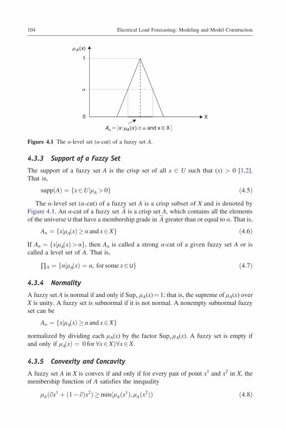
suppðAÞ ¼ fx2UjμA > 0g ð4:5ÞThe α-level set (α-cut) of a fuzzy set A is a crisp subset of X and is denoted by

Figure 4.1. An α-cut of a fuzzy set eA is a crisp set A, which contains all the elementsof the universe ∪ that have a membership grade in eA greater than or equal to α. That is,

Aα ¼ fxjμAðxÞ� α and x2Xg ð4:6ÞIf Aα ¼ fxjμAðxÞ> αg, then Aα is called a strong α-cut of a given fuzzy set A or iscalled a level set of A. That is,

∏A ¼ fαjμAðxÞ ¼ α, for some x2 ∪g ð4:7Þ

4.3.4 Normality

A fuzzy set A is normal if and only if Supx μA(x)¼ 1; that is, the supreme of μA(x) overX is unity. A fuzzy set is subnormal if it is not normal. A nonempty subnormal fuzzyset can be

Aα ¼ fxjμAðxÞ� α and x2Xgnormalized by dividing each μA(x) by the factor Supx μA(x). A fuzzy set is empty ifand only if μAðxÞ ¼ 0 for ∀x2XÞ∀x2X.

4.3.5 Convexity and Concavity

A fuzzy set A in X is convex if and only if for every pair of point x1 and x2 in X, themembership function of A satisfies the inequality

μAð∂x1 þ ð1� ∂Þx2Þ�minðμAðx1Þ, μAðx2ÞÞ ð4:8Þ

0

1

�A (x)

X

A� � Hx ��A (x ) � � and x � X J

�

Figure 4.1 The α-level set (α-cut) of a fuzzy set A.


where ∂2 [0,1] (see Figure 4.2). Alternatively, a fuzzy set is convex if all α-level setsare convex.

Dually, A is concave if its complement Ac is convex. It is easy to show that if A andB are convex, so is A ∩B. Dually, if A and B are concave, so is A ∪B.

4.3.6 Basic Operation

This section provides a summary of some basic set-theoretic operations that areuseful in fuzzy mathematical programming and fuzzy multiple-objectivedecision making. These operations are based on the definitions from Bellman andZadeh [1].

1. InclusionLet A and B be two fuzzy subsets of X. Then A is included in B if and only if

Aα ¼ fxjμAðxÞ� α and x2XgμAðxÞ� μBðxÞ for ∀x2X ð4:9Þ

2. EqualityA and B are called equal if and only if

μAðxÞ ¼ μBðxÞ for ∀x2X ð4:10Þ

3. ComplementationA and B are complementary if and only if

μAðxÞ ¼ 1� μBðxÞ for ∀x2X ð4:11Þ

4. IntersectionThe intersection of A and B may be denoted by A ∩ B, which is the largest fuzzy subsetcontained in both fuzzy subsets A and B. When the min operator is used to express the logi-cal “and,” its corresponding membership is then characterized by

μA∩BðxÞ ¼ minðμAðxÞ, μBðxÞÞ for ∀x2X

¼ μAðxÞ∧ μBðxÞð4:12Þ

where ∧ is a conjunction.

1

0

�A (x)

�A (x1)

�A (�x1� (1��) x2)

�A (x2)

X1 X2X

Figure 4.2 A convex fuzzy set.


5. UnionThe union (A ∪ B) of A and B is dual to the notion of intersection. Thus, the union of A andB is defined as the smallest fuzzy set containing both A and B.

The membership function of A ∪ B is given by

μA∪BðxÞ ¼ maxðμAðxÞ, μBðxÞÞ for ∀x2X¼ μAðxÞ∨μBðxÞ ð4:13Þ

6. Algebraic ProductThe algebraic product AB of A and B is characterized by the following membershipfunction:

μA∪BðxÞ ¼ μAðxÞ μBðxÞ for ∀x2X ð4:14Þ

7. Algebraic SumThe algebraic sum A ⊕ B of A and B is characterized by the following membershipfunction:

μA⊕BðxÞ ¼ μAðxÞ þ μBðxÞ� μAðxÞμBðxÞ ð4:15Þ

8. DifferenceThe difference A�B of A and B is characterized by

μA∩BcðxÞ ¼ minðμAðxÞ, μBcðxÞÞ ð4:16Þ9. Fuzzy Arithmetic

a. Addition of Fuzzy NumbersThe addition of X and Y can be calculated by using α-level cut and max-min convolution.α-level cut. Using the concept of confidence intervals, the α-level sets of X and Y areXα ¼ XL

α , XUα

� �and Yα ¼ YL

α , YUα

� �, where the result, Z, of the addition is

Zα ¼ XαðþÞYα ¼ XLα þ YL

α ,XUα þ YU

α

� � ð4:17Þ

for every α2 [0, 1].Max-min convolution. The addition of the fuzzy numbers X and Y is represented as

ZðzÞ ¼ maxz¼xþy

�min½ μXðxÞ, μYðyÞ�

� ð4:18Þ

b. Subtraction of Fuzzy Numbersα-level cut. The subtraction of the fuzzy numbers X and Y in the α-level cut representa-tion is

Zα ¼ Xαð�ÞYα ¼ XLα � YU

α ,XUα � YL

α

� � ð4:19Þ

for every α2 [0,1].Max-min convolution. The subtraction of the fuzzy numbers X and Y is represented as

μZðZÞ ¼ maxz¼x� y

f μxðxÞ, μYðyÞ½ �gmaxz¼xþy

μxðxÞ, μYð�yÞ½ �f gmaxz¼xþy

f μxðxÞ, μ�YðyÞ½ �gð4:20Þ


c. Multiplication of Fuzzy Numbersα-level cut. The multiplication of the fuzzy numbers X and Y in the α-level cut represen-tation is

Zα ¼ Xαð.ÞYα ¼�XLαy

Lα , X

Uα Y

Uα

� ð4:21Þ

for every α2 [0,1].Max-min convolution. The multiplication of the fuzzy numbers X and Y is representedby Kaufmann and Gupta [2] in the following procedure as1. Find Z1 (the peak of the fuzzy number Z) such that μZðz1Þ ¼ 1; then calculate the left

and right legs.2. The left leg of μZ (z) is defined as

μzðzÞ ¼ maxxy� z

fmin½ μxðxÞ, μYðyÞ�g ð4:22Þ

3. The right leg of μZ (z) is defined as

μzðzÞ ¼ maxxy� z

fmin½ μxðxÞ, μYðyÞ�g ð4:23Þ

d. Division of Fuzzy Numbersα-level cut. The division is represented as follows:

Zα ¼ Xαð:ÞYα ¼�xLα=y

Uα , x

Uα =y

Lα

� ð4:24Þ

Max-min convolution. As defined earlier, we must find the peak and then the left andright legs:1. The peak Z¼X (:) Y is used.2. The left leg is presented as

μzðzÞ ¼ maxx=y� z

fmin½ μxðxÞ, μYðyÞ�gmaxxy� z

fmin½ μxðxÞ, μYð1=yÞ�gmaxxy� z

fmin½ μxðxÞ, μ1=YðyÞ�gð4:25Þ

3. The right leg is presented as

μzðzÞ ¼ maxx=y� z

fmin½ μxðxÞ, μYðyÞ�gmaxxy� z

fmin½ μxðxÞ, μYð1=yÞ�gmaxxy� z

fmin½ μxðxÞ, μ1=YðyÞ�gð4:26Þ

10. LR-Type Fuzzy NumberA fuzzy number is defined to be of the LR type if there are reference functions L and R andpositive scalars, as shown in Figure 4.3, α (left spread), β (right spread), and m (mean),such that

μMðxÞ ¼L

m� x

α

� �for x�m

Rx�m

β

� �for x�m

8>><>>:9>>=>>; ð4:27Þ


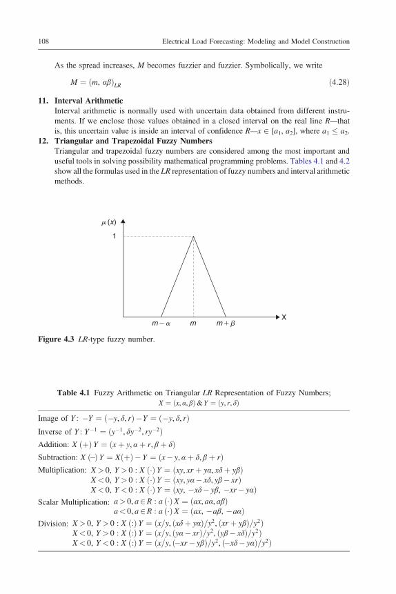
As the spread increases, M becomes fuzzier and fuzzier. Symbolically, we write

M ¼ ðm, αβÞLR ð4:28Þ

11. Interval ArithmeticInterval arithmetic is normally used with uncertain data obtained from different instru-ments. If we enclose those values obtained in a closed interval on the real line R—thatis, this uncertain value is inside an interval of confidence R—x 2 [a1, a2], where a1 � a2.

12. Triangular and Trapezoidal Fuzzy NumbersTriangular and trapezoidal fuzzy numbers are considered among the most important anduseful tools in solving possibility mathematical programming problems. Tables 4.1 and 4.2show all the formulas used in the LR representation of fuzzy numbers and interval arithmeticmethods.

1

� (x)

Xm � � m � �m

Figure 4.3 LR-type fuzzy number.

Table 4.1 Fuzzy Arithmetic on Triangular LR Representation of Fuzzy Numbers;X ¼ x, α, βð Þ&Y ¼ y, r, δð Þ

Image of Y : �Y ¼ �y, δ, rð Þ�Y ¼ �y, δ, rð ÞInverse of Y : Y�1 ¼ ðy�1, δy�2, ry�2ÞAddition: X þð ÞY ¼ xþ y, αþ r, β þ δð ÞSubtraction: X �ð Þ Y ¼ X þð Þ� Y ¼ x� y, αþ δ, β þ rð ÞMultiplication: X> 0, Y > 0 : X �ð Þ Y ¼ xy, xr þ yα, xδþ yβð Þ

X< 0, Y > 0 : X �ð Þ Y ¼ xy, yα� xδ, yβ� xrð ÞX< 0, Y < 0 : X �ð Þ Y ¼ xy, �xδ� yβ, �xr� yαð Þ

Scalar Multiplication: a> 0, a2R : a �ð ÞX ¼ ax, aα, aβð Þa< 0, a2R : a �ð ÞX ¼ ax, �aβ, �aαð Þ

Division: X> 0, Y > 0 : X :ð Þ Y ¼ x=y, xδþ yαð Þ=y2, xr þ yβð Þ=y2ð ÞX< 0, Y > 0 : X :ð Þ Y ¼ x=y, yα� xrð Þ=y2, yβ� xδð Þ=y2ð ÞX< 0, Y < 0 : X :ð Þ Y ¼ x=y, �xr� yβð Þ=y2, �xδ� yαð Þ=y2ð Þ


4.4 Fuzzy Linear Estimation

The fuzzy parameters linear estimation model or fuzzy regression model can bedescribed by the following equation [3–13]:

Y ¼ fðx,AÞ ¼ A1x1 þ A2x2 þ A3x3 þ . . .þ Anxn ð4:29Þ

At any observation j; j¼ 1,2, . . . ,m, equation (4.29) can be rewritten as

Yj ¼ fðx,AÞ ¼ A1x1j þ A2x2j þ A3x3j þ . . .þ Anxnj ð4:30Þ

In fuzzy regression, the difference between the observed and estimated values isassumed to be due to the ambiguity inherently present in the system. Therefore,the preceding fuzzy regression model is built in terms of the possibility and evaluatesall observed values as possibilities that the system should contain. The model inequation (4.29) is named as a possible regression model. In this model Yj is the obser-vation measurement j. This output observation may be a nonfuzzy or fuzzy observa-tion; Ai, i¼ 1,2, . . . ,n are the fuzzy parameters of the model in the form of (pi, ci),where pi is the middle and ci is the spread. Or, it may take the form of the LRtype as ðpi, cLi , cRi Þ, and xij is the input to the model i¼ 1, 2, . . . ,n and j¼ 1,2, . . . ,m.In this section, three cases for the output Yj are studied.

4.4.1 Nonfuzzy Output (Yj¼mj)

In the nonfuzzy output model, the output Yj is a nonfuzzy observation, but the modelcoefficients Ai, i¼ 1,2, . . . ,n are fuzzy parameters either in the form of Ai¼ (pi, ci) or,Ai ¼ pi, cLi , c

Ri

� , i¼ 1, . . . ,n for the LR type and the input xij is a nonfuzzy input. The

membership functions for each type of Ai are shown in Figures 4.4 and 4.5.

Table 4.2 Fuzzy Interval Arithmetic on Triangular Fuzzy Numbers;X ¼ xm, xp, xoð Þ&Y ¼ ym, yp, yoð Þ

Image of Y: �Y ¼ �ym, �yo, �ypð ÞInverse of Y: Y�1 ¼ ð1=ym, 1=yo, 1=ypÞAddition: X þð ÞY ¼ xm þ ym, xp þ yp, xo þ yoð ÞSubtraction: X �ð ÞY ¼ X þð Þ� Y ¼ xm � ym, xp � yo, xo � ypð ÞMultiplication: X> 0, Y > 0 : X �ð Þ Y ¼ xmym, xpyp, xoyoð Þ

X< 0, Y > 0 : X �ð Þ Y ¼ xmym, xpyo, xoypð ÞX< 0, Y < 0 : X �ð Þ Y ¼ xmym, xoyo, xpypð Þ

Scalar Multiplication: a> 0, a2R : a �ð ÞX ¼ axm, axp, axoð Þa< 0, a2R : a �ð ÞX ¼ axm, axo, axpð Þ

Division: X> 0, Y > 0 : X :ð ÞY ¼ xm=ym, xp=yo, xo=ypð ÞX< 0, Y > 0 : X :ð ÞY ¼ xm=ym, xo=yo, xp=ypð ÞX< 0, Y < 0 : X :ð ÞY ¼ xm=ym, xo=yp, xp=yoð Þ


The equation that describes this membership can be written mathematically, for thetriangular fuzzy number, as

μA ¼ 1� jpj � aijcj

; pj � cj � ai� pj þ cj

0 otherwise

8<: ð4:31Þ

where the membership function of Aj of the LR type is assumed to be a trapezoidalfunction, as shown in Figure 4.5. Note that if b2¼ b3, we obtain the triangular mem-bership. In general, the membership function for the LR type can be described as

μA ¼L pj � x

cLj

!for x� pj

R pj � x

cRj

!for x� pj

8>>>>><>>>>>:ð4:32Þ

� (A)

ci cIpi A i

1

0

Figure 4.4 Membership functions of the fuzzy coefficients Aj.

� (A)

b1 b2 b3 b4 A1

1

0

Figure 4.5 Trapezoidal membership function of Aj.


where pi is the middle or the mean of Aj, cLj is the left spread, and cRi is the rightspread.

Equation (4.29) can now be written as

Yj ¼ ðp1, c1Þx1j þ ðp2, c2Þx2j þ ðpn, cnÞxnj, j ¼ 1, 2, . . . ,m ð4:33Þfor the first type of the fuzzy parameters and

Yj ¼ ðp1, cL1, cR1 Þx1j þ ðp2, cL2, cR2 Þx2j þ ðpn, cLn , cRn Þxnj, j ¼ 1, 2, . . . ,m,

ð4:34Þfor the second type of the fuzzy parameters.

In the nonfuzzy output data regression described by equations (4.33) and (4.34),we seek to find the coefficients Ai¼ (pi, ci) or Ai ¼ ðPi, cLi , c

Ri Þ that minimize the

spread of the fuzzy output for all data sets. In mathematical form, this can bedescribed as

Minimize

J1 ¼Xmj¼1

Xni¼1

cixij ð4:35Þ

such that the fuzzy regression model could contain all observed data in the estimatedfuzzy numbers resulting from the model. This can be expressed mathematically as

yj �Xni¼1

pixij �ð1� λÞXni¼1

cixij ð4:36Þ

yj �Xni¼1

pixij þ ð1� λÞXni¼1

cixij ð4:37Þ

Note that the first term on the right side of equations (4.36) and (4.37) representsthe estimated middle of the fuzzy coefficients, whereas the second term represents theestimated spread of these coefficients and λ is the level of fuzziness and is specifiedby the user.

For the fuzzy coefficients of the LR type, the cost function to be minimized isMinimize

J1 ¼Xmj¼1

Xni¼1

2mj � 2pjxij þ cLi xij � cRi xij� ð4:38Þ

subject to satisfying the following two constraints on each data point

yj �Xni¼1

pixij �ð1� λÞXni¼1

cLi xji, j ¼ 1, . . . , . . . , m ð4:39Þ

yj �Xni¼1

pixij þ ð1� λÞXni¼1

cLi xji, j ¼ 1, . . . , . . . ,m ð4:40Þ


The problems formulated in equations (4.35), (4.36), and (4.37) and formulated inequations (4.38), (4.39), and (4.40) are linear optimization problems, which can besolved by the well-known linear programming–based simplex method. However, ifthe sum of the absolute value deviations in equations (4.35) and (4.38) is to be mini-mized, subject to satisfying the inequality constraints given by equations (4.36) and(4.37) and equations (4.39) and (4.40), then the problem turns out to be one of theleast absolute value linear optimization problems and can be solved by using the soft-ware package RLAV available in the IMSL/STAT library.

4.4.2 Fuzzy Output Systems

If the output is fuzzy, in this case it may be represented by a fuzzy number in the formYj¼ (mj, αj) in the case of a triangular fuzzy number (TFN) or Yj ¼ ðmj, αLj , α

Rj Þ,

j¼ 1, 2, . . . ,m in the case of a trapezoidal membership function. For the TFN mem-bership function, equation (4.30) can be written as

Yj ¼ ðmj, αjÞ ¼ ðp1, c1Þx1j þ ðp2, c2Þx2j þ ðpn, cnÞxnj j ¼ 1, 2, . . . ,m

ð4:41Þwhich can be rewritten as

ðmj, αjÞ ¼ ðp1x1j þ p2x2j þ . . .þ pnxnj, c1x1j þ c2x2j þ cnxnjÞ, j ¼ 1, 2, . . . ,m

ð4:42Þ

ðmj, αjÞ ¼Xni¼1

pixij,Xni¼1

cixij

!ð4:43Þ

Equation (4.43) is valid when

mj ¼Xni¼1

pixij j ¼ 1, 2, . . . ,m ð4:44Þ

αj ¼Xni¼1

cixij j ¼ 1, 2, . . . ,m ð4:45Þ

The problem now turns out to be as follows: Given the fuzzy output Yj¼ (mj, αj),the task is to find the fuzzy parameters (pi, ci), i¼ 1, 2, . . . ,n that minimize the costfunction given by

J1ðpi, ciÞ ¼Xmj¼1

mj �Xni¼1

pixij þ αj �Xni¼1

cixij

! ð4:46Þ


subject to satisfying the following constraints on each measurement point:

mj �ð1� λÞαj �Xni¼1

pixij �Xni¼1

cixij j ¼ 1, 2, . . . , n ð4:47Þ

mj þ ð1� λÞαj �Xni¼1

pixij þXni¼1

cixij j ¼ 1, 2, . . . , n ð4:48Þ

If the fuzzy output is of the LR type, then equation (4.42) can be rewritten as

ðmj, αLj , β

Rj Þ ¼

Xni¼1

pixij,Xni¼1

cLi xij,Xni¼1

cRi xij

!ð4:49Þ

Equation (4.49) can be separated into the following equations:

mj ¼Xni¼1

pixij j ¼ 1, . . . , . . . , . . . ,m ð4:50Þ

αLj ¼Xni¼1

cLi xij j ¼ 1, . . . , . . . , . . . ,m ð4:51Þ

βRj ¼Xni¼1

cRi xij j ¼ 1, . . . , . . . , . . . ,m ð4:52Þ

In this case, the objective function to be minimized is given as

J1 ¼ 14

Xni¼1

4mj � 4Xni¼1

pixxj � αLj þXni¼1

cLi xxj � βRj �Xni¼1

cRi xij

" # ð4:53Þ

subject to satisfying the following constraints:

mj �ð1� λÞcLj �Xni¼1

pixij �Xni¼1

cLi xij, j ¼ 1, 2, . . . , n ð4:54Þ

mj þ ð1� λÞcRj �Xni¼1

pixij þXni¼1

cRj xij, j ¼ 1, 2, . . . , n ð4:55Þ

Again, the problems formulated in equations (4.46), (4.47), and (4.48) and thoseformulated in equations (4.53), (4.54), and (4.55) for LR type are all linear optimiza-tion problems subjected to a set of linear constraints. These problems can be solvedusing the standard linear programming–based simplex method. However, if the objec-tive functions are the minimization of the sum of the absolute value of the deviation,then the least absolute value optimization technique based on linear programmingis used to solve the problems formulated here.


Example 4.1

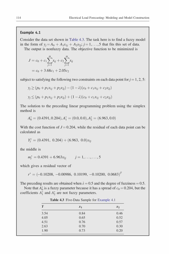
Consider the data set shown in Table 4.3. The task here is to find a fuzzy modelin the form of yj¼A0 þ A1x1j þ A2x2j; j¼ 1, . . . , 5 that fits this set of data.

The output is nonfuzzy data. The objective function to be minimized is

J ¼ c0 þ c1Xmj¼1

xij þ c2Xmj¼1

xij

¼ c0 þ 3:68c1 þ 2:05c2

subject to satisfying the following two constraints on each data point for j¼ 1, 2, 5:

yj �ðp0 þ p1x1j þ p2x2jÞ� ð1� λÞðc0 þ c1x1j þ c2x2jÞ

yj �ðp0 þ p1x1j þ p2x2jÞ þ ð1� λÞðc0 þ c1x1j þ c2x2jÞ

The solution to the preceding linear programming problem using the simplexmethod is

A�0 ¼ ð0:4391, 0:204Þ,A�

1 ¼ ð0:0, 0:0Þ,A�2 ¼ ð6:963, 0:0Þ

With the cost function of J¼ 0.204, while the residual of each data point can becalculated as

Yj� ¼ ð0:4391, 0:204Þ þ ð6:963, 0:0Þx2j

the middle is

mj� ¼ 0:4391þ 6:963x2j j ¼ 1, . . . , . . . , 5

which gives a residual vector of

r� ¼ ð�0:10208, �0:00986, 0:10199, �0:10200, 0:0683ÞT

The preceding results are obtained when λ¼ 0.5 and the degree of fuzziness¼ 0.5.Note that A�

0 is a fuzzy parameter because it has a spread of c0¼ 0.204, but thecoefficients A�

1 and A�2 are not fuzzy parameters.

Table 4.3 Five-Data Sample for Example 4.1

Y x1 x2

3.54 0.84 0.464.05 0.65 0.524.51 0.76 0.572.63 0.70 0.301.90 0.73 0.20


Example 4.2

In a fuzzy regression, the output y is a TFN with cj representing the error. Thefuzzy output and the corresponding crisp input are given as:

where λ¼ 0.4 determines the fuzzy coefficients for a simple model Yj¼A0þ A1xj.Because the output is a fuzzy number of TFN memberships, then the cost

function to be minimized is

J ¼X2j¼1

ðmj �ðp0 þ p1x1jÞ þ αj �ðc0 þ c1x1jÞÞ

¼ 7:25�ðp0 þ p1x1jÞ

Because the first term is a constant one, the cost function to be minimized is

J ¼ �ðp0 þ p1x1j þ c0 þ c1x1jÞ

subject to satisfying the following constraints:

mj � 0:6αj �ðp0 þ p1x1jÞ� ðc0 þ c1x1jÞ, j ¼ 1, 2

mj þ 0:6αj �ðp0 þ p1x1jÞ þ ðc0 þ c1x1jÞ, j ¼ 1, 2

Substituting the preceding data given we obtain

0:9� p0 þ 0:52p1 � c0 � 0:52c1

4:39� p0 þ 1:36p1 � c0 � 1:36c1

2:22� p0 þ 0:52p1 þ c0 þ 0:52c1

4:81� p0 þ 1:36p1 þ c0 þ 1:36c1

Using the linear programming–based simplex method approach, we obtain thefollowing solution:

A�0 ¼ ð2:855, 1:955Þ, A�

1 ¼ ð0:0, 0:0Þ

where J¼ 2.44 and the residual vector of the inequality constraint is

r� ¼ ð0:0, �3:49, �2:59, 0:00ÞT

This indicates that the obtained solution is valid.

( yi, ci) xi

(2.1, 0.2) 0.52(4.6, 0.35) 1.36


Example 4.3

This example is for the LR type; the solution obtained was based on minimumleast absolute deviation. The data for the TFN fuzzy output are listed in Table 4.4.

The model required to fit these data points is in the form

Yj ¼ A0 þ A1xj þ A1x2j , j ¼ 1, . . . , . . . , 16

The cost function to be minimized in this case is given as

J ¼ 0:25X16j¼1

4mj � αLj þ βRj

� �� 0:25½ð4p0 þ 96p1 þ 148:4p2

� cL0 � 24cL1 � 96:6cL2 þ cR0 þ 24cR1 þ 96:6cR2 Þ�As mentioned earlier, if the first term of J is constant, then the cost function to beminimized is

J1 ¼ �0:25 4p0 þ 96p1 þ 148:4p2 � cL0 � 24cL1 � 96:6cL2 þ cR0��

þ 24cR1 þ 96:6cR2 Þ�subject to satisfying the inequality constraints given as

mj �ð1� λÞcLj � p0 þ p1x1j þ p2x22j

� �� cL0 þ cL1x1j þ cL2x

22j

� �,

j ¼ 1, . . . , . . . , 16

mj þ ð1� λÞcLj � p0 þ p1x1j þ p2x22j

� �þ cL0 þ cL1x1j þ cL2x

22j

� �,

j ¼ 1, . . . , . . . , 16

Note that, the number of parameters to be estimated is 9 and the number ofinequality constraints is 32. The solution to the fuzzy parameters for the pro-posed model has been found to be

A0 ¼ ð12:75, 2:75, 0:0Þ, A1 ¼ ð42:1, 0, 0Þ, and

A2 ¼ ð140:794, 144:3, 0:0ÞTable 4.4 Data for Example 4.3

No. xj Yj ¼ (mj, αLj , βRj ) No. xj Yj ¼ (mj, αLj , β

Rj )

1 0.0 (11.5, 3, 2.5) 9 1.6 (84., 15., 16.)2 0.2 (24.8, 4.5, 4.) 10 1.8 (82., 15., 16.)3 0.4 (40. 6., 7.) 11 2.0 (103.7, 16., 17.)4 0.6 (45.2, 7., 7.) 12 2.2 (102.6, 16., 17.)5 0.8 (49.1, 9. 9.) 13 2.4 (103.1, 16., 17.)6 1.0 (70. 11. 12.) 14 2.6 (111., 17., 19.)7 1.2 (70.9, 12. 12.) 15 2.8 (109., 17. 19.)8 1.4 (80.1, 14. 15.) 16 3.0 (121.7, 18. 21.)


with an alarm from the linear program that this solution is not the uniquesolution. The model equation in this case can be written as

Y ¼ ð12:75, 2:75, 0:0Þ þ ð42:1, 0, 0Þxþ ð140:794, 144:3, 0:0Þx2

This model satisfies all the constraints on the fuzzy optimization problem formu-lated previously. In the next section, we offer an example for the electrical loadestimation.

Example 4.4

The fuzzy linear parameter estimation algorithm, proposed in the preceding sec-tions, is implemented for determination of the required distribution system underuncertain conditions [18]. The uncertainty appears at input, at output, and in thenature of the system itself. Measured data are given in Table 4.5, where Er is theyearly energy consumption, Pi is the installed capacity of electrical equipment atcustomers’ sites, and Pr is the yearly peak load.

The task is to build a fuzzy linear model that relates the yearly energy con-sumption Er and Pr in the form of

Pr ¼ A0 þ ArEr

or

Pr ¼ ðp0, c0Þ þ ðp1, c1ÞEr

Table 4.5 Power Measured at a Substation for Example 4.4

# Er (MWh) Pi (kW) Pr (kW)

1 21.79 125 30.2 60.20 247 27.93 60.72 436 40.54 65.01 406 39.65 70.00 265 42.06 70.55 251 29.27 72.30 520 42.08 79.05 540 42.09 80.39 310 30.9

10 114.0 443 57.011 114.45 573 57.512 125.00 438 37.213 148.00 578 55.514 162.10 610 59.6


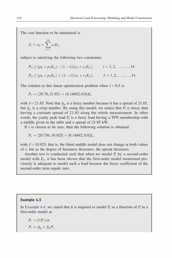
The cost function to be minimized is

J1 ¼ c0 þX14j¼1

c1Eir

subject to satisfying the following two constraints:

Pri �ðp0 þ p1EirÞ� ð1:�λÞðc0 þ c1EirÞ, i ¼ 1, 2, . . . , . . . , 14

Pri �ðp0 þ p1EirÞ þ ð1:�λÞðc0 þ c1EirÞ, I ¼ 1, 2, . . . , . . . , 14

The solution to this linear optimization problem when λ¼ 0.5 is

Pr ¼ ð29:76, 21:85Þ þ ð0:14692, 0:0ÞEr

with J¼ 21.85. Note that A0 is a fuzzy number because it has a spread of 21.85,but A1 is a crisp number. By using this model, we notice that Pr is fuzzy datahaving a constant spread of 21.85 along the whole measurement. In otherwords, the yearly peak load Pr is a fuzzy load having a TFN membership witha middle given in the table and a spread of 21.85 kW.

If λ is chosen to be zero, then the following solution is obtained:

Pr ¼ 29:756, 10:925½ � þ 0:14692, 0:0½ �Er

with J¼ 10.925; that is, the fitted middle model does not change at both valuesof λ, but as the degree of fuzziness decreases, the spread decreases.

Another test is conducted such that when we model Pr by a second-ordermodel with Er, it has been shown that the first-order model mentioned pre-viously is adequate to model such a load because the fuzzy coefficient of thesecond-order term equals zero.

Example 4.5

In Example 4.4, we stated that it is required to model Pr as a function of Pi in afirst-order model as

Pr ¼ f ðPiÞ orPr ¼ A0 þ A1Pi


The cost function to be minimized in this case, according to the data available inTable 4.5, is

J1 ¼ c0 þ 5742 ci

subject to satisfying the following two constraints on the measurement set:

Prj �ð p0 þ p1PijÞ� ð1:� λÞðc0 þ c1PijÞ, j ¼ 1, 2, . . . , . . . , 14

Prj �ð p0 þ p1PijÞ þ ð1:� λÞðc0 þ c1PijÞ, j ¼ 1, 2, . . . , . . . , 14

The results obtained in this test for λ¼ 0.5 are

Pr ¼ ð25:78, 19:6813Þ þ ð0:0483, 0:0ÞPi

with J¼ 19.6813. It has been found that such a model is adequate for these data,and a higher-order model gives zero fuzzy coefficients.

If the yearly peak load Pr is presented as a function of Er and Pi as

Pr ¼ A0 þ A1Er þ A2Pi

then the cost function to be minimized in this case is

J ¼ c0 þ 1243:56c1 þ 5742c2

subject to satisfying

ðPrÞj � p0 þ p1ðErÞj þ p2ðPiÞj �ð1� λÞðc0 þ c1ðErÞj þ c2ðPiÞjÞ,j ¼ 1, . . . , . . . , 14

ðPrÞj � p0 þ p1ðErÞj þ p2ðPiÞj þ ð1:� λÞðc0 þ c1ðErÞj þ c2ðPiÞjÞ,j ¼ 1, . . . , . . . , 14

The solution to the preceding optimization problem at λ¼ 0.5 is

Pr ¼ ð25:51, 15:59Þ þ ð0:0027, 0:00ÞEr þ ð0:0483, 0:0ÞPi

with J¼ 19.59. Note that A0 is a fuzzy number with a spread of 19.59 and that Pris a fuzzy number with a spread¼ 19.59.


Example 4.6

The yearly peak load in the preceding example is given as an LR type, as shownin Table 4.6 [18]. The task is to model this load as

Ps ¼ A0 þ ArEr

where A0 ¼ p0, cL0, cR0

� and A1 ¼ p1, cL1, c

R1

� .

Using the cost function defined in equation (4.53) and the constraints definedin equations (4.54) and (4.55), for this linear model, we obtain the followingresults:

Ps ¼ ð0:0, 0:0, 0:0Þ þ ð2:134, 1:974, 0:0ÞEr

Now, the spread of Pr at a given measurement j, is

cLs , cRs

� ¼ 1:974Er, 0:0ð Þj j ¼ 1, . . . , . . . , 14

while the middle is

ðmsÞj ¼ ð2:134ErÞj j ¼ 1, . . . , . . . , 14

4.5 Fuzzy Short-Term Load Modeling

Most of the work on offline short-term load models available today assumes that theparameters of the model are constant crisp values [14–19]. This assumption is, tosome extent, true, as long as there are no big changes in weather parameters fromday to day. The load power is characterized by both uncertainty and ambiguity.

Table 4.6 Samples of Measurements in SS for Example 4.6

# Er (MWh) Pi (kW) Pr (kW)

1 21.79 125 (30, 25, 33)2 60.20 247 (27.9, 24, 30.5)3 60.72 436 (40.5, 34.8, 44.9)4 65.01 406 (39.6, 36.1, 43)5 70.00 265 (42.0, 38, 45.7)6 70.55 251 (29.2, 26, 33)7 72.30 520 (42.0, 37.6, 45)8 79.05 540 (42.0, 38.5, 46)9 80.39 310 (30.9, 27, 34.5)

10 114.0 443 (57.0, 52.5, 60.9)11 114.45 573 (57.5, 52.8, 61.4)12 125.00 438 (37.2, 34.4, 40.8)13 148.00 578 (55.5, 52, 59.8)14 162.10 610 (59.6, 55.3, 64.7)


In this section, the load models used in Chapter 3 are reformulated to account forfuzziness of the load characteristics. In the first subsection the input is assumed to becrisp, whereas the load model parameters are expressed as fuzzy numbers having acertain middle and spreads. Three models are used in this section—namely, fuzzyload models A, B, and C. Fuzzy load model A is a multiple linear regressionmodel. This model takes into account the weather parameters. Fuzzy load model Bis a harmonic model and does not account for the weather parameters. Fuzzy loadmodel C is a hybrid model that combines models A and B and takes into accountthe weather parameters.

In this section we assume that the input data are fuzzy numbers having certainmiddles and spreads. The parameters of the load model are fuzzy. The fuzzy numbersused for the fuzzy variables in this section are assumed to have a symmetrical trian-gular membership function.

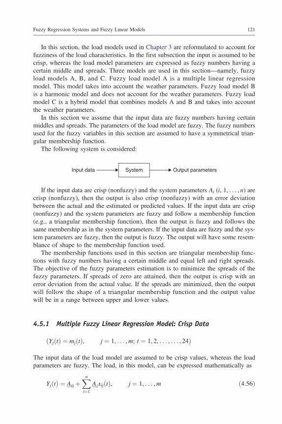
The following system is considered:

If the input data are crisp (nonfuzzy) and the system parameters Ai (i, 1, . . . ,n) arecrisp (nonfuzzy), then the output is also crisp (nonfuzzy) with an error deviationbetween the actual and the estimated or predicted values. If the input data are crisp(nonfuzzy) and the system parameters are fuzzy and follow a membership function(e.g., a triangular membership function), then the output is fuzzy and follows thesame membership as in the system parameters. If the input data are fuzzy and the sys-tem parameters are fuzzy, then the output is fuzzy. The output will have some resem-blance of shape to the membership function used.

The membership functions used in this section are triangular membership func-tions with fuzzy numbers having a certain middle and equal left and right spreads.The objective of the fuzzy parameters estimation is to minimize the spreads of thefuzzy parameters. If spreads of zero are attained, then the output is crisp with anerror deviation from the actual value. If the spreads are minimized, then the outputwill follow the shape of a triangular membership function and the output valuewill be in a range between upper and lower values.

4.5.1 Multiple Fuzzy Linear Regression Model: Crisp Data

ðYjðtÞ ¼ mjðtÞ, j ¼ 1, . . . ,m; t ¼ 1, 2, . . . , . . . , 24Þ

The input data of the load model are assumed to be crisp values, whereas the loadparameters are fuzzy. The load, in this model, can be expressed mathematically as

YjðtÞ ¼ A0 þXni¼1

AixijðtÞ, j ¼ 1, . . . ,m ð4:56Þ

Input data System Output parameters


where

Yj(t) is the value of the load power at time t;A0 is the fuzzy base load having a triangular membership with a middle p0 and spread c0, asshown in Figure 4.6(a);Ai are the fuzzy coefficients having a triangular membership with a middle pi and spread ci,as shown in Figure 4.6(b).

Equation (4.56) can be rewritten as

YjðtÞ ¼ ðpyjðtÞ, cyjðtÞÞ ¼ mjðtÞ ¼ ðp0, c0Þ þXni¼1

ðpi, ciÞ xijðtÞ ð4:57Þ

As shown earlier in this chapter, for the output data described by equation (4.57), thecoefficients A0 (p0, c0) and Ai (pi, ci) are to be found such that the spread of the fuzzyoutput is minimized for all data sets. In mathematical form, this can be described as

Minimize

J ¼Xt

c0 þXmj¼1

Xni¼1

cixijðtÞ( )

ð4:58Þ

where t 2 0, tF½ �, tF is the number of days for which data are taken at the hour in ques-tion. The fuzzy regression model in equation (4.58) contains all observed data in theestimated fuzzy numbers resulting from the model. This can be expressed mathema-tically as

yjðtÞ � p0 þXni¼1

pixijðtÞ" #

� ð1� λÞ c0 þXni¼1

cixijðtÞ" #

; j ¼ 1, . . . ,m

ð4:59Þ

and

yjðtÞ� p0 þXni¼1

pixijðtÞ" #

þ ð1� λÞ c0 þXni¼1

cixijðtÞ" #

; j ¼ 1, . . . ,m ð4:60Þ

Note that the first term on the right side of equations (4.59) and (4.60) representsthe estimated middle of the fuzzy coefficients, and the second term represents the esti-mated spread of these coefficients. λ is the level of fuzziness and is specified by theuser. As λ increases, the fuzziness of the output increases. In the preceding equations,m is the number of observations, and n is the number of fuzzy parameters used inthe model.

In the following subsections, two multiple fuzzy linear regression models aredeveloped. The first model can be used to predict the load during the winter season,whereas the second model can be used to predict the load during the summer season.The only difference between the two models is that the winter model considers the


wind-cooling factor as an explanatory variable, and the summer model considers thehumidity factor as an explanatory variable.

4.5.1.1 Fuzzy Load Model A: Winter Model

The fuzzy winter model, in Chapter 3, equation (3.12), can be rewritten in fuzzyform as

YjðtÞ ¼ A0 þ A1TjðtÞ þ A2T2j ðtÞ þ A3T

3j ðtÞ þ A4Tjðt� 1Þ þ A5Tjðt� 2Þ

þ A6Tjðt� 3Þ þ A7WjðtÞ þ A8Wjðt� 1Þ þ A9Wjðt� 2Þ; j ¼ 1, . . . ,m

ð4:61Þ

where Yj(t) is the load power j; j ¼ 1, . . . ,m at time t; t ¼ 1, 2, . . . , 24 and is assumedto be given as nonfuzzy data. Tj(t) is the jth temperature deviation from nominal at

� (A)

ci cIpi A i

1

0

(a)

(b)

� (A)

ci cIpi Ai

1

0

Figure 4.6 (a) Membership function of A0; (b) membership function of AI.


time t and is given by equation (3.13). Wj(t) is the wind-cooling factor at time t and isgiven by equation (3.15), and A0, A1, . . . , A9 are load model fuzzy coefficients hav-ing middles p0, p1, . . . , p9 and spreads c0, c1, . . . , c9.


YjðtÞ ¼ ðp0, c0Þ þ ðp1, c1ÞTjðtÞ þ ðp2, c2Þ T2j ðtÞ þ ðp3, c3Þ T3

j ðtÞþ ðp4, c4ÞTjðt� 1Þ þ ðp5, c5ÞTjðt� 2Þ þ ðp6, c6ÞTjðt� 3Þþ ðp7, c7ÞWjðtÞ þ ðp8, c8ÞWjðt� 1Þ þ ðp9, c9ÞWjðt� 2Þ;j ¼ 1, . . . ,m

ð4:62Þ

In fuzzy linear regression, the spreads of the fuzzy coefficients are to be mini-mized. This results in an objective function that can be expressed mathematically as

J ¼Xt

c0þXmj¼1

c1TjðtÞþ c2T2j ðtÞþ c3T

3j ðtÞþ c4Tjðt�1Þ

h(:

þ c5Tjðt�2Þc6Tjðt�3Þþ c7WjðtÞþ c8WjðtÞðt�1Þþ c9Wjðt�2Þi) ð4:63Þ

where t 2 0, tF½ �, tF is the number of days for which data are taken at the hour inquestion. This is subject to satisfying the two inequality constraints on each loadpower given as

yjðtÞ�p0þp1TjðtÞþp2T2j ðtÞþp3T

3j ðtÞþp4Tjðt�1Þþp5Tjðt�2Þ

þp6Tjðt�3Þþp7WjðtÞþp8Wjðt�1Þþ p9Wjðt�2Þ�ð1�λÞðc0þ c1TjðtÞþ c2T

2j ðtÞþ c3T

3j ðtÞþ c4Tjðt�1Þþ c5Tjðt�2Þþ c6Tjðt�3Þ

þ c7WjðtÞþ c8Wjðt�1Þþ c9Wjðt�2ÞÞ, j¼ 1,2, . . . ,m

ð4:64Þ

yjðtÞ� p0 þ p1TjðtÞ þ p2T2j ðtÞ þ p3T

3j ðtÞ þ p4Tjðt� 1Þ þ p5Tjðt� 2Þ

þ p6Tjðt� 3Þ þ p7WjðtÞ þ p8Wjðt� 1Þ þ p9Wjðt� 2Þþ ð1� lÞðc0 þ c1TjðtÞ þ c2T

2j ðtÞ þ c3 T

3j ðtÞ þ c4Tjðt� 1Þ

þ c5Tjðt� 2Þ þ c6Tjðt� 3Þ þ c7WjðtÞ þ c8Wjðt� 1Þþ c9Wjðt� 2ÞÞ, j ¼ 1, 2, . . . ,m

ð4:65Þ

The optimization problem formulated in equations (4.63) to (4.65) is linear and can besolved using linear programming based on the simplex method available in the IMSL/STAT library.

Having identified the middle and spread of each coefficient, we can then obtain thefuzzy load model for the winter season using equation (4.61) or equation (4.62).


4.5.1.2 Fuzzy Load Model A: Summer Model

The summer fuzzy model for short-term load forecasting can be written as

YðtÞ ¼ A0 þ A1 TðtÞ þ A2T2ðtÞ þ A3T

3ðtÞ þ A4Tðt� 1Þ þ A5Tðt� 2Þþ A6Tðt� 3Þ þ A7HðtÞ þ A8Hðt� 1Þ þ A9Hðt� 2Þ ð4:66Þ

where

Y ðtÞ is the summer load power at time t;T(t) is the temperature deviation at time t given by equation (3.13) in Chapter 3;A0, A1, . . . , A9 are the fuzzy load coefficients having a certain middle p0, p1, . . . , p9 andcertain spread c0, c1, . . . , c9 at time t;H(t) is the temperature humidity factor given by equation (3.17) in Chapter 3.

The summer load model stated in equation (4.66) takes into account the tempera-ture deviation and the temperature humidity factor for each hour and at three and twohours before.


YjðtÞ ¼ ðp0, c0Þ þ ðp1, c1Þ TjðtÞ þ ðp2, c2Þ T2j ðtÞ þ ðp3, c3Þ T3

j ðtÞþ ðp4, c4Þ Tjðt� 1Þ þ ðp5, c5Þ Tjðt� 2Þ þ ðp6, c6Þ Tjðt� 3Þþ ðp7, c7ÞHjðtÞ þ ðp8, c8ÞHjðt – 1Þ þ ðp9, c9ÞHjðt� 2Þ

ð4:67Þ

In fuzzy linear regression, the parameters Ai ¼ (pi, ci), i ¼ 1, . . . , . . . , 9 are to befound that minimize the spread of the fuzzy output for all data sets. This can beexpressed mathematically as

Minimize

J ¼Xt

c0 þXmj¼1

c1TjðtÞþ c2T2j ðtÞþ c3T

3j ðtÞþ c4Tjðt�1Þ

h(þc5Tjðt�2Þþ c6Tjðt�3Þþ c7HjðtÞþ c8Hjðt�1Þþ c9Hjðt�2Þ

i)ð4:68Þ

where t 2 0, tF½ �, tF is the number of days for which data are taken at the hour in ques-tion. This is subject to satisfying the following inequality constraints at j; j¼ 1, . . . ,m:



þ p6Tjðt� 3Þ þ p7HjðtÞ þ p8Hjðt� 1Þ þ p9Hjðt� 2Þ� ð1� λÞ�c0 þ c1TjðtÞ þ c2T

2j ðtÞ þ c3T

3j ðtÞ þ c4Tjðt� 1Þ þ c5Tjðt� 2Þ:

þ c6Tjðt� 3Þ þ c7HjðtÞ þ c8Hjðt� 1Þ þ c9Hjðt� 2Þ�, j ¼ 1, 2, . . . ,m

ð4:69Þ




þ p6Tjðt� 3Þ þ p7HjðtÞ þ p8Hjðt� 1Þ þ p9Hjðt� 2Þ� ð1� λÞ�c0 þ c1TjðtÞ þ c2T

2j ðtÞ þ c3T

3j ðtÞ þ c4Tjðt� 1Þ þ c5Tjðt� 2Þ:

þ c6Tjðt� 3Þ þ c7HjðtÞ þ c8Hjðt� 1Þ þ c9Hjðt� 2Þ�, j ¼ 1, 2, . . . ,m

ð4:70Þ

The problem formulated in equations (4.68) to (4.70) is linear and can be solved bythe linear programming optimization package available in the IMSL/STAT library.

Having obtained the fuzzy parameters Ai ¼ ðpi, ciÞ, i ¼ 1, . . . , 9, we can then pre-dict the load for the next 24 hours using equation (4.67).

4.5.1.3 Fuzzy Load Model B

Fuzzy load model B is a harmonic decomposition model and does not account forweather conditions. It does not account for temperature deviation, wind-cooling fac-tor, or humidity factor. Thus, this model can be used for both winter and summersimulations.

The fuzzy load at any time t, therefore, can be written as

YðtÞ ¼ A0 þXni¼1

ðAi sin iωt þ Bi cos iωtÞ ð4:71Þ

where

Y ðtÞ is the load power at time t and it is assumed to have crisp values;A0, Ai, and Bi are fuzzy parameters having certain middles and spreads and are given asA0 ¼ ðp0, c0Þ, Ai ¼ ðpi, ciÞ, and Bi ¼ ðai, biÞ.The model described in equation (4.71) can be rewritten as

YðtÞ ¼ ðp0, c0Þ þXni¼1

ðpi, ciÞ sin iωt þ ðαi, biÞ cos iωt½ � ð4:72Þ

Note that the middles and the spreads are constants and are estimated seven timesweekly.

The objective is to find the fuzzy parameters that minimize the spread of the loadpower. Mathematically, this can be written as

Minimize

J ¼Xt

c0 þXmj¼1

Xni¼1

cixijðtÞ þ biyijðtÞ� �( )

ð4:73Þ

where

xijðtÞ ¼ ðsin iωtÞj, j ¼ 1, . . . ,m; i ¼ 1, . . . , n;yijðtÞ ¼ ðcos iωtÞj, j ¼ 1, . . . ,m; i ¼ 1, . . . , n;


m, n are the number of observations and harmonics chosen in the model, respectively;t 2 0, tF½ �, tF is the number of days for which data are taken at the hour in question.

This is subject to satisfying the inequality constraints given by


ðpi sin iωt þ αi cos iωtÞ" #

j

�ð1� λÞ c0 þXni¼1

ðci sin iωt þ bi cos iωtÞj" # ð4:74Þ


ðpi sin iωt þ αi cos iωtÞ" #

j

þ ð1� λÞ c0 þXni¼1

ðci sin iωt þ bi cos iωtÞj" # ð4:75Þ

The optimization problem formulated in equations (4.73) to (4.75) is a linear optimi-zation problem and can be solved using the simplex method of linear programming.

Having obtained the fuzzy load parameters, we can then predict the load for thenext 24 hours using equation (4.72).

4.5.1.4 Fuzzy Load Model C

Fuzzy load model C is a fuzzy hybrid model that takes into account weather-dependentcomponents. The base load in the model is a time-varying function and takes the formof Fourier’s coefficients. This model can be considered as a combination of fuzzyload model A and fuzzy load model B. Here, the weather input is limited only to tem-perature deviation, and the model is used for both winter and summer load forecastsimulations.

The fuzzy load model in this case can be written mathematically as

YjðtÞ ¼ A0 þXni¼1

Ai sin iωt þ Bi cos iωt½ �( )

j

þ C0TjðtÞ þ C1Tjðt� 1Þ þ C2Tjðt� 2Þ þ C3Tjðt� 3Þ� � ð4:76Þ

where

A0, Ai, Bi and are the weather-independent fuzzy parameters having certain middles andcertain spreads;C0, C1, C2, andC3 are the temperature-dependent fuzzy parameters.

The terms in the first brace in equation (4.76) canbe considered as the base load,whichdepends only on time, whereas the terms in the second brace are the temperature-dependent load terms.



YðtÞ ¼ ðp0, c0Þ þXni¼1

½ðpi, αiÞxiðtÞ þ ðbi, βiÞ yiðtÞ� þ ½ðγo, s0ÞTjðtÞ

þ ðγ1, s1Þ Tjðt� 1Þ þ ðγ2, s2Þ Tjðt� 2Þ þ ðγ3, s3Þ Tjðt� 3Þ�ð4:77Þ

In equation (4.77), the first letter in the parameter’s brackets indicates the middle ofthat parameter, and the second letter indicates the spread of this parameter.

In fuzzy regression, the fuzzy model parameters are to be found to minimize thespread of the output. In mathematical form, this can be expressed as

J ¼Xt

c0 þXmj¼1

Xni¼1

½αixijðtÞ þ βiyijðtÞ� þXmj¼1

½s0TjðtÞ þ s1Tjðt� 1Þ(

þ s2Tjðt� 2Þ þ s3Tjðt� 3Þ�)

ð4:78Þ

where t 2 0, tF½ �, tF is the number of days for which data are taken at the hour inquestion.

This is subject to satisfying the following two constraints on the output so thatthe fuzzy regression model could contain all the observed data j, j ¼ 1, . . . , min the estimated fuzzy numbers resulting from the model. This can be expressedmathematically as


ðpixijðtÞ þ biyijðtÞ þ γ0TjðtÞ þ γ1Tjðt� 1Þ þ γ2Tjðt� 2Þ"

þ γ3Tjðt� 3ÞÞ#– ð1� λÞ c0 þ

Xni¼1

ðαixijðtÞ þ βiyijðtÞÞ þ s0TjðtÞ"

þ s1Tjðt� 1Þ þ s2Tjðt� 2Þ þ s3Tjðt� 3Þ#, j ¼ 1, . . . ,m

ð4:79Þ


ðpixijðtÞ þ biyijðtÞ þ γ0TjðtÞ þ γ1Tjðt� 1Þ þ γ2Tjðt� 2Þ"

þ γ3Tjðt� 3ÞÞ#þ ð1� λÞ c0 þ

Xni¼1

ðαixijðtÞ þ βiyijðtÞÞ þ s0TjðtÞ"

þ s1Tjðt� 1Þ þ s2Tjðt� 2Þ þ s3Tjðt� 3Þ#, j ¼ 1, . . . ,m

ð4:80ÞThe problem formulated in equations (4.78) to (4.80) is a linear optimization problemand can be solved using linear programming based on the simplex method explained


earlier in this chapter. Having identified the fuzzy model parameters, we can predictthe load for the next 24 hours using equation (4.77).

4.5.2 Multiple Fuzzy Linear Regression Model: Fuzzy Data

In Section 4.5, the load power data are assumed to be nonfuzzy, whereas the parametersof the load power are fuzzy. Different linear optimization problems were derived withdifferent load models. In this section, the load data are assumed to be fuzzy powervalues having a certain middle and certain spread Y jðtÞ ¼ ½mjðtÞ, αjðtÞ�, where mj(t)is the middle of the load power at the time t in question during the observation j,and αj(t) is the spread of the load power at time t and observation j. Using this formula-tion of fuzzy numbers means that a triangular membership function is assumed, asshown in Figures 4.6(a) and (b).

The fuzzy model for the load power can be expressed mathematically as

YjðtÞ ¼ ½mjðtÞ, αjðtÞ� ¼ A0 þXni¼1

AixijðtÞ, j ¼ 1, . . . ,m ð4:81Þ

which can be rewritten as

½mjðtÞ, αjðtÞ� ¼ ðp0, c0Þ þXni¼1

ðpi, ciÞ xijðtÞ, j ¼ 1, . . . ,m ð4:82aÞ

Alternatively, it can be separated as

½mjðtÞ, αjðtÞ� ¼ p0 þXni¼1

pixijðtÞ( )

, c0 þXni¼1

ci xijðtÞ( )" #

, j ¼ 1, . . . ,m

ð4:82bÞEquation (4.82b) is valid only when: Given two fuzzy numbers M1 ¼

ðm1, α1, β1ÞLR and M2 ¼ ðm2, α2, β2ÞLR in terms of LR functions [2] that followtriangular membership function, where:

m1 and m2 are the centers of the membership function;α1 and α2 are left-side spreads;β1 and β2 are right-side spreads.

Then

M1ðm1, α1, β1ÞLR þ M2ðm2, α2, β2ÞLR ¼ ðms, αs, βsÞLRwhere

ms ¼ m1 þ m2

αs ¼ α1 þ α2

βs ¼ β1 þ β2

The center of the sum is equal to the sum of the centers, and each spread of thesum is the sum of its respective spread.


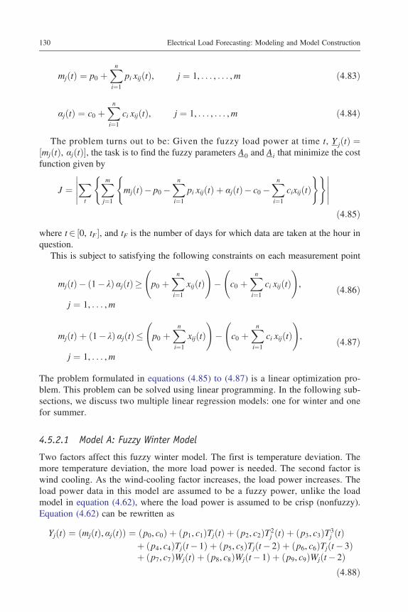
mjðtÞ ¼ p0 þXni¼1

pi xijðtÞ, j ¼ 1, . . . , . . . ,m ð4:83Þ

αjðtÞ ¼ c0 þXni¼1

ci xijðtÞ, j ¼ 1, . . . , . . . ,m ð4:84Þ

The problem turns out to be: Given the fuzzy load power at time t, Y jðtÞ ¼½mjðtÞ, αjðtÞ�, the task is to find the fuzzy parameters A0 and Ai that minimize the costfunction given by

J ¼Xt

Xmj¼1

mjðtÞ� p0 �Xni¼1

pi xijðtÞ þ αjðtÞ� c0 �Xni¼1

cixijðtÞ( )( )

ð4:85Þ

where t 2 0, tF½ �, and tF is the number of days for which data are taken at the hour inquestion.

This is subject to satisfying the following constraints on each measurement point

mjðtÞ � ð1� λÞ αjðtÞ � p0 þXni¼1

xijðtÞ !

� c0 þXni¼1

ci xijðtÞ !

,

j ¼ 1, . . . ,m

ð4:86Þ

mjðtÞ þ ð1� λÞ αjðtÞ� p0 þXni¼1

xijðtÞ !

� c0 þXni¼1

ci xijðtÞ !

,

j ¼ 1, . . . ,m

ð4:87Þ

The problem formulated in equations (4.85) to (4.87) is a linear optimization pro-blem. This problem can be solved using linear programming. In the following sub-sections, we discuss two multiple linear regression models: one for winter and onefor summer.

4.5.2.1 Model A: Fuzzy Winter Model

Two factors affect this fuzzy winter model. The first is temperature deviation. Themore temperature deviation, the more load power is needed. The second factor iswind cooling. As the wind-cooling factor increases, the load power increases. Theload power data in this model are assumed to be a fuzzy power, unlike the loadmodel in equation (4.62), where the load power is assumed to be crisp (nonfuzzy).Equation (4.62) can be rewritten as

YjðtÞ ¼ ðmjðtÞ, αjðtÞÞ ¼ ðp0, c0Þ þ ðp1, c1ÞTjðtÞ þ ðp2, c2ÞT2j ðtÞ þ ðp3, c3ÞT3

j ðtÞþ ðp4, c4ÞTjðt� 1Þ þ ðp5, c5ÞTjðt� 2Þ þ ðp6, c6ÞTjðt� 3Þþ ðp7, c7ÞWjðtÞ þ ðp8, c8ÞWjðt� 1Þ þ ðp9, c9ÞWjðt� 2Þ

ð4:88Þ



mjðtÞ ¼ p0 þ p1TjðtÞ þ p2T2j ðtÞ þ p3T


þ p6Tjðt� 3Þ þ p7WjðtÞ þ p8Wjðt� 1Þ þ p9Wjðt� 2Þ,j ¼ 1, . . . ,m

ð4:89Þ

αjðtÞ ¼ c0 þ c1TjðtÞ þ c2T2j ðtÞ þ c3T

3j ðtÞ þ c4Tjðt� 1Þ þ c5Tjðt� 2Þ

þ c6Tjðt� 3Þ þ c7WjðtÞ þ c8Wjðt� 1Þ þ c9Wjðt� 2Þ,j ¼ 1, . . . ,m

ð4:90Þ

Given the fuzzy load power (mj(t), αj(t)) at any time t, the task is to determine themiddle and the spread of each parameter that minimizes the cost function

J ¼X

t

Xmj¼1

½mjðtÞ� fp0 þ p1TjðtÞ þ p2T2j ðtÞ þ p3T

3j ðtÞ þ p4Tjðt� 1Þ

þ p5Tjðt� 2Þ þ p6Tjðt� 3Þ þ p7WjðtÞ þ p8Wjðt� 1Þ þ p9Wjðt� 2Þgþ αjðtÞ� fc0 þ c1TjðtÞ þ c2T

2j ðtÞ þ c3T

3j ðtÞ þ c4Tjðt� 1Þ þ c5Tjðt� 2Þ

þ c6Tjðt� 3Þ þ c7WjðtÞ þ c8Wjðt� 1Þ þ c9Wjðt� 2Þg�

ð4:91Þwhere t 2 0, tF½ �, and tF is the number of days for which data are taken at the hour inquestion.

This is subject to satisfying the following two constraints at eachmeasurement point:

mjðtÞ� ð1� λÞ αjðtÞ� ½ðRHS of equation 4:89Þ� ðRHS of equation 4:90Þ�,j ¼ 1, . . . ,m

ð4:92Þ

mjðtÞ þ ð1� λÞ αjðtÞ� ½ðRHS of equation 4:89Þ þ ðRHS of equation 4:90Þ�,j ¼ 1, . . . ,m

ð4:93Þwhere RHS stands for right-hand side.

The problem formulated in equations (4.91) to (4.93) is one of linear optimization.This problem can be solved using standard linear programming.

Having identified the fuzzy parameters of the fuzzy winter model, we can predictthe load in a winter day. The middle of the load can be predicted at any hour t usingequation (4.89), and the spread can be predicted using equation (4.90).

4.5.2.2 Model A: Fuzzy Summer Model

The load in the fuzzy summer model is a function of the temperature deviation andhumidity factor. The load power and the load model parameters are assumed to befuzzy numbers. Mathematically, this can be expressed as


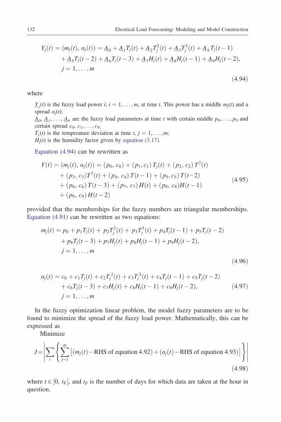
YjðtÞ ¼ ðmjðtÞ, αjðtÞÞ ¼ A0 þ A1TjðtÞ þ A2T2j ðtÞ þ A3T

3j ðtÞ þ A4 Tjðt� 1Þ

þ A5Tjðt� 2Þ þ A6Tjðt� 3Þ þ A7HjðtÞ þ A8Hjðt� 1Þ þ A9Hjðt� 2Þ,j ¼ 1, . . . ,m

ð4:94Þ

where

Y j(t) is the fuzzy load power i; i ¼ 1, . . . ,m, at time t. This power has a middle mj(t) and aspread αj(t);A0, A1, . . . , A9 are the fuzzy load parameters at time t with certain middle p0, . . . , p9 andcertain spread c0, c1, . . . , c9;Tj (t) is the temperature deviation at time t, j ¼ 1, . . . ,m;Hj(t) is the humidity factor given by equation (3.17).


YðtÞ ¼ ðmjðtÞ, αjðtÞÞ ¼ ðp0, c0Þ þ ðp1, c1Þ TjðtÞ þ ðp2, c2Þ T2ðtÞþ ðp3, c3ÞT3ðtÞ þ ðp4, c4Þ Tðt� 1Þ þ ðp5, c5Þ Tðt – 2Þþ ðp6, c6Þ Tðt� 3Þ þ ðp7, c7ÞHðtÞ þ ðp8, c8ÞHðt� 1Þþ ðp9, c9ÞHðt� 2Þ

ð4:95Þ

provided that the memberships for the fuzzy numbers are triangular memberships.Equation (4.91) can be rewritten as two equations:

mjðtÞ ¼ p0 þ p1TjðtÞ þ p2T2j ðtÞ þ p3T


þ p6Tjðt� 3Þ þ p7HjðtÞ þ p8Hjðt� 1Þ þ p9Hjðt� 2Þ,j ¼ 1, . . . ,m

ð4:96Þ

αjðtÞ ¼ c0 þ c1TjðtÞ þ c2Tj2ðtÞ þ c3Tj

3ðtÞ þ c4Tjðt� 1Þ þ c5Tjðt� 2Þþ c6Tjðt� 3Þ þ c7HjðtÞ þ c8Hjðt� 1Þ þ c9Hjðt� 2Þ,j ¼ 1, . . . ,m

ð4:97Þ

In the fuzzy optimization linear problem, the model fuzzy parameters are to befound to minimize the spread of the fuzzy load power. Mathematically, this can beexpressed as

Minimize

J¼Xt

Xmj¼1

ðmjðtÞ�RHS of equation 4:92ÞþðαjðtÞ�RHS of equation 4:93Þ� �( )

ð4:98Þwhere t 2 0, tF½ �, and tF is the number of days for which data are taken at the hour inquestion.


This is subject to satisfying the following constraints:

mjðtÞ� ð1� λÞ αjðtÞ� ½ðRHS of equation 4:92Þ� ðRHS of equation 4:93Þ�,j ¼ 1, . . . ,m

ð4:99Þ

mjðtÞ þ ð1� λÞ αjðtÞ� ½ðRHS of equation 4:92Þ þ ðRHS of equation 4:93Þ�,j ¼ 1, . . . ,m

ð4:100Þ

The optimization problem formulated in equations (4.98) to (4.100) is one of linearoptimization and can be solved using linear programming.

Having obtained the fuzzy load parameters, we then can use equation (4.91) to pre-dict the fuzzy load power at any hour t in question.

4.5.3 Fuzzy Load Model B

Fuzzy load model B does not account for weather conditions in the load; it can beexpressed as

YjðtÞ ¼ ðmjðtÞ, αjðtÞÞ ¼ A0

Xni¼1

½ðAi sin iωt þ Bi cos iωt�j, j ¼ 1, . . . ,m

ð4:101Þ

The only difference between equation (4.71) and (4.101) is the load power Yj(t) attime t. In (4.71) the load power is assumed to be a crisp value, whereas in (4.101)it is assumed to be a fuzzy value having a middle mj(t) and a spread αj(t). Equation(4.101) can be rewritten as

ðmjðtÞ, αjðtÞÞ ¼ ðp0, c0Þ þXni¼1

½ðpi, ciÞ sin iωtþ ðbi, βiÞ cos iωt�j j¼ 1, . . . ,m

ð4:102Þ

which can be split into

mjðtÞ ¼ p0 þXni¼1

½ðpi sin iωt þ bi cos iωtÞ�j, j ¼ 1, . . . ,m ð4:103Þ

αjðtÞ ¼ c0 þXni¼1

½ci sin iωt þ βi cos iωt�j, j ¼ 1, . . . ,m ð4:104Þ

The task is to find the fuzzy load parameters that minimize the spread of the fuzzyload power. This can be expressed mathematically as


J¼Xt

Xmj¼1

½ðmjðtÞ�RHSof equation4:103þðαjðtÞ�RHSof equation4:104Þ�( )

ð4:105Þ


This is subject to satisfying the following two constraints as

mjðtÞ� ð1� λÞ αjðtÞ� ½RHS of equation 4:103�RHS of equation 4:104�;j ¼ 1, . . . ,m

ð4:106Þ

mjðtÞ þ ð1� λÞ αjðtÞ� ½RHS of equation 4:103þ RHS of equation 4:104�;j ¼ 1, . . . ,m

ð4:107Þ

The problem formulated in equations (4.105) to (4.107) is one of linear optimizationthat can be solved using linear programming. Having identified the middle and thespread of fuzzy parameters, we then can use the harmonic load model described in equa-tion (4.101) to predict the load at any hour t. Note that the load power obtained in thiscase is independent of the weather conditions and depends only on the hour in question.

The next model, model C, combines fuzzy load model A and fuzzy load model B.This model takes weather conditions into account.

4.5.4 Fuzzy Load Model C

Fuzzy load model A derived earlier has the advantage of being weather responsive;the fuzzy coefficients of this model depend on the weather conditions. These condi-tions include temperature deviation and cooling factor.

Fuzzy load model B is weather insensitive. The fuzzy coefficients of this modeldepend only on the time in question.

In this section, the two models A and B are combined into one fuzzy model, C.The resulting fuzzy load model C is weather sensitive. This fuzzy model is suitablefor all weekdays and can be used for both winter and summer load-forecast simula-tions. Its main disadvantage is the assumption that the relation between load andweather is constant throughout the day.

The fuzzy model for the load in this case can be expressed mathematically as

YjðtÞ ¼ ðmjðtÞ, αjðtÞÞ ¼ A0 þXni¼1

ðAi sin iωt þ Bi cos iωtÞ( )

j

þ C0TjðtÞ þ C1Tjðt – 1Þ þ C2Tjðt� 2Þ þ C3Tjðt – 3Þ� �

j,

j ¼ 1, . . . ,m

ð4:108Þ


where

mj(t), αj(t) is the middle and spread of load power j, j ¼ 1, . . . ,m at time t;A0, Ai, and Bi are the weather-independent fuzzy parameters with certain middles andspreads;C0, C1, C2, andC3 are the temperature-dependent fuzzy parameters with certain middlesand spreads.

The left-hand side (LHS) of equation (4.108) is the fuzzy load power. The terms inthe first bracket on the right-hand side (RHS) of equation (4.108) can be considered asthe fuzzy base load, and it depends only on time, whereas the second bracket containsthe temperature-dependent fuzzy load terms.


ðmjðtÞ, αjðtÞÞ ¼ ðp0, c0Þ þXni¼1

½ðpi, θiÞxiðtÞ þ ðbi, βiÞyiðtÞ�( )

j

þ fðγ0, c′0ÞTjðtÞ þ ðγ1, c1ÞTjðt� 1Þ þ ðγ2, c2ÞTjðt� 2Þþ ðγ3, c3ÞTjðt� 3Þgj, j ¼ 1, . . . ,m

ð4:109Þ

For simplicity, let

xiðtÞ ¼ sin iωt, i ¼ 1, . . . , n ð4:110aÞyiðtÞ ¼ cos iωt, i ¼ 1, . . . , n ð4:110bÞ

In equation (4.109), the first letter in all small brackets of the equations indicates themiddle of the parameter, and the second letter indicates the spread of that parameter.A triangular membership is used for each parameter.

In the fuzzy model developed in equation (4.109), the task is to find the fuzzymodel parameters to minimize the spread of the output. Mathematically, the fuzzy lin-ear optimization problem can be expressed as

Minimize

J ¼X

t

Xmj¼1

mjðtÞ� p0þ

Xni¼1

½ pixiðtÞ þ biyiðtÞ�j þ γ0TjðtÞ þ γ1Tjðt� 1Þ

þ γ2Tjðt� 2Þ þ γ3Tjðt� 3Þ�þ αjðtÞ�

�c0 þ

Xni¼1

θixiðtÞ þ βiyiðtÞ

�j

þ c00TjðtÞ þ c1Tjðt� 1Þ þ c2Tj ðt� 2Þ þ c3Tjðt� 3Þ

��ð4:111Þ


Subject to satisfying the following two constraints for each measurement pointgiven as


mjðtÞ� ð1� λÞ αjðtÞ� p0 þ

Xni¼1

f½ pixiðtÞ þ biyiðtÞ�gj

þ γ0TjðtÞ þ γ1Tjðt� 1Þ þ γ2Tjðt� 2Þ þ γ3Tjðt� 3Þ�

� c0 þ

Xni¼1

fθixiðtÞ þ βiyiðtÞ�

j

þ c′0TjðtÞ þ c1Tjðt� 1Þþ c2Tjðt� 2Þ þ c3Tjðt� 3Þ, j ¼ 1, . . . ,m

ð4:112Þ

mjðtÞ þ ð1 – λÞ αjðtÞ� p0 þ

Xni¼1

½ pixiðtÞ þ biyiðtÞ� þ γ0TðtÞ þ γ1Tjðt� 1Þ

þ γ2Tjðt� 2Þ þ γ3Tjðt� 3Þ�

þ c0 þ

Xni¼1

θixiðtÞ þ βiyiðtÞ�

j

þ c′0TjðtÞ þ c1Tjðt� 1Þþc2Tjðt� 2Þþc3Tjðt� 3Þ j ¼ 1, . . . ,m

ð4:113Þ

The problem formulated in equations (4.111) to (4.113) is one of linear optimiza-tion and can be solved by linear programming.

Having obtained the middle and spread of each fuzzy parameters, we can calculatethe load power at any hour in question using equation (4.109).

4.6 Conclusion

This chapter presented a new formulation for fuzzy short-term load-forecasting mod-els. In the first part of the chapter, the load power is considered given as crisp (non-fuzzy) data, while the load model parameters are fuzzy, having certain middles andspreads. The problem turns out to be one of linear optimization.

In the second part of the chapter, the load power is considered to be fuzzy power datahaving certain middles and spreads. Three different fuzzy models—A, B, and C—weredeveloped, and new fuzzy equations were obtained. The resulting optimization problemis linear and can be solved using linear programming.

References

[1] T.J. Ross, Fuzzy Logic with Engineering Applications, McGraw-Hill, New York, 1995.[2] M.E. El-Hawary, Electric Power Applications of Fuzzy Systems, IEEE Press, New York,

1998.


[3] J. Nazarko, W. Zalewski, An application ofthe fuzzy regression analysis to the electricalload estimation, Electrotechnical Conference MELECON ’96, 3, 1563–1566, IEEECatalog #96CH35884, May 13–16, 1996.

[4] H. Tanaka, S. Uejima, K. Asai, Linear regression analysis with fuzzy model, IEEE Trans.Syst. Man Cybern 12 (6) (1982) 903–907.

[5] P.T. Chang, E.S. Lee, Fuzzy least absolute deviations regression based on the ranking offuzzy numbers, IEEE World Congr. Fuzzy Syst. IEEE Proc. 2 (1994) 1365–1369.

[6] J. Watada, Y. Yabuchi, Fuzzy robust regression analysis, IEEE World Congr. Fuzzy Syst.IEEE Proc. 2 (1994) 1370–1376.

[7] R. Alex, P.Z. Wang, A new resolution of fuzzy regression analysis, IEEE Int. Conf. Syst.Man Cybern. 2 (1998) 2019–2021.

[8] H. Ishibuchi, M. Nii, Fuzzy regression analysis by neural networks with non-symmetricfuzzy number weights, IEEE Int. Conf. Neural Networks 2 (1996) 1191–1196.

[9] H. Ishibuchi, M. Nii, Fuzzy regression analysis with non-symmetric fuzzy numbercoefficients and its neural network implementation, Proc. Fifth IEEE Int. Conf. FuzzySyst. 1 (1996) 318–324.

[10] S. Ghoshray, Fuzzy linear regression analysis by symmetric triangular fuzzy number coef-ficients, Proc. IEEE Int. Conf. Intell. Eng. Syst. (1997) 307–313.

[11] M.-S. Yang, C.-M. Ko, On cluster-wise fuzzy regression analysis, IEEE Trans. Syst. Man.Cybern. Part B Cybern. 27 (1) (1997) 1–13.

[12] H. Tanaka, H. Lee, Interval regression analysis by quadratic programming approach, IEEETrans. Fuzzy Syst. 6 (4) (1998) 473–481.

[13] C.J. Huang, C.E. Lin, C.L. Haung, Fuzzy approach for generator maintenance scheduling,Electr. Power Syst. Res. 24 (1992) 31–38.

[14] I.M. Altas, A.M. Sharaf, A fuzzy logic power tracking controller for a photovoltic energyconversion scheme, Electr. Power Syst. Res. 25 (1992) 227–238.

[15] C.S. Chen, J.N. Sheen, Applying fuzzy mathematics to the evaluation of avoided cost for aload management program, Electr. Power Syst. Res. 26 (1993) 117–125.

[16] N. Rajakovic, S. Ruzic, Sensitivity analysis of an optimal short term hydro-thermalschedule, IEEE Trans. Power Syst. 8 (3) (1993) 1235–1241.

[17] R. Kenarangui, A. Seifi, Fuzzy power flow analysis, Electr. Power Syst. Res. 29 (1994)105–109.

[18] J.Y. Fan, J.D. McDonald, A real-time implementation of short-term load forecasting fordistribution power systems, IEEE Trans. Power Syst. 9 (2) (1994) 988–944.

[19] D. Srinivasan, M.A. Lee, Survey of hybrid fuzzy neural approach to electric load forecast-ing, IEEE Int. Conf. Syst. Man Cybern. 5 (1995) 4004–4008.


electrical load forecasting. modeling and model...

Documents