short-term load forecasting using theta method

Short-term load forecasting using Theta method

Grzegorz Dudek1,*

1Czestochowa University of Technology, Electrical Engineering Faculty, 42-200 Czestochowa,

Poland

Abstract. The Theta method attracted the attention of researchers and

practitioners in recent years due to its simplicity and superior forecasting

accuracy. Its performance has been confirmed by many empirical studies

as well as forecasting competitions. In this article the Theta method is

tested in short-term load forecasting problem. The load time series

expressing multiple seasonal cycles is decomposed in different ways to

simplify the forecasting problem. Four variants of input data definition are

considered. The standard Theta method is uses as well as the dynamic

optimised Theta model proposed recently. The performances of the Theta

models are demonstrated through an empirical application using real power

system data and compared with other popular forecasting methods.

1 Introduction

Short-term load forecasting (STLF) plays an important role in power systems and energy

markets as accurate forecasting is beneficial for unit commitment, generation dispatch,

hydro scheduling, hydro-thermal coordination, spinning reserve allocation, and other

electric utility operations. As basic driver of electricity prices the system load should be

forecasted with high accuracy which translates to financial performance of energy

companies and other participants of energy markets.

In the literature, there are numerous methods for STLF which can be roughly

categorized into conventional methods and computational intelligence or machine learning

methods. Machine learning methods use supervised learning to model relationships

between predictors and load on historical data. Some well-known methods belonging to this

category are artificial neural networks [1] and support vector machines [2]. The most

commonly employed conventional approaches are the autoregressive integrated moving

average (ARIMA) and exponential smoothing (ETS). The Theta method of forecasting,

introduced by Assimakopoulos and Nikolopoulos [3], is a special case of simple

exponential smoothing with drift. It is of interest to forecast practitioners because its

simplicity and high accuracy in forecasting time series of various character and different

frequencies. Its power was confirmed in M3-Competition [4], where it performed far better

than the participating advanced methods and expert systems and outperformed the rest of its

competitors, particularly for monthly series and microeconomic data.

* Corresponding author: [email protected]

, 0 2019)E3S Web of Conferences https://doi.org/10.1051/e3sconf /201984010041084 0

PE 20184 (

© The Authors, published by EDP Sciences. This is an open access article distributed under the terms of the CreativeCommons Attribution License 4.0 (http://creativecommons.org/licenses/by/4.0/).

In recent years a lot of work has been done in application of Theta method to real-world

forecasting problems and testing its performance on different time series. For example in

[5] new theoretical formulations for the application of the method on multivariate time

series is proposed. Authors evaluate through simulations the bivariate form of the method

and evaluate it in real macroeconomic and financial time series. In [6] the authors propose a

new hybrid method that utilises the decomposition approach of the Theta method with

nonlinear trends, apply smoothing to the data, and shrinkage approach to seasonal data

instead of classical seasonal decomposition. The results on the M3-Competition data are

very promising in terms of forecast accuracy.

Many researchers' efforts are moving towards optimization of the Theta model. The

weights of Theta lines are searched to reconstruct the original time series from the

individual lines. In [7] an approach is presented for selecting the optimal value of the

weight when a single Theta line is used and formulae for optimal weights when combining

two Theta lines are provided. For optimizing the combination weights of the two Theta

lines in the final forecast in [8] a neural network is applied. A generalization of Theta

model in [9] is provided. The proposed dynamic optimised Theta model is a state space

model that selects the best short-term Theta line optimally and revises the long-term Theta

line dynamically. The superior performance of this model is demonstrated through an

empirical application.

In this work to STLF we apply the Theta method in the standard version and in more

sophisticated dynamic optimised version proposed recently [9]. The Theta method was

designed as a linear model for time series without seasonal variations. In STLF the models

have to face a more difficult task, because the load time series is non-stationary in mean

and variance, expresses nonlinear trend and multiple seasonal cycles. Taking into account

the features of load time series, four variants of the STLF procedures using Theta models

are proposed which differ in input data definition.

The remainder of this paper is organized as follows. Section 2 elaborates standard and

dynamic optimised Theta models. In Section 3 four variants of the STLF procedures are

proposed differing in the definition of the input data on which the models are built. Section

4 describes experimental study on real load data. Some concluding remarks are drawn in

the last section of this paper.

2 Standard and dynamic optimised Theta models

The Theta model [3] is a univariate forecasting method based on modifying the local

curvature of the time series through a coefficient “Theta” (θ ℝ) applied to the second

differences of the data. In result of modification new lines are created having the mean and

slope of the original time series. When Theta coefficient is from the range 0 θ < 1, the

curve deflation is observed (the smaller θ, the larger the deflation degree) and long-term

trends can be identified. In the extreme case where θ = 0 the time series is transformed to a

linear regression line. For θ = 1 we get the original time series. If the Theta coefficient

increases above 1, then the time series is dilated (see Fig. 1) and short-term behaviour is

demonstrated.

The original Theta model leading to the creation of a Theta line Z(θ) is achieved as the

solution of the equation [9]:

ntYZ tt ,...,4,3,)( 22 (1)

where Y1, …, Yn is the original time series, and is the difference operator (i.e. Xt = Xt −

Xt−1).


PE 20184 (

2

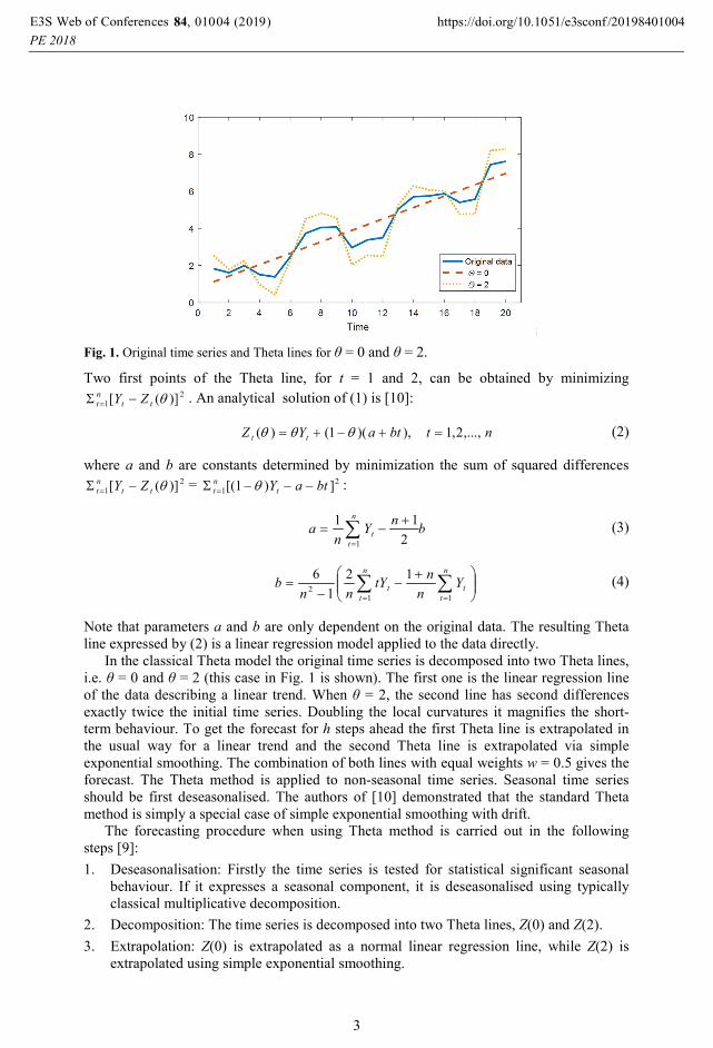
Fig. 1. Original time series and Theta lines for θ = 0 and θ = 2.

Two first points of the Theta line, for t = 1 and 2, can be obtained by minimizing 2

1 )]([ tt

n

t ZY . An analytical solution of (1) is [10]:

ntbtaYZ tt ,...,2,1),)(1()( (2)

where a and b are constants determined by minimization the sum of squared differences 2

1 )]([ tt

n

t ZY = 2

1 ])1[( btaYt

n

t :

bn

Yn

an

t

t

1 2

11 (3)

n

t

n

t

tt Yn

ntY

nnb

1 12

12

1

6 (4)

Note that parameters a and b are only dependent on the original data. The resulting Theta

line expressed by (2) is a linear regression model applied to the data directly.

In the classical Theta model the original time series is decomposed into two Theta lines,

i.e. θ = 0 and θ = 2 (this case in Fig. 1 is shown). The first one is the linear regression line

of the data describing a linear trend. When θ = 2, the second line has second differences

exactly twice the initial time series. Doubling the local curvatures it magnifies the short-

term behaviour. To get the forecast for h steps ahead the first Theta line is extrapolated in

the usual way for a linear trend and the second Theta line is extrapolated via simple

exponential smoothing. The combination of both lines with equal weights w = 0.5 gives the

forecast. The Theta method is applied to non-seasonal time series. Seasonal time series

should be first deseasonalised. The authors of [10] demonstrated that the standard Theta

method is simply a special case of simple exponential smoothing with drift.

The forecasting procedure when using Theta method is carried out in the following

steps [9]:

1. Deseasonalisation: Firstly the time series is tested for statistical significant seasonal

behaviour. If it expresses a seasonal component, it is deseasonalised using typically

classical multiplicative decomposition.

2. Decomposition: The time series is decomposed into two Theta lines, Z(0) and Z(2).

3. Extrapolation: Z(0) is extrapolated as a normal linear regression line, while Z(2) is

extrapolated using simple exponential smoothing.


PE 20184 (

3

4. Combination: The forecast is generated from the extrapolated Z(0) and Z(2) lines by

their combination with equal weights.

5. Reseasonalisation: The forecast is reseasonalised if the original time series was

identified as seasonal in step 1.

The Theta method presented above uses only two Theta lines, but more Theta lines can

be used for modelling and forecasting the original time series in order to extract more

information from the data. The selection of the parameters θ can be optimized to achieve

the lowest forecast errors. Another modification of the classical Theta method is to use of

unequal weights in the recomposition procedure for the final forecasts. In such a case the

two Theta lines are combined as follows [9]:

)()1()( 21 ttt ZwwZY (5)

where w [0, 1].

Assuming than θ1 < 1 and θ2 1, the weight can be derived as w = (θ2 – 1) / (θ2 – θ1). So, it

is dependent on θ–parameters. If we fix θ1 = 0 and searching for the optimal value of

θ2 = θ > 1, the weight is of the form: w = 1/θ.

Parameters a and b, defined by (3) and (4), respectively, are fixed for all t. In [9] they

are considered as dynamic functions, i.e. at state t parameters at and bt are updated from the

historical time series Y1, …, Yt. In such a case the model can be expressed by a state space

model (see derivation in [9]):

tttY (6)

11

1

1

)1(1)1(

11 t

t

t

t

tt bal

(7)

1)1( ttt lYl (8)

ttt bt

Ya2

1 (9)

)(

6)2(

1

111 tttt YY

tbt

tb (10)

])1[(1

1 ttt YYtt

Y (11)

where t = 1, 2, …, n, lt ℝ is the level parameter, [0, 1] is the smoothing parameter,

and 1 represents θ2 (θ1 is assumed to be 0).

The initial values of the states are assumed to be a0 = b0 = b1 = 0Y = 0 as in [9]. The

parameters: l0, and are estimated by minimising the sum of squared error:

n

t

ttl

Yl1

2

,,0 )(minarg)ˆ,ˆ,ˆ(

0

(12)

For the forecast horizon h 2 the forecasts are generated recursively. The model is

called dynamic optimised Theta model (DOTM). Note that due to dynamic functions at and

bt the model is nonlinear.


PE 20184 (

4

3 STLF using Theta models

Load time series usually express multiple seasonal variations: annual, weekly and daily

ones. A trend and stochastic irregular component is also present. The noise level in a load

time series depends on the system size and the customer structure, as well as a trend, and

amplitudes of the annual, weekly and daily cycles. In STLF we focus on a daily profile. It

changes over the year and depends on the day of the week.

Taking into account the features of load time series, four variants of the forecasting

procedures are proposed differing in the definition of the input data on which the models

are built. The first variant v1 bases on the original time series having both daily and weekly

variations. Other variants are composed of the hourly loads selected from the original time

series so as to simplify the input data, i.e. to remove weekly (v2), daily (v3) or both

seasonality (v4). The four variants are:

v1 – The forecasting model generates forecasts for the next day (24 hours) in the recursive

manner. The input data is the load time series including m previous days, so the length

of the time series on which Theta model is built is n = 24m (assuming hourly load

time series). In the experimental part of this work m is set to 21 days, so n = 504 data

points. In such case input data series expresses daily and weekly seasonality (three

weeks). Annual seasonality is not expressed in such short time series fragment.

v2 – As in version v1, the forecasting model generates forecasts for the next day hour by

hour in the recursive manner. The input data is the load time series composed of p

days of the same type as the forecasted day (Monday, …, Sunday) from the history.

That is, when the forecasted day is Monday, the input time series includes

concatenated profiles for p Mondays preceding the forecasted day. In the experimental

part of the work p is set to 7, so n = 247 = 168 data points.

v3 – The forecasting model generates forecasts for hour h of the next day. The input data is

the load time series composed of loads at hour h of n previous days. With such a

definition of the input time series, the daily seasonality was eliminated. Input time

series expresses weekly seasonality. In the experimental part of the work n is set to 21

days, so three weekly cycles are observed in the input data. For forecasting load at

hours h = 1, 2, …, 24 of the next day, twenty four Theta models are built.

v4 – As in version v3, the forecasting model generates forecasts for hour h of the next day.

The input data is the load time series composed of loads at hour h of n previous days

of the same type as the forecasted day (Monday, …, Sunday). For example, when the

forecasted day is Monday and the forecasted hour is h, the input time series includes

loads at our h of n Mondays preceding the forecasted day. In the experimental part of

the work n is set to 7. Such definition of the input data eliminates all seasonal

components. In this variant, for forecasting load at hours h = 1, 2, …, 24 of the next

day, twenty four Theta models are built.

The input time series are visualized in Fig. 2. Note that the Theta models are facing

different forecasting problems in versions v1–v4. In variant v1 the input time series

expresses full information about time series including daily and weekly seasonality. The

model has to deal with the complex data to generate the forecast. In variant v2 we simplify

input data eliminating weekly variation. Thanks to this, we expect an improvement in the

forecast accuracy. Data in variant v3 are also simplified having only weekly seasonality and

only 21 points, instead of 168 as in v2 or 504 as in v1. The most simplified input data,

without any seasonality and having only 7 points, are in variant v4. But note that in variant

v1 and v2 we build one model for forecasting 24 values of the daily pattern. The models

work in the recursive manner. While in variants v3 and v4 we build 24 models generating

forecasts for individual hours of the day. In the simulation study we compare the models

accuracy.


PE 20184 (

5

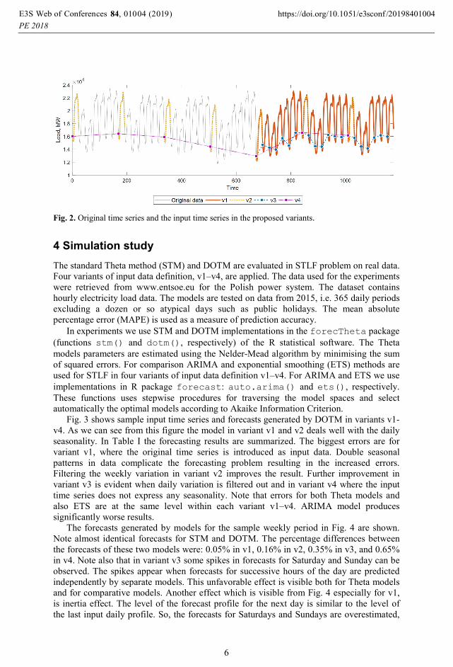
Fig. 2. Original time series and the input time series in the proposed variants.

4 Simulation study

The standard Theta method (STM) and DOTM are evaluated in STLF problem on real data.

Four variants of input data definition, v1–v4, are applied. The data used for the experiments

were retrieved from www.entsoe.eu for the Polish power system. The dataset contains

hourly electricity load data. The models are tested on data from 2015, i.e. 365 daily periods

excluding a dozen or so atypical days such as public holidays. The mean absolute

percentage error (MAPE) is used as a measure of prediction accuracy.

In experiments we use STM and DOTM implementations in the forecTheta package

(functions stm() and dotm(), respectively) of the R statistical software. The Theta

models parameters are estimated using the Nelder-Mead algorithm by minimising the sum

of squared errors. For comparison ARIMA and exponential smoothing (ETS) methods are

used for STLF in four variants of input data definition v1–v4. For ARIMA and ETS we use

implementations in R package forecast: auto.arima() and ets(), respectively.

These functions uses stepwise procedures for traversing the model spaces and select

automatically the optimal models according to Akaike Information Criterion.

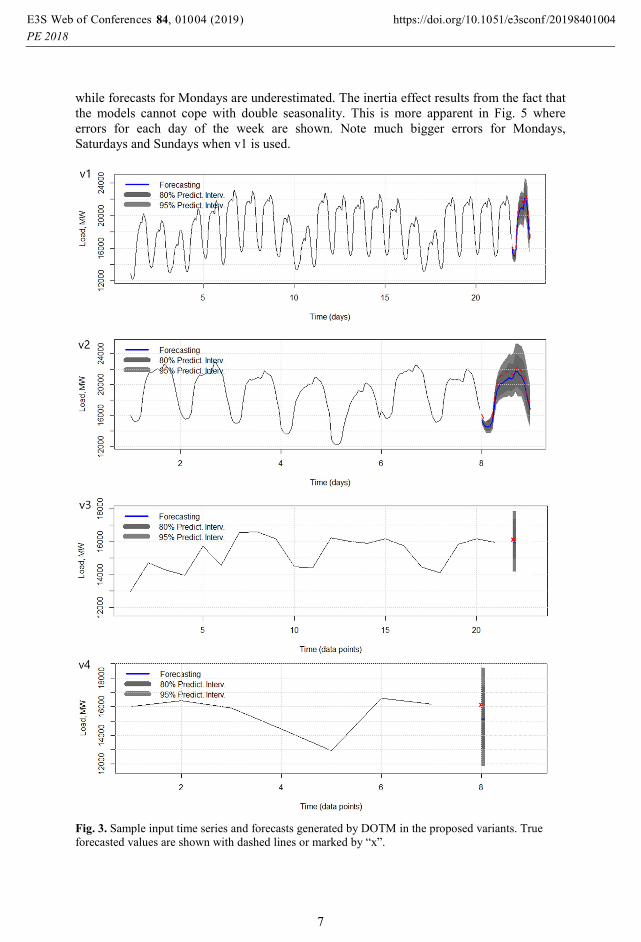
Fig. 3 shows sample input time series and forecasts generated by DOTM in variants v1-

v4. As we can see from this figure the model in variant v1 and v2 deals well with the daily

seasonality. In Table I the forecasting results are summarized. The biggest errors are for

variant v1, where the original time series is introduced as input data. Double seasonal

patterns in data complicate the forecasting problem resulting in the increased errors.

Filtering the weekly variation in variant v2 improves the result. Further improvement in

variant v3 is evident when daily variation is filtered out and in variant v4 where the input

time series does not express any seasonality. Note that errors for both Theta models and

also ETS are at the same level within each variant v1–v4. ARIMA model produces

significantly worse results.

The forecasts generated by models for the sample weekly period in Fig. 4 are shown.

Note almost identical forecasts for STM and DOTM. The percentage differences between

the forecasts of these two models were: 0.05% in v1, 0.16% in v2, 0.35% in v3, and 0.65%

in v4. Note also that in variant v3 some spikes in forecasts for Saturday and Sunday can be

observed. The spikes appear when forecasts for successive hours of the day are predicted

independently by separate models. This unfavorable effect is visible both for Theta models

and for comparative models. Another effect which is visible from Fig. 4 especially for v1,

is inertia effect. The level of the forecast profile for the next day is similar to the level of

the last input daily profile. So, the forecasts for Saturdays and Sundays are overestimated,


PE 20184 (

6

while forecasts for Mondays are underestimated. The inertia effect results from the fact that

the models cannot cope with double seasonality. This is more apparent in Fig. 5 where

errors for each day of the week are shown. Note much bigger errors for Mondays,

Saturdays and Sundays when v1 is used.

Fig. 3. Sample input time series and forecasts generated by DOTM in the proposed variants. True

forecasted values are shown with dashed lines or marked by “x”.


PE 20184 (

7

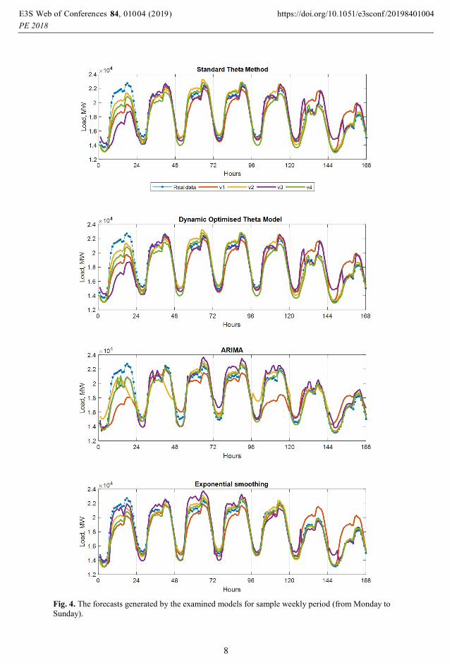
Fig. 4. The forecasts generated by the examined models for sample weekly period (from Monday to

Sunday).


PE 20184 (

8

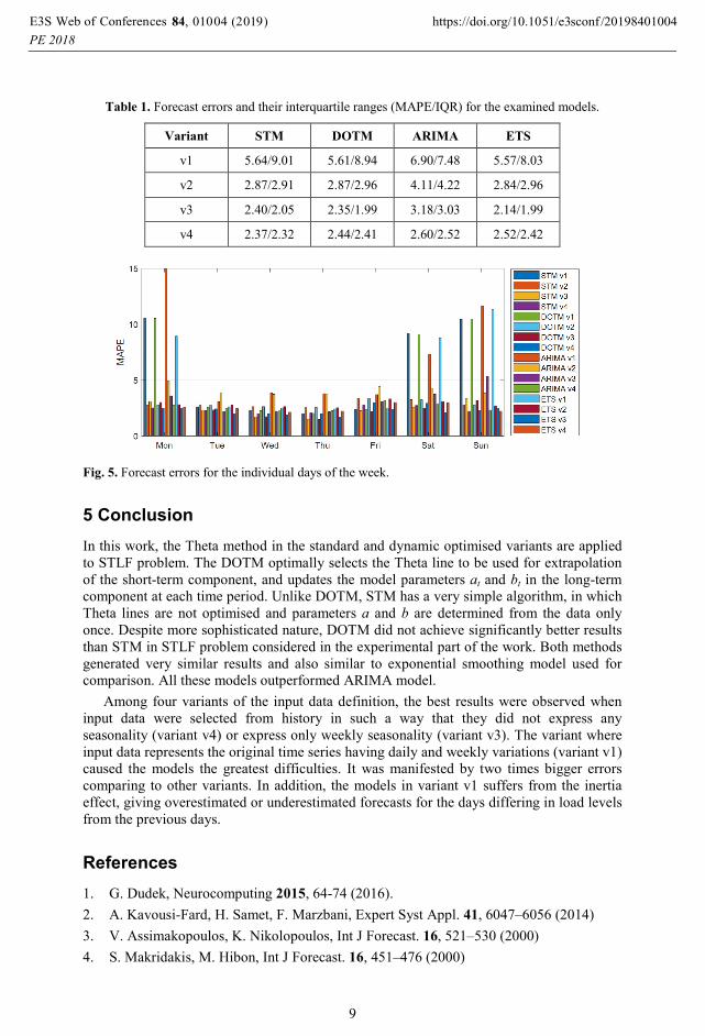
Table 1. Forecast errors and their interquartile ranges (MAPE/IQR) for the examined models.

Variant STM DOTM ARIMA ETS

v1 5.64/9.01 5.61/8.94 6.90/7.48 5.57/8.03

v2 2.87/2.91 2.87/2.96 4.11/4.22 2.84/2.96

v3 2.40/2.05 2.35/1.99 3.18/3.03 2.14/1.99

v4 2.37/2.32 2.44/2.41 2.60/2.52 2.52/2.42

Fig. 5. Forecast errors for the individual days of the week.

5 Conclusion

In this work, the Theta method in the standard and dynamic optimised variants are applied

to STLF problem. The DOTM optimally selects the Theta line to be used for extrapolation

of the short-term component, and updates the model parameters at and bt in the long-term

component at each time period. Unlike DOTM, STM has a very simple algorithm, in which

Theta lines are not optimised and parameters a and b are determined from the data only

once. Despite more sophisticated nature, DOTM did not achieve significantly better results

than STM in STLF problem considered in the experimental part of the work. Both methods

generated very similar results and also similar to exponential smoothing model used for

comparison. All these models outperformed ARIMA model.

Among four variants of the input data definition, the best results were observed when

input data were selected from history in such a way that they did not express any

seasonality (variant v4) or express only weekly seasonality (variant v3). The variant where

input data represents the original time series having daily and weekly variations (variant v1)

caused the models the greatest difficulties. It was manifested by two times bigger errors

comparing to other variants. In addition, the models in variant v1 suffers from the inertia

effect, giving overestimated or underestimated forecasts for the days differing in load levels

from the previous days.

References

1. G. Dudek, Neurocomputing 2015, 64-74 (2016).

2. A. Kavousi-Fard, H. Samet, F. Marzbani, Expert Syst Appl. 41, 6047–6056 (2014)

3. V. Assimakopoulos, K. Nikolopoulos, Int J Forecast. 16, 521–530 (2000)

4. S. Makridakis, M. Hibon, Int J Forecast. 16, 451–476 (2000)


PE 20184 (

9

5. D. Thomakos, K. Nikolopoulos, J. Forecast. 34, 220–229 (2015)

6. E. Spiliotis, V. Assimakopoulos, K. Nikolopoulos, Int J Prod Econ. (in press)

7. D. Thomakos, K. Nikolopoulos, IMA J. Manage. Math. 25 (1), 105–124 (2014)

8. C. Constantinidou, K. Nikolopoulos, N. Bougioukos, E. Tsiafa, F. Petropoulos, V.

Assimakopoulos, In: Ming, M. (Ed.), Information Engineering, Lect Note Inform Tech

25, 116–120 (2012)

9. J.A. Fioruci, T.R. Pellegrini, F. Louzada, F. Petropoulos, A.B. Koehler, Int. J. Forecast.

32 (4), 1151–1161 (2016.)

10. R.J. Hyndman, B. Billah, Int J Forecast. 19, 287-290 (2003)


PE 20184 (

10

short-term load forecasting using theta method

Documents