electric utility interest in solar energy systems
TRANSCRIPT

Electric Utility Interest in Solar Energy Systems
by
Jason A. Trzesniewski
A thesis submitted in partial fulfillment
of the requirements for the degree of
MASTER OF SCIENCE
(Mechanical Engineering)
at the
UNIVERSITY OF WISCONSIN - MADISON
1995
vi
Table of Contents
Abstract i
Acknowledgments iv
Table of Contents vi
List of Figures ix
List of Tables xii
CHAPTER 1 Introduction 1
1.1 Motivation for Research 2
1.2 Literature Review 4
1.3 Thesis Objective 5
CHAPTER 2 Background 7
2.1 Solar Energy Systems 8
2.1.1 Solar Domestic Hot Water 8
2.1.2 Photovoltaics 10
2.2 Electric Utility Interest in Solar Energy Systems 12
CHAPTER 3 Solar Energy and Conventional System Models 14
3.1 Domestic Hot Water Systems 15
3.1.1 System Configurations 15
3.1.1.1 EDHW System Model 15
3.1.1.2 One Tank SDHW System Model 17
3.1.1.3 Two Tank SDHW System Model 20
3.1.1.4 Other System Configurations 22
3.1.2 Residential Water Draw Representation 23

vii
3.1.3 Critical Timestep Considerations 25
3.1.4 Integrating the Demand for Hourly Output 27
3.2 Photovoltaic System 28
3.3 Summary 31
CHAPTER 4 Marginal Plant Model 32
4.1 Capacity Adjustments 32
4.1.1 Forced Outage Adjusted Capacity 33
4.1.2 Forced and Scheduled Outage Adjusted Capacity 34
4.2 Least Cost Model 37
4.3 Analysis of Results 39
4.4 Summary 44
CHAPTER 5 Quantifying Utility Costs and Benefits 45
5.1 Assessing the Costs of a Solar DSM Implementation 45
5.2 Assessing Energy Reduction and Its Value 46
5.3 Assessing Emission Reduction and Its Value 49
5.4 Assessing Demand Reduction and Its Value 52
5.4.1 Peak Load Hour Method 53
5.4.2 Capacity Contribution Index Method 56
5.5 Assessing the Value of Other Benefits 60
5.6 Summary 62
CHAPTER 6 Economic Analysis 63
6.1 Present Worth of Life Cycle Savings 63
6.2 Levelized Life Cycle Savings 66
6.3 Rate of Return of an Option 67
6.4 Summary 68
CHAPTER 7 Case Study 70

viii
7.1 Solar Energy System Performance 71
7.2 Demand Method Comparison 74
7.3 Isolated System Versus Interconnected System Analysis 76
7.4 Utility Impact Results 78
7.5 Summary 84
CHAPTER 8 Conclusions and Recommendations 86
8.1 Conclusions 86
8.2 Recommendations 87
APPENDIX A Utility Load and Plant Data 89
APPENDIX B TRNSYS Simulations 100
APPENDIX C FORTRAN Programs 149
BIBLIOGRAPHY 175
EUSESIA User’s Manual

1
CHAPTER 1 Introduction
Electric utilities can realize economic and environmental benefits from a large
scale implementation of solar energy systems. Reductions in energy use achieved with
solar domestic hot water (SDHW) systems and energy generation from photovoltaic (PV)
systems at the consumer level result in reductions in energy, emissions and demand at the
generation level, and improvements in system reliability through capacity contribution.
Additional utility benefits can be found in delaying power plant construction, electric
customer retention and government incentives such as tax credits given for equipment
investment and energy subsidies.
These benefits can be quantified in terms of dollars to give a utility an assessment
of the value that a large scale implementation of solar energy systems may have. Starting
in the late 1980’s the Sacramento Municipal Utility District (SMUD) offered customers
rebates on SDHW systems to encourage the use of solar energy. Not only did this
program offer a rebate off the total cost of the SDHW system, but it spread the balance
out in payments over ten years. Recently, Wisconsin Public Service (WPS) began a
program in which customers could lease a $2000 SDHW system for $140 down and $12
per month.
It is important to show electric customers that such solar energy demand-side

2
management (DSM) programs have value to them. Historically, homeowners have
tended to shy away from SDHW systems due to high first costs, perceived unreliability of
the systems and payback periods on the order of ten or more years. Such programs as
offered by SMUD and WPS help ease the burden of payment by the customer for solar
energy systems. Moreover, annual electric bill savings outweigh the annual payments for
the system, thus making SDHW attractive to consumers.
1.1 Motivation for Research
For a utility to consider solar DSM programs such as those offered by SMUD and
WPS, the programs must be beneficial to the utility. Central Vermont Public Service
Corporation attempted to assess system performance by an on-site monitoring of ten
SDHW test systems (Sinos, Lind and Kirby, 1995). This type of small scale monitoring
shows the consumer what their energy savings are, but shows insignificant impact at the
utility level. Utilities must look at a larger number of systems to assess the benefits that
solar energy systems can have.
Most utility analyses of solar energy systems stop at an assessment of energy
reduction. These assessments are usually based f-chart predictions (Duffie and Beckman,
1991) of monthly performance and are based on average temperature and radiation values
for the given month. This method predicts aggregate energy reduction reasonably well,
but it does not identify emission and demand reductions.
Utility analyses that attempt to address the demand reduction achieved by solar
options tend to look at the system performance on a single peak day or a group of peak
hours. This method fails to account for capacity contribution through demand reductions

Introduction 3
at all hours (Harsevoort and Arny, 1994). An hourly study of these capacity
contributions is needed to accurately assess the improvements in system reliability.
Furthermore, operating costs and emission characteristics are dependent on the last plant
to be added to the generation mix, known as the marginal plant. Operating costs and
emission characteristics are therefore time dependent as the marginal plant varies with
time.
An accurate analysis of the impact of solar energy systems must be an annual
assessment performed on an hourly basis. System performance is calculated using hourly
weather data for the city in which the utility’s customers are located. The marginal plant
for a given utility or group of utilities is calculated hourly with utility or region load
information and plant capacity data for each plant in the regional mix. With hourly
predictions of both system performance and the marginal plant, an accurate assessment of
energy, emissions and demand reductions can be made.
It is of vital importance to the correctness of the analysis that weather data and the
load data represent the same year. Both the utility load and the performance of solar
energy systems are largely driven by weather and the interaction is often well matched.
For summer peaking utilities, the peak load is often found on the hottest day of the year
that is accompanied with high levels of solar insolation. Winter peaking utilities in areas
where homes are heated by electric means tend to find peak loads on the coldest day of
the year. In northern climates, these peak load days are often clear days with high solar
insolation which follow clear nights. With these peak load observations, the weather-
load interaction is seen and the importance of using weather and load data from the same
year in an analysis becomes apparent.
A large number of systems must be considered for the analysis to have a

4 Introduction
significant impact on an electric utility. When considering photovoltaic systems as grid-
connected electric generators, the performance of many systems as seen by a utility at the
generation level can be reasonably assessed by simulating a single system as an average
system and scaling up the results. However, this method is not accurate when simulating
a large number of SDHW systems.
The impact of a large scale implementation of SDHW systems cannot be
estimated by one test site system. SDHW systems will not act identical to one another
due to storage and control differences and, most importantly, differences in water draw
profiles at individual locations. To assess the impact of many SDHW systems with one
simulation an appropriate average water draw must be used. This average water draw
can then be used in a simulation to predict the amount of energy required to heat the
mains temperature to a set point temperature and ultimately to predict the amount of
energy required at the electric utility generation level. With an appropriate average water
draw, a single average SDHW simulation may be used in conjunction with the energy
rate control (ERC) simulation method to predict the impact of many SDHW systems
(Cragan, 1994).
1.2 Literature Review
Grater (1992) showed that annual energy consumption of a single solar domestic
hot water system was less than that of an electric domestic hot water (EDHW) system,
but peak demand was the same in both cases. Grater then simulated multiple EDHW and
SDHW systems using random hot water draw profiles for each pair of simulations.
Through these multiple simulations Grater showed that not only was the SDHW energy
consumption less than that of the EDHW systems but, also, the SDWH systems showed

Introduction 5
lower peak demand. Grater concluded that a sample size of 400 systems is adequate to
predict a large scale impact of SDHW systems. The problem with Grater’s analysis was
the use of extreme and unlikely water draw profiles in some cases.
Warren (1993) addressed the issue of sample size in a study of gas furnaces.
Warren showed that a sample size of 100 systems provides adequate confidence in
determining the average demand of an ensemble of systems as compared to the average
demand of measured data. Warren then explored a single energy rate control (ERC)
using average system parameters as an alternative to a large number of temperature level
control (TLC) simulations. Warren found the ERC simulation to closely reflect the
average of greater than 1000 TLC simulations.
Cragan (1994) combined the ideas of energy rate control and an average hot water
draw profile to assess the impact on a utility of an ensemble of SDHW systems. Cragan
developed average weekday and weekend hot water draws using WATSIM, a program
that predicts typical household hot water draws, developed by the Electric Power
Research Institute (EPRI). Cragan showed that the use of an average water draw resulted
in a good estimate of average system performance. Cragan analysis employed the energy
rate control to simulate the demands required by SDHW and EDHW systems to supply
the hot water required by the developed water draws. The results were compared to
assess energy, emission and demand reductions at the generation level provided by the
ensemble of SDHW systems.
1.3 Objective of Research
The lack of a standard planning model that evaluates the benefits and costs of

6 Introduction
renewable technology is a significant barrier to utility integration of these technologies
(Wan and Parsons, 1993). This research aims to develop a standard methodology to
assess the benefits and costs of solar domestic hot water and photovoltaic systems to
utilities and electric customers. Advantages and disadvantages of a solar DSM program
are identified.
The objective is extended to automate the methodology into a software package to
be distributed to utilities so that any given utility can assess the benefits found in solar
energy systems. Innovative use of TRNSYS (Klein et al., 1994), a software package
developed by the University of Wisconsin-Madison Solar Energy Laboratory, and
TRNSED (Fiksel et al, 1994), an editing environment to TRNSYS, allow users to select
and and tailor solar energy systems to be used in the analysis. Users have the opportunity
to provide specific utility information that will affect the economic assessments.
TRNSYS is used to simulate conventional and solar energy system performance.
Subroutines added to the TRNSYS program allow for calculation of the marginal plant at
each hour of the year and the economics of a given option. Given system performance,
marginal plant data and user specified information, reductions in demand at the consumer
level are translated to reductions in energy, emissions and demand at the generation level
and quantified in terms of dollars. These savings are then combined with other identified
benefits to report the life cycle savings of a solar energy option.

7
CHAPTER 2 Background
A utility load is largely driven by weather that is often well matched with the
operation of solar energy systems. Most utilities tend to find peak loads in the summer.
These peak loads are largely driven by air conditioning demands and are on hot days with
high levels of solar insolation. These conditions are ideal for solar energy system
operation. With a sufficient number of solar energy systems on the demand side, a utility
can achieve a significant demand reduction.
Some winter peaking utilities can also realize demand benefits from solar energy
systems. Utilities that peak in the winter tend to be in areas where homes are generally
heated electrically. Peak loads are often found on the coldest day of the year when
heating demands are highest. In northern climates, the peak loads tend to be on clear
days following clear nights. These clear days allow for significant solar insolation that
promote solar energy system performance.
Summer and winter peaking utilities can both benefit from the energy and
emission reductions at the generation level. A large scale implementation of solar energy
systems can provide for significant annual reductions in energy use at the consumer level
resulting in annual energy and emission savings at the generation level. These benefits
along with the demand benefits can make solar energy systems an attractive demand-side

8
management option.
2.1 Solar Energy Systems
Two types of sola r energy systems are often considered for home use:
photovoltaics and solar domestic hot water. Photovoltaic systems convert solar radiation
to electricity. These systems can be connected to the grid to act as a small power plant.
Solar thermal systems use solar insolation to heat a medium such as air or water. SDHW
systems are a type of solar thermal system and are can be considered as a small power
plant in the sense that they reduce electric demand.
2.1.1 Solar Domestic Hot Water
Solar domestic hot water systems are used to preheat water that is to supply a hot
water load. The primary elements in an SDHW system are a solar collector, an auxiliary
tank with an auxiliary heating element, a pump and a controller. Other common
components include a heat exchanger and and a solar storage tank. Figure 2.1.1-1 depicts
a typical two-tank solar energy system.

Background 9
To Load
Tempering Valve
4.5 kW
Water Supply From Mains
Pump Controller
Pump
Collector
Solar Storage
Tank
Auxiliary Tank and Heating Element
HX
Figure 2.1.1-1: A Typical SDHW System
In this system the auxiliary heat input is a typical 4.5 kW electric heating element.
The heating element makes up for the energy not provided by the solar system to meet
the set point temperature of the water to be delivered to the load. The pump controller
monitors the temperatures at the bottom of the solar storage tank and at the outlet on the
collector plate. When the plate temperature reaches a temperature above that of the
bottom of the tank, the pump turns on, collecting useful thermal energy.
At times the system will collect sufficient energy so that no auxiliary heat input is
required. In summer it is not uncommon to find the temperature of the solar heated water
to exceed the set point temperature. In this case the water is tempered via the tempering
valve as shown in figure 2.1.1-1. The result is that the water draw out of the auxiliary
tank is less than that delivered to the load.
The heat exchanger is a common feature in cold climates used for freeze
protection. Without a heat exchanger the water from the storage tank is pumped through
the collector. Under freezing conditions, water in the lines can freeze causing damage to
the system. Ethylene glycol-water and propylene glycol-water solutions are the most
common anti- freeze heat exchanger fluids used in SDHW applications. Another form of

10 Background
freeze protection is known as drain-back. In a drain-back system, the water that would
remain in the lines is drained into the tank or a sump to keep it from freezing (Duffie and
Beckman, 1991).
2.1.2 Photovoltaics
Photovoltaic systems are used to convert solar energy into electrical energy. The
primary components of a grid-connected photovoltaic system include a photovoltaic
panel, a maximum power point tracker and a DC/AC converter. The photovoltaic panel
is made up of may individual photovoltaic cells connected in series. Figure 2.1.2-1
illustrates a typical grid-connected photovoltaic system.
Solar Panel
DC/AC Converter
DC/DC Maximum
Power Point Tracker
Figure 2.1.2-1: A Typical Grid-Connected Photovoltaic System
The rudimentary physics behind the photovoltaic process is that an atom or
molecule of the material that makes up the cell absorbs a photon of the solar radiation. If
the energy level of the photon is high enough, the absorption of the photon frees an
electron from the atom or molecule. This process of freeing electrons ultimately results
in the electricity produced by a PV cell. Common materials used in photovoltaic cells are
silicon, cadmium sulfide and gallium arsenide (Duffie and Beckman, 1991).
The current and voltage characteristics of a photovoltaic cell changes as the leve l
of incident radiation changes. Figure 2.1.2-2 displays the trends of the I-V curves for a

Background 11
typical photovoltaic cell for changes in radiation level and is intended for illustration
purposes only. Figure 2.1.2-2 shows that as the incident radiation level increases higher
currents can be achieved. Many operation points are possible for a given radiation level.
However, it is most desirable to operate at the maximum power point for a given incident
radiation level, marked by an ‘X’ in figure 2.1.2-2.
Cur
rent
[A
mps
]
Voltage [Volts]
Increasing Radiation Level
Maximum Power Point
Figure 2.1.2-2: I-V Curve for a Typical PV Cell
The DC current drawn from the photovoltaic cell is fed to a DC/DC maximum
power point tracker. The maximum power tracker varies resistance to maintain a near
optimum operating condition. In most cases the maximum power tracker also converts
the power to correspond to the voltage that is required by the load. The resulting voltage-
corrected power is fed through a DC/AC converter where the DC current is converted to
an AC current with a frequency and voltage matching that of the grid.
2.2 Electric Utility Interest in Solar Energy Systems
Utilities considering a solar DSM program must identify the potential benefits and
costs of the option. Costs related to such a program include the initial investment
required to purchase the systems, administrative costs and any operation and maintenance

12 Background
costs that may be associated with the systems. Generally there is no operation costs to
the utility associated with solar energy systems as the customers pay for the energy
required to run the systems.
Solar energy systems offer benefits such as reductions in energy, emissions and
demand. Reductions in energy achieved by SDHW systems and the energy generated by
PV systems at the customer level directly result in these benefits at the generation level.
Other benefits may be found in government incentives offered to promote renewable
energies. These incentives include tax credits given towards the investment in renewable
energy and a subsidy given for energy production by the system.
It is up to the utility to place other values on the program. For example, a utility
may include customer retention as a benefit of a solar DSM program. It is possible that
an electric utility may lose electric customers to an alternate fuel such as natural gas for
water heating. With a solar energy program, a utility may retain a portion of these
customers that would otherwise be lost. Additionally, solar energy programs may bring
in new customers, capturing a larger market. Utilities that deal in both electricity and gas
may want to consider customer retention as a benefit as a higher profit margin is often
realized on electricity than on natural gas.
Utilities may also consider placing value on delayed power plant construction.
Solar energy systems effectively add capacity to a utility’s generation mix. The effective
capacity added by solar energy systems may be significant enough to delay the
construction of new facilities. This can be viewed as taking further credit for peak
demand reduction. Once the potential benefits of a solar DSM option are identified, they
can be quantified.

14
CHAPTER 3 Solar Energy and Conventional System Models
To evaluate the impact of a large scale implementation of solar energy systems on
an electric utility, knowledge of solar system performance is needed. This chapter
develops the system models used to simulate a large number of solar energy systems.
The intent is to represent the results of a large number of simulations with a single
simulation. From the solar system models, the system performance can be predicted. The
system performance is used to evaluate energy, emission and demand reductions at the
generation level.
The transient system simulation program TRNSYS (Klein et al., 1994) developed
by the University of Wisconsin Solar Energy Lab is used to simulate solar energy system
performance. TRNSYS is a modular program that contains subroutines known as
TYPES that represent the components found in solar energy systems among others. By
correctly specifying the time dependent inputs and fixed parameters that define each
TYPE, the solar energy systems are simulated.
Certain parameters of the solar energy and conventional system models can be
edited through TRNSED (Fiksel et al., 1994). The sections describing the system models
are concluded with a discussion of the parameters that can be edited. Default values are
given as typical system parameters.
3.1 Domestic Hot Water Systems

15
Average system demands of both SDHW and EDHW systems are found in order to evaluate the
impact that a large scale implementation of SDHW systems has on an electric utility. Utilities realize
reductions in energy, emissions and demand due to the performance of an ensemble of SDHW systems. A
representative EDHW system is needed as a comparative system to judge SDHW system performance
against. An average residential water draw is obtained to predict the average amount of energy required by
the SDHW and EDHW systems.
3.1.1 System Configurations
Typical EDHW and SDHW models are developed using TRNSYS. One and two
tank SDHW systems are modeled to assess their performances compared to an EDHW
system. Certain system parameters are made visible through the TRNSED front-end.
Representing one and two tank models through TRNSED allows for a wide variety of
systems to be simulated as system parameters can be changed.
3.1.1.1 Electric DHW System Model
The EDHW system model is depicted in figure 3.1.1.1-1. The system consists of
a electric hot water storage tank with two 4.5 kW heating elements. The tank supplies a
residential hot water load. Water from the mains replaces the water drawn from the tank
to supply the load. To simulate stratification, the storage tank is modeled as a three node
tank, representing three temperature levels within the tank. A heating element is located
in both the top and bottom third of the tank. The heating elements are controlled on a
master/slave relationship. With this control, only one element may be on at a given time
so that the maximum power demand is 4.5 kW. This arrangement is typical of standard
EDHW systems.

4.5 kW Heating Elements
Electr ic Tank
To L oad
From Water Mains
Figure 3.1.1.1-1: The EDHW System Model
The EDHW system supplies hot water at a given set point temperature. The set
point temperature used in the EDHW model is 140¡ F (60¡ C). The set point
temperature is a fixed system parameter. The heating element supplies electric power to
maintain the upper third of the tank at the set point temperature.
System parameters can be changed through the TRNSED front-end. The tank
parameters available in the TRNSED front-end are the volume and height, and the
insulation R value. The magnitude of the average daily water draw can also be changed
(see section 3.1.2). These parameters are made available so that a system can best be
represented for a given location. Table 3.1.1.1-1 summarizes default parameters typical
to an EDHW system. The tank parameters are taken from the SRCC ratings (SRCC,
1994).
8/6/2002Table 3.1.1.1-1: Typical EDHW System Parameters
Tank Parameters
Tank Volume 80 [gallons] Tank Height
4.89 [ft] Insulation R Value 16.7 [hr-ft2-F/Btu]
Water Draw Parameters
Average Daily Water Draw 69 [gallons/day]

Solar Energy and Conventional System Models 17
17
3.1.1.2 One Tank SDHW System Model
The one tank SDHW system model is depicted in figure 3.1.1.2-1. The system
consists of a collector, auxiliary tank with a 4.5 kW heating element, pump and
controller. The heating element in the auxiliary tank provides heat input that is not
provided by the solar collector to maintain the upper third of the tank at the set point
temperature of 140¡ F. The bottom heating element of the tank is disabled, leaving only
the top element. The controller initiates flow through the collector by monitoring the
temperatures at the bottom of the tank and at the collector outlet.
4.5 kW
Auxiliary Tank and Heating Element
To Load
From Water Mains
Tempering Valve
Collector
Pump
Controller Figure 3.1.1.2-1: The One Tank SDHW System Model
A tempering valve is introduced to the system in case the tank temperature is
above the set point temperature. If the tank temperature is above the set point, the
tempering valve mixes mains water with the water from the tank, thus reducing the draw
from the tank. The new tank draw can be found with mass and energy balances on the
tempering valve, assuming a constant specific heat of water. Equation 3.1.1.2.1 gives the

water draw from the tank when the tank temperature is above the set point temperature.
mass balance:
mtank + mmains = mload
energy balance:
mtank cpTtank + mmains cpTmains = mloadcpTset point
Rearranging and substituting for mmains :
mtank = mload
Tset point - TmainsTtank - Tmains (3.1.1.2.1)
System parameters can be changed in the TRNSED front-end. The tank
parameters and magnitude of the water draw can be specified, as in the case of the
EDHW system (see section 3.1.1.1), as well as the solar collector parameters. Solar
collector parameters accessible through the TRNSED front-end include the number of
collectors that make up the system, collector area, slope, FR(τα) and FRUL. A heat
exchanger, as depicted in figure 2.1.1-1, can also be added to the system through
TRNSED. The heat exchanger parameters that can be modified are the heat exchanger
effectiveness and the specific heat of the collector side fluid. A typical heat exchanger
effectiveness is 0.5 or less. The specific heat of ethylene glycol, a typical collector side
fluid used with a heat exchanger is 0.577 Btu/lbm-F. If no heat exchanger is desired, the
effectiveness is entered as -1. The pump size is specified by entering the power
consumption of the pump in Watts. Table 3.1.1.2-1 summarizes default parameters
typical to a one tank SDHW system. Collector parameters are typical to an SRCC rated
collector.
8/6/2002Table 3.1.1.2-1: Typical One Tank SDHW System Parameters
Tank Parameters
Tank Volume 80 [gallons]
Solar Energy and Conventional System Models 19
Tank Height 4.89 [ft] Insulation R Value 16.7 [hr-ft2-F/Btu] Solar Collector Parameters
Number of Collectors in Array
Area 60 [ft2]
R(τα)
.70 RUL
.749 [Btu/hr- ft2-F] Slope 23 [degrees] Heat Exchanger Parameters
Effectiveness
Specific Heat of Collector Side Fluid 0.0 [Btu/lbm-F] Pump Parameters
Pumping power 50 [W] Water Draw Parameters
Average Daily Water Draw 69 [gallons/day]
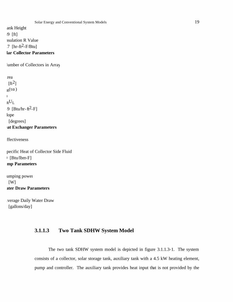
3.1.1.3 Two Tank SDHW System Model
The two tank SDHW system model is depicted in figure 3.1.1.3-1. The system
consists of a collector, solar storage tank, auxiliary tank with a 4.5 kW heating element,
pump and controller. The auxiliary tank provides heat input that is not provided by the

collector to supply the load at the set point temperature of 140¡ F. The bottom heating
element of the tank is disabled, leaving only the top element. The controller initiates
flow through the collector by monitoring the temperatures at the bottom of the tank and at
the collector outlet. The tempering valve operates in the same manner as described in the
one tank SDHW model.
To Load
From Water Mains
Tempering Valve
Collector
Pump
Controller
4.5 kW
Auxiliary Tank and Heating Element
Solar Storage
Tank
Figure 3.1.1.3-1: The Two Tank SDHW System Model
System parameters can be changed through the TRNSED front-end. The
parameters that can be altered are the same as in the one tank SDHW model with the
addition of the solar storage tank parameters. A heat exchanger can be added between
the collector and solar storage tank as described in the one tank model. Table 3.1.1.3-1
summarizes default parameters typical to a two tank SDHW system simulation.
8/6/2002Table 3.1.1.3-1: Typical Two Tank SDHW System Parameters
Auxiliary Tank Parameters
Tank Volume 80 [gallons]
ank Height 4.89 [ft] Insulation R Value 16.7 [hr-ft2-F/Btu] Solar Storage Tank Parameters
Solar Energy and Conventional System Models 21
Tank Volume 80 [gallons] Tank Height 4.89 [ft] Insulation R Value 16.7 [hr-ft2-F/Btu] Solar Collector Parameters
Number of Collectors in Array
Area 60 [ft2]
R(τα)
.70 RUL
.749 [Btu/hr- ft2-F] Slope 23 [degrees] Heat Exchanger Parameters
Effectiveness
Specific Heat of Collector Side Fluid 0.0 [Btu/lbm-F] Pump Parameters
Pumping power 50 [W] Water Draw Parameters
Average Daily Water Draw 69 [gallons/day]
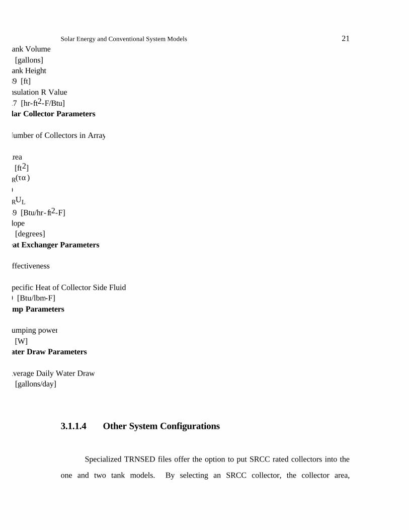
3.1.1.4 Other System Configurations
Specialized TRNSED files offer the option to put SRCC rated collectors into the
one and two tank models. By selecting an SRCC collector, the collector area,
FR(τα), FRUL and incidence angle modifiers are fixed in the simulation (SRCC, 1994).
Use of SRCC rated collector parameters allows for assessing system performance using
parameters of real solar collectors.
Other SDHW system configurations, such as photovoltaic pumps and
thermosyphons, can be modeled with TRNSYS. With knowledge of TRNSYS, specific
systems that are to be considered as solar DSM options can be simulated to assess system
performance. Section 5.6 of the EUSESIA User’s Manual (Trzesniewski et al., 1995) in
Appendix A describes the considerations involved in modeling a system.
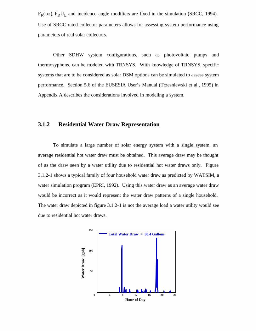
3.1.2 Residential Water Draw Representation
To simulate a large number of solar energy system with a single system, an
average residential hot water draw must be obtained. This average draw may be thought
of as the draw seen by a water utility due to residential hot water draws only. Figure
3.1.2-1 shows a typical family of four household water draw as predicted by WATSIM, a
water simulation program (EPRI, 1992). Using this water draw as an average water draw
would be incorrect as it would represent the water draw patterns of a single household.
The water draw depicted in figure 3.1.2-1 is not the average load a water utility would see
due to residential hot water draws.
50
100
150
0 4 8 12 16 20 24
Wat
er D
raw
[gp
h]
Hour of Day
Total Water Draw = 58.4 Gallons

Solar Energy and Conventional System Models 23
Figure 3.1.2-1: A Typical Household Daily Hot Water Draw (Cragan, 1994)
Cragan (1994) addressed the issue of finding an average water draw profile
representative of residential hot water draws. Employing WATSIM, nine hundred
separate household water draws, as the one shown in figure 3.1.2-1, were simulated. The
resulting nine hundred profiles were averaged and smoothed to find average weekday and
weekend water draw profiles. Figure 3.1.2-2 shows the resulting hot water draws that are
used in the EDHW and SDHW system simulations. These draws result in an aggregate
draw of approximately 69 gallons/day.
0
2
4
6
8
0 6 12 18 24
Daily Water Draw = 69 gallons
Weekend [gal/hr]Weekday [gal/hr]
Ave
rage
Wat
er D
raw
[ga
l/hr]
time [hr]
Figure 3.1.2-2: Average Weekday and Weekend Hot Water Draw Profiles
The water draw used in the domestic hot water systems can be scaled through the
TRNSED front-end. The front-end offers an opportunity to specify the average daily
water draw for a location. To scale the draw, the hourly value is multiplied by the value
input in TRNSED and divided by the basis (69 gallons/day).

3.1.3 Critical Timestep Considerations
When simulating a domestic hot water system, care must be taken in defining the
simulation timestep. A model that is simulated at a timestep greater than the critical
timestep can go unstable. When simulating domestic hot water systems, the critical
timestep can be reduced to a function of the volume of the tank (Vtank), the number of
tank nodes (N) and the volumetric flow rates of any flow into and out of the tank. The
flows through the tank are the flow due to the water draw (Vdraw) and the flow to the
collector (Vcollector) Equation 3.1.3.1 gives an expression for the critical timestep.
∆tcritical = Vtank
N Vdraw + Vcollector 3.1.3.1
In this simulation the tank size and magnitude of the water draws are parameters
that can be changed in the TRNSED front-end. To correctly assign the critical timestep
an extreme case is identified which yields the smallest critical timestep. Referring to
equation 3.1.3.1 it can be seen that the critical timestep will be smallest when the tank
volume is small and the draw from the tank is large. Two assumptions must be made to
define the extreme case. First, it is assumed that the smallest tank size that will be
simulated is a 40 gallon tank. Second, it will be assumed that the maximum flow rate to
the load will be 10 gallons/hr. Referring to figure 3.1.2-2 it can be seen that a for a daily
water draw of 69 gallons/day, the maximum draw is around 23 kg/hr (6 gallons/hr).
Realistically, an average daily draw for an area would not be more than 100 gallons/day,
which results in a maximum draw of around 9 gallons/hr. A maximum draw of 10
gallons per hour is chosen to add a safety factor into the critical timestep calculation.
The flow rate through the collector side of the tank is fixed at 86 gallons/hr (325
kg/hr) and the tank is modeled with three nodes. Using this fixed information along with
the two assumptions previously discussed, the critical timestep can be found from
equation 3.1.3.1. This evaluation results in a critical timestep of 0.139 hr. The critical

Solar Energy and Conventional System Models 25
timestep chosen for the simulations is 0.1 hr, slightly less than the critical timestep.
Table 3.1.3-1 summarizes the parameters used in determining the simulation timestep.
8/6/2002Table 3.1.3-1: Parameters Used in Timestep Consideration
Minimum Tank Volume 40 [gallons] Number of Tank Nodes 3 (fixed) Collector-Side Flow 86 [gph] (fixed) Maximum Tank Draw 10 [gph] Critical Timestep 0.139 [hr] Simulation Timestep 0.1 [hr]
25
3.1.4 Integrating the Demand for Hourly Output
The assessment of the impact of large scale implementation of solar energy
systems is performed on an hourly basis. Thus, the system performance must be reported
on an hourly basis. However, in order to meet critical timestep criteria, the simulation is
run at a tenth of an hour timestep. To output the demand requirement of a DHW system
on an hourly basis, the demand requirements at each timestep must be integrated over the
hour in which they occur. This integration is done by sending the demand requirements
of a system through the TRNSYS TYPE 24 integrator which is reset hourly. Table
3.1.4.-1 lists the hourly demand output from the DHW system models.
8/6/2002Table 3.1.4-1: EDHW and SDHW System Hourly Model Outputs
EDHW Model aux
SDHW Model

aux + Ppump
A few words need to be said about assessing the heat input requirements of the system. Cragan (1994) used the energy rate control approach (ERC) where an just enough heat was input into the water draw of the load to instantaneously raise it to the set point temperature. In this approach the heating element is assumed to have an infinite heat rate and tank losses are modeled as only from the top third of the tank which is assumed to be at the set point temperature. The required heat input is integrated over the hour.
The energy rate control approach is also used in the DHW models previously discussed, although it is not as apparent. The nature of the tank models in TRNSYS is essentially that of ERC except that the rate of input is limited to 4.5 kW rather than an infinite rate. As long as the integrated required heat input does not exceed 4.5 kW, the heating element in the tank acts as an ERC zip heater. This approach is somewhat more accurate than the method used by Cragan since the tank losses are not assumed, as in Cragan’s work, and are correctly accounted for.
3.2 Photovoltaic Systems
To assess the performance of a PV system a model is developed to output the
hourly electric generation of the system. Since the PV system generates electricity rather
than reduces electricity consumption, no comparative system is needed in the analysis.
Electricity produced by the PV system at the customer level is reflected in energy,
emission, and demand reductions at the generation level.
Figure 3.2-1 depicts the PV system model used for simulation. The system
consists of a photovoltaic array, a maximum power point tracker and a DC/AC converter.
Electricity produced by the cell is fed to the maximum power point tracker which
maximizes the power by selecting the appropriate operating voltage and current. The DC
signal is then converted to an AC current and the signal is adjusted to the grid voltage and
frequency through the DC/AC converter.
Solar Panel
DC/DC Maximum
Power Point Tracker
DC/AC Converter
To Grid

Solar Energy and Conventional System Models 27
Figure 3.2-1: The PV System Model
A PV panel has parameters that are characteristic to its manufacturing and
reference conditions. Parameters that define the I-V curve at reference irradiation and
temperature conditions include the open circuit voltage (Voc) and short circuit current
(Isc) and maximum power voltage (VPmax) and maximum power current (IPmax) as
depicted in figure 3.2-2. The open and short circuit temperature coefficients (µV,oc and
µI,sc) are defined as the change in open circuit voltage and short circuit current with
respect to temperature (dVoc/dT and dIsc/dT) respectively (Duffie and Beckman, 1991).
Other parameters characteristic to the manufacturing of the panel include the
transmittance-absorptance product (τα), material band gap, number of individual cells in
series per panel, panel width and panel length.
Cur
rent
[A
mps
]
Voltage [Volts]
VocVPmax
IPmax
IscMaximum Power Point
Figure 3.2-2: The I-V Curve at Reference Conditions
In the PV model these parameters are fixed through selection of specific
manufactured panels. Table 3.2-1 summarizes the characteristic parameters of two such
panels, the Advanced Photovoltaic Systems Inc. model EP-50 and the Solarmodule
model AEG PQ.
8/6/2002Table 3.2-1: PV Panel Parameters
Manufacturer and Model

Advanced Photovoltaic Systems Inc. EP-50 Solarmodule AEG PQ Reference Irradiation 1000 [W/m2] 1000 [W/m2] Ref. Cell Temperature 298 [K] 298 [K]
at Reference
1.8 [Amps] 2.41 [Amps]
oc at Reference
55.5 [Volts] 22.4 [Volts] Pmax at Reference
1.32 [Amps] 2.2 [Amps]
Pmax at Reference
38 [Volts] 17.45 [Volts]
I,sc
0.0015 0.0014954
V,oc
0.19425 0.090092 τα)
0.9 0.9 Material Band Gap 1.155 1.155 # Cells in Series per Panel
Panel Width 0.8 [m] 0.46 [m] Panel Length 1.525 [m] 1.076 [m]
28
The PV system can be changed in the TRNSED front-end. The number of

Solar Energy and Conventional System Models 29
collectors that make up the system and their slope can be specified through TRNSED.
Power is lost in both the maximum power point tracker and the DC/AC converter. The
efficiency of these two components can be specified through the front-end. The grid
operating voltage can also be specified in the TRNSED front-end. Table 3.2-2
summarizes default parameters typical to a PV system.
8/6/2002Table 3.2-2: Typical PV System Parameters
PV Panel System Parameters
Number of panels in series
Number of panels in parallel
Slope 23 [degrees] Maximum Power Point Tracker Parameters
Efficiency 0.95 DC/AC Converter Parameters
Efficiency 0.95 Grid Operating Voltage 110 [Volts]
29
3.3 Summary
Models for EDHW, SDHW and PV systems are developed in this chapter. DHW
system models must be simulated at timesteps below the critical timestep. An average
water draw is used in the DHW systems so that one simulation can represent the average
of a large number of simulations. The demand of an EDHW system is the amount of heat
input required to raise the water supply to the set point temperature. The demand of the

SDHW system is the amount of auxiliary heat input required to heat the solar preheated
water to the set point temperature plus the pumping power required move the water
through the collector. The PV system is controlled to generate electricity at the
maximum power point. The electricity generated is supplied to the grid at the grid
operating voltage. The models output hourly demands for the electric and solar DHW
systems and the hourly grid-connected generation of a PV system.

32
CHAPTER 4 Marginal Plant Prediction Model
The marginal plant at each hour of the year must be identified to correctly assess
the energy and emission savings to a utility. The value of energy saved by a demand-side
efficiency measure is based on the operating cost of the marginal plant. Similarly, the
avoided emissions are related to the emission characteristics of the marginal plant. A
model is developed to identify the marginal plant. The model is based on adding adjusted
plant capacities to the generation mix on a least cost basis to meet the load. Plant specific
data used in the example calculations are taken from Advance Plan 7, Technical Support
Document D24: Power Supply (Public Service Commission of Wisconsin, 1994).
4.1 Capacity Adjustments
Utility electric generating plants face forced and scheduled outages during their
operation. In order to predict the marginal plant, a methodology is set up to adjust the
capacity to account for these outages. The year is broken down into two general seasons,
a peak season and a maintenance season. For example, the maintenance seasons may be
defined as the spring and fall months when the load is relatively low. The peak seasons
then are the winter and summer months when utilities tend to find relatively higher
demands. During the peak season, the capacity is adjusted to account for forced outages
only. In the maintenance season, the plant capacity is adjusted to account for forced and
scheduled outages.

Marginal Plant Prediction Model 33
4.1.1 Forced Outage Adjusted Capacity
Electric generating plants may face full forced outages in which case the entire
capacity of the plant is lost, or partial forced outages where only a fraction of the capacity
is lost. The forced outage adjusted capacity considers both types of outages. Because the
exact time of a forced outage cannot be predicted, the forced outage adjusted capacity is
calculated statistically based on historical frequency of occurrence. The full forced
outage and up to four levels of partial forced outage are accounted for in the forced
outage adjusted capacity.
To adjust the nameplate capacity for forced outages, a forced outage adjustment
factor is first calculated (FOA factor). The FOA factor is calculated with forced outage
and capacity information. The FOA factor is defined in equation 4.1.1.1.
FOA factor= 1 - fullout - partout i*partcapi
Capacity•i = 1
4
(4.1.1.1)
In this equation, fullout and partout are historical fractions of time in which a
generating unit experiences full and partial outages respectively. The variable partcap is
the remaining capacity that is available for service in the case of a partial outage. It is not
the amount of capacity that is lost during the partial outage. The FOA factor is used with
the nameplate capacity of the plant to calculate the forced outage adjusted capacity (FOA
capacity ) as defined in equation 4.1.1.2.
FOA capacity = FOA factor * Capacity (4.1.1.2)
The FOA capacity is an effective capacity used to find the marginal plant during

times when the plant is assumed to be operating in the peak season. Table 4.1.1-1
summarizes the FOA capacity and the information required to calculate it for a given mix
of generating plants. The data are representative of Wisconsin Electric Power Company
in Milwaukee, WI. The FOA capacity is used for further calculation when adjusting the
capacity for scheduled outages.
4.1.2 Forced and Scheduled Outage Adjusted Capacity
In addition to adjusting plant capacity for forced outages, capacity also needs to
be adjusted for scheduled outages. At times a utility knows exactly when it will take a
plant off line. If this is the case, the scheduled outage information can be entered to make
the forced and scheduled outage capacity (FSOA capacity) zero. However, there are
times when a utility may know only a given time frame in which a plant will be off line.
If this is the case, the FSOA capacity has a value and the effective plant capacity is a
fraction of its nameplate capacity. This type of adjustment particularly makes sense
when looking at a region of utilities in which case it is hard to identify when neighboring
utilities will take their plants off line.

Marginal Plant Prediction Model 35
Table 4.1.1-1: WEPCO Forced Outage Adjusted Capacity InformationNameplate Capacity [MW]
Full OutageRate
[%]
Partial Outage Rate
[%]
Partial Capacity
[MW]
FOA Capacity [MW]
Point Beach 2 Point Beach 1 Oak Creek 8 Oak Creek 7 Oak Creek 6 Oak Creek 5 Port Washington 4 Port Washington 3 Port Washington 2 Port Washington 1 Valley 4 Valley 3 Valley 2 Valley 1 Pleasant Prair ie 2 Pleasant Prair ie 1 Presque I sle 9 Presque I sle 8 Presque I sle 7 Presque I sle 6 Presque I sle 5 Presque I sle 4 Presque I sle 3 Presque I sle 2 Presque I sle 1 Edgewater 5 Concord 4 Concord 3 Concord 2 Concord 1 Germantown 4 Germantown 3 Germantown 2 Germantown 1 Oak Creek 9 Point Beach 5 Port Washington 6
1.9 1.9
1 1 2 2 4 4 4 4
2.5 1
2.5 1 1 1 1 1 1 1 1 1 1 0 0 2 1 1 1 1 1 1 1 1 1 1 1
0 0
1.6 1.6
3 2.9 1.5 1.4 1.3 1.3
4 15 3.9 13 1.3 1.3
3 3
3.2 2.2 2.2 2.4 2.4
0 0 5 0 0 0 0 0 0 0 0 0 0 0
0 0
85 85 82 82 29 29 29 29 34 14 30
7 220 220
14 14 13 20 19 12 12
0 0
38 0 0 0 0 0 0 0 0 0 0 0
Generating Plant and Unit
497 497 305 280 260 258
80 82 80 80 70 70 62 64
580 580
84 83 81 85 84 57 58 37 25 97 83 83 83 83 53 53 53 53 20 20 18
5138
487.6 487.6 300.6 275.8 252.3 250.5 76.4 78.3 76.4 76.4 66.9 67.2 59.3 62.5
571.3 571.3 82.7 81.8 79.8 83.7 82.7 56.1 57.1 37.0 25.0 93.2 82.2 82.2 82.2 82.2 52.5 52.5 52.5 52.5 19.8 19.8 17.8
5035.5
To adjust the capacity to account for scheduled outages, scheduled outage
information is needed to calculate a scheduled outage adjustment factor (SOA factor).
The information required includes the scheduled outage, actual amount of time that a
plant is taken off line during the year, and the duration of the maintenance period.
Equation 4.1.2.1 defines the SOA factor.

SOA factor= 1 - scheduled outage
outage period (4.1.2.1)
The outage period is the range of time that the scheduled outage could occur in.
Note that by making the outage period equal to the scheduled outage the SOA factor goes
to zero. Thus, if a utility knows exactly when a plant is to be off line it can be reflected
with a forced and scheduled outage capacity of zero. Equation 4.1.2.2 shows the
calculation of the FSOA capacity.
FSOA capacity = SOA factor * FOA capacity (4.1.2.2)
Note that the FSOA capacity is based on the capacity previously adjusted for
forced outages. This adjustment is to account for the possibility of a forced outage during
the maintenance period. Table 4.1.2-1 summarizes the FSOA capacity and the
information required to calculate it for WEPCO. With the seasonal adjusted capacities
calculated, the marginal plant can be found.

Marginal Plant Prediction Model 37
Table 4.1.2-1: WEPCO Forced and Scheduled Outage Adjusted Capacity Information
Generating Plant and Unit
Scheduled Outage Periods
(month/day)
Outage Period [hrs]
Scheduled Outage [wks]
Point Beach 2 Point Beach 1 Oak Creek 8 Oak Creek 7 Oak Creek 6 Oak Creek 5 Port Washington 4 Port Washington 3 Port Washington 2 Port Washington 1 Valley 4 Valley 3 Valley 2 Valley 1 Pleasant Prairie 2 Pleasant Prairie 1 Presque Isle 9 Presque Isle 8 Presque Isle 7 Presque Isle 6 Presque Isle 5 Presque Isle 4 Presque Isle 3 Presque Isle 2 Presque Isle 1 Edgewater 5 Concord 4 Concord 3 Concord 2 Concord 1 Germantown 4 Germantown 3 Germantown 2 Germantown 1 Oak Creek 9 Point Beach 5 Port Washington 6
3/1 - 5/1 3/1 - 5/1 3/1 - 5/1 3/1 - 5/1 3/1 - 5/1 3/1 - 5/1 3/1 - 5/1 3/1 - 5/1 3/1 - 5/1 3/1 - 5/1 3/1 - 5/1 3/1 - 5/1 3/1 - 5/1 3/1 - 5/1 3/1 - 5/1 3/1 - 5/1 3/1 - 5/1 3/1 - 5/1 3/1 - 5/1 3/1 - 5/1 3/1 - 5/1 3/1 - 5/1 3/1 - 5/1 3/1 - 5/1 3/1 - 5/1 3/1 - 5/1 3/1 - 5/1 3/1 - 5/1 3/1 - 5/1 3/1 - 5/1 3/1 - 5/1 3/1 - 5/1 3/1 - 5/1 3/1 - 5/1 3/1 - 5/1 3/1 - 5/1 3/1 - 5/1
9/20 -11/20 9/20 -11/20 9/20 -11/20 9/20 -11/20 9/20 -11/20 9/20 -11/20 9/20 -11/20 9/20 -11/20 9/20 -11/20 9/20 -11/20 9/20 -11/20 9/20 -11/20 9/20 -11/20 9/20 -11/20 9/20 -11/20 9/20 -11/20 9/20 -11/20 9/20 -11/20 9/20 -11/20 9/20 -11/20 9/20 -11/20 9/20 -11/20 9/20 -11/20 9/20 -11/20 9/20 -11/20 9/20 -11/20 9/20 -11/20 9/20 -11/20 9/20 -11/20 9/20 -11/20 9/20 -11/20 9/20 -11/20 9/20 -11/20 9/20 -11/20 9/20 -11/20 9/20 -11/20 9/20 -11/20
2928 2928 2928 2928 2928 2928 2928 2928 2928 2928 2928 2928 2928 2928 2928 2928 2928 2928 2928 2928 2928 2928 2928 2928 2928 2928 2928 2928 2928 2928 2928 2928 2928 2928 2928 2928 2928
6 6 5 5 5 5 0 0 0 0 0 0 8 8 6 6 1 1 1 1 1 1 1 0 0 4 0 0 0 0 0 0 0 0 0 0 0
FSOA Capacity [MW]
1008 1008
840 840 840 840
0 0 0 0 0 0
1334 1334 1008 1008
168 168 168 168 168 168 168
0 0
672 0 0 0 0 0 0 0 0 0 0 0
Scheduled Outage
[hrs]
3889.9
319.7 319.7 214.4 196.7 179.9 178.6
76.4 78.3 76.4 76.4 66.9 67.2 32.3 34.0
374.6 374.6
78.0 77.1 75.2 78.9 78.0 52.9 53.9 37.0 25.0 71.8 82.2 82.2 82.2 82.2 52.5 52.5 52.5 52.5 19.8 19.8 17.8
4.2 Least Cost Model
The marginal plant is found on the premise that the plants are added to the
generating mix on a least cost basis. Utilities may have reason to employ plants on an
ulterior basis. For example, a plant that has poor emission characteristics may be kept

off- line in favor of a more expensive but cleaner plant. However, it is economically
beneficial for a utility to add plants to the mix on a least cost basis as operating costs are
minimized and higher profit margins are achieved. Although utilities may not
consistently add plants to the generating mix on a least cost basis, it is a generality and a
reasonable assumption.
Given the load at each hour of the year, the adjusted capacity of each plant is
added to the mix on a least cost basis until the load is met. If the hour of the year is
within the maintenance season for a given plant, the FSOA capacity is used as its
effective capacity to meet the load with. Otherwise, it is in the peak season and the FOA
capacity is used as the effective plant capacity for the hour. Table 4.2-1 summarizes the
least cost ordering of the plant mix along with the nameplate, FOA and FSOA capacities
for WEPCO. This is the order in which the plants are dispatched to meet the load.

Marginal Plant Prediction Model 39
Table 4.2-1: WEPCO Least Cost Plant Order and Adjusted Capacities
Generating Plant and Unit
Operating Cost [$/kWh]
1 Point Beach 2 2 Point Beach 1 3 Pleasant Prairie 2 4 Pleasant Prairie 1 5 Edgewater 5 6 Oak Creek 8 7 Oak Creek 7 8 Oak Creek 5 9 Oak Creek 6 10 Presque Isle 4 11 Presque Isle 6 12 Presque Isle 5 13 Presque Isle 1 14 Presque Isle 2 15 Presque Isle 3 16 Port Washington 2 17 Port Washington 1 18 Valley 2 19 Valley 4 20 Valley 1 21 Presque Isle 9 22 Presque Isle 8 23 Presque Isle 7 24 Valley 3 25 Port Washington 3 26 Port Washington 4 27 Concord 4 28 Concord 3 29 Concord 2 30 Concord 1 31 Oak Creek 9 32 Germantown 4 33 Germantown 3 34 Germantown 2 35 Germantown 1 36 Point Beach 5 37 Port Washington 6
FSOA Capacity [MW]
FOA Capacity [MW]
Nameplate Cap [MW]
0.0048 0.0048 0.0090 0.0090 0.0136 0.0143 0.0143 0.0148 0.0149 0.0162 0.0163 0.0163 0.0165 0.0167 0.0170 0.0199 0.0203 0.0214 0.0216 0.0224 0.0227 0.0227 0.0227 0.0230 0.0237 0.0267 0.0470 0.0470 0.0470 0.0470 0.0557 0.0600 0.0600 0.0600 0.0600 0.0637 0.0651
487.6 487.6 571.3 571.3
93.2 300.6 275.8 250.5 252.3
56.1 83.7 82.7 25.0 37.0 57.1 76.4 76.4 59.3 66.9 62.5 82.7 81.8 79.8 67.2 78.3 76.4 82.2 82.2 82.2 82.2 19.8 52.5 52.5 52.5 52.5 19.8 17.8
5138 5035.5 3889.9
497 497 580 580
97 305 280 258 260
57 85 84 25 37 58 80 80 62 70 64 84 83 81 70 82 80 83 83 83 83 20 53 53 53 53 20 18
319.7 319.7 374.6 374.6
71.8 214.4 196.7 178.6 179.9
52.9 78.9
78 25 37
53.9 76.4 76.4 32.3 66.9
34 78
77.1 75.2 67.2 78.3 76.4 82.2 82.2 82.2 82.2 19.8 52.5 52.5 52.5 52.5 19.8 17.8
4.3 Analysis of Results
The marginal plant is found by adding the appropriate adjusted capacities of the
plants to the generation mix in the order described in table 4.2-1 until the load is met.
Figure 4.3-1 shows the load and adjusted capacities for the peak and maintenance periods
for WEPCO. The maintenance periods are defined as March 1 through May 1 for spring

and September 20 through November 20 for fall. During these times the effective
capacity is lower since plants are taken off line for cleaning and repair.
0
1000
2000
3000
4000
5000
6000
0 2000 4000 6000 8000
LoadAdjusted CapacityNameplate Capacity
Loa
d an
d C
apac
ity
[MW
]
time [hr]8760
Figure 4.3-1: WEPCO 1991 Load and Adjusted Capacities
Figure 4.3-2 shows the predicted marginal plants for WEPCO using the 1991 load
data. The marginal plant number corresponds to the least cost plant order given in table
4.2-1. Taking lower ordered plants off line for maintenance results in relatively higher
ordered marginal plants.
0
5
10
15
20
25
30
35
0 2000 4000 6000 8000
Mar
gina
l Pla
nt #
time [hr]8760

Marginal Plant Prediction Model 41
Figure 4.3-2: Predicted Marginal Plant for WEPCO, 1991
Marginal costs can be higher in the maintenance season than in the peak operating
season. Referring to figure 4.3-1. it can be seen that at times the available reserve margin
is less in the maintenance season than in the peak operating season. The result is that
higher marginal operating costs are predicted by the marginal plant prediction model.
This is a reality in utility planning as the higher cost plants must meet the load when less
expensive plants are down for maintenance. Figure 4.3-3 shows the marginal operating
costs predicted with the marginal plant model.
0
0.01
0.02
0.03
0.04
0.05
0 2000 4000 6000 8000
Ope
ratin
g C
ost
[$/k
Wh]
time [hr]8760
Figure 4.3-3: WEPCO Marginal Operating Costs
At times a utility may not have enough capacity to meet the load. When faced
with such a situation a utility must buy the required capacity from a neighboring utility.
In this analysis, the utility’s highest ordered plant is assumed to be on the margin. It is
the operating cost of this plant that is used as the marginal operating cost. This
effectively assumes that the utility can buy the required capacity at this cost. This may
not be entirely a reality as the supplying utility will sell the capacity with a profit margin.

However, it is a reasonable assumption for this analysis.
The prediction of the marginal plant is not limited to a single utility analysis. By
gathering like information for a group of neighboring utilities or a utility region, a larger
system can be defined. This approach represents a more realistic environment in which
utilities buy and sell energy and capacity from one another. The same methodology
applies as in the single utility analysis. However, the loads of each utility that make up
the system must be combined to give a total system load.
Figure 4.3-4 shows the load and effective capacities for a utility region consisting
of Wisconsin Electric Power Company (WEPCO), Wisconsin Public Service Corporation
(WPS), Wisconsin Power and Light Company (WPL), Madison Gas and Electric
(MG&E), Northern States Power Company (NSP) and Dairyland Power Cooperative
(DPC). The maintenance periods are defined as March 1 through May 1 for spring and
September 20 through November 20 for fall. Defining a utility region accounts for sales
between utilities. Sales and purchases outside the defined region are not accounted for.
To credit purchases from a utility outside the defined region, the purchase may be added
to the plant data as an effective generating unit.
0
5000
10000
15000
20000
0 2000 4000 6000 8000
LoadAdjusted Capacity
Loa
d an
d C
apac
ity
[MW
]
time [hr]8760
Figure 4.3-4: Regional 1991 Load and Adjusted Capacities

Marginal Plant Prediction Model 43
Figure 4.3-5 shows the marginal operating costs for the defined region. The
marginal operating costs are generally lower when considering an interconnected system
rather than an isolated system. The operating costs are not as extreme in the maintenance
periods compared to those seen in the isolated system. The marginal operating costs
predicted in the maintenance period for the isolated system are artificially high since
there is no account for purchases from neighboring utilities. The trend of experiencing
higher operating costs at times in the maintenance periods than at times in the peak
season is apparent as in the case of the isolated utility. The regional analysis gives a
more realistic representation of the marginal operating costs seen by a utility than the
isolated system analysis.
0
0.01
0.02
0.03
0.04
0.05
0 2000 4000 6000 8000
Ope
ratin
g C
ost
[$/k
Wh]
time [hr]8760
Figure 4.3-5: Regional Marginal Operating Costs
4.4 Summary
A model for determining the marginal plant is developed in this chapter. The

model is based on the premise that generating plants are added to generation mix on a
least cost of operation basis. The nameplate capacity of each plant is modified to account
for forced outages in the peak load seasons and forced and scheduled outages in
maintenance periods. Generating units are added to the mix until the total effective
capacity meets the load at a given hour. This analysis can, and should, be extended to
encompass a larger system than a single utility. By including the generating capacity and
loads of neighboring utilities in the analysis, a more realistic environment in which
utilities buy and sell energy and capacity from one another is analyzed.

45
CHAPTER 5 Quantifying Utility Costs and Benefits
Equations to assess the costs and benefits of an ensemble of solar energy systems
are developed. Some benefits require knowledge of solar system performance and the
marginal plant. Solar system performance is evaluated to find the hourly demand
displacement of the option at the consumer level. Identifying the marginal plant allows
for assessing the economic and environmental impact at the generation level through
plant characteristics of the last plant to be added to the generation mix. Using these two
pieces of information together allows for quantifying energy, emission and demand
reductions and their economic benefit to a utility.
5.1 Assessing the Costs of a Solar DSM Implementation
The costs of a solar DSM program include the first cost of purchasing the system
and any operation and maintenance costs required by the systems. These costs are
primarily a function of the number of systems to be installed in the solar DSM program.
Defining the number of systems that are installed in the DSM program requires an
estimation of the percentage of residential customers that will accept the solar program.
The number of solar systems used in the analysis is given in equation 5.1.1.
Nsystems = Ncustomers * % accept
100 (5.1.1)
where
Ncustomers = the number of residential customers supplied by the utility
% accept = the percentage of residential customers that will accept the program
The total cost of the systems is given in equation 5.1.2. The cost used in
determining the investment is the installed cost of a single system. The total operation,
maintenance and administration costs are given in equation 5.1.3. An estimation of the
yearly operation and maintenance costs is required. Generally, there is no cost to the
utility associated with solar system operation since the homeowner pays for the energy
required to operate the solar systems. Other costs that may be considered in the OM&A
term include administrative costs and overhead associated with the program. The
operation, maintenance and administration cost is given on a yearly basis per system
($/system-yr).
Investment = Nsystems * Costsystem (5.1.2)
OM&A = Nsystems * CostOM&A (5.1.3)
5.2 Assessing Energy Reduction and Its Value
Assessing the value of energy reduction requires knowledge of the total amount of
energy reduction at the generation level. The total energy reduction at the generation
level is found with the average system performance information, the number of installed
systems in the solar DSM program and the transmission and distribution losses. The
system performance is found at the consumer level and passed back through the
distribution and transmission systems to the generation level.
Electricity generated by a power plant is passed through transmission and
distribution systems before it reaches the consumer. The transmission system supplies a

Quantifying Utility Costs and Benefits 47
group of distribution systems which in turn supply the customer. Figure 5.2-1 depicts a
simple representation of the system as a whole. Power losses are experienced as the
electricity makes its way through these systems to the consumer. These power losses are
typically given as percentages of the total power coming into the system. For example,
the power loss in transmission might be 3% of the power supplied by the generation
units. Generation units must supply a greater amount of power than is demanded at the
consumer level to overcome these losses. Demand met with solar systems at the
consumer level therefore has a greater impact at the generation level in terms of avoided
supply since these losses do not have to be met.
Transmission System
Distribution System
Pnet generationPconsumer
Ploss,dist Ploss,tr ans
Power Plant
Figure 5.2-1: Electric System Representation
Solar energy systems supply energy at the consumer level. SDHW systems
supply energy in the form of hot water whereas PV systems supply energy in the form of
electricity. The models developed in Chapter 3 are used to assess system performance.
SDHW system performance is defined as the demand of a conventional EDHW system
minus the demand of the SDHW system. PV system performance is assessed by the grid-
connected electricity generation. In both cases the result is a reduction in demand that is
required to be supplied by the generating plants to the consumer.
To assess the reduction in electricity that needs to be generated by the power
plants, the hourly system performance, as previously defined, is scaled by the number of
installed solar systems and passed back through the distribution and transmission system.

Equation 5.2.1 defines the reduction in power generation requirements. By summing the
hourly reduction values over the year, the energy reduction is obtained (equation 5.2.2).
Preduction, generation =
Nsystems * Psystem(1-Lossdistribution) * (1-Losstransmission) (5.2.1)
where:
Psystem = PEDHW - PSDHW for an SDHW system
PPV for a PV system
Lossdistribution = the fraction of power lost in the distribution system
Losstransmission = the fraction of power lost in the distribution system
Ereduction, generation = Preduction, generationi ∆t•
i = 1
8760
(5.2.2)
where:
∆t = 1 hour
With methodologies to obtain the amount of avoided power production at the
generation level and the marginal plant at each hour of the year, the total savings at the
generation level can be assessed in terms of dollars. A TRNSYS file reads in the system
demands generated with the solar energy and conventional system models and calculates
the impact of system performance at the generation level, as discussed, on an hourly
basis. The operating cost of the marginal plant is used to assess the savings in terms of
dollars. Equation 5.2.3 calculates the hourly dollar savings. These savings are then
summed over the year to give the annual energy savings (equation 5.2.4).

Quantifying Utility Costs and Benefits 49
Energy Savings generation, hour = Preduction, generation * Operating Cost margin
(5.2.3)
Energy Savings generation = Energy Savings generation, hour•
hour = 1
8760 ∆t
(5.2.4)
where:
∆t = 1 hour
5.3 Assessing Emission Reduction and Its Value

In order to quantify avoided emissions, emission characteristics of each plant in
the mix are required. Emissions for which data are available include CO2, SO2, NOX,
N2O, total suspended particulates and CH4. Other emissions that may be considered are
mercury (heavy metals) and nuclear wastes. Table 5.3-1 lists the emission rates for
WEPCO generating plants. The data for CO2, SO2, NOX, N2O, total suspended
particulates and CH4 are given in terms of lbm/MWh and are taken from Impact on a
Utility of an Ensemble of Solar Domestic Hot Water Systems (Cragan, 1994). These
values can be derived from emission and heat rate information available in Advance Plan
7, Technical Support Document D24: Power Supply (Public Service Commission of
Wisconsin, 1994).

Quantifying Utility Costs and Benefits 51
Table 5.3-1: WEPCO Emission Rate Data
CO2 [lbm/MWh]
Point Beach 2 Point Beach 1 Oak Creek 8 Oak Creek 7 Oak Creek 6 Oak Creek 5 Port Washington 4 Port Washington 3 Port Washington 2 Port Washington 1 Valley 4 Valley 3 Valley 2 Valley 1 Pleasant Prair ie 2 Pleasant Prair ie 1 Presque I sle 9 Presque I sle 8 Presque I sle 7 Presque I sle 6 Presque I sle 5 Presque I sle 4 Presque I sle 3 Presque I sle 2 Presque I sle 1 Edgewater 5 Concord 4 Concord 3 Concord 2 Concord 1 Germantown 4 Germantown 3 Germantown 2 Germantown 1 Oak Creek 9 Point Beach 5 Port Washington 6
Generating Plant and Unit
SO2 [lbm/MWh]
NOX [lbm/MWh]
N2O [lbm/MWh]
Parts [lbm/MWh]
CH4 [lbm/MWh]
0 0
1868 1868 1907 1904 2492 2155 2167 2237 2436 2436 2436 2557 2313 2313 2392 2392 2392 2237 2238 2250 2250 3028 3381
0 1609 1609 1609 1609 3296 3296 3296 3296 3296 3296 3296
0.00 0.00 7.60 7.60 7.76 7.75
26.84 32.20 23.34 24.09 26.58 26.58 26.58 27.91 8.11 8.11
12.54 12.53 12.53 16.54 16.55 16.63 16.63 22.39 19.23 0.00 0.00 0.00 0.00 0.00
41.60 41.60 41.60 41.60 41.60 41.60 41.60
0.00 0.00 2.56 2.56 2.62 2.61 4.31 3.73 3.75 3.87 5.86 5.86 5.86 6.15 4.32 4.32 8.05 8.05 8.05 8.90 8.91 6.50 6.50
12.05 13.46
0.00 1.16 1.16 1.16 1.16
13.60 13.60 13.60 13.60 13.60 13.60 13.60
0.0000 0.0000 0.0165 0.0165 0.0168 0.0168 0.0180 0.0155 0.0156 0.0161 0.0222 0.0222 0.0222 0.0234 0.0184 0.0184 0.0173 0.0172 0.0172 0.0159 0.0159 0.0160 0.0160 0.0215 0.0240 0.0000 0.1803 0.1803 0.1803 0.1803 0.1600 0.1600 0.1600 0.1600 0.1600 0.1600 0.1600
0.000 0.000 0.183 0.183 0.187 0.187 0.479 0.414 0.417 0.430 0.586 0.586 0.586 0.615 0.108 0.108 0.230 0.230 0.230 0.424 0.318 0.426 0.320 1.292 0.321 0.000 0.000 0.000 0.000 0.000 0.800 0.800 0.800 0.800 0.800 0.800 0.800
0.000 0.000 0.010 0.010 0.010 0.010 0.191 0.165 0.166 0.171 0.013 0.013 0.013 0.014 0.014 0.014 0.014 0.014 0.014 0.012 0.012 0.012 0.012 0.016 0.018 0.000 0.004 0.004 0.004 0.004 0.000 0.000 0.000 0.000 0.000 0.000 0.000
Mercury [lbm/MWh]
Nuclear Waste
[lbm/MWh]
NA NA NA NA NA NA NA NA NA NA NA NA NA NA NA NA NA NA NA NA NA NA NA NA NA NA NA NA NA NA NA NA NA NA NA NA NA
NA NA NA NA NA NA NA NA NA NA NA NA NA NA NA NA NA NA NA NA NA NA NA NA NA NA NA NA NA NA NA NA NA NA NA NA NA
Total avoided emissions are directly related to the energy reduction at the
generation level and the marginal plant. To quantify emission reductions, the hourly
energy reduction is calculated as discussed in section 5.3. The hourly energy reduction is
essentially the same as the hourly demand reduction since the calculations are performed
on an hourly basis (Preduction,generation [MW] * 1 [hr] = Ereduction,hour,generation [MWh]).
The term Preduction, generation will be used to refer to hourly energy reduction in this
section. The hourly energy reduction is multiplied by the marginal emission rate of a
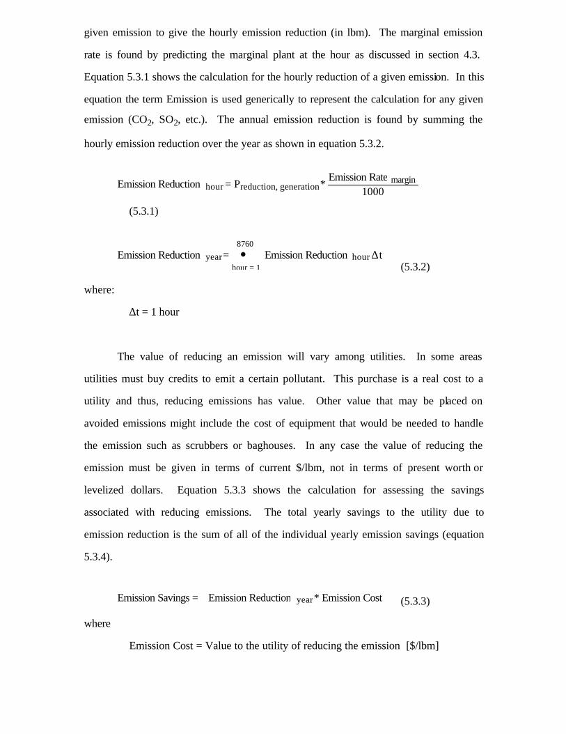
given emission to give the hourly emission reduction (in lbm). The marginal emission
rate is found by predicting the marginal plant at the hour as discussed in section 4.3.
Equation 5.3.1 shows the calculation for the hourly reduction of a given emission. In this
equation the term Emission is used generically to represent the calculation for any given
emission (CO2, SO2, etc.). The annual emission reduction is found by summing the
hourly emission reduction over the year as shown in equation 5.3.2.
Emission Reduction hour = Preduction, generation *
Emission Rate margin1000
(5.3.1)
Emission Reduction year = Emission Reduction hour•
hour = 1
8760 ∆t
(5.3.2)
where:
∆t = 1 hour
The value of reducing an emission will vary among utilities. In some areas
utilities must buy credits to emit a certain pollutant. This purchase is a real cost to a
utility and thus, reducing emissions has value. Other value that may be placed on
avoided emissions might include the cost of equipment that would be needed to handle
the emission such as scrubbers or baghouses. In any case the value of reducing the
emission must be given in terms of current $/lbm, not in terms of present worth or
levelized dollars. Equation 5.3.3 shows the calculation for assessing the savings
associated with reducing emissions. The total yearly savings to the utility due to
emission reduction is the sum of all of the individual yearly emission savings (equation
5.3.4).
Emission Savings = Emission Reduction year * Emission Cost (5.3.3)
where
Emission Cost = Value to the utility of reducing the emission [$/lbm]

Quantifying Utility Costs and Benefits 53
Total Emission Savings = Emission Savings i•
i = 1
# emissions (5.3.4)
5.4 Assessing Demand Reduction and Its Value
The value of reducing demand is identified in three areas. Demand reduction has
value at the generation level as it reduces capacity and reserve requirements. Demand
reduction is also beneficial to the transmission and distribution systems since it lessens
their capacity requirements. The avoided costs of meeting the capacity needs has value
to generation, transmission and distribution systems.
Demand reduction can be assessed using a peak load hour method or the capacity
contribution index (CCI) method. The former method assesses demand reduction as the
avoided generation at a single peak load hour or as the average demand reduction for a
specified number of hours with highest loads. The CCI method assesses demand
contributions over the entire year, weighted by the marginal expected unserved energy
(EUE). The methodologies for assessing demand reduction and its value to a utility of
both approaches are developed in the following sections.
5.4.1 Peak Load Hour Method
The peak load hour method assesses the average demand reduction at a specified
number of peak load hours. The first step in this approach is to identify the peak loads
and the hours at which they occur. Figure 5.4.1-1 shows the twenty highest loads
experienced by WEPCO in 1991 and the hours at which they occur. The solar energy
system demand reductions at these hours are then identified to assess demand

contributions to the generation, transmission and distribution systems.
0
1000
2000
3000
4000
5000
5774
5727
5752
5750
5753
5751
5775
5728
5726
5703
4263
5704
4264
5702
5773
5729
4265
4262
5776
5705
Loa
d [M
W]
hour of year
Figure 5.4.1-1: Peak Loads and Time of Occurrence. WEPCO, 1991
To quantify the reduction in capacity requirements, the solar energy system
performance, as defined in section 5.2, is used. Generation utilities must have enough
capacity to meet the load, overcome transmission and distribution losses and maintain a
certain reserve margin to provide a desired level of reliability. Equation 5.4.1.1 gives the
average reduction in capacity requirements for an electric generation utility due to an
ensemble of solar systems.
Capacityreduction, generation =
Nsystemsnpeak hours
* Psystem, peak houri•i = 1
npeak hours
(1-Lossdistribuiton) * (1-Loss transmission) * (1 + reserve margin)
(5.4.1.1)
where:
npeak hours = the number of peak load hours investigated
Psystem, peak houri = the solar system performance at the peak load hour
reserve margin = the fractional reserve margin of the generation utility
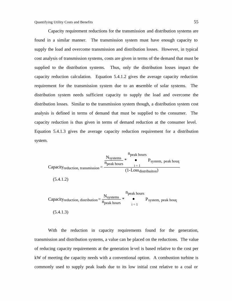
Quantifying Utility Costs and Benefits 55
Capacity requirement reductions for the transmission and distribution systems are
found in a similar manner. The transmission system must have enough capacity to
supply the load and overcome transmission and distribution losses. However, in typical
cost analysis of transmission systems, costs are given in terms of the demand that must be
supplied to the distribution systems. Thus, only the distribution losses impact the
capacity reduction calculation. Equation 5.4.1.2 gives the average capacity reduction
requirement for the transmission system due to an ensemble of solar systems. The
distribution system needs sufficient capacity to supply the load and overcome the
distribution losses. Similar to the transmission system though, a distribution system cost
analysis is defined in terms of demand that must be supplied to the consumer. The
capacity reduction is thus given in terms of demand reduction at the consumer level.
Equation 5.4.1.3 gives the average capacity reduction requirement for a distribution
system.
Capacityreduction, transmission =
Nsystemsnpeak hours
* Psystem, peak houri•i = 1
npeak hours
(1-Lossdistribuiton)
(5.4.1.2)
Capacityreduction, distribution =
Nsystemsnpeak hours
* Psystem, peak houri•i = 1
npeak hours
(5.4.1.3)
With the reduction in capacity requirements found for the generation,
transmission and distribution systems, a value can be placed on the reductions. The value
of reducing capacity requirements at the generation level is based relative to the cost per
kW of meeting the capacity needs with a conventional option. A combustion turbine is
commonly used to supply peak loads due to its low initial cost relative to a coal or

nuclear power plant. Equation 5.4.1.4 gives the value of reducing capacity requirements
to a generation utility.
Demand Savings generation = Capacityreduction, generation * Costconventional option (5.4.1.4)
where:
Costconventional option = the present worth cost of a conventional option [$/kW]
The value to transmission and distribution systems due to demand reductions are
found in a similar manner. The cost used in assessing the value of reducing capacity
requirements is the cost per kW of adding sufficient facilities and equipment to supply
the demand. In the case of the transmission system, the demand is that which is supplied
to the distribution system. In the case of the distribution system, the demand is that
which is supplied to the consumer. The cost is given in present worth dollars per kW.
Equations 5.4.1.5 and 5.4.1.6 give value of reducing capacity requirements to
transmission and distribution systems respectively. Equation 5.4.1.7 gives the value of
the total demand savings due to an ensemble of solar energy systems.
Demand Savings transmission = Capacityreduction, transmission * Costadding capacity (5.4.1.5)
Demand Savings distribution = Capacityreduction, distribution * Costadding capacity (5.4.1.6)
Demand Value = Demand Savingsgeneration + Demand Savingstransmission
+ Demand Savingsdistribution (5.4.1.7)
A capacity reduction ratio (CRR) is defined as the ratio of system performance to
optimal performance. The optimal performance is defined as the maximum possible
system performance. For an SDHW system, the optimal system performance is the
maximum average EDHW system demand. For a PV system, the optimal performance is

Quantifying Utility Costs and Benefits 57
defined as the maximum generation provided by the sys tem. This ratio is calculated at
the peak load hours and averaged. The CRR Equation 5.4.1.8 gives the CRR for a solar
resource. The CRR attempts to estimate the capacity contribution index of the solar
option, as discussed in the following section.
CRR = 1
npeak hours
Psystem, peak houriPoptimal
•i = 1
npeak hours
(5.4.1.8)
5.4.2 Capacity Contribution Index Method
The Capacity Contribution Index (CCI) method of assessing the value of demand
reduction compares the contribution to system reliability of a supply-side or demand-side
resource to that of a conventional resource (Harsevoort and Arny, 1994). Capacity
contributions normalized to the maximum possible (optimal) capacity of the resource are
weighted by the marginal expected unserved energy (EUE) on an hourly basis. The
marginal EUE is a measure of system stress at each hour. The marginal EUE considers
full and partial forced outages of the generation units. Hours with higher marginal EUE
values indicate times of greater stress compared to hours with lower marginal EUE
values. Capacity contributions at hours with higher EUE values have greater significance
to improving system reliability than capacity contributions at hours with lower marginal
EUE values. The marginal EUE values are calculated on a regional basis. The sum of
the hourly marginal EUE values is equal to unity (Harsevoort and Arny, 1994).
Figure 5.4.2-1 shows the marginal EUE values for the utility region containing
WEPCO. The region is made up of interconnected generating facilities in Wisconsin,
Illinois, Iowa, Minnesota, Nebraska, North Dakota, South Dakota and Manitoba

(Harsevoort and Arny, 1994). Hours not shown in the figure have marginal EUE values
of zero. Marginal EUE values of zero indicate times of excess capacity.
0
0.03
0.06
0.09
0.12
0.15
5752
5728
5729
5753
5751
5727
5750
5730
5705
4864
5754
5726
5704
4865
5703
5776
5775
4863
5777
5749
5702
5706
4866
5774
4862
5731
5725
5773
5755
5701
5748
5778
Mar
gina
l EU
E
time
Figure 5.4.2-1: Regional Marginal EUE Values
The first step in assessing the CCI of a solar energy resource is to define an
optimal system performance to normalize the hourly system performance. For an
analysis of an ensemble of SDHW systems, the optimal system performance is defined as
the maximum average demand of an ensemble of EDHW system. For an analysis of an
ensemble of PV systems, the optimal system performance is defined as the maximum
average generation of the PV ensemble. The optimal system performance is a measure of
the maximum possible performance of the system. Normalizing the system performance
to a optimal system performance provides a basis for calculating the hourly CCI values
for solar options.
The marginal CCI values of the solar energy resource are calculated on an hourly
basis. The normalized system performance is weighted by the marginal EUE of the
electric generation region. This weighting of system performance credits capacity
contributions of the solar energy resource at times of higher system stress than
contributions at times of lower system stress. Equation 5.4.2.1 gives the marginal CCI

Quantifying Utility Costs and Benefits 59
for a solar resource.
CCIsolar, marginal =
PsystemPoptimal
* EUEmarginal (5.4.2.1)
The sum of the marginal CCI values over the entire year gives the CCI of the
solar resource (equation 5.4.2.2). The CCI of the resource given in equation 5.4.2.2
indicates the contribution to system reliability of the resource. As defined, the CCI will
range between 0 and 1. If the resource provides its optimal capacity at each hour, its CCI
will be unity since the marginal EUE values add to unity. When the resource provides
less than its optimal capacity at times throughout the year, its CCI will be less than 1.
CCIsolar = CCIsolar, marginal i•
i = 1
8760
(5.4.2.2)
The CCI of the solar resource is used to compare its contribution to system
reliability versus that of a conventional option that would contribute the same amount of
optimal capacity. Relative reliability improvements are assessed for generation,
transmission and distribution systems. The same considerations are used in calculating
the capacity reductions for each system as described in section 5.4.1. Equations 5.4.2.3,
5.4.2.4 and 5.4.2.5 give the capacity reduction requirements for the generation,
transmission and distribution systems respectively. The value assessed through these
equations is the equivalent kW of a conventional option provided by the solar system.
For example if the conventional option used for comparison is a combustion turbine, the
equations give the amount of equivalent combustion turbine capacity that is displaced
with the solar resource.
Capacityreduction, generation =

CCIsolar
CCIconventional * Poptimal ⋅ Nsystems * 1 + reserve margin
(1-Lossdistribution) * (1-Losstransmission)
(5.4.2.3)
Capacityreduction, transmission = CCIsolarCCIconventional
* Poptimal ⋅ Nsystems1-Lossdistribution
(5.4.2.4)
Capacityreduction, distribution = CCIsolar
CCIconventional *Poptimal⋅ Nsystems
(5.4.2.5)
The CCI method allows for placing value on demand reduction in terms of the
cost of a conventional reference option. The capacity displacements, given in terms of
kW, reflect the amount of capacity reduction of an ensemble of solar energy systems.
The cost used to quantify the demand savings to the generation utility is the cost of the
reference option per kW since the reference option is the resource being displace. The
cost is given in terms of present worth $/kW. The cost used to quantify demand savings
to the transmission and distribution systems is the marginal cost of supplying a kW. The
cost used for placing value on demand reduction to a transmission system is that of
adding sufficient facilities to supply an added kW to the distribution system, given in
present worth $/kW. The cost used to quantifying demand savings to a distribution
system is that of adding the necessary facilities to supply an added kW to the consumer.
Equations 5.4.2.6, 5.4.2.7 and 5.4.2.8 give the value of demand reduction to the
generation, transmission and distribution systems respectively. Equation 5.4.2.9 gives
the value of the total demand savings due to an ensemble of solar energy systems
Demand Savings generation = Capacityreduction, generation * Costconventional option (5.4.2.6)
Demand Savings transmission = Capacityreduction, transmission * Costadding capacity (5.4.2.7)
Demand Savings distribution = Capacityreduction, distribution * Costadding capacity (5.4.2.8)

Quantifying Utility Costs and Benefits 61
Demand Value = Demand Savingsgeneration + Demand Savingstransmission
+ Demand Savingsdistribution (5.4.2.9)
5.5 Assessing the Value of Other Benefits
Identifying other benefits of a large scale implementation of solar energy systems
is discussed in section 2.2. Other benefits identified are government incentives, customer
retention and delayed power plant construction. This section assesses the value of these
benefits.
Government incentives are often offered for investment in renewable resources.
For example, a tax credit may be given towards the initial investment. Equation 5.5.1
gives the total value of a tax credit towards the investment in solar energy systems. The
credit given by the government is on the order of 10 percent of the investment. The
government may also offer a subsidy for energy produced by a renewable resource.
Equation 5.5.2 gives the total value of the energy subsidy. Typical government subsidies
are on the order of 0.01 - 0.02 $/kWh.
Tax Credit = Investment * % government credit
100 (5.5.1)
Subsidy = Ereduction,generation * government subsidy (5.5.2)
A solar DSM program may increase the market of an electric utility through
customer retention or capturing new markets. Customer retention is defined as the
difference in the number of customers lost to an alternative fuel without the solar
program and those which are lost with the program. Equation 5.5.3 can be used to place
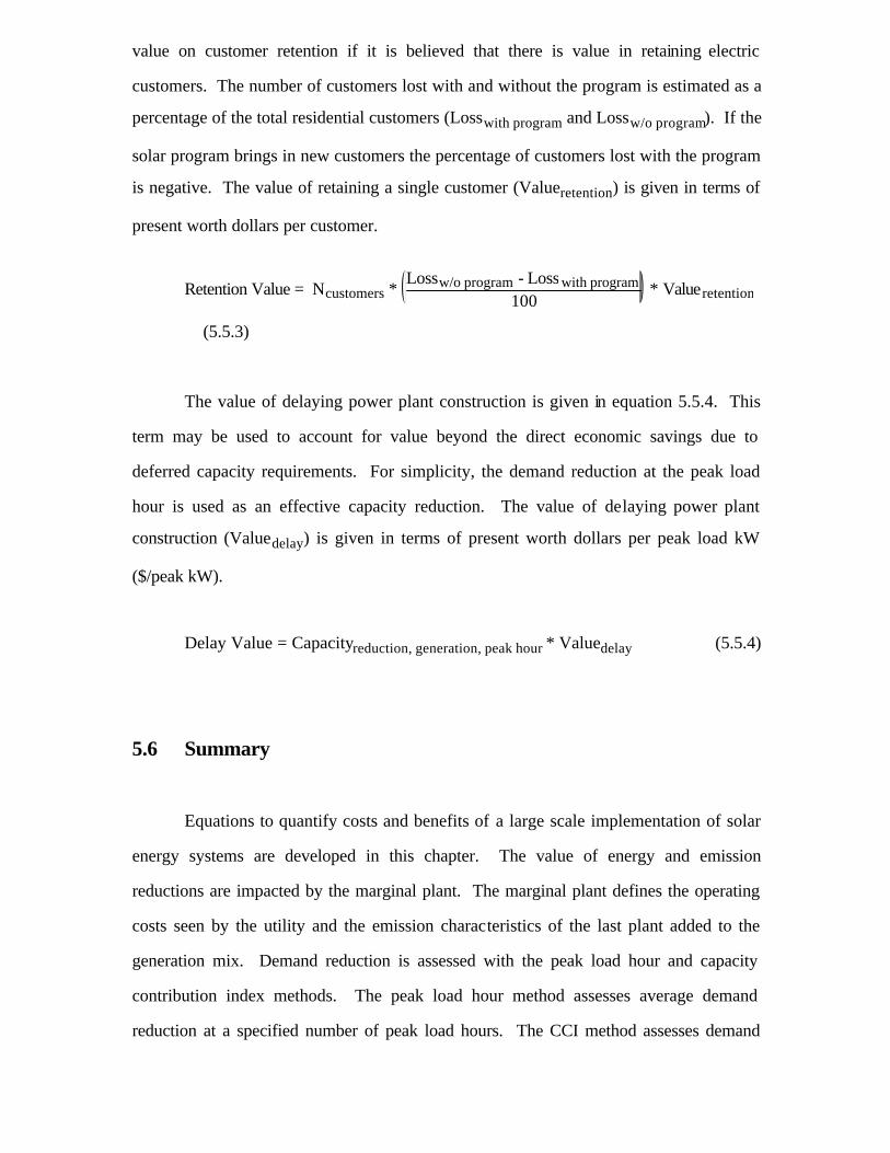
value on customer retention if it is believed that there is value in retaining electric
customers. The number of customers lost with and without the program is estimated as a
percentage of the total residential customers (Losswith program and Lossw/o program). If the
solar program brings in new customers the percentage of customers lost with the program
is negative. The value of retaining a single customer (Valueretention) is given in terms of
present worth dollars per customer.
Retention Value = Ncustomers *
Lossw/o program - Losswith program100
* Valueretention
(5.5.3)
The value of delaying power plant construction is given in equation 5.5.4. This
term may be used to account for value beyond the direct economic savings due to
deferred capacity requirements. For simplicity, the demand reduction at the peak load
hour is used as an effective capacity reduction. The value of delaying power plant
construction (Valuedelay) is given in terms of present worth dollars per peak load kW
($/peak kW).
Delay Value = Capacityreduction, generation, peak hour * Valuedelay (5.5.4)
5.6 Summary
Equations to quantify costs and benefits of a large scale implementation of solar
energy systems are developed in this chapter. The value of energy and emission
reductions are impacted by the marginal plant. The marginal plant defines the operating
costs seen by the utility and the emission characteristics of the last plant added to the
generation mix. Demand reduction is assessed with the peak load hour and capacity
contribution index methods. The peak load hour method assesses average demand
reduction at a specified number of peak load hours. The CCI method assesses demand

Quantifying Utility Costs and Benefits 63
reduction in terms of a conventional reference resource. Equations are developed to
assess the values of other benefits including government incentives, customer retention
and delayed power plant construction.
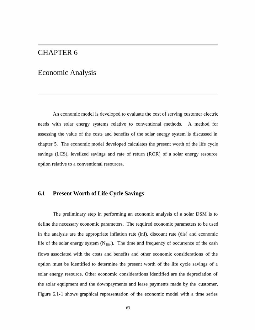
63
CHAPTER 6 Economic Analysis
An economic model is developed to evaluate the cost of serving customer electric
needs with solar energy systems relative to conventional methods. A method for
assessing the value of the costs and benefits of the solar energy system is discussed in
chapter 5. The economic model developed calculates the present worth of the life cycle
savings (LCS), levelized savings and rate of return (ROR) of a solar energy resource
option relative to a conventional resources.
6.1 Present Worth of Life Cycle Savings
The preliminary step in performing an economic analysis of a solar DSM is to
define the necessary economic parameters. The required economic parameters to be used
in the analysis are the appropriate inflation rate (inf), discount rate (dis) and economic
life of the solar energy system (N life). The time and frequency of occurrence of the cash
flows associated with the costs and benefits and other economic considerations of the
option must be identified to determine the present worth of the life cycle savings of a
solar energy resource. Other economic considerations identified are the depreciation of
the solar equipment and the downpayments and lease payments made by the customer.
Figure 6.1-1 shows graphical representation of the economic model with a time series

64
representation of the considered cash flows. The terms A, B, C and D represent
combined cash flows of the costs and benefits from a solar DSM program.
A
D
0 1Ndepreciation
Nlife
Given: inf & dis
B C B C B C
D
Figure 6.1-1: The Economic Model
The cash flows are categorized by their occurrence and how they are handled in the economic
calculation. Equation 6.1.1 gives the present worth of the life cycle savings of a solar energy option
relative to a conventional option.
LCSPW = A + B*PWF(Nlife,inf,dis) + C*PWF(Nlife,0,dis)
+ D*PWF(Ndepreciation,0,dis) (6.1.1)
where:
A = -Investment + Tax Credit + Demand Value + Delay Value + Retention Value
+ Downpayments
B = Energy Savings + Total Emission Savings + Subsidy - OM&A
C = Lease Payments (monthly lease payment *12)
D = Depreciation
inf = inflation rate
dis = discount rate
Nlife = economic life of solar energy system
Ndepreciation = number of years of equipment depreciation schedule

Economic Analysis 65
The parameters that make up the A term in equation 6.1.1 are credited for a time
zero. The investment and associated government tax credit and customer downpayments
are assumed to occur immediately. The value of demand is given as the cost in present
dollars of an option that would supply an equivalent amount of demand that is provided
by the solar energy systems. A common example of such an option is a combustion
turbine. Similarly, delaying the construction of new facilities is credited for in present
worth dollars. This term accounts for any additional value of demand reduction beyond
capacity contributions such as the ability to invest money that would be needed to pay for
the new facilities. Customer retention is also credited for at time zero in terms of present
worth dollars.
The series of benefits that make up the B term in equation 6.1.1 are brought back
to present time with the present worth factor (equation 6.1.2) using the parameters Nlife,
inf and dis (Duffie and Beckman, 1991). The present worth factor term is represented in
equation 6.1.1 as PWF(Nlife,inf,dis). The terms in this series of benefits are assumed to
inflate over the life of the option.
PWF(N,i,d) = 1
(d-i)* 1 - 1+i
1+dN
if i ≠ d
PWF(N,i,d) = N
(i+1) if i = d (6.1.2)
The series of lease payments (term C) are brought back to present value using the
present worth factor PWF(Nlife,0,dis). The economic calculation is simplified by
assuming that the utility sees an annual lease payment rather than monthly payments. It
is assumed that the customer will pay the same monthly payment over the life of the
program. That is, the lease payment does not inflate.
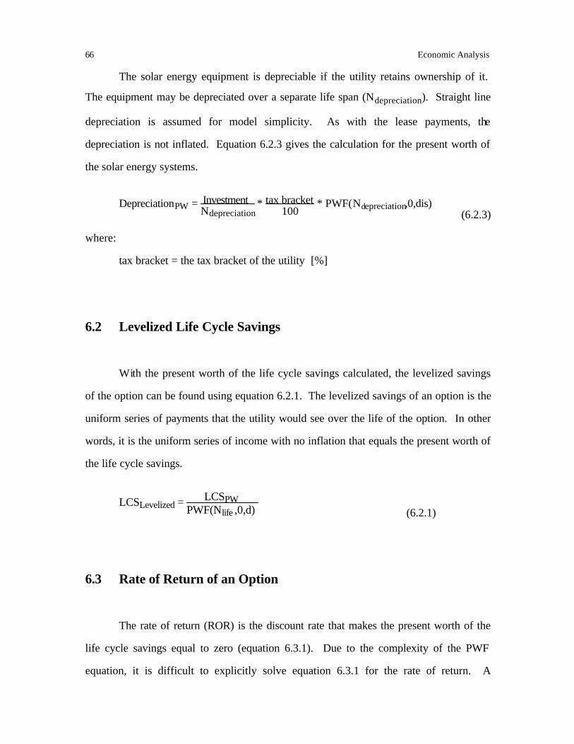
66 Economic Analysis
The solar energy equipment is depreciable if the utility retains ownership of it.
The equipment may be depreciated over a separate life span (Ndepreciation). Straight line
depreciation is assumed for model simplicity. As with the lease payments, the
depreciation is not inflated. Equation 6.2.3 gives the calculation for the present worth of
the solar energy systems.
DepreciationPW = Investment
Ndepreciation * tax bracket
100 * PWF(Ndepreciation,0,dis)
(6.2.3)
where:
tax bracket = the tax bracket of the utility [%]
6.2 Levelized Life Cycle Savings
With the present worth of the life cycle savings calculated, the levelized savings
of the option can be found using equation 6.2.1. The levelized savings of an option is the
uniform series of payments that the utility would see over the life of the option. In other
words, it is the uniform series of income with no inflation that equals the present worth of
the life cycle savings.
LCSLevelized = LCSPW
PWF(Nlife ,0,d) (6.2.1)
6.3 Rate of Return of an Option
The rate of return (ROR) is the discount rate that makes the present worth of the
life cycle savings equal to zero (equation 6.3.1). Due to the complexity of the PWF
equation, it is difficult to explicitly solve equation 6.3.1 for the rate of return. A

Economic Analysis 67
numerical method is used to solve the rate of return.
0 = A + B*PWF(Nlife,inf,ROR) + C*PWF(Nlife,0,ROR)
+ D*PWF(Ndepreciation,0,ROR) (6.3.1)
The rate of return is found using Newton’s method. Figure 6.3-1 displays the
process graphically. The present worth of the option is found with the discount rate used
by the utility. This calculation gives point A in figure 6.3-1. The derivative of the
LCSPW curve with respect to the discount rate, as at point A, is given by equation 6.3.2.
dLCSPW
dd = B*ŽPWF(Nlife ,inf,d)
Žd + C*ŽPWF(Nlife ,0,d)
Žd + D*
ŽPWF(Ndepreciation,0,d)Žd
(6.3.2)
The partial derivative of the present worth factor with respect to the discount rate
(ŽPWF(N,i,d)
Žd ) is given by equation 6.3.3.
ŽPWF(N,i,d)
Žd= N
(1+d) * 1+i
1+dN - PWF(N,i,d)
d-i if i ≠ d
ŽPWF(N,i,d) Žd
= -N1+d 2 if i = d (6.3.3)
A new discount rate (dnew) is found by equating the derivative evaluated at point A to the
slope of the line computed with point A and a present worth of zero.
dLCSPW
dd = 0 - LCSPW
dnew - dold
Rearranging the equation becomes equation 6.3.4.

68 Economic Analysis
dnew = -LCSPW
dLCSPW/dd + dold
(6.3.4)
This new discount rate is used to re-evaluate the present worth (point B in figure 6.3-1)
and the process is repeated. A tolerance is placed on the present worth. Once the
evaluation of the present worth is less than the tolerance, the iteration is stopped and the
last value of dnew is the rate of return (point N in figure 6.3-1).
LCSPW
ddis ROR
A
B
N
Figure 6.3-1: Graphical Representation of ROR Calculation Process
6.4 Summary
An economic model is developed to assess the savings of a solar energy DSM
program. An equation that calculates the life cycle savings of the cost of serving the
customer with solar energy systems relative to an entirely central generation option is
developed. The economic model accounts for the costs and benefits discussed in chapter
5 as well as customer payments towards the systems and equipment depreciation. An
equation to calculate the levelized life cycle savings and a method to find the rate of
return are developed.

70
CHAPTER 7 Case Study
The software package EUSESIA, An Electric Utility Solar Energy System Impact
Analysis (Trzesniewski et al., 1995) is used in a case study. EUSESIA employs the
models and equa tions developed to this point to automate the analysis of the impact of an
ensemble of solar energy systems on an electric utility. EUSESIA is broken down into
three general areas of analysis: solar energy and conventional system analysis, marginal
plant analysis and economic and environmental impact analysis.
A group of subprograms predicts the electric demands of solar and electric
domestic hot water systems and the electric generation of a photovoltaic system. These
system performances are calculated on an hourly basis for an entire year. Generic system
parameters are supplied, but the user can modify the system parameters. With expertise
in TRNSYS, specific solar systems that are being considered in demand-side
management programs can be simulated and added to the EUSESIA analysis.
A second subprogram determines the marginal utility plant on an hourly basis given specific plant
data and hourly load. The marginal plant is found on a least cost basis. The user has the ability to input
data for their plant mix or regional plant data that includes neighboring utilities. The latter results in a more
realistic analysis as it better represents a real market in which utilities buy and sell energy and capacity
from their neighbors.
Finally, an economic and environmental impact analysis program performs calculations using
information about system performance and about the marginal plant. Energy, emission and demand

Case Study 71
reductions are quantified in terms of both physical quantities and dollars. These savings are used with the
other economic benefits previously discussed to calculate the life cycle savings of the option.
7.1 Solar Energy System Performance
A one tank SDHW and a PV system are simulated to assess system performance.
The default SDHW system parameters used in the simulation are summarized in table
3.1.1.2-1. The SDHW system performance is based relative to an EDHW system with
default system parameters as those summarized in table 3.1.1.1-1. The default PV system
parameters used in the simulation are summarized in table 3.2-2. The PV panel
parameters used in the simulation are those of the Advanced Photovoltaic Systems Inc.
EP-50 (table 3.2-1). The solar systems are simulated using 1991 weather data for
Milwaukee, Wisconsin.
Figure 7.1-1 shows the average hourly demands of SDHW and EDHW systems
with the default system parameters. The average system performance of the SDHW
system is defined as the difference between the EDHW and SDHW demands. Figure 7.1-
2 shows the average power generation of the default PV system. These system
performances are used later for assessing the impact at the generation level.

0
0.5
1
1.5
2
0 2000 4000 6000 8000
EDHW DemandSDHW Demand
Ele
ctri
c D
eman
d [k
W]
time [hour]8760
Figure 7.1-1: SDHW and EDHW System Demands
0
0.05
0.1
0.15
0.2
0.25
0 2000 4000 6000 8000
Ele
ctri
c G
ener
atio
n [k
W]
time [hr]8760
Figure 7.1-2: PV System Generation
Monthly system performance is assessed to show reductions in customer
electricity use. The average demand reductions of the SDHW system and the average
generation of the PV system are integrated monthly. Figure 7.1-3 shows the difference in
monthly average customer electricity consumption for hot water heating between SDHW
and EDHW systems. Figure 7.1-4 depicts the monthly average reduction in electricity
consumption for a household with a PV system. Although the PV system generation is
assumed to be connected to the grid, the electrical generation could be used by the

Case Study 73
household. The use of the generated electricity would result in a reduction in the use of
utility generated electricity.
0
100
200
300
400
500
J F M A M J J A S O N D
Ene
rgy
Red
uctio
n [k
Wh]
month
Figure 7.1-3: Average SDHW System Energy Use Reduction
0
5
10
15
20
25
30
35
J F M A M J J A S O N D
Ene
rgy
Red
uctio
n [k
Wh]
month
Figure 7.1-4: Average PV System Energy Use Reduction
Consumer electric bill savings are quantified with the energy reductions from the
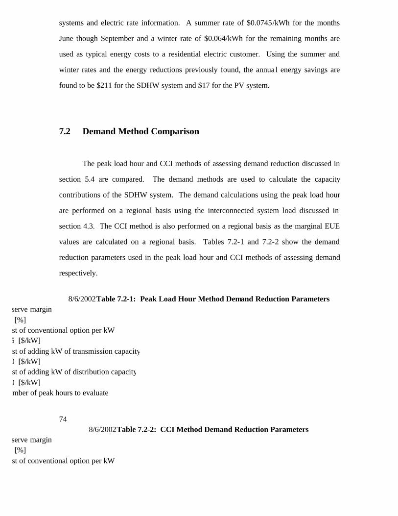
systems and electric rate information. A summer rate of $0.0745/kWh for the months
June though September and a winter rate of $0.064/kWh for the remaining months are
used as typical energy costs to a residential electric customer. Using the summer and
winter rates and the energy reductions previously found, the annua l energy savings are
found to be $211 for the SDHW system and $17 for the PV system.
7.2 Demand Method Comparison
The peak load hour and CCI methods of assessing demand reduction discussed in
section 5.4 are compared. The demand methods are used to calculate the capacity
contributions of the SDHW system. The demand calculations using the peak load hour
are performed on a regional basis using the interconnected system load discussed in
section 4.3. The CCI method is also performed on a regional basis as the marginal EUE
values are calculated on a regional basis. Tables 7.2-1 and 7.2-2 show the demand
reduction parameters used in the peak load hour and CCI methods of assessing demand
respectively.
8/6/2002Table 7.2-1: Peak Load Hour Method Demand Reduction Parameters
Reserve margin 15 [%] Cost of conventional option per kW 325 [$/kW] Cost of adding kW of transmission capacity 100 [$/kW] Cost of adding kW of distribution capacity 100 [$/kW] Number of peak hours to evaluate
74 8/6/2002Table 7.2-2: CCI Method Demand Reduction Parameters
Reserve margin 15 [%] Cost of conventional option per kW

Case Study 75
325 [$/kW] Cost of adding kW of transmission capacity 100 [$/kW] Cost of adding kW of distribution capacity 100 [$/kW] CCI of conventional option 0.92
75
A typical reserve margin of 15% is used in both methods. The cost of the
conventional option is given in present worth dollars per kW. This cost is representative
of a combustion turbine as this is a common generation resource used to meet demand in
times of high system stress. The CCI value of the combustion turbine is taken from A
Method for Comparing the Contribution of Supply-Side and Demand-Side Resources to
Customer Reliability (Harsevoort and Arny, 1994). The costs of adding an additional kW
of transmission and distribution capacity are given in present worth dollars per kW.
The demand analysis is performed for 5000 solar energy systems. Table 7.2-3
shows the assessment of demand reduction given by the peak load hour and CCI
methods. The demand savings are reported at the end of the first year.
8/6/2002Table 7.2-3: Peak Load Hour and CCI Method Demand Assessments
Method Peak Load Hour
CCI Capacity Contribution [kW]
3490 3529
Total Demand Savings $119,800 $121,200
75 The peak load hour method and CCI method give nearly the same results in assessing capacity
contribution and demand savings. The CCI method is a more rigorous method than the peak load hour method. The CCI method is chosen as the method of demand assessment to be used in further analysis. Marginal EUE data may not be available in all areas, so the CCI method cannot be used. The peak load hour method will provide adequate demand

assessment in such a case.
7.3 Isolated System Versus Interconnected System Analysis
The energy and emission savings of an ensemble of solar energy systems is
directly related to the marginal plant at each hour of the year. What may not be as
obvious is that the magnitude of the impact is affected by the defined system under
investigation. Section 4.3 discusses the marginal plant predictions for WEPCO as an
isolated system and an interconnected system. Energy and emission reductions and the
resulting savings from an ensemble of 5000 SDHW systems are calculated for the
isolated and interconnected systems. Tables 7.3-1 and 7.3-2 show the energy and
emission impacts on an isolated and interconnected system respectively.
8/6/2002Table 7.3-1: Energy and Emission Impacts on an Isolated System
Energy Reduction [kWh] Energy Savings [$]
16,090,000
323,200
Emission Reduction [lbm] Emission Savings [$]
CO2
33,600,000 0
SO2
210,600 4,212 NOX
72,550 0
N2O
565 0
Particulates 4,688

Case Study 77
0 CH4 533 0 77
8/6/2002Table 7.3-2: Energy and Emission Impacts on an Interconnected System
Energy Reduction [kWh] Energy Savings [$]
16,090,000 261,300
Emission Reduction [lbm] Emission Savings [$]
CO2
18,860,000 0
SO2 139,700 2,793 NOX
92,770 0
N2O 298 0
Particulates 7,961
0 CH4
184 0
77
Energy reduction is the same for both cases as it is dependent on the system
performance and transmission and distribution losses and not on the marginal plant. The
savings due to energy reduction is greater for the isolated system than for the

interconnected system because purchases between utilities are neglected. Plants with
higher marginal costs than necessary are being dispatched to meet the load. Artificially
high marginal operating costs are especially apparent in the maintenance periods as
shown in section 4.3.
In general, the emission reduc tions are greater in the isolated system than in the
interconnected system because, in the isolated system, plants with higher emission rates
are forced to be on sooner than would be required in the interconnected system. In the
interconnected system, a greater supply of nuclear plants and cleaner coal plants are
available for dispatch. These plants generally have lower operating costs and are
therefore added to the generating mix before the higher cost plants with poor emission
characteristics. SO2 is the only emission for which credit is taken in this analysis. SO2 is
valued for at $0.02/lbm.
The magnitude of the energy and emission impact is affected by the system under
investigation. The interconnected utility system represents a more realistic environment
in which utilities buy and sell energy. The interconnected system analysis will be used in
further analysis.
7.4 Utility Impact Results
The impact of an ensemble of SDHW systems is assessed for WEPCO. The
analysis is performed on a regional basis and is based on 5000 SDHW systems. Figure
7.4-1 depicts the EUSESIA input file which shows the specific parameters used in the
analysis.
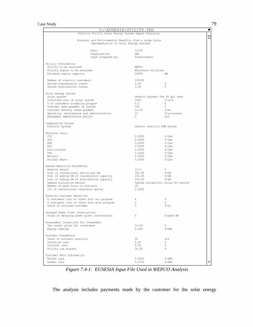
Case Study 79
C:\EUSESIA\UTILITY.TRDElectric Utility Solar Energy System Impact Analysis:
Economic and Environmental Benefits from a Large Scale
Implementation of Solar Energy Systems
Date: 12/95 Organization: SEL Input prepared by: Trzesniewski Utility Information Utility to be analyzed WEPCO Utility region to be analyzed Wisconsin Utilities Estimate region capacity 20000 MW Number of electric customers 100000 System transmission losses 2.00 % System distribution losses 3.00 % Solar Energy System Solar system Generic System: One 80 gal tank Installed cost of solar system 2000 $/unit % of customers accepting program 5.0 % Customer down payment on system 140 $ Customer monthly lease payment 12.00 $/mo Operation, maintenance and administration 10 $/yr-system Equipment depreciation period 5 yrs Comparative System Electric System Generic electric DHW system Emission Costs CO2 0.0000 $/lbm SO2 0.0200 $/lbm NOX 0.0000 $/lbm N2O 0.0000 $/lbm Particulates 0.0000 $/lbm CH4 0.0000 $/lbm Mercury 0.0000 $/lbm Nuclear Waste 0.0000 $/lbm Demand Reduction Parameters Reserve margin 15.0 % Cost of conventional option per kW 325.00 $/kW Cost of adding kW of transmission capacity 100.00 $/kW Cost of adding kW of distribution capacity 100.00 $/kW Demand evaluation method System reliability using CCI method Number of peak hours to evaluate 20 CCI of conventional reference option 0.9200 Electric Customer Retention % customers lost to other fuel w/o program 4 % % customers lost to other fuel with program 2 % Value of retained customer 0 $/yr Delayed Power Plant Construction Value of delaying power plant construction 0 $/peak kW Government Incentives for Investment Tax credit given for investment 10.00 % Energy subsidy 0.000 $/kWh Economic Parameters Years of economic analysis 20 yrs Inflation rate 5.00 % Discount rate 8.00 % Utility tax bracket 34.00 % Customer Rate Information Winter rate 0.0640 $/kWh Summer rate 0.0745 $/kWh
Figure 7.4-1: EUSESIA Input File Used in WEPCO Analysis
The analysis includes payments made by the customer for the solar energy

systems. For example, a program by WPS offers the solar systems to the customer for
$140 down and a $12 per month lease. The installed cost of a single solar energy system
is $2000. The utility is assumed to maintain ownership of the systems so that they may
be depreciated. The depreciation period chosen is five years.
A utility may have reasons to credit emissions with a certain value. SO2 has real
value as WEPCO must buy credits to emit SO2. The value assigned to SO2 is $0.02/lbm. No
other emissions are credited for in this analysis.
The CCI method is used to evaluate demand reduction. Capacity contributions at
the generation level are valued relative to a combustion turbine. The present worth value
of capacity contribution is given to be $325/kW. Transmission and distribution capacity
contributions are each given a present worth value of $100/kW. This is the cost of
adding an additional kW of capacity in each of the systems.
Customer retention and delayed power plant construction are not credited for in
this analysis. Government incentives, however are included as benefits of the solar
program. A ten percent tax credit is given for the initial investment in purchasing the
solar energy systems.
The economic parameters are chosen to best represent WEPCO. The economic
life of the SDHW systems is given as 20 years. An inflation rate of 5% and a discount
rate of 8% are used in the economic calculations. The utility is assumed to be in the 34%
taxbracket. Figure 7.4-2 shows the outputs from the EUSESIA analysis.

Case Study 81
C:\EUSESIA\UTILITY.OUT
Electric Utility Solar Energy System Impact Analysis:
Impact of a Large Scale Implementation of a Solar Energy System on an Electric Utility
** Energy and Environmental Impact Summary for the First Year ****** Results based on: 5000 solar systems Energy Reduction (kWh) Energy Savings ($) 16090000 261300 Emission Reduction (lbm) Emission Value ($) CO2 18860000 0 SO2 139700 2793 NOX 92770 0 N2O 298 0 Parts 7961 0 CH4 184 0 HG 0 0 NUKES 0 0 2793 Demand Reduction (kW) Demand Savings ($) 3529 121200 Total Savings ($) 385293 ** Economic Analysis Summary *************************************** Present Worth of Investment - $ 10000000 Present Worth of OM&A - $ 717900 Present Worth of Energy Savings $ 3751000 Present Worth of Emission Savings $ 40110 Present Worth of Demand Savings $ 1740000 Present Worth of Depreciation $ 2715000 Present Worth of Downpayments $ 700000 Present Worth of Lease Payments $ 7069000 Present Worth of Tax Credit $ 1000000 Present Worth of Energy Subsidy $ 0 Present Worth of Customer Retention $ 0 Present Worth of Delay Value $ 0 Present Worth of Life Cycle Savings $ 6297000 Levelized Savings of Option $ 641400 Rate of Return of Option 21.2 % ** System Performance Summary and Customer Savings ***************** Results based on average system performance Elc (kWh) Sol (kWh) Del (kWh) SF Savings ($) JAN 489 357 132 .269 8.43 FEB 437 262 174 .399 11.16 MAR 477 256 221 .463 14.13 APR 449 157 293 .651 18.73 MAY 459 114 345 .753 22.09 JUN 439 40 399 .909 29.69 JUL 444 51 393 .885 29.27 AUG 444 72 371 .837 27.65 SEP 442 135 307 .695 22.87 OCT 463 252 212 .457 13.55 NOV 458 352 106 .230 6.75 DEC 478 370 109 .227 6.95 YEAR 5477 2417 3060 .559 211.28 Option Capacity Contribution Index .378
Figure 7.4-2: EUSESIA Output File from WEPCO Analysis
The energy and environmental impact summary gives the energy, emission and

demand reductions and the resulting savings at the end of the first year of the analysis.
The demand reduction reported does not include capacity contributions in the
transmission and distribution systems, only capacity contributions at the generation level.
The demand savings, however, do include the value of the capacity contribution to the
transmission and distribution systems. The energy, emission and demand savings can be
used as yearly recurring savings in an economic calculation.
Normalizing the energy, emission and demand reductions to the number of
systems used in the analysis gives the average impact of a single SDHW system at the
generation level. Table 7.4-1 shows the average impact of an SDHW system at the
generation level.
Table 7.4-1: Average Impact of an SDHW System at the Generation Level
Energy Reduction [kWh] 3218
Emission Reduction [lbm]
CO2 3772 SO2 27.9 NOX 18.6 N2O 0.0596 Particulates 1.6 CH4 0.0368
Demand Reduction [kW]
.71
The present worth of the life cycle savings for the SDHW option is around 6.3
million dollars. Levelized, the life cycle savings are $641,400 per year. The rate of
return of the SDHW ensemble is 21.2%. A similar analysis including only the cost of the
systems, operation and maintenance costs and the energy, emission and demand savings
results in a rate of return of 2.8%. The results of the economic calculation are therefore
sensitive to the benefits for which credit is taken.

Case Study 83
The system performance summary gives results based on average system
performance and therefore are of interest to a typical customer. The energy requirements
of the EDHW and SDHW systems and their difference are given on a monthly basis. The
annual solar fraction (SF) of the SDHW system is defined to be the difference in the
EDHW and SDHW energy requirements divided by the EDHW energy requirement. The
solar fraction is found to be 0.56. The monthly savings are reported using the seasonal
rate information discussed in section 7.1. The annual savings to a customer is $211. The
capacity contribution index discussed in section 5.4 is calculated to be 0.378.
An analysis performed for an ensemble of 5000 PV systems similar to the one
discussed in section 7.1, using the same input data as for the SDHW system analysis,
gives annual energy savings of $21,860, emission savings of $243 and demand savings of
$18,190. The rate of return calculated for the PV system is 10.8%. The average impact
of a PV system at the generation level is given in table 7.4-2.
Table 7.4-2: Average Impact of a PV System at the Generation Level
Energy Reduction [kWh] 262
Emission Reduction [lbm]
CO2 344 SO2 2.43 NOX 1.45 N2O 0.0054 Particulates 0.131 CH4 0.0038
Demand Reduction [kW]
.10

7.5 Summary
The software package EUSESIA is used to simulate SDHW and PV system
performance and to assess the impact of an ensemble of 5000 SDHW systems on
WEPCO. The CCI method of demand assessment is chosen to quantify capacity
contributions. A regional analysis, considering WEPCO as an interconnected utility, is
chosen for the study. The study shows energy reductions at the generation level to be
slightly over 16 Gigawatt hours. Emission reductions are quantified and the total demand
reduction is shown to be 3529 kW. The average capacity contribution is 0.71 kW per
system. The SDHW system saves a consumer $211 per year on electric bills. A similar
study for a PV system shows about 1.7 Gigawatt hours of energy reduction and a demand
reduction of 530 kW. The PV system saves a consumer approximately $17 per year on
electric bills. SDHW systems have a larger impact on a utility than PV systems with
comparable array areas. SDHW systems also offer consumers greater savings on electric
bills. When considering only the energy, emission and demand savings and costs of the
system and operation and maintenance, the rate of return is calculated to be 2.8%. By
including customer payments, equipment depreciation and government incentives in the
economic analysis gives a rate of return of 21.2%.

86
CHAPTER 8 Conclusions and Recommendations
8.1 Conclusions
A large scale implementation of solar energy systems has significant impact on an
electric utility. On average, an SDHW system consisting of a 60 ft2 collector and a single
80 gallon tank realizes annual energy reductions at the utility level of 3218 kWh,
emission reductions of: 3772 lbm CO2, 27.9 lbm SO2, 18.6 lbm NOX, 0.0596 lbm N2O,
1.6 lbm particulates and 0.0368 lbm CH4 and demand reduction of 0.71 kW. A PV
system of comparable array area shows substantially less impact.
The annual savings resulting from an ensemble of 5000 SDHW systems are
$261,300 in energy reduction, $2,793 in emission reduction and $121,200 in demand
reduction. The emission savings are negligible compared to the energy and demand
savings, but may be more substantial in the future as emission regulations become
tougher.
An economic analysis shows the rate of investment to be 2.8% when considering only the
energy, emission and demand savings and the costs of the systems and annual operation
and maintenance costs. When customer payments, equipment depreciation and
government incentives are included in the economic analysis, however, the rate of
investment is calculated to be 21.2%. The results of economic analysis are dependent on
the benefits for which the utility takes credit.
An annual analysis performed on an hourly basis is required to accurately assess
the impact of an ensemble of solar energy systems on an electric utility. Energy savings

87
and emission reduction are dependent on the operating costs and emission characteristics
of the marginal plant, which varies hourly. Hourly weather and load data from the same
year must be supplied to accurately assess the demand reduction of an ensemble of solar
energy systems. For most accurate results, the analysis should be performed on a
regional basis. Considering the utility as part of an interconnected system of utilities
represents a more realistic environment, in which utilities buy and sell energy and
demand from one another, than considering the utility as an isolated system.
8.2 Recommendations
The analysis in this research is performed with weather and load information from
1991. It would be useful to perform the analysis with weather and load information from
other years to see if the analyses yield similar results. A database containing hourly
weather data for various locations throughout the country would be useful for assessing
solar performance in other areas. A database containing hourly load and plant data for all
utilities, similar to that of the Federal Energy Regulatory Commission, would help
utilities gather the necessary information to perform regional analyses.
An accessible library containing models of other solar energy system
configurations would offer a user an analysis of more detailed solar energy systems. A
model has been developed to assess demand requirements of a solar energy system
containing collectors rated by the Solar Rating & Certification Corporation (SRCC). A
file containing the parameters of a few SRCC rated collectors is available with the model.
This file could be modified to contain all the collectors rated by the SRCC.
The analysis is not limited to demand-side resources. The impact of a supply-side
resource, such as a wind turbine, could be assessed with EUSESIA. A model producing
hourly wind turbine generation is required for the analysis. Transmission and distribution
losses are not considered when assessing a supply-side resource. Similar to the PV

analysis there would be no comparative system in assessing wind turbines as it is a
generating resource.

175
BIBLIOGRAPHY
Cragan, K.E., Impact on a Utility of an Ensemble of Solar Domestic Hot Water Systems. M.S. Thesis, University of Wisconsin-Madison, 1993. Duffie, J.A. and W.A. Beckman, Solar Engineering of Thermal Processes 2nd Edition. John Wiley & Sons, 1991. Fiksel, A. et al. TRNSHELL: A Menu-Driven Environment Program for TRNSYS, Version 1.0. Solar Energy Laboratory, University of Wisconsin - Madison. July, 1994. Electric Power Research Institute (EPRI). WATSIM User’s Manual Version 1.0. October, 1992. Grater, J., Impact of Distributed Systems. M.S. Thesis, University of Wisconsin- Madison, 1992. Harsevoort, R.J. and M.D.Arny, A Method for Comparing the Contribution of Supply- Side and Demand-Side Resources to Customer Reliability. 1994 Klein, S.A. et al. TRNSYS: A Transient System Simulation Program, Version 14.1. Solar Energy Laboratory University of Wisconsin - Madison. July, 1994. Public Service Commission of Wisconsin. Advance Plan 7, Technical Support Document D24: Power Supply. January 1994. Sinos, N., P.W. Lind, and J. Kirby, “Residential Solar Water Heating Presentation”. Central Vermont Public Service Corporation,.USH2O Utility User Group, January 17, 1995. Solar Rating & Certification Corporation (SRCC), Directory of SRCC Certified Solar Collector and Water Heating System Ratings. Washington D.C., December
1994.
Trzesniewski, J.A. et al. EUSESIA: An Electric Utility Solar Energy System Impact Analysis Program.
Solar Energy Laboratory, University of Wisconsin - Madison. December,
1995.
Wan, Y. and B.K. Parsons, Factors Relevant to Utility Integration of Intermittent Renewable
Technologies. NREL, 1993.

Warren, K.W., Determining the Impact of Residential Gas Furnaces on Utilities with Applications to
Other End Uses . M.S. Thesis, University of Wisconsin- Madison, 1993.

89
APPENDIX A Utility Load and Plant Data
Wisconsin Electric Power Company (WEPCO)
Wisconsin Public Service Corporation (WPS)
Wisconsin Power and Light Company (WPL)
Madison Gas and Electric (MG&E)
Northern States Power Company (NSP)
Dairyland Power Cooperative (DPC)
Six Utility Region

90
Wisconsin Electric Power Company
Table B-1: WEPCO Plant Data
A: 37 B: plant C: capacity [MW] D: outage1 start (mm/dd) E: outage 1 end (mm/dd) F: outage 2 sta rt (mm/dd) G: outage 2 end (mm/dd)
H: scheduled outage [wks] I: full outage [%] J: partial outage 1 [%] K: partial capacity 1 [MW] L: partial outage 2 [%]
M: partial capacity 2 [MW]N: partial outage 3 [%] O: partial capacity 3 [MW] P: partial outage 4 [%] Q: partial capacity 4 [MW]
R: operating cost [$/kWh] S: CO2 [lbm/MWh] T: SO2 [lbm/MWh] U: NOX [lbm/MWh] V: N2O [lbm/MWh] W: Particulates [lbm/MWh]
X: CH4 [lbm/MWh] Y: Mercury [lbm/MWh] Z: Nuclear Waste [lbm/MWh]
A B C DE F G H I J K L M N OP QR S T U V W X Y Z
1 'PNT BEACH2' 497 3 1 5 1 9 20 11 20 6 1.9 0 0 0 0 0 0 0 0 0.0048 0 0 0 0 0 0 0 0
2 'PNT BEACH1' 497 3 1 5 1 9 20 11 20 6 1.9 0 0 0 0 0 0 0 0 0.0048 0 0 0 0 0 0 0 0
15 'PLEASNTPR2'580 3 1 5 1 9 20 11 20 6 1 1.3 220 0 0 0 0 0 0 0.0092313 8.11 4.32 0.0184 0.108 0.014 0 0
16 'PLEASNTPR1'580 3 1 5 1 9 20 11 20 6 1 1.3 220 0 0 0 0 0 0 0.0092313 8.11 4.32 0.0184 0.108 0.014 0 0
26 'EDGEWATER5' 97 3 1 5 1 9 20 11 204 2 5 38 0 0 0 0 0 0 0.0136 0 0 0 0 0 0 0 0
3 'OAK CREEK8' 305 3 1 5 1 9 20 11 20 5 1 1.6 85 0 0 0 0 0 0 0.0143 1868 7.6 2.56 0.0165 0.183 0.01 0 0
4 'OAK CREEK7' 280 3 1 5 1 9 20 11 20 5 1 1.6 85 0 0 0 0 0 0 0.0143 1868 7.6 2.56 0.0165 0.183 0.01 0 0
6 'OAK CREEK5' 258 3 1 5 1 9 20 11 20 5 2 2.9 82 0 0 0 0 0 0 0.0148 1904 7.75 2.61 0.0168 0.187 0.01 0 0
5 'OAK CREEK6' 260 3 1 5 1 9 20 11 20 5 2 3 82 0 0 0 0 0 0 0.0149 1907 7.76 2.62 0.0168 0.187 0.01 0 0
22 'PRESQUEIS4' 57 3 1 5 1 9 20 11 20 1 1 2.4 12 0 0 0 0 0 0 0.0162 2250 16.63 6.5 0.0160.426 0.012 0 0
20 'PRESQUEIS6' 85 3 1 5 1 9 20 11 20 1 1 2.2 20 0 0 0 0 0 0 0.0163 2237 16.54 8.9 0.0159 0.424 0.012 0 0
21 'PRESQUEIS5' 84 3 1 5 1 9 20 11 20 1 1 2.2 19 0 0 0 0 0 0 0.0163 2238 16.55 8.91 0.0159 0.318 0.0120 0
25 'PRESQUEIS1' 25 3 1 5 1 9 20 11 20 0 0 0 0 0 0 0 0 0 0 0.0165 3381 19.23 13.460.024 0.321 0.018 0 0
24 'PRESQUEIS2' 37 3 1 5 1 9 20 11 20 0 0 0 0 0 0 0 0 0 0 0.0167 3028 22.39 12.050.0215 1.292 0.016 0 0
23 'PRESQUEIS3' 58 3 1 5 1 9 20 11 20 1 1 2.4 12 0 0 0 0 0 0 0.0172250 16.636.5 0.016 0.32 0.012 0 0
9 'PORT WASH2' 80 3 1 5 1 9 20 11 200 4 1.3 29 0 0 0 0 0 0 0.0199 2167 23.34 3.75 0.0156 0.417 0.1660 0
10 'PORT WASH1' 80 3 1 5 1 9 20 11 200 4 1.3 29 0 0 0 0 0 0 0.0203 2237 24.09 3.87 0.0161 0.43 0.1710 0
13 'VALLEY2 ' 62 3 1 5 1 9 20 11 20 8 2.5 3.9 30 0 0 0 0 0 0 0.0214 2436 26.58 5.86 0.0222 0.586 0.0130 0
11 'VALLEY4 ' 70 3 1 5 1 9 20 11 20 0 2.5 4 34 0 0 0 0 0 0 0.0216 2436 26.58 5.86 0.0222 0.586 0.0130 0
14 'VALLEY1 ' 64 3 1 5 1 9 20 11 20 8 1 13 7 0 0 0 0 0 0 0.0224 2557 27.916.15 0.0234 0.615 0.014 0 0
17 'PRESQUEIS9' 84 3 1 5 1 9 20 11 20 1 1 3 14 0 0 0 0 0 0 0.0227 2392 12.548.05 0.0173 0.23 0.014 0 0
18 'PRESQUEIS8' 83 3 1 5 1 9 20 11 20 1 1 3 14 0 0 0 0 0 0 0.0227 2392 12.538.05 0.0172 0.23 0.014 0 0
19 'PRESQUEIS7' 81 3 1 5 1 9 20 11 20 1 1 3.2 13 0 0 0 0 0 0 0.0227 2392 12.53 8.05 0.0172 0.23 0.0140 0
12 'VALLEY3 ' 70 3 1 5 1 9 20 11 20 0 1 15 14 0 0 0 0 0 0 0.0232436 26.585.86 0.0222 0.586 0.013 0 0
8 'PORT WASH3' 82 3 1 5 1 9 20 11 200 4 1.4 29 0 0 0 0 0 0 0.0237 2155 32.2 3.73 0.0155 0.414 0.1650 0
7 'PORT WASH4' 80 3 1 5 1 9 20 11 200 4 1.5 29 0 0 0 0 0 0 0.0267 2492 26.84 4.31 0.018 0.479 0.191 0 0
27 'CONCORD4 ' 83 3 1 5 1 9 20 11 20 0 1 0 0 0 0 0 0 0 0 0.0471609 0 1.16 0.1803 0 0.004 0 0
28 'CONCORD3 ' 83 3 1 5 1 9 20 11 20 0 1 0 0 0 0 0 0 0 0 0.0471609 0 1.16 0.1803 0 0.004 0 0
29 'CONCORD2 ' 83 3 1 5 1 9 20 11 20 0 1 0 0 0 0 0 0 0 0 0.0471609 0 1.16 0.1803 0 0.004 0 0
30 'CONCORD1 ' 83 3 1 5 1 9 20 11 20 0 1 0 0 0 0 0 0 0 0 0.0471609 0 1.16 0.1803 0 0.004 0 0
35 'OAK CREEK9' 20 3 1 5 1 9 20 11 20 0 1 0 0 0 0 0 0 0 0 0.0557 3296 41.6 13.6 0.16 0.8 0 0 0
31 'GERMNTOWN4' 53 3 1 5 1 9 20 11 200 1 0 0 0 0 0 0 0 0 0.06 3296 41.6 13.6 0.16 0.8 0 0 0
32 'GERMNTOWN3' 53 3 1 5 1 9 20 11 200 1 0 0 0 0 0 0 0 0 0.06 3296 41.6 13.6 0.16 0.8 0 0 0
33 'GERMNTOWN2' 53 3 1 5 1 9 20 11 200 1 0 0 0 0 0 0 0 0 0.06 3296 41.6 13.6 0.16 0.8 0 0 0
34 'GERMNTOWN1' 53 3 1 5 1 9 20 11 200 1 0 0 0 0 0 0 0 0 0.06 3296 41.6 13.6 0.16 0.8 0 0 0
36 'PNT BEACH5' 20 3 1 5 1 9 20 11 20 0 1 0 0 0 0 0 0 0 0 0.0637 3296 41.6 13.6 0.16 0.8 0 0 0
37 'PORT WASH6' 18 3 1 5 1 9 20 11 200 1 0 0 0 0 0 0 0 0 0.0651 3296 41.6 13.6 0.16 0.8 0 0 0

Utility Load and Plant Data 91
0
1000
2000
3000
4000
5000
6000
0 2000 4000 6000 8000
Loa
d [M
W]
time [hr]8760
Figure B-1: WEPCO 1991 Load

92 Utility Load and Plant Data
Wisconsin Public Service Corporation
Table B-2: WPS Plant Data
A: 19 B: plant C: capacity [MW] D: outage1 start (mm/dd) E: outage 1 end (mm/dd) F: outage 2 start (mm/dd) G: outage 2 end (mm/dd) H: scheduled outage [wks] I: full outage
[%] J: partial outage 1 [%] K: partial capacity 1 [MW] L: partial outage 2 [%] M: partial capacity 2 [MW] N: partial outage 3 [%] O: partial capacity 3 [MW] P: partial outage 4 [%]Q: partial capacity 4
[MW] R: operating cost [$/kWh] S: CO2 [lbm/MWh] T: SO2 [lbm/MWh] U: NOX [lbm/MWh] V: N2O [lbm/MWh] W: Particulates [lbm/MWh] X: CH4 [lbm/MWh] Y: Mercury
[lbm/MWh] Z: Nuclear Waste [lbm/MWh]
A B C DE F G H I J K L M N O P QR S T U V W X Y Z
1 'KEWAUNEE1 ' 212 3 1 5 1 9 1 11 1 6 1.7 0 0 0 0 0 0 0 0 0.0053 0 0 0 0 0 0 0 0
9 'WESTON2 ' 92 3 1 5 1 9 1 11 1 2 5 0 15 0 0 0 0 0 0 0.0109 2170 8.5 12.540.032 0.21 0.021 0 0
11 'COLUMBIA2 ' 158 3 1 5 1 9 1 11 1 5 7 0 58 0 0 0 0 0 0 0.0113 2196 13.824.95 0.0310.52 0.01 0 0
13 'EDGEWATER4' 104 3 1 5 1 9 1 11 1 5 6 0 34 0 0 0 0 0 0 0.0113 1986 19.48 18.81 0.096 0.96 0.01 0 0
12 'COLUMBIA1 ' 162 3 1 5 1 9 1 11 1 5 6 0 48 0 0 0 0 0 0 0.0118 2226 5.75 3.55 0.0310.21 0.01 0 0
8 'WESTON3 ' 337 3 1 5 1 9 1 11 1 4 5 0 59 0 0 0 0 0 0 0.0119 2074 8.13 12.09 0.03 0.3 0.02 0 0
10 'WESTON1 ' 68 3 1 5 1 9 1 11 1 2 5 0 12 0 0 0 0 0 0 0.0121 2381 8.19 2.5 0.034 0.34 0.023 0 0
2 'PULIAM8 ' 135 3 1 5 1 9 1 11 1 2 5 0 25 0 0 0 0 0 0 0.0137 2043 17.2 8.75 0.0311.32 0 0 0
3 'PULIAM7 ' 88 3 1 5 1 9 1 11 1 2 5 0 16 0 0 0 0 0 0 0.014 2081 17.52 8.92 0.031 0.73 0.01 0 0
4 'PULIAM6 ' 67 3 1 5 1 9 1 11 1 2 5 0 14 0 0 0 0 0 0 0.0162 2387 11.0612.6 0.0360.24 0.012 0 0
5 'PULIAM5 ' 52 3 1 5 1 9 1 11 1 2 5 0 16 0 0 0 0 0 0 0.0167 2432 11.2712.84 0.0360.36 0.012 0 0
7 'PULIAM3 ' 26 3 1 5 1 9 1 11 1 2 18 0 14 0 0 0 0 0 0 0.0242 2543 11.78 13.43 0.038 0.25 0.013 0 0
6 'PULIAM4 ' 27 3 1 5 1 9 1 11 1 2 18 0 15 0 0 0 0 0 0 0.0253 2672 12.38 14.11 0.04 0.93 0.013 0 0
18 'WMARINTT33'75 3 1 5 1 9 1 11 1 2 4.3 0 19 0 0 0 0 0 0 0.0355 0 0 0 0 0 0 0 0
15 'WESTON32 ' 50 3 1 5 1 9 1 11 1 1 5 0 14 0 0 0 0 0 0 0.0417 2658 10.4215.36 0.0390.26 0.026 0 0
17 'WMARINTT32'40 3 1 5 1 9 1 11 1 1 5 0 9 0 0 0 0 0 0 0.0425 0 0 0 0 0 0 0 0
16 'WMARINTT31'40 3 1 5 1 9 1 11 1 1 5 0 11 0 0 0 0 0 0 0.0427 0 0 0 0 0 0 0 0
14 'WESTON31 ' 20 3 1 5 1 9 1 11 1 2 5 0 5 0 0 0 0 0 0 0.0483 3276 12.84 18.940.048 0.32 0.032 0 0
19 'EAGLERIVR1' 4 3 1 5 1 9 1 11 1 0 5 0 0 0 0 0 0 0 0 0.0552 0 0 0 0 0 0 0 0
0
500
1000
1500
2000
0 2000 4000 6000 8000
Loa
d [M
W]
time [hr]8760
Figure B-2: WPS 1991 Load

Utility Load and Plant Data 93
Wisconsin Power and Light Company
Table B-3: WPL Plant Data
A: 16 B: plant C: capacity [MW] D: outage1 start (mm/dd) E: outage 1 end (mm/dd) F: outage 2 start (mm/dd) G: outage 2 end (mm/dd) H: scheduled outage [wks] I: full outage
[%] J: partial outage 1 [%] K: partial capacity 1 [MW] L: partial outage 2 [%] M: partial capacity 2 [MW] N: partial outage 3 [%] O: partial capacity 3 [MW] P: partial outage 4 [%]Q: partial capacity 4
[MW] R: operating cost [$/kWh] S: CO2 [lbm/MWh] T: SO2 [lbm/MWh] U: NOX [lbm/MWh] V: N2O [lbm/MWh] W: Particulates [lbm/MWh] X: CH4 [lbm/MWh] Y: Mercury
[lbm/MWh] Z: Nuclear Waste [lbm/MWh]
A B C DE F G H I J K L M N O P QR S T U V W X Y Z
16 'KEWAUNEE1 ' 214 3 1 5 1 9 1 11 1 6 3.4 0 0 0 0 0 0 0 0 0.0076 0 0 0 0 0 0 0 0
2 'COLUMBIA2 ' 236 3 1 5 1 9 1 11 1 5 7.8 0 0 0 0 0 0 0 0 0.011 2195 5.67 3.5 0.011 0.206 0.018 0 0
4 'EDGEWATER4' 217 3 1 5 1 9 1 11 1 4 5.4 0 0 0 0 0 0 0 0 0.0124 1991 19.5318.86 0.118 0.957 0.014 0 0
5 'EDGEWATER5' 294 3 1 5 1 9 1 11 1 4 2.5 0 0 0 0 0 0 0 0 0.0129 2165 6.71 3.76 0.011 0 0.017 0 0
7 'NLSNDEWEY2' 111 3 1 5 1 9 1 11 1 4 2.4 0 0 0 0 0 0 0 0 0.0136 2123 7.54 9.19 0.126 1.838 0.015 0 0
6 'NLSNDEWEY1' 108 3 1 5 1 9 1 11 1 4 8.1 0 0 0 0 0 0 0 0 0.0137 2150 7.54 8.47 0.127 0.62 0.016 0 0
1 'COLUMBIA1 ' 237 3 1 5 1 9 1 11 1 5 8 0 0 0 0 0 0 0 0 0.0141 2207 13.89 4.97 0.011 0.518 0.018 0 0
8 'ROCKRIVER1'73 3 1 5 1 9 1 11 1 4 1.6 0 0 0 0 0 0 0 0 0.0141 2134 29.7614.16 0.1261.026 0.014 0 0
9 'ROCKRIVER2'74 3 1 5 1 9 1 11 1 4 5.7 0 0 0 0 0 0 0 0 0.0143 2167 30.2119.27 0.1281.667 0.015 0 0
3 'EDGEWATER3' 70 3 1 5 1 9 1 11 1 4 3.1 0 0 0 0 0 0 0 0 0.0158 2383 23.3722.46 0.141 1.146 0.017 0 0
15 'BLACKHAWK4' 28 3 1 5 1 9 1 11 1 0 4.3 0 0 0 0 0 0 0 0 0.039 1362 0.12 17.93 0.047 0 0.003 0 0
14 'BLACKHAWK3' 27 3 1 5 1 9 1 11 1 0 4.3 0 0 0 0 0 0 0 0 0.0404 1418 0.12 16.73 0.048 0 0.004 0 0
12 'ROCKRIVER5'46 3 1 5 1 9 1 11 1 0 4.3 0 0 0 0 0 0 0 0 0.0433 1452 0.12 51.25 0.05 0 0.004 0 0
13 'ROCKRIVER6'44 3 1 5 1 9 1 11 1 0 4.3 0 0 0 0 0 0 0 0 0.0436 1463 0.13 51.63 0.05 0 0.004 0 0
11 'ROCKRIVER4'13 3 1 5 1 9 1 11 1 0 4.3 0 0 0 0 0 0 0 0 0.0511 1837 0.16 64.83 0.0630 0.005 0 0
10 'ROCKRIVER3'25 3 1 5 1 9 1 11 1 0 4.3 0 0 0 0 0 0 0 0 0.0581 2069 0.18 73.03 0.0710 0.005 0 0
0
500
1000
1500
2000
0 2000 4000 6000 8000
Loa
d [M
W]
time [hr]8760
Figure B-3: WPL 1991 Load

94 Utility Load and Plant Data
Madison Gas and Electric
Table B-4: MG&E Plant Data
A: 16 B: plant C: capacity [MW] D: outage1 start (mm/dd) E: outage 1 end (mm/dd) F: outage 2 start (mm/dd) G: outage 2 end (mm/dd) H: scheduled outage [wks] I: full outage
[%] J: partial outage 1 [%] K: partial capacity 1 [MW] L: partial outage 2 [%] M: partial capacity 2 [MW] N: partial outage 3 [%] O: partial capacity 3 [MW] P: partial outage 4 [%]Q: partial capacity 4
[MW] R: operating cost [$/kWh] S: CO2 [lbm/MWh] T: SO2 [lbm/MWh] U: NOX [lbm/MWh] V: N2O [lbm/MWh] W: Particulates [lbm/MWh] X: CH4 [lbm/MWh] Y: Mercury
[lbm/MWh] Z: Nuclear Waste [lbm/MWh]
A B C DE F G HI J K L M N OP Q R S T U V W X Y Z
1 'KEWAUNEE ' 93 3 1 5 1 9 1 11 1 6 1.1 0 0 0 0 0 0 0 0 0.0048 0 0 0 0 0 0 0 0
3 'COLUMBIA2 ' 111 3 1 5 1 9 1 11 1 5 1 15.5 96 0 0 0 0 0 0 0.0117 2195 5.67 3.5 0.011 0.206 0.018 0 0
2 'COLUMBIA1 ' 113 3 1 5 1 9 1 11 1 5 4.1 15.5 88 0 0 0 0 0 0 0.0183 2207 13.89 4.97 0.011 0.518 0.018 0 0
16 'CCS(NEW) ' 120 3 1 5 1 9 1 11 1 2 5.5 0 0 0 0 0 0 0 0 0.0201 999 0 0.24 0.11 0 0.064 0 0
8 'BLOUNT6T8B' 50 3 1 5 1 9 1 11 1 3 7.5 0 0 0 0 0 0 0 0 0.0283 2575 15 10 0.13 0.38 0 0 0
9 'BLOUNT7T9B' 49 3 1 5 1 9 1 11 1 3 2.3 0 0 0 0 0 0 0 0 0.0283 2575 15 10 0.13 0.38 0 0 0
15 'CTS(NEW) ' 40 3 1 5 1 9 1 11 1 1 3.5 0 0 0 0 0 0 0 0 0.0292 1525 0 1.098 0.17 0 0.122 0 0
10 'FITCHBURG1' 21 3 1 5 1 9 1 11 1 1 15 0 0 0 0 0 0 0 0 0.0309 1584 0 5.459 0.13 13 0 0 0
11 'FITCHBURG2' 21 3 1 5 1 9 1 11 1 1 15 0 0 0 0 0 0 0 0 0.0309 1588 0 5.472 0.13 0.13 0 0 0
14 'NINESPRNGS' 14 3 1 5 1 9 1 11 1 1 15 0 0 0 0 0 0 0 0 0.0313 1581 0 5.446 0.13 0.13 0 0 0
13 'SYCAMORE2 ' 20 3 1 5 1 9 1 11 1 1 15 0 0 0 0 0 0 0 0 0.0328 1699 0 5.855 0.14 0.14 0 0 0
12 'SYCAMORE1 ' 14 3 1 5 1 9 1 11 1 1 15 0 0 0 0 0 0 0 0 0.0346 1809 0 6.232 0.15 0.15 0 0 0
6 'BLOUNT5&6B'38 3 1 5 1 9 1 11 1 2 3 0 0 0 0 0 0 0 0 0.0371 1955 0 4.6 0.16 0 0 0 0
7 'BLOUNT7B ' 23 3 1 5 1 9 1 11 1 2 3 0 0 0 0 0 0 0 0 0.0371 3386 57.5313.15 0.16 0.49 0 0 0
5 'BLOUNT3&11' 27 3 1 5 1 9 1 11 1 2 3 0 0 0 0 0 0 0 0 0.0374 1969 0 4.634 0.17 0 0 0 0
4 'BLOUNT1&2B'6 3 1 5 1 9 1 11 1 1 20 0 0 0 0 0 0 0 0 0.0417 2261 0 5.32 0.19 0 0 0 0
0
100
200
300
400
500
600
0 2000 4000 6000 8000
Loa
d [M
W]
time [hr]8760
Figure B-4: MG&E 1991 Load

Utility Load and Plant Data 95
Northern States Power Company
Table B-5: NSP Plant Data
A: 28 B: plant C: capacity [MW] D: outage1 start (mm/dd) E: outage 1 end (mm/dd) F: outage 2 start (mm/dd) G: outage 2 end (mm/dd) H: scheduled outage [wks] I: full outage
[%] J: partial outage 1 [%] K: partial capacity 1 [MW] L: partial outage 2 [%] M: partial capacity 2 [MW] N: partial outage 3 [%] O: partial capacity 3 [MW] P: partial outage 4 [%]Q: partial capacity 4
[MW] R: operating cost [$/kWh] S: CO2 [lbm/MWh] T: SO2 [lbm/MWh] U: NOX [lbm/MWh] V: N2O [lbm/MWh] W: Particulates [lbm/MWh] X: CH4 [lbm/MWh] Y: Mercury
[lbm/MWh] Z: Nuclear Waste [lbm/MWh]
A B C DE F G HI J K L M N OP Q R S T U V W X Y Z
26 'PRAIRIEIS2' 524 3 1 5 1 9 1 11 1 4 3 0 0 0 0 0 0 0 0 0.0051 0 0 0 0 0 0 0 0
25 'PRAIRIEIS1' 524 3 1 5 1 9 1 11 1 4 3 0 0 0 0 0 0 0 0 0.0054 0 0 0 0 0 0 0 0
24 'MONTICELLO'552 3 1 5 1 9 1 11 1 4 5 0 0 0 0 0 0 0 0 0.0059 0 0 0 0 0 0 0 0
15 'RED WING2 ' 12 3 1 5 1 9 1 11 1 4 10 0 0 0 0 0 0 0 0 0.0114 0 4.66 5.466 0 0.64 0 0 0
14 'RED WING1 ' 12 3 1 5 1 9 1 11 1 4 10 0 0 0 0 0 0 0 0 0.0119 0 4.88 5.718 0 0.67 0 0 0
1 'A.S.KING ' 574 3 1 5 1 9 1 11 1 5 7 0 0 0 0 0 0 0 0 0.0125 0 15.178.255 0 0.29 0 0 0
4 'SHERBURNE3' 871 3 1 5 1 9 1 11 1 3 5 0 0 0 0 0 0 0 0 0.0125 0 2.53 3.991 0 0.49 0 0 0
27 'OIL CTS '1113 3 1 5 1 9 1 11 1 0 15 0 0 0 0 0 0 0 0 0.0138 0 0.6 0.2550 0.02 0 0 0
28 'GAS CTS ' 186 3 1 5 1 9 1 11 1 0 40 0 0 0 0 0 0 0 0 0.0138 0 7.65 1.2 0 0.15 0 0 0
2 'SHERBURNE1' 712 3 1 5 1 9 1 11 1 2 3 0 0 0 0 0 0 0 0 0.0142 0 2.72 4.289 0 0.52 0 0 0
5 'RIVERSIDE8' 215 3 1 5 1 9 1 11 1 4 15 0 0 0 0 0 0 0 0 0.0142 0 4 9.79 0 0.8 0 0 0
3 'SHERBURNE2' 712 3 1 5 1 9 1 11 1 2 5 0 0 0 0 0 0 0 0 0.0143 0 2.72 4.289 0 0.52 0 0 0
12 'HIGHBRDGE6' 169 3 1 5 1 9 1 11 1 2 18 0 0 0 0 0 0 0 0 0.0154 0 4.65 6.767 0 0.95 0 0 0
6 'RIVERSIDE7' 130 3 1 5 1 9 1 11 1 2 10 0 0 0 0 0 0 0 0 0.0161 0 4.6 11.262 0 0.92 0 0 0
11 'HIGHBRDGE5' 93 3 1 5 1 9 1 11 1 2 10 0 0 0 0 0 0 0 0 0.0162 0 4.94 7.183 0 1.01 0 0 0
10 'BLACKDOG4 ' 176 3 1 5 1 9 1 11 1 2 20 0 0 0 0 0 0 0 0 0.0164 0 6.55 8.411 0 0.33 0 0 0
16 'WILMARTH1 ' 11 3 1 5 1 9 1 11 1 4 10 0 0 0 0 0 0 0 0 0.0165 0 2.81 5.286 0 0.5 0 0 0
8 'BLACKDOG2 ' 100 3 1 5 1 9 1 11 1 2 35 0 0 0 0 0 0 0 0 0.0167 0 6.7 8.6040 0.34 0 0 0
9 'BLACKDOG3 ' 110 3 1 5 1 9 1 11 1 2 15 0 0 0 0 0 0 0 0 0.0167 0 6.72 8.622 0 0.34 0 0 0
7 'BLACKDOG1 ' 78 3 1 5 1 9 1 11 1 2 15 0 0 0 0 0 0 0 0 0.0176 0 7.18 9.218 0 0.36 0 0 0
17 'WILMARTH2 ' 11 3 1 5 1 9 1 11 1 4 10 0 0 0 0 0 0 0 0 0.0176 0 2.99 5.635 0 0.53 0 0 0
13 'MINNVALLEY' 48 3 1 5 1 9 1 11 1 2 15 0 0 0 0 0 0 0 0 0.0181 0 10.296.15 0 0.53 0 0 0
20 'BAYFRONT6 ' 30 3 1 5 1 9 1 11 1 4 7 0 0 0 0 0 0 0 0 0.0223 0 5.94 7.701 0 2.57 0 0 0
19 'BAYFRONT5 ' 23 3 1 5 1 9 1 11 1 4 7 0 0 0 0 0 0 0 0 0.0232 0 6.25 8.105 0 2.7 0 0 0
22 'FRENCH IS2' 14 3 1 5 1 9 1 11 1 2 7 0 0 0 0 0 0 0 0 0.0233 0 1.43 6.537 0 1.28 0 0 0
21 'FRENCH IS1' 15 3 1 5 1 9 1 11 1 2 7 0 0 0 0 0 0 0 0 0.0236 0 1.46 6.642 0 1.3 0 0 0
18 'BAYFRONT4 ' 20 3 1 5 1 9 1 11 1 4 7 0 0 0 0 0 0 0 0 0.0248 0 6.78 8.793 0 2.93 0 0 0
23 'PATHFINDER' 64 3 1 5 1 9 1 11 1 2 20 0 0 0 0 0 0 0 0 0.0481 0 0 5.118 0 0.12 0 0 0
0
1000
2000
3000
4000
5000
6000
7000
8000
0 2000 4000 6000 8000
Loa
d [M
W]
time [hr]8760
Figure B-5: NSP 1991 Load

96 Utility Load and Plant Data
Dairyland Power Cooperative
Table B-6: DPC Plant Data
A: 8 B: plant C: capacity [MW] D: outage1 start (mm/dd) E: outage 1 end (mm/dd) F: outage 2 start (mm/dd) G: outage 2 end (mm/dd) H: scheduled outage [wks] I: full outage
[%] J: partial outage 1 [%] K: partial capacity 1 [MW] L: partial outage 2 [%] M: partial capacity 2 [MW] N: partial outage 3 [%] O: partial capacity 3 [MW] P: partial outage 4 [%]Q: partial capacity 4
[MW] R: operating cost [$/kWh] S: CO2 [lbm/MWh] T: SO2 [lbm/MWh] U: NOX [lbm/MWh] V: N2O [lbm/MWh] W: Particulates [lbm/MWh] X: CH4 [lbm/MWh] Y: Mercury [lbm/MWh]Z: Nuclear Waste [lbm/MWh]
A B C DE F G HI J K L M N OP QR S T UV W X Y Z
8 'FLAMBEAU ' 21 3 1 5 1 9 1 11 1 0 0 0 0 0 0 0 0 0 0 0.00457 0 0 0 0 0 0 0 0
7 'GENOA3 ' 376 3 1 5 1 9 1 11 1 4 12 0 0 0 0 0 0 0 0 0.01769 2183 14.98 8.56 0.03 1.61 0.011 0 0
6 'JPM1 ' 374 3 1 5 1 9 1 11 1 4 4 0 0 0 0 0 0 0 0 0.01883 1831 6.55 4.2 0.03 0.25 0.008 0 0
1 'ALMA1 '20 3 1 5 1 9 1 11 1 1 7.69 0 0 0 0 0 0 0 0 0.02493 2797 26.64 12.650.04 0.13 0.01 0 0
2 'ALMA2 '22 3 1 5 1 9 1 11 1 1 7.69 0 0 0 0 0 0 0 0 0.02493 2797 26.64 12.650.04 0.13 0.01 0 0
3 'ALMA3 '21 3 1 5 1 9 1 11 1 1 7.69 0 0 0 0 0 0 0 0 0.02493 2797 26.64 12.650.04 0.13 0.01 0 0
4 'ALMA4 '59 3 1 5 1 9 1 11 1 2 4.6 0 0 0 0 0 0 0 0 0.02493 2333 22.2210.55 0.03 0.11 0.0110 0
5 'ALMA5 '85 3 1 5 1 9 1 11 1 2 3.1 0 0 0 0 0 0 0 0 0.02493 2209 21.049.99 0.03 0.21 0.0110 0
0
100
200
300
400
500
600
700
800
0 2000 4000 6000 8000
Loa
d [M
W]
time [hr]8760
Figure B-6: DPC 1991 Load

Utility Load and Plant Data 97
Six Utility Region
Table B-7: Regional Plant Data
A: 124 B: plant C: capacity [MW] D: outage1 start (mm/dd) E: outage 1 end (mm/dd) F: outage 2 start (mm/dd) G: outage 2 end (mm/dd) H: scheduled outage [wks] I: full
outage [%] J: partial outage 1 [%] K: partial capacity 1 [MW] L: partial outage 2 [%] M: partial capacity 2 [MW] N: partial outage 3 [%] O: partial capacity 3 [MW] P: partial
outage 4 [%] Q: partial capacity 4 [MW] R: operating cost [$/kWh]S: CO2 [lbm/MWh] T: SO2 [lbm/MWh] U: NOX [lbm/MWh] V: N2O [lbm/MWh] W: Particulates [lbm/MWh] X:
CH4 [lbm/MWh] Y: Mercury [lbm/MWh] Z: Nuclear Waste [lbm/MWh]
A B C DE F G HI J K L M N OP QR S T UV W X Y Z
8 'FLAMBEAU ' 21 3 1 5 1 9 20 11 200 0 0 0 0 0 0 0 0 0 0.00457 0 0 0 0 0 0 0 0
9 'KEWAUNEE ' 93 3 1 5 1 9 20 11 206 1.1 0 0 0 0 0 0 0 0 0.0048 0 0 0 0 0 0 0 0
53 'PNT BEACH2' 497 3 1 5 1 9 20 11 206 1.9 0 0 0 0 0 0 0 0 0.0048 0 0 0 0 0 0 0 0
54 'PNT BEACH1' 497 3 1 5 1 9 20 11 206 1.9 0 0 0 0 0 0 0 0 0.0048 0 0 0 0 0 0 0 0
50 'PRAIRIEIS2' 524 3 1 5 1 9 20 11 204 3 0 0 0 0 0 0 0 0 0.0051 0 0 0 0 0 0 0 0
106 'KEWAUNEE1 ' 212 3 1 5 1 9 20 11 20 6 1.7 0 0 0 0 0 0 0 0 0.0053 0 0 0 0 0 0 0 0
49 'PRAIRIEIS1' 524 3 1 5 1 9 20 11 204 3 0 0 0 0 0 0 0 0 0.0054 0 0 0 0 0 0 0 0
48 'MONTICELLO'552 3 1 5 1 9 20 11 204 5 0 0 0 0 0 0 0 0 0.0059 0 0 0 0 0 0 0 0
105 'KEWAUNEE1 ' 214 3 1 5 1 9 20 11 20 6 3.4 0 0 0 0 0 0 0 0 0.0076 0 0 0 0 0 0 0 0
67 'PLEASNTPR2'580 3 1 5 1 9 20 11 206 1 1.3 220 0 0 0 0 0 0 0.009 2313 8.11 4.32 0.0184 0.108 0.014 0 0
68 'PLEASNTPR1'580 3 1 5 1 9 20 11 206 1 1.3 220 0 0 0 0 0 0 0.009 2313 8.11 4.32 0.0184 0.108 0.014 0 0
114 'WESTON2 ' 92 3 1 5 1 9 20 11 202 5 0 15 0 0 0 0 0 0 0.0109 2170 8.5 12.540.032 0.21 0.021 0 0
91 'COLUMBIA2 ' 236 3 1 5 1 9 20 11 205 7.8 0 0 0 0 0 0 0 0 0.011 2195 5.67 3.5 0.0110.206 0.0180 0
116 'COLUMBIA2 ' 158 3 1 5 1 9 20 11 205 7 0 58 0 0 0 0 0 0 0.0113 2196 13.824.95 0.0310.52 0.01 0 0
118 'EDGEWATER4' 104 3 1 5 1 9 20 11 20 5 6 0 34 0 0 0 0 0 0 0.0113 1986 19.48 18.810.096 0.96 0.01 0 0
39 'RED WING2 ' 12 3 1 5 1 9 20 11 204 10 0 0 0 0 0 0 0 0 0.0114 0 4.66 5.466 0 0.64 0 0 0
11 'COLUMBIA2 ' 111 3 1 5 1 9 20 11 205 1 15.5 96 0 0 0 0 0 0 0.0117 2195 5.67 3.5 0.0110.206 0.018 0 0
117 'COLUMBIA1 ' 162 3 1 5 1 9 20 11 205 6 0 48 0 0 0 0 0 0 0.0118 2226 5.75 3.55 0.0310.21 0.01 0 0
38 'RED WING1 ' 12 3 1 5 1 9 20 11 204 10 0 0 0 0 0 0 0 0 0.0119 0 4.88 5.718 0 0.67 0 0 0
113 'WESTON3 ' 337 3 1 5 1 9 20 11 204 5 0 59 0 0 0 0 0 0 0.0119 2074 8.13 12.09 0.03 0.3 0.02 0 0
115 'WESTON1 ' 68 3 1 5 1 9 20 11 202 5 0 12 0 0 0 0 0 0 0.0121 2381 8.19 2.5 0.034 0.34 0.023 0 0
93 'EDGEWATER4' 217 3 1 5 1 9 20 11 20 4 5.4 0 0 0 0 0 0 0 0 0.0124 1991 19.5318.86 0.1180.957 0.014 0 0
25 'A.S.KING ' 574 3 1 5 1 9 20 11 205 7 0 0 0 0 0 0 0 0 0.0125 0 15.178.255 0 0.29 0 0 0
28 'SHERBURNE3' 871 3 1 5 1 9 20 11 20 3 5 0 0 0 0 0 0 0 0 0.0125 0 2.53 3.991 0 0.49 0 0 0
94 'EDGEWATER5' 294 3 1 5 1 9 20 11 20 4 2.5 0 0 0 0 0 0 0 0 0.0129 2165 6.71 3.76 0.0110 0.0170 0
78 'EDGEWATER5' 97 3 1 5 1 9 20 11 20 4 2 5 38 0 0 0 0 0 0 0.0136 0 0 0 0 0 0 0 0
96 'NLSNDEWEY2' 111 3 1 5 1 9 20 11 20 4 2.4 0 0 0 0 0 0 0 0 0.0136 2123 7.54 9.19 0.1261.838 0.015 0 0
95 'NLSNDEWEY1' 108 3 1 5 1 9 20 11 20 4 8.1 0 0 0 0 0 0 0 0 0.0137 2150 7.54 8.47 0.1270.62 0.016 0 0
107 'PULIAM8 ' 135 3 1 5 1 9 20 11 202 5 0 25 0 0 0 0 0 0 0.0137 2043 17.2 8.75 0.0311.32 0 0 0
51 'OIL CTS '1113 3 1 5 1 9 20 11 200 15 0 0 0 0 0 0 0 0 0.0138 0 0.6 0.2550 0.02 0 0 0
52 'GAS CTS ' 186 3 1 5 1 9 20 11 200 40 0 0 0 0 0 0 0 0 0.0138 0 7.65 1.2 0 0.15 0 0 0
108 'PULIAM7 ' 88 3 1 5 1 9 20 11 202 5 0 16 0 0 0 0 0 0 0.014 2081 17.52 8.92 0.031 0.73 0.01 0 0
90 'COLUMBIA1 ' 237 3 1 5 1 9 20 11 205 8 0 0 0 0 0 0 0 0 0.0141 2207 13.894.97 0.0110.518 0.0180 0
97 'ROCKRIVER1'73 3 1 5 1 9 20 11 204 1.6 0 0 0 0 0 0 0 0 0.0141 2134 29.7614.16 0.1261.026 0.0140 0
26 'SHERBURNE1' 712 3 1 5 1 9 20 11 20 2 3 0 0 0 0 0 0 0 0 0.0142 0 2.72 4.289 0 0.52 0 0 0
29 'RIVERSIDE8' 215 3 1 5 1 9 20 11 204 15 0 0 0 0 0 0 0 0 0.0142 0 4 9.79 0 0.8 0 0 0
27 'SHERBURNE2' 712 3 1 5 1 9 20 11 20 2 5 0 0 0 0 0 0 0 0 0.0143 0 2.72 4.289 0 0.52 0 0 0
55 'OAK CREEK8' 305 3 1 5 1 9 20 11 205 1 1.6 85 0 0 0 0 0 0 0.0143 1868 7.6 2.56 0.0165 0.183 0.01 0 0
56 'OAK CREEK7' 280 3 1 5 1 9 20 11 205 1 1.6 85 0 0 0 0 0 0 0.0143 1868 7.6 2.56 0.0165 0.183 0.01 0 0
98 'ROCKRIVER2'74 3 1 5 1 9 20 11 204 5.7 0 0 0 0 0 0 0 0 0.0143 2167 30.2119.27 0.1281.667 0.0150 0
58 'OAK CREEK5' 258 3 1 5 1 9 20 11 205 2 2.9 82 0 0 0 0 0 0 0.0148 1904 7.75 2.61 0.0168 0.1870.01 0 0
57 'OAK CREEK6' 260 3 1 5 1 9 20 11 205 2 3 82 0 0 0 0 0 0 0.0149 1907 7.76 2.62 0.0168 0.1870.01 0 0
36 'HIGHBRDGE6' 169 3 1 5 1 9 20 11 20 2 18 0 0 0 0 0 0 0 0 0.0154 0 4.65 6.767 0 0.95 0 0 0
92 'EDGEWATER3' 70 3 1 5 1 9 20 11 20 4 3.1 0 0 0 0 0 0 0 0 0.0158 2383 23.3722.46 0.1411.146 0.017 0 0
30 'RIVERSIDE7' 130 3 1 5 1 9 20 11 202 10 0 0 0 0 0 0 0 0 0.0161 0 4.6 11.262 0 0.92 0 0 0
35 'HIGHBRDGE5' 93 3 1 5 1 9 20 11 20 2 10 0 0 0 0 0 0 0 0 0.0162 0 4.94 7.183 0 1.01 0 0 0
74 'PRESQUEIS4' 57 3 1 5 1 9 20 11 201 1 2.4 12 0 0 0 0 0 0 0.0162 2250 16.636.5 0.016 0.4260.012 0 0
109 'PULIAM6 ' 67 3 1 5 1 9 20 11 202 5 0 14 0 0 0 0 0 0 0.0162 2387 11.0612.6 0.0360.24 0.012 0 0
72 'PRESQUEIS6' 85 3 1 5 1 9 20 11 201 1 2.2 20 0 0 0 0 0 0 0.0163 2237 16.548.9 0.0159 0.424 0.012 0 0
73 'PRESQUEIS5' 84 3 1 5 1 9 20 11 201 1 2.2 19 0 0 0 0 0 0 0.0163 2238 16.558.91 0.0159 0.3180.012 0 0
34 'BLACKDOG4 ' 176 3 1 5 1 9 20 11 202 20 0 0 0 0 0 0 0 0 0.0164 0 6.55 8.411 0 0.33 0 0 0
40 'WILMARTH1 ' 11 3 1 5 1 9 20 11 204 10 0 0 0 0 0 0 0 0 0.0165 0 2.81 5.286 0 0.5 0 0 0
77 'PRESQUEIS1' 25 3 1 5 1 9 20 11 200 0 0 0 0 0 0 0 0 0 0.0165 3381 19.2313.46 0.0240.321 0.0180 0
32 'BLACKDOG2 ' 100 3 1 5 1 9 20 11 202 35 0 0 0 0 0 0 0 0 0.0167 0 6.7 8.6040 0.34 0 0 0
33 'BLACKDOG3 ' 110 3 1 5 1 9 20 11 202 15 0 0 0 0 0 0 0 0 0.0167 0 6.72 8.622 0 0.34 0 0 0
76 'PRESQUEIS2' 37 3 1 5 1 9 20 11 200 0 0 0 0 0 0 0 0 0 0.0167 3028 22.3912.05 0.0215 1.2920.016 0 0
110 'PULIAM5 ' 52 3 1 5 1 9 20 11 202 5 0 16 0 0 0 0 0 0 0.0167 2432 11.2712.84 0.0360.36 0.012 0 0
75 'PRESQUEIS3' 58 3 1 5 1 9 20 11 201 1 2.4 12 0 0 0 0 0 0 0.017 2250 16.63 6.5 0.0160.32 0.0120 0

98 Utility Load and Plant Data
31 'BLACKDOG1 ' 78 3 1 5 1 9 20 11 202 15 0 0 0 0 0 0 0 0 0.0176 0 7.18 9.218 0 0.36 0 0 0
41 'WILMARTH2 ' 11 3 1 5 1 9 20 11 204 10 0 0 0 0 0 0 0 0 0.0176 0 2.99 5.635 0 0.53 0 0 0
7 'GENOA3 ' 376 3 1 5 1 9 20 11 204 12 0 0 0 0 0 0 0 0 0.01769 2183 14.98 8.56 0.03 1.61 0.011 0 0
37 'MINNVALLEY' 48 3 1 5 1 9 20 11 202 15 0 0 0 0 0 0 0 0 0.0181 0 10.296.15 0 0.53 0 0 0
10 'COLUMBIA1 ' 113 3 1 5 1 9 20 11 205 4.1 15.5 88 0 0 0 0 0 0 0.0183 2207 13.89 4.97 0.011 0.5180.018 0 0
6 'JPM1 ' 374 3 1 5 1 9 20 11 204 4 0 0 0 0 0 0 0 0 0.01883 1831 6.55 4.2 0.03 0.25 0.008 0 0
61 'PORT WASH2' 80 3 1 5 1 9 20 11 20 0 4 1.3 29 0 0 0 0 0 0 0.0199 2167 23.343.75 0.0156 0.417 0.166 0 0
24 'CCS(NEW) ' 120 3 1 5 1 9 20 11 202 5.5 0 0 0 0 0 0 0 0 0.0201 999 0 0.24 0.11 0 0.064 0 0
62 'PORT WASH1' 80 3 1 5 1 9 20 11 20 0 4 1.3 29 0 0 0 0 0 0 0.0203 2237 24.093.87 0.0161 0.43 0.171 0 0
65 'VALLEY2 ' 62 3 1 5 1 9 20 11 208 2.5 3.9 30 0 0 0 0 0 0 0.0214 2436 26.585.86 0.0222 0.5860.013 0 0
63 'VALLEY4 ' 70 3 1 5 1 9 20 11 200 2.5 4 34 0 0 0 0 0 0 0.0216 2436 26.585.86 0.0222 0.5860.013 0 0
44 'BAYFRONT6 ' 30 3 1 5 1 9 20 11 204 7 0 0 0 0 0 0 0 0 0.0223 0 5.94 7.701 0 2.57 0 0 0
66 'VALLEY1 ' 64 3 1 5 1 9 20 11 208 1 13 7 0 0 0 0 0 0 0.0224 2557 27.916.15 0.0234 0.6150.014 0 0
69 'PRESQUEIS9' 84 3 1 5 1 9 20 11 201 1 3 14 0 0 0 0 0 0 0.0227 2392 12.548.05 0.0173 0.23 0.014 0 0
70 'PRESQUEIS8' 83 3 1 5 1 9 20 11 201 1 3 14 0 0 0 0 0 0 0.0227 2392 12.538.05 0.0172 0.23 0.014 0 0
71 'PRESQUEIS7' 81 3 1 5 1 9 20 11 201 1 3.2 13 0 0 0 0 0 0 0.0227 2392 12.538.05 0.0172 0.23 0.014 0 0
64 'VALLEY3 ' 70 3 1 5 1 9 20 11 200 1 15 14 0 0 0 0 0 0 0.023 2436 26.58 5.86 0.0222 0.586 0.013 0 0
43 'BAYFRONT5 ' 23 3 1 5 1 9 20 11 204 7 0 0 0 0 0 0 0 0 0.0232 0 6.25 8.105 0 2.7 0 0 0
46 'FRENCH IS2' 14 3 1 5 1 9 20 11 202 7 0 0 0 0 0 0 0 0 0.0233 0 1.43 6.537 0 1.28 0 0 0
45 'FRENCH IS1' 15 3 1 5 1 9 20 11 202 7 0 0 0 0 0 0 0 0 0.0236 0 1.46 6.642 0 1.3 0 0 0
60 'PORT WASH3' 82 3 1 5 1 9 20 11 20 0 4 1.4 29 0 0 0 0 0 0 0.0237 2155 32.2 3.73 0.0155 0.414 0.165 0 0
112 'PULIAM3 ' 26 3 1 5 1 9 20 11 202 18 0 14 0 0 0 0 0 0 0.0242 2543 11.7813.43 0.0380.25 0.013 0 0
42 'BAYFRONT4 ' 20 3 1 5 1 9 20 11 204 7 0 0 0 0 0 0 0 0 0.0248 0 6.78 8.793 0 2.93 0 0 0
1 'ALMA1 '20 3 1 5 1 9 20 11 201 7.69 0 0 0 0 0 0 0 0 0.02493 2797 26.64 12.650.04 0.13 0.01 0 0
2 'ALMA2 '22 3 1 5 1 9 20 11 201 7.69 0 0 0 0 0 0 0 0 0.02493 2797 26.64 12.650.04 0.13 0.01 0 0
3 'ALMA3 '21 3 1 5 1 9 20 11 201 7.69 0 0 0 0 0 0 0 0 0.02493 2797 26.64 12.650.04 0.13 0.01 0 0
4 'ALMA4 '59 3 1 5 1 9 20 11 202 4.6 0 0 0 0 0 0 0 0 0.02493 2333 22.22 10.550.03 0.11 0.011 0 0
5 'ALMA5 '85 3 1 5 1 9 20 11 202 3.1 0 0 0 0 0 0 0 0 0.02493 2209 21.04 9.99 0.03 0.21 0.011 0 0
111 'PULIAM4 ' 27 3 1 5 1 9 20 11 202 18 0 15 0 0 0 0 0 0 0.0253 2672 12.3814.11 0.04 0.93 0.013 0 0
59 'PORT WASH4' 80 3 1 5 1 9 20 11 20 0 4 1.5 29 0 0 0 0 0 0 0.0267 2492 26.844.31 0.0180.479 0.191 0 0
16 'BLOUNT6T8B' 50 3 1 5 1 9 20 11 203 7.5 0 0 0 0 0 0 0 0 0.0283 2575 15 10 0.13 0.38 0 0 0
17 'BLOUNT7T9B' 49 3 1 5 1 9 20 11 203 2.3 0 0 0 0 0 0 0 0 0.0283 2575 15 10 0.13 0.38 0 0 0
23 'CTS(NEW) ' 40 3 1 5 1 9 20 11 201 3.5 0 0 0 0 0 0 0 0 0.0292 1525 0 1.098 0.17 0 0.1220 0
18 'FITCHBURG1' 21 3 1 5 1 9 20 11 201 15 0 0 0 0 0 0 0 0 0.0309 1584 0 5.459 0.13 13 0 0 0
19 'FITCHBURG2' 21 3 1 5 1 9 20 11 201 15 0 0 0 0 0 0 0 0 0.0309 1588 0 5.472 0.13 0.13 0 0 0
22 'NINESPRNGS' 14 3 1 5 1 9 20 11 20 1 15 0 0 0 0 0 0 0 0 0.0313 1581 0 5.446 0.13 0.13 0 0 0
21 'SYCAMORE2 ' 20 3 1 5 1 9 20 11 20 1 15 0 0 0 0 0 0 0 0 0.0328 1699 0 5.855 0.14 0.14 0 0 0
20 'SYCAMORE1 ' 14 3 1 5 1 9 20 11 20 1 15 0 0 0 0 0 0 0 0 0.0346 1809 0 6.232 0.15 0.15 0 0 0
123 'WMARINTT33'75 3 1 5 1 9 20 11 202 4.3 0 19 0 0 0 0 0 0 0.0355 0 0 0 0 0 0 0 0
14 'BLOUNT5&6B'38 3 1 5 1 9 20 11 202 3 0 0 0 0 0 0 0 0 0.0371 1955 0 4.6 0.16 0 0 0 0
15 'BLOUNT7B ' 23 3 1 5 1 9 20 11 202 3 0 0 0 0 0 0 0 0 0.0371 3386 57.5313.15 0.16 0.49 0 0 0
13 'BLOUNT3&11' 27 3 1 5 1 9 20 11 202 3 0 0 0 0 0 0 0 0 0.0374 1969 0 4.634 0.17 0 0 0 0
104 'BLACKHAWK4' 28 3 1 5 1 9 20 11 20 0 4.3 0 0 0 0 0 0 0 0 0.039 1362 0.12 17.930.047 0 0.003 0 0
103 'BLACKHAWK3' 27 3 1 5 1 9 20 11 20 0 4.3 0 0 0 0 0 0 0 0 0.0404 1418 0.12 16.73 0.0480 0.0040 0
12 'BLOUNT1&2B'6 3 1 5 1 9 20 11 201 20 0 0 0 0 0 0 0 0 0.0417 2261 0 5.32 0.19 0 0 0 0
120 'WESTON32 ' 50 3 1 5 1 9 20 11 201 5 0 14 0 0 0 0 0 0 0.0417 2658 10.4215.36 0.0390.26 0.026 0 0
122 'WMARINTT32'40 3 1 5 1 9 20 11 201 5 0 9 0 0 0 0 0 0 0.0425 0 0 0 0 0 0 0 0
121 'WMARINTT31'40 3 1 5 1 9 20 11 201 5 0 11 0 0 0 0 0 0 0.0427 0 0 0 0 0 0 0 0
101 'ROCKRIVER5'46 3 1 5 1 9 20 11 200 4.3 0 0 0 0 0 0 0 0 0.0433 1452 0.12 51.25 0.05 0 0.0040 0
102 'ROCKRIVER6'44 3 1 5 1 9 20 11 200 4.3 0 0 0 0 0 0 0 0 0.0436 1463 0.13 51.63 0.05 0 0.0040 0
79 'CONCORD4 ' 83 3 1 5 1 9 20 11 200 1 0 0 0 0 0 0 0 0 0.047 1609 0 1.16 0.1803 0 0.0040 0
80 'CONCORD3 ' 83 3 1 5 1 9 20 11 200 1 0 0 0 0 0 0 0 0 0.047 1609 0 1.16 0.1803 0 0.0040 0
81 'CONCORD2 ' 83 3 1 5 1 9 20 11 200 1 0 0 0 0 0 0 0 0 0.047 1609 0 1.16 0.1803 0 0.0040 0
82 'CONCORD1 ' 83 3 1 5 1 9 20 11 200 1 0 0 0 0 0 0 0 0 0.047 1609 0 1.16 0.1803 0 0.0040 0
47 'PATHFINDER' 64 3 1 5 1 9 20 11 202 20 0 0 0 0 0 0 0 0 0.0481 0 0 5.118 0 0.12 0 0 0
119 'WESTON31 ' 20 3 1 5 1 9 20 11 202 5 0 5 0 0 0 0 0 0 0.0483 3276 12.8418.94 0.0480.32 0.0320 0
100 'ROCKRIVER4'13 3 1 5 1 9 20 11 200 4.3 0 0 0 0 0 0 0 0 0.0511 1837 0.16 64.83 0.0630 0.0050 0
124 'EAGLERIVR1' 4 3 1 5 1 9 20 11 200 5 0 0 0 0 0 0 0 0 0.0552 0 0 0 0 0 0 0 0
87 'OAK CREEK9' 20 3 1 5 1 9 20 11 200 1 0 0 0 0 0 0 0 0 0.0557 3296 41.6 13.6 0.16 0.8 0 0 0
99 'ROCKRIVER3'25 3 1 5 1 9 20 11 200 4.3 0 0 0 0 0 0 0 0 0.0581 2069 0.18 73.03 0.0710 0.0050 0
83 'GERMNTOWN4' 53 3 1 5 1 9 20 11 20 0 1 0 0 0 0 0 0 0 0 0.06 3296 41.6 13.6 0.16 0.8 0 0 0
84 'GERMNTOWN3' 53 3 1 5 1 9 20 11 20 0 1 0 0 0 0 0 0 0 0 0.06 3296 41.6 13.6 0.16 0.8 0 0 0
85 'GERMNTOWN2' 53 3 1 5 1 9 20 11 20 0 1 0 0 0 0 0 0 0 0 0.06 3296 41.6 13.6 0.16 0.8 0 0 0
86 'GERMNTOWN1' 53 3 1 5 1 9 20 11 20 0 1 0 0 0 0 0 0 0 0 0.06 3296 41.6 13.6 0.16 0.8 0 0 0
88 'PNT BEACH5' 20 3 1 5 1 9 20 11 200 1 0 0 0 0 0 0 0 0 0.0637 3296 41.6 13.6 0.16 0.8 0 0 0
89 'PORT WASH6' 18 3 1 5 1 9 20 11 20 0 1 0 0 0 0 0 0 0 0 0.0651 3296 41.6 13.6 0.16 0.8 0 0 0

Utility Load and Plant Data 99
0
5000
10000
15000
20000
0 2000 4000 6000 8000
Loa
d [M
W]
time [hr]8760
Figure B-7: Regional 1991 Load
0
0.05
0.1
0.15
0 2000 4000 6000 8000
Mar
gina
l EU
E
time [hr]8760
Figure B-8: Regional 1991 Marginal EUE

100
APPENDIX B TRNSYS Simulations
EDHW System
One Tank SDHW System
Two Tank SDHW System
One Tank SDHW System with SRCC Collector
Two Tank SDHW System with SRCC Collector
Photovoltaic System
Marginal Plant Prediction
Utility Impact Analysis
Quick Economic Analysis

101
EDHW System *TRNSED ASSIGN C:\ EUSESIA\ SYSTEMS\ EDHW.LST 6 ASSIGN C:\ EUSESIA\ SYSTEMS\ EDHW.OUT 10 ASSIGN C:\ EUSESIA\ SYSTEMS\ EDHW.PLT 17 ASSIGN C:\ EUSESIA\ SYSTEMS\ HRDRAW.DAT 15 ******************************************************************** * * This file predicts the required electric input to an electric * domestic hot water system. * ******************************************************************** *|* Utility Location ASSIGN c:\ EUSESIA\ systems\ MLKWTR91.DAT 14 *|< City in which utility is located in |C:\ EUSESIA\ SYSTEMS\ CITIES.DAT|1|2|99 ASSIGN c:\ EUSESIA\ systems\ MLKMAIN.DAT 16 *|< City in which utility is located in |C:\ EUSESIA\ SYSTEMS\ CITIES.DAT|0|4|99 *|* *** SYSTEM PARAMETERS *** EQUATIONS 6 TSET = 60 TENV = 18 TI = 6.9 * * Determine the required draw from the tank. The following equations * account for the tempering valve. They result from a simplified mass * and energy balance where Cp is assumed constant. TDIFF = MAX(0.000001,([4,3]-[39,1])) TNKDRW = MIN(1,((TSET-[39,1])/TDIFF)) MLOAD = [29,1]*TNKDRW *** ELECTRIC HOT WATER TANK *** * Volume: 80 gallon tank -> .3028 m3; * Height: 4.89 ft -> 1.4905 m * R-value: 16.7 (hr-ft2-F/Btu) -> 2.6469 (hr-m2-C/kJ); ULOSS=1/R * .1585(hr-m2-C/kJ)/(hr-ft2-F/Btu) *|* Tank Parameters EQUATIONS 7 TNKSIZE = 8.0000E+0001 *| Tank size |gal|gal|0|1|0|1000.00|3 TSIZE = .0037854*TNKSIZE HEIGHT1 = 4.8900E+0000 *| Tank height |ft|ft|0|1|0|0030.00|3

102 TRNSYS Simulations
HEIGHT = .3048*HEIGHT1 RVAL = 1.6700E+0001 *| Insulation R-Value |hr-ft2-F/Btu|hr-ft2-F/Btu|0|1|0|1000.00|3 RVAL1 = RVAL *.0489194 ULOSS = 1/RVAL1 *|* ** More Tank Parameters EQUATIONS 4 HGT = -HEIGHT NODES = 3 Tdbnd = 0.0 Qmax = 4.5*3600 *|* Daily Water Draw EQUATIONS 3 FACTOR = 3.7853 MLTPLY = 6.9000E+0001 *| Average daily water draw (69 gal/day standard) |gal/day|gal/day|0|1|0|100.0|3 SCALE = FACTOR*MLTPLY/69 * Standard draw based on approximately 69 gal/day. MLTPLY allows the * user to scale the draw as seen fit. By setting the value to 69 the * draw remains the same. *|* *** SIMULATION PARAMETERS *** EQUATIONS 4 START = 1 START1 = START-48 STOP = 8760 step = .1 ** Calculate the critical timestep for the system. ** Use STEP < t_critical as a safety factor ** Calculation done assuming an instantaneous draw will ** be no more than 10 gal/hr *EQUATIONS 5 *MASSTANK = TNKSIZE*FACTOR *MLOADMAX = 10*FACTOR *TCRIT = (MASSTANK/NODES)/MLOADMAX *STEP1 = TCRIT/2 *STEP = MIN(STEP1,1) SIMULATION START1 STOP STEP LIMITS 120 120 120 TOLERANCES 0.001 0.001 WIDTH = 120 UNIT 29 TYPE 9 DATA READER FOR WATER DRAWS PARAMETERS 7 * MODE N DT DRAW MULT ADD LU FRMT
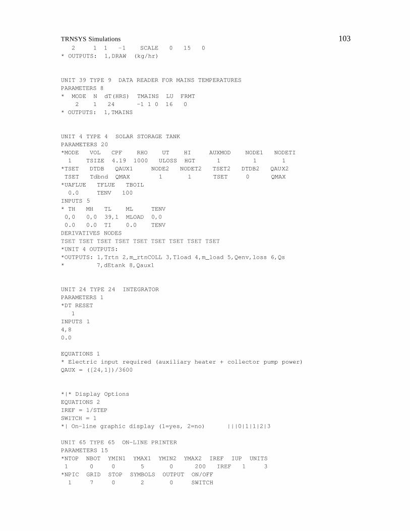
TRNSYS Simulations 103
2 1 1 -1 SCALE 0 15 0 * OUTPUTS: 1,DRAW (kg/hr) UNIT 39 TYPE 9 DATA READER FOR MAINS TEMPERATURES PARAMETERS 8 * MODE N dT(HRS) TMAINS LU FRMT 2 1 24 -1 1 0 16 0 * OUTPUTS: 1,TMAINS UNIT 4 TYPE 4 SOLAR STORAGE TANK PARAMETERS 20 *MODE VOL CPF RHO UT HI AUXMOD NODE1 NODETI 1 TSIZE 4.19 1000 ULOSS HGT 1 1 1 *TSET DTDB QAUX1 NODE2 NODET2 TSET2 DTDB2 QAUX2 TSET Tdbnd QMAX 1 1 TSET 0 QMAX *UAFLUE TFLUE TBOIL 0.0 TENV 100 INPUTS 5 * TH MH TL ML TENV 0,0 0,0 39,1 MLOAD 0,0 0.0 0.0 TI 0.0 TENV DERIVATIVES NODES TSET TSET TSET TSET TSET TSET TSET TSET TSET *UNIT 4 OUTPUTS: *OUTPUTS: 1,Trtn 2,m_rtnCOLL 3,Tload 4,m_load 5,Qenv,loss 6,Qs * 7,dEtank 8,Qaux1 UNIT 24 TYPE 24 INTEGRATOR PARAMETERS 1 *DT RESET 1 INPUTS 1 4,8 0.0 EQUATIONS 1 * Electric input required (auxiliary heater + collector pump power) QAUX = ([24,1])/3600 *|* Display Options EQUATIONS 2 IREF = 1/STEP SWITCH = 1 *| On-line graphic display (1=yes, 2=no) |||0|1|1|2|3 UNIT 65 TYPE 65 ON-LINE PRINTER PARAMETERS 15 *NTOP NBOT YMIN1 YMAX1 YMIN2 YMAX2 IREF IUP UNITS 1 0 0 5 0 200 IREF 1 3 *NPIC GRID STOP SYMBOLS OUTPUT ON/OFF 1 7 0 2 0 SWITCH

104 TRNSYS Simulations
INPUTS 1 QAUX Qaux LABELS 4 kWh kWh Average System Demand None UNIT 25 TYPE 25 PRINTER PARAMETERS 4 * DT TON TOFF LU 1 START STOP 10 INPUTS 1 QAUX ELCDMD UNIT 26 TYPE 25 plotter PARAMETERS 4 * DT TON TOFF LU 1 START STOP 17 INPUTS 1 QAUX ELCDMD END

TRNSYS Simulations 105
One Tank SDHW System
*TRNSED ASSIGN C:\ EUSESIA\ SYSTEMS\ SDHW1TNK.LST 6 ASSIGN C:\ EUSESIA\ SYSTEMS\ SDHW1TNK.OUT 10 ASSIGN C:\ EUSESIA\ SYSTEMS\ SDHW1TNK.PLT 22 ASSIGN C:\ EUSESIA\ SYSTEMS\ HRDRAW.DAT 15 ************************************************************** * This file predicts the required electric input to a solar * * domestic hot water system * ************************************************************** *|* Utility Location ASSIGN c:\ EUSESIA\ systems\ MLKWTR91.DAT 14 *|< City in which utility is located in |C:\ EUSESIA\ SYSTEMS\ CITIES.DAT|1|2|99 EQUATIONS 1 LAT = 4.2950E+0001 *|< City in which utility is located in |C:\ EUSESIA\ SYSTEMS\ CITIES.DAT|0|3|99 ASSIGN c:\ EUSESIA\ systems\ MLKMAIN.DAT 16 *|< City in which utility is located in |C:\ EUSESIA\ SYSTEMS\ CITIES.DAT|0|4|99 *|* *** SYSTEM PARAMETERS *** EQUATIONS 6 TSET = 60 TENV = 18 TI = 6.9 * * Determine the required draw from the tank. The following equations * account for the tempering valve. They result from simplified mass * and energy balances where Cp is assumed constant. TDIFF = MAX(0.000001,([4,3]-[39,1])) TNKDRW = MIN(1,((TSET-[39,1])/TDIFF)) MLOAD = [29,1]*TNKDRW * *** STANDARD ELECTRIC HOT WATER TANK *** * Volume: 80 gallon tank -> .3028 m3; * Height: 4.89 ft -> 1.4905 m * R-value: 16.7 (hr-ft2-F/Btu) -> ULOSS=1/R * .0489194(hr-m2-C/kJ)/(hr-ft2-F/Btu) *|* Tank Parameters EQUATIONS 7 TNKSIZE = 8.0000E+0001 *| Tank size |gal|gal|0|1|0|1000.00|3 TSIZE = .0037854*TNKSIZE HEIGHT1 = 4.8900E+0000
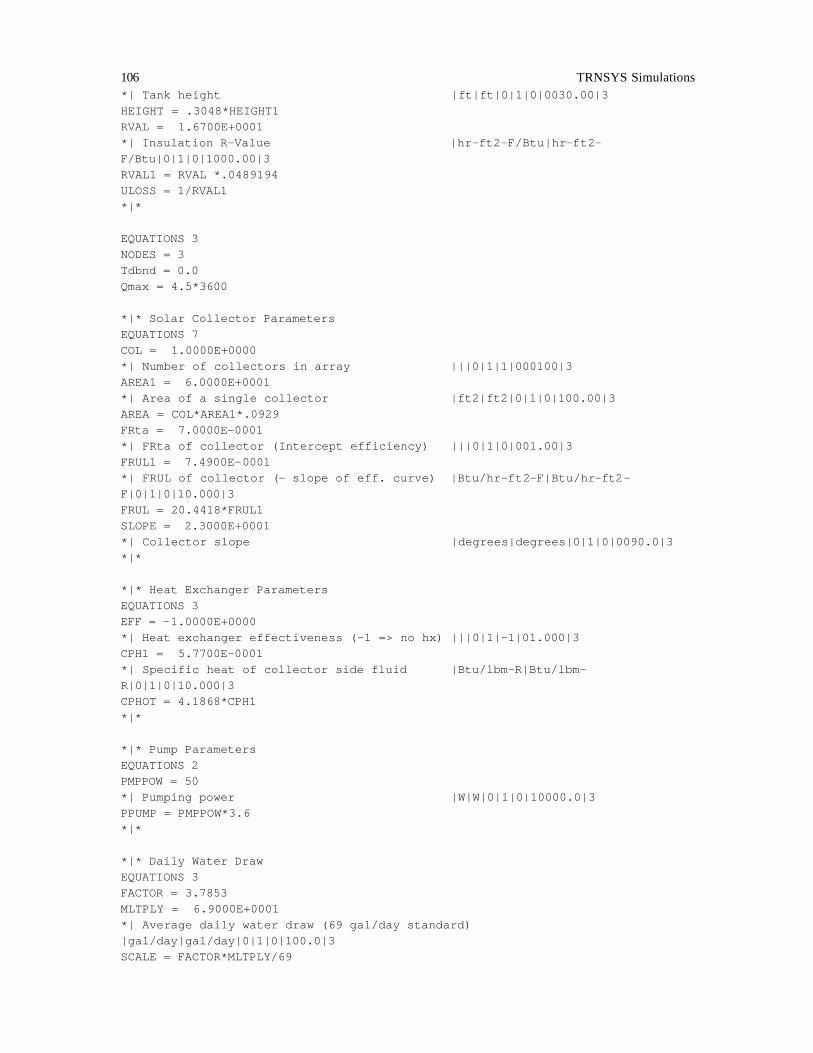
106 TRNSYS Simulations
*| Tank height |ft|ft|0|1|0|0030.00|3 HEIGHT = .3048*HEIGHT1 RVAL = 1.6700E+0001 *| Insulation R-Value |hr-ft2-F/Btu|hr-ft2-F/Btu|0|1|0|1000.00|3 RVAL1 = RVAL *.0489194 ULOSS = 1/RVAL1 *|* EQUATIONS 3 NODES = 3 Tdbnd = 0.0 Qmax = 4.5*3600 *|* Solar Collector Parameters EQUATIONS 7 COL = 1.0000E+0000 *| Number of collectors in array |||0|1|1|000100|3 AREA1 = 6.0000E+0001 *| Area of a single collector |ft2|ft2|0|1|0|100.00|3 AREA = COL*AREA1*.0929 FRta = 7.0000E-0001 *| FRta of collector (Intercept efficiency) |||0|1|0|001.00|3 FRUL1 = 7.4900E-0001 *| FRUL of collector (- slope of eff. curve) |Btu/hr-ft2-F|Btu/hr-ft2-F|0|1|0|10.000|3 FRUL = 20.4418*FRUL1 SLOPE = 2.3000E+0001 *| Collector slope |degrees|degrees|0|1|0|0090.0|3 *|* *|* Heat Exchanger Parameters EQUATIONS 3 EFF = -1.0000E+0000 *| Heat exchanger effectiveness (-1 => no hx) |||0|1|-1|01.000|3 CPH1 = 5.7700E-0001 *| Specific heat of collector side fluid |Btu/lbm-R|Btu/lbm-R|0|1|0|10.000|3 CPHOT = 4.1868*CPH1 *|* *|* Pump Parameters EQUATIONS 2 PMPPOW = 50 *| Pumping power |W|W|0|1|0|10000.0|3 PPUMP = PMPPOW*3.6 *|* *|* Daily Water Draw EQUATIONS 3 FACTOR = 3.7853 MLTPLY = 6.9000E+0001 *| Average daily water draw (69 gal/day standard) |gal/day|gal/day|0|1|0|100.0|3 SCALE = FACTOR*MLTPLY/69
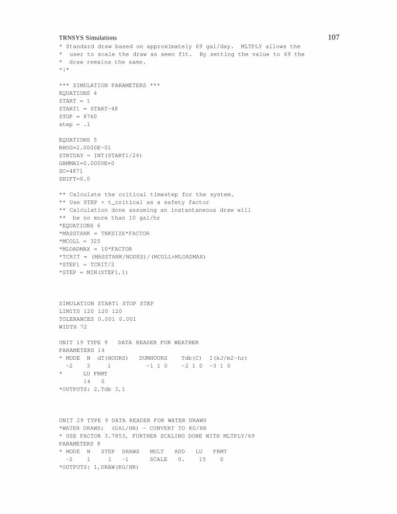
TRNSYS Simulations 107
* Standard draw based on approximately 69 gal/day. MLTPLY allows the * user to scale the draw as seen fit. By setting the value to 69 the * draw remains the same. *|* *** SIMULATION PARAMETERS *** EQUATIONS 4 START = 1 START1 = START-48 STOP = 8760 step = .1 EQUATIONS 5 RHOG=2.0000E-01 STRTDAY = INT(START1/24) GAMMAI=0.0000E+0 SC=4871 SHIFT=0.0 ** Calculate the critical timestep for the system. ** Use STEP < t_critical as a safety factor ** Calculation done assuming an instantaneous draw will ** be no more than 10 gal/hr *EQUATIONS 6 *MASSTANK = TNKSIZE*FACTOR *MCOLL = 325 *MLOADMAX = 10*FACTOR *TCRIT = (MASSTANK/NODES)/(MCOLL+MLOADMAX) *STEP1 = TCRIT/2 *STEP = MIN(STEP1,1) SIMULATION START1 STOP STEP LIMITS 120 120 120 TOLERANCES 0.001 0.001 WIDTH 72 UNIT 19 TYPE 9 DATA READER FOR WEATHER PARAMETERS 14 * MODE N dT(HOURS) DUMHOURS Tdb(C) I(kJ/m2-hr) -2 3 1 -1 1 0 -2 1 0 -3 1 0 * LU FRMT 14 0 *OUTPUTS: 2,Tdb 3,I UNIT 29 TYPE 9 DATA READER FOR WATER DRAWS *WATER DRAWS: (GAL/HR) - CONVERT TO KG/HR * USE FACTOR 3.7853, FURTHER SCALING DONE WITH MLTPLY/69 PARAMETERS 8 * MODE N STEP DRAWS MULT ADD LU FRMT -2 1 1 -1 SCALE 0. 15 0 *OUTPUTS: 1,DRAW(KG/HR)
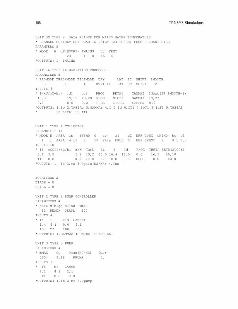
108 TRNSYS Simulations
UNIT 39 TYPE 9 DATA READER FOR MAINS WATER TEMPERATURE * CHANGES MONTHLY BUT READ IN DAILY (24 HOURS) FROM F-CHART FILE PARAMTERS 8 * MODE N dT(HOURS) TMAINS LU FRMT -2 1 24 -1 1 0 16 0 *OUTPUTS: 1, TMAINS UNIT 16 TYPE 16 RADIATION PROCESSOR PARAMETERS 8 * RADMODE TRACKMODE TILTMODE DAY LAT SC SHIFT SMOOTH 3 1 1 STRTDAY LAT SC SHIFT 2 INPUTS 6 * I(kJ/m2-hr) td1 td2 RHOG BETA1 GAMMAI INext(IF SMOOTH=1) 19,3 19,19 19,20 RHOG SLOPE GAMMAI 19,23 0.0 0.0 0.0 RHOG SLOPE GAMMAI 0.0 *OUTPUTS: 1,Io 2,THETAz 3,GAMMAs 4,I 5,Id 6,IT1 7,IbT1 8,IdT1 9,THETA1 * 10,BETA1 11,IT1 UNIT 1 TYPE 1 COLLECTOR PARAMETERS 14 * MODE N AREA Cp EFFMD G ao a1 a2 EFF CpHX OPTMD bo b1 1 1 AREA 4.19 1 50 FRta FRUL 0. EFF CPHOT 1 0.1 0.0 INPUTS 10 * Ti mCOLL(kg/hr) mHX Tamb It I Id RHOG THETA BETA(SLOPE) 3,1 3,2 3,2 19,2 16,6 16,4 16,5 0,0 16,9 16,10 TI 0.0 0.0 20.0 0.0 0.0 0.0 RHOG 0.0 40.0 *OUPUTS: 1, To 2,mo 3,Qgain(KJ/HR) 4,Tco EQUATIONS 2 DEADH = 0 DEADL = 0 UNIT 2 TYPE 2 PUMP CONTROLLER PARAMETERS 4 * NSTK dThigh dTlow Tmax 11 DEADH DEADL 100 INPUTS 4 * Th Tl TIN GAMMAI 1,4 4,1 0,0 2,1 15. TI 100 0. *OUTPUTS: 1,GAMMAo (CONTROL FUNCTION) UNIT 3 TYPE 3 PUMP PARAMETERS 4 * mMAX Cp Pmax(KJ/HR) fpar 325. 4.19 PPUMP 0. INPUTS 3 * Ti mi GAMMA 4,1 4,2 2,1 TI 0.0 0.0 *OUTPUTS: 1,To 2,mo 3,Ppump

TRNSYS Simulations 109
EQUATIONS 1 HGT = -HEIGHT UNIT 4 TYPE 4 SOLAR STORAGE TANK PARAMETERS 20 *MODE VOL CPF RHO UT HI AUXMOD NODE1 NODETI 2 TSIZE 4.19 1000 ULOSS HGT 1 1 1 *TSET DTDB QAUX1 NODE2 NODET2 TSET2 DTDB2 QAUX2 TSET 0 QMAX 1 1 TSET 0 0.0 *UAFLUE TFLUE TBOIL 0.0 TENV 100 INPUTS 5 * TH MH TL ML TENV 1,1 1,2 39,1 MLOAD 0,0 0.0 0.0 TI 0.0 TENV DERIVATIVES NODES TSET TSET TSET TSET TSET TSET TSET TSET TSET *UNIT 4 OUTPUTS: *OUTPUTS: 1,Trtn 2,m_rtnCOLL 3,Tload 4,m_load 5,Qenv,loss 6,Qs * 7,dEtank 8,Qaux1 UNIT 24 TYPE 24 INTEGRATOR PARAMETERS 1 *DT RESET 1 INPUTS 2 4,8 3,3 0.0 0.0 EQUATIONS 2 * Electric input required (auxiliary heater + collector pump power) ELECDMND = ([24,1]+[24,2])/3600 QAUX = ([24,1])/3600 UNIT 25 TYPE 25 PRINTER PARAMETERS 4 * DT TON TOFF LU 1 START STOP 10 INPUTS 1 elecdmnd elcdmd UNIT 26 TYPE 25 plotting PRINTER PARAMETERS 4 * DT TON TOFF LU 1 START STOP 22 INPUTS 1 elecdmnd elcdmd *|* Display Options

110 TRNSYS Simulations
EQUATIONS 2 IREF = 1/(STEP+.00001) SWITCH = 1.0000E+0000 *| On-line graphic display (1=yes, 2=no) |||0|1|1|2|3 UNIT 65 TYPE 65 ON-LINE PRINTER PARAMETERS 15 *NTOP NBOT YMIN1 YMAX1 YMIN2 YMAX2 IREF IUP UNITS 2 1 0 5 0 80 IREF 1 3 *NPIC GRID STOP SYMBOLS OUTPUT ON/OFF 1 7 0 2 0 SWITCH INPUTS 3 QAUX ELECDMND MLOAD Qaux ElecDmnd MTANK LABELS 4 kW kg/hr Average System Demand Tank Draw END

TRNSYS Simulations 111
Two Tank SDHW System
*TRNSED ASSIGN C:\ EUSESIA\ SYSTEMS\ SDHW2TNK.LST 6 ASSIGN C:\ EUSESIA\ SYSTEMS\ SDHW2TNK.OUT 10 ASSIGN C:\ EUSESIA\ SYSTEMS\ SDHW2TNK.PLT 22 ASSIGN C:\ EUSESIA\ SYSTEMS\ HRDRAW.DAT 15 ***************************************************************** * This file predicts the required electric input to a two tank * * solar domestic hot water system * ***************************************************************** *|* Utility Location ASSIGN c:\ EUSESIA\ systems\ MLKWTR91.DAT 14 *|< City in which utility is located in |C:\ EUSESIA\ SYSTEMS\ CITIES.DAT|1|2|99 EQUATIONS 1 LAT = 4.2950E+0001 *|< City in which utility is located in |C:\ EUSESIA\ SYSTEMS\ CITIES.DAT|0|3|99 ASSIGN c:\ EUSESIA\ systems\ MLKMAIN.DAT 16 *|< City in which utility is located in |C:\ EUSESIA\ SYSTEMS\ CITIES.DAT|0|4|99 *|* *** SYSTEM PARAMETERS *** EQUATIONS 6 TSET = 60 TENV = 18 TI = 6.9 * * Determine the required draw from the tank. The following equations * account for the tempering valve. They result from simplified mass * and energy balances where Cp is assumed constant. TDIFF = MAX(0.000001,([4,3]-[39,1])) TNKDRW = MIN(1,((TSET-[39,1])/TDIFF)) MLOAD = [29,1]*TNKDRW * *** STANDARD ELECTRIC HOT WATER TANK *** * Volume: 80 gallon tank -> .3028 m3; * Height: 4.89 ft -> 1.4905 m * R-value: 16.7 (hr-ft2-F/Btu) -> ULOSS=1/R * .0489194(hr-m2-C/kJ)/(hr-ft2-F/Btu) *|* Solar Storage Tank Parameters EQUATIONS 7 TNKSIZES = 8.0000E+0001 *| Tank size |gal|gal|0|1|0|1000.00|3 TSIZES = .0037854*TNKSIZES HEIGHT1S = 4.8900E+0000

112 TRNSYS Simulations
*| Tank height |ft|ft|0|1|0|0030.00|3 HEIGHTS = .3048*HEIGHT1S RVALS = 1.6700E+0001 *| Insulation R-Value |hr-ft2-F/Btu|hr-ft2-F/Btu|0|1|0|1000.00|3 RVALS1 = RVALS *.0489194 ULOSSS = 1/RVALS1 *|* *|* Auxiliary Tank Parameters EQUATIONS 7 TNKSIZEA = 8.0000E+0001 *| Tank size |gal|gal|0|1|0|1000.00|3 TSIZEA = .0037854*TNKSIZEA HEIGHT1A = 4.8900E+0000 *| Tank height |ft|ft|0|1|0|0030.00|3 HEIGHTA = .3048*HEIGHT1A RVALA = 1.6700E+0001 *| Insulation R-Value |hr-ft2-F/Btu|hr-ft2-F/Btu|0|1|0|1000.00|3 RVALA1 = RVALA *.0489194 ULOSSA = 1/RVALA1 *|* ** Other tank parameters. S -> solar, A -> auxiliary EQUATIONS 4 NODES = 3 NODEA = 3 Tdbnd = 0.0 Qmax = 4.5*3600 *|* Solar Collector Parameters EQUATIONS 7 COL = 1.0000E+0000 *| Number of collectors in array |||0|1|0|000100|3 AREA1 = 6.0000E+0001 *| Area of a single collector |ft2|ft2|0|1|0|100.00|3 AREA = AREA1*.0929 FRta = 7.0000E-0001 *| FRta of collector (Intercept efficiency) |||0|1|0|001.00|3 FRUL1 = 7.4900E-0001 *| FRUL of collector (- slope of eff. curve) |Btu/hr-ft2-F|Btu/hr-ft2-F|0|1|0|10.000|3 FRUL = 20.4418*FRUL1 SLOPE= 2.3000E+0001 *| Collector slope |degrees|degrees|0|1|0|0090.0|3 *|* *|* Heat Exchanger Parameters EQUATIONS 3 EFF = -1.0000E+0000 *| Heat exchanger effectiveness (-1 => no hx) |||0|1|-1|01.000|3 CPH1 = 5.7700E-0001 *| Specific heat of collector side fluid |Btu/lbm-R|Btu/lbm-R|0|1|0|10.000|3
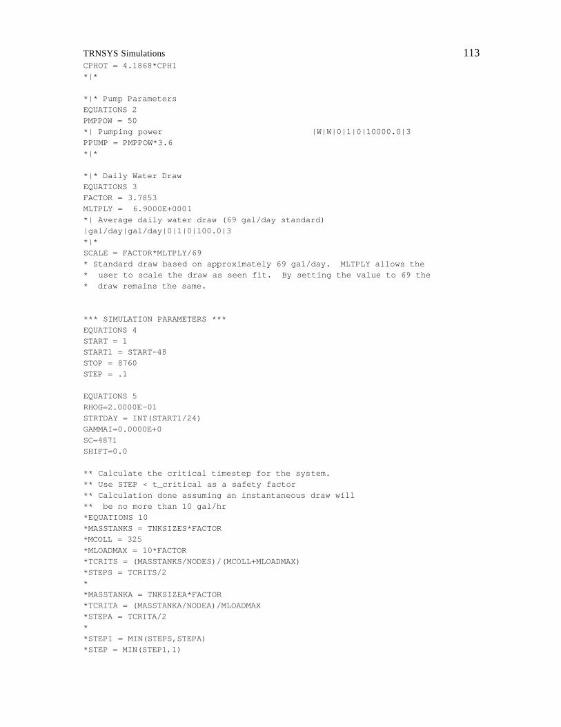
TRNSYS Simulations 113
CPHOT = 4.1868*CPH1 *|* *|* Pump Parameters EQUATIONS 2 PMPPOW = 50 *| Pumping power |W|W|0|1|0|10000.0|3 PPUMP = PMPPOW*3.6 *|* *|* Daily Water Draw EQUATIONS 3 FACTOR = 3.7853 MLTPLY = 6.9000E+0001 *| Average daily water draw (69 gal/day standard) |gal/day|gal/day|0|1|0|100.0|3 *|* SCALE = FACTOR*MLTPLY/69 * Standard draw based on approximately 69 gal/day. MLTPLY allows the * user to scale the draw as seen fit. By setting the value to 69 the * draw remains the same. *** SIMULATION PARAMETERS *** EQUATIONS 4 START = 1 START1 = START-48 STOP = 8760 STEP = .1 EQUATIONS 5 RHOG=2.0000E-01 STRTDAY = INT(START1/24) GAMMAI=0.0000E+0 SC=4871 SHIFT=0.0 ** Calculate the critical timestep for the system. ** Use STEP < t_critical as a safety factor ** Calculation done assuming an instantaneous draw will ** be no more than 10 gal/hr *EQUATIONS 10 *MASSTANKS = TNKSIZES*FACTOR *MCOLL = 325 *MLOADMAX = 10*FACTOR *TCRITS = (MASSTANKS/NODES)/(MCOLL+MLOADMAX) *STEPS = TCRITS/2 * *MASSTANKA = TNKSIZEA*FACTOR *TCRITA = (MASSTANKA/NODEA)/MLOADMAX *STEPA = TCRITA/2 * *STEP1 = MIN(STEPS,STEPA) *STEP = MIN(STEP1,1)
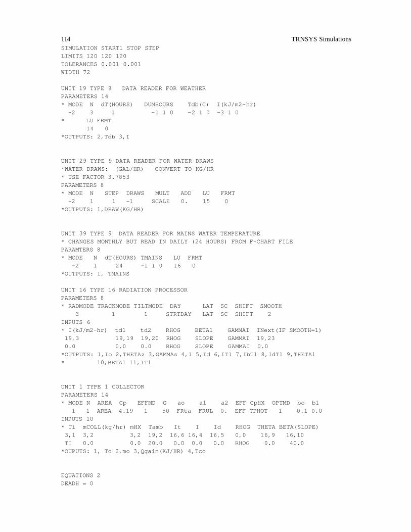
114 TRNSYS Simulations
SIMULATION START1 STOP STEP LIMITS 120 120 120 TOLERANCES 0.001 0.001 WIDTH 72 UNIT 19 TYPE 9 DATA READER FOR WEATHER PARAMETERS 14 * MODE N dT(HOURS) DUMHOURS Tdb(C) I(kJ/m2-hr) -2 3 1 -1 1 0 -2 1 0 -3 1 0 * LU FRMT 14 0 *OUTPUTS: 2,Tdb 3,I UNIT 29 TYPE 9 DATA READER FOR WATER DRAWS *WATER DRAWS: (GAL/HR) - CONVERT TO KG/HR * USE FACTOR 3.7853 PARAMETERS 8 * MODE N STEP DRAWS MULT ADD LU FRMT -2 1 1 -1 SCALE 0. 15 0 *OUTPUTS: 1,DRAW(KG/HR) UNIT 39 TYPE 9 DATA READER FOR MAINS WATER TEMPERATURE * CHANGES MONTHLY BUT READ IN DAILY (24 HOURS) FROM F-CHART FILE PARAMTERS 8 * MODE N dT(HOURS) TMAINS LU FRMT -2 1 24 -1 1 0 16 0 *OUTPUTS: 1, TMAINS UNIT 16 TYPE 16 RADIATION PROCESSOR PARAMETERS 8 * RADMODE TRACKMODE TILTMODE DAY LAT SC SHIFT SMOOTH 3 1 1 STRTDAY LAT SC SHIFT 2 INPUTS 6 * I(kJ/m2-hr) td1 td2 RHOG BETA1 GAMMAI INext(IF SMOOTH=1) 19,3 19,19 19,20 RHOG SLOPE GAMMAI 19,23 0.0 0.0 0.0 RHOG SLOPE GAMMAI 0.0 *OUTPUTS: 1,Io 2,THETAz 3,GAMMAs 4,I 5,Id 6,IT1 7,IbT1 8,IdT1 9,THETA1 * 10,BETA1 11,IT1 UNIT 1 TYPE 1 COLLECTOR PARAMETERS 14 * MODE N AREA Cp EFFMD G ao a1 a2 EFF CpHX OPTMD bo b1 1 1 AREA 4.19 1 50 FRta FRUL 0. EFF CPHOT 1 0.1 0.0 INPUTS 10 * Ti mCOLL(kg/hr) mHX Tamb It I Id RHOG THETA BETA(SLOPE) 3,1 3,2 3,2 19,2 16,6 16,4 16,5 0,0 16,9 16,10 TI 0.0 0.0 20.0 0.0 0.0 0.0 RHOG 0.0 40.0 *OUPUTS: 1, To 2,mo 3,Qgain(KJ/HR) 4,Tco EQUATIONS 2 DEADH = 0

TRNSYS Simulations 115
DEADL = 0 UNIT 2 TYPE 2 PUMP CONTROLLER PARAMETERS 4 * NSTK dThigh dTlow Tmax 11 DEADH DEADL 100 INPUTS 4 * Th Tl TIN GAMMAI 1,4 5,1 0,0 2,1 15. TI 100 0. *OUTPUTS: 1,GAMMAo (CONTROL FUNCTION) UNIT 3 TYPE 3 PUMP PARAMETERS 4 * mMAX Cp Pmax(KJ/HR) fpar 325. 4.19 PPUMP 0. INPUTS 3 * Ti mi GAMMA 5,1 5,2 2,1 TI 0.0 0.0 *OUTPUTS: 1,To 2,mo 3,Ppump EQUATIONS 2 HGTA = -HEIGHTA HGTS = -HEIGHTS UNIT 5 TYPE 4 SOLAR STORAGE TANK PARAMETERS 20 *MODE VOL CPF RHO UT HI AUXMOD NODE1 NODETI 2 TSIZES 4.19 1000 ULOSSS HGTS 1 1 1 *TSET DTDB QAUX1 NODE2 NODET2 TSET2 DTDB2 QAUX2 TSET 0 0.0 1 1 TSET 0 0.0 *UAFLUE TFLUE TBOIL 0.0 TENV 100 INPUTS 5 * TH MH TL ML TENV 1,1 1,2 39,1 MLOAD 0,0 0.0 0.0 TI 0.0 TENV DERIVATIVES NODES TSET TSET TSET TSET TSET TSET TSET TSET TSET *OUTPUTS: 1,Trtn 2,m_rtnCOLL 3,Tload 4,m_load 5,Qenv,loss 6,Qs * 7,dEtank 8,Qaux1 UNIT 4 TYPE 4 AUXILIARY TANK PARAMETERS 20 *MODE VOL CPF RHO UT HI AUXMOD NODE1 NODETI 2 TSIZEA 4.19 1000 ULOSSA HGTA 1 1 1 *TSET DTDB QAUX1 NODE2 NODET2 TSET2 DTDB2 QAUX2 TSET 0 QMAX 1 1 TSET 0 0.0 *UAFLUE TFLUE TBOIL 0.0 TENV 100 INPUTS 5 * TH MH TL ML TENV 0,0 0,0 5,3 5,4 0,0

116 TRNSYS Simulations
0.0 0.0 TI 0.0 TENV DERIVATIVES NODEA TSET TSET TSET TSET TSET TSET TSET *UNIT 4 OUTPUTS: *OUTPUTS: 1,Trtn 2,m_rtnCOLL 3,Tload 4,m_load 5,Qenv,loss 6,Qs * 7,dEtank 8,Qaux1 UNIT 24 TYPE 24 INTEGRATOR PARAMETERS 1 *DT RESET 1 INPUTS 2 4,8 3,3 0.0 0.0 EQUATIONS 2 * Electric input required (auxiliary heater + collector pump power) ELECDMND = ([24,1]+[24,2])/3600 QAUX = ([24,1])/3600 UNIT 25 TYPE 25 PRINTER PARAMETERS 4 * DT TON TOFF LU 1 START STOP 10 INPUTS 1 elecdmnd elcdmd UNIT 26 TYPE 25 plotting PRINTER PARAMETERS 4 * DT TON TOFF LU 1 START STOP 22 INPUTS 1 elecdmnd elcdmd *|* Display Options EQUATIONS 2 IREF = 1/STEP SWITCH = 1.0000E+0000 *| On-line graphic display (1=yes, 2=no) |||0|1|1|2|3 UNIT 65 TYPE 65 ON-LINE PRINTER PARAMETERS 15 *NTOP NBOT YMIN1 YMAX1 YMIN2 YMAX2 IREF IUP UNITS 2 1 0 5 0 80 IREF 1 3 *NPIC GRID STOP SYMBOLS OUTPUT ON/OFF 1 7 0 2 0 SWITCH INPUTS 3 QAUX ELECDMND MLOAD Qaux ElecDmnd MTANK LABELS 4 kW kg/hr

TRNSYS Simulations 117
Average System Demand Tank Draw END

118 TRNSYS Simulations
One Tank System with SRCC Collector *TRNSED ASSIGN C:\ EUSESIA\ SYSTEMS\ SRCC1TNK.LST 6 ASSIGN C:\ EUSESIA\ SYSTEMS\ SRCC1TNK.OUT 10 ASSIGN C:\ EUSESIA\ SYSTEMS\ SRCC1TNK.PLT 22 ASSIGN C:\ EUSESIA\ SYSTEMS\ HRDRAW.DAT 15 ************************************************************** * This file predicts the required electric input to a solar * * domestic hot water system * ************************************************************** *|* Utility Location ASSIGN c:\ EUSESIA\ systems\ MLKWTR91.DAT 14 *|< City in which utility is located in |C:\ EUSESIA\ SYSTEMS\ CITIES.DAT|1|2|99 EQUATIONS 1 LAT = 4.2950E+0001 *|< City in which utility is located in |C:\ EUSESIA\ SYSTEMS\ CITIES.DAT|0|3|99 ASSIGN c:\ EUSESIA\ systems\ MLKMAIN.DAT 16 *|< City in which utility is located in |C:\ EUSESIA\ SYSTEMS\ CITIES.DAT|0|4|99 *|* *** SYSTEM PARAMETERS *** EQUATIONS 6 TSET = 60 TENV = 18 TI = 6.9 * * Determine the required draw from the tank. The following equations * account for the tempering valve. They result from simplified mass * and energy balances where Cp is assumed constant. TDIFF = MAX(0.000001,([4,3]-[39,1])) TNKDRW = MIN(1,((TSET-[39,1])/TDIFF)) MLOAD = [29,1]*TNKDRW * *** STANDARD ELECTRIC HOT WATER TANK *** * Volume: 80 gallon tank -> .3028 m3; * Height: 4.89 ft -> 1.4905 m * R-value: 16.7 (hr-ft2-F/Btu) -> ULOSS=1/R * .0489194(hr-m2-C/kJ)/(hr-ft2-F/Btu) *|* Tank Parameters EQUATIONS 7 TNKSIZE = 8.0000E+0001 *| Tank size |gal|gal|0|1|0|1000.00|3 TSIZE = .0037854*TNKSIZE HEIGHT1 = 4.8900E+0000

TRNSYS Simulations 119
*| Tank height |ft|ft|0|1|0|0030.00|3 HEIGHT = .3048*HEIGHT1 RVAL = 1.6700E+0001 *| Insulation R-Value |hr-ft2-F/Btu|hr-ft2-F/Btu|0|1|0|1000.00|3 RVAL1 = RVAL *.0489194 ULOSS = 1/RVAL1 *|* EQUATIONS 3 NODES = 3 Tdbnd = 0.0 Qmax = 4.5*3600 *|* SRCC Rated Solar Collector Parameters EQUATIONS 9 AREA1 = 2.9100E+0001 *|< SRCC rated collector |C:\ EUSESIA\ SYSTEMS\ SRCC.DAT|1|2|99 AREA = AREA1*.0929 FRta = 8.7100E-0001 *|< FRta of collector (Intercept efficiency) |C:\ EUSESIA\ SYSTEMS\ SRCC.DAT|0|3|99 FRUL1 = 3.7350E+0000 *|< FRUL of collector (- slope of eff. curve) |C:\ EUSESIA\ SYSTEMS\ SRCC.DAT|0|4|99 FRUL = 20.4418*FRUL1 B0 = 3.1600E-0002 *|< 1st order inc ang modifier coeff (-S) |C:\ EUSESIA\ SYSTEMS\ SRCC.DAT|0|5|99 B1 = 1.0400E-0002 *|< 2nd order inc ang modifier coeff (-S2) |C:\ EUSESIA\ SYSTEMS\ SRCC.DAT|0|6|99 COL = 1.0000E+0000 *| Number of collectors in array |||0|1|0|000100|3 SLOPE= 2.3000E+0001 *| Collector slope |degrees|degrees|0|1|0|0090.0|3 *|* *|* Heat Exchanger Parameters EQUATIONS 3 EFF = -1.0000E+0000 *| Heat exchanger effectiveness (-1 => no hx) |||0|1|-1|01.000|3 CPH1 = 5.7700E-0001 *| Specific heat of collector side fluid |Btu/lbm-R|Btu/lbm-R|0|1|0|10.000|3 CPHOT = 4.1868*CPH1 *|* *|* Pump Parameters EQUATIONS 2 PMPPOW = 50 *| Pumping power |W|W|0|1|0|10000.0|3 PPUMP = PMPPOW*3.6 *|*

120 TRNSYS Simulations
*|* Daily Water Draw EQUATIONS 3 FACTOR = 3.7853 MLTPLY = 6.9000E+0001 *| Average daily water draw (69 gal/day standard) |gal/day|gal/day|0|1|0|100.0|3 *|* SCALE = FACTOR*MLTPLY/69 * Standard draw based on approximately 69 gal/day. MLTPLY allows the * user to scale the draw as seen fit. By setting the value to 69 the * draw remains the same. *** SIMULATION PARAMETERS *** EQUATIONS 4 START = 1 START1 = START-48 STOP = 8760 STEP = .1 EQUATIONS 5 RHOG=2.0000E-01 STRTDAY = INT(START1/24) GAMMAI=0.0000E+0 SC=4871 SHIFT=0.0 ** Calculate the critical timestep for the system. ** Use STEP < t_critical as a safety factor ** Calculation done assuming an instantaneous draw will ** be no more than 10 gal/hr *EQUATIONS 6 *MASSTANK = TNKSIZE*FACTOR *MCOLL = 325 *MLOADMAX = 10*FACTOR *TCRIT = (MASSTANK/NODES)/(MCOLL+MLOADMAX) *STEP1 = TCRIT/2 *STEP = MIN(STEP1,1) SIMULATION START1 STOP STEP LIMITS 120 120 120 TOLERANCES 0.001 0.001 WIDTH 72 UNIT 19 TYPE 9 DATA READER FOR WEATHER PARAMETERS 14 * MODE N dT(HOURS) DUMHOURS Tdb(C) I(kJ/m2-hr) -2 3 1 -1 1 0 -2 1 0 -3 1 0 * LU FRMT 14 0 *OUTPUTS: 2,Tdb 3,I UNIT 29 TYPE 9 DATA READER FOR WATER DRAWS *WATER DRAWS: (GAL/HR) - CONVERT TO KG/HR

TRNSYS Simulations 121
* USE FACTOR 3.7853 PARAMETERS 8 * MODE N STEP DRAWS MULT ADD LU FRMT -2 1 1 -1 SCALE 0. 15 0 *OUTPUTS: 1,DRAW(KG/HR) UNIT 39 TYPE 9 DATA READER FOR MAINS WATER TEMPERATURE * CHANGES MONTHLY BUT READ IN DAILY (24 HOURS) FROM F-CHART FILE PARAMTERS 8 * MODE N dT(HOURS) TMAINS LU FRMT -2 1 24 -1 1 0 16 0 *OUTPUTS: 1, TMAINS UNIT 16 TYPE 16 RADIATION PROCESSOR PARAMETERS 8 * RADMODE TRACKMODE TILTMODE DAY LAT SC SHIFT SMOOTH 3 1 1 STRTDAY LAT SC SHIFT 2 INPUTS 6 * I(kJ/m2-hr) td1 td2 RHOG BETA1 GAMMAI INext(IF SMOOTH=1) 19,3 19,19 19,20 RHOG SLOPE GAMMAI 19,23 0.0 0.0 0.0 RHOG SLOPE GAMMAI 0.0 *OUTPUTS: 1,Io 2,THETAz 3,GAMMAs 4,I 5,Id 6,IT1 7,IbT1 8,IdT1 9,THETA1 * 10,BETA1 11,IT1 UNIT 1 TYPE 1 COLLECTOR PARAMETERS 14 * MODE N AREA Cp EFFMD G ao a1 a2 EFF CpHX OPTMD bo b1 1 1 AREA 4.19 1 50 FRta FRUL 0. EFF CPHOT 1 B0 B1 INPUTS 10 * Ti mCOLL(kg/hr) mHX Tamb It I Id RHOG THETA BETA(SLOPE) 3,1 3,2 3,2 19,2 16,6 16,4 16,5 0,0 16,9 16,10 TI 0.0 0.0 20.0 0.0 0.0 0.0 RHOG 0.0 40.0 *OUPUTS: 1, To 2,mo 3,Qgain(KJ/HR) 4,Tco EQUATIONS 2 DEADH = 0 DEADL = 0 UNIT 2 TYPE 2 PUMP CONTROLLER PARAMETERS 4 * NSTK dThigh dTlow Tmax 11 DEADH DEADL 100 INPUTS 4 * Th Tl TIN GAMMAI 1,4 4,1 0,0 2,1 15. TI 100 0. *OUTPUTS: 1,GAMMAo (CONTROL FUNCTION) UNIT 3 TYPE 3 PUMP PARAMETERS 4 * mMAX Cp Pmax(KJ/HR) fpar 325. 4.19 PPUMP 0.

122 TRNSYS Simulations
INPUTS 3 * Ti mi GAMMA 4,1 4,2 2,1 TI 0.0 0.0 *OUTPUTS: 1,To 2,mo 3,Ppump EQUATIONS 1 HGT = -HEIGHT UNIT 4 TYPE 4 SOLAR STORAGE TANK PARAMETERS 20 *MODE VOL CPF RHO UT HI AUXMOD NODE1 NODETI 2 TSIZE 4.19 1000 ULOSS HGT 1 1 1 *TSET DTDB QAUX1 NODE2 NODET2 TSET2 DTDB2 QAUX2 TSET 0 QMAX 1 1 TSET 0 0.0 *UAFLUE TFLUE TBOIL 0.0 TENV 100 INPUTS 5 * TH MH TL ML TENV 1,1 1,2 39,1 MLOAD 0,0 0.0 0.0 TI 0.0 TENV DERIVATIVES NODES TSET TSET TSET TSET TSET TSET TSET TSET TSET *UNIT 4 OUTPUTS: *OUTPUTS: 1,Trtn 2,m_rtnCOLL 3,Tload 4,m_load 5,Qenv,loss 6,Qs * 7,dEtank 8,Qaux1 UNIT 24 TYPE 24 INTEGRATOR PARAMETERS 1 *DT RESET 1 INPUTS 2 4,8 3,3 0.0 0.0 EQUATIONS 2 * Electric input required (auxiliary heater + collector pump power) ELECDMND = ([24,1]+[24,2])/3600 QAUX = ([24,1])/3600 UNIT 25 TYPE 25 PRINTER PARAMETERS 4 * DT TON TOFF LU 1 START STOP 10 INPUTS 1 elecdmnd elcdmd UNIT 26 TYPE 25 plotting PRINTER PARAMETERS 4 * DT TON TOFF LU 1 START STOP 22

TRNSYS Simulations 123
INPUTS 1 elecdmnd elcdmd *|* Display Options EQUATIONS 2 IREF = 1/STEP SWITCH = 1.0000E+0000 *| On-line graphic display (1=yes, 2=no) |||0|1|1|2|3 UNIT 65 TYPE 65 ON-LINE PRINTER PARAMETERS 15 *NTOP NBOT YMIN1 YMAX1 YMIN2 YMAX2 IREF IUP UNITS 2 1 0 5 0 80 IREF 1 3 *NPIC GRID STOP SYMBOLS OUTPUT ON/OFF 1 7 0 2 0 SWITCH INPUTS 3 QAUX ELECDMND MLOAD Qaux ElecDmnd MTANK LABELS 4 kW kg/hr Average System Demand Tank Draw END

124 TRNSYS Simulations
Two Tank System with SRCC Collector *TRNSED ASSIGN C:\ EUSESIA\ SYSTEMS\ SRCC2TNK.LST 6 ASSIGN C:\ EUSESIA\ SYSTEMS\ SRCC2TNK.OUT 10 ASSIGN C:\ EUSESIA\ SYSTEMS\ SRCC2TNK.PLT 22 ASSIGN C:\ EUSESIA\ SYSTEMS\ HRDRAW.DAT 15 ************************************************************** * This file predicts the required electric input to a solar * * domestic hot water system * ************************************************************** *|* Utility Location ASSIGN c:\ EUSESIA\ systems\ MLKWTR91.DAT 14 *|< City in which utility is located in |C:\ EUSESIA\ SYSTEMS\ CITIES.DAT|1|2|99 EQUATIONS 1 LAT = 4.2950E+0001 *|< City in which utility is located in |C:\ EUSESIA\ SYSTEMS\ CITIES.DAT|0|3|99 ASSIGN c:\ EUSESIA\ systems\ MLKMAIN.DAT 16 *|< City in which utility is located in |C:\ EUSESIA\ SYSTEMS\ CITIES.DAT|0|4|99 *|* *** SYSTEM PARAMETERS *** EQUATIONS 6 TSET = 60 TENV = 18 TI = 6.9 * * Determine the required draw from the tank. The following equations * account for the tempering valve. They result from simplified mass * and energy balances where Cp is assumed constant. TDIFF = MAX(0.000001,([4,3]-[39,1])) TNKDRW = MIN(1,((TSET-[39,1])/TDIFF)) MLOAD = [29,1]*TNKDRW * *** STANDARD ELECTRIC HOT WATER TANK *** * Volume: 80 gallon tank -> .3028 m3; * Height: 4.89 ft -> 1.4905 m * R-value: 16.7 (hr-ft2-F/Btu) -> ULOSS=1/R * .0489194(hr-m2-C/kJ)/(hr-ft2-F/Btu) *|* Solar Storage Tank Parameters EQUATIONS 7 TNKSIZES = 8.0000E+0001 *| Tank size |gal|gal|0|1|0|1000.00|3 TSIZES = .0037854*TNKSIZES HEIGHT1S = 4.8900E+0000

TRNSYS Simulations 125
*| Tank height |ft|ft|0|1|0|0030.00|3 HEIGHTS = .3048*HEIGHT1S RVALS = 1.6700E+0001 *| Insulation R-Value |hr-ft2-F/Btu|hr-ft2-F/Btu|0|1|0|1000.00|3 RVALS1 = RVALS *.0489194 ULOSSS = 1/RVALS1 *|* *|* Auxiliary Tank Parameters EQUATIONS 7 TNKSIZEA = 8.0000E+0001 *| Tank size |gal|gal|0|1|0|1000.00|3 TSIZEA = .0037854*TNKSIZEA HEIGHT1A = 4.8900E+0000 *| Tank height |ft|ft|0|1|0|0030.00|3 HEIGHTA = .3048*HEIGHT1A RVALA = 1.6700E+0001 *| Insulation R-Value |hr-ft2-F/Btu|hr-ft2-F/Btu|0|1|0|1000.00|3 RVALA1 = RVALA *.0489194 ULOSSA = 1/RVALA1 *|* ** Other tank parameters. S -> solar, A -> auxiliary EQUATIONS 4 NODES = 3 NODEA = 3 Tdbnd = 0.0 Qmax = 4.5*3600 *|* SRCC Rated Solar Collector Parameters EQUATIONS 9 AREA1 = 2.9100E+0001 *|< SRCC rated collector |C:\ EUSESIA\ SYSTEMS\ SRCC.DAT|1|2|99 AREA = AREA1*.0929 FRta = 8.7100E-0001 *|< FRta of collector (Intercept efficiency) |C:\ EUSESIA\ SYSTEMS\ SRCC.DAT|0|3|99 FRUL1 = 3.7350E+0000 *|< FRUL of collector (- slope of eff. curve |C:\ EUSESIA\ SYSTEMS\ SRCC.DAT|0|4|99 FRUL = 20.4418*FRUL1 B0 = .0316 *|< 1st order inc ang modifier coeff (-S) |C:\ EUSESIA\ SYSTEMS\ SRCC.DAT|0|5|99 B1 = .0104 *|< 2nd order inc ang modifier coeff (-S2) |C:\ EUSESIA\ SYSTEMS\ SRCC.DAT|0|6|99 COL = 1.0000E+0000 *| Number of collectors in array |||0|1|0|000100|3 SLOPE= 2.3000E+0001 *| Collector slope |degrees|degrees|0|1|0|0090.0|3 *|*

126 TRNSYS Simulations
*|* Heat Exchanger Parameters EQUATIONS 3 EFF = -1.0000E+0000 *| Heat exchanger effectiveness (-1 => no hx) |||0|1|-1|01.000|3 CPH1 = 5.7700E-0001 *| Specific heat of collector side fluid |Btu/lbm-R|Btu/lbm-R|0|1|0|10.000|3 CPHOT = 4.1868*CPH1 *|* *|* Pump Parameters EQUATIONS 2 PMPPOW = 50 *| Pumping power |W|W|0|1|0|10000.0|3 PPUMP = PMPPOW*3.6 *|* *|* Daily Water Draw EQUATIONS 3 FACTOR = 3.7853 MLTPLY = 6.9000E+0001 *| Average daily water draw (69 gal/day standard) |gal/day|gal/day|0|1|0|100.0|3 *|* SCALE = FACTOR*MLTPLY/69 * Standard draw based on approximately 69 gal/day. MLTPLY allows the * user to scale the draw as seen fit. By setting the value to 69 the * draw remains the same. EQUATIONS 4 *** SIMULATION PARAMETERS *** START = 1 START1 = START-48 STOP = 8760 STEP = .1 EQUATIONS 5 RHOG=2.0000E-01 STRTDAY = INT(START1/24) GAMMAI=0.0000E+0 SC=4871 SHIFT=0.0 ** Calculate the critical timestep for the system. ** Use STEP < t_critical as a safety factor ** Calculation done assuming an instantaneous draw will ** be no more than 10 gal/hr *EQUATIONS 10 *MASSTANKS = TNKSIZES*FACTOR *MCOLL = 325 *MLOADMAX = 10*FACTOR *TCRITS = (MASSTANKS/NODES)/(MCOLL+MLOADMAX)

TRNSYS Simulations 127
*STEPS = TCRITS/2 * *MASSTANKA = TNKSIZEA*FACTOR *TCRITA = (MASSTANKA/NODEA)/MLOADMAX *STEPA = TCRITA/2 * *STEP1 = MIN(STEPS,STEPA) *STEP = MIN(STEP1,1) SIMULATION START1 STOP STEP LIMITS 120 120 120 TOLERANCES 0.001 0.001 WIDTH 72 UNIT 19 TYPE 9 DATA READER FOR WEATHER PARAMETERS 14 * MODE N dT(HOURS) DUMHOURS Tdb(C) I(kJ/m2-hr) -2 3 1 -1 1 0 -2 1 0 -3 1 0 * LU FRMT 14 0 *OUTPUTS: 2,Tdb 3,I UNIT 29 TYPE 9 DATA READER FOR WATER DRAWS *WATER DRAWS: (GAL/HR) - CONVERT TO KG/HR * USE FACTOR 3.7853 PARAMETERS 8 * MODE N STEP DRAWS MULT ADD LU FRMT -2 1 1 -1 SCALE 0. 15 0 *OUTPUTS: 1,DRAW(KG/HR) UNIT 39 TYPE 9 DATA READER FOR MAINS WATER TEMPERATURE * CHANGES MONTHLY BUT READ IN DAILY (24 HOURS) FROM F-CHART FILE PARAMTERS 8 * MODE N dT(HOURS) TMAINS LU FRMT -2 1 24 -1 1 0 16 0 *OUTPUTS: 1, TMAINS UNIT 16 TYPE 16 RADIATION PROCESSOR PARAMETERS 8 * RADMODE TRACKMODE TILTMODE DAY LAT SC SHIFT SMOOTH 3 1 1 STRTDAY LAT SC SHIFT 2 INPUTS 6 * I(kJ/m2-hr) td1 td2 RHOG BETA1 GAMMAI INext(IF SMOOTH=1) 19,3 19,19 19,20 RHOG SLOPE GAMMAI 19,23 0.0 0.0 0.0 RHOG SLOPE GAMMAI 0.0 *OUTPUTS: 1,Io 2,THETAz 3,GAMMAs 4,I 5,Id 6,IT1 7,IbT1 8,IdT1 9,THETA1 * 10,BETA1 11,IT1 UNIT 1 TYPE 1 COLLECTOR PARAMETERS 14 * MODE N AREA Cp EFFMD G ao a1 a2 EFF CpHX OPTMD bo b1

128 TRNSYS Simulations
1 1 AREA 4.19 1 50 FRta FRUL 0. EFF CPHOT 1 B0 B1 INPUTS 10 * Ti mCOLL(kg/hr) mHX Tamb It I Id RHOG THETA BETA(SLOPE) 3,1 3,2 3,2 19,2 16,6 16,4 16,5 0,0 16,9 16,10 TI 0.0 0.0 20.0 0.0 0.0 0.0 RHOG 0.0 40.0 *OUPUTS: 1, To 2,mo 3,Qgain(KJ/HR) 4,Tco EQUATIONS 2 DEADH = 0 DEADL = 0 UNIT 2 TYPE 2 PUMP CONTROLLER PARAMETERS 4 * NSTK dThigh dTlow Tmax 11 DEADH DEADL 100 INPUTS 4 * Th Tl TIN GAMMAI 1,4 5,1 0,0 2,1 15. TI 100 0. *OUTPUTS: 1,GAMMAo (CONTROL FUNCTION) UNIT 3 TYPE 3 PUMP PARAMETERS 4 * mMAX Cp Pmax(KJ/HR) fpar 325. 4.19 PPUMP 0. INPUTS 3 * Ti mi GAMMA 5,1 5,2 2,1 TI 0.0 0.0 *OUTPUTS: 1,To 2,mo 3,Ppump EQUATIONS 2 HGTA = -HEIGHTA HGTS = -HEIGHTS UNIT 5 TYPE 4 SOLAR STORAGE TANK PARAMETERS 20 *MODE VOL CPF RHO UT HI AUXMOD NODE1 NODETI 2 TSIZES 4.19 1000 ULOSSS HGTS 1 1 1 *TSET DTDB QAUX1 NODE2 NODET2 TSET2 DTDB2 QAUX2 TSET 0 0.0 1 1 TSET 0 0.0 *UAFLUE TFLUE TBOIL 0.0 TENV 100 INPUTS 5 * TH MH TL ML TENV 1,1 1,2 39,1 MLOAD 0,0 0.0 0.0 TI 0.0 TENV DERIVATIVES NODES TSET TSET TSET TSET TSET TSET TSET TSET TSET *OUTPUTS: 1,Trtn 2,m_rtnCOLL 3,Tload 4,m_load 5,Qenv,loss 6,Qs * 7,dEtank 8,Qaux1 UNIT 4 TYPE 4 AUXILIARY TANK PARAMETERS 20
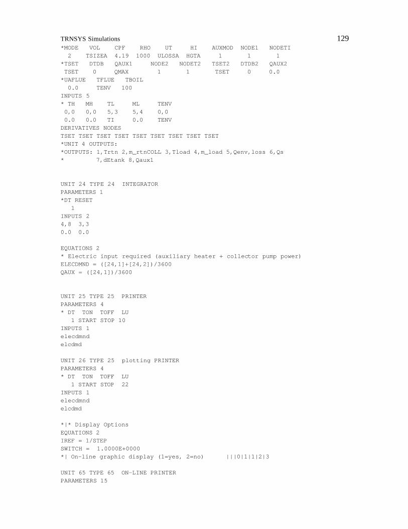
TRNSYS Simulations 129
*MODE VOL CPF RHO UT HI AUXMOD NODE1 NODETI 2 TSIZEA 4.19 1000 ULOSSA HGTA 1 1 1 *TSET DTDB QAUX1 NODE2 NODET2 TSET2 DTDB2 QAUX2 TSET 0 QMAX 1 1 TSET 0 0.0 *UAFLUE TFLUE TBOIL 0.0 TENV 100 INPUTS 5 * TH MH TL ML TENV 0,0 0,0 5,3 5,4 0,0 0.0 0.0 TI 0.0 TENV DERIVATIVES NODES TSET TSET TSET TSET TSET TSET TSET TSET TSET *UNIT 4 OUTPUTS: *OUTPUTS: 1,Trtn 2,m_rtnCOLL 3,Tload 4,m_load 5,Qenv,loss 6,Qs * 7,dEtank 8,Qaux1 UNIT 24 TYPE 24 INTEGRATOR PARAMETERS 1 *DT RESET 1 INPUTS 2 4,8 3,3 0.0 0.0 EQUATIONS 2 * Electric input required (auxiliary heater + collector pump power) ELECDMND = ([24,1]+[24,2])/3600 QAUX = ([24,1])/3600 UNIT 25 TYPE 25 PRINTER PARAMETERS 4 * DT TON TOFF LU 1 START STOP 10 INPUTS 1 elecdmnd elcdmd UNIT 26 TYPE 25 plotting PRINTER PARAMETERS 4 * DT TON TOFF LU 1 START STOP 22 INPUTS 1 elecdmnd elcdmd *|* Display Options EQUATIONS 2 IREF = 1/STEP SWITCH = 1.0000E+0000 *| On-line graphic display (1=yes, 2=no) |||0|1|1|2|3 UNIT 65 TYPE 65 ON-LINE PRINTER PARAMETERS 15

130 TRNSYS Simulations
*NTOP NBOT YMIN1 YMAX1 YMIN2 YMAX2 IREF IUP UNITS 2 1 0 5 0 80 IREF 1 3 *NPIC GRID STOP SYMBOLS OUTPUT ON/OFF 1 7 0 2 0 SWITCH INPUTS 3 QAUX ELECDMND MLOAD Qaux ElecDmnd MTANK LABELS 4 kW kg/hr Average System Demand Tank Draw END

TRNSYS Simulations 131
Photovoltaic System *TRNSED ASSIGN C:\ EUSESIA\ SYSTEMS\ PV1.LST 6 ASSIGN C:\ EUSESIA\ SYSTEMS\ PV1.OUT 10 ASSIGN C:\ EUSESIA\ SYSTEMS\ PV1.PLT 22 ************************************************************** * This file predicts the required electric input to a solar * * photovoltaic system * ************************************************************** *|* Utility Location ASSIGN c:\ EUSESIA\ systems\ MLKWTR91.DAT 14 *|< City in which utility is located |c:\ EUSESIA\ systems\ cities.dat|1|2|99 EQUATIONS 1 LAT = 4.2950E+0001 *|< City in which utility is located |c:\ EUSESIA\ systems\ cities.dat|0|3|99 *|* EQUATIONS 4 RHOG = .2 SC = 4871 SHIFT = 0 GAMMAI = 0 EQUATIONS 5 START = 1 STOP = 8760 STEP = 1 START1 = START-48 STRTDAY =INT(START1/24) SIMULATION START1 STOP STEP LIMITS 120 120 120 TOLERANCES 0.001 0.001 WIDTH 72 Equations 22 *|* Photovoltaic Panels SunRef= 1.0000E+0003 *|< Photovoltaic panel selection |c:\ EUSESIA\ systems\ PVMODUL2.DAT|1|2|0 Tcref = 2.9800E+0002 *|<Photovoltaic panel selection |c:\ EUSESIA\ systems\ PVMODUL2.DAT|0|3|0 Iscref = 1.8000E+0000 *|<Photovoltaic panel selection |c:\ EUSESIA\ systems\ PVMODUL2.DAT|0|4|0 Vocref = 5.5500E+0001

132 TRNSYS Simulations
*|<Photovoltaic panel selection |c:\ EUSESIA\ systems\ PVMODUL2.DAT|0|5|0 Imref = 1.3200E+0000 *|<Photovoltaic panel selection |c:\ EUSESIA\ systems\ PVMODUL2.DAT|0|6|0 Vmref= 3.8000E+0001 *|<Photovoltaic panel selection |c:\ EUSESIA\ systems\ PVMODUL2.DAT|0|7|0 Misc = 1.5000E-0003 *|<Photovoltaic panel selection |c:\ EUSESIA\ systems\ PVMODUL2.DAT|0|8|0 Mvoc = -1.9425E-0001 *|<Photovoltaic panel selection |c:\ EUSESIA\ systems\ PVMODUL2.DAT|0|9|0 tau_alfa = 9.0000E-0001 *|<Photovoltaic panel selection |c:\ EUSESIA\ systems\ PVMODUL2.DAT|0|10|0 E_q = 1.1550E+0000 *|<Photovoltaic panel selection |c:\ EUSESIA\ systems\ PVMODUL2.DAT|0|11|0 NCS= 6.6000E+0001 *|<Photovoltaic panel selection |c:\ EUSESIA\ systems\ PVMODUL2.DAT|0|12|0 width = 8.0000E-0001 *|<Photovoltaic panel selection |c:\ EUSESIA\ systems\ PVMODUL2.DAT|0|13|0 length = 1.5250E+0000 *|<Photovoltaic panel selection |c:\ EUSESIA\ systems\ PVMODUL2.DAT|0|14|0 Ns_pv = 6.0000E+0000 *| Number of panels in series |||0|1|1|1000|0 Np_pv = 1.0000E+0000 *| Number of panels in parallel |||0|1|1|1000|0 Mode_pv = 2.0000E+0000 MPPT_Eff = 9.5000E-0001 *| Eff. of the max. power point tracker |||0|1|0|1.00|0 DINRG = 100 U_L = 10 SLOPE= 2.3000E+0001 *| Slope of collector |Degrees||0|1|-180.00|180.00|0 *|* *|* DC/AC Inverter Invr_Eff = 9.5000E-0001 *| Inverter efficiency |||0|1|0|1.00|0 V_grid = 1.1000E+0002 *| Grid operating voltage |Volts||0|1|100|250.|0 ********************************************************* UNIT 19 TYPE 9 DATA READER FOR WEATHER PARAMETERS 14 * MODE N dT(HOURS) DUMHOURS Tdb(C) I(kJ/m2-hr) -2 3 1 -1 1 0 -2 1 0 -3 1 0 * LU FRMT 14 0 *OUTPUTS: 2,Tdb 3,I ********************************************************* UNIT 16 TYPE 16 Radiation Processor PARAMETERS 8 *RADMODE TRACKMODE TILTMODE DAY LAT SC SHIFT SMOOTH 3 1 1 STRTDAY LAT SC SHIFT 2 INPUTS 6 *I(kJ/hr-m2) td1 td2 RHOG BETA1 GAMMAI INEXT(IF SMOOTH=1) 19,3 19,19 19,20 RHOG SLOPE GAMMAI 19,23

TRNSYS Simulations 133
0.0 0.0 1.0 RHOG SLOPE GAMMAI 0.0 *OUTPUTS: 1)Io 2)THETAz 3)GAMMAs 4)I 5)Id 6)IT1 7)IbT1 * 8)IdT1 9)THETA1 10)BETA1 11)IT1 ********************************************************* EQUATION 2 solar = [16,6]/3.6 T_amb = [19,2] ********************************************************* unit 62 type 62 PV array * PV paramters Parameters 9 Mode_pv Sunref Tcref Iscref Vocref Imref Vmref Misc Mvoc Parameters 8 tau_alfa E_q NCS width length Ns_pv Np_pv DINRG Inputs 3 *Sun Tamb U_L 16,6 T_amb U_L 3600 25.0 10.0 ********************************************************* unit 70 type 70 DC/DC + DC/AC Parameter 1 3 Inputs 5 * Imp Vmp V_grid Eta_DC_DC Eta_DC_AC 62,4 62,5 0,0 0,0 0,0 2. 50. V_grid MPPT_Eff Invr_Eff ********************************************************* Equation 1 Qsolar = solar * width * length * Ns_pv * Np_pv ********************************************************* unit 23 type 24 Quantity Integrator, Hourly Parameters 1 *Dt 1 inputs 2 *Qsolar Qelec Qsolar 70,3 10000 100.

134 TRNSYS Simulations
********************************************************* Equations 2 Qsol_k = [23,1] / 1000 Qelc_k = [23,2] / 1000 ********************************************************* UNIT 26 TYPE 25 PRINTER PARAMETERS 4 1 start STOP 10 INPUTS 1 *Qelec Qelc_k ElcDmd ********************************************************* Equation 1 Ymax1 = Int((width * length * Np_pv * Ns_pv)/5 + 0.9) * 5000 ********************************************************* *|* *|* Display Options EQUATIONS 1 SWITCH = 1.0000E+0000 *| On-line graphic display (1=yes, 2=no) |||0|1|1|2|3 unit 65 type 65 ONLINE GRAPHICS PARAMETERS 15 *Ntop Nbot Ymin,1 Ymax,1 Ymin,2 Ymax,2 1 0 0.0 5.0 -25. 100. *Iref Iupd units Npic Grid Stop Symbols Outputs 1 1 3 1 7 0 2 0 *Plot (Yes/No) SWITCH inputs 1 Qelc_k Electrical labels 4 kW none Average System Generation ********************************************************* END

TRNSYS Simulations 135
Marginal Plant Prediction *TRNSED ASSIGN \ EUSESIA\ UTILMIX\ MARPLANT.LST 6 ASSIGN \ EUSESIA\ utilmix\ marplant.plt 10 ******************************* ****** FRONT END ****** ******************************* *|* Prediction of the Marginal Plant *|* for a Specified Region of Utilities *|* *|* *** Assign the plant data file and the load file *** *|* Utility Region to be Analyzed ASSIGN c:\ EUSESIA\ utilmix\ WEPCO.DAT 15 *|< Utility region |C:\ EUSESIA\ UTILMIX\ REGIONS.DAT|1|2|0 ASSIGN c:\ EUSESIA\ utilmix\ WEPCO.LOD 16 *|< Utility region |C:\ EUSESIA\ UTILMIX\ REGIONS.DAT|0|3|0 ASSIGN c:\ EUSESIA\ utilmix\ WEPCO.PRF 14 *|< Utility region |C:\ EUSESIA\ UTILMIX\ REGIONS.DAT|0|4|0 EQUATIONS 1 LIMIT = 8000 *| Estimate region capacity |MW|MW|0|1|0|100000||0 EQUATIONS 3 START = 1 STOP = 8760 STEP = 1 SIMULATION START STOP STEP TOLERANCES .001 .001 ****************************** ****** DATA READERS ****** ****************************** UNIT 11 TYPE 99 LOAD PROFILE DATA READER PARAMETERS 11 * MODE NUMVALS DT LOAD * + EUE * + LU FRMT -2 2 1 -1 1 0 -2 1 0 16 0 *OUTPUTS: 1)LOAD 2)MARGINAL EUE *********************************** ****** FIND PLANT PROFILE ****** *********************************** UNIT 72 TYPE 72 MARGINAL PLANT PREDICTOR PARAMETERS 1 *LU 15 INPUTS 2

136 TRNSYS Simulations
*LOAD MAREUE 11,1 11,2 1.0 0.0 *OUTPUTS: 1)LOAD 2)MARGINAL PLANT 3)MAGINAL EUE 4)MARGINAL OPERATING COST * 5)TOTAL ADJUSTED CAPACITY ************************************ ****** OUTPUT AND DISPLAY ****** ************************************ UNIT 25 TYPE 25 PRINTER PARAMETERS 4 * DT T_ON T_OFF LU UNITS 1 START STOP 14 0 INPUTS 5 *LOAD MARPLANT MAREUE MARCOST TOTCAP 72,1 72,2 72,3 72,4 72,5 LOAD MARPLANT MAREUE MARCOST TOTCAP *OUTPUTS: 1)LOAD 2)MARPLANT 3)MAREUE 4)MARCOST 5)TOTCAP UNIT 26 TYPE 25 plotting PRINTER PARAMETERS 4 * DT T_ON T_OFF LU UNITS 1 START STOP 10 0 INPUTS 4 *LOAD MAREUE MARCOST TOTAL ADJUSTED CAPACITY 72,1 72,3 72,4 72,5 LOAD MAREUE MARCST CAPACITY *OUTPUTS: 1)LOAD 2)MAREUE 3)MARCOST 4)CAPACITY UNIT 65 TYPE 65 ON-LINE PRINTER PARAMETERS 15 * #_TOP #_BOT YMN1 YMX1 YMN2 YMX2 IREF IUP UNITS NPIC GRID STOP SYM OUT ON/OFF 2 1 0 LIMIT 0 .25 1 1 3 1 7 1 2 0 1 INPUTS 3 * LOAD CAPACITY MARCOST 11,1 72,5 72,4 LOAD CAP MARCST LABELS 4 MW $ Utility Load Marginal Operating Cost END

TRNSYS Simulations 137
Utility Impact Analysis *TRNSED ASSIGN C:\ EUSESIA\ UTILITY.LST 6 ASSIGN C:\ EUSESIA\ UTILITY.PLT 11 ASSIGN C:\ EUSESIA\ UTIL1.DAT 15 ASSIGN C:\ EUSESIA\ UTIL2.DAT 16 ASSIGN C:\ EUSESIA\ UTIL3.DAT 17 ASSIGN C:\ EUSESIA\ UTIL4.DAT 18 ASSIGN C:\ EUSESIA\ UTIL5.DAT 19 ASSIGN C:\ EUSESIA\ UTIL6.DAT 20 ASSIGN C:\ EUSESIA\ UTIL7.DAT 28 ******************************* ****** FRONT END ****** ******************************* *|* Electric Utility Solar Energy System Impact Analysis: *|* *|* Economic and Environmental Benefits from a Large Scale *|* Implementation of Solar Energy Systems *|* *|* *|* Date: |10/95 *|* Organization: |SEL *|* Input prepared by: |Trzesniewski *|* *|* *|* Utility Information ASSIGN c:\ EUSESIA\ utilmix\ WEPCO.LOD 12 *|< Utility to be analyzed |C:\ EUSESIA\ UTILMIX\ LOADS.DAT|1|2|0 ASSIGN c:\ EUSESIA\ utilmix\ WISCRGN.PRF 14 *|< Utility region to be analyzed |C:\ EUSESIA\ UTILMIX\ REGIONS.DAT|1|4|0 ASSIGN c:\ EUSESIA\ utilmix\ WISCRGN.DAT 13 *|< Utility region to be analyzed |C:\ EUSESIA\ UTILMIX\ REGIONS.DAT|0|2|0 EQUATIONS 1 LIMIT = 2.0000E+0004 *| Estimate region capacity |MW|MW|0|1|0|100000|0 *|* EQUATIONS 5 CUSTOMERS = 1.0000E+0005 *| Number of electric customers |||0|1|0|100000000|0 TRNLSS = 2.0000E+0000 *| System transmission losses |%|%|0|1|0|000100.00|0 DISLSS = 3.0000E+0000 *| System distribution losses |%|%|0|1|0|000100.00|0 TRNSLOSS = TRNLSS/100 DISTLOSS = DISLSS/100 *|* *|* Solar Energy System ASSIGN c:\ EUSESIA\ systems\ mlk1tnk.out 22 *|< Solar system |C:\ EUSESIA\ SYSTEMS\ SOLSYS.DAT|1|2|0 EQUATIONS 9

138 TRNSYS Simulations
SOLMODE = 1.0000E+0000 *|< Solar system |C:\ EUSESIA\ SYSTEMS\ SOLSYS.DAT|0|3|0 SYSCOST = 2.0000E+0003 *| Installed cost of solar system |$/unit|$/unit|0|1|0|100000|0 ACCEPT = 5.0000E+0000 *| % of customers accepting program |%|%|0|1|0|0100.0|0 DOWNPAY = 1.4000E+0002 *| Customer down payment on system |$|$|0|1|0|001000|0 LEAS = 1.2000E+0001 *| Customer monthly lease payment |$/mo|$/mo|0|1|0|100.00|0 LEASE = LEAS*12 OANDM = 1.0000E+0001 *| Operation and maintenance |$/yr-system|$/yr-system|0|1|0|001000|0 DEPYRS = 5.0000E+0000 *| Equipment depreciation period |yrs|yrs|0|1|0|000100|0 NUMSYS = CUSTOMERS*ACCEPT/100 *|* *|* Comparative System ASSIGN c:\ EUSESIA\ systems\ mlkedhw.out 21 *|< Electric system |C:\ EUSESIA\ SYSTEMS\ ELECSYS.DAT|1|2|0 *|* *|* Emission Costs EQUATIONS 8 CO2 = 0.0000E+0000 *| CO2 |$/lbm|$/ton|0|2000|0|10000.0000|0 SO2 = 2.0000E-0002 *| SO2 |$/lbm|$/ton|0|2000|0|10000.0000|0 NOX = 0.0000E+0000 *| NOX |$/lbm|$/ton|0|2000|0|10000.0000|0 N2O = 0.0000E+0000 *| N2O |$/lbm|$/ton|0|2000|0|10000.0000|0 PARTS = 0.0000E+0000 *| Particulates |$/lbm|$/ton|0|2000|0|10000.0000|0 CH4 = 0.0000E+0000 *| CH4 |$/lbm|$/ton|0|2000|0|10000.0000|0 MERCURY = 0.0000E+0000 *| Mercury |$/lbm|$/ton|0|2000|0|10000.0000|0 NUKES = 0.0000E+0000 *| Nuclear waste |$/lbm|$/ton|0|2000|0|10000.0000|0 *|* *|* Demand Reduction Parameters EQUATIONS 8 RESRVMARGN= 1.5000E+0001 *| Reserve margin |%|%|0|1|0|000100.00|0 RESRVMAR = RESRVMARGN/100 DMNDWORTH = 2.5000E+0002 *| Cost of conventional option per kW |$/kW|$/kW|0|1|0|100000.00|0 TRNSWORTH = 1.0000E+0002 *| Cost of adding kW of transmission capacity |$/kW|$/kW|0|1|0|100000.00|0 DISTWORTH = 1.0000E+0002 *| Cost of adding kW of distribution capacity |$/kW|$/kW|0|1|0|100000.00|0 DMODE = 2.0000E+0000

TRNSYS Simulations 139
*|< Demand evaluation method |C:\ EUSESIA\ METHOD.DAT|1|2|0 PEAKS = 2.0000E+0001 *| Number of peak hours to evaluate |||0|1|0|000000100|0 CCIREF = 9.2000E-0001 *| CCI of conventional reference option |||0|1|0|0001.0000|0 *|* *|* Electric Customer Retention EQUATIONS 3 NOPROGLOSS= 4.0000E+0000 *| % customers lost to other fuel w/o program |%|%|0|1|0|00100|0 PROGLOSS = 2.0000E+0000 *| % customers lost to other fuel with program |%|%|0|1|0|00100|0 RETAINWRTH= 0.0000E+0000 *| Value of retained customer |$/yr|$/yr|0|1|0|10000|0 *|* *|* Delayed Power Plant Construction CONSTANTS 1 DELAYWORTH= 0.0000E+0000 *| Value of delaying power plant construction |$/peak kW|$/peak kW|0|1|0|100000|0 *|* *|* Government Incentives for Investment CONSTANTS 3 TAXCRD = 1.0000E+0001 *| Tax credit given for investment |%|%|0|1|0|0100.00|0 TAXCREDIT = TAXCRD/100 SUBSIDY = 1.5000E-0002 *| Energy subsidy |$/kWh|$/kWh|0|1|0|100.000|0 *|* *|* Economic Parameters CONSTANTS 7 NUMYRS = 2.0000E+0001 *| Years of economic analysis |yrs|yrs|0|1|1|000100|0 IRATE = 5.0000E+0000 *| Inflation rate |%|%|0|1|0|100.00|0 INFRATE = IRATE/100 DRATE = 8.0000E+0000 *| Discount rate |%|%|0|1|0|100.00|0 DISRATE = DRATE/100 TAXBR = 3.4000E+0001 *| Utility tax bracket |%|%|0|1|0|100.00|0 TAXBRACK = TAXBR/100 *|* *|* Customer Rate Information EQUATIONS 2 WINRATE = 6.4000E-0002 *| Winter rate |$/kWh|$/kWh|0|1|0|1.0000|0 SUMRATE = 7.4500E-0002 *| Summer rate |$/kWh|$/kWh|0|1|0|1.0000|0

140 TRNSYS Simulations
EQUATIONS 3 START = 1 STOP = 8760 STEP = 1 SIMULATION START STOP STEP TOLERANCES .001 .001 WIDTH 132 ****************************** ****** DATA READERS ****** ****************************** UNIT 9 TYPE 99 EDHW SYSTEM OUTPUT DATA READER PARAMETERS 11 * MODE NUMVALS DT HR * + ELECDMND * + LU FRMT -2 2 1 -1 1 0 -2 1 0 21 0 *OUTPUTS: 2)ELECDMND UNIT 10 TYPE 99 SDHW SYSTEM OUTPUT DATA READER PARAMETERS 11 * MODE NUMVALS DT HR * + SOLDMND * + LU FRMT -2 2 1 -1 1 0 -2 1 0 22 0 *OUTPUTS: 2)SOLDMND UNIT 11 TYPE 99 REGIONAL LOAD PROFILE DATA READER PARAMETERS 17 * MODE NUMVALS DT HR * + LOAD * + PLANT * + MAREUE * + -2 4 1 -1 1 0 -2 1 0 -3 1 0 -4 1 0 * LU FRMT 14 0 *OUTPUTS: 2)LOAD 3)MARGINAL PLANT 4)MARGIANL EUE UNIT 12 TYPE 99 UTILITY LOAD PROFILE DATA READER PARAMETERS 8 * MODE NUMVALS DT LOAD * + LU FRMT -2 1 1 -1 1 0 12 0 *OUTPUTS: 1)LOAD ********************************* *** SINGLE SYSTEM PERFORMANCE *** ********************************* EQUATIONS 2 ELECDMND = [9,2] SOLDMND = [10,2] UNIT 30 TYPE 24 MONTHLY INTEGRATOR PARAMETERS 1 *DTRESET -1 INPUTS 2 *ELECDMND SOLDMND ELECDMND SOLDMND 1. 1.

TRNSYS Simulations 141
EQUATIONS 2 SOLMNTH = [30,2] ELCMNTH = [30,1] *************************** ****** ECONOMICS ****** *************************** UNIT 71 TYPE 71 UTILITY ENERGY & ECONOMIC IMPACT ANALYSIS PARAMETERS 20 * #SYSTS CO2 SO2 NOX N2O PARTS CH4 MERCURY NUKES NUMSYS CO2 SO2 NOX N2O PARTS CH4 MERCURY NUKES * RESERVE MARGIN DMNDWORTH TRNSWORTH DISTWORTH DMODE PEAKS RESRVMAR DMNDWORTH TRNSWORTH DISTWORTH DMODE PEAKS * REFERENECE CCI TRNSLOSS DISTLOSS SOLMODE LU CCIREF TRNSLOSS DISTLOSS SOLMODE 13 INPUTS 5 * ELECDMND SOLDMMD LOAD MARPLANT MAREUE ELECDMND SOLDMND 11,2 11,3 11,4 0.0 0.0 0.0 0.0 0.0 *OUTPUTS: 1)ENERGY RED(kWh) 2)ENERGY SAVINGS($) 3)CO2 RED(lbm) 4)CO2 SAVINGS($) * 5)SO2 RED(lbm) 6)SO2 SAVINGS($) 7)NOX RED(lbm) 8)NOX SAVINGS($) * 9)N2O RED(lbm) 10)N2O SAVINGS($) 11)PARTS RED(lbm) 12)PARTS SAVINGS($) * 13)CH4 RED(lbm) 14)CH4 SAVINGS($) 15)HG RED(lbm) 16)HG SAVINGS($) * 17)NUKE RED(lbm) 18)NUKE SAVINGS($) 19)POLLUTION SAVINGS($) * 20)DEMAND REDUCTION(kW) 21)DEMAND SAVINGS($) * 22)DEMAND REDUCTION AT PEAK LOAD(kW) 23)OPTION CCI UNIT 72 TYPE 24 INTEGRATOR INPUTS 10 * kWh ENERGY $ ENERGY LBMCO2 $CO2 LBMSO2 $SO2 LBMNOX $NOX 71,1 71,2 71,3 71,4 71,5 71,6 71,7 71,8 * LBMN2O $N2O 71,9 71,10 0 0 0 0 0 0 0 0 0 0 UNIT 73 TYPE 24 INTEGRATOR INPUTS 9 * LBMPARTS $PARTS LBMCH4 $CH4 LBMHG $HG LBMNUKE $NUKE 71,11 71,12 71,13 71,14 71,15 71,16 71,17 71,18 * $POLLUTION 71,19 0 0 0 0 0 0 0 0 0 0 *** PRE-ECONOMIC SUMMARY EQUATIONS *** EQUATIONS 3 DELAYVAL = DELAYWORTH * [71,22] RETAINVAL = RETAINWRTH*CUSTOMERS*(NOPROGLOSS-PROGLOSS)/100 SUBSDYCRDT = SUBSIDY * [72,1] UNIT 74 TYPE 89 UTILITY ECONOMIC SUMMARY

142 TRNSYS Simulations
PARAMETERS 12 * LIFE YRS INFLATION DISCOUNT #SYSTS $/SYSTEM DOWN PAYMENT NUMYRS INFRATE DISRATE NUMSYS SYSCOST DOWNPAY * LEASE OANDM RETENTION VALUE TAX BRACKET DEPYRS TAX CREDIT LEASE OANDM RETAINVAL TAXBRACK DEPYRS TAXCREDIT INPUTS 5 * $ENERGY $DEMAND $POLLUTION DELAY VALUE SUBSIDY CREDIT 72,2 71,21 73,9 DELAYVAL SUBSDYCRDT 0.0 0.0 0.0 0.0 0.0 *OUTPUTS: 1)PRESENT WORTH OF INVESTMENT 2)LEVELIZED COST 3)RATE OF RETURN * 4)DEMAND SAVINGS AFTER 1ST YEAR 5)PW INVESTMENT 6)PW DELAY VALUE * 7)PW RETENTION 8)PW DOWNPAYMENTS 9)PW TAX CREDIT 10)PW DEMAND SAV * 11)PW ENERGY SAV 12)PW EMISSION SAV 13)PW SUBSIDY 14)PW O&M * 15)PW DEPRECIATION 16)PW LEASE ************************************ ****** OUTPUT AND DISPLAY ****** ************************************ UNIT 25 TYPE 25 OUTPUT PRINTER PARAMETERS 4 * DT T_ON T_OFF LU UNITS 1 STOP STOP 15 1 INPUTS 10 * kWh ENERGY $ ENERGY LBMCO2 $CO2 LBMSO2 $SO2 LBMNOX $NOX 72,1 72,2 72,3 72,4 72,5 72,6 72,7 72,8 * LBMN2O $N2O 72,9 72,10 ENRED ENSAV LBMCO2 $CO2 LBMSO2 $SO2 LBMNOX $NOX LBMN2O $N2O UNIT 26 TYPE 25 OUTPUT PRINTER PARAMETERS 4 * DT T_ON T_OFF LU UNITS 1 STOP STOP 16 1 INPUTS 10 * LBMPARTS $PARTS LBMCH4 $CH4 LBMHG $HG LBMNUKE $NUKE 73,1 73,2 73,3 73,4 73,5 73,6 73,7 73,8 * $POLLUTION NUMSYS 73,9 NUMSYS LBMPARTS $PARTS LBMCH4 $CH4 LBMHG $HG LBMNUKE $NUKE $POLLUTION NUMSYS UNIT 27 TYPE 25 OUTPUT PRINTER PARAMETERS 4 * DT T_ON T_OFF LU UNITS 1 STOP STOP 17 1 INPUTS 10 * DMNDRED DMNDSAV CCI PRESWORTH LEVELCOST ROR 71,20 74,4 71,23 74,1 74,2 74,3 * SUMMER RATE WINTER RATE DMNDMODE SYSCOST SUMRATE WINRATE DMODE SYSCOST DMNDRED DMNDSAV CCI PRESWORTH LEVELCOST ROR SMRATE WNRATE DMODE SYSCOST UNIT 28 TYPE 25 MONTHLY PRINTER PARAMETERS 4

TRNSYS Simulations 143
*DT TON TOFF LU -1 START STOP 18 INPUTS 2 * SOLDMND_MO ELCDNM_MO SOLMNTH ELCMNTH SOLDMND ELECDMND UNIT 38 TYPE 25 PRE-ECON PRINTER PARAMETERS 4 *DT TON TOFF LU 1 STOP STOP 19 INPUTS 7 *ENRED ENSAV POLLSAV NUMSYS DMNDSAV PEAKRED CUSTOMERS 72,1 72,2 73,9 NUMSYS 71,21 71,22 CUSTOMERS ENRED ENSAV POLLSAV NUMSYS DMNDSAV PEAKRED CUSTOMERS UNIT 40 TYPE 25 OUTPUT PRINTER PARAMETERS 4 *DT TON TOFF LU 1 STOP STOP 20 INPUTS 10 *PWDELAY PWRETENTION PWDOWNPAY PWTAXCREDIT PWDMDNDSAV PWENSAV 74,6 74,7 74,8 74,9 74,10 74,11 *PWEMISSAV PWSUBSIDY PWO&M PWDEPRECIATION 74,12 74,13 74,14 74,15 PWDLAY PWRTN PWDWM PWTAXCR PWDSAV PWENSV PWESAV PWSUBS PWO&M PWDEPR UNIT 45 TYPE 25 OUTPUT PRINTER PARAMETERS 4 *DT TON TOFF LU 1 STOP STOP 28 INPUTS 1 *PWLEASE 74,16 PWLEAS UNIT 29 TYPE 25 PLOTTING PRINTER PARAMETERS 5 * DT T_ON T_OFF LU UNITS 1 START STOP 11 1 INPUTS 5 * LOAD UtilLoad dmdred elcdmd soldmd 11,2 12,1 71,1 elecdmnd soldmnd RgLoad UtLoad dmdred elcdmd soldmd MW MW kW kW kW UNIT 65 TYPE 65 ON-LINE PRINTER PARAMETERS 15 * #_TOP #_BOT YMN1 YMX1 YMN2 YMX2 IREF IUP UNITS NPIC GRID STOP SYM OUT ON/OFF 2 2 0 5 0 LIMIT 1 1 3 1 7 1 2 0 1 INPUTS 4 * ELECDMND SOLDMND REGION LOAD PLANT LAOD 9,2 10,2 11,2 12,1 Elc_dmnd Sol_dmnd RgnLoad UtlLoad

144 TRNSYS Simulations
LABELS 4 kW MW System Demands Loads END

TRNSYS Simulations 145
Quick Economic Analysis *TRNSED * THIS INPUT FILE IS TO PROVIDE A QUICK ECONOMIC CALCULATION * FOR CHANGES IN ECONOMIC PARAMETERS ASSIGN C:\ EUSESIA\ ECON.LST 6 ASSIGN C:\ EUSESIA\ ECON.PLT 11 ASSIGN C:\ EUSESIA\ ECON.OUT 12 ASSIGN C:\ EUSESIA\ UTIL5.DAT 15 ******************************* ****** FRONT END ****** ******************************* *|* Electric Utility Solar Energy System Impact Analysis: *|* *|* Quick Economic Analysis of a Solar Energy System Implementation *|* *|* *|* Date: |9/95 *|* Organization: |SEL *|* Input prepared by: |Trzesniewski *|* *|* *|* Solar Energy System CONSTANTS 3 SYSCOST = 2.0000E+0003 *| Installed cost of solar system |$/unit|$/unit|0|1|0|100000|0 DOWNPAY = 1.4000E+0002 *| Customer down payment on system |$|$|0|1|0|001000|0 LEAS = 0.0000E+0000 *| Customer monthly lease payment |$/mo|$/mo|0|1|0|001000|0 EQUATIONS 3 LEASE = LEAS*12 OANDM = 1.0000E+0001 *| Operation and maintenance |$/yr-system|$/yr-system|0|1|0|001000|0 DEPYRS = 5.0000E+0000 *| Equipment depreciation period |yrs|yrs|0|1|0|000100|0 *|* *|* Electric Customer Retention CONSTANTS 3 NOPROGLOSS= 1.0000E+0001 *| % customers lost to other fuel w/o program |%|%|0|1|0|00100|0 PROGLOSS = 8.0000E+0000 *| % customers lost to other fuel with program |%|%|0|1|0|00100|0 RETAINWRTH= 2.0000E+0002 *| Value of retained customer |$/yr|$/yr|0|1|0|10000|0 *|*

146 TRNSYS Simulations
*|* Delayed Power Plant Construction CONSTANTS 1 DELAYWORTH= 0.0000E+0000 *| Value of delaying power plant construction |$/peak kW|$/peak kW|0|1|0|100000|0 *|* *|* Government Incentives for Investment EQUATIONS 3 TAXCRD = 1.0000E+0001 *| Tax credit given for investment |%|%|0|1|0|0100.00|0 TAXCREDIT = TAXCRD/100 SUBSIDY = 1.5000E-0002 *| Energy subsidy |$/kWh|$/kWh|0|1|0|100.000|0 *|* *|* Economic Parameters CONSTANTS 4 NUMYRS = 1.5000E+0001 *| Years of economic analysis |yrs|yrs|0|1|1|000100|0 IRATE = 5.0000E+0000 *| Inflation rate |%|%|0|1|0|100.00|0 DRATE = 8.0000E+0000 *| Discount rate |%|%|0|1|0|100.00|0 TAXBR = 3.4000E+0001 *| Utility tax bracket |%|%|0|1|0|100.00|0 *|* *|* Customer Rate Information EQUATIONS 2 WINRATE = 6.4000E-0002 *| Winter rate |$/kWh|$/kWh|0|1|0|1.0000|0 SUMRATE = 7.4500E-0002 *| Summer rate |$/kWh|$/kWh|0|1|0|1.0000|0 EQUATIONS 3 INFRATE = IRATE/100 DISRATE = DRATE/100 TAXBRACK = TAXBR/100 EQUATIONS 3 START = 1 STOP = 1 STEP = 1 SIMULATION START STOP STEP TOLERANCES .001 .001 ****************** ** DATA READERS ** ****************** UNIT 9 TYPE 99 PRE-ECON DATA READER

TRNSYS Simulations 147
PARAMETERS 29 * MODE NUMVALS DT HR * + ENRED * + $ENERGY * + -2 8 1 -1 1 0 -2 1 0 -3 1 0 * POLLSAV * + NUMSYS * + DMNDSAV * + PEAKRED * + -4 1 0 -5 1 0 -6 1 0 -7 1 0 * CUSTOMERS * + LU FRMT -8 1 0 15 0 *OUTPUTS: 2)ENRED 3)ENSAV 4)POLLSAV 5)NUMSYS 6)DMNDSAV 7)PEAKLOAD 8)CUSTOMERS *************** ** ECONOMICS ** *************** *** PRE-ECONOMIC SUMMARY EQUATIONS *** EQUATIONS 3 DELAYVAL = DELAYWORTH * [9,7] RETAINVAL = RETAINWRTH*[9,8]*(NOPROGLOSS-PROGLOSS)/100.0 SUBSDYCRDT = SUBSIDY * [9,2] UNIT 71 TYPE 88 QUICK ECONOMIC SUMMARY PARAMETERS 10 * LIFE YRS INFLATION DISCOUNT $/SYSTEM DOWN PAYMENT NUMYRS INFRATE DISRATE SYSCOST DOWNPAY * LEASE OANDM TAX BRACKET DEPYRS TAX CREDIT LEASE OANDM TAXBRACK DEPYRS TAXCREDIT INPUTS 7 * $ENERGY $DEMAND $POLLUTION DELAY VALUE SUBSIDY CREDIT 9,3 9,6 9,4 DELAYVAL SUBSDYCRDT * NUMSYS RETAINVAL 9,5 RETAINVAL 5.0 1.0 3.0 1.0 1.0 1.0 1.0 *OUTPUTS: 1)PRESENT WORTH OF INVESTMENT 2)LEVELIZED COST 3)RATE OF RETURN * 4) LEVELIZED DEMAND ************ ** OUTPUT ** ************ UNIT 25 TYPE 25 PLOTTING PRINTER PARAMETERS 4 * DT T_ON T_OFF LU UNITS 1 START STOP 11 1 INPUTS 9 * PRESENT WORTH LEVELSAV ROR NUMYRS INFRATE DISRATE 71,1 71,2 71,3 NUMYRS INFRATE DISRATE *SYSCOST DOWNPAY LEASE SYSCOST DOWNPAY LEAS PRESWRTH LEVSAV ROR NUMYRS INFRATE DISRATE SYSCOST DWNPAY LEASE * $ $ % YRS NONE NONE $ $ $/mo UNIT 26 TYPE 25 OUTPUT PRINTER PARAMETERS 5 * DT T_ON T_OFF LU UNITS 1 STOP STOP 12 1

148 TRNSYS Simulations
INPUTS 3 * PRESENT WORTH LEVELIZED COST RATE OF RETURN 71,1 71,2 71,3 PRESWRTH LEVELCOST ROR $ $ % END

149
APPENDIX C FORTRAN Programs
TYPE 71: Energy, Emission and Demand Analysis
TYPE 72: Marginal Plant Predictor
TYPE 88: Quick Economic Summary
TYPE 89: Economic Summary
TRNOUT: Formatted Output Program

150
TYPE 71: Energy, Emission and Demand Analysis subroutine type71 (time,xin,out,t,dtdt,par,info,icntrl,*) implicit none * Standard TRNSYS declarations COMMON /SIM/ TIME0,TFINAL,DELT,IWARN double precision xin,out real time,t,dtdt,par,tfinal,time0,delt,iwarn integer info,icntrl dimension xin(5),out(23),t(1),dtdt(1),par(20),info(15) * Type input and parameter variables double precision elecdmnd,soldmnd,load,systems,plnt integer solmode,lu double precision CO2worth,SO2worth,NOXworth,N2Oworth, . PARTSworth,CH4worth,HGworth,NUKEworth,dmndworth, . trnsloss,distloss,reservemar,trnsworth,distworth * Loop and external file variables double precision dum1,opcost,CO2mass,SO2mass,NOXmass,N2Omass, . PARTSmass,CH4mass,HGmass,NUKEmass integer i,j,numplants,order,dum,hrtime,runtime character*4 marplant(1000) dimension opcost(1000),CO2mass(1000),SO2mass(1000),NOXmass(1000), . N2Omass(1000),PARTSmass(1000),CH4mass(1000),HGmass(1000), . NUKEmass(1000) * Energy calculation variables double precision enred_g,enred_c,ensavings,TDloss * Emission calculation variables double precision pollsavings, . CO2red,SO2red,NOXred,N2Ored,PARTSred,CH4red,HGred,NUKEred, . CO2val,SO2val,NOXval,N2Oval,PARTSval,CH4val,HGval,NUKEval * Demand/Reliabilty calculation variables integer numpeaks,dmndmode,peakhour double precision marEUE,peakload,CCIref,CCIoption,dmndred, . dmndsavings,deldmnd,wgtdenred,annwgtdenred,nominalcap, . currentcap,trnsred,distred,deltrns,deldist,CRR dimension peakload(8760),peakhour(8760),deldmnd(8760), . deltrns(8760),deldist(8760) ************************************************************************ ************************************************************************ call typeck(1,info,5,20,0) hrtime = int(time+.001)
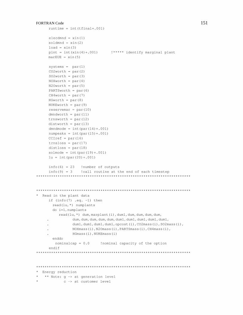
FORTRAN Code 151
runtime = int(tfinal+.001) elecdmnd = xin(1) soldmnd = xin(2) load = xin(3) plnt = int(xin(4)+.001) !***** identify marginal plant marEUE = xin(5) systems = par(1) CO2worth = par(2) SO2worth = par(3) NOXworth = par(4) N2Oworth = par(5) PARTSworth = par(6) CH4worth = par(7) HGworth = par(8) NUKEworth = par(9) reservemar = par(10) dmndworth = par(11) trnsworth = par(12) distworth = par(13) dmndmode = int(par(14)+.001) numpeaks = int(par(15)+.001) CCIref = par(16) trnsloss = par(17) distloss = par(18) solmode = int(par(19)+.001) lu = int(par(20)+.001) info(6) = 23 !number of outputs info(9) = 3 !call routine at the end of each timestep ************************************************************************ ************************************************************************ * Read in the plant data if (info(7) .eq. -1) then read(lu,*) numplants do i=1,numplants read(lu,*) dum,marplant(i),dum1,dum,dum,dum,dum, . dum,dum,dum,dum,dum,dum1,dum1,dum1,dum1,dum1, . dum1,dum1,dum1,dum1,opcost(i),CO2mass(i),SO2mass(i), . NOXmass(i),N2Omass(i),PARTSmass(i),CH4mass(i), . HGmass(i),NUKEmass(i) enddo nominalcap = 0.0 !nominal capacity of the option endif ************************************************************************ ************************************************************************ * Energy reduction * ** Note: g -> at generation level * c -> at customer level

152 FORTRAN Code
TDloss = (1-trnsloss)*(1-distloss) if (solmode .eq. 1) then !*** option reduces electric demand enred_g =(elecdmnd-soldmnd)*systems/TDloss enred_c = (elecdmnd-soldmnd)*systems ensavings = enred_g*opcost(plnt) currentcap = elecdmnd*systems elseif (solmode .eq. 2) then !*** option generates electricity enred_g = soldmnd*systems/TDloss enred_c = soldmnd*systems ensavings = enred_g*opcost(plnt) currentcap = soldmnd*systems else print*, 'ERROR, SOLAR MODE NOT SPECIFIED CORRECTLY' endif if (currentcap .gt. nominalcap) then nominalcap = currentcap endif ************************************************************************ ************************************************************************ * Pollution reduction * Convert pollution savings from kWh to MWh CO2red = enred_g/1000 * CO2mass(plnt) CO2val = CO2red * CO2worth SO2red = enred_g/1000 * SO2mass(plnt) SO2val = SO2red * SO2worth NOXred = enred_g/1000 * NOXmass(plnt) NOXval = NOXred * NOXworth N2Ored = enred_g/1000 * N2Omass(plnt) N2Oval = N2Ored * N2Oworth PARTSred = enred_g/1000 * PARTSmass(plnt) PARTSval = PARTSred * PARTSworth CH4red = enred_g/1000 * CH4mass(plnt) CH4val = CH4red * CH4worth HGred = enred_g/1000 * HGmass(plnt) HGval = HGred * HGworth NUKEred = enred_g/1000 * NUKEmass(plnt) NUKEval = NUKEred * NUKEworth pollsavings = CO2val+SO2val+N2Oval+NOXval+PARTSval+CH4val+HGval . + NUKEval ************************************************************************ ************************************************************************ * Demand/Reliablility calculations: * - Mode 1: Demand based on a given number of peak hours * - Mode 2: System reliability based on the whole year *** Mode 1 - Demand calculations *** if (dmndmode .eq. 1) then if (info(7) .eq. -1) then call intzero(peakhour,numpeaks) call realzero(peakload,numpeaks) call realzero(deldmnd,numpeaks)

FORTRAN Code 153
dmndred = 0.0 trnsred = 0.0 distred = 0.0 dmndsavings = 0.0 CCIoption = 0.0 endif if (load .gt. peakload(numpeaks)) then peakload(numpeaks) = load peakhour(numpeaks) = hrtime deldmnd(numpeaks) = enred_g*(1+reservemar) deltrns(numpeaks) = enred_c/(1-distloss) deldist(numpeaks) = enred_c call sort(peakload,peakhour,deldmnd,deltrns,deldist,numpeaks . ) endif if (hrtime .eq. runtime) then do i=1,numpeaks dmndred = dmndred+deldmnd(i)/numpeaks trnsred = trnsred+deltrns(i)/numpeaks distred = distred+deldist(i)/numpeaks enddo dmndsavings = dmndred*dmndworth + trnsred*trnsworth . + distred*distworth !** average impact at customer level, not really a CCI !** define as energy reduction ratio (CRR) CRR = dmndred*TDloss/(1+reservemar)/nominalcap CCIoption = CRR endif **** end mode1 ****** *** Mode 2 - Reliability calculations elseif (dmndmode .eq. 2) then if (info(7) .eq. -1) then peakload(1) = 0.0 dmndsavings = 0.0 dmndred = 0.0 trnsred = 0.0 distred = 0.0 annwgtdenred = 0.0 !annual weighted energy reduction endif if (load .gt. peakload(1)) then peakload(1) = load peakhour(1) = hrtime deldmnd(1) = enred_g*(1+reservemar) deltrns(1) = enred_c/(1-distloss) deldist(1) = enred_c endif wgtdenred = enred_c*marEUE !hourly weighted energy reduction annwgtdenred = annwgtdenred+wgtdenred if (hrtime .eq. runtime) then CCIoption = annwgtdenred/nominalcap dmndred = CCIoption/CCIref*nominalcap*(1+reservemar) . /TDloss trnsred = CCIoption/CCIref*nominalcap/(1-distloss) distred = CCIoption/CCIref*nominalcap

154 FORTRAN Code
dmndsavings = dmndred*dmndworth + trnsred*trnsworth + . distred*distworth endif **** end mode2 ****** *** Error message if not mode 1 or 2 else print*, 'ERROR, DEMAND MODE NOT SPECIFIED CORRECTLY IN TYPE 71' endif ************************************************************************ ************************************************************************ out(1) = enred_g out(2) = ensavings out(3) = CO2red out(4) = CO2val out(5) = SO2red out(6) = SO2val out(7) = NOXred out(8) = NOXval out(9) = N2Ored out(10) = N2Oval out(11) = PARTSred out(12) = PARTSval out(13) = CH4red out(14) = CH4val out(15) = HGred out(16) = HGval out(17) = NUKEred out(18) = NUKEval out(19) = pollsavings out(20) = dmndred out(21) = dmndsavings out(22) = deldmnd(1) out(23) = CCIoption ************************************************************************ ************************************************************************ return 1 end ************************************************************************ ************************************************************************ subroutine realzero(peak,numpeaks) integer numpeaks,i double precision peak dimension peak(8760) do i = 1,numpeaks peak(i) = 0.0 enddo

FORTRAN Code 155
return end ************************************************************************ ************************************************************************ subroutine intzero(peak,numpeaks) integer numpeaks,peak,i dimension peak(8760) do i = 1,numpeaks peak(i) = 0 enddo return end ************************************************************************ ************************************************************************ subroutine sort(peakload,peakhour,deldmnd,deltrns,deldist,numpeaks . ) integer peakhour,numpeaks,i double precision peakload,deldmnd,deltrns,deldist dimension peakhour(8760),peakload(8760),deldmnd(8760), . deltrns(8760),deldist(8760) do i=1,numpeaks-1 ptr = i first = i+1 do j=first,numpeaks if (peakload(j) .gt. peakload(ptr)) then ptr = j endif enddo call realswap(peakload(i),peakload(ptr)) call intswap(peakhour(i),peakhour(ptr)) call realswap(deldmnd(i),deldmnd(ptr)) call realswap(deltrns(i),deltrns(ptr)) call realswap(deldist(i),deldist(ptr)) enddo return end ************************************************************************ ************************************************************************ subroutine realswap(original,new) double precision original,new,hold hold = original original = new new = hold return

156 FORTRAN Code
end ************************************************************************ ************************************************************************ subroutine intswap(original,new) integer original,new,hold hold = original original = new new = hold return end ************************************************************************

FORTRAN Code 157
TYPE 72: Marginal Plant Predictor subroutine type72 (time,xin,out,t,dtdt,par,info,icntrl,*) implicit none ******************************* ** MARGINAL PLANT PREDICTOR ** ******************************* * Standard TRNSYS declarations double precision xin,out real time,t,dtdt,par integer info,icntrl dimension xin(2),out(5),t(1),dtdt(1),par(1),info(15) * TYPE specific variable declarations integer i,numplants,dmonth1,dday1,umonth1,uday1,dmonth2,dday2, . umonth2,uday2,dwnhrs,outhrs,outtime,simtime,LU,plnt,j, . down1,up1,down2,up2 double precision cap,fullout,partout1,partcap1,partout2,partcap2, . partout3,partcap3,partout4,partcap4,dum,foacap,fsoacap, . foafact,fsoafact,load,totcap,marEUE,marcost,opcost logical plantfind character plant*10 dimension plant(5000),cap(5000),dmonth1(5000),dday1(5000), . umonth1(5000),uday1(5000),dmonth2(5000),dday2(5000), . umonth2(5000),uday2(5000),fullout(5000),partout1(5000), . partcap1(5000),partout2(5000),partcap2(5000),partout3(5000), . partcap3(5000),partout4(5000),partcap4(5000),dwnhrs(5000), . foacap(5000),fsoacap(5000),outhrs(5000),down1(5000), . up1(5000),down2(5000),up2(5000),opcost(5000) ************************************************************************ ************************************************************************ call typeck(1,info,2,1,0) simtime = int(time+.001) load = xin(1) marEUE = xin(2) LU = int(par(1)+.001) info(6) = 3 !number of outputs info(9) = 3 !call routine at end of each timestep ************************************************************************ ************************************************************************ if (info(7) .eq. -1) then read(LU,*) numplants do i = 1,numplants read(LU,*) dum,plant(i),cap(i),dmonth1(i),dday1(i), . umonth1(i),uday1(i),dmonth2(i),dday2(i),umonth2(i),

158 FORTRAN Code
. uday2(i),dwnhrs(i),fullout(i),partout1(i),partcap1(i), . partout2(i),partcap2(i),partout3(i),partcap3(i), . partout4(i),partcap4(i),opcost(i),dum,dum,dum,dum,dum, . dum,dum,dum fullout(i) = fullout(i)/100 partout1(i) = partout1(i)/100 partout2(i) = partout2(i)/100 partout3(i) = partout3(i)/100 partout4(i) = partout4(i)/100 down1(i) = outtime(dmonth1(i),dday1(i)) up1(i) = outtime(umonth1(i),uday1(i)) down2(i) = outtime(dmonth2(i),dday2(i)) up2(i) = outtime(umonth2(i),uday2(i)) dwnhrs(i) = dwnhrs(i)*168 !scheduled outage hours outhrs(i) = up1(i)-down1(i)+up2(i)-down2(i) !est. outage period foafact = (1-fullout(i) - (partcap1(i)*partout1(i)+ . partcap2(i)*partout2(i)+partcap3(i)*partout3(i)+ . partcap4(i)*partout4(i))/cap(i)) foacap(i) = cap(i)*foafact if (dwnhrs(i) .le. outhrs(i)) then if (outhrs(i) .eq. 0) then fsoafact = 1.0 else fsoafact = 1.0 - real(dwnhrs(i))/real(outhrs(i)) endif else fsoafact = 1.0 print*, 'ERROR, ACTUAL OUTAGE PERIOD EXCEEDS SCHEDULED OU .TAGE PERIOD FOR PLANT ',i,', ',plant(i) print* endif fsoacap(i) = fsoafact*foacap(i) enddo endif ************************************************************************ ************************************************************************ plantfind = .false. totcap = 0 do j = 1,numplants if (((simtime.ge.down1(j)).and.(simtime.lt.up1(j))) .or. . ((simtime.ge.down2(j)).and.(simtime.lt.up2(j)))) then totcap = totcap + fsoacap(j) else totcap = totcap + foacap(j) endif if ((totcap .gt. load) .and. (.not. plantfind)) then !find marginal plant plantfind = .true. plnt = j marcost = opcost(j)

FORTRAN Code 159
endif if ((.not.plantfind).and.(j.eq.numplants)) then print*, 'ERROR. MARGINAL PLANT NOT FOUND OR LOAD EXCEEDS TO .TAL CAPACITY AT HOUR ',simtime,'. THE LAST PLANT WILL BE ASSUMED .THE MARGIN.' plnt = j goto 20 endif enddo 20 continue ************************************************************************ ************************************************************************ out(1) = load out(2) = plnt out(3) = marEUE out(4) = marcost out(5) = totcap return 1 end ************************************************************************ ************************************************************************ function outtime(month,day) implicit none integer outtime,month,day if (month .eq. 0) then outtime = 0 elseif (month .eq. 1) then outtime = (day-1)*24 + 1 elseif (month .eq. 2) then outtime = (31+day-1)*24 + 1 elseif (month .eq. 3) then outtime = (59+day-1)*24 + 1 elseif (month .eq. 4) then outtime = (90+day-1)*24 + 1 elseif (month .eq. 5) then outtime = (120+day-1)*24 + 1 elseif (month .eq. 6) then outtime = (151+day-1)*24 + 1 elseif (month .eq. 7) then outtime = (181+day-1)*24 + 1 elseif (month .eq. 8) then outtime = (212+day-1)*24 + 1 elseif (month .eq. 9) then outtime = (243+day-1)*24 + 1 elseif (month .eq. 10) then outtime = (273+day-1)*24 + 1 elseif (month .eq. 11) then

160 FORTRAN Code
outtime = (304+day-1)*24 + 1 elseif (month .eq. 12) then outtime = (334+day-1)*24 + 1 endif end

FORTRAN Code 161
TYPE 88: Quick Econonomic Summary subroutine type88 (time,xin,out,t,dtdt,par,info,icntrl,*) ***************************** ** QUICK ECONOMIC ANALYSIS ** ***************************** implicit none * Standard TRNSYS declarations COMMON /SIM/ TIME0,TFINAL,DELT,IWARN double precision xin,out real time,t,dtdt,par,tfinal,time0,delt,iwarn integer info,icntrl dimension xin(7),out(3),t(1),dtdt(1),par(10),info(15) * Economic variable declarations double precision PresWorth,investment,delay,retention,inf,dis, . energy,demand,pollution,oandm,syscost,PWF,levelcost, . taxbracket,depreciation,maxdif,ror,PW,A,B,C,D,dPW, . dPWF_d,downpay,lease,taxcredit,subsidy,numsys,numyrs, . depyrs integer lc,found,runtime,simtime ************************************************************************ ************************************************************************ call typeck(1,info,7,10,0) simtime = int(time+.001) runtime = int(tfinal+.001) energy = xin(1) demand = xin(2) pollution = xin(3) delay = xin(4) subsidy = xin(5) numsys = xin(6) retention = xin(7) numyrs = par(1) inf = par(2) dis = par(3) syscost = par(4) downpay = par(5) lease = par(6) oandm = par(7) taxbracket = par(8) depyrs = par(9) taxcredit = par(10) info(6) = 3 !number of outputs info(9) = 3 !call routine at the end of each timestep
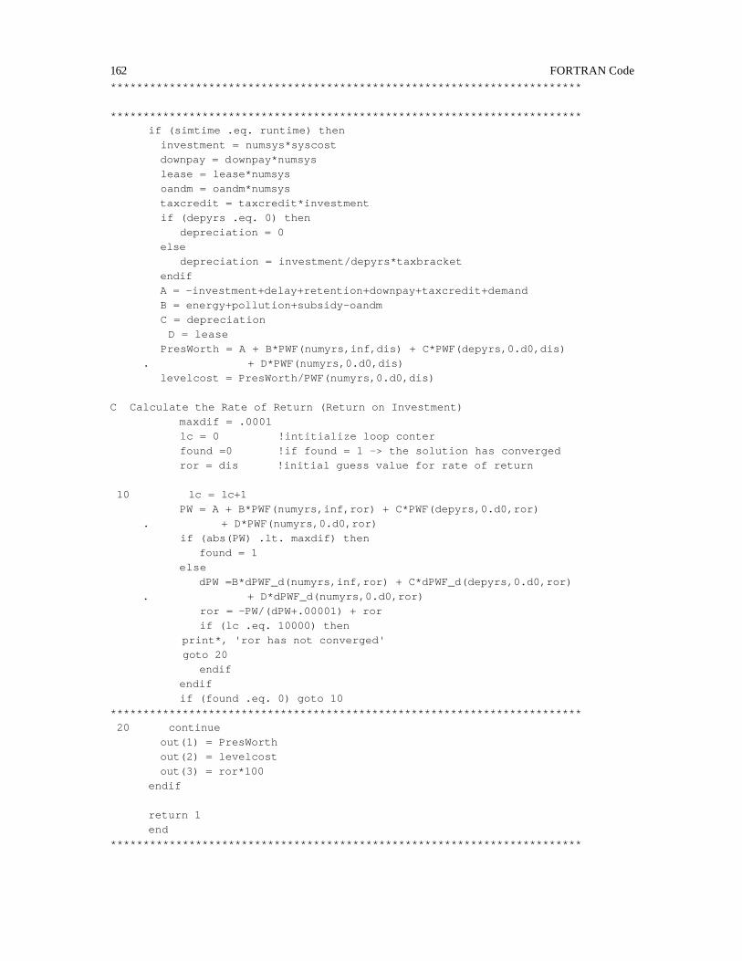
162 FORTRAN Code
************************************************************************ ************************************************************************ if (simtime .eq. runtime) then investment = numsys*syscost downpay = downpay*numsys lease = lease*numsys oandm = oandm*numsys taxcredit = taxcredit*investment if (depyrs .eq. 0) then depreciation = 0 else depreciation = investment/depyrs*taxbracket endif A = -investment+delay+retention+downpay+taxcredit+demand B = energy+pollution+subsidy-oandm C = depreciation D = lease PresWorth = A + B*PWF(numyrs,inf,dis) + C*PWF(depyrs,0.d0,dis) . + D*PWF(numyrs,0.d0,dis) levelcost = PresWorth/PWF(numyrs,0.d0,dis) C Calculate the Rate of Return (Return on Investment) maxdif = .0001 lc = 0 !intitialize loop conter found =0 !if found = 1 -> the solution has converged ror = dis !initial guess value for rate of return 10 lc = lc+1 PW = A + B*PWF(numyrs,inf,ror) + C*PWF(depyrs,0.d0,ror) . + D*PWF(numyrs,0.d0,ror) if (abs(PW) .lt. maxdif) then found = 1 else dPW =B*dPWF_d(numyrs,inf,ror) + C*dPWF_d(depyrs,0.d0,ror) . + D*dPWF_d(numyrs,0.d0,ror) ror = -PW/(dPW+.00001) + ror if (lc .eq. 10000) then print*, 'ror has not converged' goto 20 endif endif if (found .eq. 0) goto 10 ************************************************************************ 20 continue out(1) = PresWorth out(2) = levelcost out(3) = ror*100 endif return 1 end ************************************************************************

FORTRAN Code 163
TYPE 89: Economic Summary
subroutine type89 (time,xin,out,t,dtdt,par,info,icntrl,*) *********************** ** ECONOMIC ANALYSIS ** *********************** implicit none * Standard TRNSYS declarations COMMON /SIM/ TIME0,TFINAL,DELT,IWARN double precision xin,out real time,t,dtdt,par,tfinal,time0,delt,iwarn integer info,icntrl dimension xin(4),out(16),t(1),dtdt(1),par(13),info(15) * Economic variable declarations double precision PresWorth,investment,delay,retention,inf,dis, . energy,demand,pollution,oandm,syscost,PWF,levelcost, . taxbracket,depreciation,maxdif,ror,PW,A,B,C,D,dPW, . dPWF_d,downpay,lease,taxcredit,subsidy,DmndWorth,numsys, . numyrs,depyrs,energyPW,pollutionPW,oandmPW,leasePW, . subsidyPW,depreciationPW integer lc,found,runtime,simtime ************************************************************************ ************************************************************************ call typeck(1,info,5,12,0) simtime = int(time+.001) runtime = int(tfinal+.001) energy = xin(1) demand = xin(2) pollution = xin(3) delay = xin(4) subsidy = xin(5) numyrs = par(1) inf = par(2) dis = par(3) numsys = par(4) syscost = par(5) downpay = par(6) lease = par(7) oandm = par(8) retention = par(9) taxbracket = par(10) depyrs = par(11) taxcredit = par(12) info(6) = 3 !number of outputs

164 FORTRAN Code
info(9) = 3 !call routine at the end of each timestep ************************************************************************ ************************************************************************ if (simtime .eq. runtime) then investment = numsys*syscost downpay = downpay*numsys lease = lease*numsys oandm = oandm*numsys taxcredit = taxcredit*investment if (depyrs .eq. 0) then depreciation = 0 else depreciation = investment/depyrs*taxbracket endif A = -investment+delay+retention+downpay+taxcredit+demand B = energy+pollution+subsidy-oandm energyPW = energy*PWF(numyrs,inf,dis) pollutionPW = pollution*PWF(numyrs,inf,dis) subsidyPW = subsidy*PWF(numyrs,inf,dis) oandmPW = oandm*PWF(numyrs,inf,dis) C = depreciation depreciationPW = C*PWF(depyrs,0.d0,dis) D = lease leasePW = D*PWF(numyrs,0.d0,dis) PresWorth = A + B*PWF(numyrs,inf,dis) + C*PWF(depyrs,0.d0,dis) . + D*PWF(numyrs,0.d0,dis) levelcost = PresWorth/PWF(numyrs,0.d0,dis) DmndWorth = demand/PWF(numyrs,inf,dis) C Calculate the Rate of Return (Return on Investment) maxdif = .0001 lc = 0 !intitialize loop conter found = 0 !if found = 1 -> the solution has converged ror = dis !initial guess value for rate of return 10 lc = lc+1 PW = A + B*PWF(numyrs,inf,ror) + C*PWF(depyrs,0.d0,ror) . + D*PWF(numyrs,0.d0,ror) if (abs(PW) .lt. maxdif) then found = 1 else dPW = B*dPWF_d(numyrs,inf,ror) + C*dPWF_d(depyrs,0.d0,ror) . + D*dPWF_d(numyrs,0.d0,ror) ror = -PW/dPW + ror if (lc .eq. 10000) then print*, 'ror has not converged' goto 20 endif endif if (found .eq. 0) goto 10 ************************************************************************ 20 continue

FORTRAN Code 165
out(1) = PresWorth out(2) = levelcost out(3) = ror*100 out(4) = DmndWorth out(5) = investment out(6) = delay out(7) = retention out(8) = downpay out(9) = taxcredit out(10) = demand out(11) = energyPW out(12) = pollutionPw out(13) = subsidyPW out(14) = oandmPW out(15) = depreciationPW out(16) = leasePW endif return 1 end ************************************************************************ ************************************************************************ function PWF(N,i,d) double precision i,d,N,PWF if (i.eq.d) then PWF = N/(1+i) else PWF = (1-((1+i)/(1+d))**N)/(d-i) endif return end ************************************************************************ ************************************************************************ function dPWF_d(N,i,d) double precision i,d,N,dPWF_d,PWF if (i.eq.d) then dPWF_d = -N/(d+1)**2 else dPWF_d = (N/(1+d)*((1+i)/(1+d))**N-PWF(N,i,d))/(d-i) endif return end ************************************************************************
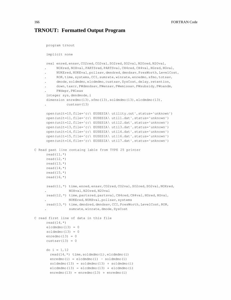
166 FORTRAN Code
TRNOUT: Formatted Output Program
program trnout implicit none real enred,ensav,CO2red,CO2val,SO2red,SO2val,N2Ored,N2Oval, . NOXred,NOXval,PARTSred,PARTSval,CH4red,CH4val,HGred,HGval, . NUKEred,NUKEval,pollsav,dmndred,dmndsav,PresWorth,LevelCost, . ROR,time,systems,CCI,sumrate,winrate,enredmo,sfmo,totsav, . dmode,soldmdmo,elcdmdmo,custsav,SysCost,delay,retention, . down,taxcr,PWdmndsav,PWensav,PWemissav,PWsubsidy,PWoandm, . PWdepr,PWleas integer sys,dmndmode,i dimension enredmo(13),sfmo(13),soldmdmo(13),elcdmdmo(13), . custsav(13) open(unit=10,file='c:\ EUSESIA\ utility.out',status='unknown') open(unit=11,file='c:\ EUSESIA\ util1.dat',status='unknown') open(unit=12,file='c:\ EUSESIA\ util2.dat',status='unknown') open(unit=13,file='c:\ EUSESIA\ util3.dat',status='unknown') open(unit=14,file='c:\ EUSESIA\ util4.dat',status='unknown') open(unit=15,file='c:\ EUSESIA\ util6.dat',status='unknown') open(unit=16,file='c:\ EUSESIA\ util7.dat',status='unknown') C Read past line containg lable from TYPE 25 printer read(11,*) read(12,*) read(13,*) read(14,*) read(15,*) read(16,*) read(11,*) time,enred,ensav,CO2red,CO2val,SO2red,SO2val,NOXred, . NOXval,N2Ored,N2Oval read(12,*) time,partsred,partsval,CH4red,CH4val,HGred,HGval, . NUKEred,NUKEval,pollsav,systems read(13,*) time,dmndred,dmndsav,CCI,PresWorth,LevelCost,ROR, . sumrate,winrate,dmode,SysCost C read first line of data in this file read(14,*) elcdmdmo(13) = 0 soldmdmo(13) = 0 enredmo(13) = 0 custsav(13) = 0 do i = 1,12 read(14,*) time,soldmdmo(i),elcdmdmo(i) enredmo(i) = elcdmdmo(i) - soldmdmo(i) soldmdmo(13) = soldmdmo(13) + soldmdmo(i) elcdmdmo(13) = elcdmdmo(13) + elcdmdmo(i) enredmo(13) = enredmo(13) + enredmo(i)

FORTRAN Code 167
enddo read(15,*) time,delay,retention,down,taxcr,PWdmndsav,PWensav, . PWemissav,PWsubsidy,PWoandm,PWdepr read(16,*) time,PWleas if (elcdmdmo(13) .ne. 0) then do i=1,5 custsav(i) = enredmo(i)*winrate enddo do i=6,9 custsav(i) = enredmo(i)*sumrate enddo do i=10,12 custsav(i) = enredmo(i)*winrate enddo do i=1,13 sfmo(i) = enredmo(i)/elcdmdmo(i) enddo do i=1,12 custsav(13) = custsav(13) + custsav(i) enddo else do i=1,5 custsav(i) = soldmdmo(i)*winrate enddo do i=6,9 custsav(i) = soldmdmo(i)*sumrate enddo do i=10,12 custsav(i) = soldmdmo(i)*winrate enddo do i=1,12 custsav(13) = custsav(13) + custsav(i) enddo endif totsav = ensav+pollsav+dmndsav sys = int(systems+.001) dmndmode = int(dmode+.001) SysCost = SysCost*real(sys) write(10,*) write(10,*) ' Electric Utility Solar Energy System Im .pact Analysis:' write(10,*) write(10,*) ' Impact of a Large Scale Implemention of a S .olar Energy System' write(10,*) ' on an Electric Utility' write(10,*) write(10,*) '****** Energy and Environmental Impact Summary for t .he First Year ******' write(10,200) sys

168 FORTRAN Code
write(10,*) write(10,*) ' Energy Reduction (kWh) Energy Savings . ($)' write(10,100) enred,ensav write(10,*) write(10,*) ' Emission Reduction (lbm) Emission Savin .gs ($) ' write(10,101) CO2red,CO2val write(10,102) SO2red,SO2val write(10,103) NOXred,NOXval write(10,104) N2Ored,N2Oval write(10,105) partsred,partsval write(10,106) CH4red,CH4val write(10,107) HGred,HGval write(10,108) NUKEred,NUKEval write(10,109) pollsav write(10,*) write(10,*) ' Demand Reduction (kW) Demand Savings . ($) ' write(10,110) dmndred,dmndsav write(10,*) write(10,*) ' Total Savings .($) ' write(10,111) totsav write(10,*) write(10,*) '****** Economic Analysis Summary ****************** .***********************' write(10,*) write(10,300) SysCost write(10,301) PWoandm write(10,302) PWensav write(10,303) PWemissav write(10,304) PWdmndsav write(10,305) PWdepr write(10,306) down write(10,307) PWleas write(10,308) taxcr write(10,309) PWsubsidy write(10,310) retention write(10,311) delay write(10,*) write(10,312) PresWorth write(10,313) LevelCost write(10,314) ROR write(10,*) write(10,*) '****** System Performance Summary and Customer Savin .gs *******************' write(10,*) ' Results based on average system performance' write(10,*) IF (INT(elcdmdmo(13)-.001) .ne. 0) THEN write(10,*) ' Elc (kWh) Sol (kWh) Del (kWh) SF . Savings ($) ' write(10,401) elcdmdmo(1),soldmdmo(1),enredmo(1),sfmo(1), . custsav(1)

FORTRAN Code 169
write(10,402) elcdmdmo(2),soldmdmo(2),enredmo(2),sfmo(2), . custsav(2) write(10,403) elcdmdmo(3),soldmdmo(3),enredmo(3),sfmo(3), . custsav(3) write(10,404) elcdmdmo(4),soldmdmo(4),enredmo(4),sfmo(4), . custsav(4) write(10,405) elcdmdmo(5),soldmdmo(5),enredmo(5),sfmo(5), . custsav(5) write(10,406) elcdmdmo(6),soldmdmo(6),enredmo(6),sfmo(6), . custsav(6) write(10,407) elcdmdmo(7),soldmdmo(7),enredmo(7),sfmo(7), . custsav(7) write(10,408) elcdmdmo(8),soldmdmo(8),enredmo(8),sfmo(8), . custsav(8) write(10,409) elcdmdmo(9),soldmdmo(9),enredmo(9),sfmo(9), . custsav(9) write(10,410) elcdmdmo(10),soldmdmo(10),enredmo(10),sfmo(10), . custsav(10) write(10,411) elcdmdmo(11),soldmdmo(11),enredmo(11),sfmo(11), . custsav(11) write(10,412) elcdmdmo(12),soldmdmo(12),enredmo(12),sfmo(12), . custsav(12) write(10,*) write(10,413) elcdmdmo(13),soldmdmo(13),enredmo(13),sfmo(13), . custsav(13) write(10,*) ELSE write(10,*) ' ElcGen (kWh) Savings ($) ' write(10,501) soldmdmo(1),custsav(1) write(10,502) soldmdmo(2),custsav(2) write(10,503) soldmdmo(3),custsav(3) write(10,504) soldmdmo(4),custsav(4) write(10,505) soldmdmo(4),custsav(5) write(10,506) soldmdmo(6),custsav(6) write(10,507) soldmdmo(7),custsav(7) write(10,508) soldmdmo(8),custsav(8) write(10,509) soldmdmo(9),custsav(9) write(10,510) soldmdmo(10),custsav(10) write(10,511) soldmdmo(11),custsav(11) write(10,512) soldmdmo(12),custsav(12) write(10,*) write(10,513) soldmdmo(13),custsav(13) ENDIF write(10,*) IF (dmndmode .eq. 1) THEN write(10,*) ' Option Capacity Reduction Ratio' write(10,112) CCI ELSE write(10,*) ' Option Capacity Contribution Index ' write(10,112) CCI ENDIF

170 FORTRAN Code
100 FORMAT(' ',F12.0,' ',F12.0,' .') 101 FORMAT(' CO2 ',F12.0,' ',F12.0,' .') 102 FORMAT(' SO2 ',F12.0,' ',F12.0,' .') 103 FORMAT(' NOX ',F12.0,' ',F12.0,' .') 104 FORMAT(' N2O ',F12.0,' ',F12.0,' .') 105 FORMAT(' Parts ',F12.0,' ',F12.0,' .') 106 FORMAT(' CH4 ',F12.0,' ',F12.0,' .') 107 FORMAT(' HG ',F12.0,' ',F12.0,' .') 108 FORMAT(' NUKES ',F12.0,' ',F12.0,' .') 109 FORMAT(' ',F12.0,' . ') 110 FORMAT(' ',F12.0,' ',F12.0,' . ') 111 FORMAT(' ',F12.0,' . ') 112 FORMAT(' ',F12.3) 200 FORMAT(' Results based on:',I5,' solar systems') 300 FORMAT(' Present Worth of Investment - $',F14.0,' ') 301 FORMAT(' Present Worth of O&M - $',F14.0,' ') 302 FORMAT(' Present Worth of Energy Savings $',F14.0,' ') 303 FORMAT(' Present Worth of Emission Savings $',F14.0,' ') 304 FORMAT(' Present Worth of Demand Savings $',F14.0,' ') 305 FORMAT(' Present Worth of Depreciation $',F14.0,' ') 306 FORMAT(' Present Worth of Downpayments $',F14.0,' ') 307 FORMAT(' Present Worth of Lease Payments $',F14.0,' ') 308 FORMAT(' Present Worth of Tax Credit $',F14.0,' ') 309 FORMAT(' Present Worth of Energy Subsidy $',F14.0,' ') 310 FORMAT(' Present Worth of Customer Retention $',F14.0,' ') 311 FORMAT(' Present Worth of Delay Value $',F14.0,' ') 312 FORMAT(' Present Worth of Life Cycle Savings $',F14.0,' ') 313 FORMAT(' Levelized Savings of Option $',F14.0,' ') 314 FORMAT(' Rate of Invstment of Option ',F6.1,' % . ') 401 FORMAT(' JAN ',F6.0,' ',F6.0,' ',F6.0,' ',F4. .3,' ',F6.2,' ') 402 FORMAT(' FEB ',F6.0,' ',F6.0,' ',F6.0,' ',F4. .3,' ',F6.2,' ') 403 FORMAT(' MAR ',F6.0,' ',F6.0,' ',F6.0,' ',F4. .3,' ',F6.2,' ')

FORTRAN Code 171
404 FORMAT(' APR ',F6.0,' ',F6.0,' ',F6.0,' ',F4. .3,' ',F6.2,' ') 405 FORMAT(' MAY ',F6.0,' ',F6.0,' ',F6.0,' ',F4. .3,' ',F6.2,' ') 406 FORMAT(' JUN ',F6.0,' ',F6.0,' ',F6.0,' ',F4. .3,' ',F6.2,' ') 407 FORMAT(' JUL ',F6.0,' ',F6.0,' ',F6.0,' ',F4. .3,' ',F6.2,' ') 408 FORMAT(' AUG ',F6.0,' ',F6.0,' ',F6.0,' ',F4. .3,' ',F6.2,' ') 409 FORMAT(' SEP ',F6.0,' ',F6.0,' ',F6.0,' ',F4. .3,' ',F6.2,' ') 410 FORMAT(' OCT ',F6.0,' ',F6.0,' ',F6.0,' ',F4. .3,' ',F6.2,' ') 411 FORMAT(' NOV ',F6.0,' ',F6.0,' ',F6.0,' ',F4. .3,' ',F6.2,' ') 412 FORMAT(' DEC ',F6.0,' ',F6.0,' ',F6.0,' ',F4. .3,' ',F6.2,' ') 413 FORMAT(' YEAR ',F6.0,' ',F6.0,' ',F6.0,' ',F4. .3,' ',F6.2,' ') 501 FORMAT(' JAN ',F6.0,' ',F6.2,' ') 502 FORMAT(' FEB ',F6.0,' ',F6.2,' ') 503 FORMAT(' MAR ',F6.0,' ',F6.2,' ') 504 FORMAT(' APR ',F6.0,' ',F6.2,' ') 505 FORMAT(' MAY ',F6.0,' ',F6.2,' ') 506 FORMAT(' JUN ',F6.0,' ',F6.2,' ') 507 FORMAT(' JUL ',F6.0,' ',F6.2,' ') 508 FORMAT(' AUG ',F6.0,' ',F6.2,' ') 509 FORMAT(' SEP ',F6.0,' ',F6.2,' ') 510 FORMAT(' OCT ',F6.0,' ',F6.2,' ') 511 FORMAT(' NOV ',F6.0,' ',F6.2,' ') 512 FORMAT(' DEC ',F6.0,' ',F6.2,' ') 513 FORMAT(' YEAR ',F6.0,' ',F6.2,' ') close(10) close(11) close(12) close(13) close(14) close(15) close(16) return end