Virginia Commonwealth University Virginia Commonwealth University

VCU Scholars Compass VCU Scholars Compass

Theses and Dissertations Graduate School

2019

Electric Load Forecasting Using Long Short-term Memory Electric Load Forecasting Using Long Short-term Memory

Algorithm Algorithm

Tianshu Yang

Follow this and additional works at: https://scholarscompass.vcu.edu/etd

Part of the Electrical and Electronics Commons, and the Power and Energy Commons

© The Author

Downloaded from Downloaded from https://scholarscompass.vcu.edu/etd/6027

This Thesis is brought to you for free and open access by the Graduate School at VCU Scholars Compass. It has been accepted for inclusion in Theses and Dissertations by an authorized administrator of VCU Scholars Compass. For more information, please contact libcompass@vcu.edu.

Copyright © 2019 Tianshu Yang. All rights reserved.

2

3

Electric Load Forecasting Using Long Short-

term Memory Algorithm

A dissertation submitted in partial fulfillment of the requirements for the degree of

Master of Philosophy at Virginia Commonwealth University

By

Tianshu Yang

M.S in Electrical Engineering

Advisor: Zhifang Wang, Ph.D.

Associate Professor, Department of Electrical and Computer Engineering

Virginia Commonwealth University

Richmond, Virginia

July 2019

4

Acknowledgment I want to recognize Professor Zhifang Wang for her support and help throughout the study,

which enabled me to understand the principles and operations of the entire model more

thoroughly and to implement this project. Her support and help are that I better use software

to model and optimize theoretical principles to improve and achieve satisfactory results

and data.

I would also like to thank Dr. Motai and Dr. Thang Dinh, who agreed to be a member of

this committee.

5

Table of Contents

ACKNOWLEDGMENT ..................................................................................................... 4

ABSTRACT ......................................................................................................................... 9

1.1 APPLICATION OF LOAD FORECASTING .................................................................... 10

1.2 BASIC METHOD OF LOAD FORECASTING ................................................................. 11

1.2.1 Neural network method ............................................................................................................... 11

1.2.2 Time series method ...................................................................................................................... 11

1.2.3 Regression analysis ..................................................................................................................... 12

1.3 MOTIVATION OF THE LSTM ................................................................................... 12

1.4 CHALLENGES OF THE LSTM ................................................................................... 13

A. hardware acceleration ...................................................................................................................... 13

B. Vanishing gradients ......................................................................................................................... 13

1.5 CONTRIBUTIONS ...................................................................................................... 13

2 DEEP LEARNING ........................................................................................................ 15

2.1 PERCEPTRON ........................................................................................................... 16

2.2 LINEAR UNIT ............................................................................................................ 16

2.3 SUPERVISED LEARNING AND UNSUPERVISED LEARNING ........................................ 17

2.4 THE OBJECTIVE FUNCTION OF A LINEAR UNIT ....................................................... 17

2.5 GRADIENT DESCENT OPTIMIZATION ALGORITHM ................................................. 19

2.5.1 Derivation of ∇E(w) .................................................................................................................... 20

2.6 STOCHASTIC GRADIENT DESCENT, SGD ............................................................... 21

3 ARTIFICIAL NEURAL NETWORK ........................................................................... 23

3.1 NEURONS ................................................................................................................. 25

3.2 CALCULATE THE OUTPUT OF THE NEURAL NETWORK ........................................... 26

3.3 BACK PROPAGATION ............................................................................................... 28

3.4 DERIVATION OF THE BACKPROPAGATION ALGORITHM ......................................... 30

3.4.1 Output layer weight training ........................................................................................................ 32

3.4.2 Hidden layer weight training ....................................................................................................... 33

6

4 RECURRENT NEURAL NETWORK .......................................................................... 35

4.1 BASIC RECURRENT NEURAL NETWORK ................................................................. 35

4.2 TRAINING ALGORITHM FOR RECURRENT NEURAL NETWORKS: BPTT .............. 36

5 LONG SHORT-TERM MEMORY NETWORK .......................................................... 43

5.1 FORWARD CALCULATION OF LSTM ...................................................................... 44

5.1.1 Forgotten gate .............................................................................................................................. 45

5.1.2 Input gate ..................................................................................................................................... 46

5.1.3 Output gate .................................................................................................................................. 48

5.1.4 Final output .................................................................................................................................. 49

6 TRAINING OF THE LSTM ......................................................................................... 50

6.1 TRAINING PROCESS OF LSTM IN MATLAB ............................................................ 50

6.1.1 Initial Weights and Biases ........................................................................................................... 51

6.1.2 Initial learning rate ...................................................................................................................... 51

6.2 TRAINING PROCESS RESULTS .................................................................................. 51

7 PREDICT RESULTS .................................................................................................... 56

7.1 PREDICT AND UPDATE STATE ................................................................................. 56

7.1.1 PREDICT BY THE TRAINING MODEL ...................................................................... 56

7.2 CONCLUSION OF THE PREDICT RESULT .................................................................. 62

8 CONCLUSION AND FUTURE WORK ....................................................................... 63

REFERENCES ................................................................................................................. 64

7

List of Figures FIGURE1. STRUCTURE OF THE NEURAL NETWORK .......................................... 15

FIGURE 2. STRUCTURE OF PERCEPTRON ............................................................. 16

FIGURE 3. STRUCTURE OF THE LINEAR UNIT ..................................................... 16

FIGURE 4. OPTIMIZATION OF GRADIENT DESCENT .......................................... 19

FIGURE 5. DIFFERENCE BETWEEN SGD AND BGD. ........................................... 22

FIGURE 6. FULL CONNECTED NEURAL NETWORKS .......................................... 24

FIGURE 7. STRUCTURE OF A NEURON ................................................................... 25

FIGURE 8. SIGMOID FUNCTION ............................................................................... 26

FIGURE 9 NEURAL NETWORK ................................................................................... 27

FIGURE 10. NEURAL NETWORK ................................................................................ 29

FIGURE 11. NEURAL NETWORK ................................................................................ 31

FIGURE 12. RECURRENT NEURAL NETWORK ....................................................... 35

FIGURE 13. RECURRENT LAYER ............................................................................... 36

FIGURE 14 RECURRENT LAYER ................................................................................ 40

FIGURE 15. TRANSMISSION IN LSTM ..................................................................... 44

FIGURE 16. CALCULATION OF THE FORGOTTEN GATE .................................... 46

FIGURE 17. CALCULATION OF 𝒊𝒕 IN THE INPUT GATE .................................... 46

FIGURE 18. CALCULATION OF 𝒄𝒕 IN THE INPUT GATE .................................... 47

FIGURE 19. CALCULATION OF 𝒄𝒕 IN THE INPUT GATE .................................... 48

FIGURE 20. CALCULATION OF THE OUTPUT GATE ............................................ 49

FIGURE 21. CALCULATION OF THE FINAL OUTPUT ........................................... 49

FIGURE 22. TRAINING PROCESS WITH LEARNING RATE 0.001 ........................ 52

FIGURE 23. TRAINING PROCESS WITH LEARNING RATE 0.01 .......................... 52

8

FIGURE 24. TRAINING PROCESS WITH LEARNING RATE 0.1 ............................ 53

FIGURE 25. TRAINING PROCESS WITH TIME STEPS SIZE IS 50 ....................... 54

FIGURE 26. TRAINING PROCESS WITH TIME STEPS SIZE IS 300 ..................... 55

FIGURE 27. TRAINING PROCESS WITH TIME STEPS SIZE IS 600 ..................... 55

FIGURE 28. PREDICT RESULT WHICH UPDATE STATE WITH PREDICT DATA

........................................................................................................................................... 57

FIGURE 29. PREDICT RESULT WITH LEARNING RATE 0.001 ............................ 58

FIGURE 30. PREDICT RESULT WITH LEARNING RATE 0.01 .............................. 58

FIGURE 31. PREDICT RESULT WITH LEARNING RATE 0.1 ................................ 59

FIGURE 32. PREDICT RESULT WITH TIME STEPS SIZE IS 50 ............................ 60

FIGURE 33. PREDICT RESULT WITH TIME STEPS SIZE IS 150 .......................... 60

FIGURE 34. PREDICT RESULT WITH TIME STEPS SIZE IS 300 .......................... 61

FIGURE 35 PREDICT RESULT WITH TIME STEPS SIZE IS 600 ........................... 61

FIGURE 36 SUMMARY OF PREDICT RESULT WITH TIME STEPS SIZE ........... 62

FIGURE 37 SUMMARY OF PREDICT RESULT WITH INITIAL LEARNING RATE

........................................................................................................................................... 62

List of Tables TABLE 1 SUMMARY OF PREDICT RESULT WITH INITIAL LEARNING RATE 62

TABLE 2 SUMMARY OF PREDICT RESULT WITH TIME STEPS SIZE ............... 62

9

Abstract Power system load forecasting refers to the study or uses a mathematical method to process

past and future loads systematically, taking into account important system operating

characteristics, capacity expansion decisions, natural conditions, and social impacts, to

meet specific accuracy requirements. Dependence of this, determine the load value at a

specific moment in the future. Improving the level of load forecasting technology is

conducive to the planned power management, which is conducive to rationally arranging

the grid operation mode and unit maintenance plan, and is conducive to formulating

reasonable power supply construction plans and facilitating power improvement, and

improve the economic and social benefits of the system.

At present, there are many methods for load forecasting. The newer algorithms mainly

include the neural network method, time series method, regression analysis method,

support vector machine method, and fuzzy prediction method. However, most of them do

not apply to long-term time-series predictions, and as a result, the prediction accuracy for

long-term power grids does not perform well.

This thesis describes the design of an algorithm that is used to predict the load in a long

time-series. Predict the load is significant and necessary for a dynamic electrical network.

Improved the forecasting algorithm can save a ton of the cost of the load. In this paper, we

propose a load forecasting model using long short-term memory(LSTM). The proposed

implementation of LSTM match with the time-series dataset very well, which can improve

the accuracy of convergence of the training process. We experiment with the difference

time-step to expedites the convergence of the training process. It is found that all cases

achieve significant different forecasting accuracy while forecasting the difference time-

steps.

Keywords—Load forecasting, long short-term memory, micro-grid

10

1 Introduction Electric load forecasting has become one of the required fields in power engineering. The

desirable forecast method can achieve satisfactory forecasting accuracy without high

computation cost. Load forecasting can maintain the safety and stability of the grid

operation, reduce the unnecessary rotating reserve capacity, and rationally arrange the unit

maintenance plan. To ensure the average production and life of the society, effectively

reduce the cost of power generation, and improve economic and social benefits

The results of load forecasting can also help determine the installation of new generator

sets in the future, determine the size, location and time of installed capacity, determine the

capacity expansion and reconstruction of the power grid, and determine the construction

and development of the power grid.

Therefore, the level of power load forecasting work has become one of the significant

indicators to measure whether an electrical network system management is modernizing.

Power load forecasting has become an important and arduous task to solve the problem of

electricity management.

In this paper, we pay attention to solving the problem to deal with the long-time data

forecasting in the electrical network. We try to find a new Neural network algorithm that

can give a higher forecasting accuracy in a long time sequence.

1.1 application of load forecasting Load forecasting (electric load forecasting, power demand forecasting). Although "load"

is a vague term, in load forecasting, "load" usually means demand (in kW) or energy (in

kWh), and because the power and energy of the hourly data are the same, Therefore, it is

usually not necessary to distinguish between demand and energy. Load forecasting

involves accurate prediction of size and geographic location at different times during the

planning period. The necessary amount of interest is usually the total system (or area) load

per hour. However, load forecasting also involves hourly, daily, weekly, and monthly load

and peak load forecasts.

Load forecasting is a technique used by electricity or energy supply companies to predict

the power/energy needed to satisfy demand and supply equilibrium. The accuracy of the

11

forecast is essential to the operational and management of the load in a utility electrical

network.

Load forecasting has long been considered the initial building block for all utility planning

efforts, and it will decide the expected future energy sales and peak demand. The benefits

of reasonable and accurate load forecasts are not only manifested in the economic field but

also bring positive benefits to the development of the whole society. Therefore, the method

of load forecasting is becoming more and more popular, and new methods are continually

being put into use and continuously be improved.

1.2 Basic method of load forecasting Due to various factors such as weather changes, social activities and festival types, the load

appears as a non-stationary random process in time series, but most of the factors affecting

system load have regularity, to achieve effective prediction. Foundation. In order to predict

the load better, people use many methods to increase the accuracy of the short-term load.

The newer algorithms mainly include the neural network method, time series method,

regression analysis method, support vector machine method, and fuzzy prediction

method[2]. The core problem of power load forecasting research is how to use existing

historical data to establish a predictive model to predict the load value in future time or

period. Therefore, the reliability of historical data information and prediction model are the

central factors that affect load forecasting accuracy.

1.2.1 Neural network method

The neural network method is currently the most advanced load forecasting method. The

application of neural network method in load forecasting is mainly divided into an artificial

neural network (ANN) and recurrent neural network (also known as a recurrent neural

network, referred to as RNN). Among them, RNN is an algorithm that works better than

ANN. LSTM is an advanced neural network algorithm, and we will discuss its technical

details in the following sections.[2]

1.2.2 Time series method

The historical data of the power load is an ordered set of samples and records at regular

intervals is a time series. The time series method is based on historical data of load by using

12

a mathematical model describing the change of electrical load. Based on the model,

establish the expression of the load forecast, and predict the future load.

The model has high requirements for the stationarity of the original time series, and is only

suitable for short-term predictions with uniform load changes; If this model meets

instability factors such as weather, holidays, the predicted result will have a huge error.

1.2.3 Regression analysis

The regression analysis prediction method is based on the change rule of historical data

and the factors affecting the load change, find the correlation between the independent

variable and the dependent variable; get its regression equation, determine the model

parameters; and predict the load value at the later time.

The shortcomings are that the historical data is relatively high, and the linear method is

used to describe the complicated problems. The structural form is too pure, and the

precision is not excellent. The model cannot describe various factors affecting the load in

detail. The model's initialization is complicated and needs abundant Experience and skills.

1.3 motivation of the LSTM The emergence of RNNs is mainly because they can link the previous information to the

present and solve the current problems. For example, using the previous screen can help us

understand the content of the current screen. If RNNs can do this, then it is helpful for our

mission.

Sometimes, when we are dealing with the current task, we only need to look at some of the

more recent information. When need to predict a sentence word while it only has tens of

letter, the RNN will be okay. However, while the number of the letter increasing to

hundreds or thousands, the predicted error will increase fast. As the interval between

prediction information and related information increases, it is difficult for RNNs to

associate them.

In theory, RNNs can link such long-term dependencies ("long-term dependencies") and

solve such problems by choosing the right parameters. However, unfortunately, in practice,

RNNs can't solve this problem.

However, fortunately, LSTMs can help us solve this problem. The LSTM algorithm is a

neural network algorithm used to predict long-term time series. It can significantly improve

13

the gradient explosion and gradient disappearance of neural network algorithms in the face

of long time series data.[1]

1.4 challenges of the LSTM A. hardware acceleration

A big problem with LSTM is that training them requires very high hardware. Also, it still

requires many resources when we do not need to train these networks quickly. Running

these models in the same cloud also requires a lot of resources. Training the nightmare of

LSTM, LSTM training is difficult because they require storage bandwidth binding

calculations, which is the worst nightmare for hardware designers and ultimately limits the

applicability of neural network solutions. In short, LSTM requires four linear layers per

unit to run in each sequence time step. Linear layers require a large amount of storage

bandwidth to calculate. They cannot use many computing units, usually because the system

does not have enough storage bandwidth to satisfy the computing unit. Moreover, it is easy

to add more compute units, but it is hard to add more storage bandwidth (note that there

are enough wires on the chip, from the processor to the long wires stored). Therefore,

LSTM and its variants are not a good match for hardware acceleration.

B. Vanishing gradients

LSTM can reduce the problem of gradient disappearance (explosion) to a certain extent,

but in essence, it's training still follows a sequential path from the past unit to the current

unit. Moreover, this path is now more complicated, adding a lot of additional components.

This path can now remember historical information for an extended time-series, but it is

not infinite. As the number of time series increases, the degree of retention of historical

information will decrease. Therefore LSTM is generally applied to sequences of 100 orders

of magnitude instead of 1000 orders of magnitude, or longer sequences.

1.5 contributions With the develop research of the LSTM algorithm, the application of LSTM has been

continuously promoted, but the implementation of LSTM in long-term prediction of the

power grid is rare. People still prefer to use the traditional RNN algorithm for prediction.

Therefore, this paper focuses on the application of LSTM in the field of load forecasting

14

and compares the prediction efficiency and accuracy of the algorithm under different time

series. In this process, we can find a more optimal prediction model.

This thesis describes the design of an algorithm that is used to predict the load in a long

time-series. Predict the load is significant and necessary for a dynamic electrical network.

Improved the forecasting algorithm can save a ton of the cost of the load. In this paper, we

propose a load forecasting model using long short-term memory(LSTM). The proposed

implementation of LSTM match with the time-series dataset very well, which can improve

the accuracy of convergence of the training process. We experiment with the difference

time-step to expedites the convergence of the training process. It is found that all cases

achieve significant different forecasting accuracy while forecasting the difference time-

steps.

15

2 Deep learning There is a method called machine learning in the field of artificial intelligence. In the

machine learning method, there is a class of algorithms called neural networks. The neural

network is shown below[14]:

Figure1. structure of the neural network

Each circle in the above picture is a neuron, and each line represents the connection

between neurons. We can see that the above neurons are divided into multiple layers, the

neurons between the layers are connected, and the neurons in the layers are not connected.

The leftmost layer is called the input layer. This layer is responsible for receiving input

data. The rightmost layer is called the output layer. We can get the neural network output

data from this layer. The layer between the input layer and the output layer is called a

hidden layer.

A neural network with more hidden layers (greater than 2) is called a deep neural network.

deep learning is one of the branch which use machine learning method in deep

architectures(such as deep neural networks).

So what are the advantages of deep networks compared to shallow networks? Merely

speaking, deep networks can express more power. An only one hidden layer neural network

can fit any function, but it requires many neurons. Deep networks can fit the same function

with much fewer neurons. That is to fit a function, either use a shallow and wide network

or use a deep and narrow network, the latter tends to be more resource-efficient.

16

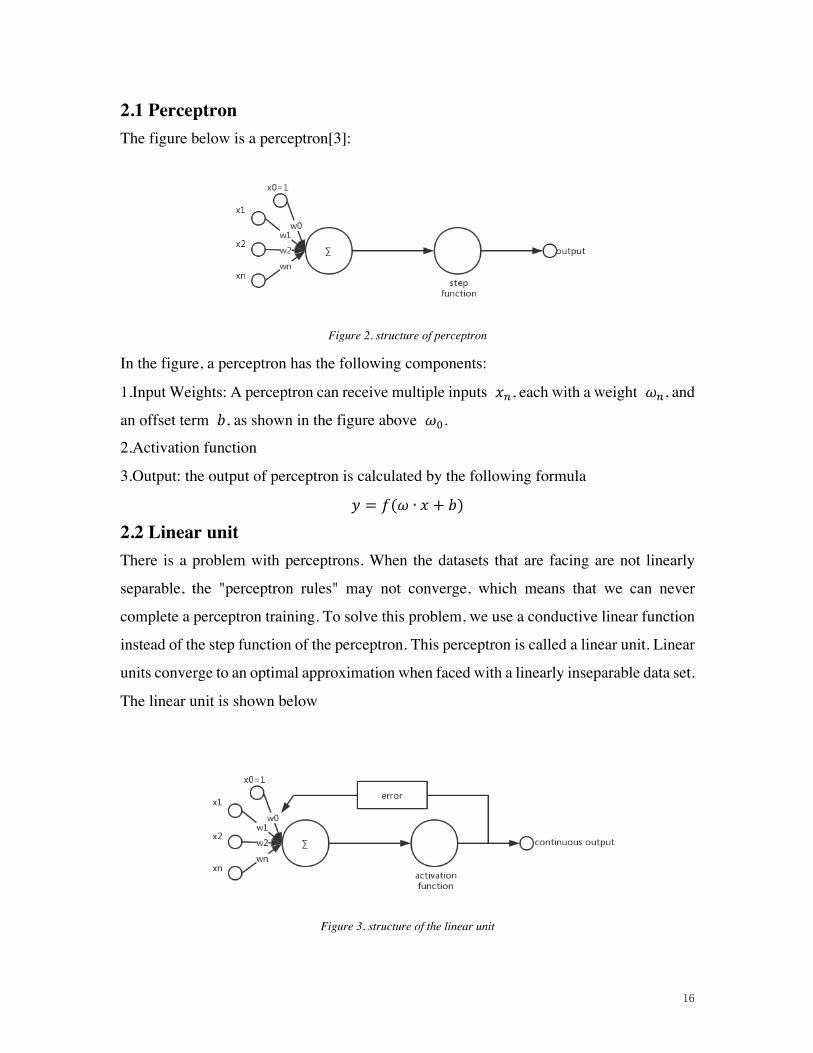
2.1 Perceptron The figure below is a perceptron[3]:

Figure 2. structure of perceptron

In the figure, a perceptron has the following components:

1.Input Weights: A perceptron can receive multiple inputs 𝑥&, each with a weight 𝜔&, and

an offset term 𝑏, as shown in the figure above 𝜔).

2.Activation function

3.Output: the output of perceptron is calculated by the following formula

𝑦 = 𝑓(𝜔 ∙ 𝑥 + 𝑏)

2.2 Linear unit There is a problem with perceptrons. When the datasets that are facing are not linearly

separable, the "perceptron rules" may not converge, which means that we can never

complete a perceptron training. To solve this problem, we use a conductive linear function

instead of the step function of the perceptron. This perceptron is called a linear unit. Linear

units converge to an optimal approximation when faced with a linearly inseparable data set.

The linear unit is shown below

Figure 3. structure of the linear unit

17

After replacing the activation function, the linear unit will return a real value instead of a

0,1 classification. Therefore linear units are used to solve regression problems rather than

classification problems.

2.3 Supervised learning and unsupervised learning Machine learning has a learning method called supervised learning[4]. It means that to train

a model, we need to provide a bunch of training samples: each training sample includes

both the input feature x and the corresponding output y. In other words, we have to find a

lot of people, we know their characteristics (working years, industry...) and know their

income. We use this sample to train the model so that the model sees each of our questions

(input feature x) and the answer to the corresponding question (true value 𝑦∗). When the

model sees enough samples, it can summarize some of these rules. Then, you can predict

the answer to the input that it has not seen.

Another type of learning method is called unsupervised learning[4]. The training sample

of this method has only x and no y. The model can summarize some rules of the feature x,

but can't know its corresponding answer 𝑦∗.

Many times, training samples with both x and y are rare, and most samples only have x.

For example, in speech-to-text (STT) recognition tasks, x is speech and 𝑦∗ is the text

corresponding to this speech. It's easy to get a lot of voice recordings, but it's very laborious

to split the voice into sections and mark the corresponding text. In this case, to compensate

for the shortage of labeled samples, we can use the unsupervised learning method to do

some clustering first, let the model summarize which syllables are similar, and then use a

small number of labeled training samples to tell the model. Some syllables correspond to

the text. In this way, the model can match similar syllables to the corresponding text and

complete the training of the model.

2.4 The objective function of a linear unit Under supervised learning, for a sample, we know its characteristic x and the true value

𝑦∗. At the same time, we can also calculate the output y based on the model h(x). Note

that we use 𝑦∗ to indicate the true value in the training sample, which is the actual value;

the 𝑦 indicates the predicted value calculated by the model. We certainly hope that the y

and 𝑦∗ calculated by the model are as close as possible.

18

There are many ways to express the closeness of y and 𝑦∗ in mathematics. For example,

we can use the square of the difference between y and 𝑦∗ to indicate their closeness.

𝑒 =12(𝑦∗ − 𝑦)7 (1)

We call𝑒 the error of a single sample. It is convenient for later calculation multiplied by

1/2.

If there are N samples in the training data, We can use the sum of the errors of all the

samples in the training data to represent the error E of the model, that is,

𝐸 = 𝑒: + 𝑒7 + 𝑒; + ⋯+ 𝑒& (2)

𝑒: of the above formula represents the error of the first sample, and 𝑒7 represents the

error of the second sample…

For convenience, we can also write the above formula as a summation formula.

𝐸 = 𝑒: + 𝑒7 + 𝑒; + ⋯+ 𝑒& (3)

=>𝑒?&

?@:

(4)

=12>

B𝑦∗(?) − 𝑦(?)C7&

?@:

(5)

Among them,

𝑦(?) = ℎB𝑥(?)C (6)

= wHx(J) (7)

x(J) represents the feature of the i-th training sample, 𝑦∗(?) represents the true value of the

i-th sample, and we can also use the tuple (x(J), 𝑦∗(?)) to represent the i-th training sample.

𝑦(?) is the predicted value of the model for the i-th sample.

For a training data set, the error needs to be as small as possible, which means the value in

the formula (5) need to be small. For a particular training data set, the values of (x(J), 𝑦∗(?))

are known, so formula (5) is a function of the parameters.

𝐸(w) =12>

B𝑦∗(?) − 𝑦(?)C7

&

?@:

(8)

19

=12>

B𝑦∗(?) − wHx(J)C7

&

?@:

(9)

The training of the model is actually to obtain the appropriate w, so that (Formula 5)

obtains the minimum value which is called the optimization problem in mathematics, and

𝐸(w) is the goal of our optimization, called the objective function.

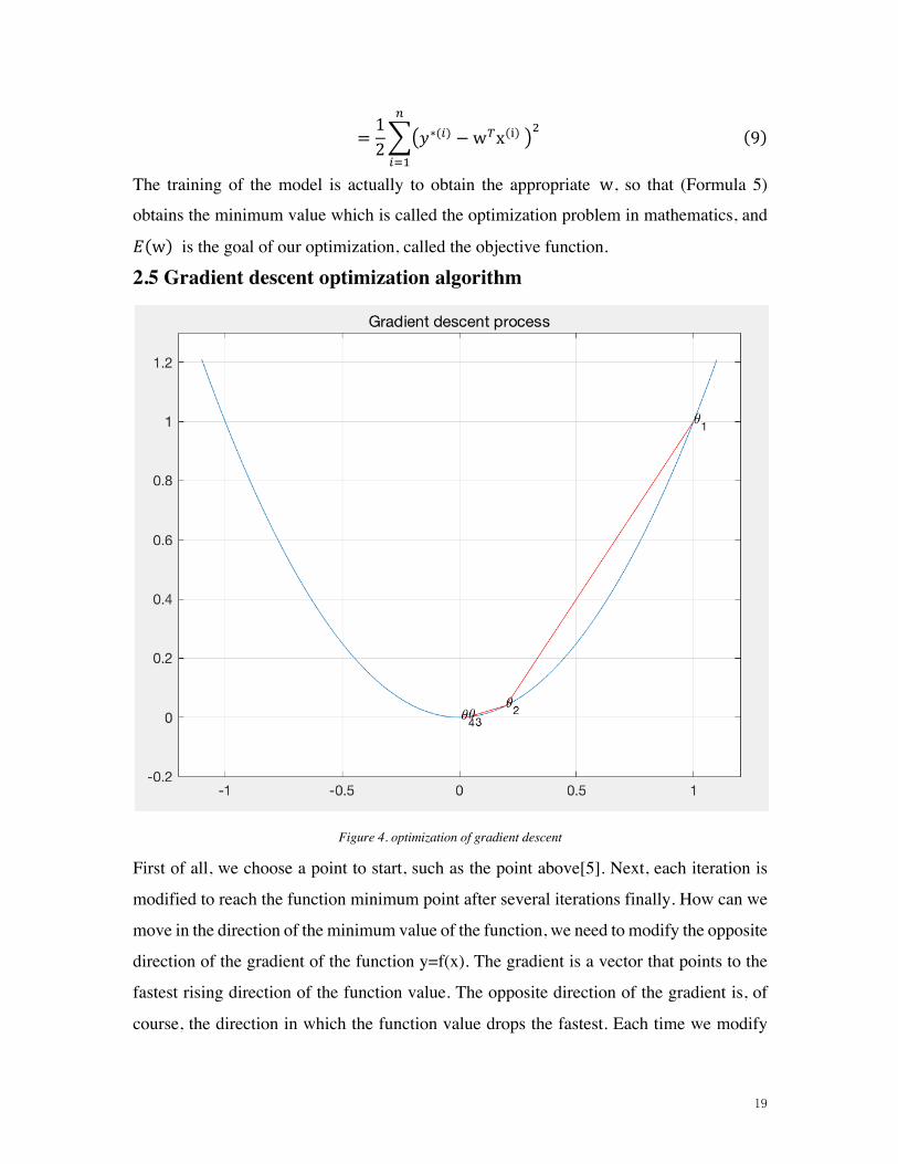
2.5 Gradient descent optimization algorithm

Figure 4. optimization of gradient descent

First of all, we choose a point to start, such as the point above[5]. Next, each iteration is

modified to reach the function minimum point after several iterations finally. How can we

move in the direction of the minimum value of the function, we need to modify the opposite

direction of the gradient of the function y=f(x). The gradient is a vector that points to the

fastest rising direction of the function value. The opposite direction of the gradient is, of

course, the direction in which the function value drops the fastest. Each time we modify

20

the value of x along the opposite direction of the gradient, we can, of course, go near the

minimum of the function(3).

According to the above discussion, we can write the formula of the gradient descent

algorithm.

wN = w − 𝜂∇𝑓(𝑥) (10)

From the formula (5)

𝐸(w) =12>

B𝑦∗(?) − 𝑦(?)C7

&

?@:

(11)

if we need the maximum value of the objective function, we should use the gradient ascent

algorithm, and its parameter modification rule is

wN = w + 𝜂∇𝑓(𝑥) (12)

The gradient of the objective function is

∇𝐸(w) = −>B𝑦∗(?) − 𝑦(?)Cx?&

?@:

(13)

Therefore, the parameter modification rule of the linear unit is finally like this

wN = w + 𝜂>B𝑦∗(?) − 𝑦(?)Cx?&

?@:

(14)

2.5.1 Derivation of ∇E(w)

We know that the definition of the gradient of a function is it is partial derivative relative

to each variable[5], so we write the following formula

∇𝐸(w) =𝜕𝜕w

𝐸(w) (15)

=𝜕𝜕w

12>

B𝑦∗(?) − 𝑦(?)C7

&

?@:

(16)

We know that the derivative of a sum is equal to the sum of the derivatives, so we can first

find the derivatives in the summation symbol Σ, and then add them together

𝜕𝜕w

12>

B𝑦∗(?) − 𝑦(?)C7

&

?@:

(17)

=12>

𝜕𝜕w

B𝑦∗(?) − 𝑦(?)C7&

?@:

(18)

21

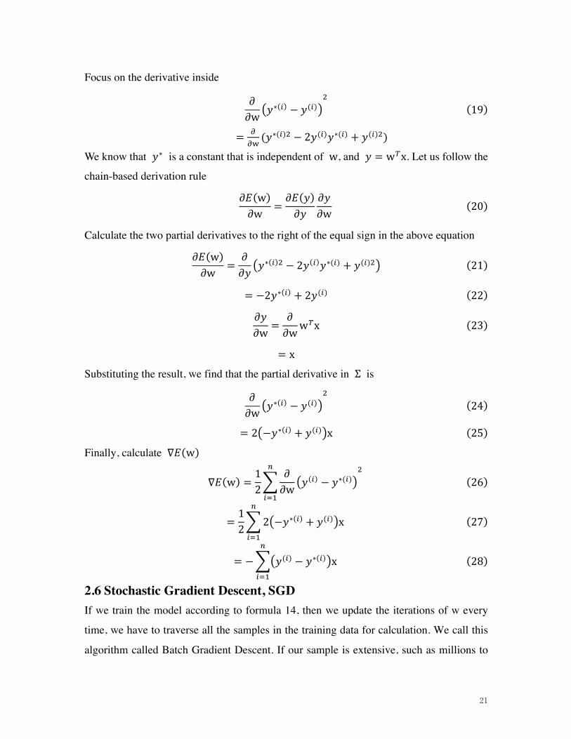
Focus on the derivative inside

𝜕𝜕w

B𝑦∗(?) − 𝑦(?)C7

(19)

= SST(𝑦∗(?)7 − 2𝑦(?)𝑦∗(?) + 𝑦(?)7)

We know that 𝑦∗ is a constant that is independent of w, and 𝑦 = wHx. Let us follow the

chain-based derivation rule

𝜕𝐸(w)𝜕w

=𝜕𝐸(𝑦)𝜕𝑦

𝜕𝑦𝜕w

(20)

Calculate the two partial derivatives to the right of the equal sign in the above equation

𝜕𝐸(w)𝜕w

=𝜕𝜕𝑦B𝑦∗(?)7 − 2𝑦(?)𝑦∗(?) + 𝑦(?)7C (21)

= −2𝑦∗(?) + 2𝑦(?) (22)

𝜕𝑦𝜕w

=𝜕𝜕w

wHx (23)

= x

Substituting the result, we find that the partial derivative in Σ is

𝜕𝜕w

B𝑦∗(?) − 𝑦(?)C7

(24)

= 2B−𝑦∗(?) + 𝑦(?)Cx (25)

Finally, calculate ∇𝐸(w)

∇𝐸(w) =12>

𝜕𝜕w

B𝑦(?) − 𝑦∗(?)C7&

?@:

(26)

=12>2B−𝑦∗(?) + 𝑦(?)Cx

&

?@:

(27)

= −>B𝑦(?) − 𝑦∗(?)Cx&

?@:

(28)

2.6 Stochastic Gradient Descent, SGD If we train the model according to formula 14, then we update the iterations of w every

time, we have to traverse all the samples in the training data for calculation. We call this

algorithm called Batch Gradient Descent. If our sample is extensive, such as millions to

22

hundreds of millions, then the amount of calculation is enormous. Therefore, a practical

algorithm is the SGD algorithm[6]. In the SGD algorithm, only calculate one sample each

time with the iteration of updated w. In this way, for training data with millions of samples,

a traversal will update millions of times, and the efficiency will be significantly improved.

Due to the noise and randomness of the sample, each update w does not necessarily follow

the direction of decreasing E. However, although there is some randomness, a large number

of updates generally progress in the direction of E reduction, and therefore can finally

converge to near the minimum. The figure below shows the difference between SGD and

BGD.

Figure 5. difference between SGD and BGD.

As shown above, ellipse represents the contour of the function value, and the center of

the ellipse is the minimum point of the function. Red is the approximation curve of BGD,

and purple is the approximation curve of SGD. We can see that BGD has been moving

towards the lowest point, and SGD has obviously moved a lot, but overall, it is still

approaching the lowest point.

We can see that SGD is not only efficient, but randomness is sometimes a good thing. The

objective function in the figure is a "convex function" that finds a globally unique minimum

along the opposite direction of the gradient. However, for non-convex functions, there are

many local minima. Randomness helps us escape some very bad local minima to get a

better model.

23

3 Artificial Neural Network Artificial Neural Network (ANN), referred to as Neural Network (NN) or neural network

in the field of machine learning and cognitive science, is a mimicking biological neural

network. In particular, mathematical models or computational models of the structure and

function of the brain used to estimate or approximate functions. The neural network is

calculated by a large number of artificial neuronal connections. In most cases, artificial

neural networks can change the internal structure based on external information. It is an

adaptive system. In general, it has a learning function. New neural networks are a kind of

non-linear statistical data modeling tools.

An artificial neural network (ANN) or a connected system is a computational system that

is ambiguously inspired by the biological neural network that makes up the animal's brain.

Neural networks are a combination of many different machine learning algorithms that

handle advanced complex data inputs rather than a single algorithm. This kind of system

goes through the sample to complete the task of learning, usually without any specific task

rules. For example, in image recognition, they may learn to identify images containing cats

as "cats" or "no cats" by analyzing manual sample images and use the advanced model to

identify the target in the test images, they do this without any basic knowledge about the

cat; for example, they have fur, tail, beard, and cat-like faces. Instead, they automatically

generate recognition features from the learning materials they process. The structure of an

original ANN is showed below.

24

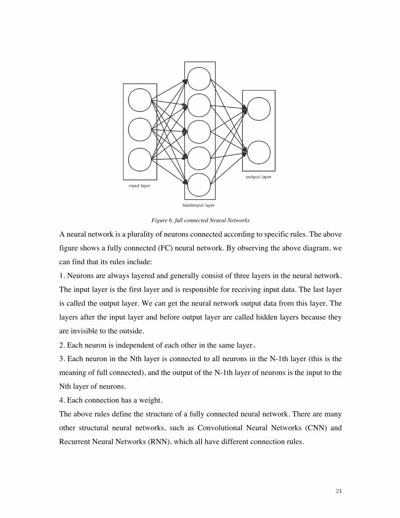
Figure 6. full connected Neural Networks

A neural network is a plurality of neurons connected according to specific rules. The above

figure shows a fully connected (FC) neural network. By observing the above diagram, we

can find that its rules include:

1. Neurons are always layered and generally consist of three layers in the neural network.

The input layer is the first layer and is responsible for receiving input data. The last layer

is called the output layer. We can get the neural network output data from this layer. The

layers after the input layer and before output layer are called hidden layers because they

are invisible to the outside.

2. Each neuron is independent of each other in the same layer。

3. Each neuron in the Nth layer is connected to all neurons in the N-1th layer (this is the

meaning of full connected), and the output of the N-1th layer of neurons is the input to the

Nth layer of neurons.

4. Each connection has a weight.

The above rules define the structure of a fully connected neural network. There are many

other structural neural networks, such as Convolutional Neural Networks (CNN) and

Recurrent Neural Networks (RNN), which all have different connection rules.

25

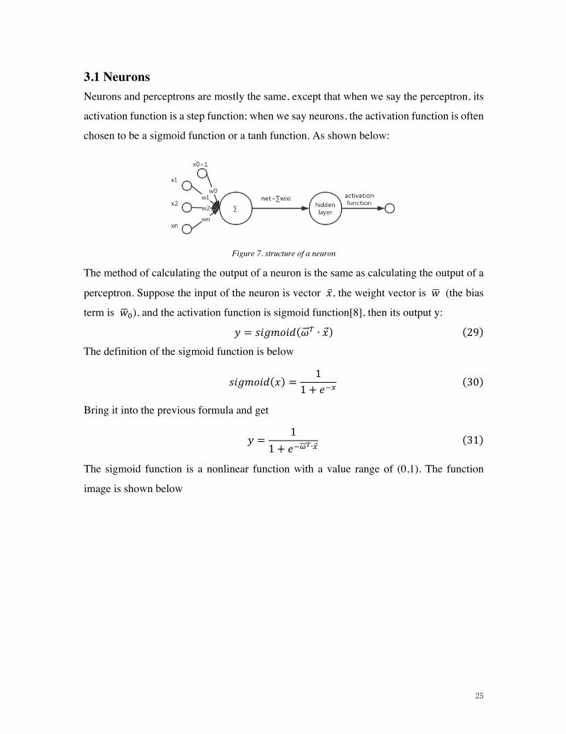
3.1 Neurons Neurons and perceptrons are mostly the same, except that when we say the perceptron, its

activation function is a step function; when we say neurons, the activation function is often

chosen to be a sigmoid function or a tanh function. As shown below:

Figure 7. structure of a neuron

The method of calculating the output of a neuron is the same as calculating the output of a

perceptron. Suppose the input of the neuron is vector �̅�, the weight vector is 𝑤W (the bias

term is 𝑤W)), and the activation function is sigmoid function[8], then its output y:

𝑦 = 𝑠𝑖𝑔𝑚𝑜𝑖𝑑(�̂⃗̂�H ∙ 𝑥) (29)

The definition of the sigmoid function is below

𝑠𝑖𝑔𝑚𝑜𝑖𝑑(𝑥) =1

1 + 𝑒`a(30)

Bring it into the previous formula and get

𝑦 =1

1 + 𝑒`b̂⃗̂̂c∙a⃗(31)

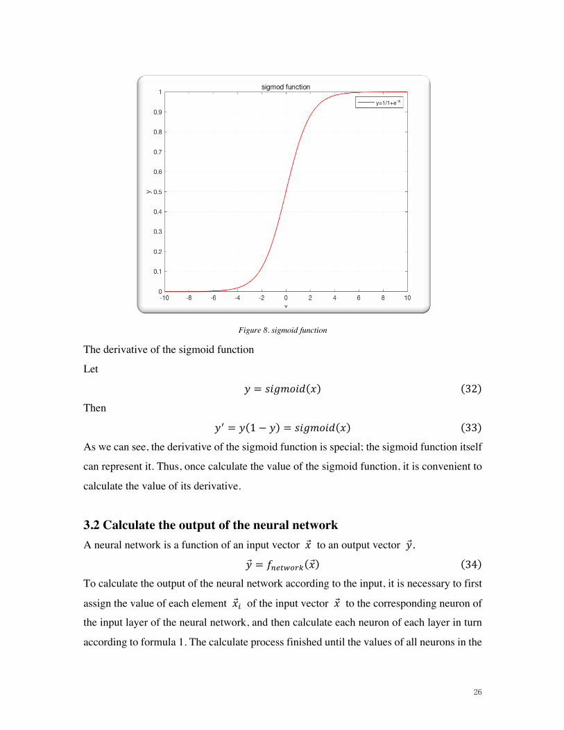
The sigmoid function is a nonlinear function with a value range of (0,1). The function

image is shown below

26

Figure 8. sigmoid function

The derivative of the sigmoid function

Let

𝑦 = 𝑠𝑖𝑔𝑚𝑜𝑖𝑑(𝑥) (32)

Then

𝑦N = 𝑦(1 − 𝑦) = 𝑠𝑖𝑔𝑚𝑜𝑖𝑑(𝑥) (33)

As we can see, the derivative of the sigmoid function is special; the sigmoid function itself

can represent it. Thus, once calculate the value of the sigmoid function, it is convenient to

calculate the value of its derivative.

3.2 Calculate the output of the neural network A neural network is a function of an input vector �⃗� to an output vector �⃗�,

�⃗� = 𝑓&defghi(�⃗�) (34)

To calculate the output of the neural network according to the input, it is necessary to first

assign the value of each element �⃗�? of the input vector �⃗� to the corresponding neuron of

the input layer of the neural network, and then calculate each neuron of each layer in turn

according to formula 1. The calculate process finished until the values of all neurons in the

27

last layer of the output layer are calculated. Finally, the output vector �⃗� is obtained by

stringing together the values of each neuron in the output layer.

Let's take an example to illustrate this process. First number each cell of the neural network.

Figure 9 neural network

As shown in the figure above, the input layer has three nodes, which we numbered as 1, 2,

and 3 in sequence; the four nodes in the hidden layer are numbered 4, 5, 6, and 7 in

sequence; the last two nodes in the output layer are number 8 and 9. Because our neural

network is fully connected, we can see that each node is connected to all nodes in the upper

layer. For example, we can see node 4 of the hidden layer, which is connected to the three

nodes 1, 2, and 3 of the input layer, and the weights on the connection are 𝜔j: 𝜔j7,𝜔j;

In order to calculate the output value of node 4, we must first obtain the output values of

all its upstream nodes (which are nodes 1, 2, 3). Nodes 1, 2, and 3 are nodes of the input

layer, so their output value is the input vector �⃗� itself. According to the corresponding

relationship in the above picture, the output values of nodes 1, 2, and 3 are𝑥:, 𝑥7and 𝑥;

respectively. We require that the dimensions of the input vector be the same as the number

of input layer neurons, and which input node of the input vector corresponds to which input

node is freely determinable.

28

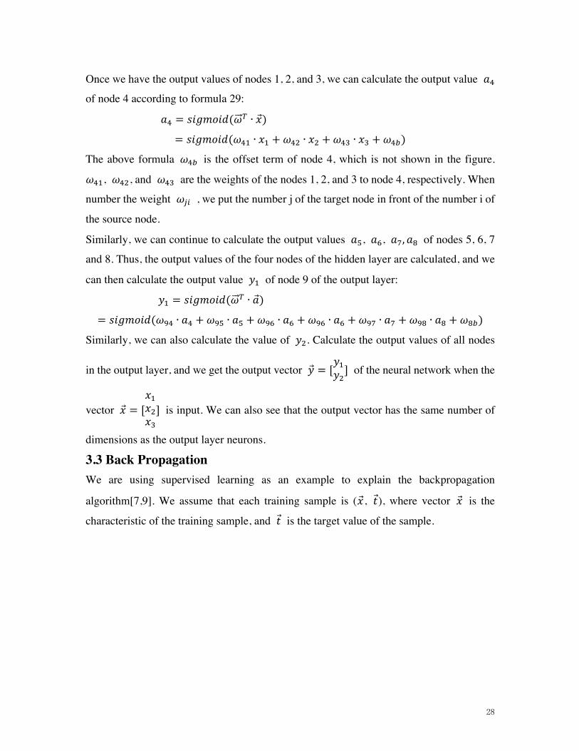
Once we have the output values of nodes 1, 2, and 3, we can calculate the output value 𝑎j

of node 4 according to formula 29:

𝑎j = 𝑠𝑖𝑔𝑚𝑜𝑖𝑑(�⃗̂̂�H ∙ �⃗�)

= 𝑠𝑖𝑔𝑚𝑜𝑖𝑑(𝜔j: ∙ 𝑥: + 𝜔j7 ∙ 𝑥7 + 𝜔j; ∙ 𝑥; + 𝜔jl)

The above formula 𝜔jl is the offset term of node 4, which is not shown in the figure.

𝜔j:, 𝜔j7, and 𝜔j; are the weights of the nodes 1, 2, and 3 to node 4, respectively. When

number the weight 𝜔m? , we put the number j of the target node in front of the number i of

the source node.

Similarly, we can continue to calculate the output values 𝑎n, 𝑎o, 𝑎p, 𝑎r of nodes 5, 6, 7

and 8. Thus, the output values of the four nodes of the hidden layer are calculated, and we

can then calculate the output value 𝑦: of node 9 of the output layer:

𝑦: = 𝑠𝑖𝑔𝑚𝑜𝑖𝑑(�̂⃗̂�H ∙ �⃗�)

= 𝑠𝑖𝑔𝑚𝑜𝑖𝑑(𝜔sj ∙ 𝑎j + 𝜔sn ∙ 𝑎n + 𝜔so ∙ 𝑎o + 𝜔so ∙ 𝑎o + 𝜔sp ∙ 𝑎p + 𝜔sr ∙ 𝑎r + 𝜔rl)

Similarly, we can also calculate the value of 𝑦7. Calculate the output values of all nodes

in the output layer, and we get the output vector �⃗� = [𝑦:𝑦7] of the neural network when the

vector �⃗� = [𝑥:𝑥7𝑥;] is input. We can also see that the output vector has the same number of

dimensions as the output layer neurons.

3.3 Back Propagation We are using supervised learning as an example to explain the backpropagation

algorithm[7,9]. We assume that each training sample is (𝑥, 𝑡), where vector �⃗� is the

characteristic of the training sample, and 𝑡 is the target value of the sample.

29

Figure 10. neural network

First, based on the algorithm introduced in the previous section, we use the feature �⃗� of

the sample to calculate the output 𝑎? of each hidden layer node in the neural network and

the output 𝑦? of each node in the output layer.[9]

Then, we calculate the error term 𝛿? of each node as below:

For output layer node 𝑖,

𝛿? = 𝑦?(1 − 𝑦?)(𝑡? − 𝑦?) (35)

Where 𝛿? is the error term of node 𝑖, 𝑦? is the output value of node𝑖, and 𝑡? is the target

value of the sample corresponding to node 𝑖. For example, according to the above figure,

for the output layer node 9, its output value is 𝑦:, and the target value of the sample is 𝑡:,

use the equation into the above gives the error term 𝛿s of the node 9 should be:

𝛿s = 𝑦:(1 − 𝑦:)(𝑡: − 𝑦:)

For hidden layer nodes[9],

𝛿? = 𝑎?(1 − 𝑎?) > 𝜔i?i∈gyezye{

𝛿i (36)

30

Where 𝑎? is the output value of node𝑖, 𝜔i?is the weight of the connection of the node

𝑖to its next layer node 𝑘, and 𝛿i is the error term of the node of the next layer of node

𝑘. For example, for hidden layer node 4, the calculation method is below:

𝛿j = 𝑎j(1 − 𝑎j)(𝜔sj𝛿s + 𝜔:),j𝛿:))

Finally, update the weights on each connection:

𝜔m? ← 𝜔m? + 𝜂𝛿m𝑥m? (37)

Where 𝜔m? is the weight of node𝑖 to node 𝑗, 𝜂 is a constant that becomes the learning

rate, 𝛿m is the error term of node 𝑗, and 𝑥m?is the input that node 𝑖 passes to node𝑗.

Obviously, to calculate the error term of a node, we need to calculate the error term of each

node that connects to this node. This requires that the order of the error terms must be

calculated from the output layer, and then calculate the error terms of each hidden layer

reversely, until the hidden layer connected to the input layer. This is the reason why we

called this algorithm of the backpropagation algorithm. When the error terms of all nodes

are calculated, we can update all the weights according to Equation 37.

3.4 Derivation of the backpropagation algorithm The backpropagation algorithm is the application of the chained derivation rule[9]. Next,

we use the chain derivation rule to derive the backpropagation algorithm, which is the

formula 35, 36, and 37 in the previous section.

According to the general routine of machine learning, we first determine the objective

function of the neural network and then use the stochastic gradient descent optimization

algorithm to find the parameter value at the minimum of the objective function.

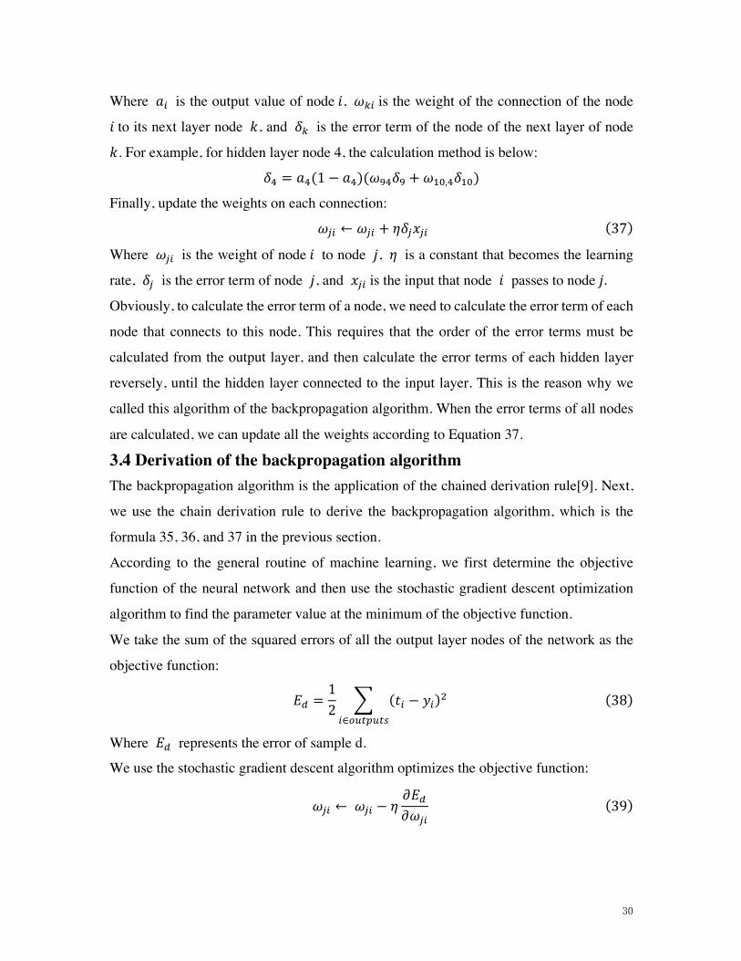
We take the sum of the squared errors of all the output layer nodes of the network as the

objective function:

𝐸� =12

> (𝑡? − 𝑦?)7?∈gyezye{

(38)

Where 𝐸� represents the error of sample d.

We use the stochastic gradient descent algorithm optimizes the objective function:

𝜔m? ← 𝜔m? − 𝜂𝜕𝐸�𝜕𝜔m?

(39)

31

The stochastic gradient descent algorithm also needs to find the partial derivative of the

error 𝐸� for each weight 𝜔m?

Figure 11. neural network

From the above figure, we find that the weight 𝜔m? can only affect other parts of the

network by affecting the input value of the node 𝑗. Let 𝑛𝑒𝑡mbe the weighted input of the

node 𝑗

𝑛𝑒𝑡m = �⃗̂̂�m ∙ �⃗�m (40)

=>𝜔m?𝑥m??

(41)

𝐸� is a function of 𝑛𝑒𝑡m, and 𝑛𝑒𝑡m is a function of 𝜔m?. According to the chain derivation

rule, we can get:

𝜕𝐸�𝜕𝜔m?

=𝜕𝐸�𝜕𝑛𝑒𝑡m

𝜕𝐸�𝜕𝑛𝑒𝑡m

(42)

=𝜕𝐸�𝜕𝑛𝑒𝑡m

𝜕 ∑ 𝜔m?𝑥m??

𝜕𝑛𝑒𝑡m(43)

=𝜕𝐸�𝜕𝑛𝑒𝑡m

𝑥m? (44)

32

In the above formula, 𝑥m? is the input value that node 𝑖 passes to node 𝑗, also is the output

value of node 𝑖.

For the derivation of S��S&de�

, it is necessary to distinguish between the output layer and the

hidden layer.

3.4.1 Output layer weight training

For the output layer, 𝑛𝑒𝑡m can only affect the rest of the network by the output value 𝑦m

of node 𝑗, that is, 𝐸� is a function of 𝑦m , and 𝑦m is a function of 𝑛𝑒𝑡m, where 𝑦m =

𝑠𝑖𝑚𝑜𝑖𝑑(𝑛𝑒𝑡m). So we can use the chain derivation rule again:

𝜕𝐸�𝜕𝑛𝑒𝑡m

=𝜕𝐸�𝜕𝑦m

𝜕𝑦m𝜕𝑛𝑒𝑡m

(45)

First part of the above formula:

𝜕𝐸�𝜕𝑦m

=𝜕𝜕𝑦?

12 > (𝑡? − 𝑦?)7?∈gyezye{

(46)

=𝜕𝜕𝑦?

12B𝑡m − 𝑦mC

7 (47)

= −B𝑡m − 𝑦mC (48)

Second part of the above formula:

𝜕𝑦m𝜕𝑛𝑒𝑡m

=𝜕𝑠𝑖𝑔𝑚𝑜𝑖𝑑B𝑛𝑒𝑡mC

𝜕𝑛𝑒𝑡m(49)

= 𝑦?B1 − 𝑦mC (50)

Bring the first and second part into the above formula:

𝜕𝐸�𝜕𝑛𝑒𝑡m

= −B𝑡m − 𝑦mC𝑦?B1 − 𝑦mC (51)

If 𝛿m = − S��S&de�

, that is the error term 𝛿 of a node is the inverse of the partial derivative of

the network error input to this node. Bring into the above formula, get

𝛿m = B𝑡m − 𝑦mC𝑦?B1 − 𝑦mC (52)

Which is the formula (35).

Bring the above derivation into the stochastic gradient descent formula to get:

33

𝜔m? ← 𝜔m? − 𝜂𝜕𝐸�𝜕𝜔m?

= 𝜔m? + 𝜂B𝑡m − 𝑦mC𝑦?B1 − 𝑦mC𝑥m? (53)

= 𝜔m? + 𝜂𝛿m𝑥m? (54)

Which is the formula (37)

3.4.2 Hidden layer weight training

Now we have to derive the S��S&de�

of the hidden layer.

First, we need to define a set 𝐷𝑜𝑤𝑛𝑠𝑡𝑟𝑒𝑎𝑚(𝑗) of all direct downstream nodes of the node

𝑗. For example, for node 4, its next downstream node is node 8, node 9. We can see that

𝑛𝑒𝑡m can only affect 𝐸� by affecting 𝐷𝑜𝑤𝑛𝑠𝑡𝑟𝑒𝑎𝑚(𝑗). Let 𝑛𝑒𝑡i be the input to the

downstream node of node 𝑗, then 𝐸� is a function of 𝑛𝑒𝑡i, and 𝑛𝑒𝑡i is a function of

𝑛𝑒𝑡m. Since there are multiple 𝑛𝑒𝑡is, we apply the full derivative formula and can make

the following derivation:

𝜕𝐸�𝜕𝑛𝑒𝑡m

= >𝜕𝐸�𝜕𝑛𝑒𝑡i

𝜕𝑛𝑒𝑡i𝜕𝑛𝑒𝑡mi∈�gf&{ehd��(m)

(55)

= > −𝛿i𝜕𝑛𝑒𝑡i𝜕𝑛𝑒𝑡mi∈�gf&{ehd��(m)

(56)

= > −𝛿i𝜕𝑛𝑒𝑡i𝜕𝑎m

𝜕𝑎m𝜕𝑛𝑒𝑡mi∈�gf&{ehd��(m)

(57)

= > −𝛿i𝜔im𝜕𝑎m𝜕𝑛𝑒𝑡mi∈�gf&{ehd��(m)

(58)

= > −𝛿i𝜔im𝑎mB1 − 𝑎mCi∈�gf&{ehd��(m)

(59)

= −𝑎mB1 − 𝑎mC > 𝛿i𝜔imi∈�gf&{ehd��(m)

(60)

Bring 𝛿m = − S��S&de�

to the above formula, get

𝛿m = B1 − 𝑎mC > 𝛿i𝜔imi∈�gf&{ehd��(m)

(61)

34

Which is formula 36

35

4 Recurrent Neural Network Some tasks need to be able to process the sequence information better, that is, the previous

input is related to the subsequent input. For example, when we understand the meaning of

a sentence, it is not enough to understand each word in isolation. We need to deal with the

whole sequence of these words. When we process the video, we cannot just go alone.

Analyze each frame and analyze the entire sequence of connections of these frames. At this

time, we need another significant neural network in the field of deep learning: Recurrent

Neural Network.

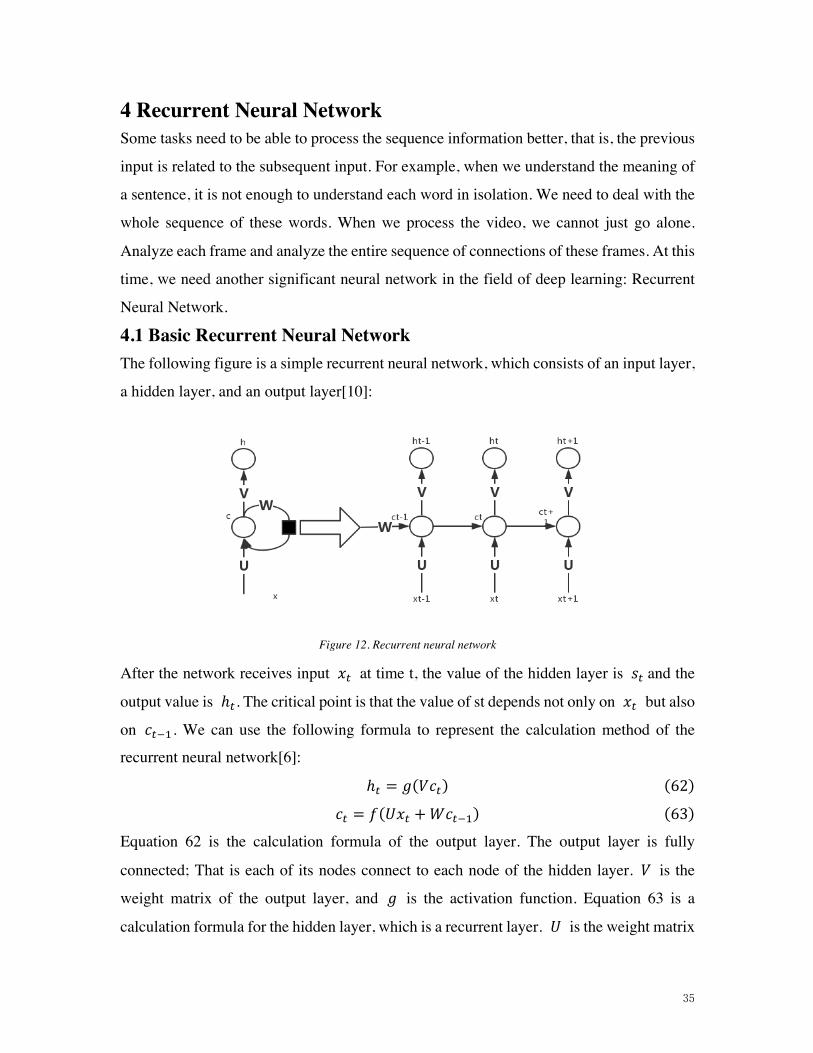
4.1 Basic Recurrent Neural Network The following figure is a simple recurrent neural network, which consists of an input layer,

a hidden layer, and an output layer[10]:

Figure 12. Recurrent neural network

After the network receives input 𝑥e at time t, the value of the hidden layer is 𝑠eand the

output value is ℎe. The critical point is that the value of st depends not only on 𝑥e but also

on 𝑐e`:. We can use the following formula to represent the calculation method of the

recurrent neural network[6]:

ℎe = 𝑔(𝑉𝑐e) (62)

𝑐e = 𝑓(𝑈𝑥e +𝑊𝑐e`:) (63)

Equation 62 is the calculation formula of the output layer. The output layer is fully

connected; That is each of its nodes connect to each node of the hidden layer. 𝑉 is the

weight matrix of the output layer, and 𝑔 is the activation function. Equation 63 is a

calculation formula for the hidden layer, which is a recurrent layer. 𝑈 is the weight matrix

36

of the input x, 𝑊 is the last value as the weight matrix for this input, and f is the

activation function.

If we repeatedly bring Equation 63 into Equation 62, we will get[7]:

ℎe = 𝑔(𝑉𝑐e) (64)

= 𝑉𝑓(𝑈𝑥e +𝑊𝑐e`:) (65)

= 𝑉𝑓B𝑈𝑥e +𝑊𝑓(𝑈𝑥e`: +𝑊𝑐e`7)C (66)

= 𝑉𝑓 �𝑈𝑥e +𝑊𝑓B𝑈𝑥e`: +𝑊𝑓(𝑈𝑥e`7 +𝑊𝑐e`;)C� (67)

= 𝑉𝑓 �𝑈𝑥e +𝑊𝑓 �𝑈𝑥e`: +𝑊𝑓B𝑈𝑥e`7 +𝑊𝑓(𝑈𝑥e`; + ⋯)C�� (68)

From the above, we know that the output value 𝑜e of the recurrent neural network is

affected by the previous input values 𝑥e, 𝑥e`:, 𝑥e`7, 𝑥e`;, ..., which is why the recurrent

neural network can look forward with any number of input values

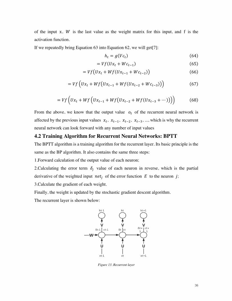
4.2 Training Algorithm for Recurrent Neural Networks: BPTT The BPTT algorithm is a training algorithm for the recurrent layer. Its basic principle is the

same as the BP algorithm. It also contains the same three steps:

1.Forward calculation of the output value of each neuron;

2.Calculating the error term 𝛿m value of each neuron in reverse, which is the partial

derivative of the weighted input 𝑛𝑒𝑡m of the error function 𝐸 to the neuron 𝑗;

3.Calculate the gradient of each weight.

Finally, the weight is updated by the stochastic gradient descent algorithm.

The recurrent layer is shown below:

Figure 13. Recurrent layer

37

1.Forward calculation

Forward calculation of the recurrent layer using formula 63:

𝑐e = 𝑓(𝑈𝑥e +𝑊𝑐e`:)

Note that the above 𝑐e, 𝑥e, and 𝑐e`: are vectors, which are represented by bold letters;

and U and V are matrices, which are represented by uppercase letters. The subscript of the

vector represents the time, for example, 𝑐e represents the value of the vector s at time t.

We assume that the dimension of the input vector x is m, the dimension of the output vector

c is n, then the dimension of the matrix U is 𝑛 × 𝑚, and the dimension of the matrix W is

𝑛 × 𝑛. Then we get the matrix from the above formula

⎣⎢⎢⎢⎡𝑐:e

𝑐7e∙∙𝑐&e ⎦⎥⎥⎥⎤= 𝑓

⎝

⎜⎛

⎣⎢⎢⎢⎡𝑢:: 𝑢:7 … 𝑢:�𝑢7: 𝑢77 … 𝑢7�

∙∙

𝑢&: 𝑢&7 … 𝑢&�⎦⎥⎥⎥⎤

⎣⎢⎢⎡𝑥:𝑥7∙∙𝑥�⎦⎥⎥⎤+

⎣⎢⎢⎢⎡𝜔:: 𝜔:7 … 𝜔:&𝜔7: 𝜔77 … 𝜔7&

∙∙

𝜔&: 𝜔&7 … 𝜔&&⎦⎥⎥⎥⎤

⎣⎢⎢⎢⎡𝑐:e`:

𝑐7e`:∙∙

𝑐&e`:⎦⎥⎥⎥⎤

⎠

⎟⎞

(69)

Here we use handwritten letters to represent an element of a vector, its subscript indicates

that it is the first element of the vector, and its superscript indicates the first few moments.

For example, 𝑐me represents the value of the 𝑗th element of the vector 𝑠 at time t. 𝑢m?

represents the weight of the 𝑖 -th neuron in the input layer to the 𝑗-th neuron in the

recurrent layer. 𝜔m? represents the weight of the 𝑖-th neuron at the 𝑡-1th point of the

recurrent layer to the 𝑗-th neuron at the tth moment of the recurrent layer.

2 Calculation of error terms

The BTPP algorithm propagates the error term 𝛿e£ value of the 𝑙 layer time 𝑡 in two

directions. One direction is that transmitted to the upper layer network to obtain 𝛿e£`:. This

part is only related to the weight matrix U; The other is that the direction is along its

timeline pass to the initial time 𝑡:, to get yields 𝛿:£ , which is only related to the weight

matrix𝑊.

We use the vector 𝑛𝑒𝑡e to represent the weighted input of the neuron at time t:

𝑛𝑒𝑡e = 𝑈𝑥e +𝑊𝑐e`: (70)

𝑐e`: = 𝑓(𝑛𝑒𝑡e`:) (71)

So

38

𝜕𝑛𝑒𝑡e𝜕𝑛𝑒𝑡e`:

=𝜕𝑛𝑒𝑡e𝜕𝑐e`:

𝜕𝑐e`:𝜕𝑛𝑒𝑡e`:

(72)

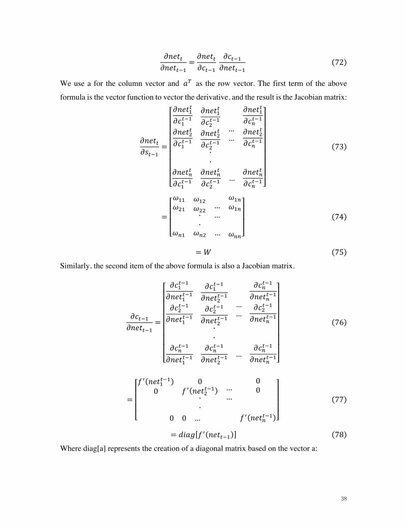
We use a for the column vector and 𝑎H as the row vector. The first term of the above

formula is the vector function to vector the derivative, and the result is the Jacobian matrix:

𝜕𝑛𝑒𝑡e𝜕𝑠e`:

=

⎣⎢⎢⎢⎢⎢⎢⎢⎡𝜕𝑛𝑒𝑡:

e

𝜕𝑐:e`:

𝜕𝑛𝑒𝑡7e

𝜕𝑐:e`:

𝜕𝑛𝑒𝑡:e

𝜕𝑐7e`:

𝜕𝑛𝑒𝑡7e

𝜕𝑐7e`:∙∙

……

𝜕𝑛𝑒𝑡:e

𝜕𝑐&e`:

𝜕𝑛𝑒𝑡7e

𝜕𝑐&e`:

𝜕𝑛𝑒𝑡&e

𝜕𝑐:e`:𝜕𝑛𝑒𝑡&e

𝜕𝑐7e`:…

𝜕𝑛𝑒𝑡&e

𝜕𝑐&e`: ⎦⎥⎥⎥⎥⎥⎥⎥⎤

(73)

=

⎣⎢⎢⎢⎡𝜔::𝜔7:

𝜔:7𝜔77∙∙

……

𝜔:&𝜔:&

𝜔&: 𝜔&7 … 𝜔&&⎦⎥⎥⎥⎤

(74)

= 𝑊 (75)

Similarly, the second item of the above formula is also a Jacobian matrix.

𝜕𝑐e`:𝜕𝑛𝑒𝑡e`:

=

⎣⎢⎢⎢⎢⎢⎢⎢⎡ 𝜕𝑐:

e`:

𝜕𝑛𝑒𝑡:e`:

𝜕𝑐7e`:

𝜕𝑛𝑒𝑡:e`:

𝜕𝑐:e`:

𝜕𝑛𝑒𝑡7e`:

𝜕𝑐7e`:

𝜕𝑛𝑒𝑡7e`:∙∙

……

𝜕𝑐&e`:

𝜕𝑛𝑒𝑡&e`:

𝜕𝑐7e`:

𝜕𝑛𝑒𝑡&e`:

𝜕𝑐&e`:

𝜕𝑛𝑒𝑡:e`:𝜕𝑐&e`:

𝜕𝑛𝑒𝑡7e`:…

𝜕𝑐&e`:

𝜕𝑛𝑒𝑡&e`:⎦⎥⎥⎥⎥⎥⎥⎥⎤

(76)

=

⎣⎢⎢⎢⎡𝑓

N(𝑛𝑒𝑡:e`:)0

0𝑓N(𝑛𝑒𝑡7e`:)

∙∙

……

00

0 0 … 𝑓N(𝑛𝑒𝑡&e`:)⎦⎥⎥⎥⎤

(77)

= 𝑑𝑖𝑎𝑔[𝑓N(𝑛𝑒𝑡e`:)] (78)

Where diag[a] represents the creation of a diagonal matrix based on the vector a:

39

𝑑𝑖𝑎𝑔(𝑎) =

⎣⎢⎢⎢⎡𝑎:0

0𝑎7∙∙

……

00

0 0 … 𝑎&⎦⎥⎥⎥⎤

(79)

Finally, combine the two items, we can get:

𝜕𝑛𝑒𝑡e𝜕𝑛𝑒𝑡e`:

=𝜕𝑛𝑒𝑡e𝜕𝑠e`:

𝜕𝑐e`:𝜕𝑛𝑒𝑡e`:

(80)

= 𝑊𝑑𝑖𝑎𝑔[𝑓N(𝑛𝑒𝑡e`:)] (81)

=

⎣⎢⎢⎢⎡𝜔::𝑓

N(𝑛𝑒𝑡:e`:)𝜔7:𝑓N(𝑛𝑒𝑡:e`:)

𝜔::𝑓N(𝑛𝑒𝑡7e`:)𝜔77𝑓N(𝑛𝑒𝑡7e`:)

∙∙

……

𝜔:&𝑓N(𝑛𝑒𝑡&e`:)𝜔7&𝑓N(𝑛𝑒𝑡&e`:)

𝜔&:𝑓N(𝑛𝑒𝑡:e`:) 𝜔&7𝑓N(𝑛𝑒𝑡7e`:) … 𝜔&&𝑓N(𝑛𝑒𝑡7e`:)⎦⎥⎥⎥⎤

(82)

The above formula describes the rule of passing 𝛿 a period forward along time. With

this rule, we can find the error term 𝛿i at any time k:

𝛿iH =𝜕𝐸𝜕𝑛𝑒𝑡i

(83)

=𝜕𝐸𝜕𝑛𝑒𝑡e

𝜕𝑛𝑒𝑡e𝜕𝑛𝑒𝑡i

(84)

=𝜕𝐸𝜕𝑛𝑒𝑡e

𝜕𝑛𝑒𝑡e𝜕𝑛𝑒𝑡e`:

𝜕𝑛𝑒𝑡e`:𝜕𝑛𝑒𝑡e`7

⋯𝜕𝑛𝑒𝑡i¥:𝜕𝑛𝑒𝑡i

(85)

= 𝑊𝑑𝑖𝑎𝑔[𝑓N(𝑛𝑒𝑡e`:)]𝑊𝑑𝑖𝑎𝑔[𝑓N(𝑛𝑒𝑡e`7)]⋯𝑊𝑑𝑖𝑎𝑔[𝑓N(𝑛𝑒𝑡i)]𝛿e£ (86)

= 𝛿eH¦𝑊𝑑𝑖𝑎𝑔[𝑓N(𝑛𝑒𝑡?)]e`:

?@i

(87)

formula 87 is an algorithm that propagates the error term back in time. The recurrent layer

passes the error term back to the upper layer network, which is the same as the standard

full connection layer.

The weighted input 𝑛𝑒𝑡£ of the recurrent layer is related to the weighted input 𝑛𝑒𝑡£`: of

the previous layer as follows

𝑛𝑒𝑡e£ = 𝑈𝑎e£`: +𝑊𝑐e`: (88)

𝑎e£`: = 𝑓£`:B𝑛𝑒𝑡e£`:C (89)

40

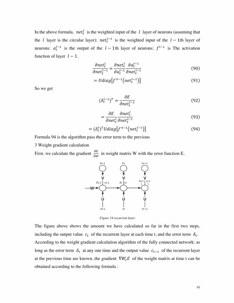
In the above formula, 𝑛𝑒𝑡e£ is the weighted input of the 𝑙 layer of neurons (assuming that

the 𝑙 layer is the circular layer); 𝑛𝑒𝑡e£`: is the weighted input of the 𝑙 − 1th layer of

neurons; 𝑎e£`: is the output of the 𝑙 − 1 th layer of neurons; 𝑓£`: is The activation

function of layer 𝑙 − 1.

𝜕𝑛𝑒𝑡e£

𝜕𝑛𝑒𝑡e£`:=𝜕𝑛𝑒𝑡e£

𝜕𝑎e£`:𝜕𝑎e£`:

𝜕𝑛𝑒𝑡e£`:(90)

= 𝑈𝑑𝑖𝑎𝑔§𝑓N£`:B𝑛𝑒𝑡e£`:C¨ (91)

So we get

(𝛿e£`:)H =𝜕𝐸

𝜕𝑛𝑒𝑡e£`:(92)

=𝜕𝐸𝜕𝑛𝑒𝑡e£

𝜕𝑛𝑒𝑡e£

𝜕𝑛𝑒𝑡e£`:(93)

= (𝛿e£)H𝑈𝑑𝑖𝑎𝑔§𝑓N£`:B𝑛𝑒𝑡e£`:C¨ (94)

Formula 94 is the algorithm pass the error term to the previous

3 Weight gradient calculation

First, we calculate the gradient S�S©

in weight matrix W with the error function E.

Figure 14 recurrent layer

The figure above shows the amount we have calculated so far in the first two steps,

including the output value 𝑐e of the recurrent layer at each time t, and the error term 𝛿e.

According to the weight gradient calculation algorithm of the fully connected network: as

long as the error term 𝛿e at any one time and the output value 𝑐e`: of the recurrent layer

at the previous time are known, the gradient ∇𝑊e𝐸 of the weight matrix at time t can be

obtained according to the following formula :

41

∇©ª𝐸 =

⎣⎢⎢⎢⎡𝛿:e𝑐:e`:

𝛿7e𝑐:e`:∙∙

𝛿:e𝑐7e`:

𝛿7e𝑐7e`:……

𝛿:e𝑐&e`:

𝛿7e𝑐&e`:

𝛿&e𝑐:e`: 𝛿&e𝑐7e`: … 𝛿&e𝑐&e`:⎦⎥⎥⎥⎤

(95)

In formula 95, 𝛿?e represents the 𝑖 component of the error term vector at time t;

𝑐?e`:represents the output value of the 𝑖 neuron in the cyclic layer at time 𝑡 − 1. Then we

carry out the derivation of formula 95

.

𝑛𝑒𝑡e = 𝑈𝑥e +𝑊𝑐e`: (96)

⎣⎢⎢⎢⎡𝑛𝑒𝑡:

e

𝑛𝑒𝑡7e∙∙

𝑛𝑒𝑡&e ⎦⎥⎥⎥⎤= 𝑈𝑥e +

⎣⎢⎢⎢⎡𝜔:: 𝜔:7 … 𝜔:&𝜔7: 𝜔77 … 𝜔7&

∙∙

𝜔&: 𝜔&7 … 𝜔&&⎦⎥⎥⎥⎤

⎣⎢⎢⎢⎡𝑐:e`:

𝑐7e`:∙∙

𝑐&e`:⎦⎥⎥⎥⎤

(97)

= 𝑈𝑥e +

⎣⎢⎢⎢⎡𝜔::𝑐:

e`: + 𝜔:7𝑐7e`: ⋯𝜔:&𝑐&e`:

𝜔7:𝑐:e`: + 𝜔77𝑐7e`: ⋯𝜔7&𝑐&e`:∙∙

𝜔&:𝑐:e`: + 𝜔&7𝑐7e`: ⋯𝜔&&𝑐&e`:⎦⎥⎥⎥⎤

(98)

Because the derivation of W has nothing to do with 𝑈𝑥e, so we ignore it. Now we consider

the weighting term 𝜔m? . By observing the above formula, we can see that 𝜔m? is only

related to 𝑛𝑒𝑡me, so:

𝜕𝐸𝜕𝜔m?

=𝜕𝐸𝜕𝑛𝑒𝑡me

𝜕𝑛𝑒𝑡me

𝜕𝜔m?(99)

= 𝛿me𝑐?e`: (100)

From the rule in formula 100, we can get formula 95

We have obtained the gradient ∇©ª𝐸 of the weight matrix W at time t, and the total

gradient ∇©𝐸 is the sum of the gradients at each moment.

∇©𝐸 =>∇©«𝐸e

?@:

(101)

42

=

⎣⎢⎢⎢⎡𝛿:e𝑐:e`:

𝛿7e𝑐:e`:∙∙

𝛿:e𝑐7e`:

𝛿7e𝑐7e`:……

𝛿:e𝑐&e`:

𝛿7e𝑐&e`:

𝛿&e𝑐:e`: 𝛿&e𝑐7e`: … 𝛿&e𝑐&e`:⎦⎥⎥⎥⎤

+ ⋯+

⎣⎢⎢⎢⎡𝛿:e𝑐:)

𝛿7e𝑐:)∙∙

𝛿:e𝑐7)

𝛿7e𝑐7)……

𝛿:e𝑐&)

𝛿7e𝑐&)

𝛿&e𝑐:) 𝛿&e𝑐7) … 𝛿&e𝑐&)⎦⎥⎥⎥⎤

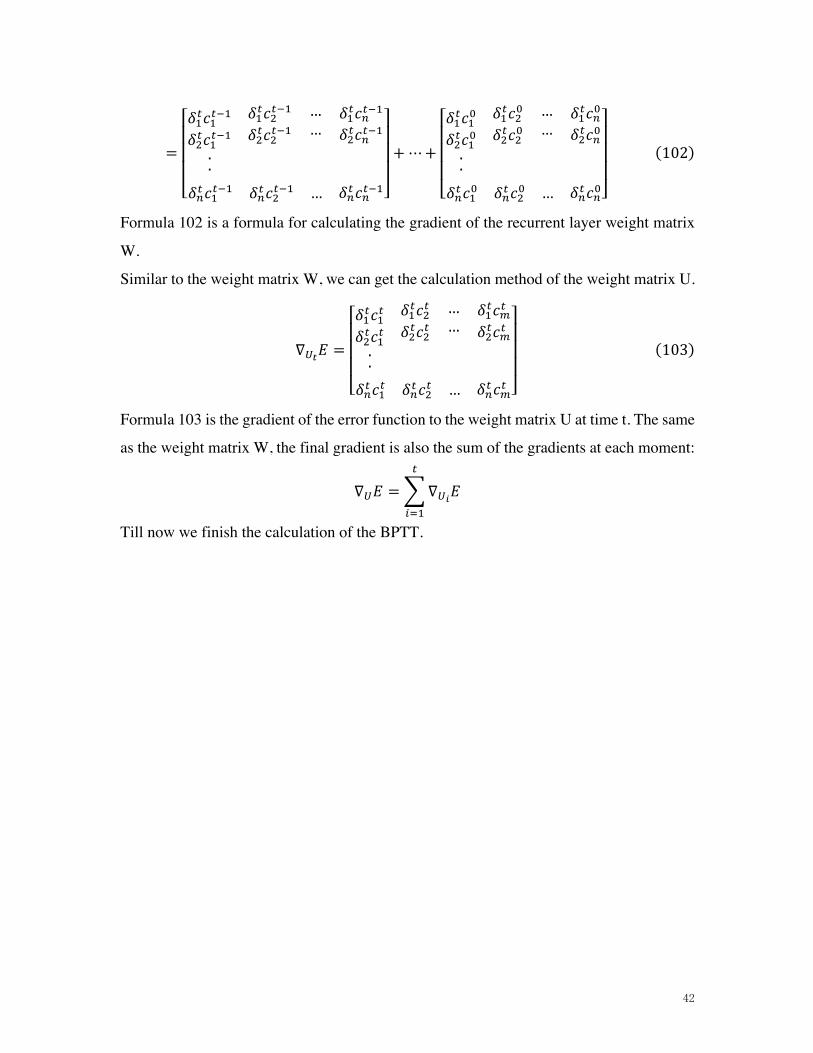
(102)

Formula 102 is a formula for calculating the gradient of the recurrent layer weight matrix

W.

Similar to the weight matrix W, we can get the calculation method of the weight matrix U.

∇¬ª𝐸 =

⎣⎢⎢⎢⎡𝛿:

e𝑐:e

𝛿7e𝑐:e∙∙

𝛿:e𝑐7e

𝛿7e𝑐7e……

𝛿:e𝑐�e

𝛿7e𝑐�e

𝛿&e𝑐:e 𝛿&e𝑐7e … 𝛿&e𝑐�e ⎦⎥⎥⎥⎤

(103)

Formula 103 is the gradient of the error function to the weight matrix U at time t. The same

as the weight matrix W, the final gradient is also the sum of the gradients at each moment:

∇¬𝐸 =>∇¬«𝐸e

?@:

Till now we finish the calculation of the BPTT.

43

5 Long Short-Term Memory Algorithm Long Short-Term Memory Algorithm (LSTM), which successfully solves the defects of

the original cyclic neural network, has become the most popular RNN and has been

successfully applied in many fields such as speech recognition, picture description, and

natural language processing.

Among them, it is an important reason to be able to deal with gradient explosions and

gradient hours that occur in ordinary RNN. From the last section, we know that The

formula for the error term to propagate back in time:

𝛿iH = 𝛿eH¦𝑊𝑑𝑖𝑎𝑔[𝑓N(𝑛𝑒𝑡?)]e`:

?@i

(104)

We can get the upper bound of the modulus of 𝛿iH according to the inequality below (the

modulo is a measure of the size of each value in 𝛿iH):

‖𝛿iH‖ ≤∥ 𝛿iH ∥¦ ∥e`:

?@i

𝑑𝑖𝑎𝑔[𝑓N(𝑛𝑒𝑡?)] ∥∥ 𝑊 ∥ (105)

≤∥ 𝛿iH ∥ B𝛽±𝛽©Ce`i (106)

We can see that the error term 𝛿 passed from time t to time k, and the upper bound of its

value is an exponential function of 𝛽±𝛽© . 𝛽±𝛽© is the upper bound of the diagonal

matrix𝑑𝑖𝑎𝑔[𝑓N(𝑛𝑒𝑡?)and the matrix W absolute value, respectively. Obviously, unless the

value of the product 𝛽±𝛽© is around 1, when the t-k is large (that is, when the error

transmitted for many times), the value of the whole expression becomes extremely small

(when the 𝛽±𝛽© product is less than 1) or (When the 𝛽±𝛽© product is greater than 1),

the former is the gradient disappears, and the latter is the gradient explosion[11].

In general, gradient explosions are easier to handle. Our program will receive a NaN error

when the gradient explodes. We can also set a gradient threshold that can be intercepted

directly when the gradient exceeds this threshold.

Thevanishinggradientismorechallengingtodetectandmoredifficulttohandle. We

have proved that the final gradient of the weighted array W is the sum of the gradients at

each moment. When the vanishing gradient, starting from this time t and going

forward,theresultinggradient(almostzero)willnotcontributetothefinalgradient

value,whichisequivalenttowhatthenetworkstatehisbeforethetimet,Intraining,

44

itwillnotaffecttheupdateoftheweightarrayW,thatis,thenetworkhasactually

ignoredthestatebeforethetimet.

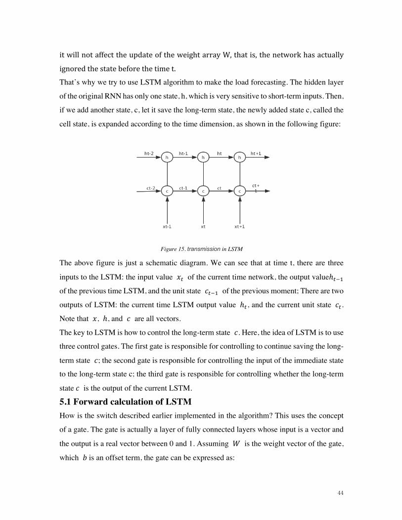
That’s why we try to use LSTM algorithm to make the load forecasting. The hidden layer

of the original RNN has only one state, h, which is very sensitive to short-term inputs. Then,

if we add another state, c, let it save the long-term state, the newly added state c, called the

cell state, is expanded according to the time dimension, as shown in the following figure:

Figure 15. transmission in LSTM

The above figure is just a schematic diagram. We can see that at time t, there are three

inputs to the LSTM: the input value 𝑥e of the current time network, the output valueℎe`:

of the previous time LSTM, and the unit state 𝑐e`: of the previous moment; There are two

outputs of LSTM: the current time LSTM output value ℎe, and the current unit state 𝑐e.

Note that 𝑥, ℎ, and 𝑐 are all vectors.

The key to LSTM is how to control the long-term state 𝑐. Here, the idea of LSTM is to use

three control gates. The first gate is responsible for controlling to continue saving the long-

term state 𝑐; the second gate is responsible for controlling the input of the immediate state

to the long-term state c; the third gate is responsible for controlling whether the long-term

state𝑐 is the output of the current LSTM.

5.1 Forward calculation of LSTM How is the switch described earlier implemented in the algorithm? This uses the concept

of a gate. The gate is actually a layer of fully connected layers whose input is a vector and

the output is a real vector between 0 and 1. Assuming 𝑊 is the weight vector of the gate,

which 𝑏is an offset term, the gate can be expressed as:

45

𝑔(𝑥) = 𝜎(𝑊a + 𝑏) (107)

The use of the gate is to multiply the element's output vector by the vector we want to

control. Since the output of the gate is a real vector between 0 and 1, then when the gate

output is 0, any vector multiplied will result in a 0 vector, which is equivalent to nothing

can pass; when the output is 1, any vector There is no change in multiplication, which is

equivalent to passing. Since the value range of x (the sigmoid function) is (0, 1), the state

of the gate is half-open and half-closed.

The LSTM uses two gates to control the contents of the unit state 𝑐. One is the forget gate,

which determines how much the unit state of 𝑐e`: is retained to the current time 𝑐e at the

previous time; The other is the input gate, it determines how much the input 𝑥e of the

network is saved to the unit state 𝑐e at the current moment. The LSTM uses an output gate

to control how much of the unit state 𝑐e is output to the current output value ℎe of the

LSTM.

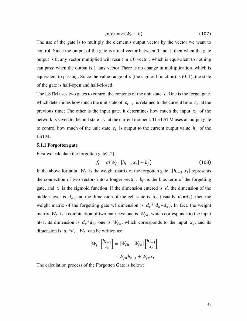
5.1.1 Forgotten gate

First we calculate the forgotten gate[12]:

𝑓e = 𝜎B𝑊± ∙ [ℎe`:, 𝑥e] + 𝑏±C (108)

In the above formula, 𝑊± is the weight matrix of the forgotten gate, [ℎe`:, 𝑥e]represents

the connection of two vectors into a longer vector, 𝑏± is the bias term of the forgetting

gate, and 𝑥 is the sigmoid function. If the dimension entered is 𝑑, the dimension of the

hidden layer is 𝑑Ë, and the dimension of the cell state is 𝑑Ì (usually 𝑑Ì=𝑑Ë), then the

weight matrix of the forgetting gate wf dimension is 𝑑Ì*(𝑑Ë+𝑑a ). In fact, the weight

matrix 𝑊± is a combination of two matrices: one is 𝑊±Ë, which corresponds to the input

ht-1, its dimension is 𝑑Ì*𝑑Ë ; one is 𝑊±a , which corresponds to the input 𝑥e , and its

dimension is 𝑑Ì*𝑑a. 𝑊± can be written as:

§𝑊±¨ Íℎe`:𝑥e

Î = [𝑊±Ë 𝑊±a] Íℎe`:𝑥e

Î

= 𝑊±Ëℎe`: +𝑊±a𝑥e

The calculation process of the Forgotten Gate is below:

46

Figure 16. calculation of the Forgotten gate

5.1.2 Input gate

Then let us see the input gate[12]

𝑖e = 𝜎(𝑊? ∙ [ℎe`:, 𝑥e] + 𝑏?) (109)

In the above formula, 𝑊? is the weight matrix of the input gate, 𝑏? is the offset term of

the input gate. The calculation process of the Forgotten Gate input gate is below:

Figure 17. calculation of 𝑖e in the Input gate

47

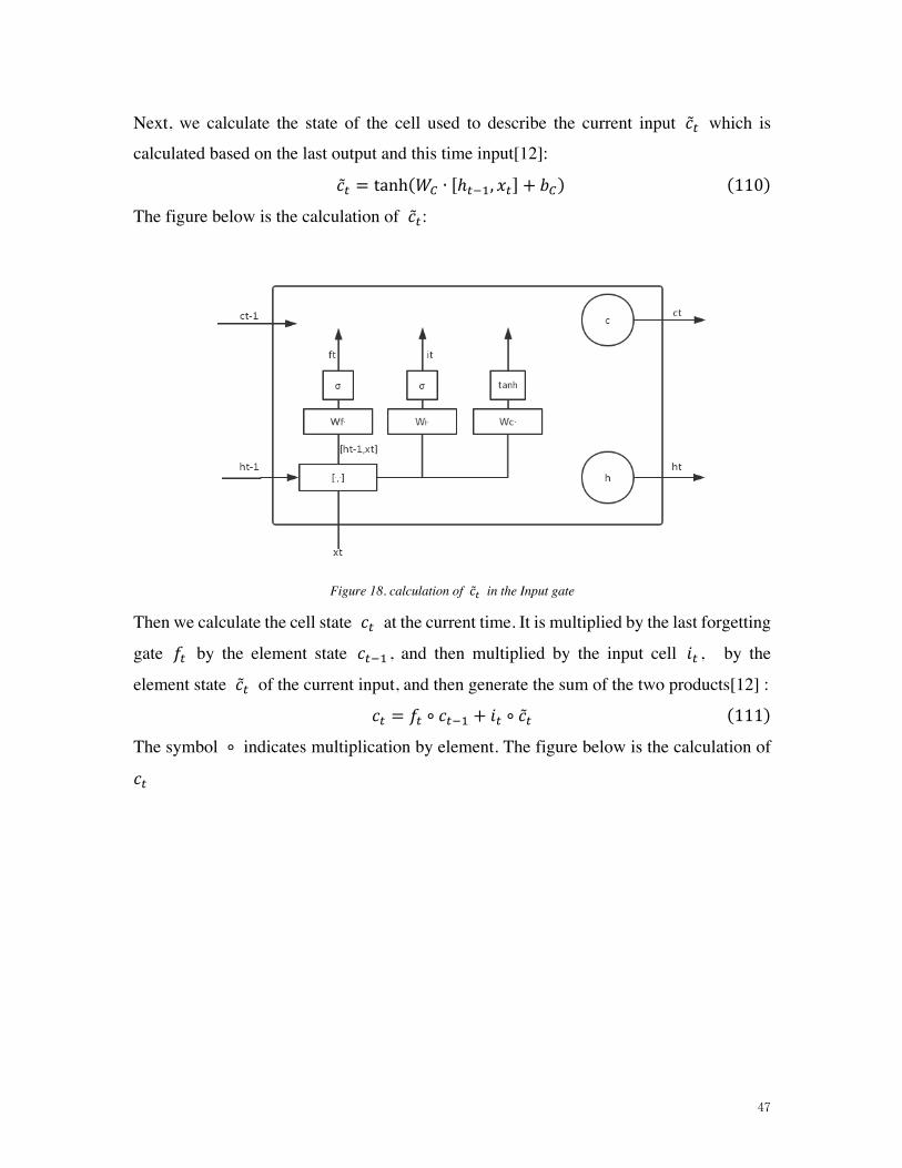
Next, we calculate the state of the cell used to describe the current input �̃�e which is

calculated based on the last output and this time input[12]:

�̃�e = tanh(𝑊Ð ∙ [ℎe`:, 𝑥e] + 𝑏Ð) (110)

The figure below is the calculation of �̃�e:

Figure 18. calculation of �̃�e in the Input gate

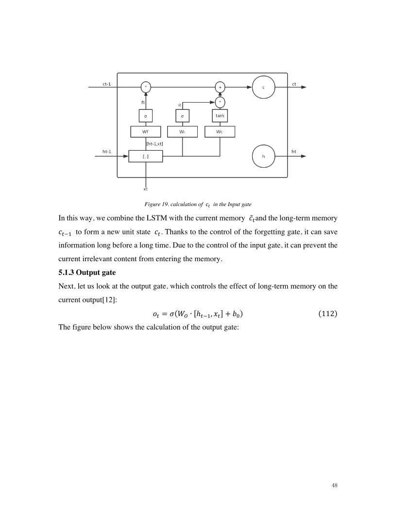
Then we calculate the cell state 𝑐e at the current time. It is multiplied by the last forgetting

gate 𝑓e by the element state 𝑐e`: , and then multiplied by the input cell 𝑖e , by the

element state �̃�e of the current input, and then generate the sum of the two products[12] :

𝑐e = 𝑓e ∘ 𝑐e`: + 𝑖e ∘ �̃�e (111)

The symbol ∘ indicates multiplication by element. The figure below is the calculation of

𝑐e

48

Figure 19. calculation of 𝑐e in the Input gate

In this way, we combine the LSTM with the current memory �̃�eand the long-term memory

𝑐e`: to form a new unit state 𝑐e. Thanks to the control of the forgetting gate, it can save

information long before a long time. Due to the control of the input gate, it can prevent the

current irrelevant content from entering the memory.

5.1.3 Output gate

Next, let us look at the output gate, which controls the effect of long-term memory on the

current output[12]:

𝑜e = 𝜎(𝑊Ò ∙ [ℎe`:, 𝑥e] + 𝑏)) (112)

The figure below shows the calculation of the output gate:

49

Figure 20. calculation of the output gate

The final output of the LSTM is determined by the output gate and the unit state:

ℎe = 𝑜e ∘ tanh(𝑐e) (113)

5.1.4 Final output

The figure below shows the calculation of the final output of the LSTM:

Figure 21. calculation of the final output

Till now, we have finished the LSTM forward calculation.

50

6 Training of the LSTM Framework of LSTM training algorithm[13]：

The training algorithm of LSTM is still a backpropagation algorithm, which has the

following three steps:

1.The output value of each neuron is Forward Propagation, for LSTM, that is, the five

vectors of values 𝑓e,𝑖e 𝑐e,𝑜e andℎe. The calculation method has been described in the

previous section.

2.Calculate the error term value𝛿 for each neuron in reverse. Like the recurrent neural

network, the backpropagation of the LSTM error term also includes two directions: one is

the backpropagation along time: from the current 𝑡 time, calculate the error term at each

moment; The other is to move the error term up one layer.

3.Calculated the gradient of each weight based on the corresponding error term.

There are eight groups of parameters that LSTM needs to learn, which are: the weight

matrix 𝑊± and bias term 𝑏± of the forgetting gate, the weight matrix 𝑊? and bias term

𝑏? of the input gate, the weight matrix 𝑊g and bias term 𝑏g of the output gate, and the

weight matrix𝑊Ì of the state of the computing unit and offset item 𝑏Ì.

6.1 Training process of LSTM in Matlab When training networks for deep learning, it is often useful to monitor the training progress.

By plotting various metrics during training, we can learn how the training is progressing.

For example, We can see if the accuracy of the training network is rising and whether the

network is overfit the training data by the training process.

When choosing to specify 'training-progress' as the 'Plots' value in training options and start

network training, train network draw a chart to show the changes in parameters for each

iteration of the training, each iteration is to update the gradients and weights in the model.

In regression networks, Matlab plots the root mean square error (RMSE) but not the

accuracy[13,15]. We choose the Stochastic Gradient Descent with Momentum(SGDM) to

training my data.

Gradient descent is a first-order iterative optimization algorithm used to find the minimum

value of a function. In order to ensure that the local minimum of the function can be found,

51

we need to calculate the step size opposite to the current function gradient. The options for

the training process are listed below[16]:

6.1.1 Initial Weights and Biases

In the matlab, the default initial weights is a 0 mean and standard deviation of 0.01 of a

gaussian distribution. The default for the initial bias value is 0. 1 choose the default value

in the training process.

6.1.2 Initial learning rate

Initial learning rate used for training.this parameter has a heavyweight of effecting the

training process. If we choose a value too low, then training takes a long time. If choose is

too high, then training might reach a suboptimal result or diverge. Most of the learning rate

is between 0.1-0.001. Choose the value between them and try to find the best value which

can get the lowest loss function in the training process.

6.2 Training process results By default, the training network uses this initial learning rate throughout the entire training

process. I choose to modify the learning rate every specified number of epochs by

multiplying the learning rate with a factor. Instead of using a low, fixed learning rate

throughout the training process, I choose a more significant learning rate at the beginning

of training and gradually reduce this value during optimization. Doing so can shorten the

training time while enabling smaller steps towards the minimum of the loss as training

progresses.

Set the other options in the training process as constant:

Minibatchsize:150

Maxexpoches:150

Gradient threshold:1

Learn rate drop period:100

Learn rate drop factor:0.2

Change the initial learning rate to find the best training parameter to get the lowest RMSE

and Loss.

Show the figure which uses different initial learning rate with 0.1,0.01,0.001 below

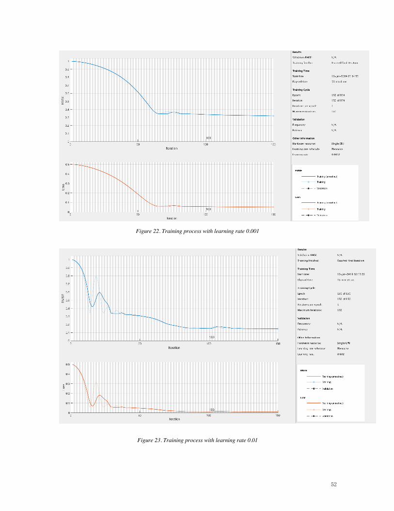
52

Figure 22. Training process with learning rate 0.001

Figure 23. Training process with learning rate 0.01

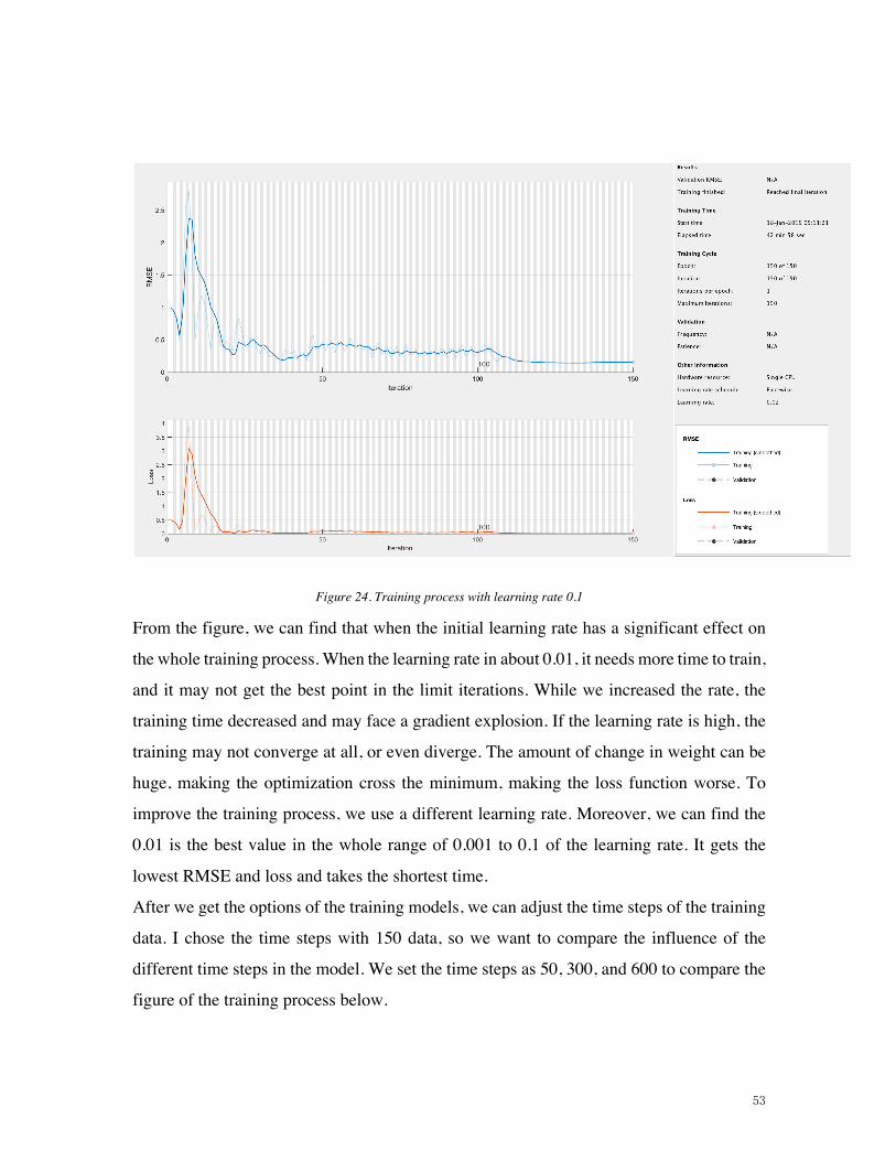
53

Figure 24. Training process with learning rate 0.1

From the figure, we can find that when the initial learning rate has a significant effect on

the whole training process. When the learning rate in about 0.01, it needs more time to train,

and it may not get the best point in the limit iterations. While we increased the rate, the

training time decreased and may face a gradient explosion. If the learning rate is high, the

training may not converge at all, or even diverge. The amount of change in weight can be

huge, making the optimization cross the minimum, making the loss function worse. To

improve the training process, we use a different learning rate. Moreover, we can find the

0.01 is the best value in the whole range of 0.001 to 0.1 of the learning rate. It gets the

lowest RMSE and loss and takes the shortest time.

After we get the options of the training models, we can adjust the time steps of the training

data. I chose the time steps with 150 data, so we want to compare the influence of the

different time steps in the model. We set the time steps as 50, 300, and 600 to compare the

figure of the training process below.

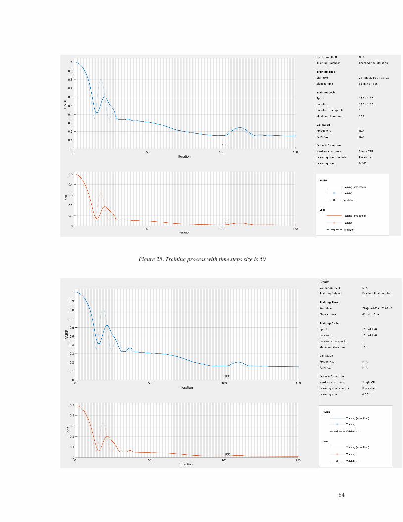
54

Figure 25. Training process with time steps size is 50

55

Figure 26. Training process with time steps size is 300

Figure 27. Training process with time steps size is 600

We can find that while we increase the time steps, our training result is also good enough

for us and the loss of the function is in the range we can accept. This is also proved that

LSTM has an excellent performance in a long time series data sequence. We will test its

performance in the predicted result.

56

7 predict results We have built the different sets of the training process model, but we need to test its

performance in the test data to make sure this model is reliable. Thus we use the test data

to predict the load and compare the accuracy of these models.

7.1 predict And Update State When predicting multiple time steps in the future, we need to use the predicted values and

the updated status values to make predictions on a time-by-step basis, and update the

network status each time. Each prediction uses the previous predicted value as the input to

the function.

Pre-processing the data to standardize it so that the convergence of the entire training

cannot be expected to reach the expected level.

After we preprocess the test data, we have two choices to test our model. The first one is

to update the state use the predict data from the model. Also, the other one has updated the

state with the actual values of time steps between predictions.

7.1.1 predict by the training model First, we test the model performance, which updates the state with the predict data.

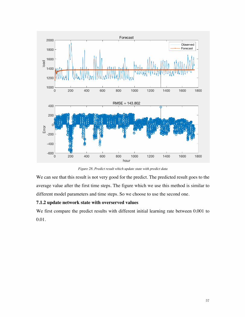
57

Figure 28. Predict result which update state with predict data

We can see that this result is not very good for the predict. The predicted result goes to the

average value after the first time steps. The figure which we use this method is similar to

different model parameters and time steps. So we choose to use the second one.

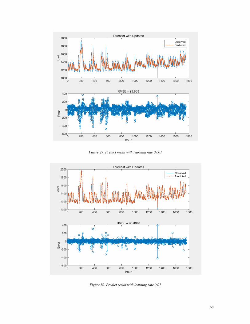
7.1.2 update network state with overserved values

We first compare the predict results with different initial learning rate between 0.001 to

0.01.

58

Figure 29. Predict result with learning rate 0.001

Figure 30. Predict result with learning rate 0.01

59

Figure 31. Predict result with learning rate 0.1

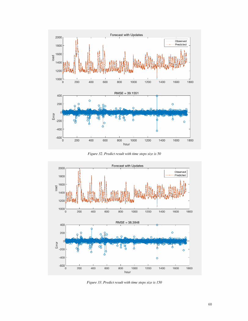
We can find that when the initial learning rate is 0.01, the predicted result is best. Thus

we choose different time steps while setting the initial learning rate 0.01 as a default

value.

60

Figure 32. Predict result with time steps size is 50

Figure 33. Predict result with time steps size is 150

61

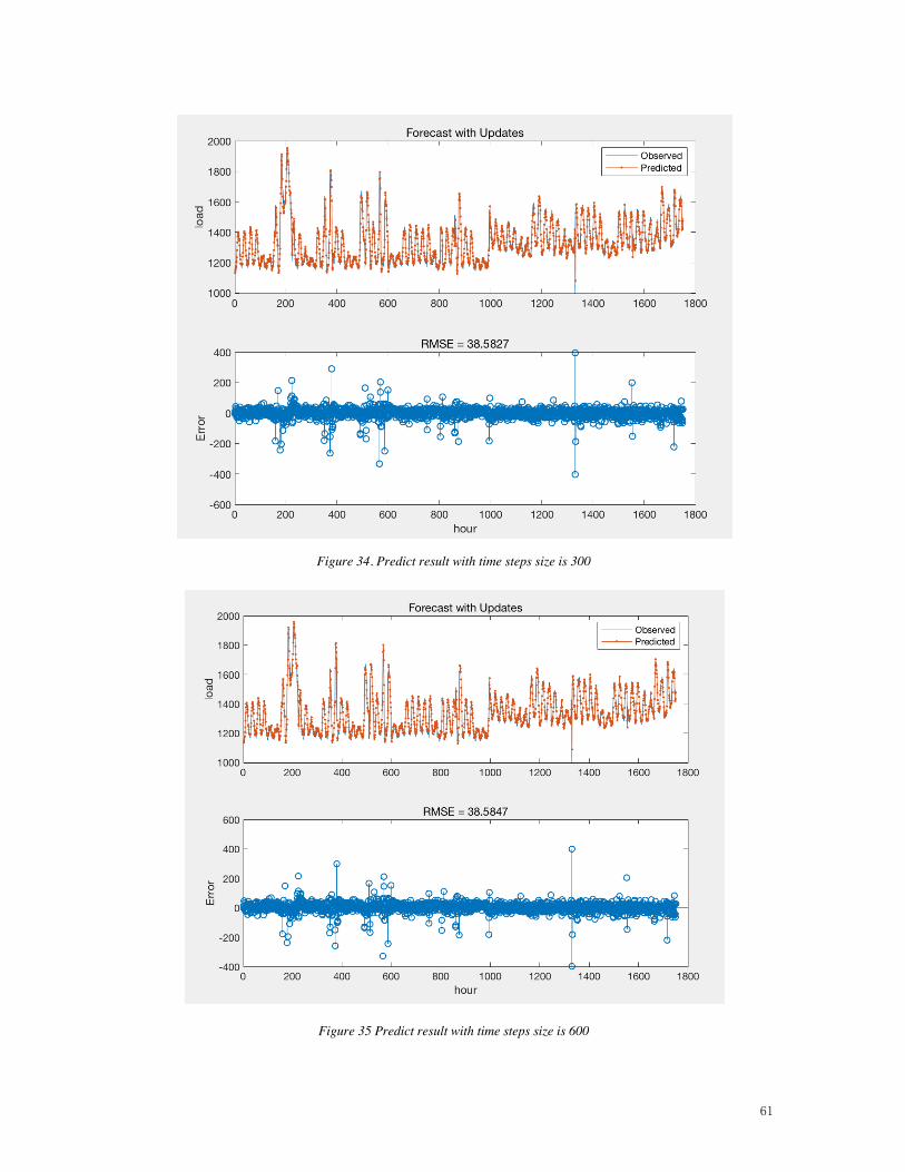
Figure 34. Predict result with time steps size is 300

Figure 35 Predict result with time steps size is 600

62

7.2 Conclusion of the predict result

Table 1 summary of Predict result with initial learning rate

Table 2 summary of Predict result with time steps size

From the figures of the different time-series above. We can find no matter how the time

series of the data changes, the results are always stable, and there are no very sharp

fluctuations. This means LSTM algorithm rare has gradient exploding or vanishing

gradient. Moreover, the predicted results have been in a relatively good range, and there

will be no cliff-like rise or fall changes.

63

8 Conclusion And Future Work In this paper, we proposed a method to optimally tune the parameters of LSTM to forecast

load community power demand. While most of the load data in the power system is always

a long time-series data so it can be used in LSTM without too much preprocess. It has an

outstanding performance to deal with the exploding and vanishing gradient problems in the

long time-series data. We test the different parameters for training the models and try to

find the best one to make load forecasting. After that, we test the model using different

time steps to find the best performance to predict. We can find that the LSTM is a good

algorithm while dealing with long time-series data. It has a very stable performance to

make predictions in a long time steps. Compared with other neural network prediction

methods, its superiority is unquestionable, especially in the case of hour-time in hundreds

of units. That is to say; when we want to predict the load in the next few weeks, LSTM

algorithm practicality is particularly significant. This results dramatically increases the

applicability of LSTM.

From the paper, we know that we can get the result from the LSTM algorithm. However,

we use the load data, which is a single character data. From that data, we can only build a

one-dimensional model to training the data; this has a limited while we deal with the real

data in life. We will try to put more features which can affect the results such as the country,

the date, the season, and many other reasons. If we can put more features, the load

forecasting should be more precise. We also need to make preprocessing data to clean the

data. In this paper, we used all of the data we have. However, we should use preprocessing

the data to select the right data, delete the redundancy data, and noise. These will make our

model more robust.

64

REFERENCES [1] Long short-term memory - Wikipedia. https://en.wikipedia.org/wiki/Long_short-

term_memory

[2] Vossen, J., Feron, B., & Monti, A. (2018). Probabilistic Forecasting of Household

Electrical Load Using Artificial Neural Networks. 2018 IEEE International Conference on

Probabilistic Methods Applied to Power Systems (PMAPS).

doi:10.1109/pmaps.2018.8440559

[3] Mitra, S., & Pal, S. K. (1995). Fuzzy multi-layer perceptron, inferencing and rule

generation. IEEE Transactions on Neural Networks, 6(1), 51-63.

[4] Tsang, W. (n.d.). Kernel methods in supervised and unsupervised learning.

doi:10.14711/thesis-b805964

[5] Ruder, S. (2016). An overview of gradient descent optimization algorithms. arXiv

preprint arXiv:1609.04747.

[6] Johnson, R., & Zhang, T. (2013). Accelerating stochastic gradient descent using

predictive variance reduction. In Advances in neural information processing systems (pp.

315-323).

[7] Neural Networks for Named Entity Recognition. (n.d.). Retrieved from

http://nlp.stanford.edu/~socherr/pa4_ner.pdf

[8] Han, J., & Moraga, C. (1995). The influence of the sigmoid function parameters on the

speed of backpropagation learning. Lecture Notes in Computer Science From Natural to

Artificial Neural Computation,195-201. doi:10.1007/3-540-59497-3_175

[9] Werbos, P. J. (1990). Backpropagation through time: what it does and how to do

it. Proceedings of the IEEE, 78(10), 1550-1560.

[10] Britz, D. (2015). Recurrent neural networks tutorial, part 1–introduction to rnns. 2017-

12-23]. http://www. wildml. com/2015/09/recurrent-neural-networks-tutorial-part-1-

introduction-to-rnns.

[11] Pascanu, R., Mikolov, T., & Bengio, Y. (2013, February). On the difficulty of training

recurrent neural networks. In International conference on machine learning (pp. 1310-

1318).

65

[12] Yao, K., Peng, B., Zhang, Y., Yu, D., Zweig, G., & Shi, Y. (2014, December). Spoken

language understanding using long short-term memory neural networks. In 2014 IEEE

Spoken Language Technology Workshop (SLT) (pp. 189-194). IEEE.

[13] BilstmLayer. (n.d.). Retrieved from

https://www.mathworks.com/help/deeplearning/ug/long-short-term-memory-

networks.html

[14] Qiu, X., Zhang, L., Ren, Y., Suganthan, P. N., & Amaratunga, G. (2014, December).

Ensemble deep learning for regression and time series forecasting. In 2014 IEEE

symposium on computational intelligence in ensemble learning (CIEL) (pp. 1-6). IEEE.

[15] LstmLayer. (n.d.). Retrieved from

https://www.mathworks.com/help/deeplearning/examples/time-series-forecasting-using-

deep-learning.html

[16] SolverName. (n.d.). Retrieved from

https://www.mathworks.com/help/deeplearning/ref/trainingoptions.html