elastic wave propagation in composites and least-squares
TRANSCRIPT

Abstract
WANG, LEI. Elastic Wave Propagation in Composites and Least-squares Damage
Localization Technique. (Under the direction of Dr. Fuh-Gwo Yuan)
The main objective of Structural Health Monitoring (SHM) is to be able to
continuously monitor and assess the status of the integrity of a structure or its components
with a high level of confidence and reliability. In general, the common techniques employed
in SHM for monitoring structures and detecting damages can be divided into two categories:
(1) vibration-based approach and (2) wave-based approach. Since wave-based approach can
provide better local health status information and has higher sensitivity to damages than
vibration-based approach, this thesis focuses on damage localization of plate structure using
wave-based approach by first characterizing elastic waves in composite laminates; then using
a time-frequency signal processing technique to analyze dispersive stress waves; and lastly a
least-squares technique is proposed for damage localization.
Exact solutions of dispersive relations in a composite lamina and composite laminate
are first deduced from three-dimensional (3-D) elasticity theory. The dispersion relations
containing infinite number of symmetric and antisymmetric wave modes are numerically
solved. Then, to make dispersive wave solutions tractable in composites, a higher-order plate
theory is proposed. The dispersion relations of three antisymmetric wave modes and five
symmetric wave modes can be analytically determined. The dispersion curves of phase
velocity and group velocity are obtained from the two theories. From the results of the 3-D
elasticity theory and higher-order plate theory, it can be seen from dispersion curves that the
higher-order plate theory gives a good agreement in comparison with those obtained from 3-
D elasticity theory in the relatively high frequency range; and especially for the lowest

symmetric and antisymmetric modes, dispersion relation curves obtained from the two
theories match very well.
In the Chapter of time-frequency analysis of dispersive waves, a Wavelet Transform
(WT) is directly performed on a transient dispersive wave to extract the time-frequency
information of transient waves. Consequently, the dispersion relations of group velocity and
phase velocity can be mathematically obtained. Experiments are set up to verify the proposed
WT method, in which a lead break is used as a simulated acoustic emission source on the
surface of an aluminum plate. The dispersion curves of both phase and group velocities of the
lowest flexural wave mode obtained from the experiments by using WT show good
agreement with theoretical prediction values.
Having group velocities verified from the experiments, a least-squares method is
proposed to SHM field for iteratively searching damage location based on elastic wave
energy measurements. The method is suitable for achieving automated SHM system since the
proposed method is based on active damage detection technique and deals with the entire
sensor data in the least-squares algorithm without the need of ambiguously measuring the
time-of-flights. The simulated data are obtained from finite difference method in conjunction
with Mindlin plate theory. Simulated examples for damage detection are demonstrated by
using the least-squares method. Moreover, an active SHM system is set up to validate the
feasibility of the least-squares damage localization technique. From the simulated and
experimental results, it is shown that the estimated damage position by least-squares method
gives good agreement with the targeted damage location.

ELASTIC WAVE PROPAGATION IN COMPOISTES AND LEAST-SQUARES DAMAGE LOCALIZATION TECHNIQUE
by
LEI WANG
A thesis submitted to the Graduate Faculty of
North Carolina State University
in partial fulfillment of the
requirements for the Degree of
Master of Science
AEROSPACE ENGINEERING
Raleigh
2004
APPROVED BY:

ii
To my parents
and
Jane

iii
Biography
Lei Wang was born in Dongying, Shandong Province, the People’s Republic of China
on July 1, 1977. Having received his elementary and secondary education in Dongying, he
graduated from the No. 2 Middle School of Shengli Oil Field in 1995. He received his
Bachelor of Science degree in Detecting Technology and Instruments from Nanjing
University of Aeronautics and Astronautics in 1999. Since then he continued his graduate
study in The Aeronautical Science Key Laboratory for Smart Materials and Structures at
Nanjing University of Aeronautics and Astronautics for three years. He started his M.S.
program of Aerospace Engineering at North Carolina State University in the fall of 2002.

iv
Acknowledgements
First of all, I would like to thank Dr. Fuh-Gwo Yuan for suggesting the following
work and serving as my graduate advisor over the past two years. I appreciate very much his
warm guidance and enthusiastic encouragement throughout the work. Especially, his insight
into cross disciplines, prowess of exploring frontier research and perseverance of pursuing
perfection in research impress me greatly and will surely benefit my future academic career.
I would like to thank Drs. Kara Peters, Jeffrey W. Eischen, and Fen Wu for providing
helpful advice in completing this research. I thank Dr. Shaorui Yang for his help and
suggestion in this research. Special thanks go to Dr. Xiao Lin, one of Dr. Yuan’s former
Ph.D. students, who always offers me a warm and in-time assistance whenever I asked for.
This research is supported by the Sensors and Sensor Networks program from the
National Science Foundation (Grant No. CMS-0329878). Dr. S. C. Liu is the program
manager. The financial support is gratefully acknowledged.
Thanks also go to all the members in our research group including Mr. Yun Jin, Mr.
Lei Liu, Ms. Aihua Liang, Mr. Artem Dyakonov, Mr. Saeed Nojovan, Mr. Perry Miller, Mr.
H. Hussein, and Mr. Guoliang Jiang for their care and help. The friendship with them makes
my life in Raleigh brighter and more colorful.
Additionally, my deepest appreciation goes to Mr. Ziyue Liu and his wife, Mr.
Chunwei Wu, Mr. Jibing Li, Mr. Zheng Gao, and Mr. Andrew Bowman who were there
whenever I needed. I would like to express my sincere thanks to all the people from whom I
have received help and advised during my MS study at North Carolina State University.
Finally, I should thank my father, mother and brother. Without their understanding
and encouragement, I could never reach this joyful moment.

v
Table of Contents
List of Tables ............................................................................................................................. viii
List of Figures.............................................................................................................................. ix
Nomenclature and Abbreviations .......................................................................................... xiv
1 Introduction............................................................................................................................... 1
1.1 Structural Health Monitoring .............................................................................................1
1.2 Elastic Waves in Composite Plates ....................................................................................3
1.3 Time-frequency Analysis for Dispersive Waves ..............................................................7
1.4 Least-squares Damage Localization ..................................................................................9
1.5 Summary............................................................................................................................10
2 Elastic Wave Dispersion in Composite Laminates............................................................ 13
2.1 Exact Solutions for Wave in a Composite Plate .............................................................14
2.1.1 Waves in a composite lamina........................................................................................14
2.1.2 Waves in a composite laminate.....................................................................................21
2.2 Transient Waves in Composites Based on a Higher-order Plate Theory ......................29
2.2.1 Constitutive relations....................................................................................................30
2.2.2 Determination of iκ .....................................................................................................38
2.3 Phase and Group Velocity ................................................................................................39
2.3.1 Concepts of phase and group velocity ...........................................................................39
2.3.2 Determination of phase velocity ...................................................................................41
2.3.3 Determination of group velocity ...................................................................................41
2.4 Numerical Examples.........................................................................................................44
3 Wavelet Analysis for Dispersive Waves in Plates.............................................................. 58
3.1 Continuous Wavelet Transform .......................................................................................58

vi
3.2 Gabor Wavelet Function...................................................................................................60
3.3 Implementation of Gabor Wavelet Transform ................................................................64
3.3.1 Discretization of CWT..................................................................................................64
33..2 Time-scale to physical time-frequency..........................................................................64
3.3.3 Add Gabor function to wavelet toolbox of Matlab®.......................................................66
3.4 Time-frequency Analysis of Dispersive Waves..............................................................67
3.4.1 Time-frequency analysis by wavelet transform .............................................................67
3.4.2 Determination of group and phase velocities.................................................................69
3.5 Theory on Dispersion of Flexural Waves........................................................................71
3.6 Experimental Study...........................................................................................................74
3.6.1 Experimental setup.......................................................................................................74
3.6..2 Determination of group and phase velocities ................................................................75
3.6.3 Results and discussion..................................................................................................78
4 Least-squares Damage Localization Using Elastic Wave Energy Measurements ....... 81
4.1 An Elastic Wave Energy Decay Model ...........................................................................82
4.2 Least-squares Damage Localization Method ..................................................................85
4.3 Simulations and Experiments ...........................................................................................88
4.3.1 Simulation examples ....................................................................................................88
4.3.2 Experimental study.......................................................................................................90
5 Discussion and Conclusions ................................................................................................ 102
5.1 Conclusions .................................................................................................................... 102
5.2 Future Studies................................................................................................................. 103
6 References .............................................................................................................................. 105
Appendix ................................................................................................................................... 114

vii
A.1 Elastic Coefficients ijC Calculated from ijC ′ by Coordinate Transformations......... 114
A.2 Elastic Coefficients ijC ′ in the Principal Material Coordinate System ...................... 116
A.3 Matlab Script Files: gabor.m and gabinfo.m ............................................................... 117
A.4 Bandwidth of a Signal................................................................................................... 119
A.4.1 3-dB bandwidth ........................................................................................................ 119
A.4.2 Standard deviation bandwidth................................................................................... 121
A.5 Derivation of Eq. (3.4-10) from Eq. (3.4-9) ................................................................ 122
A.6 Source Localization using Triangulation Method....................................................... 125
A.6.1 Isotropic plates ......................................................................................................... 125
A.6.2 Summary of the triangulation method (Tobias, 1976)................................................ 128
A.6.3 Anisotropic plates..................................................................................................... 129
A.6.4 Summary of the triangulation method (Jeong and Jang, 2000)................................... 133
A.6.5 Numerical Simulation............................................................................................... 134

viii
List of Tables
Table 2.1 Material properties of IM7/5250-4 lamina type (fiber volume fraction, Vf =
64%)…………………………………………………………………………..49
Table 3.1 Material properties and geometry of Al 6061 plate …………………..……..74

ix
List of Figures
Figure 2.1 Geometry of an N-layered laminate..………………………………………...23
Figure 2.2 Force and moment resultants on a laminated composite plate..…...………...30
Figure 2.3 Illustration of group velocity………...……………………………………....41
Figure 2.4 Phase velocity distribution of symmetric waves in IM7/5250-4 lamina with
dimensionless frequency 25.0=Lchf ….…………………………………..50
Figure 2.5 Phase velocity distribution of antisymmetric waves in IM7/5250-4 lamina
with dimensionless frequency 15.0=Lchf ………………………………..50
Figure 2.6 Phase velocity distribution of symmetric waves in [90/60/90/-60/0]s
IM7/5250-4 laminate with dimensionless frequency 25.0=Lchf ………...51
Figure 2.7 Phase velocity distribution of antisymmetric waves in [90/60/90/-60/0]s
IM7/5250-4 laminate with dimensionless frequency 15.0=Lchf ………...51
Figure 2.8 Comparison of phase velocity dispersions of symmetric waves from higher-
order plate theory and 3-D elasticity theory with wave propagating along 45°
in IM7/5250-4 lamina………………………………...............................…...52
Figure 2.9 Comparison of group velocity dispersions of symmetric waves from higher-
order plate theory and 3-D elasticity theory with wave propagating along 45°
in IM7/5250-4 lamina………………………………………………………..52
Figure 2.10 Comparison of skew angles of symmetric waves from higher-order plate
theory and 3-D elasticity theory with wave propagating along 45° in
IM7/5250-4 lamina…………………………...………………..………...…..53
Figure 2.11 Comparison of phase velocity dispersions of antisymmetric waves from
higher-order plate theory and 3-D elasticity theory with wave propagating
along 45° in IM7/5250-4 lamina………………………………...............…...53

x
Figure 2.12 Comparison of group velocity dispersions of antisymmetric waves from
higher-order plate theory and 3-D elasticity theory with wave propagating
along 45° in IM7/5250-4 lamina……………………………………………..54
Figure 2.13 Comparison of skew angles of antisymmetric waves from higher-order plate
theory and 3-D elasticity theory with wave propagating along 45° in
IM7/5250-4 lamina…………………………...………………..………...…..54
Figure 2.14 Comparison of phase velocity dispersions of symmetric waves from higher-
order plate theory and 3-D elasticity theory with wave propagating along 45°
in [90/60/90/-60/0]s IM7/5250-4 laminate…………………………….……..55
Figure 2.15 Comparison of group velocity dispersions of symmetric waves from higher-
order plate theory and 3-D elasticity theory with wave propagating along 45°
in [90/60/90/-60/0]s IM7/5250-4 laminate…………………………………...55
Figure 2.16 Comparison of skew angle of symmetric waves from higher-order plate theory
and 3-D elasticity theory with wave propagating along 45° in [90/60/90/-
60/0]s IM7/5250-4 laminate……………………………………………….…56
Figure 2.17 Comparison of phase velocity dispersions of antisymmetric waves from
higher-order plate theory and 3-D elasticity theory with wave propagating
along 45° in [90/60/90/-60/0]s IM7/5250-4 laminate………………………..56
Figure 2.18 Comparison of group velocity dispersions of antisymmetric waves from
higher-order plate theory and 3-D elasticity theory with wave propagating
along 45° in [90/60/90/-60/0]s IM7/5250-4 laminate………………………..57
Figure 2.19 Comparison of skew angle of antisymmetric waves from higher-order plate
theory and 3-D elasticity theory with wave propagating along 45° in
[90/60/90/-60/0]s IM7/5250-4 laminate……………………………………..57
Figure 3.1 (a) The Gabor function; (b) its Fourier transform for 2ln2πγ =
and πω 20 = …………………………………..……….……………………..61

xi
Figure 3.2 (a) The real parts of different Gabor functions when 7,356.5,4=γ ; (b) their
Fourier transforms…………………...............…………….………………....63
Figure 3.3 Experimental setup for the measurement of plate wave velocities……..…....75
Figure 3.4 Waveform collected at sensor S1……..……….……………...……………...77
Figure 3.5 3-D view of the WT at sensor S1………………...……...………...…………77
Figure 3.6 Contour plot of the WT at sensor S1……………..……..................................77
Figure 3.7 Waveform collected at sensor S2………………………..…….………...…...77
Figure 3.8 3-D view of the WT at sensor S2…..………….…………..………...……….77
Figure 3.9 Contour plot of the WT at sensor S2……….……...……..…………………..77
Figure 3.10 The magnitude of WT coefficients of sensor S1 at scale 20 (250kHz)..……..79
Figure 3.11 The phase angle of WT coefficients of sensor S1 at scale 20 (250kHz)……..80
Figure 3.12 The unwrapped phase angle of WT coefficients of sensor S1 at scale 20
(250kHz)…………………..………………………..………...…………..….80
Figure 3.13 The magnitude of WT coefficients of sensor S2 at scale 20 (250kHz)...…….79
Figure 3.14 The phase angle of WT coefficients of sensor S2 at scale 20 (250kHz)……..80
Figure 3.15 The unwrapped phase angle of WT coefficients of sensor S2 at scale 20
(250kHz)……………………………………………………………...……...80
Figure 3.16 Measured and theoretical group/phase velocities of flexural dispersive
waves……………………………………………………….…………..…….80
Figure 4.1 Dispersion curves of flexural waves from Lamb wave theory and Mindlin
plate theory…………………………………………………………………...93
Figure 4.2 Scheme of sensor/actuator deployment and unknown damage..…….………93

xii
Figure 4.3 Simulated reflected wave packs from the damage using finite difference
method……………………………………………………………………….94
Figure 4.4 Simulated reflected wave packs with the zero-mean additive Gaussian
noise………………………………………………………………………….94
Figure 4.5 Single damage localization using three sensors…….…….…….……..…......96
Figure 4.6 Single damage localization using four sensors ……………….........………..97
Figure 4.7 Experimental setup for damage localization………………………....………98
Figure 4.8 The excitation waveform, the response wave signals before and after damage,
and the reflected waves at sensor 3.……………………………………....….98
Figure 4.9 The reflected wave signal received by each sensor …….…………….…..…99
Figure 4.10 Tree decomposition algorithm of DWT and bandwidth of each level .……...99
Figure 4.11 The original signal at sensor 3, its decomposed signals by DWT and
extraction of the first reflection at level 3………..………………………....100
Figure 4.12 The reconstructed signal at sensor 3 by using DWT and extraction of the first
reflected wave signal ………………………………………………...…..…100
Figure 4.13 The reflected wave packs directly from the damage received from each sensor
after DWT.………………………………………………………………….101
Figure 4.14 Experimental result of damage localization by least-squares method …..…101
Figure A.1 An arbitrarily orientated lamina with global and principal material coordinate
systems…………………………………………………………………….. 114
Figure A.2 Illustration of 3-dB bandwidth of Gabor function 1.3863)(ˆ =∆ ωψ g ...……120
Figure A.2 Illustration of standard deviation bandwidth of Gabor function
1.7015)(ˆ =∆ ωψ g …………..………………………………………………122

xiii
Figure A.4 Source location by triangulation method for an isotropic plate………….…126
Figure A.5 Source location analysis for an anisotropic plate………………………...…130
Figure A.6 Numerical simulation of source location in anisotropic plate with source at (6,
4) m denoted by “x”………………………………………………………...135
Figure A.7 Numerical simulation of source location in isotropic plate with source at (6, 4)
m denoted by “x”…………………………………………………………...135
Figure A.8 Numerical simulation of source location in anisotropic plate with source at
(10, 10) m denoted by “x”…………………………………………………..136
Figure A.9 Numerical simulation of source location in isotropic plate with source at (10,
10) m denoted by “x” …………………………………………………........136

xiv
Nomenclature and Abbreviations
Greek Symbols
α Reflection factor at the damage
zyx εεε , , Normal strain components
φ Direction of wave propagation or direction of wavenumber
xφ , yφ Higher-order terms in the expression of displacement fields
ϕ Skew angle of group velocity
ijΓ Elements of the determinant defined in Eq. (2.1-9)
γ Sensor gain factor at a sensor
xyxzyz γγγ , , Engineering shear strain components
κ Shear correction factor
ν Poisson’s ratio
θ Phase angle
ϑ Fiber orientation of a lamina
ρ Damage position vector
ρ Mass density
Σ Stress components along z direction on outer surfaces of a composite laminate
σ Contracted notation of stress components in the global coordinates
σ′ Contracted notation of stress components in the principal material coordinates
zyx σσσ , , Normal stress components
ς Updated step size in least-squares algorithm

xv
τ Time delay from the actuator to the damage
xyxzyz τττ , , Shear stress components
υ Zero-mean additive white Gaussian noise
ω Angular frequency
ψ Mother wavelet or base wavelet function
xψ , yψ Rotations of section x = constant and y = constant, respectively
Roman Symbols
A, B, C Displacement constants defined in Eq. (2.1-8)
a Scale parameter in Wavelet Transform
0a Normalized reflected waveform from damage
b Translation parameter in Wavelet Transform
Cij Components of stiffness matrix in the global coordinates
ijC′ Components of stiffness matrix in the principal material coordinates
ψC Admissible condition
cg Group velocity
Lc Longitudinal wave velocity in the direction of fiber orientation ρ11CcL =
cp Phase velocity
D Matrix variable defined in Eq. (2.1-32)
D Plate bending stiffness, )1(12 2
3
v
EhD
−=
E Young’s modulus
E Mathematical expectation operator

xvi
f Frequency
fs Sampling rate
G Local transfer matrix defined in Eq. (2.1-24)
G Shear modulus
g Square of sensor gain factor at a sensor
Hij Variables defined in Eq. (2.1-16)
h Thickness of the plate
I Moment of inertia
J Least-squares error function
k Wavenumber vector
k Magnitude of wavenumber
L Variables defined in Eq. (2.2-11)
l Direction cosines of wave propagation
M Moment resultant / unit length
N Axial force / unit length
P Vector variable defined in Eq. (2.1-25)
p Solutions of Eq. (2.1-11)
Q Transformation matrix
Q Shear force / unit length
q Five-peak excitation signal
R, S Variables defined in Eq. (2.1-13), higher-order resultants
r Cartesian coordinates of a sensor
s Modeled received signal without additive noise at a sensor

xvii
Re Real part of a complex variable
T Matrix variable defined in Eq. (2.1-26)
t Time variable
u, v, w Displacement components in the direction of x, y and z, respectively
U, V, W Displacement components which are function of z and defined in Eq. (2.1-5)
U ′ , V ′ , W ′ Derivatives of U, V, W with respect to z, respectively
Vf Fiber volume fraction
x, y, z Cartesian coordinates
x Modeled received signal with additive noise at a sensor
y Measured wave energy at a sensor
Z Modeled wave energy at a sensor
Subscripts
0 Variables on the middle plane of the plate in Section 2.2
c Denotes central frequency
m Sensor number
n Layer number of composite laminates
g Denotes Gabor function
x, y, z Components along the direction of Cartesian coordinates
Superscripts
i Epoch of the least-squares algorithm
T Transpose operator
+, - Displacements or stress variables on the upper and lower surfaces of layer n

xviii
Caps
Stress components divided by ik
^ Variables in frequency domain
~ Nondimensional variables
- Complex conjugate
· Derivative with respect to time
Abbreviations
3-D Three-dimensional
CEV Crew Exploration Vehicle
CPT Classical Plate Theory
CWT Continuous Wavelet Transform
DOA Direction of Arrival
DWT Discrete Wavelet Transform
NDE Non-destructive Evaluation
PZT Lead Zirconate Titanate
SDPT Shear Deformation Plate Theory
SH Shear Horizontal wave
SHM Structural Health Monitoring
SNR Signal to Noise Ratio
STFT Short Time Fourier Transform
TDOA Time Difference of Arrival
WT Wavelet Transform
WVD Wigner-Ville Distribution
)

1
1 Introduction
1.1 Structural Health Monitoring
The integrity of critical structures such as aircrafts, civil infrastructures, mechanical
systems, etc., needs to be monitored in-situ and real-time to detect damage at an early stage.
Traditional Non-destructive Evaluation (NDE) techniques can not be directly applied to
monitor the health status of structures since these techniques usually rely on in-laboratory
testing and require bulky instruments (Thomas, 1995). Especially for aerospace vehicles, the
health monitoring system requires to perform on in-service structures with minimum manual
interference. Therefore, integrated monitoring components such as sensors, either surface-
mounted or embedded in the structures are compulsory in these circumstances (Boller, 1997).
A structural health monitoring (SHM) system with built-in sensors has attracted much
attention in the past decade (Chang, 1999; Doebling et al., 1996; Hall, 1999; Housner et al.,
1997; and Sohn et al., 2004). Besides sensors, actuators exciting diagnostic signals can also
be surface-mounted on or embedded in the structures to build an active SHM system. A
major advantage of the active SHM system over a passive one (without built-in actuators) is
that the active SHM is subjected to a prescribed actuation and thus increases the accuracy
and reliability of assessing the structural status from the collected sensor data.
For real applications of SHM in aerospace, Boeing’s new 7E7 aircraft will have a
full-time built-in SHM system with sensors embedded in the structure to evaluate the state of
structural health (Butterworth-Hayes, 2003). According to NASA’s requirements on the new
Crew Exploration Vehicle (CEV), Lockheed Martin’s Atlas V and Boeing’s Delta IV
satellite launchers will soon have integrated health monitoring system to assess the overall

2
health of the vehicle continually during the ascent to spot a problem before it becomes
catastrophic (Lannotta, 2004).
Detecting the location and identifying the dimension and form of damages are the
primary goals of a SHM system. Generally, the common techniques of damage identification
employed in SHM can be roughly divided into two categories: (1) vibration-based approach
and (2) wave-based approach. Vibration-based technique can be considered as a global
damage detection method, where the performance of the entire structure or system is
monitored and verified. Wave-based technique can be regarded as a local damage detection
method and only the certain key elements of the total system are interested in monitoring.
Numerous investigators have applied vibration-based methods to detect damage
existence and attempt to localize damages mainly in civil structures such as bridges,
highways, and buildings. However, there are several essential disadvantages limiting the
extensive application of vibration-based damage detection methods. First, vibration-based
approaches have low sensitivity to damage. The basic premise of most vibration-based
damage detection methods is that damage will alter the stiffness, flexibility, mode shape, etc.,
which in turn alter the measured dynamic response of the structure such as resonant
frequencies and mode shapes. However the damage is typically a local phenomenon, at least
in the beginning stage, and may not significantly influence the global response of a structure
that is normally measured from the vibration test. Second, a limited number of lower modes
and truncated mode shapes that can be reliably determined can lead to systematic error. In
vibration-based methods, the response measurement can be expressed in terms of a
superposition of all mode shapes, but only a limited number of modes may be accessible in
practice because of limited number of sensor measurements and loss of fidelity in higher

3
modes. Third, environmental and operational variations, such as varying temperature,
moisture, loading conditions, and boundary conditions affecting the dynamic response of the
structures can not be overlooked either (Farrar et al., 1994). These effects impair reliability
of damage detection.
Wave-based damage detection however excites transient waves propagating in
structures by actuators ( or active sensors), since the waves will be reactive to damages such
as reflection, scattering or dissipation, the health status of structures will be estimated by
analyzing the response waves received by either surface-bonded or embedded sensors.
Compared with vibration-based method, wave-based method can effectively obtain the local
information of structures and can accommodate variations of boundary conditions and
temperatures (Sohn et al., 2004). Many investigators have applied transient wave-based
damage detection techniques to localizing damages and even quantifying the dimension of
damage either in isotropic (e.g., Gaul and Hurlebaus, 1997; Hurlebaus, 2001; Lin and Yuan,
2001b; Quek et al., 2001; and Giurgiutiu et al, 2002), or in anisotropic materials (e.g.,
Cawley, 1994; Guo and Cawley, 1994; Tan et al., 1995; Birt, 1998; Jeong and Jang, 2000;
Wang and Yuan, 2003; Sohn et al., 2004; and Ihn and Chang, 2004).
1.2 Elastic Waves in Composite Plates
The propagation of waves in an infinite elastic plate has been studied since 1889
dispersive waves based on the theory of elasticity in plane strain. For plane waves traveling
in a free isotropic plate case, the waves are a combination of longitudinal and vertically
polarized shear bulk waves propagating in a direction parallel to the plate. These two types of
waves are coupled by the reflections in the plate. The resulting guided waves traveling along
the plate axis in an isotropic material are called Lamb waves, which may have symmetric and

4
antisymmetric modes. The theory of Lamb waves has been fully documented in a number of
textbooks (Viktorov, 1967 and Graff, 1991) and it has been widely applied in NDE
(Krautkramer and Krautkramer, 1990; Blitz and Simpson, 1996; Hurbelaus et al., 2001; and
Wilcox et al., 2001). In recent years, several investigators have also applied Lamb waves for
SHM of isotropic materials. Lin and Yuan (2001a) analytically modeled Lamb wave signal
generated and collected by piezoelectric (PZT) actuator/sensor. This model first combined
the analytical solution of Mindlin plate theory and piezoelectric effect of the actuator/sensor,
thus the voltage output of a sensor can be obtained directly from voltage input of the
actuator. Giurgiutiu et al. (2002) investigated a Lamb waves based SHM of both aluminum
beam and plate with integrated PZT sensors and actuators.
The increasing use of advanced composites in structural components, such as
aerospace structures, marine vehicles, automotive parts, and many other applications has led
to extensive research activities in the field of composite materials. The most widely used
composite structures are laminates consisting of many fiber-reinforced laminae that are
bonded together to achieve more desirable structural properties and better performance than
conventional materials. To understand the dynamic response for use in damage detection, the
theory of elastic waves in composite laminates is desirable to be developed. Due to
anisotropic and multilayered properties of laminates, however, the exact analytical treatment
of waves in composites is much more complicated and consumes more computational cost
than that of waves in an isotropic plate.
Some of the difficulties in the treatment of wave propagation in anisotropic plates can
be illustrated by considering slowness wave surface methods for infinite media (Synge, 1957;
Fedorov, 1968; and Musgrave, 1970). Perhaps the most significant consequence of elastic

5
anisotropy is the loss of pure wave modes for general propagation directions. This fact also
implies that the direction of group velocity (i.e., energy flow) does not generally coincide
with the wave vector or wave front normal (Fedorov, 1968). In addition, the distinction
between wave mode types in generally anisotropic plates is somewhat artificial, since the
equations for classical Lamb and shear horizontal (SH) modes and symmetric and
antisymmetric modes generally are coupled. Therefore, we will refer to these modes as
elastic waves in plates (Nayfeh and Chimenti, 1989).
Tang et al. (1989) investigated the flexural wave motion in symmetric cross-ply and
quasi-isotropic laminates by both elasticity theory and first-order plate theory, and then
compared the analytical results with the experimental results. Nayfeh and Chimenti (1989)
gave dispersion relation curves of elastic wave in general one-layered anisotropic media, i.e.,
composite lamina. Nayfeh (1991) developed a transfer matrix technique to obtain the
dispersion relation curves of elastic waves propagating in multilayered anisotropic media,
i.e., composite laminate. However, Nayfeh’s formulation (1989, 1991) was limited to a given
plane of incidence from a line load parallel to the y-axis such that the problem reduces to
generalized plane deformation where all the three displacement components are functions of
x and z. Yuan and Hsieh (1998) obtained the exact solutions of elastic waves in composite
cylindrical shell based on both 3-D anisotropic elasticity theory and compared them with
Flügge shell theory. However, these studies only obtained the dispersion relations of phase
velocity, but not extended to group velocity. Besides the dispersion relations, several
researchers also have studied the transient elastic waves in composite laminates (Liu et al.,
1991 and Mal and Lih, 1992).

6
Approximate plate theories have been extremely useful in providing analytical
solutions to a variety of problems involving static and dynamic response of laminated plates
of finite dimensions under external loads. Furthermore, for computing the dispersion
relations of elastic waves in composites, approximate plate theories can offer much higher
computational efficiency than 3-D elasticity theory since approximate plate theories avoid
solving time-consuming transcendental equations. This feature of approximate plate theories
is very useful to achieve a real-time SHM system in practice. The laminated plate theories are
direct extensions of those developed earlier for homogeneous isotropic and orthotropic
plates, where use is made of displacement fields which do not account for interface
continuity explicitly between the lamina. In the simplest approximation, namely, the
Classical Plate theory (CPT) based on the Kirchhoff hypotheses have been developed by
Reissner and Stavsky (1961), Dong, Pister and Taylor (1962), and summarized by Ashton
and Whitney (1970). These works were based on a linear displacement across the entire
laminate with shear deformation neglected. An improved Mindlin-type (Mindlin, 1960) first-
order transverse shear deformation plate theory (SDPT) was developed by Whitney and
Pagano (1970) for composite laminates. In this theory, linear displacements were assumed
across the entire laminate thickness; however, transverse shear deformation was not
neglected. Higher-order shear deformation theories have been proposed by other researchers
(Lo et al., 1977 and Reddy, 1984).
Since the symmetric wave motion is a promising mode for long range inspection and
has proposed several methods by which damage can be detected in composite laminates,
especially for delamination damage (Cawley, 1994; Guo and Cawley, 1992; and Birt, 1998),
the approximate plate theory for symmetric waves in laminates are needed to be developed

7
for SHM. Kulkarni and Pagano (1972) presented the both 3-D elasticity theory and an
approximate theory for vibration of elastic laminates. Due to a first-order SDPT, the
dispersion of the first symmetric mode was not predicted by this theory. Whitney and Sun
(1973) extended the above theory to a higher-order theory including the first symmetric
thickness shear and thickness stretch modes by considering higher-order terms in the
displacement expansion about the mid-plane of the laminate in a manner similar to that of
Mindlin and Medick (1959) for homogeneous isotropic plates. These theories have been
focused on the vibration problem of composites. The existing higher-order plate theory still
needs to be extended to analyze elastic waves propagating along arbitrary direction in
composites.
1.3 Time-frequency Analysis for Dispersive Waves
One of the main objectives of SHM is to extract certain physical parameters from
measured data in structures and then to use them to quantify the health status of structures.
Since the ultrasonic waves generated from initiation of the damage and/or reflected from the
damage carry the information about the damage, the characterization of waves such as its
dispersion curves needs to be further understood. In general, the phase and group velocities
of dispersive waves propagating in plate-like solids are related to the geometry and material
properties. Thus, evaluating the dispersion of phase and group velocities with sensible
physical information is of practical importance in SHM.
In SHM, signal processing plays an essential role to physically interpret the collected
data records from sensors, extract health status information of structures, and even improve
the decision on damage detection. Generally the collected signals are non-stationary time
series in nature. Traditional Fourier analysis is obviously unsuitable for processing these time

8
series since it is mainly a stationary time series based processing technique and is unable to
simultaneously provide both time and frequency information. In the past, the Fourier
transform has been extensively used for the analysis of dispersive wave signals (Sachse and
Pao, 1978; Wu and Chen, 1996). In recent years, some advanced techniques based on the
time-frequency analysis were applied to study waves in solids, such as Short-Time Fourier
Transform (STFT) (Hodges, Power and Woodhouse, 1985) and Wigner-Ville Distribution
(WVD) (Latif et al., 1999). However, because of the constant window structure employed in
STFT, it is not capable of providing sufficient resolution over a wide spectral range.
Furthermore, since WVD is defined as the Fourier transform of the central covariance
function of a given signal and has quadratic structure, it inevitably generates interference
terms that incur spurious information to the results of WVD.
Compared with these techniques, Wavelet Transform (WT) appears to be a very
attractive signal processing technique for non-stationary signals and has been proved to be a
more versatile and effective tool for studying dispersive waves. One of the earliest
introductory works on dispersive waves using WT is by Önsay and Haddow (1995). They
selected a complex Morlet wavelet as a mother wavelet function but did not examine the
dispersion relations of phase and group velocities. Kishimoto et al. (1995) applied a Gabor
wavelet to time-frequency analysis of flexural waves and obtained the dispersion relations of
group velocity from numerically simulation data of an Euler beam. In addition, Quek et al.
(2001) investigated several key practical issues on the application of Gabor wavelet to
dispersive waves such as sampling rate, choice and resolution of wavelet scales.
Furthermore, by knowing the dispersion relation, a couple of practical NDE applications
were developed from WT. For example, Gaul and Hurlebaus (1997) applied the Gabor WT to

9
an impact load location on aluminum plate and Sohn et al. (2004) located the multiple
delamination damages in a quasi-isotropic laminate by using WT; Jeong and Jang (2000) and
Jeong (2001) obtained the group velocity of the lowest mode of flexural waves and detect a
source location of an acoustic emission event in a composite laminates by using Gabor WT.
Besides the Gabor WT in dispersion research, another common used WT is harmonic WT,
which is one of orthogonal wavelets and has compact supports in the frequency domain,
developed by Newland (1993, 1997, 1998, and 1999). However, in the previous research
either by Kishimoto et al. (1995), Jeong and Jang (2000), or Jeong (2001), the time-
frequency analysis of dispersive waves to obtain the group velocity was not mathematically
rigorous, where WT were performed on a much simpler case that two harmonic waves with
close frequency propagate together. In addition, those studies can merely obtain the
dispersive group velocity determined from time-frequency map of WT, not the phase
velocity.
1.4 Least-squares Damage Localization
Mathematically, locating damage is an inverse problem. The estimated damage
location may be calculated from collected signals such that the error function can reach its
minimum. The proposed least-squares damage localization technique utilizes the real-valued
signals reflected from a single damage and iteratively searches damage position until a error
function reaches its minimum value.
For conventional damage detection techniques, the wave velocity and time-of-flight
or arrival time of damage reflected waves need to be measured, and then with specific
algorithms the damage position can be detected (Kehlenbach and Hanselka, 2003; Jeong,
2001; Wang et al; and Ihn and Chang, 2004). Since the excitation is narrow-band and has a

10
finite envelope in time domain, the ambiguity of evaluating of time-of-flight, which is based
on detecting the peak of envelope of damage reflected waves, is not negligible.
Existing acoustic source localization methods make use of three common types of
physical measurements: time difference of arrival (TDOA), direction of arrival (DOA), and
source signal strength or energy. DOA can be estimated by exploiting the phase difference
measured at received sensors (Haykin, 1985; Taff, 1997; and Kaplan et al., 2001) and is
applicable when the acoustic source emits a coherent narrow band signal. TDOA is suitable
for broadband acoustic source localization and has been extensively investigated (Yao et al.,
1998 and Reed et al., 1999). It requires accurate measurements of the relative time delay
between sensors. It is known that the intensity or equivalently the energy of acoustic signal
attenuates as a function of distance from the source. Using this property, recently, an energy-
based acoustic source localization method has been reported (Sheng and Hu, 2003). Since the
TDOA needs a sensor array and a large number of sensors and DOA has to detect the arrival
time, these two methods are not suitable for extending then in SHM. Thus, the third approach
based on wave energy measurement is more suitable and feasible in a practical SHM system.
1.5 Summary
The main content of this study is covered in Chapter 2 through Chapter 5. In Chapter
2, the exact solutions of elastic waves in one-layered anisotropic plate based on 3-D elasticity
theory are established, and then are extended to a multi-layered anisotropic plate (composite
laminate) with an arbitrary stacking sequence. The dispersion relations of both infinite
symmetric and antisymmetric wave modes can be numerically obtained. A higher-order plate
theory for waves in laminates is also developed based on a method developed by Whitney
and Sun (1973). Three modes of antisymmetric wave modes and five modes of symmetric

11
wave modes are derived from the proposed approximate plate theory. Besides the dispersion
curves of phase velocity, the dispersion curves of group velocity for elastic waves in
IM7/5250-4 graphite/epoxy composite laminate are computed. For each numerical example,
the dispersion relations calculated from 3-D elasticity theory are compared with the results
obtained from the higher-order plate theory.
In Chapter 3, WT is used to analyze the dispersion relations of elastic waves in a
plate. WT is directly performed on a dispersive wave to extract the time-frequency
information. Consequently, the dispersion relations of not only group velocity but also phase
velocity can be mathematically obtained. Experiments are performed by using a lead break as
the simulated acoustic emission source on the surface of an aluminum plate. The dispersion
curves of both phase and group velocities obtained from the experiments by using WT show
good agreement with theoretical prediction values.
In Chapter 4, a least-squares method is first introduced to iteratively search damage
location in plates by using energy measurement of elastic waves. An elastic wave energy
decay model for wave propagating in plates is first derived. Then the least-squares method is
applied to iteratively searching damage localization based on elastic wave energy
measurements. The proposed method possesses several advantages over other triangulation
methods. First the method can be used in the active damage detection which is suitable for
the applications of SHM. Second the signals collected by sensors are used in the model
without measuring the time-of-flight or arrival time which oftentimes is ambiguous to be
measured. Lastly, environmental noise can be readily taken into account in the model. An
active SHM system is set up to validate the feasibility of the least-squares damage
localization method. From the simulated and experimental results on an aluminum plate, it is

12
shown that the estimated damage position by least-squares method provides good agreement
with the targeted damage location.
Chapter 5 summarizes the contributions and conclusions of this study and also
proposes some perspective topics for the future research.

13
2 Elastic Wave Dispersion in Composite Laminates
In describing elastic wave propagation in symmetric laminates, there exist two types
of uncoupled wave motion: symmetric (extensional and/or shear horizontal) waves and
antisymmetric (flexural and/or shear horizontal) waves. Under general excitation in a plate,
these types of waves may usually co-exist.
In this Chapter, dispersion curves in laminated composite plates are modeled by both
3-D elasticity theory and a higher-order plate theory. The advantage of using 3-D elasticity
theory is obvious in that the “exact” solutions hold for all frequency ranges. However, the
exact solutions consist of infinite wave modes, symmetric or antisymmetric motions. The
mode conversions that occur when the wave mode interacts with inhomogeneity add
additional complexities. Although 3-D elasticity solutions can provide an exact modeling
capability, computational cost is too high to achieve real-time processing for SHM, not to
mention the transcendental equations inevitably need to be numerically solved for dispersion
curves. Thus, a higher-order plate theory is examined to obtain approximate solutions of
waves in composites. Three modes of antisymmetric wave and five modes of symmetric
wave can be obtained from the higher-order plate theory.
Dispersion relations of symmetric and antisymmetric waves in both composite lamina
and laminates are analyzed. The relations are illustrated in IM7/5250-4 graphite/epoxy
lamina and laminates. The validity of the approximate dispersion relations based on the
higher-order plate theory is made in comparison with those from 3-D elasticity theory. From
these numerical results, it may be observed that the higher-order plate theory give a very
good agreement in the relatively high frequency range.

14
2.1 Exact Solutions for Wave in a Composite Plate
In this section, a rectangular Cartesian coordinate system x, y and z axis is used with z
axis normal to the mid-plane of plate spanned by x and y axis. A wave propagates in a
composite plate in an arbitrary direction that can be described by an angle φ with respect to x
axis. First, 3-D elasticity theory is used to model the waves in a composite lamina to obtain
closed-form dispersion relations. Then, imposing continuity of displacements and tractions
along the interfaces with traction-free surface conditions, the dispersion of waves in
composite laminates may be computed.
Nayfeh and Chimenti (1989) gave dispersion curves of elastic wave in general one-
layered anisotropic media, i.e., composite lamina. Nayfeh (1991) developed a transfer matrix
technique to obtain the dispersion relation curves of elastic wave propagating in multilayered
anisotropic media, i.e., composite laminate. However, Nayfeh’s formulation (1989, 1991)
was limited to a given plane of incidence from a line load parallel to the y-axis such that the
problem reduces to generalized plane deformation where all the three displacement
components are functions of x and z.
2.1.1 Waves in a composite lamina
Consider a composite lamina with surfaces at 2hz ±= , the stress-strain relations for
a monoclinic material with respect to z axis are given by:

15
=
xy
xz
yz
z
y
x
xy
xz
yz
z
y
x
CCCC
CC
CC
CCCC
CCCC
CCCC
γ
γ
γ
ε
ε
ε
τ
τ
τ
σ
σ
σ
66362616
5545
4544
36332313
26232212
16131211
00
0000
0000
00
00
00
(2.1-1)
Generally, when the global coordinate system (x, y, z) does not coincide with the principal
material coordinate system (x’, y’, z) but makes an angle ϑ with the z-axis, the stiffness
matrix ijC in (x, y, z) system can be obtained from the stiffness matrix ijC ′ in (x’, y’, z) system
by using a transformation matrix Q as shown in Appendix A.1. Additionally, the material
stiffness matrix ijC ′ calculated from composite material properties iE , ijν , and ijG are given in
Appendix A.2.
The linear strain-displacement relations are
x
ux ∂
∂=ε , y
vy ∂
∂=ε , z
wz ∂
∂=ε , x
v
y
uxy ∂
∂+∂∂=γ ,
x
w
z
uxz ∂
∂+∂∂=γ ,
y
w
z
vyz ∂
∂+∂∂=γ (2.1-2)
where u , v , and w are the displacement components in the x , y , and z directions,
respectively.
The equations of motion are given by:
2
2
t
u
zyxxzxyx
∂∂=
∂∂
+∂∂
+∂∂ ρττσ
(2.1-3a)
2
2
t
v
zyxyzyxy
∂∂=
∂∂
+∂∂
+∂∂
ρτστ
(2.1-3b)
2
2
t
w
zyxzyzxz
∂∂=
∂∂
+∂∂
+∂∂ ρσττ
(2.1-3c)

16
and traction-free boundary conditions on the top and bottom surfaces are
0=== yzxzz ττσ , at 2hz ±= (2.1-4)
For transient waves propagating in the x-y plane of the plate in a direction of angle φ
with respect to the x axis, the displacements have the form
])[()( tykxki yxezUuω−+= , ])[()( tykxki yxezVv
ω−+= , ])[()( tykxki yxezWwω−+= (2.1-5)
where Tyx kk ] ,[=k is the wave vector and its magnitude pyx ckkk /22 ω=+==k is the
wave number, ω is the angular frequency, and pc is the phase velocity. Note that k points in
the direction of propagation. In the x-y plane, Tk ]sin ,[cos φφ=k where φ is the direction of
wave propagation, defined counterclockwise relative to the x-axis.
Substituting Eq. (2.1-5) into Eq. (2.1-1) and (2.1-2), we obtain
])[(
16131211 )]([ tykxki
xyyxxyxieVkUkCWiCVkCUkC ωσ −+++′−+= (2.1-6a)
])[(26232212 )]([ tykxki
xyyxyyxieVkUkCWiCVkCUkC
ωσ −+++′−+= (2.1-6b)
])[(36332313 )]([ tykxki
xyyxzyxieVkUkCWiCVkCUkC
ωσ −+++′−+= (2.1-6c)
])[(4544 )]()([ tykxki
xyyzyxeWikUCWikVC
ωτ −++′++′= (2.1-6f)
])[(
5545 )]()([ tykxki
xyxzyxeWikUCWikVC ωτ −++′++′= (2.1-6e)
])[(
66362616 )]([ tykxki
xyyxxyyxieVkUkCWiCVkCUkC ωτ −+++′−+= (2.1-6f)
where the prime indicates the derivative with respect to z. Substituting Eq. (2.1-6) into Eq.
(2.1-3), the equations of motion become

17
0)()
()2(
453655132
266612
216
226616
2114555
=′+++−+++
+−+++′′−′′−
WlClClClCiVlCllCllC
lCUclCllClCVCUC
yyxxyyxyx
xpyyxx ρ (2.1-7a)
0)()2
()(
4423453622
2226
266
2266612
2164445
=′+++−−++
+++++′′−′′−
WlClClClCiVclCllC
lCUlCllCllClCVCUC
yyxxpyyx
xyyxyxx
ρ (2.1-7b)
0)2(
])()[()])()[(22
55452
4433
4423453645365513
=−++−′′+
′++++′+++
WclCllClCWiC
VlCClCCiUlCClCCi
pxyxy
yxyx
ρ (2.1-7c)
where φcos=xl , φsin=yl , and kcp ω= is the phase velocity. It is assumed that solutions
of Eq. (2.1-7) have the following forms
ikpzAeU = , ikpzBeV = , ikpzCeW = (2.1-8)
Substituting these expressions into the equations of motion, Eq. (2.1-7) may be
rearranged in a matrix form
0
sym 233
232
22
13122
11
=
−Γ
Γ−Γ
ΓΓ−Γ
C
B
A
c
c
c
p
p
p
ρ
ρ
ρ
(2.1-9)
The elements in the symmetric matrix above are listed as follows:
255
26616
21111 2 pClCllClC yyxx +++=Γ (2.1-10a)
245
2266612
21612 )( pClCllCClC yyxx ++++=Γ (2.1-10b)
plCClCC yx )])()[( 4536551313 +++=Γ (2.1-10c)
244
22226
26622 2 pClCllClC yyxx +++=Γ (2.1-10e)
plCClCC yx )])()[( 4423453623 +++=Γ (2.1-10f)
233
24445
25533 2 pClCllClC yyxx +++=Γ (2.1-10g)

18
The matrix Eq. (2.1-9) has a nontrivial solution for A , B , and C only if the
determinant of the 33× matrix equals zero. The determinant can be set to zero, giving the
following sixth-order polynomial in terms of p :
0246 =γ+β+α+ ppp (2.1-11)
Since Eq. (2.1-11) is a equation of p2, it has three roots for p2 )3,2,1,( =jp j .
Hence the six roots for p can be arranged in three pairs as
jj pp −=+1 , )5,3,1( =j (2.1-12)
For each jp , B and C can be expressed in terms of A via Eq. (2.1-9) as
SAAc
cC
RAAc
cB
p
p
p
p
≡ΓΓ−−ΓΓΓΓ−Γ−Γ
=
≡ΓΓ−−ΓΓΓΓ−Γ−Γ
=
13232
3312
1312232
11
23122
2213
1312232
11
)(
)(
)(
)(
ρρ
ρρ
(2.1-13)
Consequently, the general solution of Eq. (2.1-7) is
∑=
=6
1j
zikpj
jeAU , ∑=
=6
1j
zikpjj
jeARV , ∑=
=6
1j
zikpjj
jeASW (2.1-14)
Substituting Eq. (2.1-14) into the expression of zσ , yzτ , and xzτ , with traction-free
boundary conditions on the top and bottom surfaces 2hz ±= , then zσ , yzτ and xzτ may be
expressed as
0) , ,() , ,(6
1
2321
])[(2 == ∑
=
±−+±=
j
hikpjjjj
tykxkihzxzyzz
jyx eAHHHikeωττσ (2.1-15)
where
)(363323131 jxyjjjyxj RllCSpCRlClCH ++++= (2.1-16a)
)()( 45442 jxjjyjjj SlpCSlRpCH +++= (2.1-16b)

19
)()( 55453 jxjjyjjj SlpCSlRpCH +++= (2.1-16c)
Eq. (2.1-15) can be recast into a matrix form as
(2.1-17)
From Eq. (2.1-10), 13Γ and 23Γ are odd functions of p and the other Γ ’s are even
functions of p . Then, it can be readily shown from Eq. (2.1-13) that
jj RR =+1 , jj SS −=+1 )5,3,1( =j (2.1-18)
and hence from Eq. (2.1-16),
jj HH 111 =+ , jj HH 212 −=+ , jj HH 313 −=+ , )5,3,1( =j (2.1-19)
Substituting Eq. (2.1-12), (2.1-18), and (2.1-19) into Eq. (2.1-17), Eq. (2.1-17) can be
simplified as
(2.1-20)
In order to have a nontrivial solution, the determinant of the 33× matrix Eq. (2.1-20)
should be zero. In the following, a number of procedures among columns are taken with the
aim of reducing the 6×6 matrix into manageable two 3×3 submatrices. In the first step, the
negative of the second column is added to the first, the negative of the fourth to the third, and
0
6
5
4
3
2
1
236
235
234
233
232
231
226
225
224
223
222
221
216
215
214
213
212
211
236
235
234
233
232
231
226
225
224
223
222
221
216
215
214
213
212
211
654321
654321
654321
654321
654321
654321
=
−−−−−−
−−−−−−
−−−−−−
A
A
A
A
A
A
eHeHeHeHeHeH
eHeHeHeHeHeH
eHeHeHeHeHeH
eHeHeHeHeHeH
eHeHeHeHeHeH
eHeHeHeHeHeH
hikphikphikphikphikphikp
hikphikphikphikphikphikp
hikphikphikphikphikphikp
hikphikphikphikphikphikp
hikphikphikphikphikphikp
hikphikphikphikphikphikp
0
6
5
4
3
2
1
235
235
233
233
231
231
225
225
223
223
221
221
215
215
213
213
211
211
235
235
233
233
231
231
225
225
223
223
221
221
215
215
213
213
211
211
553311
553311
553311
553311
553311
553311
=
−−−
−−−
−−−
−−−
−−−
−−−
−−−
−−−
−−−
−−−
A
A
A
A
A
A
eHeHeHeHeHeH
eHeHeHeHeHeH
eHeHeHeHeHeH
eHeHeHeHeHeH
eHeHeHeHeHeH
eHeHeHeHeHeH
hikphikphikphikphikphikp
hikphikphikphikphikphikp
hikphikphikphikphikphikp
hikphikphikphikphikphikp
hikphikphikphikphikphikp
hikphikphikphikphikphikp

20
the negative of the sixth to the fifth. In the second step, the original first column is added to
the second, the third to the fourth, and the fifth to the sixth. In the third step, column two is
exchanged with column three, then column three with column five, and then column four
with five. After these steps, one can easily see that by either adding or subtracting various
columns the determinant can be reduced and partitioned into two uncoupled submatrices
whose entries comprise 33× square matrices.
(2.1-21)
The determinant can therefore be separated, leading to the two independent dispersion
relations
02tan)(
2tan)(2tan)(
53123332115
3352131251313325352311
=−+−+−
hkpHHHHH
hkpHHHHHhkpHHHHH (2.1-22)
02cot)(
2cot)(2cot)(
53123332115
3352131251313325352311
=−+−+−
hkpHHHHH
hkpHHHHHhkpHHHHH (2.1-23)
corresponding to antisymmetric and symmetric wave modes respectively.
Since the components of H matrix and jp are implicitly function of pc , Eq. (2.1-22)
or (2.1-23) is a transcendental equation relating the frequency and phase velocity. A
numerical iterative method is listed as follows to obtain dispersion relations of phase velocity
for a specified wave number direction (i.e., φ is given) (Rose, 1999).
1) Choose a frequency-thickness product hf ;
0
2sin2sin2sin000
2sin2sin2sin000
2cos2cos2cos000
0002cos2cos2cos
0002cos2cos2cos
0002sin2sin2sin
535333131
525323121
515313111
535333131
525323121
515313111
=
hkpHhkpHhkpH
hkpHhkpHhkpH
hkpHhkpHhkpH
hkpHhkpHhkpH
hkpHhkpHhkpH
hkpHhkpHhkpH

21
2) Make an initial estimate of the phase velocity ( )0pc ;
3) Evaluate the sign of each of the left-hand sides of Eq. (2.1-22) or (2.1-23);
4) Choose another phase velocity ( ) ( )01 pp cc > and re-evaluate the sign of Eq. (2.1-
22) or (2.1-23);
5) Repeat steps (2) and (4) until the sign changes. Since the functions involved are
continuous, a change in sign must be accompanied by a crossing through zero.
Therefore, a root m exists in the interval where sign change occurs. Assume that
this happens between phase velocities ( )npc and ( )
1+npc ;
6) Use an iterative root-finding algorithm (e.g., Newton-Horner, bisection, Muller,
etc.) to locate precisely the phase velocity in the interval ( ) ( ) ( )1+
<<npmpnp ccc
where the left-hand side of the required equation is close enough to zero;
7) After finding the root, continue searching at this fh for other roots according to
step (2) through step (6);
8) Choose another fh product and repeat step (2) through (7).
2.1.2 Waves in a composite laminate
In composite laminates, the dispersion curves are strongly influenced by the inherent
anisotropy and heterogeneity of the composites. There are two different methods namely
Transfer Matrix Method and Assemble Matrix Method to obtain the dispersion relations of
waves in composite laminates. Although the procedure of these two methods looks different,
they are identical in principle by both satisfying traction-free boundary conditions on the top
and bottom surfaces of the composite laminate and continuity of interface conditions between
two adjacent layers in different manner. Although these two methods can obtain a general

22
laminate with an arbitrary stacking sequence, it is unlikely to distinguish the symmetric and
antisymmetric modes even in a symmetric laminate. To overcome this deficiency, a method
is developed to decouple symmetric and antisymmetric modes in a symmetric laminate by
imposing symmetric and antisymmetric boundary conditions at the mid-plane of the plate.
TRANSFER MATRIX METHOD
Using the relations in Eq. (2.1-5), (2.1-14), and (2.1-15), the solutions for the
displacements and stresses may be expressed in a matrix form:
])[(
6
5
4
3
2
1
363534333231
262524232221
161514131211
654321
654321
111111
6
5
4
3
2
1
tykxki
zikp
zikp
zikp
zikp
zikp
zikp
xz
yz
z
yxe
Ae
Ae
Ae
Ae
Ae
Ae
HHHHHH
HHHHHH
HHHHHH
SSSSSS
RRRRRR
w
v
u
ω
τ
τ
σ−+
=
(
(
(
(2.1-24)
Here for convenience of subsequent analysis, the following variables have been used:
ikzz σσ =(
, ikyzyz ττ =(
, and ikxzxz ττ =(
.
Suppose a laminate consists of N layers as shown in Figure 2.1. The above equation
holds for every layer n. For brevity, the term ])[( tykxki yxeω−+ is suppressed in the later
discussion. Eq (2.1-24) in each layer n is rewritten in a compact form:
Nne nnikpz
nn , ,2 ,1)()()()( L=><= ±± AGP (2.1-25)
where n denotes the variables associated with layer n and ± indicates the variables on the
upper and lower surfaces of layer n, respectively, ±± = )()( ],,,,,[ nxzyzzT
n wvu ττσ (((P . The local

23
transfer matrix )(nG is the 6×6 square matrix in Eq. (2.1-24),
±± =>< )()( ),,,,,diag( 654321n
zikpzikpzikpzikpzikpzikpn
ikpz eeeeeee ,
and Tnn AAAAAA )(654321)( ,,,,,=A . It may be easily seen that the local transfer
matrix )(nG depends on both material properties of layer n and wave number direction φ , but
not function of z; while, in Eq. (2.1-25), only ±>< )(nikpze is function of z.
Figure 2.1 Geometry of an N-layered laminate
From )()()()( nnikpz
nn e AGP ++ ><= and )()()()( nnikpz
nn e AGP −− ><= , )(nA can be
eliminated and the following relation for layer n can be obtained
−+ = )()()( nnn PTP (2.1-26)
where 1)()(
1)(
1)()()()( ][ −−−−+ ><=><><= n
ikphnnn
ikpzn
ikpznn
neee GGGGT , nh is the thickness of
layer n and p are associated with the specific layer n.
By applying the above procedure for each layer, followed by invoking the continuity
of displacement and stress components at the layer interfaces namely, −+
+ = )1()( nn PP , finally the

24
displacements and stresses on the upper surface of the layered plates, z = +h/2, can be related
to its lower surface, z = -h/2 by
−+ = PTP (2.1-27)
where )1()2()()1()( TTTTTΤ LL nNN −= . In addition, +P and −P are now the displacement and
stress column vectors on the top and bottom surfaces of the laminated plate.
Furthermore, for the traction-free boundary conditions on the top and bottom surfaces
of plate, Eq. (2.1-4), and then Eq. (2.1-27) can be rewritten as:
=
−
−
−
+
+
+
0
0
0
0
0
0
666564636261
565554535251
464544434241
363534333231
262524232221
161514131211
w
v
u
TTTTTT
TTTTTT
TTTTTT
TTTTTT
TTTTTT
TTTTTT
w
v
u
(2.1-28)
For nontrivial solutions of Eq. (2.1-28), it yields the dispersion relations for elastic
waves in the composite laminate:
0
636261
535251
434241
=
TTT
TTT
TTT
(2.1-29)
Dispersion relations Eq. (2.1-29) is a transcendental function implicitly relating the
phase velocity with the wave frequency. It is not possible to solve it analytically in an
explicit form; hence numerical root searching tools have to be used to find cp for every
frequency point at a given wave number direction.
It is of importance to note that Eq. (2.1-29) constitutes a generalization of the results
Eq. (2.1-22) and (2.1-23) obtained for composite lamina. When the properties of all layers

25
are the same, Eq. (2.1-29) is expected to reduce to Eq. (2.1-22) for antisymmetric modes and
Eq. (2.1-23) for symmetric modes. However, using this formulation even in symmetric
laminates, it is unlikely to distinguish the antisymmetric and symmetric modes, since
dispersion relations of all modes are mixed.
ASSEMBLE MATRIX METHOD
Boundary conditions on top and bottom surfaces of the laminated plate are:
0) , ,( 2 =±= hzxzyzz ττσ (2.1-30)
where h is the thickness of the laminates.
Continuity conditions at the interface between the adjacent layers are given by
0)1()( =− −+
+nn PP (2.1-31)
Eq. (2.1-30) and (2.1-31) can be assembled into a matrix form as follows:
(2.1-32)
where ±± >=< )()( nikpz
n eD , 2)( ) , ,( hzT
xzyzzN =+ =Σ ττσ (((
is the stress component column on the top
surface of the laminated plate and 2)1( ) , ,( hzT
xzyzz −=− =Σ ττσ (((
is the stress components on the
bottom surface, moreover the operator 6~4][ denotes extracting last three rows from the matrix
in Eq. (2.1-24), thus both the first submatrix in the first row and last submatrix in the last row
are 63× matrix. As shown in Eq. (2.1-32), the assembled matrix is divided into N+1 by N
submatrices and actually it is a NN 66 × square matrix.
0
][
][
)1(
)2(
)(
)1(
)(
6~4)1()1(
)1()1()2()2(
)()()1()1(
)1()1()()(
6~4)()(
)1(
)1()2(
)1()(
)1()(
)(
0
0
=
−
−
−
=
Σ
−
−
−
Σ
−
−
+−
+−++
+−−
−
+
−
+−
+−
−
+−
−
+
A
A
A
A
A
DG
DGDG
DGDG
DGDG
DG
M
M
OO
OO
M
M
n
N
N
nnnn
NNNN
NN
nn
NN
N
PP
PP
PP

26
For nontrivial solutions of Eq. (2.1-32), the determinant of assembled matrix must
vanish and consequently the dispersion relations for elastic waves in a laminated composite
plate is
(2.1-33)
Although Eq. (2.1-33) is apparently different with Eq. (2.1-29) based on transfer
matrix, both of them will yield the same dispersion results since they are deduced from the
same traction-free surfaces and interface continuity conditions. Similar to Eq. (2.1-29), when
the material properties and fiber orientation of all layers are the same, Eq. (2.1-33) is
expected to reduce to Eq. (2.1-22) and Eq. (2.1-23). Additionally, both symmetric modes and
antisymmetric mode will be mixed together in the same manner as the transfer matrix
method.
SEPARATION OF SYMMETRIC AND ANTISYMMETRIC MODES
Although both transfer matrix method and assemble matrix method can directly
calculate a general laminate with an arbitrary stacking sequence, it is unlikely to distinguish
the symmetric and antisymmetric modes, even in a symmetric laminate. In order to overcome
this shortcoming, a method is developed to decouple symmetric and antisymmetric modes in
a symmetric laminate by imposing boundary conditions at the mid-plane of the plate. It is
0
][
][
det
6~4)1()1(
)1()1()2()2(
)()()1()1(
)1()1()()(
6~4)()(
0
0
=
−
−
−
−
+−
+−++
+−−
−
+
DG
DGDG
DGDG
DGDG
DG
OO
OO
nnnn
NNNN
NN

27
worth of noting that this method is only valid for symmetric laminates, not as general as the
transfer matrix method and assemble matrix method.
For elastic waves in a symmetric laminate, boundary conditions on the top surfaces of
the laminate are
0) , ,( 2 ==hzxzyzz ττσ (2.1-34)
where h is the thickness of the laminate.
Continuity conditions at the interface between the adjacent layers are expressed in Eq.
(2.1-31). Because of the symmetric structure of the laminate, one can consider only half of
the laminate and then impose the symmetric or antisymmetric conditions on the stress and
displacement components at the mid-plane.
For symmetric modes, the boundary conditions at mid-plane can be expressed as
0) , ,( 0 ==zxzyzw ττ (2.1-35)
Then these boundary conditions of the half-plate can be assembled into a matrix form:
(2.1-36)
where ±± >=< )()( nikpz
n eD , 2)( ) , ,( hzT
xzyzzN =+ =Σ ττσ (((
are the stress components on the top
surface and 0)2/( ) , ,( =− =Σ z
TxzyzN w ττ (( are the stress and displacement components on the
middle plane, moreover operator 6~4][ denotes extracting last three rows from the matrix in
Eq. (2.1-24), similarly 6,5,3][ indicates the third, fifth, and sixth rows of Eq. (2.1-24).
0
][
][
)2/(
)12/(
)(
)1(
)(
6,5,3)2/()2/(
)12/()12/()12/()12/(
)()()1()1(
)1()1()()(
6~4)()(
)2/(
)12/()12/(
)1()(
)1()(
)(
0
0
=
−
−
−
=
Σ
−
−
−
Σ
+
−
−
+++
−++
+−++
+−−
−
+
−
++
−+
+−
−
+−
−
+
N
N
n
N
N
NN
NNNN
nnnn
NNNN
NN
N
NN
nn
NN
N
PP
PP
PP
A
A
A
A
A
DG
DGDG
DGDG
DGDG
DG
M
M
OO
OO
M
M

28
For nontrivial solutions of Eq. (2.1-36), the determinant of the matrix in Eq. (2.1-36)
must be zero and consequently the dispersion relations for symmetric waves in a laminated
composite plate can be numerically obtained.
Likewise, the boundary conditions of antisymmetric modes on the mid-plane are
0) , ,( 0 ==zzvu σ (2.1-37)
The assembled boundary condition matrix form of the half-plate has the following expression
(2.1-38)
where 0)2/( ) , ,( =− =Σ z
TzN σvu
(
are the stress and displacement components on the middle
plane, operator 4,2,1][ denotes extracting the first, second and forth rows from the matrix in
Eq. (2.1-24).
To guarantee nontrivial solutions of Eq. (2.1-38), the determinant of the matrix in Eq.
(2.1-38) should be zero. After numerically solving the determinant equation, the dispersion
relations for antisymmetric waves in a laminated composite plate are obtained.
Note that the method can be also used to calculate dispersion relations for a one-
layered plate (or composite lamina) case, when layer number 1=N , or the material
properties and fiber orientation of all layers are the same.
0
][
][
)2/(
)12/(
)(
)1(
)(
4,2,1)2/()2/(
)12/()12/()12/()12/(
)()()1()1(
)1()1()()(
6~4)()(
)2/(
)12/()12/(
)1()(
)1()(
)(
0
0
=
−
−
−
=
Σ
−
−
−
Σ
+
−
−
+++
−++
+−++
+−−
−
+
−
++
−+
+−
−
+−
−
+
N
N
n
N
N
NN
NNNN
nnnn
NNNN
NN
N
NN
nn
NN
N
PP
PP
PP
A
A
A
A
A
DG
DGDG
DGDG
DGDG
DG
M
M
OO
OO
M
M

29
2.2 Transient Waves in Composites Based on a Higher-order Plate Theory
The classical plate theory (CPT) is based on Kirchhoff hypothesis, which assumes
that straight lines perpendicular to the mid-plane before deformation remain straight and
normal to the mid-plane after deformation, and hence neglects transverse shear deformation
effects. However, these effects may become significant in the case of composite laminates
due to the relatively low transverse shear modulus. Further in analyzing transient wave
behavior in composites, classical Kirchhoff plate theory is valid in the low frequency range
or wavelength much greater than the plate thickness; a higher-order plate theory should be
used in the higher frequency range, where the wavelength is smaller. Accordingly, if the
effects of transverse shear deformation and rotary inertia are taken into account, the CPT
evolves into first-order shear deformation plate theory (SDPT), or so-called Mindlin plate
theory.
Compared with Mindlin plate theory, higher-order plate theory can represent the
kinematics better and yield more accurate inter-lamina stress distributions. However, it
involve considerably more computational effort. In principle, it is possible to expand the
displacement field in terms of the thickness coordinate up to any desired degree. Due to the
algebraic complexity and computational cost involved with higher-order plate theory in
return for marginal gain in accuracy, theory higher than third-order has not been attempted.
In this section, the theory of reference (Whitney and Sun, 1973) is extended to
include the first symmetric thickness shear and thickness stretch modes by including higher-
order terms in the displacement expansion about the mid-plane of the laminate in a manner
similar to that of Kane and Mindlin (1956) for homogeneous isotropic plates. The governing
equations reveal that unsymmetrically laminated plates display a coupling phenomenon

30
among all the deformation modes. Also, the dispersion relations of both symmetric and
antisymmetric waves in symmetrically laminated plate are obtained.
2.2.1 Constitutive relations
Considering an infinite plate of constant thickness h composed of thin layers of
anisotropic material bonded together. The origin of a Cartesian coordinate system is located
in the central x-y plane with the z-axis being normal to this plane. The material of each layer
is assumed to possess a plane of elastic symmetry parallel to xy as shown in Figure 2.2.
Stress and moment resultants per unit length are defined as in the following:
dzQQNNNN yzxzxyzy
h
h xyxxyzyx ),,,,,(),,,,,(2/
2/τττσσσ∫−= (2.2-1a)
zdzRRMMM yzxzxyy
h
h xyxxyyx ),,,,(),,,,(2/
2/τττσσ∫−= (2.2-1b)
dzzSSS xyy
h
h xxyyx22/
2/),,(
21
),,( τσσ∫−= (2.2-1c)
φ
Figure 2.2 Force and moment resultants on a laminated composite plate

31
For a laminated composite plate with surfaces on 2hz ±= and the stress-strain
relations for the monoclinic material with respect to z axis are given by:
=
xy
xz
yz
z
y
x
xy
xz
yz
z
y
x
CCCC
CC
CC
CCCC
CCCC
CCCC
γ
γ
γ
ε
ε
ε
τ
τ
τ
σ
σ
σ
00
0000
0000
00
00
00
66362616
5545
4544
36332313
26232212
16131211
(2.2-2)
Note that the symmetric waves behavior based on CPT are not dispersive and may not
hold for analyzing ultrasonic symmetric waves propagating in composites. In this study, a
higher-order deformation theory, which takes into account the first symmetric thickness
shear, the thickness extension motions, is used to model the symmetric waves propagating in
a thin composite plate.
The displacement field in the x, y, and z directions of a plate can be described by
),,(2
),,(),,(),,,(2
0 tyxz
tyxztyxutzyxu xx φψ ++= (2.2-3a)
),,(2
),,(),,(),,,(2
0 tyxz
tyxztyxvtzyxv yy φψ ++= (2.2-3b)
),,(),,(),,,( 0 tyxztyxwtzyxw zψ+= (2.2-3c)
where 0u , 0v and 0w represent the displacements of every point of the mid-plane of the plate,
xψ and yψ physically are the rotations of the rotations of section x = constant and y =
constant respectively. Eq. (2.2-3) in conjunction with the strain-displacement relations of
classical theory of elasticity leads to the following relations:
xxxxxx
zz ,
2
,0 2φψεε ++= (2.2-4a)

32
yyyyyy
zz ,
2
,0 2φψεε ++= (2.2-4b)
zz 0εε = (2.2-4c)
)(2
)( ,,
2
,,0 xyyxxyyxxyxy
zz φφψψγγ ++++= (2.2-4e)
)( ,0 xzxxzxz z ψφγγ ++= (2.2-4f)
)( ,0 yzyyzyz z ψφγγ ++= (2.2-4g)
where partial differential is denoted by a comma and
xx u ,00 =ε , yy v ,00 =ε , zz ψε =0 , xyxy vu ,0,00 +=γ , xxxz w ,00 +=ψγ , yyyz w ,00 +=ψγ (2.2-5)
In order to improve the results obtained from the displacement assumptions of Eq.
(2.2-3), parameters iκ are introduced in manner similar to that of Mindlin and Medick (1959)
for homogeneous isotropic plates, the following substitutions are made:
xz01γκ for xz0γ , yz02γκ for yz0γ , z03εκ for z0ε ,
)( ,4 xzx ψφκ + for )( ,xzx ψφ + , and )( ,5 yzy ψφκ + for )( , yzy ψφ +
61 , , κκ L will be determined in the next section. Substituting Eq. (2.2-4) into (2.2-2) and
putting the results into Eq. (2.2-1) yield the following plate constitutive relations:
(2.2-6)
+
+
+
=
xyyx
yy
xx
xyyx
yy
xx
xy
z
y
x
xy
y
x
xy
y
x
xy
z
y
x
vu
v
u
HHHFFFDDDD
HHHFFFDDDD
HHHFFFDDDD
FFFDDDBBBB
FFFDDDBBBB
FFFDDDBBBB
DDDBBBAAAA
DDDBBBAAAA
DDDBBBAAAA
DDDBBBAAAA
S
S
S
M
M
M
N
N
N
N
,,
,
,
,,
,
,
,0,0
,0
,0
662616662616663632616
262212262212262332212
161211161211161331211
662616662616663632616
262212262212262332212
161211161211161331211
662616662616663632616
3632331333632331333633323233133
262212262212262332212
161211161211161331211
4/4/4/2/2/2/2/2/2/2/
4/4/4/2/2/2/2/2/2/2/
4/4/4/2/2/2/2/2/2/2/
2/2/2/
2/2/2/
2/2/2/
2/2/2/
2/2/2/
2/2/2/
2/2/2/
φφ
φ
φ
ψψ
ψ
ψ
ψ
κ
κ
κ
κ
κ
κ
κ
κκκκκκκκκκ
κ
κ

33
+
+
+
+
=
yyz
xxz
yy
xx
y
x
y
x
w
w
DDBB
DDBB
BBAA
BBAA
R
R
Q
Q
φψ
φψ
ψ
ψ
κκκκκκκ
κκκκκκκ
κκκκκκκ
κκκκκκκ
,
,
,0
,0
4425455444524551
4554552445425541
4452454244224521
4551554145215521
(2.2-7)
where dzzzzzCHFDBAh
h ijijijijijij ) , , , ,1(),,,,( 4322/
2/∫−= and h is the laminate thickness.
The usual coupling between antisymmetric and symmetric modes for a laminate of arbitrary
stacking sequence in Eq. (2.2-6) is through the stiffness ijB and ijF .
With the linear strain-displacement relations, the equations of motion of the higher-
order theory can be derived using the principle of virtual displacement or Hamilton’s
principle (e.g., Washizu, 1982)
∫ −+= 2
1
)(0t
tdtKVU δδδ (2.2-8)
where is Uδ the virtual strain energy, Vδ virtual work done by applied force, and Kδ the
virtual kinetic energy. A set of equations of motion is
2
22
20
2
0 2 t
I
t
uIq
y
N
x
N xx
xyx
∂∂+
∂∂=+
∂∂
+∂∂ φ
(2.2-9a)
2
2
220
2
0 2 t
I
t
vIq
y
N
x
N yy
yxy
∂∂
+∂∂=+
∂∂
+∂∂ φ
(2.2-9b)
2
02
0t
wIq
y
Q
x
Q yx
∂∂=+
∂∂
+∂∂
(2.2-9c)
2
22
2 t
ImQ
y
M
x
M xxx
xyx
∂∂=+−
∂∂
+∂∂ ψ
(2.2-9d)
2
2
2
2 t
ImQ
y
M
x
M yyy
yxy
∂ψ∂
=+−∂∂
+∂∂
(2.2-9e)

34
2
2
2t
ImNy
R
x
R zz
yx
∂∂=+−
∂∂
+∂∂ ψ
(2.2-9f)
2
24
20
20
42 t
I
t
uInR
y
S
x
S xxz
xyx
∂∂+
∂∂=+−
∂∂
+∂∂ φ
(2.2-9g)
2
2
420
20
42 t
I
t
vInR
y
S
x
S yyy
yxy
∂∂
+∂∂=+−
∂∂
+∂∂ φ
(2.2-9h)
where dz zz z zIIIIIh/
h/),,,,1() , , , ,( 432
2
243210 ∫−= ρ .
By assuming the solution form as
])[(00
21 tykxkieUu ω−+=
])[(00
21 tykxkieVv ω−+=
])[(00
21 tykxkieWw ω−+=
])[( 21 tykxkizz e ωψ −+Ψ= (2.2-10)
])[( 21 tykxkixx e ω−+Φ=φ
])[( 21 tykxkiyy e ω−+Φ=φ
])[( 21 tykxkixx e ωψ −+Ψ=
])[( 21 tykxkiyy e ωψ −+Ψ=
Substituting Eq. (2.2-6), (2.2-7), and (2.2-10) into Eq. (2.2-9) yields the following
displacement equations of motion:

35
0
00
0
0
0
0
0
8878685848382818
7877675747371817
6867665646362616
5857565545352515
4847464544341514
383736353433
28182625152212
18171615141211
=
Φ
Φ
Ψ
Ψ
Ψ
y
x
z
y
x
W
V
U
LLLLLLLL
LLLLLLLL
LLLLLLLL
LLLLLLLL
LLLLLLLL
LLLLLL
LLLLLLL
LLLLLLL
(2.2-11)
where the coefficients ijL are defined in the following manner:
022
66162
1111 2 IkAkkAkAL yyxx ω−++=
2266612
21612 )( yyxx kAkkAAkAL +++=
122
66162
1114 2 IkBkkBkBL yyxx ω−++=
2266612
21615 )( yyxx kBkkBBkBL +++=
)( 3613316 yx kAkAiL +−= κ
)2(2
12
226616
21117 IkDkkDkDL yyxx ω−++=
])([21 2
2666122
1618 yyxx kDkkDDkDL +++=
022
22262
6622 2 IkAkkAkAL yyxx ω−++=
122
22262
6625 2 IkBkkBkBL yyxx ω−++=
)( 2336326 yx kAkAiL +−= κ
)2(2
12
222226
26628 IkDkkDkDL yyxx ω−++=

36
)2( 022
44224521
255
2133 IkAkkAkAL yyxx ωκκκκ −++−=
)( 452551134 yx kAkAiL κκκ +=
)( 442451235 yx kAkAiL κκκ +=
])([ 122
44524542512
554136 IkBkkBkBL yyxx ωκκκκκκκκ −+++−=
)( 452551437 yx kBkBiL κκκ +=
)( 442451538 yx kBkBiL κκκ +=
22
5521
26616
21144 2 IAkDkkDkDL yyxx ωκ −+++=
45212
2666122
1645 )( AkDkkDDkDL yyxx κκ++++=
yx kBBikBBiL )()( 3634551133554146 κκκκκκ −+−=
)22(2
13
25541
26616
21147 IBkFkkFkFL yyxx ωκκ −+++=
]2)([2
14551
2266612
21648 BkFkkFFkFL yyxx κκ++++=
22
4422
22226
26655 2 IAkDkkDkDL yyxx ωκ −+++=
yx kBBikBBiL )()( 2334452363454256 κκκκκκ −+−=
]2)([2
14542
2266612
21657 BkFkkFFkFL yyxx κκ++++=
)22(2
13
24442
22226
26658 IBkFkkFkFL yyxx ωκκ −+++=
22
3323
225444554
255
2466 2 IAkDkkDkDL yyxx ωκκκκκ +−−−−=
yx kD
DikD
DiL )2
()2
( 3634554
13355
2467 κκκκκ −+−=

37
yx kD
DikD
DiL )2
()2
( 23344
25
363455468 κκκκκ −+−=
)42(4
14
255
24
26616
21177 IDkHkkHkHL yyxx ωκ −+++=
]4)([4
14554
2266612
21678 DkHkkHHkHL yyxx κκ++++=
)42(4
14
244
25
22226
26688 IDkHkkHkHL yyxx ωκ −+++=
For symmetric laminates 0== ijij FB ,which leads to 15L , 37L , 38L , 48L , 56L , and
57L equal to zero, and Eq. (2.2-10) is decoupled into symmetric waves:
0
0
0
8878682818
7877671817
6867662616
2818262212
1817161211
=
Φ
Φ
Ψ
y
x
z
V
U
LLLLL
LLLLL
LLLLL
LLLLL
LLLLL
(2.2-12)
and antisymmetric waves:
0
0
554535
454434
353433
=
Ψ
Ψ
y
x
W
LLL
LLL
LLL
(2.2-13)
The elements of ijL matrix are function of xk , yk , ω and φ .
The phase velocity pc is defined as kcp ω= . Substituting xk and yk with k and φ
in dispersion relations of symmetric waves Eq. (2.2-12) or dispersion relations of
antisymmetric waves Eq. (2.2-13), a tenth-order polynomial equation in terms of k or a fifth-
order equation in terms of 2k can be obtained for symmetric waves. Similarly, a sixth-order

38
polynomial equation in terms of k or a cubic equation in terms of 2k can be obtained for
antisymmetric waves. For a fixed wave propagation direction φ and at a given angular
frequency fπω 2= , the corresponding wave number k can be solved from the polynomial
equations above then considering the definition kcp ω= , the dispersion curves of both
symmetric and antisymmetric waves may be obtained respectively.
2.2.2 Determination of iκ
The fundamental procedure for determining iκ in a dynamic problem is to match
specific frequencies calculated from the approximate plate theory to frequencies obtained
from 3-D elasticity solutions. As for the general case of composite laminates, this procedure
becomes very tedious since the value of the correction factors will depend on the stacking
sequence and the number of layers as well as the lamina properties (Whitney and Sun, 1973).
In fact, with an increasing number of layers, the procedure becomes very cumbersome to
compute solutions from 3-D elasticity solutions. Since the objective of using plate theory is
to approximate the 3-D elasticity solutions in a tractable manner, it becomes self-conflicting
to develop an elaborate mechanism for obtaining shear correction factors iκ .
According to Sun and Whitney (1972) and Kulkarni and Pagano (1972), the first
flexural mode of vibration, which is determined from the plate theory (Whitney and Pagano,
1970) for laminates having similar transverse shear moduli of the constituent layer, can be
closely matched to the exact dynamic elasticity solution by choosing 12222
21 πκκ == . For
unsymmetrical laminates, the higher-order kinematic terms of the present theory should have
little effect on the first flexural mode. Therefore both 21κ and 2
2κ are selected as 122π in the
plate theory.

39
Kane and Mindlin (1956) determined 3κ for their in-plane extensional plate theory by
matching the cut-off frequency of the first thickness stretch mode to the exact dynamic
elasticity solution. For laminates having each layer constructed of the same material, but not
necessarily the same fiber orientation, 33C is an invariant property (Tsai and Pagano, 1968),
and the procedure employed by Kane and Mindlin on homogeneous plates applied to the
present theory yields the same results for such laminated composites. Accordingly, in this
study 23κ is chosen as 122π , the same value obtained by Kane and Mindlin (1956).
Mindlin and Medick (1959) calculated 15225
24 πκκ == by matching the first cut-off
frequency of the first symmetric thickness shear mode obtained from their homogeneous
isotropic extensional plate theory to the exact dynamic elasticity solutions (Mindlin and
Medick, 1959). Also, this same procedure can be applied to laminated plates. As mentioned
before, such procedure becomes rather complex for laminates with a large number of layers.
In addition, preliminary calculations indicate that any refinements in the determination of
4κ and 5κ yield marginal improvement in the numerical results. Therefore, in this study both
24κ and 2
5κ are chosen as 152π .
2.3 Phase and Group Velocity
2.3.1 Concepts of phase and group velocity
The concept of the phase and group velocity of waves is presented in this section.
Group velocity is associated with the propagation velocity of a group of waves with similar
frequency. The simplest analytical explanation (Stroke, 1876) in one-dimensional case is to
consider two propagating harmonic waves of equal amplitude but of slightly different
frequency, 1ω and 2ω . Then wave signal ),( txw can be superimpose with the two waves

40
)cos()cos(),( 2211 txkAtxkAtxw ωω −+−= (2.3-1)
Using trigonometric identities, we can rewrite Eq. (2.3-1) as
)22
cos()22
cos(2),( 12121212 txkk
txkk
Atxwωωωω +−+×−−−= (2.3-2)
Noting that the cosine is an even function, we now make the following substitutions:
212 ωωω −=∆ ,
212 kk
k−=∆ ,
212 ωωω += ,
212 kk
k+= (2.3-3)
Hence,
4342144 344 21
termfrequency -hightermfrequency low
)cos()cos(2),( tkxtkxAtxw ωω −×∆−∆=−
(2.3-4)
This represents a carrier with high-frequency component ω and a phase velocity
kcp /ω= , and the modulation )cos( tkx ω∆−∆ with low-frequency component ω∆ and
propagation velocity of k∆∆ /ω . Note that the low-frequency term has propagation velocity,
which is group velocity k
cg ∆∆= ω
, in the limit becomes
dk
dcg
ω= (2.3-5)
The carrier velocity is pc while the group velocity gc is the velocity of the
modulation. The propagating wave along the x-axis is represented in Figure 2.3. If we do
only pay attention to the envelope motion instead of the detailed motion, we verify that the
envelope moves forward with the group velocity gc .

41
w(x,t)
x
cg
cp
Carrier wave(high frequency)
Modulation envelope(low frequency)
Figure 2.3 Illustration of group velocity
Additionally, observing more carefully at the detailed motion, we may see the waves
moving within the envelope with their own velocity pc .
It is worth of pointing out that the term of dispersive wave is attributed to the wave of
which phase velocity is dependent upon ω , on the other hand the phase velocity changes
with ω , and since different frequency components in wave travel at different speeds, the
wave is distorted while traveling, however, a non-dispersive wave always keeps the same
shape because all different frequency constants travel at the same velocity, for example
longitudinal waves of a taut string.
2.3.2 Determination of phase velocity
In the previous Sections 2.1 and 2.2, determination of the dispersion relations of
phase velocities has been discussed in detail, thus not repeated here.
2.3.3 Determination of group velocity
As far as isotropic materials are concerned, both group velocity and phase velocity
has the same direction (wave propagation direction φ , which coincides with direction of

42
wave number vector k ), and their magnitudes are independent of the wave propagation
direction φ ; numerical computation of group velocity may be simply obtained from the
dispersion relation of phase velocity pc .
Differentiating both sides of the definition of phase velocity kcp ω= with respect to
ω , we have the expression
kd
dk
kk
d
dkk
d
dc p ωω
ωω
ω
−=
−=
1
2 (2.3-1)
Since group velocity in isotropic materials is defined as dkdcg ω= and consider pck ω= ,
One can rearrange Eq. (2.3-1) and immediately obtain the following relation to determine
group velocity gc from phase velocity pc for isotropic materials
ωω
d
dc
c
cc
p
p
pg
−=
1
(2.3-2)
In anisotropic solids, the group velocity can be determined in the following
procedures. Knowing φcoskkx = and φsinkk y = , then the following relations can be
obtained
222 kkk yx =+ , and x
y
k
k=φtan (2.3-3)
From Eq. (2.3-3), the following derivatives can be obtained
φcos==∂∂
k
k
k
k x
x
, φsin==∂∂
k
k
k
k y
y
(2.3-4.a)
kk
k
k x
y
x
φφφ sincos2
2−=−=
∂∂
, kkk xy
φφφ coscos2
==∂∂
(2.3-4.b)

43
According to definition of group velocity and chain rule, we have
xxx
gx kk
k
kkc
∂∂
∂∂+
∂∂
∂∂=
∂∂= φ
φωωω
(2.3-5.a)
yyy
gy kk
k
kkc
∂∂
∂∂+
∂∂
∂∂=
∂∂= φ
φωωω
(2.3-5.b)
Substituting Eq. (2.3-4) into Eq. (2.3-5), the components of group velocity can be
expressed as
kk
cgx
φφωφω sin
cos∂∂−
∂∂= (2.3-6.a)
kk
cgy
φφωφω cos
sin∂∂+
∂∂= (2.3-6.b)
or in matrix form
∂∂∂∂
−=
φω
ω
φφ
φφ
k
kc
c
gy
gx
cossin
sincos (2.3-7)
Therefore, the magnitude of group velocity gc and skew angle ϕ are
22gygxg ccc += , and φϕ −= −
gx
gy
c
c1tan (2.3-8)
Generally, for elastic waves in isotropic plates, the direction of group velocity
coincides with the direction of wavenumber vector, so the skew angle ϕ is exactly zero.
However, for elastic waves in anisotropic plates, the direction of group velocity does not
coincide with the wavenumber vector in general, thus the skew angle may not be zero. At a
given wavenumber directionφ , k∂∂ω
in Eq. (2.3-7) is easily calculated from the dispersion

44
relations of phase velocity. As for the derivative term φω∂∂
in Eq. (2.3-7), a simple method is
employed to approximate the value. The wavenumber direction is changed to φφ ∆+ , where
φ∆ is a sufficiently small angle and compute the relation )(kω from dispersion relations of
phase velocity at the new angle. Thus, φω∂∂
may be approximated as
φωω
φω φφφ
∆−
≈∂∂ ∆+ )()( kk
(2.3-9)
Then, the dispersion relations of two components of group velocity can be
numerically obtained by substituting k∂∂ω
and Eq. (2.3-9) into Eq. (2.3-7).
2.4 Numerical Examples
The methods described in the previous sections have been implemented for studying
dispersive relations in composite laminates. The solutions from 3-D elasticity theory and the
higher-order plate theory are calculated and then compared with each other. Numerical
results of dispersion relations consist of elastic waves in a composite lamina (one-layered
anisotropic plate) and a composite laminate (multi-layered plate). In each case we present
phase and group velocity dispersion curves plotted as a function of the product of frequency
and plate thickness.
The lamina material properties of IM7/5250-4 graphite/epoxy is listed in Table 2.1.
Dimensionless frequency Lcfh=Ω and dimensionless phase velocity Lp cc are used to
normalize the physical wave frequency and phase velocity; additionally, Lc defined
as ρ11C ′ is the longitudinal wave velocity in the direction of fiber orientation, where 11C ′ and

45
ρ are the elastic coefficient in the fiber direction and the density of a lamina. In isotropic
materials, Lc is the longitudinal wave velocity. Note that all figures of dispersion curves in
this section are shown in both dimensionless coordinate system (axes located at the bottom
and left sides) and dimensional coordinate system (axes located at the top and right sides).
In the following, phase velocity distributions of elastic wave in both composite
lamina and laminate are calculated from the higher-order plate theory and plotted in polar
coordinate system at a fixed frequency. Then the dispersion behaviors of symmetric waves
propagating along 45º in an IM7/5250-4 lamina are displayed with comparison between the
two proposed theories followed by the results of antisymmetric waves. At last, the dispersion
curves of phase and group velocity of a symmetric composite laminate are shown and are
compared between the two theories. As expected, all the modes are dispersive.
Note that symmetric and antisymmetric waves are physically defined as the wave
modes symmetric and antisymmetric with respect to the mid-plane of the plate. In a
composite lamina where the direction of wave propagation is along the principal material
directions, the extensional (symmetric) and flexural (antisymmetric) wave modes are
decoupled from shear horizontal (symmetric and antisymmetric) modes. However in a
composite lamina where the direction of propagation is along the off-axis and in a composite
laminate, the extensional and flexural modes are coupled with the shear horizontal modes. In
the following results, An indicates the coupled flexural and antisymmetric shear horizontal
mode where flexural mode is dominant; Sn represents the coupled extensional and symmetric
shear horizontal mode where extensional mode is dominant; SHn )2,0,(n L=
and )3,1,(n L= respectively represent symmetric and antisymmetric mode where shear
horizontal mode is dominant;

46
In these figures, five symmetric modes can be obtained from the higher-order plate
theory including three extensional wave modes (S0, S1, and S2) and two symmetric SH wave
modes (SH0 and SH2). Moreover, three antisymmetric modes exist in the higher-order plate
theory containing two flexural wave modes (A0 and A1) and one antisymmetric SH wave
mode (SH1). In order to clearly compare the dispersion curves computed by the two theories,
only the first five symmetric modes and three antisymmetric modes from 3-D elasticity
theory are shown.
Figure 2.4 shows the phase velocity distributions of extensional wave modes (S0, S1,
and S2) and two symmetric SH wave modes (SH0 and SH2) in a lamina at dimensionless
frequency 25.0=Lchf (or 2.58 MHz·mm) based on higher-order plate theory. The phase
velocity distributions of two flexural wave modes (A0 and A1) and one antisymmetric SH
wave mode (SH1) in a lamina are plotted in Figure 2.5 at dimensionless frequency
15.0=Lchf (or 1.55 MHz·mm). From these figures, it can be seen that the magnitude of
phase velocity depends on the propagation direction because of the inherent anisotropy of the
composite lamina. When the propagation direction coincides with the fiber direction of the
lamina (0º or 180º), phase velocity reaches its maximum value. However when wave
propagation is perpendicular to the fiber direction (90º or 270º); phase velocity reaches its
minimum value. In addition, from Figure 2.4 and 2.5, it can be observed that phase velocity
distribution of each wave mode in the composite lamina has symmetry with respect to
horizontal and vertical directions coinciding with the principal material directions of the
lamina.
Figure 2.6 and 2.7 display the phase velocity distributions in a symmetric composite
laminate. Because of stacking, the distributions are much more complicated than that of the

47
lamina. Furthermore, from Figure 2.6 and 2.7 it is may be seen that phase velocity
distribution of each wave mode in the symmetric laminate has polar symmetric with respect
to origin, that means every point on phase velocity distribution can overlap itself with 180º
rotation.
In Figure 2.8, five symmetric modes in the higher-order plate theory and only the first
five modes from infinite modes obtained from exact elasticity solutions are plotted. It can be
seen that the first four modes and the beginning portion of SH2 mode calculated by the
higher-order plate theory have good agreement with those obtained from 3-D elasticity
solutions. Figure 2.9 and 2.10 show the compared dispersion curves of group velocity and
associated skew angles of symmetric modes, respectively. It can be seen that the higher-order
plate theory solutions give good agreement with the 3-D elasticity solutions, especially for
the frequency range below dimensionless frequency 15.0=Lchf (or 1.55 MHz·mm).
It is noticed that in Figure 2.8 and 2.9 the beginning portions of SH0 and S0 mode are
relatively flat in the low frequency range below dimensionless frequency 1.0=Lchf (or
1.03 MHz·mm). thus the dispersive effect in this range is insignificant. This is a desired
feature for a practical SHM using extensional wave as diagnostic signals. Although Lemistre
and Balageas (2001) and Tan et al.(1995) suggested that the S0 and S1 modes of extensional
waves is ideal for SHM since it has almost non-dispersive effect in the low frequency range,
it was difficult to work with such mode in practice because this mode signal is very weak and
attenuates quickly (Sohn et al., 2004).
Three wave modes are obtained from the higher-order plate theory (see the three
dotted lines in Figure 2.11). For comparison, only the first three modes from 3-D elasticity
theory are plotted in Figure 2.11. It can be found that, for A0 mode, both higher-order plate

48
theory and exact solutions match very well for all the frequencies plotted. For A1 mode, the
approximate solution matches the exact solution very well over the beginning portion when
the dimensionless frequency Lchf is less than 0.15 (or 1.55 MHz·mm), and then it
approaches the asymptote of exact solution of the SH1 mode. Similar phenomenon on SH1
mode can be observed. The approximate solution of SH1 mode has a good agreement with 3-
D elasticity solutions over the beginning portion of the SH1 mode, which is less than
dimensionless frequency 17.0=Lchf (or 1.75 MHz·mm). Therefore, in the real SHM based
on flexural waves, wave behavior in the portion of A0 mode based on the higher-order
theory, prior to the first cut-off frequency, can be conveniently modeled without the need of
using more complicated 3-D elasticity solutions since the plate theory provide sufficient
accuracy and real-time computation in this region without mode coupling.
Figures 2.12 and 2.13 display the computed group velocity dispersion curves and
corresponding skew angles of antisymmetric waves, respectively. In Figure 2.12, as for A0
mode, the approximate solution based on the higher-order plate theory matches the exact
elasticity solution very well. However for A1 mode, the beginning portion of the 3-D
elasticity solution has a good agreement with higher-order plate theory until dimensionless
frequency Lchf reaches 0.1 (or 1.03 MHz·mm), then it approaches the approximate
solution of A0 mode based on the higher-order plate theory after dimensionless frequency
Lchf reaches 0.29 (or 3.08 MHz·mm). For SH1 mode, the 3-D elasticity solution matches
the higher-order solution very well within the range of dimensionless frequency
15.0=Lchf (or 1.55 MHz·mm), then it branches off the approximate solution of SH1 and
drops sharply when dimensionless frequency Lchf is larger than 0.19 (or 2.0 MHz·mm),
and then approaches the exact solution of A0 mode. Due to the smeared properties through

49
the layers, the higher-order plate solution does not have the same the complicated behaviors
as the exact solution, especially in the high frequency ranges; consequently, it can
remarkably reduce the computational cost. Although the wave vector is along 45° and all of
the phase velocities along this direction, the direction of group velocity can be different as
shown in Figure 2.13. In this figure, it can still be seen that the skew angle based on the
higher-order plate theory of A0 mode gives a good agreement with the elasticity solution, and
the skew angle of group velocity starts from 38º and then gradually drops to 15º. For the A1
mode, the exact solution starts with the higher-order solution of the A1 mode and approaches
the higher-order solution of the A0 mode. The exact solution of the SH1 mode matches the
higher-order plate solution from the beginning to dimensionless frequency 213.0=Lchf (or
2.2MHz·mm) as an almost straight line around 45°, and then sharply decreases, however the
higher-order plate theory remains straight line about 45°.
Finally, a set of Figures 2.14-19 shows the dispersion relations of elastic waves in an
IM7/5250-4 symmetrically laminated composite with a stacking sequence [90/60/90/-60/0]s.
Similar trends as a single lamina are obtained with a slightly larger deviation between two
theories.
Table2.1 Material properties of IM7/5250-4 lamina tape (fiber volume fraction Vf = 64%)
E1 (GPa)
E2 (GPa)
E3 (GPa)
G12 (GPa)
G23 (GPa)
G13
(GPa) n12 n23 n13 r
(×103kg/m3)
168 9.31 9.31 5.17 3.45 5.17 0.33 0.4 0.33 1.61

50
1.6
1.3
1.0
0.7
0.4
0.1
0ο
30ο
60ο
90ο
120ο
150ο
180ο
210ο
240ο
270ο
300ο
330ο
(cp/c
L)
SH0S
0S
1S
2SH
2
Figure 2.4 Phase velocity distribution of symmetric waves in IM7/5250-4 lamina with dimensionless
frequency 25.0=Lchf
1.4
1.1
0.8
0.5
0.2
0ο
30ο
60ο
90ο
120ο
150ο
180ο
210ο
240ο
270ο
300ο
330ο
(cp/c
L)
A0A
1SH
1
Figure 2.5 Phase velocity distribution of antisymmetric waves in IM7/5250-4 lamina with
dimensionless frequency 15.0=Lchf

51
1.4
1.1
0.8
0.5
0.2
0ο
30ο
60ο
90ο
120ο
150ο
180ο
210ο
240ο
270ο
300ο
330ο
(cp/c
L)
SH0S
0S
1S
2SH
2
Figure 2.6 Phase velocity distribution of symmetric waves in [90/60/90/-60/0]s IM7/5250-4 laminate
with dimensionless frequency 25.0=Lchf
1.2
0.9
0.6
0.3
00ο
30ο
60ο
90ο
120ο
150ο
180ο
210ο
240ο
270ο
300ο
330ο
(cp/c
L)
A0A
1SH
1
Figure 2.7 Phase velocity distribution of antisymmetric waves in [90/60/90/-60/0]s IM7/5250-4
laminate with dimensionless frequency 25.0=Lchf

52
0 0.5 1 1.5 2 2.5 3 3.5 4
0
2
4
6
8
10
12
14
16
18
20
c p (km
/s)
f⋅h (MHz⋅mm)
SH0
S0
S1
S2
SH2
3−D elasticity theoryHigher−order plate theory
0 0.05 0.1 0.15 0.2 0.25 0.3 0.350
0.2
0.4
0.6
0.8
1
1.2
1.4
1.6
1.8
Dimensionless Frequency fh/cL
Dim
ensi
onle
ss V
eloc
ity c
p/cL
Figure 2.8 Comparison of phase velocity dispersions of symmetric waves from higher-order theory
and 3-D elasticity theory with wave propagating along 45° in IM7/5250-4 lamina
0 0.5 1 1.5 2 2.5 3 3.5 4
0
2
4
6
8
10
12
c g (km
/s)f⋅h (MHz⋅mm)
SH0
S0
S1
S2
SH2
3−D elasticity theoryHigher−order plate theory
0 0.05 0.1 0.15 0.2 0.25 0.3 0.350
0.2
0.4
0.6
0.8
1
1.2
Dimensionless Frequency fh/cL
Dim
ensi
onle
ss V
eloc
ity c
g/cL
Figure 2.9 Comparison of group velocity dispersions of symmetric waves from higher-order plate
theory and 3-D elasticity theory with wave propagating along 45° in IM7/5250-4 lamina

53
0 0.5 1 1.5 2 2.5 3 3.5 4
f⋅h (MHz⋅mm)
SH0
S0
S1
S2
SH2
3−D elasticity theoryHigher−order plate theory
0 0.05 0.1 0.15 0.2 0.25 0.3 0.35
−30
−20
−10
0
10
20
30
40
50
Dimensionless Frequency fh/cL
Ske
w A
ngle
(de
gree
)
Figure 2.10 Comparison of skew angles of symmetric waves from higher-order plate theory and 3-D
elasticity theory with wave propagating along 45° in IM7/5250-4 lamina
0 0.5 1 1.5 2 2.5 3 3.5 4
0
2
4
6
8
10
12
14
16
18
20c p (
km/s
)
f⋅h (MHz⋅mm)
A0
A1
SH1
3−D elasticity theoryHigher−order plate theory
0 0.05 0.1 0.15 0.2 0.25 0.3 0.350
0.2
0.4
0.6
0.8
1
1.2
1.4
1.6
1.8
Dimensionless Frequency fh/cL
Dim
ensi
onle
ss V
eloc
ity c
p/cL
Figure 2.11 Comparison of phase velocity dispersions of antisymmetric waves from higher-order
plate theory and 3-D elasticity theory with wave propagating along 45° in IM7/5250-4 lamina

54
0 0.5 1 1.5 2 2.5 3 3.5 4
0
2
4
6
8
10
c g (km
/s)
f⋅h (MHz⋅mm)
A0
A1
SH1
3−D elasticity theoryHigher−order plate theory
0 0.05 0.1 0.15 0.2 0.25 0.3 0.350
0.2
0.4
0.6
0.8
1
Dimensionless Frequency fh/cL
Dim
ensi
onle
ss V
eloc
ity c
g/cL
Figure 2.12 Comparison of group velocity dispersions of antisymmetric waves from higher-order
plate theory and 3-D elasticity theory with wave propagating along 45° in IM7/5250-4 lamina
0 0.5 1 1.5 2 2.5 3 3.5 4
f⋅h (MHz⋅mm)
A0
A1
SH1
3−D elasticity theoryHigher−order plate theory
0 0.05 0.1 0.15 0.2 0.25 0.3 0.35
−30
−20
−10
0
10
20
30
40
50
Dimensionless Frequency fh/cL
Ske
w A
ngle
(de
gree
)
Figure 2.13 Comparison of skew angles of antisymmetric waves from higher-order plate theory and
3-D elasticity theory with wave propagating along 45° in IM7/5250-4 lamina

55
0 0.5 1 1.5 2 2.5 3 3.5 4
0
2
4
6
8
10
12
14
16
18
20
c p (km
/s)
f⋅h (MHz⋅mm)
SH0
S0
S1
S2
SH2
3−D elasticity theoryHigher−order plate theory
0 0.05 0.1 0.15 0.2 0.25 0.3 0.350
0.2
0.4
0.6
0.8
1
1.2
1.4
1.6
1.8
Dimensionless Frequency fh/cL
Dim
ensi
onle
ss V
eloc
ity c
p/cL
Figure 2.14 Comparison of phase velocity dispersions of symmetric waves from higher-order plate
theory and 3-D elasticity theory with wave propagating along 45° in [90/60/90/-60/0]s IM7/5250-4
laminate
0 0.5 1 1.5 2 2.5 3 3.5 4
0
1
2
3
4
5
6
7
8
9
10c g (
km/s
)
f⋅h (MHz⋅mm)
SH0
S0
S1
S2
SH2
3−D elasticity theoryHigher−order plate theory
0 0.05 0.1 0.15 0.2 0.25 0.3 0.350
0.1
0.2
0.3
0.4
0.5
0.6
0.7
0.8
0.9
Dimensionless Frequency fh/cL
Dim
ensi
onle
ss V
eloc
ity c
g/cL
Figure 2.15 Comparison of group velocity dispersions of symmetric waves from higher-order plate
theory and 3-D elasticity theory with wave propagating along 45° in [90/60/90/-60/0]s IM7/5250-4
laminate

56
0 0.5 1 1.5 2 2.5 3 3.5 4
f⋅h (MHz⋅mm)
SH0
S0
S1
S2
SH2
3−D elasticity theoryHigher−order plate theory
0 0.05 0.1 0.15 0.2 0.25 0.3 0.35−60
−40
−20
0
20
40
60
Dimensionless Frequency fh/cL
Ske
w A
ngle
(de
gree
)
Figure 2.16 Comparison of skew angle of symmetric waves from higher-order plate theory and 3-D
elasticity theory with wave propagating along 45° in [90/60/90/-60/0]s IM7/5250-4 laminate
0 0.5 1 1.5 2 2.5 3 3.5 4
0
2
4
6
8
10
12
14
16
18
20c p (
km/s
)
f⋅h (MHz⋅mm)
A0
A1
SH1
3−D elasticity theoryHigher−order plate theory
0 0.05 0.1 0.15 0.2 0.25 0.3 0.350
0.2
0.4
0.6
0.8
1
1.2
1.4
1.6
1.8
Dimensionless Frequency fh/cL
Dim
ensi
onle
ss V
eloc
ity c
p/cL
Figure 2.17 Comparison of phase velocity dispersions of antisymmetric waves from higher-order
plate theory and 3-D elasticity theory with wave propagating along 45° in [90/60/90/-60/0]s
IM7/5250-4 laminate

57
0 0.5 1 1.5 2 2.5 3 3.5 4
0
1
2
3
4
5
6
7
8
9
10
c g (km
/s)
f⋅h (MHz⋅mm)
A0
A1
SH1
3−D elasticity theoryHigher−order plate theory
0 0.05 0.1 0.15 0.2 0.25 0.3 0.350
0.1
0.2
0.3
0.4
0.5
0.6
0.7
0.8
0.9
Dimensionless Frequency fh/cL
Dim
ensi
onle
ss V
eloc
ity c
g/cL
Figure 2.18 Comparison of group velocity dispersions of antisymmetric waves from higher-order
plate theory and 3-D elasticity theory with wave propagating along 45° in [90/60/90/-60/0]s
IM7/5250-4 laminate
0 0.5 1 1.5 2 2.5 3 3.5 4
f⋅h (MHz⋅mm)
A0
A1
SH1
3−D elasticity theoryHigher−order plate theory
0 0.05 0.1 0.15 0.2 0.25 0.3 0.35−50
−40
−30
−20
−10
0
10
20
30
Dimensionless Frequency fh/cL
Ske
w A
ngle
(de
gree
)
Figure 2.19 Comparison of skew angle of antisymmetric waves from higher-order plate theory and 3-
D elasticity theory with wave propagating along 45° in [90/60/90/-60/0]s IM7/5250-4 laminate

58
3 Wavelet Analysis for Dispersive Waves in Plates
In this Chapter, Wavelet Transform (WT) is used to obtain the dispersion of phase
and group velocities by analyzing elastic waves in a plate, and then dispersion curves of both
phase and group velocities are verified from experiments in comparison with theoretical
prediction. First, the fundamental of continuous wavelet transform (CWT) and the properties
of Gabor function are introduced. Then practical implementation of WT in digital computer
such as discretization of CWT, transforming a time-scale domain of WT to a physical time-
frequency domain, and adding the Gabor function to Wavelet Toolbox in Matlab® are
discussed in detail. Second, the Gabor WT is directly performed on a dispersive wave to
extract the time-frequency information of the given waves. Consequently, the dispersion of
group velocity and phase velocity can be mathematically obtained. Third, the theoretical
dispersion relations are deduced from the Mindlin plate theory. Finally, experiments are
performed by using a lead break as the simulated acoustic emission source signal on the
surface of aluminum plate. The dispersion curves of both phase and group velocities obtained
from the experiments by using WT show good agreement with theoretical prediction values.
3.1 Continuous Wavelet Transform
Wavelet analysis is fundamentally a correlation method. The wavelet coefficients
provides information about a given signal )(twx , and its relationship to the shape of the
analyzing wavelet, )(, tbaψ . The continuous WT of )(twx is given by (Chui, 1992)
∫∞+
∞−= dttwba baxw ,)(),(WT ψ (3.1-1)
where 0>a and over-bar indicates the complex conjugate. Moreover, the analyzing wavelet
function has the form

59
)(1
)(, a
bt
atba
−= ψψ (3.1-2)
where )(tψ is called mother (or base) wavelet function;a and b are known as the translation
and scale parameters, respectively.
From Eq. (3.1-2), the base wavelet )(, tbaψ can be considered as a function series
generated by translating and scaling the mother wavelet function )(tψ using parameters b and
a, respectively. In Fourier transform or short-time Fourier transform (STFT), the width of
base function is constant either in the time domain or frequency domain. But the width of
base function )(, tbaψ in WT can be changed with scale a . This scaling is a primary feature of
the wavelet transform. The factor a1 is used with the purpose of energy normalization
(“energy” is defined as the square of Euclidean norm i.e. 2
2of the given function) so that
all the scaled wavelets have the same energy. In the time domain )(, tbaψ can be represented
as a function centered at b with a spread proportional to a . Furthermore, since the Fourier
transform of )(, tbaψ is ωωψ ibeaa −)(ˆ , where )(ˆ ⋅ψ is the Fourier transform of )(tψ , it may be
seen that suppose the mother wavelet )(tψ has a central frequency 0ω in the frequency
domain, the central frequency of analyzing wavelet )(, tbaψ is located at a0ω .
A mother wavelet function 2)( L∈tψ (square integrable function) should satisfy
several conditions. It should have a finite support in the time domain:
0)(lim =∞→
ttψ (3.1-3)
and a zero-valued average over the entire time domain:
∫∞+
∞−= 0)( dttψ (3.1-4)

60
In addition, it has to be normalized:
1)(2=tψ (3.1-5)
and is centered in the neighborhood of 0=t .
A WT is complete, which means ),( txw can be reconstructed from its WT
coefficients, and maintains energy conservation as long as the mother wavelet function
satisfies a so-called admissible condition, which guarantees the reconstruction of the signal
)(tw from its wavelet transform ),(WT baw :
+∞<= ∫∞+
∞−ω
ωωψ
ψ dC2
)(ˆ (3.1-6)
The admissibility condition also implicates the Fourier )(ˆ ωψ of )(tψ to have a zero
frequency component at the zero frequency, such that
0)(ˆ 0 ==ωωψ (3.1-7)
which physically means that the mother wavelet function does not have any DC (direct
current) component and is consistent with the condition imposed by Eq. (3.1-4).
Additionally, if Eq. (3.1-7) holds and )(tψ is continuously differentiable then the admissible
condition Eq. (3.1-6) is satisfied (Mallat, 1998).
3.2 Gabor Wavelet Function
There are many continuous functions that satisfy Eq. (3.1-6) can be used as mother
wavelet function in WT such as Morelet wavelet, Meyer wavelet, Mexican hat wavelet, and
etc. Since the Gabor function can provide a better resolution both in the time and frequency
domain than any other wavelets based on Heisenberg Uncertainty (Chui, 1992 and Mallat,

61
1998), it is very popular in the wavelet signal processing of SHM (Kishimoto et al., 1995;
Suzuki et al., 1996; Jeong and Jang, 2000; and Quek et al., 2001).
The Gabor wavelet function and its Fourier transform are given by (Sato, 1991)
)exp(]2
)(exp[
1)( 0
22
00
4tittg ωγω
γω
πψ −= (3.2-1)
])(2
)(exp[
2)(ˆ 2
0
20
04
ωωωγωγ
ππωψ −−=g (3.2-2)
where γ is usually chosen as 336.52ln2 ≈π such that the value of )](Re[ tgψ
corresponding to the second peak of t0cosω (at 02 ωπ=t ) is half the first one (at t = 0)
(Vetterli and Kovacevic, 1995). The constant factor γω
π0
4
1 of the Gabor function in Eq.
(3.2-1) ensures the requirement given by Eq. (3.1-5). Figure 3.1 shows the Gabor function in
the time and frequency domain. Note that )(tgψ is complex in time domain; while )(ˆ ωψ g is
real in frequency domain.
(b)
Figure 3.1 (a) The Gabor function; (b) its Fourier transform for 2ln2πγ = and πω 20 =
−5 0 5−1
0
1
Time t
ψg(
t)
Real PartImag. Part
(a)
0 1 2
0
1
2
ω/(2π)
Ψg(ω
)
)(ˆ ωψ g∆

62
The frequency bandwidth )(ˆ ωψ g∆ of Gabor function is 408
40 1.075
2ln8ω
πω×≈
marked in Figure 3.1(b) and detailedly deduced in Appendix A.4.
The Gabor function given in Eq. (3.2-1) may be physically considered as a modulated
Gaussian window function centered at 0=t , and its Fourier transform in Eq. (3.2-2) centered
at 0ωω = . Therefore the function )(a
btg
−ψ is centered at bt = and its Fourier transform
given by )](ˆ)exp([ ωψω aiba g− is centered at a0ωω = . The ),(WT baw using the Gabor
wavelet thus represents the time-frequency component of ),( txw around bt = and a0ωω = .
In this study, 0ω is conveniently set as π2 such that a1 is exactly equal to the physical
frequency f )2( πω= .
However, the Gabor function does not strictly satisfy the admissibility condition Eq.
(3.1-6), since 01
)(ˆ 20
40
2
≠=−
=
γ
ω γω
πωψ eg . However, when γ is sufficiently large, say
5>γ , 0)(ˆ =ωωψ g is very close to zero.
Furthermore, γ is usually chosen such that the value of )](Re[ tgψ corresponding to
the second peak of t0cosω (at 02 ωπ=t )is half the first one (at t = 0) (Vetterli and
Kovacevic, 1995). That is
020 )](Re[2)](Re[ ωπψψ == = tgtg tt (3.2-3)
This leads to
)4
2
)(exp(
12
12
0
2200
4
0
4 ωπγω
γω
πγω
π−= (3.2-4)
Simplifying the form above, we can obtain 2222ln γπ= . Thus 336.52ln2 ≈≡πγ .

63
Lastly, if 2ln2πγ = and πω 20 = , 720
40 10313.91
)(ˆ2
−−
= ×==γ
ω γω
πωψ eg .
Clearly its value at zero frequency is negligible. Therefore it is does not present any problem
in practice (Vetterli and Kovacevic, 1995).
Thus the Gabor function approximately satisfies the admissibility condition
when 5>γ . But if γ is very large, it will enlarge the time window of the Gabor function.
Figure 3.2 (a) and (b) show the different Gabor functions in terms of different values of γ .
Lastly, by Parseval identity (Chui, 1992 and Mallat, 1998),
∫∫∞+
∞−
∞+
∞−= ωωωπ
dgfdttgtf )(ˆ)(ˆ21
)()( (3.2-5)
Eq. (3.1-1) in the time domain can be transformed into the frequency domain as
∫∞+
∞−= ωωωψωπ
dibaxwa
ba gw )exp()(ˆ),(ˆ2
),(WT (3.2-6)
This expression will be used in the following Section 3.4 to determine phase and group
velocities.
Figure 3.2 (a) The real parts of different Gabor functions when 7,356.5,4=γ ; (b) associated Fourier transforms
(a) (b)
0 1 2
0
1
2
ω/(2π)
Ψg(ω
)γ = γ0γ = 7γ = 4
−5 0 5 −1
0
1
Time t
ψg(t
)
γ = γ0γ = 7γ = 4

64
3.3 Implementation of Gabor Wavelet Transform
3.3.1 Discretization of CWT
Since the computation of wavelet coefficients has to be performed in a digital
computer, the CWT needs to be calculated numerically, requiring discretization of the
function and its transform. It should be noted that, even though CWT is calculated in a
discrete manner, it is still called a CWT. The reason is that this discretization transform is
calculated for every single scale value and still holds the time-invariance shifting property of
CWT, see Eq. (3.3-1); on the other hand, there is a special form of discretizing scale and
translation domain and takes the name of Discrete Wavelet Transform (DWT). It should be
noted that DWT does not hold the time-invariance shifting property.
The discretization of CWT is made by directly discretizing Eq. (3.1-1)
anan ∆= , Mn , ,3 ,2 ,1 L= (3.3-1a)
tkbk ∆= , 1 , ,2 ,1 ,0 −= Nk L (3.3-1b)
tmtm ∆= , 1 , ,2 ,1 ,0 −= Nm L (3.3-1c)
where M is the number of scale values desired, N is the number of discrete points in the
function, a∆ is the scale step, and t∆ is the sampling interval.
Substituting into Eq. (3.1-1), the discrete version of the CWT may be expressed as
∑−
=
∆∆∆−∆
∆=
1
0
))(
()(1
),(WTN
mw t
an
tkmtmw
annk ψ (3.3-2)
3.3.2 Time-scale to physical time-frequency
It has been shown one-dimensional signal )(tw can be transformed into two-
dimensional a-b domain named time-scale plane after performing CWT. Moreover, the
reciprocal of scale parameter a is related to frequency and the translation parameter b is

65
associated with time. In order to obtain the physical frequency and time information from the
coefficients of CWT, the quantitative relations from time-scale (a-b domain) to time-
frequency (t-f domain) has to be established.
The CWT has the time-invariance shifting property:
),(WT),(WT )()( ττ −=− baba twtw (3.3-3)
which means that if the original signal delays τ , the CWT coefficients of )(tw will also have
the same delay τ shown in the b axis. Therefore, the b axis of CWT is exactly equivalent to
t axis of original signal )(tw , and also shares the same units as each other. No operation on
b axis is needed after CWT.
It has been mentioned in Section 3.2 that the function )(a
btg
−ψ is then centered
at bt = , its Fourier transform yields )](ˆ)exp([ ωψω aiba g− is centered at a0ωω = . Hence,
the scale to the frequency relation is related by:
a
fπω
πω
220== (3.3-4)
For the Gabor wavelet used in this study, we have πω 20 = , then Eq. (3.3-4) yield
af
1= (3.3-5)
Since scale a is a non-dimensional factor, f is also non-dimensional frequency. To
obtain the dimensional frequency f)
, the following relation needs to be used in the practical
signal processing
a
ffff s
s =⋅=)
(3.3-6)

66
where sf is the sampling rate of )(tw . f)
has frequency unit in Hz. Thus, after CWT, a axis
needs a reciprocal operation and multiplies the sampling rate sf .
3.3.3 Add Gabor function to wavelet toolbox of Matlab®
The Wavelet Toolbox of Matlab® is chosen as a computing platform to implement
wavelet analysis of dispersive wave signals, because this toolbox contains a very
comprehensive collection of wavelet-related functions together with powerful computation
and convenient data visualization of Matlab®. However, the Gabor wavelet is not available in
Wavelet Toolbox. In this case, the Gabor wavelet function needs to be added into Wavelet
Toolbox before running a Matlab® command cwt for continuous wavelet transform. The
following steps illustrate how to add a new function into Wavelet Toolbox:
1. Write an M-script file gabor.m based on Eq. (3.2-1) and save it to both
“\MATLAB6p5\toolbox\wavelet\wavelet\” and current work directory. It is
optional to write another M-script file gabinfo.m, which contains the mathematic
features of the Gabor wavelet and allows Wavelet Toolbox GUI (wavemenu) to
access this information, and save it as the same location of gabor.m. (See
Appendix A.3)
2. Run the following command in command window to add the new mother function.
wavemngr('add','Gabor','gab',5,'','gabor',[-4,4]). If “Gabor gab”
is listed by running command wavemngr('read'), the Gabor wavelet function is
successfully added. The Wavelet Toolbox User’s Guide (Misiti et al., 2002)
provides more details and the procedures.

67
3.4 Time-frequency Analysis of Dispersive Waves
3.4.1 Time-frequency analysis by wavelet transform
For a harmonic wave propagating along the x-axis direction in a thin plate, the
transverse displacement can be expressed as
)](exp[),( kxtiAtxw −= ω (3.4-1)
where A is the complex-valued amplitude, ω is the angular frequency and k is the wave
number.
The dispersive waves in structures are characterized by phase velocity pc , and group
velocity gc as
k
c p
ω= , dk
dcg
ω= (3.4-2)
For a plate governed by linear equations, according to the principle of superposition,
),( txw propagating in the linear medium 0≥x may be expressed as a superposition of all
plane harmonic waves.
∫∞+
∞−−= ωωω dkxtiAtxw )](exp[)(),( (3.4-3)
Assuming that the medium is at rest initially 0)0,()0,( == xwxw & and an excitation
signal or load )(tF is generated at the location 0=x , for 0≥t , that is,
)(),0( tFtw = (3.4-4)
Then, from Eq. (3.4-3), it follows that
∫∞+
∞−= ωωω dtiAtF )exp()()( (3.4-5)

68
Mathematically Eq. (3.4-5) implies that F(t) is the inverse Fourier transform of the
function )(ωA . Therefore )(ωA can be recovered by
∫∞+
∞−−= ξωξξ
πω diFA )exp()(
21
)( (3.4-6)
With Eq. (3.4-6), Eq. (3.4-3) may be rewritten as
∫ ∫
∫∫∞+
∞−
∞+
∞−
∞+
∞−
∞+
∞−
−⋅−=
−−=
ωωξωξξπ
ξωξωξωπ
dtidiikxF
dkxtiFdtxw
)exp()exp()exp()(21
)](exp[)(21
),( (3.4-7)
According to the definition of Fourier transform of ),( txw , ),(ˆ ωxw may be obtained
from Eq. (3.4-7),
)exp()(ˆ
)exp()exp()(),(ˆ
ikxF
diikxFxw
−=
−⋅−= ∫∞+
∞−
ω
ξωξξω (3.4-8)
where complex )(ˆ ωF is the Fourier transform of )(tF (Sachse and Pao, 1978).
Substituting Eq. (3.4-8) into Eq. (3.2-6) gives the WT in frequency domain
∫∞+
∞−−= ωωωψω
πdibaikxF
aba gw )exp()(ˆ)exp()(ˆ
2),(WT (3.4-9)
In order to observe both amplitude and phase angle information of ),(WT baw , it is
useful to get an approximate soluiton and to provide physical insight of ),(WT baw , instead
of directly evaluating integral form above. Using a first-order Taylor expansion and
performing some algebraic deductions, Eq. (3.4-9) leads to (see Appendix A.5 for detail)
)( )]2(exp[2
)(ˆ
)( )](exp[(2
)(ˆ)(ˆ),(WT
2 a
xkbkxxki
a
Faa
xkbkxxki
a
FFba
gcc
gcccc
w
′−′−−′′+
′−−′′−=
ψπωπω
ψωπ
ωωω
(3.4-10)

69
where ac 0ωω = and ωω ddkk c )(=′ .
3.4.2 Determination of group and phase velocities
In Eq. (3.4-10), both )(ˆcF ω and )(ˆ
cF ω′ have only one independent variable cω ,
furthermore cω is merely a function of a . Accordingly, )(ˆcF ω and )(ˆ
cF ω′ are functions
of a . In the following proof, ),(Φ baw and ),(WT baw are defined as the phase angle and
magnitude of wavelet transform ),(WT baw respectively.
(1) Determination of group velocity gc
If the derivative of ),(WT baw with respect to b in Eq. (3.4-10) equals to zero,
i.e., 0),(WT=
∂∂
b
baw , we have
0=′− xkb (3.4-11)
It means b
x
kdk
dcg =
′== 1ω
(3.4-12)
The result indicates that the magnitude of the WT takes its maximum value at
ac 0ωω = and gc
xx
d
dkb ==
ω. In other words, the peak location on the magnitude plane
),(WT baw indicates the arrival time of the group velocity gc at each local
frequency ac 0ωω = . Here b can be called arrival time.
If the distance x between actuator and sensor is known and the arrival time b from
the magnitude plane ),(WT baw at a fixed scale a can be observed, the group velocity is
obtained as b
xcg = for this scale. Furthermore, with the change of scale a , the corresponding
group velocities can be calculated, and then the group velocity dispersion can be obtained.

70
Note that Kishimoto et al. (1995) and Jeong (2001) obtained the same result by using
the wavelet analysis of a combination of two different harmonic waves with slightly different
frequencies.
(2) Determination of phase velocity pc
The peak location on the magnitude plane ),(WT baw indicates 0=′− xkb , where
b is the arrival time; in this case, the magnitude of )(a
xkbg
′−ψ arrives at its maximum value
and thus )(a
xkbg
′−′ψ is equal to zero. Therefore, there is only one term left in Eq. (3.4-10),
that is,
)()](exp[(2
)(ˆ)(ˆ),(WT
a
xkbkxxki
a
FFba gc
cccw
′−−′′−= ψωπ
ωωω (3.4-13)
Substituting the expression of )(a
xkbg
′−ψ with ac 0ωω = into Eq. (3.4-13) gives
)](exp[)exp(])(2
)(exp[
2
)(ˆ)(ˆ),(WT 0
22
00
4kxxki
a
xkbi
a
xkb
a
FFba c
cccw −′′−′−−
′−= ωωγω
γω
ππωωω (3.4-14)
It can be further simplified as
)](exp[])(2
exp[2
)(ˆ)(ˆ),(WT 2
2
20
4kxbixkb
a
FFba c
ccccw −′−−
′−= ω
γω
γω
ππωωω
(3.4-15)
Therefore, the phase angle of ),(WT baw is kxbc −ω . This means at the arrival time b
cw
cw bkxbba ωω =
∂Φ∂−= ,),(Φ (3.4-16)
Suppose, for a fixed scale a , the phase of wavelet coefficients ),(Φ baw has the value
θ which is related to the peak location on the magnitude plane ),(WT baw . That is,
θω =−kxbc (3.4-17)

71
Solving the equation above, we can get the phase velocity pc at scale a can be
obtained as
c
cp
b
x
kc
ωθ
ω
−== (3.4-18)
where ac 0ωω = .
If the arrival time b can be found by locating the peak point from the magnitude plane
),(WT baw for a fixed scale a , then the corresponding phase angle from the phase plane
),(Φ baw can be obtained. Knowing the distance x between actuator and sensor, the phase
velocity pc can be calculated by using the Eq. (3.4-18). With the change of scale a , the
corresponding phase velocities can be calculated; furthermore the phase velocity dispersion
can also be obtained.
3.5 Theory on Dispersion of Flexural Waves
A theoretical approach is used for predicting the behavior of plate mode waves in
isotropic plates. For prediction of dispersion of the flexural mode, Mindlin plate theory
(Mindlin, 1951) is employed. This theory includes the effects of shear deformation and
rotory inertia.
Consider an isotropic plate with Young’s modulus E , shear modulus G , density ρ ,
and thickness h . Based on Mindlin plate theory, the equation of motion can be described as
(Graff, 1991)
0)12
)((2
2
2
232
2
22 =
∂∂+
∂∂−∇
∂∂−∇
t
whw
t
hD
tGρρ
κρ
(3.5-1)
From the above equation, one has the dispersion relation

72
0)()/()]()1(6
1
12
1[1
)1(72
)/( 425245
=+
−++−
−khDhkh
Dh ρωνκνκ
ρω (3.5-2)
where ω is the angular frequency of the propagating wave, plate bending
stiffness)1(12 2
3
ν−= Eh
D and shear correction factor 122πκ = .
Eq. (3.5-2) can be considered as a fourth-order polynomial equation with respect to
variable k . Defining the nondimensional variables Tωω =~ , khk =~, where DhT 125ρ=
and 2)1( νκα −= , (Note that the superscript ”~” in the context is defined as the
nondimensional of the known variable) Eq. (3.5-2) can be simplified as
0~~]12~
)1[(~ 4224 =+++− ωωααα kk (3.5-3)
The nondimensional dispersion relation is only a function of α .
Eq. (3.5-3) has four analytical solutions of k~ ; but physically, the wavenumer k is
supposed to be a positive real value. The two positive real solutions of k~ are written as
follows and the other two negative real solutions are neglected.
]~)1(48~)1[(2
~~ 2221 ωααωα
αω −+++=k (3.5-4)
]~)1(48~)1[(2
~~ 2222 ωααωα
αω −+−+=k (3.5-5)
To guarantee the real value of 2
~k , the following relation of the first cut-off frequency
can be deduced from Eq. (3.5-5)
0~)1(48~)1( 222 ≥−+−+ ωααωα (3.5-6)
Solving the inequality equation above, the nondimensional first cut-off frequency is

73
αω 32~ =− offcut (3.5-7)
and its corresponding dimensional first cut-off frequency is
)1(
6)1(26~
5 νρκ
ρκνωω
+=−== −−
E
hh
DToffcutoffcut (3.5-8)
Since the phase and group velocities are defined as follows
kT
h
kcp ~
~ωω == , kTd
hd
dk
dcg ~
~ωω == (3.5-9)
from two real positive k~
, we may obtain the corresponding nondimensional phase velocities
of two modes:
222
311 ~)1(48~)1(
~212~
ωααωα
ωαρ−+++
== Dhcc pp (3.5-10)
222
322 ~)1(48~)1(
~212~
ωααωα
ωαρ−+−+
== Dhcc pp (3.5-11)
Considering Eq. (3.5-9), the derivative of Eq. (3.5-3) with respect to k~ may be
expressed as
0~
~4~~)1(2
~~]12
~)1[(2
~4 3223 =++−++−
dk
dk
dk
dkk
ωωωαωωααα (3.5-12)
Solving the equation above, we get
)6~(~2~)1(~
~)1(~~
2~~
22
23
αωωωαωααω−−+
+−=k
kk
kd
d (3.5-13)
Because of two positive real k~ , the nondimensional group velocities can be obtained
as
qp
ppDhcc gg ++
++==
ωαωαωαρ ~)1(
~)1(~212~ 3
11 (3.5-14)

74
qp
ppDhcc gg −+
−+==
ωαωαωαρ ~)1(
~)1(~212~ 3
22 (3.5-15)
where 222 ~)1(48 ωαα −+=p and 222 ~)1(24 ωαα −+=q
3.6 Experimental Study
3.6.1 Experimental setup
An aluminum plate of Al 6061 is used in this study, whose dimensions and material
properties are given in Table 3.1.
Table 3.1 Material properties and geometry of Al 6061 plate
E (GPa)
ν r (kg/m3)
h (mm)
Dimension (m×m)
72.0 0.3 2730 1.6 1.0×0.8
These values are used to calculate the predicted group and phase velocities based on
Mindlin plate theory. A schematic of the experimental setup for velocity measurements is
shown in Figure 3.3. Lead breaks (Pentel 0.5mm) are exerted on the surface of aluminum
plate in order to excite elastic waves. For the lead break at 90º with respect to the plane of the
plate, most of the motion is normal to the plate, which normally generates a large flexural
mode (Gorman, 1991). Two piezoelectric sensors (PAC Micro-80) are chosen to collect the
response waves due to their broadband and mini size (10mm diameter). They are coupled on
the plate surface by 2211 silicone compound vacuum grease. A Tektronix’s four-channel
digitizing oscilloscope (TDS420A) is employed for data acquisition. Additionally, the
experimental data feeds to computer for signal processing and wavelet analysis via GPIB
bus. In this experiment, the sampling rate sf of TDS 420A is set 5 MHz.

75
Figure 3.3 Experimental setup for the measurement of plate wave velocities
Figure 3.3 also shows the senor arrangement. For velocity measurements, two sensors
S1 and S2 are placed at known locations along a line from the lead break source on the
aluminum plate and the time difference of arrival between the sensors are then calculated.
The distances to the S1 and S2 from the source are cml 201 = and cml 352 = respectively.
3.6.2 Determination of group and phase velocities
In the experiments, the group and phase velocities can not be obtained directly from
Eq. (3.4-12) and Eq. (3.4-18), because the time origin of practical collected signals from S1
and S2 are simultaneously delayed to the time when physical waves excited by the lead break.
Moreover, not all frequency components appear at the same time, a so-called “time lag”
exists between different frequency components. Therefore, using two sensors S1 and S2 to
measure the response waves at the same time can effectively eliminate these side effects.
The procedure of evaluating the group and phase velocities at the scale a , i.e., central
angular frequency ac 0ωω = is as follows:

76
1) Compute the CWT coefficients of signals collected at sensor S1 and S2. Figures 3.5,
3.6, 3.8, and 3.9 display the CWT results. The mother wavelet function of CWT is the
Gabor wavelet.
2) Determine the arrival time 1b and 2b for the signal in sensor S1 and S2, respectively,
at each scale a i.e., central angular frequency ac 0ωω = from the magnitude map
plane ),(WT baw ;
3) Use the following formula to obtain the group velocity at that scale a . (Figure 3.10,
3.13)
12
12
bb
llcg −
−= (3.6-1)
4) Due to the phase definition in calculating 1tan− , there are many jump points in the
original phase plane ),(Φ baw of the CWT coefficients. Applying the usual phase
unwrapping method in order to change it back to a continuous curve. (Figure 3.12,
3.15);
5) According to Eq. (3.4-18), the following formula is used obtain the phase velocity at
that scale a .
c
cp
bb
ll
kc
ωθθ
ω)(
)( 1212
12
−−−
−== (3.6-2)
where 1θ and 2θ are the corresponding phase angle at 1b and 2b for that scale a
(Figures 3.12 and 3.15).

77
Figure 3.6 Contour plot of the WT at sensor S1 Figure 3.9 Contour plot of the WT at sensor S2
Figure 3.5 3-D view of the WT at sensor S1 Figure 3.8 3-D view of the WT at sensor S2
Figure 3.4 Waveform collected at sensor S1 Figure 3.7 Waveform collected at sensor S2

78
3.6.3 Results and discussion
A typical waveform excitation from a 90º lead break on the surface of the aluminum
plate is shown in Figure 3.3. In this figure, source-to-sensor distance 2001 =l mm, the
flexural mode can be observed at about 10µs and the arrival of waves reflected from the
boundaries can be found at around 140µs. Figure 3.5 provides visualization about the time-
frequency distribution of the magnitude of the WT. The peak line of a mountain-like form
located from 10µs to 60µs in Figure 3.5 is so called “wavelet ridge” (Newland, 1999 and
Mallat, 1999). Physically, for each scale a , the magnitude of WT reaches the maximum at the
wavelet ridge point; the corresponding time b of ridge point is the arrival time of dispersive
group velocity gc at the frequency ac 0ωω = . Figure 3.6 is the contour plot of the magnitude
of the WT, which can offer more precise information on wavelet ridge location. Boundary
reflection waves recorded by sensor S1 are also observed both in Figures 3.5 and 3.6 after
140µs. Similarly, the waveform of lead break at sensor S2 is shown in Figure 3.7 and the
related 3-D view and contour plot of the time-frequency distribution of the magnitude of the
WT are given in Figures 3.8 and 3.9, respectively.
Figure 3.10 is a 2D plot of the magnitude of WT coefficients of sensor S1 at a given
scale 20 (according to Eq. (3.3-6), kHz250== aff s
)
where sampling rate MHz5=sf ), in
which 1b indicates the arrival time, and the reflection from boundary may be observed. By
use of unwrapped technique, the continuous phase angle is nearly a straight line in Figure
3.11, which can be obtained from the ordinary phase angle of WT shown in Figure 3.12.
Note that the slope of the continuous phase angle at 1b is rad/s 1060.1 6× much closer to
rad/s 1057.1/2 6×≈× afsπ (a = 20, and sampling rate MHz5=sf ), than that of other

79
Figure 3.10 The magnitude of WT coefficients of sensor S1 at scale 20 (250kHz)
points. This result verifies the second formula of Eq. (3.4-16). Likewise, as for sensor S2,
Figures 3.13-3.15 illustrate the magnitude of WT, original phase angle and continuous phase
angle at scale 20. In addition, 2b and 2θ denotes in the associated plots. Also the slope of the
continuous phase angle at 2b is 1.590×10⁶rad/s, which is close to theoretical value
1.579×10⁶ rad/s.
After knowing 1b , 2b , 1θ and 2θ , the group and phase velocity for the first mode may
be computed by using Eq. (3.6-1) and Eq. (3.6-2) for a given scale. With the change of scale,
the dispersive group and phase velocities versus frequency can be finally obtained. Figure
3.16 shows the measured group and phase velocities of the flexural mode, moreover the solid
line and dashed line in Figure 3.16 are the theoretical group and phase velocities based on
Mindlin plate theory. The measured group velocity agrees well with the theory in the
frequency range of 0-5MHz. The measured phase velocity shows good agreement in the low
frequency range, but small discrepancy in the high frequency range. The reason is that noise
contaminates the response signals and this effect may add up by using the unwrapped phase
technique. Further study should investigate some effective way to denoise in phase angle
such that the accuracy of measured phase velocity can be improved.
Figure 3.13 The magnitude of WT coefficients of sensor S2 at scale 20 (250kHz)

80
Figure 3.12 The unwrapped phase angle of WT coefficients of sensor S1 at scale 20 (250kHz)
Figure 3.15 The unwrapped phase angle of WT coefficients of sensor S2 at scale 20 (250kHz)
Figure 3.11 The phase angle of WT coefficients of sensor S1 at scale 20 (250kHz)
Figure 3.14 The phase angle of WT coefficients of sensor S2 at scale 20 (250kHz)
Figure 3.16 Measured and theoretical group/phase velocities of flexural dispersive waves

81
4 Least-squares Damage Localization Using Elastic Wave Energy Measurements
In this Chapter, a damage localization technique based on a least-squares method is
mathematically deduced and verified via both numerical simulation and experiments. Firstly,
an elastic wave energy decay model for wave propagating in plates is established. Secondly,
the least-squares method is applied to iteratively search localized damage based on elastic
wave energy measurements. Thirdly, simulation examples for single damage detection are
demonstrated. Finally, a simple experimental system is set up to validate the feasibility of the
least-squares method for damage localization in an aluminum plate. From the simulated
results and experimental data, it is shown that the estimated damage position by the least-
squares method makes good agreement with the targeted damage location.
A number of assumptions are made in developing the wave energy decay model for
energy based damage localization. These assumptions are:
1) Since the isotropic aluminum plate is tested, group velocity is independent of wave
propagation direction because the isotropic aluminum plate is tested;
2) The size of incipient damage is relatively small so that reflected waves from the
damage can be treated as a secondary wave point source;
3) Excitation wave signals are narrow banded and their central frequencies are lower
than the cut-off frequency. Thus the dispersion effect is largely neglected. All the
excitation wave signals are dominated by the A0 mode;
4) The received sensor data are reasonably large such that the noise can be
characterized. The noise is assumed to follow stationary Gaussian distribution.

82
4.1 An Elastic Wave Energy Decay Model
In wave analysis of isotropic plates, Yang and Yuan (2004) have recently developed
asymptotic solutions of flexural waves in isotropic plates using Mindlin plate theory.
Applying the stationary phase method, the asymptotic solutions for long time and
distance with tr held fixed can be expressed as
∑ ′′−−′′
kspostationary
ktkkxik
kF
trtrw
int
1 )](sgn4
)([exp)(
)(2~),( ωπω
ωπ
(4.1-1)
∑ ′′−−′′
kspostationary
ktkkxik
kF
trtr
int
2 )](sgn4
)([exp)(
)(2~),( ωπω
ωπψ (4.1-2)
where ),( trkk = is the stationary point which is root of the equations trk =)(ω , )(kω is the
dispersion relation Eq. (3.5-2) based on Mindlin plate theory, the wave propagation distance
r equals to tcg ; )(1 kF , )(2 kF are associated with the initial conditions or loading. Note that
the above equations are valid for 022 ≠dkd ω and single wave mode (Yang and Yuan,
2004).
Figure 4.1 displays group dispersion relations of flexural wave from both Mindlin
plate theory (pointed line) and elasticity theory (solid line). Two wave modes A0 and A1 can
be obtained in the dimensionless frequency range of (0, 0.529) or dimensional frequency
range (0, 1MHz). It may be seen that the Mindlin plate theory and elasticity theory match
very well over the beginning portion of each mode. In order to only generate A0 mode, the
excitation frequency of actuator must be less than the first cut-off frequency 0.267 (or
dimensional frequency 505 kHz). Furthermore, since Eq. (4.1-1) and (4.1-2) are valid in the
region of 022 ≠dkd ω , the frequency of excitation signal should avoid the flat portion of the

83
dispersion curve of A0. Accordingly, in this study the excitation frequency of actuator is
chosen as 50 kHz.
In order to obtain the reflected waves solely from damages, the response wave signals
at each sensor are measured: before and after damages occurred, then the pre-damage wave
signals are subtracted from the post-damage wave signals. Let M be the number of sensors,
N be the data length collected by each sensor and only one damage exits in the plate. Figure
4.2 shows the scheme of sensor and actuator deployment with the damage location.
In the region of 022 ≠dkd ω , since tcr g= , it can be concluded from Eqs. (4.1-1)
and (4.1-2) that the amplitude of elastic waves propagating in a plate decays at a rate
inversely proportional to the propagation distance. Thus the signal received by each sensor
can be modeled as:
)()()( nnsnx mmm υ+= , Mm ,,2,1 L= , Nn ,,2,1 L= (4.1-3)
and
m
mmm
tnans
rρ −−−= )(
)( 0 ταγ (4.1-4)
where )(nxm : the nth value sampled at the mth sensor over time interval sf/1 ;
sf is the sampling rate;
)(nmυ : zero-mean additive white Gaussian noise of sensor m with variance 2mσ ;
mγ : sensor gain factor of the mth sensor;
ρ : the position vector of the damage;
mr : Cartesian coordinates of the sensor m;
α : reflection factor or the initial amplitude at the damage;

84
)(0 τ−− mtna : normalized reflected waveform from damage with unit peak-to-peak
value;
mt : time delay from the damage to sensor m;
τ : time delay from the actuator to the damage.
g
mm c
trρ−
= and gc
0rρ−=τ (4.1-5)
where 0r is a given vector denoting Cartesian coordinates of the actuator, gc indicates the
group velocity and the operator indicates Euclidean distance.
The excited waves from an actuator is a Hanning window modulated sinusoid loading
governed by the following function:
)2sin()]2cos(1[)]H()[H()( tfNtffNttPtq cpccp ππ−×−−= (4.1-6)
where )H(t is the Heaviside step function, P is the voltage, pN is the number of peaks of the
loading and cf is the central frequency. In this study, 5=pN , and kHz50=cf are used.
The reflected waveform also has the same shape as Eq (4.1-4), thus we have
)2sin()]2cos(1[)]H()[H()( 000 tfNtffNttta pcp ππ−×−−= and the expectation of )(0 na , or
even its delay, equals to zeros if N is large enough.
0)](E[,0)](E[ 00 =−−= kkmtnana τ (4.1-7)
Assume )(nsm and )(nmυ are uncorrelated such that
0)](E[)](E[)]()(E[ == nnsnns mmmm υυ , we get
)](E[)](E[)](E[ 222 nnsnx mmm υ+= (4.1-8)

85
The expectation of energy is calculated by averaging over a time window sfNT /= .
Denoting the scalar )](E[ 2 nxm as my and knowing the )](E[ 2 nmυ equals its variance 2mσ , the
energy decay model can be expressed as:
2
2
1 1
022 )()(
1)](E[ m
N
n
N
n m
mmmmm
tna
N
gnx
Nnxy στα
+
−−−
=== ∑ ∑= = rρ
(4.1-9)
where 2mmg γ= and note that )(0 τ−− mtna is a N×1 vector.
In practice, my is the measured energy which is calculated from the N reflected wave
signals at the mth sensor, furthermore, my may be viewed as the extracted characteristic from
the collected data at the mth sensor. 2mσ is the variance of background noise affecting sensor
m and can be measured from the collected signal. Thus, before performing any optimization
algorithm, we need to obtain M2 known values MMMyyy 22121 ,;, σσσ LL .
In Eq. (4.1-9), we have two unknown variables of the damage location coordinates
),( 11 ρρ=ρ and one unknown damage reflection factor α , that is, the three unknown
parameters are defined as
321 αρρ=θ (4.1-10)
Since there are totally three unknown variables, there must be at least three or more
sensors reporting wave energy measurements to yield a solution.
4.2 Least-squares Damage Localization Method
Several methods based on elastic waves have been investigated for damage
localization. Tobias (1976) presented a triangulation method to detect single damage in a
plate with three sensors. He approached the problem as three interesting circles, each

86
centered at a sensor, with their radii determined by the time of propagation of the wave from
the source to the respective sensor. Jeong and Jang (2000) proposed another triangulation
method, in which the time difference of arrival (TDOA) between two sensors was evaluated
first, and then the damage located at the crossing point of two hyperbolas. However, there are
two disadvantages of these two methods. First, these two triangulation methods are based on
acoustic emission technique, which is passive sensing but not active detection. Thus they are
not suitable for SHM. Second, these two methods must evaluate the arrival time or TDOA of
the response waves. Due to the ambiguity of time-arrival and background noise, the
measurement of time-arrival may not be accurate enough to be determined and incurs
additional errors to the localization results. Although Kehlenbach and Hanselka (2003)
developed an active damage localization technique by using reflected Lamb waves from
damage, the time-of-flight was still needed to be evaluated in advance. In this thesis, a least-
squares method uses the energy measurement of the collected elastic wave signals such that it
uses all the data information including the time-of-flight. Furthermore, since the least-squares
method is based on active detection technique to obtain the reflection waves, it is a promising
method for the application of SHM.
In the least-squares method, the unknown variables are iteratively updated to make
the following error function between the modeled record and measured data reach its
minimum:
∑=
−=M
mmm yZJ
1
2)(2
1)(θ (4.2-1)
where mZ is the modeled wave energy and my is the measured wave energy at sensor m,
respectively.
The gradient of )(θJ with respect to α is

87
∑ ∑= = −
−−−=∂∂ M
m
N
n m
mmmm
tna
NyZg
J
1 12
20 )(1
)(2)(
rρ
θ ταα
(4.2-2)
The gradient of )(θJ with respect to the pth component of damage coordinatesρ can
be expressed as
−−
+−−
⋅−
−−′−−+
−
−−−−=
∂∂
∑ ∑= =
)()()(2
)()(1)(2
)(
0
..0..
200
1 13
20..2
.
rρrρrρ
rρρ
θ
pp
m
ppm
m
mm
g
M
m
N
n m
mppmmmm
p
rrtnatna
c
tnar
NyZg
J
ρρττ
τρα
(4.2-3)
where the subscript .p denotes the pth component of coordinates and sub-prime is the
derivative with respect to its argument.
Then for the next iteration the variables will be updated as
αςαα
∂∂−=+ )(
1)()1( θJii (4.2-4)
p
ip
ip
J
.2
)(.
)1(.
)(
ρ
θρρ
∂∂−=+ ς (4.2-5)
where 1ς and 2ς are positive scalar called step size.
The above procedure leads to a so-called Gradient optimization algorithm:
Gradient optimization algorithm
Initialization:
Initial damage positions ρ and
damage reflection factors α
Repeat until convergence
Calculate Eq. (4.2-2) and Eq. (4.2-3)
Update Eq. (4.2-4) and Eq. (4.2-5)
The convergence criterion is given by

88
0001.0)()1( ≤−+ iiρρ (4.2-6)
4.3 Simulations and Experiments
4.3.1 Simulation examples
In this section, simulation results of a single damage localization case based on the
proposed least-squares method is illustrated as follows. The aluminum plate (Al-6061) used
in this study and its material properties are previous listed in Table 3.1. The central frequency
of the excitation signal is set as 50 kHz which is less than the cut-off frequency of A1 waves
such that only the lowest antisymmetric wave A0 can exist. Using the Lamb wave theory, we
can calculate the group velocity of the lowest symmetric wave A0. The group velocity cg in
the above equations equals to 2107m/s.
In order to generate the wave signal received by each sensor, a finite difference
algorithm based on Mindlin Plate theory is used to synthesize the waves in the aluminum
plate (Lin, 2000 and Lin and Yuan, 2001b). A 600×600 finite difference mesh is with
uniform square grid space 2.54mm=∆=∆ yx superimposed on the plate region. The
thickness of the plate is 0.32cm. The origin of the coordinate system is set at the center of the
plate. One damage is modeled as a point diffractor at (20,10)cm. The point damage is
modeled as a material with 16 times value of the bending stiffness for the undamaged plate.
In addition, four sensors are located at (-30,30)cm, (30, -30)cm, (30, 30)cm and (-30, 30)cm.
The parameters of excitation signal in Eq. (4.1-6) are set as 5=pN , and kHz50=cf . Figure
4.3 displays the simulated damage reflected wave signals received at four sensors by using
the finite difference algorithm. Since the plate is large enough to guarantee that no reflection
from the boundary during the time span of data record. From Figure 4.3, it may be seen that

89
the damage reflected waves form the damage are still packed in the time domain under the
five-peak excitation, but the slight dispersion effect can still be observed.
The additive white noise of each sensor is set the same as Gaussian noise with mean
0=µ and standard variance 01.02 =σ . Every sensor shares the same the same gain
factor 200=mγ . In addition, the signal to noise ratio (SNR) is defined in the following to
evaluate the effect of additive noise:
dblog102
2
σσ−= y
SNR (4.3-1)
where y is the measured wave energy at a sensor.
Figure 4.4 shows the reflected waveform after adding Gaussian noise and the
calculated SNR at each sensor. In order to detect single damage locating at (20, 10)cm, from
Section 4.1, the minimum number of sensor is 3. Figure 4.5 and Figure 4.6 show the finial
localization results and the performance of searching for three-sensor setup and four-sensor
setup, respectively. Note that the searching track in plot (b) of two figures is updated every
forty steps
The simulated data records from sensor 1 to sensor 3, which are shown in Figure 4.4,
are used for damage location with three-sensor setup. In Figure 4.5(a), although the estimated
location tends to approach the targeted damage location, the rate of convergence is decreased
greatly. It may be seen from Figure 4.5(c) the location error remains after 1400 epoch, and is
still close to 4 even after 4000 epochs. Note that the location error is the Euclidean distance
between the ideal location and estimated location. The estimated damage location is (16.7,
12.1)cm which is deviated from the targeted damage location by 3.9cm. Comparing with

90
distance 60 cm between sensor 1 and sensor 2, the method may be acceptable in practical
applications.
Compared with three sensors case, the searching procedure will speed up remarkably
when four sensors are used. After 500 epochs, it reaches the location error 1.2. Thus the more
sensors can effectively reduce the number of epochs. On the other hand, more sensors may
also add up the computational cost of the optimization algorithm. There is a trade-off
between the numbers of sensors and computational cost. Generally the former effect is
dominant, thus the number of sensors should be somewhat larger than the necessary number
of sensor in the application of real-time damage detection. The estimated damage location is
(18.8, 10.1)cm and the error with respect to the targeted damage location (20, 10)cm is
1.2cm.
Figure 4.6(a) shows the different searching tacks with different initial guess positions.
From this figure, it can be seen that this method has a robust performance and good
convergence.
4.3.2 Experimental study
In this section, the least-squares method is performed on experimental signals to
validate its capability of damage localization. An aluminum plate Al-6061 with dimension
91×91×0.32cm3 is prepared and two circular rare-earth magnet stones with diameter 1.2cm
are put on both sides of the plate at (20,10)cm to simulate a damaged area. Table 3.1 lists the
material properties of the plate. A pair of PZT disks (Navy Type II PKI502) are mounted on
upper and lower sides at the central point of the plate to act as an actuator and the other four
pieces of PZT disks are bonded near the four corners of the plate. Note that the diameter of
PZT sensor is 6.4mm and the thickness is 1.57mm. The experimental setup as shown in
Figure 4.7 consists of a HP 33120A function generator, a Tektronix TDS 420A digital
91
oscilloscope, and a computer connected through a GPIB interface. The HP 3220A function
generator is used to generate a 50 KHz five-peak signal with a 10Hz repetition rate. The
signal is sent to TDS420A oscilloscope and K-H7602 amplifier. The sampling rate of
TDS420A is set as 500kHz. The peak voltage of the excitation signal from the amplifier is
kept at 50V, which translates into an electric field intensity of about 31.25V/mm, below the
maximum operating field of 300 Vmm-1. Then the response signals measured by sensors are
displayed and stored in the digital oscilloscope. Finally, the computer obtains the collected
date via GPIB interface and runs the least-squares algorithm to estimate the damage location.
In Figure 4.8, the upper plot shows the waveform of the excitation signal in time
domain, the middle plot displays the response wave signals collected by sensor 3 before and
after damage, and the lower plot is the reflected wave, which is obtained by subtracting the
response wave signal before damage from the response wave signal after damage. From the
reflected wave signal, it can be seen that first the wave pack is directly from the damage.
However, besides the first arrival pack (at 270µs), several wave packs are also observed in
the lower plot of Figure 4.8. Since the simulated damage using magnetic stone mounted the
plate, the wave packs between 300µs and 700µs are the scattered waves from the boundary of
the damage; and the wave packs after 700µs are generated from the boundary reflection of
the aluminum plate. Figure 4.9 shows the reflected wave signals from damage received by
the four sensors.
In order to eliminate the scattered waves and extract the first damage reflected wave
pack, a discrete wavelet transform (DWT) is performed before running the least-squares
algorithm. Firstly, the original signal is decomposed into five levels by using DWT, in which
one approximation signal a5 and five detail signals d1~d5 may be obtained. Figure 4.10 shows

92
the structure of decomposed signals and their corresponding frequency bandwidth. Since the
sampling rate is 500kHz, based on the Shannon Theory (Shannon, 1949 and Mallat, 1998)
the maximum frequency maxf of received signal is 250kHz. On the other hand, the excitation
signal is narrow-banded and its central frequency equals to 50kHz. Thus, the bandwidth of
level 3, which is (31.25, 62.5)kHz, covers 50kHz signals, i.e. the most energy concentrates in
this level as shown in Figure 4.11. Secondly, in level 3 the portion of the signal after the first
reflection is set to zero and the other portions in this level are unchanged. Additionally, the
composed signals in other levels remain unchanged. Thirdly, after performing the elimination
of scattered waves, the wave signal can be reconstructed by using d1~d5 levels. Figure 4.12
shows the reconstructed singles at sensor 3. Repeat this procedure for the rest of the original
signals collected by sensors, the damage reflected waves signal can be extracted as shown in
Figure 4.13.
With the extracted wave signal as shown in Figure 4.8, the least-squares method can
be performed on these signals and the position of damage will be estimated iteratively.
Figure 4.14 illustrates the experimental results of damage localization by the least-squares
method, in which the different searching tacks with different initial guess positions and the
star indicates the targeted damage. The estimated damage position is (18.6, 10.7)cm and the
error with respect to the target damage location (20, 10)cm is 1.5cm. From this figure, it can
be seen that this method has a robust performance and good convergence.

93
0 0.1 0.2 0.3 0.4 0.5 0.6 0.7 0.8 0.9 1
0
0.5
1
1.5
2
2.5
3
3.5
4
4.5
5
c g (km
/s)
f (MHz)
A0
A1
fc = 50 kHz
Elasticity theoryMindlin plate theory
0 0.05 0.1 0.15 0.2 0.25 0.3 0.35 0.4 0.45 0.50
0.2
0.4
0.6
0.8
Dimensionless Frequency fh/cL
Dim
ensi
onle
ss V
eloc
ity c
g/cL
Figure 4.1 Dispersion curves of flexural waves from Lamb wave theory and Mindlin plate theory
ρmr
0r
mg tc
τgc
Figure 4.2 Scheme of sensor/actuator deployment and unknown damage

94
0 100 200 300 400 500 600
Sensor 1
Sensor 2
Sensor 3
Sensor 4
t (µs) Figure 4.3 Simulated reflected wave packs from the damage using finite difference method
0 100 200 300 400 500 600
Sensor 1
Sensor 2
Sensor 3
Sensor 4
t (µs)
SNR = 10.92db
SNR = 14.37db
SNR = 19.40db
SNR = 12.62db
Figure 4.4 Simulated reflected wave packs with the zero-mean additive Gaussian noise

95
−40 −30 −20 −10 0 10 20 30 40
−40
−30
−20
−10
0
10
20
30
40
x (cm)
y (c
m)
Actuator
Sensor 1 Sensor 2
Sensor 3
Damage
Actuator
Sensor 1 Sensor 2
Sensor 3
Damage
Actuator
Sensor 1 Sensor 2
Sensor 3
Damage
Actuator
Sensor 1 Sensor 2
Sensor 3
Damage
Actuator
Sensor 1 Sensor 2
Sensor 3
Damage
(a)
0 500 1000 1500 2000 2500 3000 3500 4000 450010
−12
10−10
10−8
10−6
10−4
10−2
100
Epoch
||ρ(i+
1)−ρ
(i)||
(b)

96
0 500 1000 1500 2000 2500 3000 3500 4000 450010
0
101
102
Epoch
Loca
tion
Err
or
(c)
Figure 4.5 Single damage localization using three sensors
−40 −30 −20 −10 0 10 20 30 40
−40
−30
−20
−10
0
10
20
30
40
x (cm)
y (c
m)
Actuator
Sensor 1 Sensor 2
Sensor 3Sensor 4
Damage
Actuator
Sensor 1 Sensor 2
Sensor 3Sensor 4
Damage
Actuator
Sensor 1 Sensor 2
Sensor 3Sensor 4
Damage
Actuator
Sensor 1 Sensor 2
Sensor 3Sensor 4
Damage
Actuator
Sensor 1 Sensor 2
Sensor 3Sensor 4
Damage
(a)

97
0 100 200 300 400 500 60010
−5
10−4
10−3
10−2
10−1
100
101
102
Epoch
||ρ(i+
1)−ρ(i)
||
(b)
0 100 200 300 400 500 60010
0
101
102
Epoch
Loca
tion
Err
or
(c)
Figure 4.6 Single damage localization using four sensors

98
Figure 4.7 Experimental setup for damage localization
0 100 200 300 400 500 600 700 800 900 1000−50
0
50
Exc
itatio
n (V
)
Sensor 3
0 100 200 300 400 500 600 700 800 900 1000−10
−5
0
5
10
Com
paris
on (
mV
)
Before damageAfter damage
0 100 200 300 400 500 600 700 800 900 1000−4
−2
0
2
4
t (µs)
Ref
lect
ion
(mV
)
Figure 4.8 The excitation waveform, the response wave signals before and after damage, and the reflected waves at sensor 3

99
0 100 200 300 400 500 600 700 800 900 1000
Sensor 1
Sensor 2
Sensor 3
Sensor 4
t (µs)
Figure 4.9 The reflected wave signal received by each sensor
Figure 4.10 Tree decomposition algorithm of DWT and bandwidth of each level

100
0 0.1 0.2 0.3 0.4 0.5 0.6 0.7 0.8 0.9 1−1
0
1S
3(t)
0 0.1 0.2 0.3 0.4 0.5 0.6 0.7 0.8 0.9 1−1
0
1
a 5
0 0.1 0.2 0.3 0.4 0.5 0.6 0.7 0.8 0.9 1−1
0
1
d 5
0 0.1 0.2 0.3 0.4 0.5 0.6 0.7 0.8 0.9 1−1
0
1
d 4
0 0.1 0.2 0.3 0.4 0.5 0.6 0.7 0.8 0.9 1−1
0
1
d 3
0 0.1 0.2 0.3 0.4 0.5 0.6 0.7 0.8 0.9 1−1
0
1
d 2
0 0.1 0.2 0.3 0.4 0.5 0.6 0.7 0.8 0.9 1−1
0
1
d 1
time (ms)
Set Zero
Figure 4.11 The original signal at sensor 3, its decomposed signals by DWT and extraction of the first reflection at level 3
0 0.1 0.2 0.3 0.4 0.5 0.6 0.7 0.8 0.9 1
−1
0
1
time (ms)
S3(t
)
Figure 4.12 The reconstructed signal at sensor 3 by using DWT and extraction of the first reflected wave signal

101
0 100 200 300 400 500 600 700 800 900 1000
Sensor 1
Sensor 2
Sensor 3
Sensor 4
t (µs)
Figure 4.13 The reflected wave pack directly from the damage received from each sensor after DWT
−40 −30 −20 −10 0 10 20 30 40
−40
−30
−20
−10
0
10
20
30
40
x (cm)
y (c
m)
Actuator
Sensor 1 Sensor 2
Sensor 3Sensor 4
Damage
Actuator
Sensor 1 Sensor 2
Sensor 3Sensor 4
Damage
Actuator
Sensor 1 Sensor 2
Sensor 3Sensor 4
Damage
Actuator
Sensor 1 Sensor 2
Sensor 3Sensor 4
Damage
Actuator
Sensor 1 Sensor 2
Sensor 3Sensor 4
Damage
Actuator
Sensor 1 Sensor 2
Sensor 3Sensor 4
Damage
Actuator
Sensor 1 Sensor 2
Sensor 3Sensor 4
Damage
Actuator
Sensor 1 Sensor 2
Sensor 3Sensor 4
Damage
Actuator
Sensor 1 Sensor 2
Sensor 3Sensor 4
Damage
Figure 4.14 Experimental result of damage localization by least-squares method

102
5 Discussion and Conclusions
5.1 Conclusions
In this study, dispersion relations in composite laminates are investigated by both 3-D
elasticity theory and a higher-order plate theory; and then a least-squares method is first
introduced to SHM field for damage localization based on elastic waves in plates.
Experiments studies are performed in this thesis, which consist of comparing the dispersion
relations obtained by WT with the theoretical values and verifying the effectiveness of least-
squares damage localization.
Specific contributions of this study to the field of research can be summarized as
follows:
(a) Exact solutions of elastic waves in composite laminates with arbitrary propagation
direction are obtained from 3-D theory elasticity. The dispersion relations of infinite
symmetric and antisymmetric wave modes are numerically solved.
(b) A higher-order plate theory is extended to obtain approximate solutions of waves
propagating along an arbitrary direction in composite laminates. The dispersion relations of
three antisymmetric wave modes and five symmetric wave modes can be analytically solved.
(c) Not only the dispersion curves of phase velocity but also of group velocity are
computed. From the compared results of the exaction solutions and approximation solutions,
it may be seen that the higher-order plate theory gives good agreements with 3-D elasticity
theory in the range of higher frequency. Especially for S0 and A0 modes, the two theories
match very well.

103
(d) Gabor WT is directly performed on a dispersive wave to extract the time-
frequency information. Consequently, the dispersion of not only group velocity but also
phase velocity can be mathematically obtained.
(e) Experiments are performed by using a lead break as the simulated acoustic
emission source on the surface of aluminum plate. The dispersion curves of both phase and
group velocities of the lowest antisymmetric wave mode obtained from the experiments by
using WT show good agreement with theoretical prediction values.
(f) A least-squares method is first applied to SHM field for iteratively searching
damage location based on elastic wave energy measurements. The proposed method has a
number of advantages over existing triangulation methods: first, the method is an active
damage detection technique which is suitable for the applications of SHM; second the
method uses the all time series data information collected by each sensor not only the time-
of-flight or time of arrival; lastly the environmental noise can be taken into account.
(g) Simulated examples for damage detection based on a finite difference algorithm
are demonstrated by using the least-squares method. Moreover, an active SHM system is set
up to validate the feasibility of the least-squares damage localization method. From the
simulated and experimental results, it is shown that the estimated damage location by least-
squares method makes good agreement with the targeted location.
5.2 Future Studies
Although WT is an effective signal processing tool for nonstationary signals, WT can
not achieve fine resolutions in both time and frequency domain simultaneously because of
the limitation of Heisenberg-Gabor inequality (Chui, 1992). Additionally, interference terms
(or crossing terms) existing in the WT induce some spurious components in time-frequency

104
domain, which have little physical meaning. Hilbert-Huang Transform (HHT) is an emerging
time-frequency analysis tool for nonstationary signals (Huang et al 1998 and 1999). HHT has
already been successfully introduced to system identification and time-frequency signal
processing. It has been demonstrated that the HHT has a higher resolution in time-frequency
domain because of its instantaneous frequency concept, and better computational efficiency
than either STFT or even WT (Chen et al. 2002 and Peng et al. 2004). A valuable research of
Chen et al. (2002) was successfully applied HHT to analyzing dispersion of seismic surface-
waves; moreover the dispersion of both group and phase velocities were obtained from the
spectrum of HHT, which made good agreements with the theoretical values. Chen’s study
also hints that HHT may be a better processing tool to analyze the dispersion relations of
elastic waves in plates than WT.
Additionally, the additional reflected waves in original wave signal collected by each
sensor need to be further investigated such that the direct reflected wave package from
damage could be extracted automatically. For solving the non-linear least-squares equations,
the gradient method, a classical optimization approach, is used in this study. Thus, other
advanced optimization methods may be introduced in the future to reduce the computational
cost. Furthermore, with the development of wireless sensor networks in SHM field, the
proposed least-squares method can be fused with a wireless sensor networks to achieve an
active automated SHM for real aerospace structures. The current study still needs to be
extended to localize multiple damages in the future.
Finally, the further experiments on WT analysis of dispersive waves and the least-
squares damage localization method need to be extended to composite laminates in the
future.

105
6 References
[1] Ashton, J. E. and Whitney, J. M., Theory of Laminated Plates, Stamford, Connecticut, Technomic Publishing Co., 1970.
[2] Blitz, J. and Simpson, G., Ultrasonic Methods of Non-Destructive Testing, Chapman
and Hall, London, 1996. [3] Birt, E. A., “Damage Detection in Carbon-fibre Composite Using Ultrasonic Lamb
Waves”, Insight, Vol. 40, pp. 335-339, 1998. [4] Boller, C. and Biemans, C., “Structural Health Monitoring in Aircraft: State-of-the-art,
Perspectives and Benefits”, The First International Workshop on Structural Health
Monitoring, Stanford University, pp. 541-522, 1977. [5] Butterworth-Hayes, P., “Europe Seeks 7E7 Work”, Aerospace America, American
Institute for Aeronautics and Astronautics, Nov. 2003, pp. 4-6, 2003. [6] Cawley, P., “The Rapid Non-Destructive Inspection of Large Composite Structures”,
Composites, Vol. 25, pp. 351-357, 1994. [7] Chang, F. K., “Structural Health Monitoring, a Summary Report on the first
International Workshop on Structural Health Monitoring”, The 2nd International
Workshop on Structural Health Monitoring, Stanford University, pp. xix-xxix, 1999. [8] Chen, C. H., Li C. P., and Teng, T. L., “Surface-wave Dispersion Measurements Using
Hilbert-Huang Transform”, Terrestrial, Atmospheric and Oceanic Sciences (TAO), Vol. 13, No. 2, pp. 171-184, 2002.
[9] Chui, C. K., An Introduction to Wavelets, Academic Press, San Diego, CA, 1992. [10] Doebling, S. W., Farrar, C. R., Prime, M. B., and et al., “Damage Identification and
Health Monitoring of Structural and Material System from Changes in Their Vibration Characteristics: A Literature Review”, Los Alamos National Laboratory Report, LA-13070-MS, 1996.
[11] Dong, S. B., Pister, K., and Taylor, R. L., “On the Theory of Laminated Anisotropic
Shells and Plates”, Journal of Aerospace Science. Vol. 29, pp. 969-975, 1962.

106
[12] Farrar, C. R., Baker, W. E., Bell, T. M., and et al., “Dynamic Characterization and
damage Detection in the I-40 Bridge over the Rio Grande”, Los Alamos National Laboratory report LA-12767-MS, 1994.
[13] Fedorov, F. L., Theory of Elastic Waves in Crystals, Plenum, New York, 1968. [14] Gaul, L. and Hurlebaus, S., “Identification of the Impact Location on a Plate Using
Wavelets”, Mechanical Systems and Signal Processing, Vol. 12, No. 6, pp. 783-795, 1997.
[15] Giurgiutiu, V., Zagrai, A. N., and Bao, J., “Piezoelectric Wafer Embedded Active
Sensors for Aging Aircraft Structural Health Monitoring”, Structural Health
Monitoring, Vol. 1, No. 1, pp. 41-46, 2002. [16] Gorman, M. R., “Plate Wave Acoustic Emission”, Journal of Acoustical Society of
America, Vol. 90, No. 1, pp. 358-364, 1991. [17] Graff, K. F., Wave Motion in Elastic Solids. Dover publications, New York, 1991 [18] Guo, N. and Cawley, P., “Lamb Wave Reflection for the Quick Non-Destructive
Evaluation of Large Composite Laminates”, Materials Evaluation, Vol. 52, pp. 404-411, 1994.
[19] Haykin, S., Array Signal Processing, Prentice-Hall, Englewood-Cliffs, NJ, 1985. [20] Hodges, C. H., Power, J., and Woodhouse, J., “The Use of the Spectrogram in
Structure Acoustics and an Application to the Vibrations of Cylindrical Shells”, Journal of Sound and Vibration, Vol. 101, No. 2, pp. 203-218, 1985.
[21] Housner, G. W., Bergman, L. A., Caughey, T. K., and et al., “Structural Control Past,
Present, and Future,” Journal of Engineering Mechanics, Vol. 123, No. 9, pp. 897-971, 1997.
[22] Huang, N. E., Shen, A., Long, S. R., and et al., “The Empirical Mode Decomposition
and Hilbert Spectrum for Nonlinear and Nonstationary Time Series Analysis”. Proceedings Royal Society of London Series, A454, pp. 903-995, 1998.

107
[23] Huang, N. E., Shen, A., and Long, S. R., “A New View of Nonlinear Water Waves: The Hilbert Spectrum”, Annual Review of Fluid Mechanics, Vol. 31, pp. 417-457, 1999.
[24] Hurlebaus, S., Niethmmer, M., Jacobs, L., and Valle, C., “Automated Methodology to
Locate Notches with Lamb Waves”, Acoustics Research Letters Online, Vol. 2, No. 4, pp. 97-102, 2001.
[25] Ihn, J. B. and Chang, F. K., “Detection and Monitoring of Hidden Fatigue Crack
Growth Using a Built-in Piezoelectric Sensor/Actuator Network: I Diagnostics”, Smart
Materials and Structures, Vol. 13, No. 3, pp. 609-620, 2004. [26] Jeong, H. and Jang, Y. S., “Wavelet Analysis of Plate Wave Propagation in Composite
Laminates”, Composite Structures, Vol. 49, No. 4, pp. 443-450, 2000. [27] Jeong, H., “Analysis of Plate Wave Propagation in Anisotropic Laminates Using a
Wavelet Transform”, NDT&E International, Vol. 34, pp. 185-190, 2001. [28] Jones, R. M. Mechanics of Composite Materials, Second Edition, Taylor & Francis,
Philadelphia, 1999. [29] Kane, T. R. and Mindlin, R.D., “High-frequency Extensional Vibrations of Plates”,
Journal of Applied Mechanics, Vol. 23, pp. 277-283, 1956. [30] Kaplan, L. M., Le, Q., and Molnár, P., “Maximum Likelihood Methods for Bearings-
only Target Localization”, IEEE International Conference on Acoustics, Speech, and
Signal Processing (ICASSP '2001), Vol. 5, pp. 3001-3004, 2001. [31] Kehlenbach, M. and Hanselka, H., “Automated Structural Integrity Monitoring based
on Broadband Lamb Wave Excitation and Matched Filtering”, The 44th
AIAA/ASME/ASCE/AHS Structures, Structural Dynamics, and Materials Conference. April 7-10, Norfolk, Virginia, 2003.
[32] Kishimoto, K., Inoue, H., Hamada, M., and Shibuya, T., “Time Frequency Analysis of
Dispersive Waves by Means of Wavelet Transform”. Journal of Applied Mechanics, Vol. 62, pp. 841-46, 1995.
[33] Krautkramer, J. and Krautkramer, H., Ultrasonic Testing of Materials, Springer-
Verlag, Berlin, 1990.

108
[34] Kulkarni, S. V. and Pagano, N. J., “Dynamic Characteristics of Composite Laminates”,
Journal of Sound and Vibration, Vol. 23, No. 1, pp. 127-143, 1972. [35] Lamb, H., “On Waves in an Elastic Plate”, Proceedings Royal Society London, series
A, Vol. 93, pp. 114-128, 1916/1917. [36] Lannotta, B., “Safe Launches for CEV”, Aerospace America, pp. 40-44, June, 2004. [37] Latif, R., Aassif, E. H., Maze, G., Moudden, A., and Faiz, B., “Determination of the
Group and Phase Velocities from Time-frequency Representation of Wigner-Ville”, NDT&E International, Vol. 32, No.7, pp. 415-422, 1999.
[38] Lemistre, M. and Balageas, D., “Structural Health Monitoring System Based on
Diffracted Lamb Wave Analysis by Multiresolution Processing”. Smart Materials and
Structures, Vol. 10, No. 3, pp. 504-511, 2001. [39] Lin, X., “Structural Health Monitoring Using Geophysical Migration Technique with
Built-in Piezoelectric Sensor/Actuator Arrays”, Ph.D. Dissertation, North Carolina State University, Raleigh, NC, 2000.
[40] Lin, X. and Yuan, F. G., “Diagnostic Lamb Waves in an Integrated Piezoelectric
Sensor/Actuator Plate: Analytical and Experimental Studies”, Smart Materials and
Structures, Vol. 10, No. 5, pp. 907-913. 2001a. [41] Lin, X. and Yuan, F. G., “Damage Detection of a Plate Using Migration Technique”,
Journal of Intelligent Material Systems and Structures, Vol. 12, No. 3, pp. 469-482, 2001b.
[42] Liu, G. R., Tani, J., Ohyoshi, T., and Watanabe, K., “Transient Waves in Anisotropic
Laminated Plates, Part1: Theory, Part2: Application”, Journal of Vibration and
Acoustics, Vol. 113, pp. 230-239, 1991. [43] Lo, K. H., Cristensen, R. M., and Wu, E. M., “A Higher-order Theory of Plate
Deformation, Part 1 and 2”, Journal of Applied Mechanics, Vol. 44, pp. 663-676, 1977. [44] Lord Rayleigh, “On the Free Vibration of an Infinite Plate of Homogeneous Isotropic
Elastic Matter”, Proceedings London Mathematical Society, Vol. 20, No. 357, pp. 225-234, 1888/1889.

109
[45] Mal, A. K. and Lih, S., “Elastodynamic Response of a Unidirectional Composite
Laminate to Concentrated Surface Loads Part I, Part II”, Journal of Applied
Mechanics, Vol. 59, pp. 878-892, 1992. [46] Mallat, S., A wavelet Tour of Signal Processing, Academic Press, San Diego, CA,
1998. [47] Mindlin, R. D., “Influence of Rotary Inertia and Shear on Flexural Motions of Isotropic
Elastic Plates”, Journal of Applied Mechanics, Vol. 18, pp. 31-38, 1960. [48] Mindlin, R. D. and Medick, M. A., “Extensional Vibrations of Elastic Plates”, Journal
of Applied Mechanics, Vol. 26, pp. 561-569, 1959. [49] Misiti, M., Oppenheim, G., and Poggi, J. M., Wavelet Toolbox User’s Guide, Version
2, The Math Works, Inc., 2002. http://www.mathworks.com/access/helpdesk/help/pdf_doc/wavelet/wavelet_ug.pdf
[50] Nayfeh, A. H., “The General Problem of Elastic Wave Propagation in Multilayered
Anisotropic Media”, Journal of Acoustic Society of America, Vol. 89, No. 4, pp. 1521-1531, 1991.
[51] Nayfeh, A. H. and Chimenti, D. E., “Free Wave Propagation in Plates of General
Anisotropic Media”, Journal of Applied Mechanics, Vol. 56, pp. 881-886, 1989. [52] Musgrave, M. J. P., Crystal Acoustics Crystal acoustics: Introduction to the Study of
Elastic Waves and Vibrations in Crystals, Holden Day, San Francisco, CA. 1970. [53] Newland, D. E., “Harmonic Wavelet Analysis”, Proceedings Royal Society of London
Series, Series A. Vol. 443, pp. 203-225, 1993. [54] Newland, D. E., “Practical Signal Analysis: Do Wavelet Make Any Difference?”.
Keynote Paper, Proceedings of 1997 ASME Design Engineering Technical
Conferences, 16th Biennial Conf. on Mechanical Vibration and Noise, Paper DETC97/VIB-4135 (CD ROM ISBN 0 7918 1243 X), Sacramento, CA, 1997.
[55] Newland, D. E., “Time-Frequency and Time-Scale Analysis by Harmonic Wavelets”,
In: Prochazka, A., Uhlir, J., Rayner, P. J. W., Kingsbury, N. G., editors. Signal Analysis
and Prediction. Boston: Birkhauser; Chapter 1, 1998.

110
[56] Newland, D. E., “Ridge and Phase Identification in the Frequency Analysis of
Transient Signals by Harmonic Wavelets”, Journal of Vibration and Acoustics, Vol. 121, pp. 149-155, 1999.
[57] Önsay, T. and Haddow, A. G., “Wavelet Transform Analysis of Transient wave
propagation in a Dispersive Medium”, Journal of Acoustical Society of America, Vol. 95, No. 3, pp. 1441-1449, 1994.
[58] Orfanidis, S. J., Introduction to Signal Processing, Prentice Hall, Englewood Cliffs,
NJ, 1996 [59] Peng, Z. K., Tse, P. W., and Chu, F. L., “A comparison Study of Improved Hilbert-
Huang Transform and Wavelet Transform: Application to Fault Diagnosis for Rolling Bearing”, Mechanical Systems and Signal Processing, 2004, (In Press)
[60] Quek, S. T., Wang, Q., Zhang, L., and Ong, K. H., “Practical Issues in the Detection of
Damage in Beams Using Wavelets”, Smart Materials and Structures, Vol. 10, pp. 1009-1017, 2001.
[61] Reddy, J. N., “A Simple Higher-order Theory for Laminated Composite Plates”,
Journal of Applied Mechanics, Vol. 51, pp. 745-752, 1961. [62] Reed, C. W., Hudson, R., and Yao, K., “Direct Joint Source Localization and
Propagation Speed Estimation”, IEEE International Conference on Acoustics, Speech,
and Signal Processing (ICASSP '1999), Phoenix, AZ, pp. 1169-1172, 1999. [63] Reissner, E. and Stavsky, Y., “Bending and Stretching of Certain Types of
Heterogeneous Aeolotropic Elastic Plates”, Journal of Applied Mechanics, Vol. 28, pp. 402-408, 1961.
[64] Rose, J. L., Ultrasonic Waves in Solid Media, Cambridge, New York, Cambridge
University Press, 1999. [65] Rytter, A., “Vibration Based Inspection of Civil Engineering Structures”, PhD.
Dissertation, Dept. of Building Technology and Structure Eng., Aalborg University, Denmark, 1993.

111
[66] Sachse, W. and Pao, Y. H., “On the Determination of Phase and Group Velocities of Dispersive Waves in Solids”, Journal of Applied Physics, Vol. 49, No. 8, pp. 4320-4327, 1978.
[67] Sato, M., “Mathematical Foundation of Wavelets”, Journal of Acoustical Society of
Japan. Vol. 47, No. 6, pp. 405-423, 1991 (in Japanese). [68] Shannon, C. E., “Communication in the presence of noise”, Proceedings of the Institute
Radio Engineers, Vol. 37, No. 1, pp. 10-21, 1949. [69] Sheng, X. and Hu, Y-H., “Energy Based Acoustic Source Localization”, The 2nd
International Workshop on Information Processing in Sensor Networks (IPSN '03), April 22-23, 2003, Palo Alto, CA. pp. 285-300, 2003
[70] Sohn, H., Park, G., Wait, J. R., Limback, N. P., and Farrar, C. R., “Wavelet-based
Active Sensing for Delamination Detection in Composite Structures”, Smart Materials
and Structures, Vol. 13, No. 1, pp. 153-160, 2004. [71] Strokes, G. G., Smith’s Prize Examination, Cambridge, 1876. [Reprinted 1905 in
Mathematics and Physics Papers, Vol. 5, pp. 362, Cambridge University Press] [72] Sun, C. T. and Whitney, J. M., “On Theories for the Dynamic Response of Laminated
Plates”, Proceedings AIAA/ASME/SAE 13th Structures, Structural Dynamics, and
Materials Conference, AIAA paper No. 72-398, 1972. [73] Suzuki, H., Kinko, T., Hayashi, Y., Takemoto, M. and Ono, K., “Wavelet Transform of
Acoustic Emission Signals”, Journal of Acoustic Emission, Vol. 14, No. 2, pp. 69-82, 1996.
[74] Synge, J. L., “Elastic Waves in Anisotropic Media”, Journal of Mathematical Physics,
Vol. 25, pp. 323-334, 1957. [75] Taff, L. G., “Target Localization from Bearing-only Observations”, IEEE Transaction
on Aerospace and Electronic Systems, Vol. 3, No. 1, pp. 2-10, 1997. [76] Tan, K. S., Guo, N., Wong, B. S., and Tui, C. G., “Experimental Evaluation of
Delaminations in Composite Plates by the Use of Lamb Waves”, Composite Science
and Technology, Vol. 53, No. 1, pp. 77-84, 1995.

112
[77] Tang, B., Henneke II, E. G., and Stiffler, R. C., “Low Frequency Flexural Wave Propagation in Laminated Composite Plates”, Acoustic-Ultrasonic Theory and
Application, Ed by John, C. Duke, Jr. Plenum Press, New York, 1988. [78] Thomas, G., “Overview of Nondestructive Evaluation Techniques” Proceedings of
SPIE on Nondestructive Evaluation of Aging Aircraft, Airports, Aerospace Hardware,
and Materials, Oakland, CA, Vol. 2455, pp. 5-9, 1995 [79] Tobias, A., “Acoustic-emission Source Location in Two Dimensions by an Array of
Three Sensors”, Non-Destructive Testing, Vol. 9, No. 1, pp. 9-12, 1976 [80] Tsai, S. W. and Pagano, N. J., “Invariant Properties of Composite Materials”,
Composite Materials Workshop (edited by Tsai, S. W., Halpin, J. C., and Pagano, N. J.), Stamford, Connecticut, Technomic Publishing Co., 1968.
[81] Vetterli, M. and Kovacevic, J., Wavelets and Subband Coding. Upper Saddle River,
NJ, Prentice-Hall, pp. 311-312, 1995. [82] Viktorov, I. A., Rayleigh and Lamb Waves, Physical Theory and Applications, Plenum
Press, New York, 1967. [83] Wang, C. S., Wu, F., and Chang, F. K., “Structural Health Monitoring for Fiber-
Reinforced Composites to Steel-reinforced Concrete”, Smart Materials and Structures, Vol. 10, No. 3, pp. 548-522, 2001.
[84] Wang, L. and Yuan, F. G., "Imaging of Multiple Damages in a Composite Plate by
Prestack Reverse-Time Migration Technique", Proceedings of the 4th International
Workshop on Structural Health Monitoring, Stanford, CA. Sep 15-17, 2003. [85] Washizu, K., Variational Methods in Elasticity and Plasticity, third edition, Pergamon
Press, Oxford, 1982. [86] Whitney, J. M. and Pagano, N. J., “Shear Deformation in Heterogeneous Anisotropic
Plates”, Journal of Applied Mechanics, Vol. 37, pp. 1031-1036, 1970. [87] Whitney, J. M. and Sun, C. T., “A Higher Order Theory for Extensional Motion of
Laminated Composites”, Journal of Sound and Vibration, Vol. 30, No. 1, pp. 85-97, 1973.

113
[88] Wilcox, P., Lowe, M., and Cawley, P., “The Effect of Dispersion on Long-range Inspection Using Ultrasonic Guided Waves”, NDT&E International, Vol. 34, pp. 1-9, 2001.
[89] Wu, T. T. and Chen, Y. C., “Dispersion of Laser Generated Surface Waves in an
Epoxy-Bonded Layered Medium”, Ultrasonics, Vol. 34, pp.793-799, 1996. [90] Yang, S. and Yuan, F. G. Private Communication, 2004. [91] Yao, K., Hudson, R. E., Reed, C. W., Chen, D., and Lorenzelli, F., “Blind Beam
Forming on a Randomly Distributed Sensor Array System”, IEEE Journal Selected
Areas in Communications, Vol. 16, pp. 1555-1567, 1998. [92] Yuan, F. G., Lecture on Anisotropic Elasticity Application to Composite Fracture
Mechanics, North Carolina State University, NC, 1998. www.mae.ncsu.edu/faculty/yuan/Aniso.pdf
[93] Yuan, F. G. and Hsieh, C. C., “Three-dimensional Wave Propagation in Composite
Cylindrical Shells”, Composite Structures, Vol.42, No. 2, pp. 153-167, 1998.

114
Appendix
A.1 Elastic Coefficients ijC Calculated from ijC ′ by Coordinate Transformations
Let ) , ,( zyx denote the global coordinate system and ) , ,( zyx ′′′ be the principal
material coordinate system. Fiber orientation ϑ may be considered as an angle of rotation
from ) ,( yx axes to ) ,( yx ′′ axes about z-axis in the counter-clockwise direction, which is
the positive angular direction, as shown in Figure A.1.
ϑ
ϑ
Figure A.1 An arbitrarily oriented lamina with global and principal material coordinate systems
The stress components are often written in contracted notation of
T,,,,, 121323332211 σσσσσσ=σ and T,,,,, 121323332211 σσσσσσ ′′′′′′=′σ in a column
form. The transformation between σ and σ′ is given by (Yuan, 1998)
σQσ )(ϑ=′ (A.1-1)
where

115
−−
−
−
=
ϑϑϑϑϑϑ
ϑϑ
ϑϑ
ϑϑϑϑ
ϑϑϑϑ
ϑ
22
22
22
sincos000sincossincos
0cossin000
0sincos000
000100
sincos2000cossin
sincos2000sincos
)(Q (A.1-2)
Note that the transformation matrix has the following property:
)()(1 ϑϑ −=− QQ (A.1-3)
From the global coordinate system ) , ,( zyx to the principal material coordinate
system ) , ,( zyx ′′′ , the transformation relation is
)()( ϑϑ Tijij CC QQ=′ (A.1-4)
Since the aim is to obtain the stiffness constant ijC in the global coordinate system
from the known stiffness constant ijC ′ derived from principal material coordinate system,
with Eq. (A.1-3) the transformation relation from the principal material coordinate system
(x’, y’, z’) to the global coordinate system (x, y, z) can be expressed as
)()( ϑϑ −′−= Tijij CC QQ (A.1-5)
where material elastic coefficients ijC ′ of a lamina are obtained from the material properties
iE , ijν , and ijG by using the formulas in Appendix A.2.
The elastic coefficients ijC ′ in the stress-strain relations for the composite material with
respect to the global coordinate system are given by:

116
=
xy
xz
yz
z
y
x
xy
xz
yz
z
y
x
CCCC
CC
CC
CCCC
CCCC
CCCC
γ
γ
γ
ε
ε
ε
τ
τ
τ
σ
σ
σ
66362616
5545
4544
36332313
26232212
16131211
00
0000
0000
00
00
00
(A.1-6)
A.2 Elastic Coefficients ijC ′ in the Principal Material Coordinate System
The stress-stain relations for an orthotropic material in the principal material
coordinate system take the form
′
′
′
′′′
′′′
′′′
=
12
13
23
3
2
1
66
55
44
332313
232212
131211
12
13
23
3
2
1
00000
00000
00000
000
000
000
γ
γ
γ
ε
ε
ε
τ
τ
τ
σ
σ
σ
C
C
C
CCC
CCC
CCC
(A.2-1)
The elastic coefficients ijC ′ in Eq. (A.2-1) are related to the engineering constants, iE , ijν ,
and ijG by (Jones, 1999)
∆νν−
=′32
322311
1
EEC ,
∆νν+ν
=∆νν+ν
=′31
133212
32
23312112 EEEE
C ,
∆νν+ν
=∆νν+ν
=′21
231213
32
32213113 EEEE
C , ∆νν−
=′31
311322
1
EEC ,
∆νν+ν
=∆νν+ν
=′21
1321233
31
31123223 EE
EEE
C , ∆νν−=′
21
211233
1
EEC ,
2344 GC =′ , 1355 GC =′ , 1266 GC =′ ,

117
and 321
133221133132232112 21
EEE
ννν−νν−νν−νν−=∆
where the subscripts 1, 2, and 3 refer to the longitudinal, transverse, and through-thickness
directions, respectively; 1E , 2E , 3E are Young’s moduli in 1, 2 and 3 directions, respectively;
ijν is Poisson’s ratio defined as ratio of transverse strain in the jth direction to the axial strain
in the ith direction, when stressed in the i-direction, ij εε− ; 23G , 13G , 12G are the shear
moduli in the 2-3, 1-3, and 1-2 planes respectively. In addition, the following reciprocal
relation holds among the principal moduli iE and Poisson’s ratios ijν :
j
ji
i
ij
EE
ν=
ν, (i, j = 1, 2, 3) (A.2-2)
A.3 Matlab Script Files: gabor.m and gabinfo.m
File Name: gabor.m
Save Location: “\MATLAB6p5\toolbox\wavelet\wavelet\” and current work directory
function [out1,out2] = gabor(varargin)
%GABOR Gabor complex wavelet.
% [PSI,X] = GABOR(LB,UB,N) returns values of
% the Gabor wavelet on a N points regular grid
% on the interval [LB,UB].
% Output arguments are the wavelet function PSI
% computed on the grid X.
%
% This wavelet has [-4 4] as effective support.
%
% See also WAVEINFO GABINFO.
% Lei Wang, 8-Aug-2002. Last Revision: 23-Mar-2003.
% Dept. Mechanical & Aerospace Engineering, NC State University.
% Copyright 2003. Lei Wang <[email protected]>
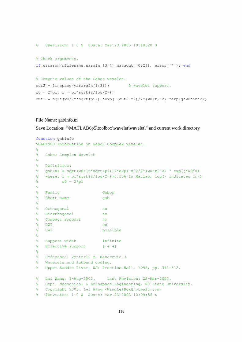
118
% $Revision: 1.0 $ $Date: Mar.23,2003 10:10:20 $
% Check arguments.
if errargn(mfilename,nargin,[3 4],nargout,[0:2]), error('*'); end
% Compute values of the Gabor wavelet.
out2 = linspace(varargin1:3); % wavelet support.
w0 = 2*pi; r = pi*sqrt(2/log(2));
out1 = sqrt(w0/(r*sqrt(pi)))*exp(-(out2.^2)/2*(w0/r)^2).*exp(j*w0*out2);
File Name: gabinfo.m
Save Location: “\MATLAB6p5\toolbox\wavelet\wavelet\” and current work directory
function gabinfo
%GABINFO Information on Gabor Complex wavelet.
%
% Gabor Complex Wavelet
%
% Definition:
% gab(x) = sqrt(w0/(r*sqrt(pi)))*exp(-x^2/2*(w0/r)^2) * exp(j*w0*x)
% where: r = pi*sqrt(2/log(2))=5.336 In Matlab, log() indicates ln()
% w0 = 2*pi
%
% Family Gabor
% Short name gab
%
% Orthogonal no
% Biorthogonal no
% Compact support no
% DWT no
% CWT possible
%
% Support width infinite
% Effective support [-4 4]
%
% Reference: Vetterli M. Kovacevic J,
% Wavelets and Subband Coding.
% Upper Saddle River, NJ: Prentice-Hall, 1995, pp. 311-312.
% Lei Wang, 8-Aug-2002. Last Revision: 23-Mar-2003.
% Dept. Mechanical & Aerospace Engineering, NC State University.
% Copyright 2003. Lei Wang <[email protected]>
% $Revision: 1.0 $ $Date: Mar.23,2003 10:09:56 $

119
A.4 Bandwidth of a Signal
There are several ways in which bandwidth can be defined, but two common
approaches are often used to evaluate the bandwidth of a signal. One is 3-dB bandwidth
which is widely used in signal processing; the other is based on the standard deviation that is
usually used in mathematics since it can give the bandwidth from the analytical spectrum
expression of the signal.
A.4.1 3-dB bandwidth
3-dB bandwidth may be the simplest definition and it is suitable for the signal without
the need of analytical spectrum expression. If maxs is the maximum amplitude of the
frequency spectrum of a signal )(ˆ ωs , and considering the power is proportional to the square
of amplitude, the amplitude at which the power of the signal is half that of the peak is given
by (Orfanidis, 1996)
2ˆˆ 2max
2 ss powerhalf =− (A.4-1)
where 2maxs is the maximum power of the signal and 2ˆ powerhalfs − is half of the maximum power.
In dB, this condition reads
dB3)21log(10)ˆ
ˆlog(20
max
−==−
s
s powerhalf (A.4-2)
Therefore, the amplitude associated with the half-power points of a signal is dB3
below the maximum value. On a linear scale of amplitude, the amplitude at a half-power
point is given by
maxmax ˆ707.0ˆ2
2ˆ sss powerhalf ≈=− (A.4-3)

120
Therefore 3-dB bandwidth s∆ is the frequency bandwidth between the half-power
points of the spectrum.
Consider the Gabor function Eq. (3.2-2) and the relation Eq. (A.4-3), the following
equation can be obtained
2
2])(
2
)(exp[ 2
0
20 =−− ωωωγ
(A.4-4)
Solving Eq. (A.4-4), the frequency coordinates of two half-power points are
2ln00 γωωω ±=−powerhalf (A.4-5)
Thus the 3-dB bandwidth of the Gabor function is
2ln2)(ˆ 0
γωωψ =∆ g (A.4-6)
Especially, if 2ln2πγ = and πω 20 = , then 1.3863)(ˆ =∆ ωψ g .
Figure A.2 shows the parameters associated with 3-dB bandwidth of Gabor function.
0 1 2
0
1
2
ω/(2π)
Ψg( ω
)
maxˆ707.0ˆgpowerhalfg ψψ ×=−
maxˆ gψ
)(ˆ ωψ g∆
powerhalf −ωpowerhalf −ω
Figure A.2 Illustration of 3-dB bandwidth of Gabor function 1.3863)(ˆ =∆ ωψ g

121
A.4.2 Standard deviation bandwidth
If the analytical spectrum expression of signal )(ts is known, say )(ˆ ωs , its frequency
bandwidth s∆ can be also derived from the standard deviation of )(ˆ ωs (Mallat, 1998).
∫∞+
∞−−= ωωωω
πσ ds
tscs
222
2ˆ )(ˆ)(
)(2
1 (A.4-7)
where )(ˆ ωs is the Fourier transform of the signal, cω is the central frequency of the function
)(ˆ ωs . Then bandwidth is defined as
ss ˆˆ σ=∆ (A.4-8)
For the Gabor function, since 1)( =tgψ , )(ˆ)(ˆ ωψωψ gg = , and its central frequency
equals to 0ω , Eq. (A.4-7) can be rewritten as
∫
∫∞+
∞−
∞+
∞−
−−−=
−−−=
ωωωωγωω
ωγ
π
ωωωωγ
ωγ
ππωω
πσ ωψ
d
dg
])()(exp[)(1
])()(exp[2
)(2
1
20
2
0
20
0
20
2
00
20
2)(ˆ
(A.4-9)
Considering the following known integral
πpp
pdxex px
2)(2 )sgn(
2
12
=∫∞+
∞−
− (A.4-10)
where p is a real constant. Then, Eq. (A.4-9) can be simplified as
4
00
2)(ˆ
2ln82
1 πωγωσ ωψ ==
g (A.4-11)
Thus the corresponding bandwidth of Gabor function is
8
40
)(ˆ2ln8
)(ˆπω
σωψ ωψ ==∆gg (A.4-12)
Especially, if πω 20 = , then 1.7015)(ˆ =∆ ωψ g .

122
0 1 2
0
1
2
ω/(2π)
Ψg( ω
))(ˆ ωψ g∆
Figure A.3 Illustration of standard deviation bandwidth of Gabor function 1.7015)(ˆ =∆ ωψ g
A.5 Derivation of Eq. (3.4-10) from Eq. (3.4-9)
Eq. (3.4-9) can be rearranged as
∫∞+
∞−−= ωωωψω
πdkxbiaF
aba gw )](exp[)(ˆ)(ˆ
2),(WT (A.5-1)
where )(ˆ ωψ ag is a real-valued Gaussian function given by
])(2
)(exp[
2)(ˆ 2
0
20
04
ωωωγωγ
ππωψ −−= aag
Central frequency and bandwidth of )(ˆ ωψ ag are given by ac 0ωω = and
aa gg )(ˆ)(ˆ ωψωψ ∆=∆ , where 0ω and )(ˆ ωψ g∆ are the central frequency and standard
deviation bandwidth of the Gabor function )(ˆ ωψ g defined in Appendix A.4.2, respectively.
Thus )(ˆ ωψ ag may be considered as a band-pass filter and its central frequency is at cω .
In the following, a function is defined as
)()( kxbi −= ωωϕ (A.5-2)

123
Functions )(ωϕ and )(ˆ ωF in Eq. (A.5-1) can be expanded at the central
frequency cωω = of )(ˆ ωψ ag by using a first-order Taylor expansion in the vicinity of
ac 0ωω = .
))(()()( ccc ωωωϕωϕωϕ −′+≈
))(( cc xkbiikxbi ωωω −′−+−=
ωω )()( xkbikkix c ′−+−′= (A.5-3)
where ωωω ddkk cc /)()( =′ .
Similarly,
ωωωωωωωωωω )(ˆ)(ˆ)(ˆ))((ˆ)(ˆ)(ˆccccccc FFFFFF ′+′−=−′+≈ (A.5-4)
where ωωω dFdF cc )(ˆ)(ˆ ′=′
Letting )(1 kkixc c −′= ω and )(ˆ)(ˆ2 ccc FFc ωωω ′−= , Eq. (A.5-1) becomes
∫∞+
∞−′−+′+= ωωωψωω
πdxkbicaFc
aba gcw ])(exp[)(ˆ])(ˆ[
2),(WT 12 (A.5-5)
The integration above can be conveniently evaluated as a sum of the two terms, 1I
and 2I by splitting the term in the first square bracket in the integrand into two parts. In
addition, since both 1c and 2c are not functions of ω , they can be placed outside of the
integration. Starting from the first term I1,
∫∞+
∞−′−+= ωωωψ
πdxkbicac
aI g ])(exp[)(ˆ
2 121
∫∞+
∞−′−= ωωωψ
πdxkbiac
acg ])(exp[)(ˆ)exp(
2 12

124
∫∞+
∞−
′−=a
ad
a
xkbiaac
acg
)()exp()(ˆ)exp(
2 12 ωωωψπ
(A.5-6)
Using the inverse Fourier transform ( ) )(exp)(ˆ tdit gg ψξξξψ =∫∞+
∞−, the equation above
can be simplified as
)exp()(2
12
1 ca
xkb
a
cI g
′−= ψπ
(A.5-7)
Plugging 1c and 2c into the equation above leads to
)](exp[)(2
)(ˆ)(ˆ1 kkix
a
xkb
a
FFI cg
ccc −′′−′−= ωψπ
ωωω (A.5-8)
Following a similar approach, the second term of the integration, I2, is
∫∞+
∞−′−′= ωωωψωω
πdxkbiaFc
aI gc ])(exp[)(ˆ)(ˆ)exp(
2 12
∫∞+
∞−
′−′= )(]exp[)(ˆ)()exp(
2
)(ˆ12
ωωωψωπ
ωad
a
xkbiaaaic
ia
aFg
c (A.5-9)
Knowing the inverse Fourier transform relationship ( ) )(exp)(ˆ tditi gg ψξξξψξ ′=∫∞+
∞−,
we have
)]2(exp[)(2
)(ˆ22 πωψπ
ω −−′′−′′= kxxki
a
xkb
a
aFI cg
c (A.5-10)
In summery, the first-order Taylor series expansion of the Eq. (A.5-1) leads to the
resulting form of Eq. (3.4-10) given by
)()]2(exp[2
)(ˆ
)()](exp[(2
)(ˆ)(ˆ),(WT
2 a
xkbkxxki
a
Faa
xkbkxxki
a
FFba
gcc
gcccc
w
′−′−−′′+
′−−′′−=
ψπωπω
ψωπ
ωωω
(A.5-11)

125
A.6 Source Localization using Triangulation Method
In this Appendix, a triangulation method for passive source localization is introduced
from time differences of arrival (TDOA’s) between pairs of sensors and sensor locations. In
isotropic plates, closed-form solutions can be given when the number of TDOA
measurements is equal to the number of unknowns (r and θ). However, for anisotropic plates
where the group velocity is dependent on the wave propagation direction, an iterative
algorithm needs to be developed to identify the source location.
A.6.1 Isotropic plates
To uniquely locate the impact source in a plate, measurements from three sensors
must be used. Tobias (1976) formulated the problem by identifying the source location as
three intersecting circles, each centered at a sensor, with their radii determined by the time of
propagation of the wave emitted from the source to the respective sensor. Without loss of
generality, sensor 0S is taken at the origin of the coordinate. Two other sensors 1S and 2S are
located at ),( 11 yx and ),( 22 yx respectively. By solving the three resulting equations
simultaneously, closed-form solutions for the source location can be expressed by the
radius r , measured from a sensor located at a reference origin, and the angleθ measured
counter-clockwise from the x-axis. Figure A.4 shows a source location relative to the three
sensors.

126
1δ+r
2δ+r
r
θ
Figure A.4 Source localization by triangulation method for an isotropic plate
The impact source at P(x, y) is located at the point of intersection of the circles about
S0, S1, and S2 as centers with radii r , 1δ+r , and 2δ+r respectively.
The equations of the three circles are written respectively as:
222 ryx =+ (A.6-1a)
21
21
21 )()()( δ+=−+− ryyxx (A.6-1b)
22
22
22 )()()( δ+=−+− ryyxx (A.6-1c)
Substituting the first equation into the last two equations leads to
)(222 21
21
21111 δ−+=δ++ yxryyxx (A.6-2a)
)(222 22
22
21222 δ−+=δ++ yxryyxx (A.6-2b)
Changing the variables x and y in the polar coordinates in the above equation gives
1111 )sincos(2 Ayxr =++ δθθ (A.6-3a)

127
2222 )sincos(2 Ayxr =++ δθθ (A.6-3b)
where 21
21
211 δ−+= yxA and 2
222
222 δ−+= yxA . Note that if the source location does not
coincide with the reference sensor location, 1A and 2A are not equal to zero. Then from Eq.
(A.6-3) 0sincos 111 ≠++ δθθ yx and 0sincos 222 ≠++ δθθ yx .
1δ and 2δ contained in Eq. (A.6-3) and A1 and A2 can be calculated from
gct11 ∆=δ and gct22 ∆=δ (A.6-4)
where gc is the group velocity and 1t∆ and 2t∆ are the time differences of arrival (TDOA’s)
at sensor pairs 10 , SS and 20 , SS respectively.
For 0sincos 111 ≠++ δθθ yx and 0sincos 222 ≠++ δθθ yx , the radius r can be
determined by
)sincos(2)sincos(2 222
2
111
1
δθθδθθ ++=
++=
yx
A
yx
Ar (A.6-5)
Using Eq. (A.6-5) the following identify can be deduced:
211212211221 sin)(cos)( δ−δ=θ−+θ− AAyAyAxAxA (A.6-6)
Dividing the term 2/121221
21221 ])()[( yAyAxAxAB −+−= on both sides of Eq. (A.6-
6) and defining
B
AAK 2112 δδ −= (A.6-7)
the angle θ can be solved by the following equation
K=− )cos( φθ (A.6-8)
where 1221
1221tanxAxA
yAyA
−−=φ .

128
Since the numerator and denominator of φtan , parameters B and K can be
determined from the known positions of the two sensors 1S and 2S , the time differences of
arrival 1t∆ and 2t∆ , and group velocity gc , the angle can be determined first by
K1cos−+=φθ (A.6-9)
Using Eq. (A.6-5) with Eq. (A.6-9) the radius r can be then determined. Then the
single damage can be localized by knowing the two unknowns r and θ .
A.6.2 Summary of the triangulation method (Tobias, 1976)
• The method is not an active detection technique but a passive sensing method,
unsuitable for structural health monitoring;
• Three sensors can be placed in arbitrary triangle;
• The method is only suitable for isotropic plates due to the assumption of constant
group velocity gc ;
• The method can localize the source outside of the triangular area;
• Two unknowns ),( θr are the source location in polar coordinates. Knowing ),( θr ,
the source location in the Cartesian coordinates can be simply obtained by θcosrx =
and θsinry = ;
• The following parameters are given for locating the impact source:
o Geometry parameters: the Cartesian coordinates of three sensors
)0,0(0 S , ),( 111 yxS , and ),( 222 yxS ;
o Measured parameters: 1t∆ and 2t∆ are the time differences of arrival (TDOA’s)
at the sensor pairs 10 , SS and 20 , SS respectively;
o Constant group velocity: gc ;

129
In majority of the cases, the solution for the source location ),( θr is unique. However, in
few exceptional cases, there exist two physical solutions for ),( θr . Such solutions are so-
called ambiguous solutions (Tobias, 1976). In order to resolve the ambiguous solutions it
is necessary to use a fourth sensor 3S , located at the point ),( 33 yx .
A general procedure of locating the impact source can be taken by the following steps:
1. Calculate φ first by knowing 1t∆ and 2t∆ and sensor locations;
2. Compute the unknownθ by Eq. (A.6-9). Note that since θ has two solutions
over the range ),( ππ− where two solutions of θ are obtained;
3. Use the two values of θ to calculate the unknown radius r with Eq. (A.6-5).
Neglect the inadmissible angleθ if the corresponding 0<r . Then obtain the
unique solution for the source location ),( θr ;
4. Transfer ),( θr to Cartesian coordinate system θcosrx = and θsinry = .
A.6.3 Anisotropic plates
Since the group velocity of wave propagating in an anisotropic plate is not constant
but depends on the propagation direction, the proposed method in the above section is not
valid for anisotropic plates. For a planar source location, three sensors must be used.
Analysis of arrival times at different sensors enables the emission source to be located by
means of a triangulation method. A pair of differences in the arrival time from an array of
three sensors defines two hyperbolae at which point of intersection the emission source is
located. For isotropic materials, a closed form solution has been derived (Tobias, 1976). In
anisotropic materials, the source location determination becomes more complicated since the
group velocity is function of direction of propagation in the plate.

130
2l
0θ
1θ1l
φ
α
2θ
0r
2r
1r
3l
Figure A.5 Source localization analysis for an anisotropic plate
Figure A.5 shows three sensors 0S , 1S , and 2S and the location of a source
),( yxP relative to the sensors. Three wave propagating directions from the impact source are
as follows: PS0 (direction: φπθ ++0 ), PS1 (direction: φθπ +− 12 ), and PS2 (direction:
φαθ ++2 ). Since the group velocity of wave is function of both propagation direction and
frequency f , three group velocities may be expressed as:
),( 00 fcc gg φπθ ++= (A.6-10a)
),2( 11 fcc gg φθπ +−= (A.6-10b)
),( 22 fcc gg φαθ ++= (A.6-10c)
Sensors 0S and 1S are considered first. The time difference of arrival (TDOA) at the
sensor pair 10 , SS is
0
0
1
1011
gg c
r
c
rttt −=−=∆ (A.6-11)

131
From geometric considerations, the unknown distances 1r and 0r can be written in
terms of the unknown angles and the known distance between 1S and 0S .
From sine law, we have the following relation in the triangle PS0S1
1
10
0
1
1
0 )sin(sinsin
lrr
θθθθ +== (A.6-12)
Then the distances 0r and 1r can be expressed as
+=
+=
)sin(
sin)sin(
sin
10
011
10
110
θθθθθθ
lr
lr
(A.6-13)
Plugging Eq. (A.6-13) back into Eq. (A.6-11) gives
1100
11
101
01
)sin(
sin
)sin(
sint
c
l
c
l
gg
∆=+
−+ θθ
θθθ
θ (A.6-14)
Because the analytical expression of gc is not available for anisotropic plates and only
the numerical values of gc with different wave propagating directions can be obtained, it is
unlikely to obtain the analytical solution to Eq. (A.6-14). Thus a numerical method is
employed to get the solution.
In order to solve Eq. (A.6-14) numerically, we can rearrange the equation and define
the following cost function 1J to avoid possible denominator to vanish and to make the
computation more stable.
)sin(sinsin 101011110011 θθθθ +∆−−= gggg cctclclJ (A.6-15)
For a fixed value 0θ , 1θ is iterated through to calculate the values of cost function 1J
until 1J approaches zero and usually less than a specified terminal error. At this end, the

132
solution 1θ from Eq. (A.6-15) is obtained for the fixed 0θ . Next a sufficiently small step size
change 0θ is made and the same iteration above to search another 1θ is performed. After
searching the suitable values of 0θ and 1θ , the source possible location of ),( yxP may be
expressed as
++
=+=
++
=+=
)sin()sin(
sin)sin(
)cos()sin(
sin)cos(
010
1100
010
1100
φθθθθφθ
φθθθθφθ
lry
lrx
(A.6-16)
This produces locus of possible location points. Physically, all the points on the loci
satisfy the arrival time difference 1t∆ at the sensor pair 10 , SS .
In a similar manner, from sine law, we have the following relation in the triangle
PS0S2
2
20
0
2
2
0 )sin(sin)sin(
lrr
θθαθθα +−==
− (A.6-17)
The distances 0r and 2r can then be written as
+−−=
+−=
)sin(
)sin()sin(
sin
20
022
20
220
θθαθαθθα
θ
lr
lr
(A.6-18)
The time difference of arrival 2t∆ at the sensor pair 20 , SS .
0
0
2
2022
gg c
r
c
rttt −=−=∆ (A.6-19)
Plugging Eq. (A.6-18) into Eq. (A.6-19) yields
2200
22
202
02
)sin(
sin
)sin(
)sin( δθθα
θθθα
θα=
+−−
+−−
gg c
l
c
l (A.6-20)

133
Similarly, define the cost function J2 as
)sin(sin)sin( 202022220022 θθαθθα +−∆−−−= gggg cctclclJ (A.6-21)
Use the iterative procedures to search the solution 0θ and 2θ which make the cost
function 2J approaches zero. After searching the suitable values of 0θ and 2θ , the possible
source location of ),( yxP may be obtained as
++−
=+=
++−
=+=
)sin()sin(
sin)sin(
)cos()sin(
sin)cos(
020
2200
020
2200
φθθθα
θφθ
φθθθα
θφθ
lry
lrx
(A.6-22)
The produces locus of possible location points, which satisfy the TDOA equals to
2t∆ . The intersection of the two loci is the source location (Jeong and Jang, 2000).
A.6.4 Summary of the triangulation method (Jeong and Jang, 2000)
• The method is not an active detection technique but a passive sensing method,
unsuitable for structural health monitoring;
• Three sensors can be arranged in arbitrary triangle;
• The method can locate the source either in an isotropic or in an anisotropic plate;
• The valid detection area includes within and beyond the enclosed triangular area;
• The closed-form solution of source location is not available because the closed-form
expression of group velocity are inaccessible for anisotropic plates;
• The method can only obtain the numerical solution and a graphic technique is used to
search the intersection of the two loci, the finial resulting location;
• Using the vector computation technique instead of do-loop in Matlab®, the
computation speed is acceptable. For example, it takes less than 20 seconds to get the

134
source location in IM6/3501-6 composite plate by using a computer with 1.5GHz and
256MB RAM.
A.6.5 Numerical Simulation
This section demonstrates numerical simulation results of single source localization in
both aluminum and composite plates based on Jeong and Jang’s (2000) triangulation method
by using two TDOA values. Three sensors are located at (0, 0)m, (10, 2)m, and (2, 10)m in a
plate. Table 2.1 and Table 3.1 list the material properties of IM7/5250-4 composite plate and
Al 6061 aluminum plate, respectively. After knowing the distance from source to sensor and
calculating the group velocity, the time-of-flight of wave propagating from the source to the
sensor can be theoretically computed; then the TDOA of sensor S1 and S2, and TODA of
sensor S1 and S3 are obtained. Finally, these two TDOA values are fed into the algorithm of
Section A.6.3 to numerically search the source location.
In the following figures, the green circles are the location of three sensors, and the red
“x” indicates the location of target source. In addition, the blue locus denotes the possible
source location which satisfies the TODA of sensor S1 and S2. Similarly, the cyan locus is the
possible source location for the TODA of sensor S1 and S3. The evaluated source location is
located at the cross point of the two loci in each figure.

135
−4 −2 0 2 4 6 8 10 12 14−4
−2
0
2
4
6
8
10
12
14
S1
S2
S3
x (m)
y (m
)
Triangulation Source Location for Composite Plate (IM7/5250−4)
Figure A.6 Numerical simulation of source location in anisotropic plate with source at (6, 4) m
denoted by “x”
−4 −2 0 2 4 6 8 10 12 14−4
−2
0
2
4
6
8
10
12
14
S1
S2
S3
x (m)
y (m
)
Triangulation Source Location for Isotropic Plate (Al6061−T6)
Figure A.7 Numerical simulation of source location in isotropic plate with source at (6, 4) m denoted
by “x”

136
−4 −2 0 2 4 6 8 10 12 14−4
−2
0
2
4
6
8
10
12
14
S1
S2
S3
x (m)
y (m
)
Triangulation Source Location for Composite Plate (IM7/5250−4)
Figure A.8 Numerical simulation of source location in anisotropic plate with source at (10, 10) m
denoted by “x”
−4 −2 0 2 4 6 8 10 12 14−4
−2
0
2
4
6
8
10
12
14
S1
S2
S3
x (m)
y (m
)
Triangulation Source Location for Isotropic Plate (Al6061−T6)
Figure A.9 Numerical simulation of source location in isotropic plate with source at (10, 10) m
denoted by “x”