eindhoven university of technology master … we develop algorithms for detecting the moving-along...
TRANSCRIPT

Eindhoven University of Technology
MASTER
Detecting the moving-along pattern in trajectory data
Li, T.
Award date:2012
DisclaimerThis document contains a student thesis (bachelor's or master's), as authored by a student at Eindhoven University of Technology. Studenttheses are made available in the TU/e repository upon obtaining the required degree. The grade received is not published on the documentas presented in the repository. The required complexity or quality of research of student theses may vary by program, and the requiredminimum study period may vary in duration.
General rightsCopyright and moral rights for the publications made accessible in the public portal are retained by the authors and/or other copyright ownersand it is a condition of accessing publications that users recognise and abide by the legal requirements associated with these rights.
• Users may download and print one copy of any publication from the public portal for the purpose of private study or research. • You may not further distribute the material or use it for any profit-making activity or commercial gain
Take down policyIf you believe that this document breaches copyright please contact us providing details, and we will remove access to the work immediatelyand investigate your claim.
Download date: 12. Jun. 2018

TECHNISCHE UNIVERSITEIT EINDHOVENDepartment of Mathematics and Computer Science
Detecting the Moving-Along Patternin Trajectory Data
ByT. Li
Supervisors:
dr. M. E. Buchinprof. dr. B. Speckmann
Eindhoven, July 2012


Abstract
We develop algorithms for detecting the moving-along pattern in trajectory data. Given atrajectory of a moving entity and a subdivision of the space it moves in, we want to find thesub-trajectories where the moving entity moves along the subdivision boundaries. We use theFrechet distance to partially match the trajectory and the subdivision boundary. We presentdifferent scenarios of a moving entity and the subdivision boundary and show how they canbe handled by the free space diagram, the geometric data structure for computing the Frechetdistance.
We develop an algorithm based on a variant of the Frechet distance, the weak Frechetdistance, to discover sub-trajectories along the subdivision boundaries. We use jumps tomerge overlapping sub-trajectories. We give an O(mn logm) algorithm to find all jumps inthe free space diagram with the help of a balanced binary tree.
We apply the model to study the movement pattern of gulls flying along the coastline.We implement the algorithms and test them on gull data sets.
3


Contents
1 Introduction 71.1 Problem Description . . . . . . . . . . . . . . . . . . . . . . . . . . . . . . . . 81.2 Case Study . . . . . . . . . . . . . . . . . . . . . . . . . . . . . . . . . . . . . 81.3 Related Work . . . . . . . . . . . . . . . . . . . . . . . . . . . . . . . . . . . . 91.4 Overview . . . . . . . . . . . . . . . . . . . . . . . . . . . . . . . . . . . . . . 10
2 Frechet Distance 112.1 Definition for Frechet Distance . . . . . . . . . . . . . . . . . . . . . . . . . . 112.2 Free Space Diagram . . . . . . . . . . . . . . . . . . . . . . . . . . . . . . . . 112.3 Deciding the Frechet Distance . . . . . . . . . . . . . . . . . . . . . . . . . . . 12
3 Problem Definition 133.1 Preliminary . . . . . . . . . . . . . . . . . . . . . . . . . . . . . . . . . . . . . 133.2 Definition of Moving-along Pattern . . . . . . . . . . . . . . . . . . . . . . . . 133.3 Similarity Measures . . . . . . . . . . . . . . . . . . . . . . . . . . . . . . . . 143.4 Scenario Analysis . . . . . . . . . . . . . . . . . . . . . . . . . . . . . . . . . . 15
4 Algorithm 214.1 Main Algorithm . . . . . . . . . . . . . . . . . . . . . . . . . . . . . . . . . . . 214.2 Algorithm to Find Jumps . . . . . . . . . . . . . . . . . . . . . . . . . . . . . 214.3 Find Nearest Jump with a Balanced Binary Tree . . . . . . . . . . . . . . . . 264.4 Non-monotone Jumps . . . . . . . . . . . . . . . . . . . . . . . . . . . . . . . 32
5 Implementation 35
6 Experiments 376.1 Experimental Setting for Synthetic Data . . . . . . . . . . . . . . . . . . . . . 376.2 Results for Synthetic Data Experiments . . . . . . . . . . . . . . . . . . . . . 376.3 Experimental Setting for Real Data . . . . . . . . . . . . . . . . . . . . . . . . 416.4 Results for Real Data Experiments . . . . . . . . . . . . . . . . . . . . . . . . 42
7 Conclusion 49
A Visualized Results in Google Earth 51
B Jumps in Real Data 57
5


Chapter 1
Introduction
As tracking technology advances, especially with the development of high-resolution GPS andother remote sensing techniques, more and more movement data become available. In partic-ular, animal movement data are collected for the study of animal ecology. The data record thefixes of an animal within a period of time, and possibly some physiological parameters (e.g.heart rate, body temperature, breath rate, etc) or environmental parameters (such as windspeed/direction, humidity, etc). Researchers then analyze these data to explain the animal’smovement patterns and behaviors. Such studies are important for evaluating the conservationstatus of a species, and for understanding how human activity influences its habits.
Traditionally, the data analysis on this type of data is executed manually. With the in-creasing amount of movement data, it becomes impractical to process these data entirely byhand. Therefore researchers today develop algorithms to efficiently perform analysis tasks onthese data. Some typical data analysis tasks are trajectory segmentation, trajectory cluster-ing, movement pattern mining and trajectory visualization.
In this thesis we study detecting the moving-along pattern in trajectory data. That is,we are given the trajectory of a moving entity and a subdivision of the space it moves in.Our task is to find the sub-trajectories where the moving entity was moving along subdivisionboundaries. Such pattern of moving along the boundaries can be frequently found in the realworld, such as pedestrians walking along the street, monkeys moving along the forest edge,pigeons flying along the roads, etc. In our research the application scenario is gulls flyingalong the coastline.
We study the movement of Lesser Black-backed Gulls (Larus fuscus) with breeding colonyon Texel island, the Netherlands. The research on these gulls is a long-term study of gullbehavior carried out by the CGE-Group (Computational Geo-Ecology) at UvA. The studyaims at a better understanding of the foraging movement patterns of the gulls and theirbehavior outside the colony.
It is known that these gulls move in an irregular cyclic pattern with their colony asstart and end point of each trip [23]. In most times the travel path over sea is counter-clockwise: the gull leaves the nest towards west and returns with direction towards east ornortheast. Sometimes the returning paths are exactly along the coast. Ecologists want tofind the relationship between such “moving-along-coastline” pattern and the cyclic movementpattern. To do this the gull paths that are along the coastline need to be discovered, whichis the main task in this thesis.
7

T. Li
1.1 Problem Description
Given the trajectory of a moving entity and a subdivision of the region it moves in, we want todevelop an algorithm to report all sub-trajectories that are along the subdivision boundaries.In our research we apply this algorithm to finding the gull sub-trajectories that are along thecoastline. It can also be applied to other real world scenarios as described above.
In Figure 1.1 we give an example to illustrate the problem. The trajectory of the movingentity is presented as an arrowed line; the subdivision boundaries are presented as thickergrey curves. The highlighted part between two points is the sub-trajectory where the movingentity was moving along the subdivision boundary.
Subdivision boundary
Trajectory of moving entity
Figure 1.1: An example of entity moving along the subdivision boundary
1.2 Case Study
The moving entities we study are lesser black-backed gulls. The gull data set contains theGPS records of 8 lesser black-backed gulls (four adult males and four adult females) fromJune 1st to June 30th, 2010. The data were collected using the UvA Bird Tracking System[22]. Each gull has a unique ID and its nest location is recorded. A circular region centeredat the nest location with 200m radius is regarded as the gull’s colony [22]. Each GPS recordin the data set consists of the date and time, longitude, latitude, x/y coordinates (projectedto RD-new Dutch coordinates 1), altitude, sensor temperature, GPS speed and the distanceto the colony center.
The subdivision boundary in our case study is the coastline. We obtained the coastlinedata from National Geophysical Data Center (NGDC). The data set is derived from theGlobal Self-consistent, Hierarchical, High-resolution Shoreline Database (GSHHS) [25] withhigh resolution. Each sample point of the coastline is represented by latitude and longitude.We convert the latitude and longitude of each point to x/y coordinates in RD-new Dutchcoordinate system for geometry computations.
1http://www.cachemaps.com/Downloads.php. Accessed on 25 May, 2012
8

Detecting the Moving-Along Pattern in Trajectory Data
1.3 Related Work
Recently there has been extensive research in the area of computational movement analysis.Many different tasks are performed to analyze trajectory data. Gudmundsson et al. [15]present an overview of movement data and survey theories and applications for movementdata analysis.
Trajectory clustering is a common trajectory analysis task. Often similar trajectories asa whole are grouped to discover common trajectories. Lee et al. [20] provide a density-basedclustering algorithm to analyze hurricane movement data and animal trajectory data. Fu etal. [14] analyze vehicle motion trajectories with a two-layer hierarchical clustering algorithm.Gudmundsson et al. [17] use clustering techniques to analyze football player trajectories in amatch. Buchin et al. [8] use partial clustering to detect commuting pattern.
Another trajectory analysis task is trajectory segmentation. It partitions a trajectoryinto semantically meaningful segments. Buchin et al. [9] present an algorithmic framework tosegment a trajectory into segments of similar movement characteristics, such that the numberof segments is minimal. Rasetic et al. [21] , Anagnostopoulos et al. [2] use minimum boundingboxes to segment a trajectory to support efficient search operations and range queries.
Movement pattern mining studies patterns in the movement behavior of moving entities.Dodge et al. [11] propose a conceptional framework to define movement behavior and es-tablish a categorization of movement patterns. Some typical movement patterns of movingentities are: leadership pattern (Andersson et al. [3]), single file (Buchin et al. [7]), flock(Gudmundsson et al. [16]) and commuting pattern (Buchin et al. [8]).
Movement analysis is also combined with visualization. Dykes et al. [13] survey a numberof graphical techniques and representation methods for movement data. Andrienko et al. [4]use visual analytics to analyze massive collections of movement data.
In particular, our research is related to measuring the similarity between two trajectories.Various works have been done on this topic. Several approaches are based on techniques insequence analysis. For example, Chen et al. [10] introduce Edit Distance on real sequences(EDR) to measure the similarity between two trajectories. Dynamic Time Warping (DTW)has been also applied to measure the similarity in time-series data [18, 19]. The LongestCommon Subsequence (LCSS) is another similarity measure for sequences. Vlachos et al. [24]present efficient techniques to compute trajectory similarity based on the LCSS model.
Several approaches compute the similarity between trajectories based on their geometry.The most relevant similarity measures of this type for our research are avg/max equal timedistance, the Hausdorff distance and the Frechet distance. Yanagisawa et al. [26] present anefficient indexing method to perform similarity queries for trajectory data based on average-equal-time distance. Biliotti et al. [5] propose a clustering algorithm to count the number ofpedestrians given a trajectory data set based on the Hausdorff distance. Brakatsoulas et al. [6]present map-matching algorithms to analyze vehicle movement data based on the Frechet dis-tance. Buchin et al. use the Frechet distance to detect the single file movement pattern [7] andcommuting pattern [8]. In Section 3.3 we will discuss these three similarity measures in detail.
The Frechet distance has several variants. Alt and Godau introduce the weak Frechetdistance in [1]. In our work we will use the weak Frechet distance. Driemel et al. [12] studythe Frechet distance with shortcuts and give a near linear time approximation algorithm forc-packed input curves. We develop an algorithm for the Frechet distance with jumps whichis closely related to the algorithm of Driemel et al.. We will introduce the Frechet distancein Chapter 2.
9

T. Li
1.4 Overview
The thesis is organized as follows. In Chapter 2 we introduce the Frechet distance whichwill be the basis of our work. In Chapter 3 we give a model for the problem and show howwe handle different possible scenarios. In Chapter 4 we present algorithms to find the sub-trajectories that are along the subdivision boundary. In Chapter 5 we show the structureof the implementation. In Chapter 6 we introduce the experiments conducted and show theresults. In Chapter 7 we give conclusions and propose directions for further research.
10

Chapter 2
Frechet Distance
In this chapter we introduce an important similarity measure which will be the basis of ourresearch.
2.1 Definition for Frechet Distance
The Frechet distance measures the similarity of two parameterized curves. The study ofthe Frechet distance from the view of computational geometry was initialized by Alt andGodau [1]. Formally, let τ1 and τ2 be two parameterized curves τ1(α(t)) and τ2(β(t)), whereα(t) and β(t) are non-decreasing continuous functions of parameter t ∈ [0, 1], such thatα(0) = β(0) = 0 and α(1) = β(1) = 1. Then the Frechet distance between τ1 and τ2 isdefined as:
δF (τ1, τ2) = infα : [0, 1] → [0, 1]β : [0, 1] → [0, 1]
maxt∈[0,1]
d
(τ1
(α(t)
), τ2
(β(t)
))Here d(·) denotes the distance between two points. The Frechet distance is a common simi-larity measure for computing trajectory similarity [6, 7].
The weak Frechet distance is a variant of the Frechet distance. It is defined in the sameway with the Frechet distance except that the parameterizations α(t) and β(t) can be non-monotonic functions [1], so it is also called non-monotone Frechet distance.
2.2 Free Space Diagram
To compute the Frechet distance one commonly uses the free space diagram. Assume weare given two line segments P and Q parameterized over [0, 1], i.e. P and Q are continuousfunctions P : [0, 1]→ R2 and Q : [0, 1]→ R2. We are also given a distance parameter ε > 0.The free space of P and Q is defined as
Fε(P,Q) =
{(x, y) ∈ [0, 1]2 | d
(P (x), Q(y)
)≤ ε}
where d(·) denotes the distance between two points. Fε describes all the point pairs (P (x), Q(y))whose distance is at most ε. Now we extend P and Q to polygonal curves with arbitrarynumber of line segments, say P consists of n segments and Q consists of m segments:
Fε(P,Q) =
{(x, y) ∈ [0, n]× [0,m] | d
(P (x), Q(y)
)≤ ε}
11

T. Li
Such an n ×m diagram together with Fε is known as the free space diagram Dε(P,Q). InDε(P,Q) every vertical line corresponds to a vertex of P and every horizontal line correspondsto a vertex of Q. Every pair of line segments, one from P and one from Q, defines a free spacecell Cij , which corresponds to the ith segment of P and the jth segment of Q.
Ivij
Ihij
Ivi+1j
Ihij+1
Fε
Cij
Fε
LFij
RFij
Cij
(a) (b)
Figure 2.1: Free Space Cell
We define the interval Ivij as the intersection segment of Fε and the left boundary of
Cij . The interval Ihij is the intersection segment of Fε and the bottom boundary of Cij , seeFigure 2.1(a). If Fε ∩ Cij 6= ∅, we define:
• RFij - the maximum x-coordinate of all points on Fε ∩ Cij . RFij ∈ [i, i+ 1].
• LFij - the minimum x-coordinate of all points on Fε ∩ Cij . LFij ∈ [i, i+ 1).
In Figure 2.1(b) we show RFij and LFij in a free space cell. Given the definition we know that
if Ivij 6= ∅, then LFij = i; if Ivi+1j 6= ∅, then RFij = i + 1. From the view of geometry, for any
point p ∈ P (i, LFij) ∪ P (RFij , i+ 1) and any point q ∈ Q(j, j + 1), d(p, q) > ε. Here P (·), Q(·)denote the sub-curve of P and Q. We further define the interval IFij = [LFij , R
Fij ]. If a free
space cell Cij has non-empty right boundary Ivi+1j 6= ∅, we say Cij is a live cell. We will usethis concept in the analysis in Section 4.2.
2.3 Deciding the Frechet Distance
The decision problem of the Frechet distance is defined as: given two polygonal curves P andQ, and a parameter ε, decide whether δF (P,Q) ≤ ε. Alt and Godau [1] showed that given Pwith n segments and Q with m segments, the decision problem can be solved in O(mn) timeby finding if there exists a monotone curve in Fε from (0, 0) to (n,m). The decision problemcan be extended to computing δF (P,Q) by searching over a set of critical values. But in ourwork, we will only need to handle the decision problem of the Frechet distance between twopolygonal curves.
Alt and Godau also gave an algorithm to decide whether the weak Frechet distance be-tween two polygonal curves is at most ε in [1]. This algorithm searches for a non-monotonepath in the free space diagram. It is the basis of our work and we will give detailed analysisin Section 4.1.
12

Chapter 3
Problem Definition
In this chapter we give a model for the problem described in Section 1.1. In Section 3.1 we givedefinitions for trajectory, sub-trajectory and describe the subdivision boundary. In Section 3.2we present our model for the problem. In Section 3.3 we compare several similarity measuresand discuss their suitability for our model. In Section 3.4 we consider possible scenarios ofthe moving entity with the subdivision boundary and show how they can be handled by ourmodel.
3.1 Preliminary
A trajectory τ is defined as a sequence of tuples and each tuple consists of the time stamp andthe location. Formally it is denoted as: τ = (〈t1, p1〉, ..., 〈tn, pn〉). Here ti represents the timestamp and ∀i ∈ [1, n − 1] we have ti < ti+1. pi is a d-dimensional point that represents thelocation of the moving entity at ti. In our research d = 2. A trajectory τ ′ = (〈ti, pi〉, ..., 〈tj , pj〉)with 1 ≤ i ≤ j ≤ n is a sub-trajectory of τ . We denote the sub-trajectory of τ from ti to tjas τ [i, j].
Besides a trajectory, we are also given a subdivision of the space the moving entity movesin. The subdivision is given as a set of polygonal curves. These curves represent the bound-aries of the subdivision. Each boundary component is either open or closed.
A closed subdivision boundary c is given as a simple polygon: c = (p1, ..., pn, p1), where piis a 2-dimensional point. In our case study, the coastlines of the islands are closed boundarycomponents. An open subdivision boundary c is given as a simple polyline: c = (p1, p2, ..., pn),pn 6= p1. In our case study, the coastline of the Netherlands mainland is open boundarycomponent. A subdivision boundary c′ = (pi, ..., pj) with 1 ≤ i ≤ j ≤ n is a sub-boundary ofc, and we denote it as c′ = c[i, j].
3.2 Definition of Moving-along Pattern
To find the sub-trajectories where the moving entity was moving along the subdivision bound-ary, we partially match the moving entity trajectory τ with the subdivision boundary c bytheir shapes. We use a similarity measure to compute their similarity value. We then reportsub-trajectories that have similar shape with a part of the boundary.
Definition 3.2.1. A moving entity was moving along the subdivision boundary c[i′, j′] fromtime ti to tj iff
13
T. Li
1. D(τ [i, j], c[i′, j′]) ≤ ε and,
2. L(c[i′, j′]) ≥ δc.
In the definition above, D(·) is a similarity measure which takes two polygonal curves asinput and returns their similarity value. In this case we compute the similarity between a sub-trajectory τ [i, j] and a part of the subdivision boundary c. The parameter ε is a similarityvalue threshold to identify similar shapes. L(·) computes the length of the sub-boundaryc[i′, j′]. The threshold δc is the minimal length of subdivision boundary that τ [i, j] needs tospan over. We will discuss these parameters with examples in Section 3.4.
In our case study, one possible extra requirement is to find the sub-trajectories wherethe gull was flying along the coastline. Then we need to model the flying behavior of gulls.Intuitively we can decide whether a gull was flying according to its altitude and its speed.However, in the real data set, both these variables contain much noise. Therefore these valuesare not reliable enough. We also notice that gulls seldom walk long distance along the coast,nor do they float very close to the coast. Thus based on Definition 3.2.1, each sub-trajectoryof gull discovered most likely implies that the gull was flying during that time. Therefore wedo not model the flying behavior and do not implement it for our experiments.
3.3 Similarity Measures
In Definition 3.2.1 we use a similarity measure to compare the sub-trajectory and the sub-division boundary by their shapes. In this subsection we introduce three known similaritymeasures and discuss their suitability for our research. These similarity measures comparethe geometric shape of the polygonal curves. Two of them also take into account the temporalcomponent of the curves.
Avg/Max Equal Time Distance
This similarity measure is defined as the average (or maximum) distance over all pairs ofpoints at the same time of two trajectories. It requires that pairs of points in comparisonneed to be sampled at the same time. In our research, however, the coastline data onlyrecord the locations of points. They do not contain sample time information. It is thereforeimpossible to match coastline points with trajectory points based on equal sample time. Hencethe avg/max equal time distance is not appropriate for our research.
Hausdorff Distance
The directed Hausdorff distance between two trajectories−→δH(τ1, τ2) is defined as the lowest
upper bound over all points in τ1 of the distances to τ2. Formally it is defined as:
−→δH(τ1, τ2) = max
a∈τ1
{minb∈τ2
d(a, b)}
where d(a, b) is the Euclidean distance between two points. The Hausdorff distance betweenτ1 and τ2 is then defined as:
δH(τ1, τ2) = max{−→δH(τ1, τ2),
−→δH(τ2, τ1)
}
14

Detecting the Moving-Along Pattern in Trajectory Data
The Hausdorff distance is a commonly used similarity measure for trajectory analysis [5].It allows different lengths of trajectories. Moreover, it does not require any sampling timeinformation of data. However, the main drawback of the Hausdorff distance is that it measuresonly similarity of points but does not consider the course of trajectories, which is essentialin our research. For example, a moving entity circling over a small piece of subdivisionboundary is not moving along the boundary (see Scenario 7 in Figure 3.1), but each point inthe sub-trajectory of the moving entity is close to the boundary. The sub-trajectory and theboundary have small Hausdorff distance and this case would be erroneously reported in theresults. Therefore the Hausdorff distance is not appropriate for our research problem.
Frechet Distance
We have introduced the Frechet distance in Section 2.1. This similarity measure overcomesthe drawback of the Hausdorff distance as it considers the course of trajectories. Thus wechoose the Frechet distance for our research. More specifically, we use the weak Frechetdistance as the similarity measure for Definition 3.2.1. In Section 3.4 we present scenarios toillustrate how the weak Frechet distance is more suited than the normal Frechet distance forour research.
3.4 Scenario Analysis
In this subsection we introduce possible scenarios of a moving entity and the subdivisionboundary. For each scenario we decide whether the sub-trajectory of the moving entity isalong the boundary. We also show how to handle these scenarios by the Frechet distance.Specifically, we show how this can be handled by the free space diagram, which was introducedin Section 2.2. For convenience we name the moving entity M in the following analysis.
In Table 3.1 we briefly describe each scenario shown in Figure 3.1 and make a judgementwhether the sub-trajectory of M is along the subdivision boundary.
Scenario Number Description Along the boundary?
1 M moves far away from the subdivision bound-ary
NO
2 M moves along the subdivision boundary YES
3 M moves over a gulf YES
4 M moves away from the boundary for a while NO
5 M moves back-and-forth along the boundary YES
6 M moves across the boundary NO
7 M circles over a small piece of the boundary NO
8 M moves between two parts of a subdivisionboundary
YES
9 M repeatedly moves along the same boundarypart at different time intervals
YES
10 M moves through a channel between twoboundaries
YES
Table 3.1 Scenario Descriptions
15

T. Li
Trajectory
Boundary
Island2
Island1
1©
2© 3©
4©
5©
6©
7©
8©
9©
10©
Figure 3.1: Possible Scenarios
• Scenario 1In this scenario, M moves far away from the boundary. This sub-trajectory should notbe included in the results as it is not along the boundary. With the Frechet distance, wedo not find a monotone curve in the corresponding free space diagram (with given pa-rameter ε) for such faraway part. Therefore it is regarded as dissimilar to the boundaryand is filtered out.
• Scenario 2M moves along the subdivision boundary in this scenario. A monotone curve in thecorresponding free space diagram can be discovered and reported.
• Scenario 3M moves over a gulf-shaped boundary. We want to regard this part as one instance ofthe moving-along pattern. It depends on how wide the gulf is for the sub-trajectory tobe considered as one instance. Figure 3.2 gives two detailed cases for this scenario. If thesize of the gulf is small enough, we find there is a sub-trajectory τ [i, j] so that any pointp ∈ τ [i, j] is close to both sides of the gulf (see Figure 3.2(a)). From the view of geometry,if we draw a vertical line through a point p ∈ [pi, pj ] in the free space diagram, then theline intersects with more than one disconnected free region. Conversely, if the size of thegulf is large, we find there is a sub-trajectory τ [i, j] so that any point p ∈ τ [i, j] is notclose to any part of the boundary (see Figure 3.2(b)). With the normal Frechet distance,for both cases in Figure 3.2, we find two sub-trajectories: one ends at pj and the otherstarts at pi. In Figure 3.2(a) the two sub-trajectories discovered are overlapping. In
16

Detecting the Moving-Along Pattern in Trajectory Data
Section 4.2 we will give an algorithm to merge the overlapping sub-trajectories.
Trajectory
Boundary
pjpi
pi pj
qi qj
qi
qj
(a) Case A
Trajectory
Coastline
pi pj
pi pj
qi qj
qi
qj
(b) Case B
Figure 3.2: Scenario 3 with Free Space Diagrams
• Scenario 4M initially moves along the boundary. Then it moves far away for a while and finallymoves along the boundary again. The faraway part should be filtered out and we onlykeep the sub-trajectories before and after it.
• Scenario 5In this scenario M moves back-and-forth along the boundary. The corresponding freespace diagram is shown in Figure 3.3.
Trajectory
Boundary
Figure 3.3: Free Space Diagram for Scenario 5
This sub-trajectory is indeed along the subdivision boundary. However, we do not find amonotone curve in the diagram as shown in Figure 3.3 with the normal Frechet distance.To correctly discover this sub-trajectory, we use the weak Frechet distance rather thanthe normal Frechet distance to find curves in the free space diagram. We loosen theconstraint and allow backtracking in the free space diagram. A non-monotone path isdrawn as a dashed line in the free space in Figure 3.3.
17

T. Li
• Scenario 6 and 7In the previous scenario, we showed that the weak Frechet distance is more suited thanthe normal Frechet distance in our research. However, with the weak Frechet distance,scenario 6 and 7 will be erroneously recognized as along the boundary. See Figure 3.4.
τ2τ1
(a) Scenarios not along Boundary
Trajectory
Boundary
(b) Free Space Diagram for τ1
Figure 3.4: False Scenarios with Free Space Diagram
We first focus on τ1 (Figure 3.4(a), Scenario 7) where the moving entity circles overa small part of the subdivision boundary. Intuitively τ1 is not along the boundary.However, as we use the weak Frechet distance, we can find a curve in the correspondingfree space diagram as shown in Figure 3.4(b) and report the sub-trajectory in theresults. Similarly, τ2 in Figure 3.4(a) (Scenario 6) represents the moving entity movesacross the boundary. It is not along the boundary either, but a curve is still found inthe free space diagram, although it is very short. We notice that in these cases, thesub-trajectories are close to a small part of the boundaries, while in previous positivescenarios, the sub-trajectories are close to a long part of the boundaries. Thereforewe make Definition 3.4.1 for eliminating these cases. Definition 3.4.1 is illustrated inFigure 3.5.
Definition 3.4.1. Given a curve u in Fε of the free space diagram; For each pointp ∈ u, we define πc(p) as the projection of point p on the Boundary axis in the free spacediagram. Let πc(u) be the highest projection point on the Boundary axis and πc(u) bethe lowest projection point on the Boundary axis, we can find the corresponding pointson the boundary. Then we define πc(u) = |πc(u)πc(u)|, the actual length between thepoints on the boundary.
Now regard the subdivision boundary as the coastline in the real world. Note thatthe sub-coastline c[πc(u), πc(u)] is the part of the coastline that is matched with thesub-trajectory τ [i, j] (Definition 3.2.1). According to Definition 3.2.1, one of the re-quirements to report τ [i, j] as moving along the coastline is length(c[i′, j′]) ≥ δc. Wefind that πc(u) and πc(u) correspond to i′ and j′ respectively. Hence we can verify thiscondition by computing πc(u) and testing if πc(u) > δc. With proper setting of δc, wecan eliminate these scenarios since the sub-trajectories in these scenarios do not spanover long enough sub-coastlines.
18

Detecting the Moving-Along Pattern in Trajectory Data
Trajectory
Boundary
u
πc(u)
πc(u)
πc(u)
πc(u)
πc(u)
Figure 3.5: Projection on the Boundary Axis
• Scenario 8In this scenario the moving entity moves between two parts of a subdivision boundary.These two parts belong to the same subdivision boundary so that they are matchedto the trajectory in the same free space diagram. Figure 3.6 describes this scenario indetail.
Trajectory
Boundary
Boundary
Trajectory
Trajectory
Boundary
Boundary
Trajectory
(a) (b)
Figure 3.6: Scenario 8 with Free Space Diagrams
Figure 3.6(a) shows the moving entity was moving into the region between subdivisionboundaries and Figure 3.6(b) shows the moving entity was moving outside the regionbetween subdivision boundaries. If the sub-trajectory is close enough to both parts ofthe boundary, we find there is a branch in the free space diagram. By the weak Frechetdistance we find two curves in the diagrams as shown in Figure 3.6. In the results wereport that the sub-trajectory is along both parts of the boundary.
• Scenario 9In this scenario the moving entity repeatedly moves along the same part of the boundaryat different time intervals with the same direction. The corresponding free space diagram
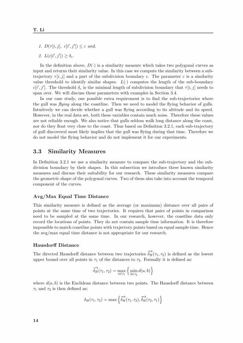
19
T. Li
is shown in Figure 3.7. We find some repeated free regions with similar shapes. Everytime the moving entity moves along the boundary, we find a separate curve in the freespace diagram. Therefore the sub-trajectories are reported separately.
Trajectory
Boundary
Figure 3.7: Free Space Diagram for Scenario 9
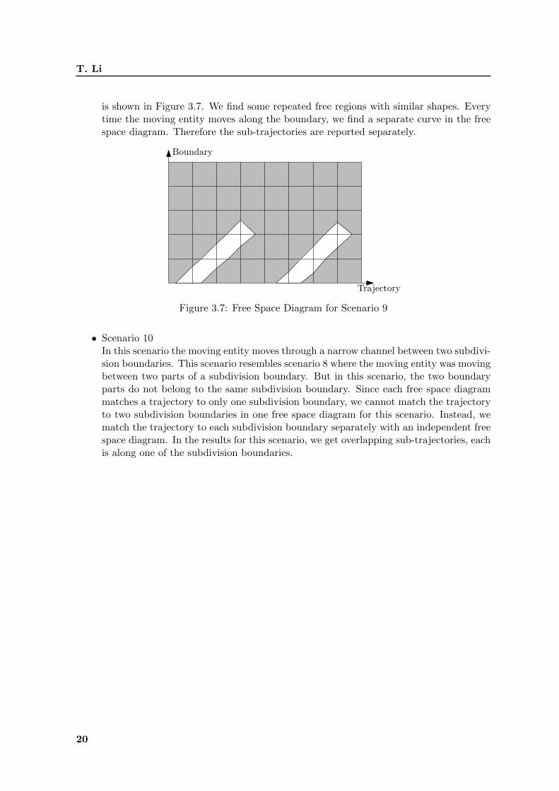
• Scenario 10In this scenario the moving entity moves through a narrow channel between two subdivi-sion boundaries. This scenario resembles scenario 8 where the moving entity was movingbetween two parts of a subdivision boundary. But in this scenario, the two boundaryparts do not belong to the same subdivision boundary. Since each free space diagrammatches a trajectory to only one subdivision boundary, we cannot match the trajectoryto two subdivision boundaries in one free space diagram for this scenario. Instead, wematch the trajectory to each subdivision boundary separately with an independent freespace diagram. In the results for this scenario, we get overlapping sub-trajectories, eachis along one of the subdivision boundaries.
20

Chapter 4
Algorithm
In this chapter we present algorithms to find sub-trajectories of the moving entity that arealong the subdivision boundaries using the Frechet distance. Our approach is based on thefree space diagram, see Section 2.2. We first introduce the main algorithm based on the weakFrechet distance in Section 4.1, then we give an algorithm to find jumps in Section 4.2. InSection 4.3 we show how to efficiently find a jump with the help of a balanced binary tree.
4.1 Main Algorithm
Our main algorithm is based on the weak Frechet distance. Alt and Godau gave an O(nm)algorithm to decide whether the weak Frechet distance between two polygonal curves is atmost ε in [1]. However, their algorithm completely matches the two curves and decides theirsimilarity value. In our research the trajectory and the subdivision boundary are partiallymatched by the weak Frechet distance. Therefore we modify the weak Frechet distancealgorithm in [1] and give our partial matching algorithm.
Given a trajectory τ with n segments and a subdivision boundary c with m segments, aswell as a parameter ε > 0, we build a free space diagram of n×m cells. The diagram is builtcolumn by column from left to right. In each column, we build the cells from bottom to top.For each cell Cij we compute Ivij , I
hij and IFij . After the free space diagram is completed, we
create an undirected graph G = (V,E) where V = {Cij | 1 ≤ i ≤ n, 1 ≤ j ≤ m}. For eachcell Cij , if Ivij 6= ∅, we add an edge connecting Cij and Ci−1j in G; If Ihij 6= ∅, we add an edgeconnecting Cij and Cij−1 in G. If Cij ∩Fε = ∅, we remove the corresponding vertex from G.
We then get a graph containing a number of disconnected components, as shown in Fig-ure 4.1. Each component represents a free space region in the free space diagram. Next wetraverse the graph with a traversal algorithm, such as breadth first search, to find all thesecomponents. During the traversal process of each component, we keep updating πc(u) andπc(u) to maintain the maximum πc(u) discovered. We then test if πc(u) ≥ δc according toDefinition 3.2.1. If so, we report the corresponding sub-trajectory.
4.2 Algorithm to Find Jumps
Recall that in Scenario 3 the moving entity moves over a gulf. Depending on the size of thegulf and the value of parameter ε we choose, we have two possible cases (See Figure 3.2).We now focus on Figure 3.2(a). By our main algorithm in Section 4.1 we will report two
21

T. Li
Figure 4.1: Free Space Diagram with Corresponding Graph
overlapping sub-trajectories τ [x, j] and τ [i, y] (i < j). However, such segmentation is notmeaningful. A more natural solution is to merge these two sub-trajectories and report τ [x, y]instead. We need a “tunnel” across the forbidden region in free space diagram to connect thetwo curves in the free space. Hence we define a jump in Definition 4.2.1.
Definition 4.2.1. Given two non-empty free space cells Cij and Cij′ with j′ < j. A jumpconnects the free space regions from Cij′ to Cij.
Trajectory
Boundary
pjpi
pi pj
qi qj
qi
qj
(a) Scenario 3 without a Jump
Trajectory
Boundary
pj
pj
qi qj
qi
qj
(b) Scenario 3 with a Jump
Figure 4.2: Example of a Jump
In Figure 4.2 we give an example jump at pj . Without the jump, the lower curve inFigure 4.2(a) is stopped at pj . The jump connects the lower curve to higher live cells sothat the curve is extended. Recall from Section 2.2 that a live cell Cij has non-empty rightboundary Ivi+1j 6= ∅. In this way we merge the two originally disconnected curves and get alonger curve in Fε.
A jump has a direction. It starts from the lower cell and ends at the upper cell. We callthe upper cell the target cell. We observe that the right boundary of target cells containsfree space, so that target cells can extend the curve discovered to the right neighbor column.By this observation we know that live cells are potential target cells to which a jump can bemade.
22

Detecting the Moving-Along Pattern in Trajectory Data
The process to find jumps can be embedded in the process to build the free space diagram.We build up the free space diagram column by column from left to right, and in each columnfrom bottom to top. Each time we encounter a live cell Cij , we search in all cells below it(from Ci0 to Cij−1) to find a cell to make a jump. Intuitively, a cell Cij′ with IFij′ ∩ IFij 6= ∅is a sufficient condition, and a jump can be made from Cij′ to Cij (j′ < j). However, we willgive examples to illustrate that this is not sufficient in the following analysis. Instead, we givethe definition of feasible jumps in Definition 4.2.2.
Definition 4.2.2. Given two non-empty cells Cij and Cij′ with j′ < j. We can make afeasible jump from Cij′ to Cij iff LFij′ ≤ LFij ≤ RFij′. We say Cij′ is a feasible cell of Cij.
5
2
10
3
Ci0 (0, 4)
Ci1 (0, 5)
Ci2 (0, 3)
Ci3 (3.5, 6)
Ci4 (0, 1)
Ci5 (2, 6)
0 6
Figure 4.3: Strategies of Jumps
According to Definition 4.2.2, for each live cell Cij , it is possible that we find more thanone feasible cell. Figure 4.3 gives an example. For each cell with non-empty left boundaryIvij 6= ∅ (Ci0, Ci1, Ci2 and Ci4), we show the length of curve in Fε discovered to its left. In the
brackets we also show parameterized LFij and RFij , by which we can compute length(IFij ). For
example, length(IFi3) = 6 − 3.5 = 2.5. We define Wij for each cell as the sum of length(IFij )and the length of curve to its left. Then we have Wi0 = 4 + 5 = 9, Wi1 = 5 + 2 = 7,Wi2 = 3 + 10 = 13, Wi3 = 2.5 + 0 = 2.5, Wi4 = 1 + 3 = 4 and Wi5 = 4 + 0 = 4. In this figure,we have two live cells: Ci5 and Ci3. For Ci3 we can make a jump from Ci0 or Ci1; for Ci5 wecan make a jump from Ci0, Ci1 or Ci2. Now the question is, which one should we choose?
Intuitively we choose the cell with maximum W value so that we can maintain the longestcurve discovered in Fε, and then report the longest sub-trajectory. With this strategy wechoose Ci2 for Ci5 and Ci0 for Ci3. However, to find the cell with maximum W , we may do alinear search downwards from the target cell. In the worst case it costs O(m) time for eachlive cell to make such a jump, where m is the number of cells in each column.
Another choice is to select the cell that is nearest to the target cell. Formally, among allthe feasible cells of Cij , we choose the cell Cij′ with minimum |j − j′|. By this strategy weminimize the length of each jump. In the example we choose Ci2 for Ci5 and Ci1 for Ci3. In
23

T. Li
Section 4.3 we show that with this strategy it costs O(logm) time to make a jump for eachlive cell. This is more efficient than the previous strategy.
Since we process the cells from bottom to top in each column of the free space diagram,we can combine these two strategies so that each live cell get the longest curve with time costO(logm). We choose the nearest feasible cell Cij′ to make the jump. However, we not onlymake jumps for live cells, but also for other cells with empty right boundary. When makingjumps we update the W value for each cell so that the optimal length of curve is propagatedupward. Thus live cells obtain the optimal W value from all feasible cells below it by makinga jump from the nearest feasible cell.
Algorithm 1 FindJumps(D, i)
1: D is the free space diagram, size n×m. i is the column index.2: for j = 0 to m− 1 do3: Find nearest feasible cell Cij′ for Cij4: UpdateLength(Cij , Cij′)5: return
Algorithm 2 UpdateLength(Cij , Cij′)
1: if Ivij = ∅ and Cij′ doesn’t exist then
2: Wij ← length(IFij )3: return4: if Ivij 6= ∅ then
5: s1 ←Wi−1j + length(IFij )6: if Cij′ exists then7: s2 ←Wij′ − length(〈LFij , RFij′〉) + length(IFij )8: Wij ← max(s1, s2)9: return
In Algorithm 2, we update Wij by taking the maximum value among Wi−1j and Wij′ .If neither of them is available, Wij is set to length(IFij ). The complexity of the algorithm isO(1).
Lemma 4.2.1. Using Algorithm 1 and 2, each live cell Cij obtains maximum Wij.
Proof. Assume we are processing a live cell Cij0 . We may have the following cases:
1. Ivij0 = ∅ and Cij0 has no feasible cells. In this case Wij0 = length(IFij0). For the cells
Cij′ below it, we have either LFij′ > LFij0 or RFij′ < LFij0 . The former type of cells have
smaller length(IFij′). For the latter type of cells, even if they may have large W values,they are not feasible for Cij0 according to Definition 4.2.2. Therefore Wij0 is optimal.See Figure 4.4(a) as an example.
2. Ivij0 = ∅ and Cij0 has feasible cells. In this case Wij0 can only be determined by itsnearest feasible cell. Assume Cij1 is the nearest feasible cell, then we have Wij0 =Wij1 − length([LFij0 , R
Fij1
]) + length(IFij0). Now if Cij1 has no feasible cells, we know
Wij0 ≥ length([LFij1 , RFij0
]). We also know that for all cells Cij′ below Cij1 , we have
24

Detecting the Moving-Along Pattern in Trajectory Data
LFij′ > LFij1 . So Wij0 is larger than any W value below Cij1 . If Cij1 has feasible cells,we iteratively compute W value of its nearest feasible cells until no feasible cells areavailable. See Figure 4.4(b) as an example.
3. Ivij0 6= ∅. In this case, the feasible cell for Cij0 can only be cells with Ivij′ 6= ∅.
If Cij0 has no feasible cells, then we know all cells below it have Ivij′ = ∅, therefore Wij′ <
length([i, j0]) for all of them. We also know that Wij0 ≤ length(IFij0) = length([i, j0]),the entire width of the column. Hence it is optimal. See Figure 4.4(c) as an example.
4. If Ivij0 6= ∅ and Cij0 has feasible cells, then Wij0 is at least length(IFij0) plus the lengthof longest curve to the left of cells below it. Assume Cij′′ has the longest curve to theleft and j′′ < j0. This implies Ivij′′ 6= ∅. Then Cij′′ can pass the length of curve upwardto all cells with Ivij′ 6= ∅ until it reaches Cij0 . Hence Wij0 is optimal. See Figure 4.4(d)as an example.
Cij0
Cij0 Cij0
Cij0
Cij′′
Cij1
Cij2
(a)
(c) (d)
(b)
Figure 4.4: Optimal Length for Live Cells
We demonstrate Algorithms 1 and 2 at the example of Figure 4.3. We start with Ci0. Itis the first cell in this column, hence Wi0 = 5 + 4 = 9. Next we process Ci1. It is possible tomake a jump from Ci0 to Ci1 and since Wi0 = 9 > 2 + 5, we make Wi1 = Wi0 − 4 + 5 = 10.Next we process Ci2. We can make a jump from Ci1 to Ci2, but the existing curve length ofCi2 is larger than Wi1, so Wi2 = 10 + 3 = 13. For Ci3, the nearest feasible cell is Ci1. Hence
25

T. Li
we make a jump from Ci1 to Ci3 and make Wi3 = 10−1.5+2.5 = 11. For Ci4 we have a jumpCi2 to Ci4 and Wi4 = 11. For Ci5, the nearest feasible cell is Ci2 according to Definition 4.2.2.We make the jump from Ci2 and set Wi5 = Wi2 = 1 + 4 = 16.
Figure 4.3 also gives an example to illustrate why IFij ∩IFij′ 6= ∅ is not a sufficient condition
to make a feasible jump. Suppose we are processing Ci5. If a cell Cij′ is feasible as long as IFij ∩IFij′ 6= ∅, then Ci3 becomes the nearest feasible cell for Ci5.Thus we update Wi5 = Wi3 = 11.However, this is not the optimal length of curve for Ci5.
Now the remaining question is how to find the nearest feasible cell efficiently (Line 3of Algorithm 1). The naive approach is to search downward from Cij until a feasible cellis discovered. This approach has complexity O(m), which results in O(m2) complexity forAlgorithm 1. Instead of the naive approach, we give an O(logm) approach with the help ofa balanced binary tree T . The approach will be introduced in Section 4.3. In short, we storethe column subdivision in a balanced binary tree and perform a query in this tree with keyLFij to find the nearest feasible cell for Cij . We then insert Cij into the tree and continue.
With the balanced binary tree T , we can change Algorithm 1 to Algorithm 3. For eachfree space cell Cij , the algorithm costs O(logm) time to find the nearest feasible cell to makethe jump, update the length and insert Cij into the balanced binary tree. Since the free spacediagram contains m×n cells, it takes O(mn logm) to find jumps for all cells in the free spacediagram.
Algorithm 3 FindJumps(D,T, i)
1: D is the free space diagram, size n ×m. T is the balance binary tree. i is the columnindex.
2: for j = 0 to m− 1 do3: sij′ ← Query(T, LFij)4: Find the corresponding cell Cij′ of line segment sij′
5: UpdateLength(Cij , Cij′)6: InsertSegment(T, sij)7: return
4.3 Find Nearest Jump with a Balanced Binary Tree
We abstract the free space interval IFij of each cell as a horizontal line segment sij in the cell.
The leftmost endpoint is at LFij and the rightmost endpoint is at RFij . We take the upperenvelope of these segments, as shown in Figure 4.5(a). For simplicity we omit the column idfor each segment and only keep the row id in the figure.
The upper envelope is shown as a dotted polyline in Figure 4.5(a). Each horizontalcomponent of the upper envelope either covers (part of) a line segment, or drops to thebottom boundary of the column. Each (part of) line segment covered is the highest in thatrange of the column confined by the corresponding horizontal component. For the horizontalcomponent that drops to the column bottom, it means that no line segment appears in thatrange.
By definition of the upper envelope, the horizontal components form a subdivision of thecolumn. We show this subdivision in Figure 4.5(a) below the free space diagram. Each partof the subdivision corresponds to a horizontal component of the upper envelope. At each
26

Detecting the Moving-Along Pattern in Trajectory Data
s0
s1
s2
s3
s4
i i+ 1
s1 s0 s2 s4 nulls2
(a) Upper Envelope and column subdivision
s2
s0
s1 nulls4
s2
(b) Binary search tree of subdivision
Figure 4.5: Column Subdivision
part of the subdivision we store the information of the (part of) line segment covered. If ahorizontal component is at the column bottom, we mark the corresponding subdivision partas “null”. Sometimes a line segment can be stored multiple times. For example the segments2 in Figure 4.5(a) is stored twice in the column subdivision. This results in that the numberof horizontal components can be larger than the number of line segments. In the followinganalysis we will see that the number of horizontal components is O(m), for a column with mrows.
Now for a new incoming cell Cij , we can do a query with value LFij in the subdivisionto find out which part contains the query value. If the result returned is “null”, we knowthat there is no feasible cell for Cij below it. If the result returned is a line segment sij′ , weknow that sij′ is the highest line segment in that range, and we return the cell Cij′ which wasrepresented by sij′ as the nearest feasible cell for Cij .
To perform such queries efficiently, we build a balanced binary tree according to the orderof the subdivision parts. In Figure 4.5(b) we give an example of the tree, which depicts thecolumn subdivision in Figure 4.5(a). With the balanced binary tree structure, our querycomplexity is O(h), where h is the height of the tree. As the tree is balanced, we haveh = logm. Therefore each cell finds the nearest feasible cell to make a jump in O(logm)time.
After we find the nearest feasible cell for Cij and make the jump, we have to insert sijinto the balanced binary tree. The newly inserted line segment sij is the highest among allexisting line segments, therefore the upper envelope is changed and the column subdivisionis affected. In Figure 4.6 we show the insertion of a line segment into the subdivision inFigure 4.5. In Figure 4.7 we show how the insertion of a new line segment affects the columnsubdivision in detail.
From Figure 4.7 we can summarize the process of inserting a new line segment sij as
27

T. Li
s0
s1
s2
s3
s4
i i+ 1
s1 nulls2
s5
s5 s4
(a) Insertion of a new line segment
s5
s1
nulls4
s2
(b) Insertion of a new line seg-ment in the balance binary tree
Figure 4.6: Column subdivision after insertion
follows: We first find the subdivision parts that contain LFij and RFij (LFij and RFij are the
endpoints of sij). For convenience we name the subdivision part that contains LFij as LN and
name the subdivision part that contains RFij as RN . In Figure 4.7 LN is labeled s1 and RNis labeled s4. Then we delete all the subdivision parts between LN and RN . After that weinsert sij between LN and RN and update the endpoints of LN and RN according to LFijand RFij .
The deletion of the subdivision parts between LN and RN costs O(m) time in the worstcase. However, as we organize the subdivision parts in a balanced binary tree, we can spendO(logm) time to perform the insertion process above, plus the time cost to maintain the treebalanced. We present the algorithms to insert a line segment into the tree in Algorithm 5.
Before introducing the insertion algorithm, we first introduce an algorithm DeleteN-odes performing efficient deletion operations, as shown in Algorithm 4. This algorithm isused in the insertion algorithm. Given a node SPLIT and a node V (V is in the subtreerooted at SPLIT ), the algorithm DeleteNodes deletes all the nodes in between themin the tree order. If V > SPLIT , then after deletion V becomes the in-order successor ofSPLIT in the tree; if V < SPLIT , then after deletion V becomes the in-order predecessorof SPLIT in the tree. Assuming V > SPLIT , the algorithm starts to search V from the
s1 nulls2s5 s4
s1 s0 s2 s4 nulls2
s5
Figure 4.7: Insertion changes the column subdivision
28

Detecting the Moving-Along Pattern in Trajectory Data
Algorithm 4 DeleteNodes(SPLIT, V )
1: SPLIT and V are both nodes in the balanced binary tree, V is in the subtree rooted atSPLIT .
2: if V < SPLIT then3: Node i← SPLIT.left-child4: while i 6= V do5: if V > i then6: i← i.right-child7: else8: Node t← i9: i← i.left-child
10: Delete t and all nodes in right sub-tree of t.11: else12: Node i← SPLIT.right-child13: while i 6= V do14: if V > i then15: Node t← i16: i← i.right-child17: Delete t and all nodes in left sub-tree of t.18: else19: i← i.left-child20: return
right child of SPLIT . Before reaching V , if the searching path turns to the right child ofa node i, then node i and its left subtree are deleted, because all these nodes are smallerthan V and larger than SPLIT ; if the searching path turns to the left child of node i, thenno deletion is performed and the searching continues. For the case that V < SPLIT , thealgorithm performs in a similar way with all criteria reversed. The time complexity of thealgorithm is O(logm).
We then introduce Algorithm 5, which inserts a line segment sij to the balanced binarytree. It starts with finding LN and RN . If LN equals RN (Line 4 of Algorithm 5), thenwe know that the two endpoints of sij fall into the same subdivision part. Then the part isdivided into two smaller pieces and the new line segment is inserted in between. Figure 4.8gives an example to illustrate this scenario. In the example s0 is divided into two parts afterthe insertion of s3. Figure 4.8 also shows how the balanced binary tree is changed. After theinsertion, the balanced binary tree may be re-balanced since it grows taller at the insertednode. From the inserted node we search upward to find the node that needs re-balancinguntil we reach the root. This process takes O(logm) time.
If LN is not equal to RN , Algorithm 5 continues to find the lowest common ancestornode of LN and RN . The lowest common ancestor node is the node where the searchingpaths from root to LN and RN begin to split. Therefore we name it the SPLIT node. Forexample, in Figure 4.5(b) the SPLIT node for s1 and s4 is the node labeled s2 at the rootof the tree. This node can be discovered in O(logm) time. Then we perform node deletionoperations with Algorithm 4. If the SPLIT node equals to LN or RN , we can performonly one-side deletion so that LN and RN become in-order neighboring in the tree afterthe deletion operations. In Figure 4.9 we show all the scenarios after deletion if LN equals
29

T. Li
Algorithm 5 InsertSegment(T, sij)
1: T is the balanced binary tree. sij is the line segment to be inserted.2: LN ← Query(T, LFij)
3: RN ← Query(T,RFij)4: if LN == RN then5: Divide LN into two nodes; Update their boundaries; Make the two nodes as left and
right child of sij .6: Insert sij to the place of LN in T .7: Re-balance the tree if necessary.8: return9: SPLIT ← FindLowestAncestor(LN,RN)
10: if SPLIT == LN then11: DeleteNodes(SPLIT,RN)12: Insert sij as right-child of LN ; Update the boundaries of LN and RN .13: Re-balance the tree if necessary.14: else if SPLIT == RN then15: DeleteNodes(SPLIT, LN)16: Insert sij as left-child of RN ; Update the boundaries of LN and RN .17: Re-balance the tree if necessary.18: else19: DeleteNodes(SPLIT, LN)20: DeleteNodes(SPLIT,RN)21: Replace SPLIT with sij ; Update the boundaries of LN and RN .22: Re-balance the tree if necessary.23: return
SPLIT ; in Figure 4.10 we show all the scenarios after deletion if RN equals SPLIT .
If LN equals SPLIT as shown in Figure 4.9, we insert sij as the right child of LN afterdeletions; if RN equals SPLIT , we insert sij as the left child of RN after deletions. After theinsertion of sij , we update the boundaries of both LN and RN according to the endpoints ofsij . Then we may need to re-balance the tree. Consider the scenario in Figure 4.9(a). The
s0 s1 s2
s3
s0 s1 s2s0s3
s1
s0 s2
s1
s3 s2
s0 s0
Figure 4.8: Insertion when LN == RN
30

Detecting the Moving-Along Pattern in Trajectory Data
LN
RN
LN
RN
(a) (b)
Figure 4.9: Scenarios after deletion, LN equals SPLIT
RN RN
(a)
LN
(b)
LN
Figure 4.10: Scenarios after deletion, RN equals SPLIT
worst case is that node RN has no subtrees but the left subtree of LN is full-grown. For suchworst case, the number of nodes that need re-balancing is O(logm). As each re-balancingoperation costs O(1) time, we need O(logm) time for re-balancing for the worst case. Henceit does not increase the time complexity of the entire insertion process.
If SPLIT 6= RN and SPLIT 6= LN (Line 18 of Algorithm 5), we need to performDeleteNodes on two sides of SPLIT . Then we find LN becomes the in-order predecessorof SPLIT and RN becomes the in-order successor of SPLIT . All possible scenarios arepresented in Figure 4.11. After deletions we replace SPLIT by sij to complete the insertion.Again, the boundaries of LN and RN are updated and the tree is re-balanced. The worstcase for re-balancing is the same as the scenario in Figure 4.9(a), thus the complexity for thisscenario is also O(logm).
According to the analysis above, each time we insert a new line segment to the column,at most 2 new nodes are inserted to the tree. Therefore the number of nodes in the tree isO(m). This is also the upper bound for the number of horizontal components of the upperenvelope in the column.
31

T. Li
SPLIT
LN RN
SPLIT
LN RN
SPLIT
RN
SPLIT
LN
LN RN
(a) (b)
(c) (d)
Figure 4.11: Scenarios after deletion, SPLIT 6= LN and SPLIT 6= RN
In summary, we use a balanced binary tree to record a subdivision of the column. Eachpart of the subdivision represents the highest free space interval of that range. Hence for eachfree space cell Cij , it takes O(logm) time to find the nearest feasible cell to make a jump.We also allow insertion into the tree in O(logm) time.
4.4 Non-monotone Jumps
The analysis above is based on the monotone Frechet distance. In Algorithm 1, we processeach column of the free space diagram from bottom to top. However, we have declared thatour research is based on the weak Frechet distance. We allow non-monotone curves in thefree space diagram. Therefore we should also allow jumps from upper cells to lower cells. Wename these jumps non-monotone jumps. In Figure 4.12 an example is presented. To find thesejumps, we need to process the free space diagram twice. In the first pass, we start from the firstcolumn (i = 0) to the last column (i = n), and at each column we call FindJumps(D,T, i)to find monotone jumps. In the second pass, we start from the last column (i = n) to thefirst column (i = 0). At each column, we still call FindJumps(D,T, i) function. However, inthis pass the Definition 4.2.2 should be slightly modified: the requirement of feasible jump is
32

Detecting the Moving-Along Pattern in Trajectory Data
changed to LFij′ ≤ RFij ≤ RFij′ , and Algorithm 2 should be modified accordingly. The secondpass can be interpreted as that we make the gull fly backwards along the trajectory and findthe jumps in free space diagram. The complexity of the two passes in total is O(mn logm).
pj
pj
qi qj
qi
qj
Trajectory
Boundary
Figure 4.12: Example of a non-monotone Jump
Once we find a jump from Cij′ to Cij , we add an edge in G connecting vertices Cij′ andCij . Thus during graph traversal, they will be regarded in the same component. Then thetwo originally disconnected components are connected. Finally, we report one sub-trajectoryfrom the component, so that the two originally overlapping sub-trajectories are merged.
33


Chapter 5
Implementation
We implemented the algorithms in Java using Eclipse. We built a GUI application to visualizethe results. We also allow exporting results to KML format files, so that they can be visualizedin Google Earth.
The entire application includes 4 types of classes, they are
• Geometry classes - including basic geometric shapes, like points, line segments, etc.
• Entity classes - including the entities, which are fixes, trajectories and subdivisionboundaries.
• Algorithm classes - including the algorithms introduced in Chapter 4.
• GUI classes - including the visualization component, the main application panel andthe KML exporting component.
The structure of the application is presented as an UML class diagram in Figure 5.2.In our initial version of the algorithm, we used an interval tree to find nearest jumps
instead of a balanced binary tree. We use this interval tree in the implementation.The capsule class in geometry classes is for determining LFij and RFij of a free space cell
Cij . For example, consider two line segments P and Q, and a parameter ε, as shown inFigure 5.1. We create a capsule-shape boundary around Q so that any point on the boundaryhas minimum distance ε to Q. The boundary encloses the Minkowski sum of the segment Qand a disk of radius ε. We then find the intersection points of P and the boundary, say piand pj . According to their positions in P we compute LFij and RFij .
ε
ε Q
P
pi
pj
Figure 5.1: Capsule Shape
35

T. Li
-Latitude : double-Longitude : double-X : double-Y : double
Point
LineSegment
Rectangle
-radius : double
Circle
Capsule
-Time : Date-Speed : double
Fix
-ID : int
Trajectory
-ID : int
Boundary
+GenerateGraph()+FindCurves()
-epsilon : double-min_coastline : double
FreeSpaceDiagram -row_id : int-col_id : int-epsilon : double-l_bound : double-r_bound : double
FreeSpaceCell
+Insert(in c : FreeSpaceCell) : void+Query(in key : double) : FreeSpaceCell
IntervalTree
KMLExporter MainPanel TrajectoryView
1 1..*
1
1
1
1
12
1
1..*
1
1
1
1..*
1
2
1
21
1
1
*
<<call>>
1
1
Geometry Classes
Entity Classes
Algorithm Classes
GUI Classes
1
1..*
Figure 5.2: Structure of the Application
36

Chapter 6
Experiments
In this chapter we evaluate the correctness of our algorithm and test it on real data. Wefirst describe experiments on synthetic data in Section 6.1 and present the results of theseexperiments in Section 6.2. Then we describe experiments with real data in Section 6.3 andshow results of these experiments in Section 6.4. All experiments were conducted on an IntelCore-2 1.73GHz PC with 2GBytes of main memory, running on Windows XP.
6.1 Experimental Setting for Synthetic Data
We first conducted experiments on synthetic data. The purpose of these experiments is toevaluate the correctness of the algorithms. We create synthetic data to simulate the scenariosdescribed in Section 3.4. We manually draw the coastline and trajectory in a java applet,and export them to comma-separated files. We test the synthetic data with the algorithmimplemented and compare the results with our expected results in Table 3.1. For the scenariothat the moving entity moves over a gulf, we test how the jumps described in Section 4.2improve the results.
Since the data sets are synthetic, the thresholds are also synthetic, and we do not attemptto obtain a uniform setting of thresholds which is suitable for all the scenarios. The purposeof these experiments is to check if the algorithms implemented can handle all the scenarioscorrectly. Therefore we adjust the setting of thresholds for each scenario to test the algorithms.
6.2 Results for Synthetic Data Experiments
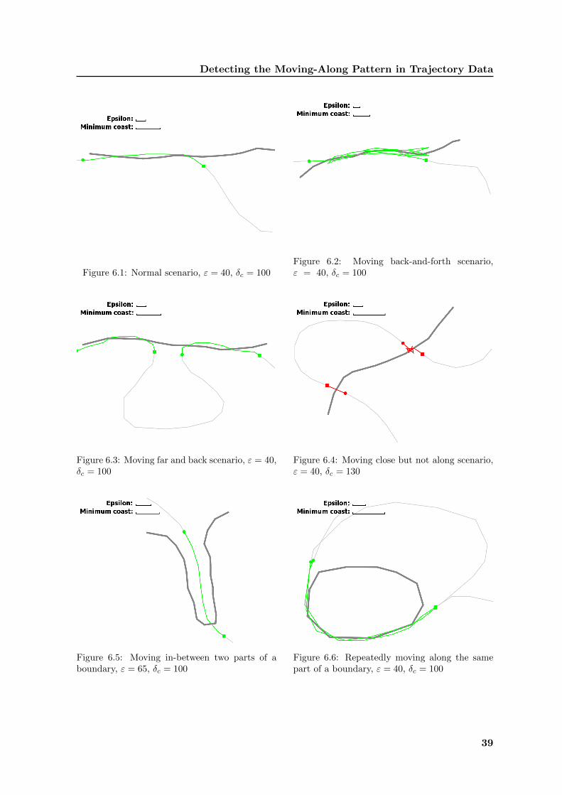
For all the figures in this section, the dark grey polylines represent the subdivision boundaryand the light grey polylines represent the trajectory. The sub-trajectories along the subdivi-sion boundary are highlighted in color green; The sub-trajectories that are close to but notalong the subdivision boundary are highlighted in color red. Each sub-trajectory has a startpoint (a filled circle) and an end point (a filled square).
Figure 6.1 shows the scenario that the moving entity moves along the subdivision bound-ary in the beginning, and then moves away from the subdivision boundary. The algorithmcorrectly finds the sub-trajectory.
Figure 6.2 shows that the moving entity moves back and forth along the subdivisionboundary. The algorithm correctly finds the sub-trajectory, which indicates that the weakFrechet distance is effective in the algorithm.
37

T. Li
Figure 6.3 shows the scenario that the moving entity moves along the subdivision boundaryinitially, then moves away for a while and finally moves along the subdivision boundary again.The algorithm correctly finds the two sub-trajectories that are along the subdivision boundary,and rules out the sub-trajectory that is far away.
Figure 6.4 shows two scenarios that the moving entity moves close to the subdivisionboundary but not along it. The algorithm correctly labels the sub-trajectories as close to thesubdivision boundary.
Figure 6.5 shows that the moving entity moves between two subdivision boundary parts.The algorithm finds the sub-trajectory and labels it as along both parts.
Figure 6.6 shows that the moving entity repeatedly moves along a part of subdivisionboundary. The algorithm correctly discovers the two sub-trajectories that are along thesubdivision boundary.
Figure 6.7 shows that the moving entity passes a gulf-shaped subdivision boundary. InFigure 6.7(a) the algorithm does not use jumps and it reports two overlapping sub-trajectories.In Figure 6.7(b) the algorithm uses jumps and only one sub-trajectory is discovered.
Figure 6.8 shows a similar scenario as the previous figure, but the moving direction of themoving entity is opposite. The algorithm correctly finds one sub-trajectory in Figure 6.8(b)with non-monotone jumps.
Figure 6.9 shows a scenario that the moving entity passes multiple gulfs. In Figure 6.9(a),four sub-trajectories are discovered without jumps and they are overlapping each other. InFigure 6.9(b), with jumps the sub-trajectories are merged.
38
Detecting the Moving-Along Pattern in Trajectory Data
Figure 6.1: Normal scenario, ε = 40, δc = 100Figure 6.2: Moving back-and-forth scenario,ε = 40, δc = 100
Figure 6.3: Moving far and back scenario, ε = 40,δc = 100
Figure 6.4: Moving close but not along scenario,ε = 40, δc = 130
Figure 6.5: Moving in-between two parts of aboundary, ε = 65, δc = 100
Figure 6.6: Repeatedly moving along the samepart of a boundary, ε = 40, δc = 100
39

T. Li
(a) without jumps (b) with jumps
Figure 6.7: Moving over a gulf, ε = 60, δc = 100
(a) without jumps (b) with jumps
Figure 6.8: Moving over a reverse gulf, ε = 40, δc = 100
(a) without jumps (b) with jumps
Figure 6.9: Moving over multiple gulfs, ε = 40, δc = 40
40

Detecting the Moving-Along Pattern in Trajectory Data
6.3 Experimental Setting for Real Data
After evaluating the correctness of the algorithms implemented in the previous section, wenow test the algorithms on real data. We first introduce the real data sets in detail, then weexplain the experiments of the real data.
Data Description
The gull data set consists of the trajectory data of 8 lesser black-backed gulls from June 1stto June 30th, 2010. Four of them are adult males and the other four are adult females. Thesize of the data ranges from around 4,000 sample points to more than 17,000 sample points.Each gull has a unique ID. In the trajectory data, each GPS record consists of the date andtime, longitude, latitude, x/y coordinates, altitude, sensor temperature, GPS speed and thedistance to the colony center. Among these variables, the altitude and GPS speed values arenot accurate; the sensor temperature and the distance to the colony center are not relevantto our research.
The sample rate of the data is not consistent. The rate depends on the energy level of thelogger attached to the gulls. It ranges from 3 seconds to 20 minutes. In Table 6.1 we give thedata information for each gull.
ID Gender Size of Data Average sample rate (minutes)
298 Male 4161 fixes 10.4
311 Male 4096 fixes 10.5
317 Male 4948 fixes 8.7
320 Male 14818 fixes 2.9
327 Female 8046 fixes 5.4
329 Female 3840 fixes 11.2
344 Female 9101 fixes 4.7
355 Female 17139 fixes 2.4
Table 6.1 Gull Data Introduction
From Table 6.1 we find that for gulls with id 298, 311, 317 and 329, the average samplerate is about 10 minutes; for gulls with id 327 and 344, the average sample rate is about 5minutes; for gulls with id 320 and 355, the average sample rate is about 2.5 minutes.
The coastline data set is obtained from National Geophysical Data Center (NGDC). Itdepicts the coastline of the northwestern part of the Netherlands mainland, as well as thecoastlines of the northwestern islands. Each sample point of the coastline is represented bylatitude and longitude. We convert them to x/y coordinates for each point.
The sample rate of the coastline data is also not consistent. For the long and straightparts of coastline, the sample rate is low. The distance between two consecutive sample pointsin these parts is about several kilometers; for the zigzag parts of coastline, such as a harbor,the sample rate increases. Here, two consecutive sample points are hundreds of meters apart.
Experiments Schedule
We perform four experiments on the real data set. In our algorithms, we have two inputparameters ε and δc. In applications, these parameters should ideally be set based on the
41

T. Li
knowledge of domain experts. However, we do not have this knowledge at hand. Thereforewe first conduct experiments to determine these parameters.
Next, we run the algorithms on all data sets to find the sub-trajectories where the gullwas moving along the coastline. We measure the following four variables:
• avgLength - the average length of the sub-trajectories in the results.
• avgSpeed - the average speed of the gull when it was moving along the coastline.
• avgDuration - the average time the gull spent to move along the coastline.
• avgCoastLength - the average length of coastline that the sub-trajectories in the resultsspan over.
First, we adjust the parameters to see how the changes of parameters influence these variables.We try to draw some ecological conclusions based on common sense. Second, we computesummary statistics for these variables and raise questions from the statistics and proposepossible explanations. It is beyond the scope of this thesis to analyze the gull behavior fromthe perspective of ecology. We leave these work to ecologists.
Our last experiment on the real data set is to find whether jumps are used and how theyimprove the results.
6.4 Results for Real Data Experiments
We start by “guessing” a range of parameter values based on common sense. We then conductexperiments and visualize the results. From the results we learn how to adjust the parametersfor more meaningful segments. We continue this process until we find a suitable parametersetting for all data sets.
The figures in this section have the same color settings as the figures in Section 6.2. Coast-lines are represented as dark grey polylines; trajectories are presented as light grey polylines.The sub-trajectories along the coastline are highlighted in green; the sub-trajectories that areclose to but not along the coastline are highlighted in red. The start point of a sub-trajectoryis represented as a filled circle and the end point is represented as a filled square. The blackpolylines represent the part of coastline that is matched to the sub-trajectory.
Determining reasonable parameter settings
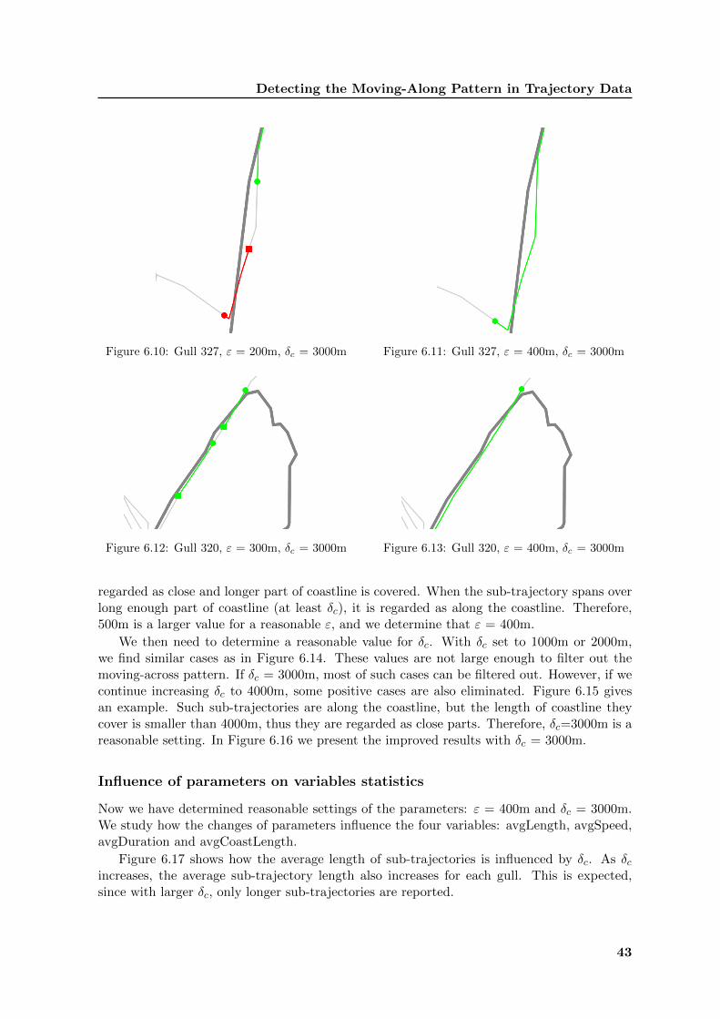
We first decide a reasonable setting of the distance parameter ε. We keep δc = 3000m in thefollowing experiments. We start with ε = 200m and find that many unnecessary segmentsare generated. Figure 6.10 provides an example. The sub-trajectory between the green partand the red part has larger distance than 200m to the coastline, therefore it is regarded asthe far-away part. However, these three parts as a whole should be regarded as along thecoastline. If we increase ε to 300m, we still find similar cases as shown in Figure 6.12.
As we increase ε to 400m, allowing a larger buffer at both sides of the coastline, we findthat many unnecessary segments are merged. Figure 6.16 and Figure 6.13 show the improvedresults for the cases mentioned above.
We continue increasing ε to 500m. Then we find that some sub-trajectories that are closeto the coastline are erroneously regarded as along the coastline. Figure 6.14 gives an example.Since we allow a 500-meter buffer at both sides of the coastline, longer sub-trajectories are
42
Detecting the Moving-Along Pattern in Trajectory Data
Figure 6.10: Gull 327, ε = 200m, δc = 3000m Figure 6.11: Gull 327, ε = 400m, δc = 3000m
Figure 6.12: Gull 320, ε = 300m, δc = 3000m Figure 6.13: Gull 320, ε = 400m, δc = 3000m
regarded as close and longer part of coastline is covered. When the sub-trajectory spans overlong enough part of coastline (at least δc), it is regarded as along the coastline. Therefore,500m is a larger value for a reasonable ε, and we determine that ε = 400m.
We then need to determine a reasonable value for δc. With δc set to 1000m or 2000m,we find similar cases as in Figure 6.14. These values are not large enough to filter out themoving-across pattern. If δc = 3000m, most of such cases can be filtered out. However, if wecontinue increasing δc to 4000m, some positive cases are also eliminated. Figure 6.15 givesan example. Such sub-trajectories are along the coastline, but the length of coastline theycover is smaller than 4000m, thus they are regarded as close parts. Therefore, δc=3000m is areasonable setting. In Figure 6.16 we present the improved results with δc = 3000m.
Influence of parameters on variables statistics
Now we have determined reasonable settings of the parameters: ε = 400m and δc = 3000m.We study how the changes of parameters influence the four variables: avgLength, avgSpeed,avgDuration and avgCoastLength.
Figure 6.17 shows how the average length of sub-trajectories is influenced by δc. As δcincreases, the average sub-trajectory length also increases for each gull. This is expected,since with larger δc, only longer sub-trajectories are reported.
43

T. Li
Figure 6.14: Gull 298, ε = 500m, δc = 3000m
Figure 6.15: Gull 327, ε = 400m, δc = 4000m Figure 6.16: Gull 327, ε = 400m, δc = 3000m
Figure 6.18 shows how the average length of sub-trajectories is influenced by ε. In generalthe average length increases with larger ε. However, for some gulls the average length dropswith larger ε. The reason for this is that new shorter sub-trajectories are included. It maybe that these gulls frequently move across the coastline. With larger ε, some sub-trajectoriesthat were close to the coastline are regarded as along the coastline. Figure 6.14 gives anexample for such case. These sub-trajectories are short and they lower the average length ofall sub-trajectories reported.
Figure 6.19 shows how the average speed is influenced by δc. With larger δc, short sub-trajectories where gulls may have been walking or floating are eliminated. Therefore weexpect that the average speed increases with larger δc. However, there is not much variancein the values. The reason may be that the values of δc we choose are quite close. No variancecan be reflected from the change of the parameter.
Figure 6.20 shows how the average speed is influenced by ε. In general the average speeddrops with increasing ε. This may be because some sub-trajectories where the gull waswalking or floating along the coastline are included.
Figure 6.21 shows how the average duration is influenced by δc. In general the aver-age duration time increases with larger δc because the average length of sub-trajectories isincreased. There is one exception with gull 329. The average duration time drops as δcincreases to 3000m. The reason may be that when δc = 2000m, a sub-trajectory where thegull was walking or floating is included. With δc = 3000m that part is eliminated, thus the
44

Detecting the Moving-Along Pattern in Trajectory Data
average duration is lowered.Figure 6.22 shows how the average duration is influenced by ε. In general the average
duration time is increased with larger ε since the average length of sub-trajectories is increased.Another explanation is that with larger ε, more walking or floating parts are included, andthey increase the average duration time.
Figure 6.23 shows how the average length of coastlines is influenced by δc. As δc increases,average length of coastline covered is also increased as expected.
Figure 6.24 shows how the average length of coastlines is influenced by ε. There is notmuch variance in the results. For some gulls the increase of average length of coastlinesis sharp, for example gull 289. The reason may be that with larger ε, two originally splitsub-trajectories are merged, so that the average length of coastline covered is increased.
Figure 6.17: Average length of sub-trajectories along the coastline, ε = 400m
Figure 6.18: Average length of sub-trajectories along the coastline, δc = 3000m
45

T. Li
Figure 6.19: Average speed of sub-trajectories along the coastline, ε = 400m
Figure 6.20: Average speed of sub-trajectories along the coastline, δc = 3000m
Figure 6.21: Average duration of sub-trajectories along the coastline, ε = 400m
46

Detecting the Moving-Along Pattern in Trajectory Data
Figure 6.22: Average duration of sub-trajectories along the coastline, δc = 3000m
Figure 6.23: Average length of coastline covered by sub-trajectories, ε = 400m
Figure 6.24: Average length of coastline covered by sub-trajectories, δc = 3000m
47

T. Li
Summary of movement statistics
Now we give a summary of movement statistics for the fixed parameters ε = 400m andδc = 3000m. The statistics are presented in Table 6.2. The average is taken over all gullswithout weighting. There is little variance in the average speed between male gulls and femalegulls. However, male gulls have larger average length of sub-trajectories. On average, theyalso spend more time than the female gulls flying along the coastline. This may be becausemale gulls more frequently make longer trips.
Variable Average for males Average for females Average for all
avgLength (m) 7648.4 5336.4 6492.4
avgSpeed (m/s) 8.0 8.3 8.1
avgDuration (min) 27.3 17.1 22.2
avgCoastLength (m) 7911.6 5543.9 6727.8
Table 6.2 Summary of statistics, ε = 400m, δc = 3000m
In Appendix A we present visualized results for each gull in Google earth. The sub-trajectories along the coastline are highlighted in green. Most gulls frequently fly along thenorthwestern coastline of the Netherlands mainland. Sometimes they fly along the coastline ofTexel island, or the coastline to the southeast of Den Helder. Gull 320 made one long journeyover the Wadden sea, and it flew along the coastlines of several islands in the northernNetherlands. Gull 317 and gull 329 had least sub-trajectories along the coastline among allthe gulls. The number of sub-trajectories along the coastline discovered for each gull is shownin Table 6.3.
Gull ID 298 311 317 320 327 329 344 355
Nr. of detected sub-trajectories 15 22 12 23 40 12 31 21
Table 6.3 Nr. of detected sub-trajectories for each gull, ε = 400m, δc = 3000m
Jumps in Real Data
We find two scenarios in which jumps are used in the real data set. We show these twoscenarios in Appendix B. In the first scenario, gull 327 frequently flew over a harbor inDen Helder. Without jumps, many overlapping sub-trajectories are regarded as close to thecoastline, because they do not span over long enough coastline parts (see Figure B.1). Withjumps, some of these overlapping sub-trajectories are merged so that they span long enoughcoastline parts as a whole. Thus they are regarded as long the coastline (see Figure B.2).
In the second scenario, gull 320 flew over the mouth of the North Sea Canal at IJmuiden.Without jumps, two overlapping sub-trajectories are detected (see Figure B.3). With jumpsthese two overlapping sub-trajectories are merged and only one sub-trajectory is reported(see Figure B.4). Note that we choose ε = 600m and δc = 2000m to illustrate this scenario.
48

Chapter 7
Conclusion
In this thesis, we have proposed a model for an entity moving along a subdivision boundary.The model uses the weak Frechet distance to compare the similarity between sub-trajectoriesof the moving entity and parts of the subdivision boundary. Based on the model we havedeveloped an algorithm to find such sub-trajectories along the boundaries. In particular, wegive an efficient algorithm to find jumps in the free space diagram, so that the sub-trajectoriesdiscovered are more meaningful.
To verify the effectiveness of our algorithm, we test them on synthetic data and realgull data. The experiments of synthetic data show the correctness of the algorithm; theexperiments of the gull data show how the results are influenced by the changes of parameters.We also interpret the results of gull data from ecological views based on common sense.
Further research on this topic includes four aspects. First, the results of experiments onthe gull data can be studied by domain experts to draw ecological conclusions. Second, themodel can be extended to include the flying behavior of gulls. Third, the model and algorithmswe presented can be applied to other scenarios like pigeons flying along roads, pedestrianswalking along streets, etc. Fourth, the algorithms can be extended to allow shortcuts in thefree space diagram to merge two close but not overlapping sub-trajectories. It may be a moremeaningful model for moving-along pattern in some applications.
49


Appendix A
Visualized Results in Google Earth
Figure A.1: Results for gull 298 on Google earth, ε = 400m, δc = 3000m
51

T. Li
Figure A.2: Results for gull 311 on Google earth, ε = 400m, δc = 3000m
Figure A.3: Results for gull 317 on Google earth, ε = 400m, δc = 3000m
52

Detecting the Moving-Along Pattern in Trajectory Data
Figure A.4: Results for gull 320 on Google earth, ε = 400m, δc = 3000m
Figure A.5: Results for gull 327 on Google earth, ε = 400m, δc = 3000m
53

T. Li
Figure A.6: Results for gull 329 on Google earth, ε = 400m, δc = 3000m
Figure A.7: Results for gull 344 on Google earth, ε = 400m, δc = 3000m
54
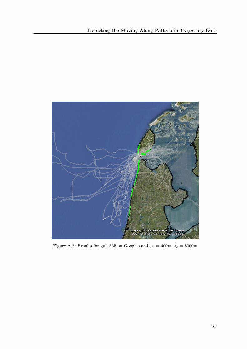
Detecting the Moving-Along Pattern in Trajectory Data
Figure A.8: Results for gull 355 on Google earth, ε = 400m, δc = 3000m
55


Appendix B
Jumps in Real Data
Figure B.1: Gull 327, without jumps Figure B.2: Gull 327, with jumps
Figure B.3: Gull 320, without jumps Figure B.4: Gull 320, with jumps
57


Bibliography
[1] Helmut Alt and Michael Godau. Computing the Frechet distance between two polygonalcurves. International Journal of Computational Geometry and Applications, 5:75–91,1995.
[2] Aris Anagnostopoulos, Michail Vlachos, Marios Hadjieleftheriou, Eamonn Keogh, andPhilip Yu. Global distance-based segmentation of trajectories. In Proceedings of the 12thACM SIGKDD international conference on Knowledge discovery and data mining, pages34 – 43, 2006.
[3] Mattias Andersson, Joachim Gudmundsson, Patrick Laube, and Thomas Wolle. Report-ing leaders and followers among trajectories of moving point objects. GeoInformatica,12(4):497 – 528, 2008.
[4] Gennady Andrienko, Natalia Andrienko, Urska Demsar, Doris Dransch, Jason Dykes,Sara Irina Fabrikant, Mikael Jern, Menno-Jan Kraak, Heidrun Schumann, and Chris-tian Tominski. Space, time and visual analytics. International Journal of GeographicalInformation Science, 24(10):1577 – 1600, 2010.
[5] David Biliotti, Gianluca Antonini, and Jean Philippe Thiran. Multi-layer hierarchicalclustering of pedestrian trajectories for automatic counting of people in video sequences.In Proceedings of the 7th IEEE Workshop on Application of Computer Vision, volume 2,pages 50 – 57, 2005.
[6] Sotiris Brakatsoulas, Dieter Pfoser, Randall Salas, and Carola Wenk. On map-matchingvehicle tracking data. In Proceedings of the 31st international conference on Very largedata bases, pages 853–864, 2005.
[7] Kevin Buchin, Maike Buchin, and Joachim Gudmundsson. Detecting single file move-ment. In Proceedings of the 16th ACM SIGSPATIAL International Conference on Ad-vances in Geographic Information Systems (ACM GIS), pages 288–297, 2008.
[8] Kevin Buchin, Maike Buchin, Joachim Gudmundsson, Maarten Loffler, and Jun Luo.Detecting commuting patterns by clustering subtrajectories. International Journal ofComputational Geometry and Applications, special issue on 19th International Sympo-sium on Algorithms and Computation (ISAAC), 21(3):253–282, 2011.
[9] Maike Buchin, Anne Driemel, Marc van Kreveld, and Vera Sacristan. Segmenting tra-jectories: A framework and algorithms using spatiotemporal criteria. Journal of SpatialInformation Science, (3):33–63, 2011.
59

T. Li
[10] Lei Chen, M. Tamer Ozsu, and Vincent Oria. Robust and fast similarity search formoving object trajectories. In Proceedings of the 2005 ACM SIGMOD internationalconference on Management of data, pages 491 – 502, 2005.
[11] Somayeh Dodge, Robert Weibel, and Anna-Katharina Lautenschutz. Towards a taxon-omy of movement patterns. Information Visualization, 7(3–4):240 – 252, 2008.
[12] Anne Driemel and Sariel Har-Peled. Jaywalking your dog: Computing the frechet dis-tance with shortcuts. In Proceedings of the 23rd Annual ACM-SIAM Symposium onDiscrete Algorithms, pages 318–337, 2012.
[13] Jason Dykes and David Mountain. Seeking structure in records of spatio-temporal be-haviour: Visualization issues, efforts and applications. Computational Statistics and DataAnalysis, 43(4):581 – 603, 2003.
[14] Zhouyu Fu, Weiming Hu, and Tieniu Tan. Similarity based vehicle trajectory clusteringand anomaly detection. In Proceedings of the IEEE International Conference on Imageprocessing, ICIP’05, volume 2, pages 602 – 605, 2005.
[15] Joachim Gudmundsson, Patrick Laube, and Thomas Wolle. Computational movementanalysis. Handbook of Geographic Information, Part C:423 – 438, 2012.
[16] Joachim Gudmundsson, Marc van Kreveld, and Bettina Speckmann. Efficient detectionof motion patterns in spatio-temporal data sets. In Proceedings of the 12th annual ACMinternational workshop on Geographic information systems, pages 250 – 257, 2004.
[17] Joachim Gudmundsson and Thomas Wolle. Towards automated football analysis: Al-gorithms and data structures. In Proceedings of the 10th Australasian Conference onMathematics and Computers in Sport, 2010.
[18] Eamonn Keogh and Michael Pazzani. Scaling up dynamic time warping for dataminingapplications. In Proceedings of the 6th ACM International Conference on KnowledgeDiscovery and Data Mining, pages 285 – 289, 2000.
[19] Eamonn Keogh and Chotirat Ann Ratanamahatana. Exact indexing of dynamic timewarping. Knowledge and Information Systems, 7:358 – 386, 2005.
[20] Jae-Gil Lee, Jiawei Han, and Kyu-Young Whang. Trajectory clustering: a partition-and-group framework. In Proceedings of the 2007 ACM SIGMOD international conferenceon Management of data (SIGMOD ’07), pages 593 – 604, 2007.
[21] Slobodan Rasetic, Jorg Sander, James Elding, and Mario Nascimento. A trajectory split-ting model for efficient spatio-temporal indexing. In Proceedings of the 31st internationalconference on Very large data bases, pages 934 – 945, 2005.
[22] Judy Shamoun-Baranes, Willem Bouten, Cornelis Jan Camphuysen, and Edwin Baaij.Riding the tide: intriguing observations of gulls resting at sea during breeding. TheInternational Journal of Avian Science, 153:411–415, 2011.
[23] Judy Shamoun-Baranes, Emiel van Loon, Ross Purves, Bettina Speckmann, DanielWeiskopf, and Cornelis Jan Camphuysen. Analysis and visualization of animal move-ment. Biology Letters, 8(1):6 – 9, 2012.
60

Detecting the Moving-Along Pattern in Trajectory Data
[24] Michail Vlachos, George Kollios, and Dimitrios Gunopulos. Discovering similar multi-dimensional trajectories. In Proceedings of the 18th International Conference on DataEngineering, pages 673 – 682, 2002.
[25] Paul Wessel and Walter Smith. A global, self-consistent, hierarchical, high-resolutionshoreline database. Journal of Geophysical Research, 101:8741 – 8743, 1996.
[26] Yutaka Yanagisawa, Jun ichi Akahani, and Tetsuji Satoh. Shape-based similarity queryfor trajectory of mobile objects. In Proceedings of the 4th International Conference onMobile Data Management, pages 63 – 77, 2003.
61