eindhoven university of technology master demand ... · in case a statistical forecasting method is...
TRANSCRIPT

Eindhoven University of Technology
MASTER
Demand forecasting through categorisation
development of a demand forecasting support model in a process industry context
Kleuskens, J.
Award date:2011
Link to publication
DisclaimerThis document contains a student thesis (bachelor's or master's), as authored by a student at Eindhoven University of Technology. Studenttheses are made available in the TU/e repository upon obtaining the required degree. The grade received is not published on the documentas presented in the repository. The required complexity or quality of research of student theses may vary by program, and the requiredminimum study period may vary in duration.
General rightsCopyright and moral rights for the publications made accessible in the public portal are retained by the authors and/or other copyright ownersand it is a condition of accessing publications that users recognise and abide by the legal requirements associated with these rights.
• Users may download and print one copy of any publication from the public portal for the purpose of private study or research. • You may not further distribute the material or use it for any profit-making activity or commercial gain
Eindhoven, September 2011
BSc Industrial Engineering and Management Science (2009)
Student identity number 0577397
in partial fulfilment of the requirements for the degree of
Master of Science
in Operations Management and Logistics
Supervisors:
dr. H.P.G. van Ooijen TU/e, Operations, Planning, Accounting and Control
dr. K.H. van Donselaar TU/e, Operations, Planning, Accounting and Control
P. Ruigt MSc. SABIC, Supply Chain Execution Polymers
M. Close MSc. SABIC, Supply Chain Execution Polymers
Demand forecasting through categorisation:
Development of a demand forecasting support model in a
process industry context
by
Jasper Kleuskens

I

II
TUE. School of Industrial Engineering.
Series Master Theses Operations Management and Logistics
Subject headings: Sales forecasting, statistical classification, supply chain management,
statistical forecasts, judgmental forecasts

III

IV
Abstract
This research project investigated the added value of statistical forecasting in a process
industry company selling commodity products. With the results obtained, a demand
forecasting support model has been developed that gives insights when to forecast
demand statistically or judgmentally for short-term tactical planning. Despite the
significant classification performance, applying the support model did not lead to an
improved forecasting performance. The main contribution of this research is the insights
it generated when judgmental forecasting is preferred over statistical forecasting.

V
VI
Management summary
SABIC Europe Polymers (SABIC EUP) initiated this research, with the objective to get
more insights in the contingent variables of demand forecasting. With the relatively long
replenishment lead times (1- 3 months) and the relatively short customer lead times (1
day – 3 weeks), demand must be supplied from stock. To enable the timely supply of
demand from stock, forecasting plays a crucial role.
In a make to stock environment, the objective of demand forecasting is to develop the
most accurate forecasts possible, specifying the expected demand for each SKU at each
of the stock points (SKU+warehouse). For the grades produced in Europe, only one
warehouse is in use. The grades imported from KSA are stored in seven warehouses
across Europe, which increases the forecasting complexity.
The analysis of the current demand forecasting procedure showed that currently no
formal methods are in place to structure the demand forecasting procedure, increasing the
complexity of developing accurate demand forecasts. As a result, the forecast error are
higher, resulting in higher costs in the supply chain (e.g. production, inventory and
opportunity costs). To provide more insights in the contingent variables of demand
forecasting, a demand forecasting support model is developed that can be used to
determine how specific demand series need to be forecasted.
Determining best demand forecasting procedure to develop forecasts The objective of demand forecasting is to develop forecasts that minimise the forecast
error on SKU+warehouse level, as this is the Customer Order Decoupling Point (CODP).
The conclusions of this research project was that that this objective is realised forecasting
demand at the same level by applying both statistical and judgmental forecasting
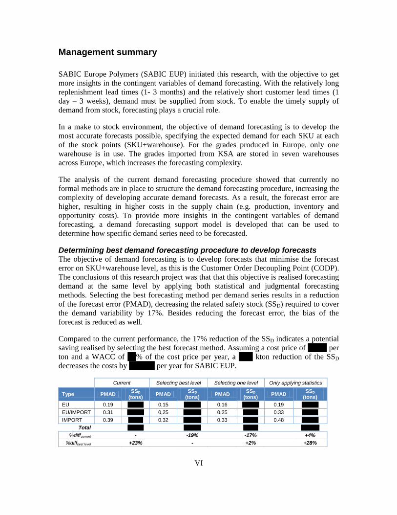
methods. Selecting the best forecasting method per demand series results in a reduction
of the forecast error (PMAD), decreasing the related safety stock (SSD) required to cover
the demand variability by 17%. Besides reducing the forecast error, the bias of the
forecast is reduced as well.
Compared to the current performance, the 17% reduction of the SSD indicates a potential
saving realised by selecting the best forecast method. Assuming a cost price of '''''' '''''' per
ton and a WACC of ''''''% of the cost price per year, a '''''''''' kton reduction of the SSD
decreases the costs by '''''''''''' ''''' per year for SABIC EUP.
Current Selecting best level Selecting one level Only applying statistics
Type PMAD SSD
(tons) PMAD
SSD
(tons) PMAD
SSD
(tons) PMAD
SSD
(tons)
EU 0.19 '''''''''''''''' 0,15 ''''''''''''''''' 0.16 ''''''''''''''''' 0.19 '''''''''''''''''
EU/IMPORT 0.31 ''''''''''''''''' 0,25 '''''''''''''''''' 0.25 ''''''''''''''' 0.33 ''''''''''''''''
IMPORT 0.39 ''''''''''''''' 0,32 '''''''''''''''''' 0.33 ''''''''''''''' 0.48 '''''''''''''''''
Total
'''''''''''''
''''''''''''''
''''''''''''
'''''''''''''''
%diffcurrent -
-19%
-17%
+4%
%diffbest level +23%
-
+2%
+28%
VII
Other scenarios were considered as well. Selecting the best forecast level per grade
resulted in an additional reduction of the PMAD, decreasing the SSD further by 2%. As
this solution requires multiple forecast level, the small decrease of SSD is not considered
an improvement, as the complexity of the procedure increases. This increase in
complexity is not preferred as it will increase costs and time to develop the forecasts.
Another scenario was to consider only statistical forecasting methods, resulting in an
overall increase of the PMAD and SSD of 4% compared to the current situation.
In practice, the proposed solution is difficult to realise, as it is not possible to determine
upfront if either statistical or judgmental forecasting methods are required to forecast
demand. To solve this problem, a demand forecasting support model is developed by
answering the second research question.
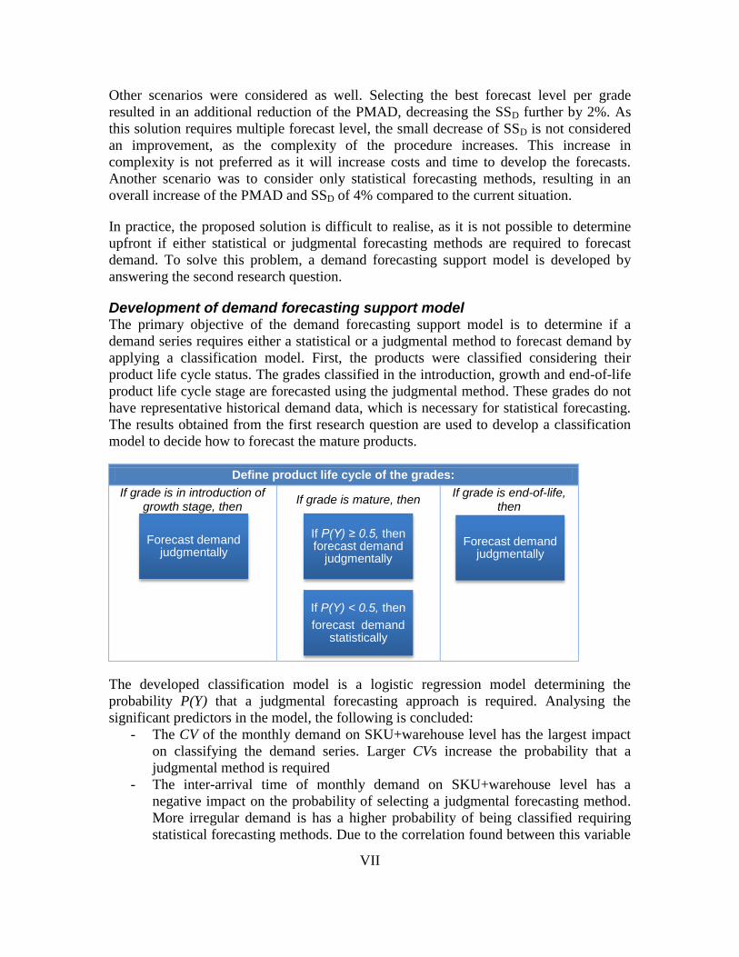
Development of demand forecasting support model The primary objective of the demand forecasting support model is to determine if a
demand series requires either a statistical or a judgmental method to forecast demand by
applying a classification model. First, the products were classified considering their
product life cycle status. The grades classified in the introduction, growth and end-of-life
product life cycle stage are forecasted using the judgmental method. These grades do not
have representative historical demand data, which is necessary for statistical forecasting.
The results obtained from the first research question are used to develop a classification
model to decide how to forecast the mature products.
Define product life cycle of the grades:
If grade is in introduction of growth stage, then
If grade is mature, then If grade is end-of-life,
then
The developed classification model is a logistic regression model determining the
probability P(Y) that a judgmental forecasting approach is required. Analysing the
significant predictors in the model, the following is concluded:
- The CV of the monthly demand on SKU+warehouse level has the largest impact
on classifying the demand series. Larger CVs increase the probability that a
judgmental method is required
- The inter-arrival time of monthly demand on SKU+warehouse level has a
negative impact on the probability of selecting a judgmental forecasting method.
More irregular demand is has a higher probability of being classified requiring
statistical forecasting methods. Due to the correlation found between this variable
Forecast demand judgmentally
If P(Y) ≥ 0.5, then forecast demand
judgmentally
If P(Y) < 0.5, then
forecast demand statistically
Forecast demand judgmentally
VIII
and the previous variable, this result should be interpreted with caution and more
research is required to validate this results.
- Both the average monthly demand at SKU+warehouse level and the average
monthly order size at SKU+ship-to level are also included in the classification
model. However, these variables have limited practical relevance, as their impact
is very small.
This research project also investigated the possibility to categorise the statistical
forecasting methods. However, due to the violations of critical assumptions of the
method, no classification model could be developed.
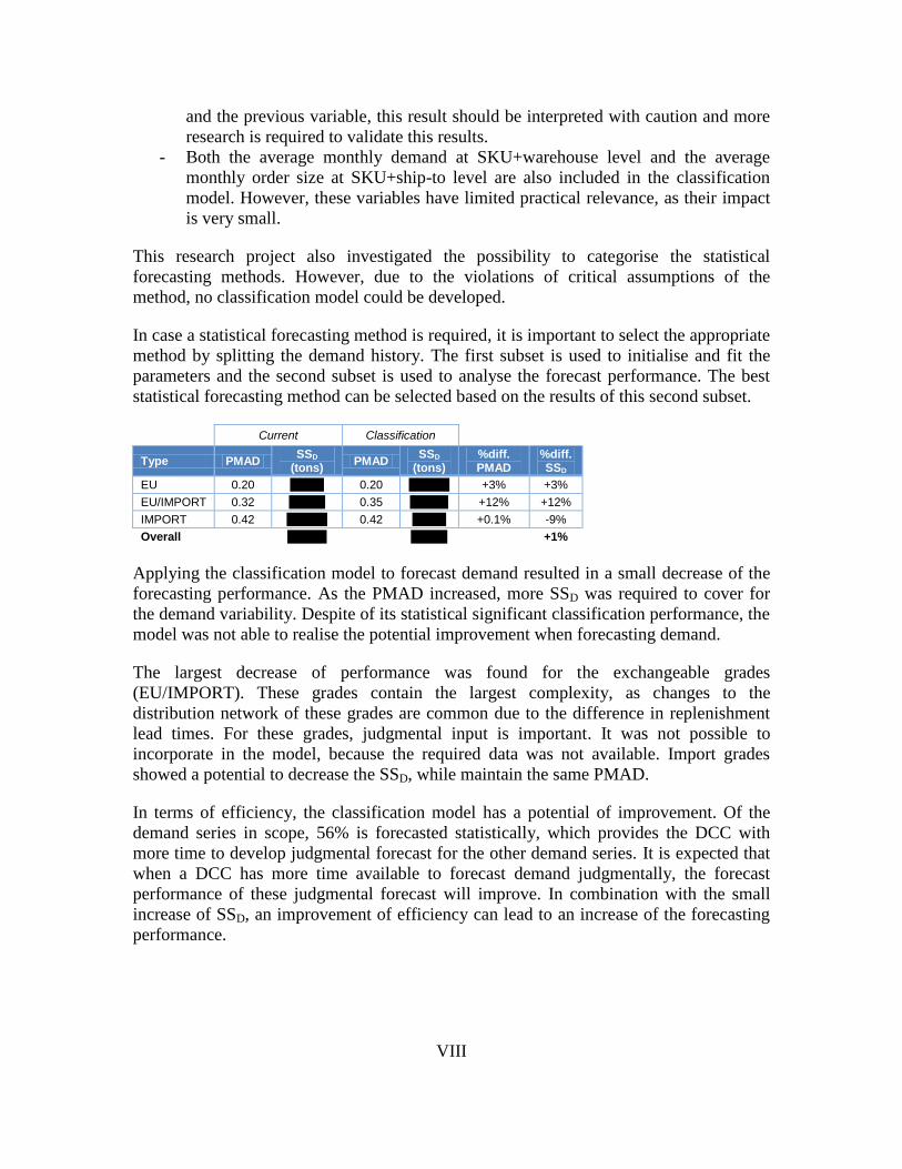
In case a statistical forecasting method is required, it is important to select the appropriate
method by splitting the demand history. The first subset is used to initialise and fit the
parameters and the second subset is used to analyse the forecast performance. The best
statistical forecasting method can be selected based on the results of this second subset.
Current Classification
Type PMAD SSD
(tons) PMAD
SSD (tons)
%diff. PMAD
%diff. SSD
EU 0.20 ''''''''''''''' 0.20 '''''''''''''''''' +3% +3%
EU/IMPORT 0.32 '''''''''''''''' 0.35 ''''''''''''''''' +12% +12%
IMPORT 0.42 '''''''''''''''''' 0.42 ''''''''''''''' +0.1% -9%
Overall
''''''''''''''
'''''''''''''
+1%
Applying the classification model to forecast demand resulted in a small decrease of the
forecasting performance. As the PMAD increased, more SSD was required to cover for
the demand variability. Despite of its statistical significant classification performance, the
model was not able to realise the potential improvement when forecasting demand.
The largest decrease of performance was found for the exchangeable grades
(EU/IMPORT). These grades contain the largest complexity, as changes to the
distribution network of these grades are common due to the difference in replenishment
lead times. For these grades, judgmental input is important. It was not possible to
incorporate in the model, because the required data was not available. Import grades
showed a potential to decrease the SSD, while maintain the same PMAD.
In terms of efficiency, the classification model has a potential of improvement. Of the
demand series in scope, 56% is forecasted statistically, which provides the DCC with
more time to develop judgmental forecast for the other demand series. It is expected that
when a DCC has more time available to forecast demand judgmentally, the forecast
performance of these judgmental forecast will improve. In combination with the small
increase of SSD, an improvement of efficiency can lead to an increase of the forecasting
performance.
IX
Different reasons have been addressed that could explain the large deviation between the
potential improvement and actual performance. A summary is presented in the next
section as recommendation to SABIC EUP. These issues need to be addressed before
continuing with the model, because it is assumed to have a significant impact on the
performance.
Recommendations to SABIC EUP - Save both the initial forecast before S&OP and the agreed forecast after S&OP to
give better representation of the expected demand. Especially when the initial
forecast has been adjusted based on information available during S&OP. The
reasons for adjustments contain valuable information and insights for demand
forecasting.
- Record lost sales and extreme events to develop a better representation of actual
demand. This information is essential for demand forecasting, because the bias
between actual demand and sales is minimised.
- Record changes in the distribution network. This is important, because it results in
a more accurate representation of demand, especially as demand forecasts are
developed at SKU+warehouse level.
- Conduct a pilot, parallel to the current procedure, to get a complete overview of
the impact on the supply chain of SABIC EUP. Bottlenecks of the new support
model can be identified and can be solved accordingly.
- Measure both the forecast error and bias to determine the forecasting
performance. Monitoring the performance and providing feedback to the planners
is essential to control the demand forecasting performance and to create an
environment of continuous improvement.
- Investigate how the demand forecasting support model can be integrated into SAP
APO, using the available functionality of this SAP module.
For future research at SABIC EUP, the following areas are proposed:
- Differentiate the demand forecasting procedure for different planning horizons.
Besides the developed solution for short-term tactical planning, other planning
horizons are present. For SABIC EUP, it is important to define the differences
between these horizons in terms of its objectives and to design a forecasting
procedure that fits these objectives.
- Investigate how distribution capacity forecasting can be differentiated from
demand forecasting, as the current research project is focused on demand
forecasting only. The current practice is to provide distribution capacity planning
with demand forecast data. The recommendations of this research will result in a
small reduction of the information accuracy required for distribution capacity
planning. To improve the distribution capacity forecasting, differentiation is
proposed.

X
Preface
This report is the results of a Master thesis project, which I conducted in partial fulfilment
for the degree of Master of Science in Operations Management and Logistics at
Eindhoven University of Technology. This project was conducted in cooperation with
SABIC, located in Sittard.
From SABIC, I would like to thank both Paul Ruigt and Marc Close, who initiated this
project and gave me the opportunity to conduct my graduation project in such a dynamic
and challenging environment as SABIC. You both fully supported me along the way and
invested a lot of time in this project to discuss the findings and to challenge me. Finally, I
want to thank everyone else at SABIC that made time for me to provide me with
information and answer my questions.
From the university, I would like to thank Henny van Ooijen, my primary supervisor, for
his enthusiasm and support during the project. Our discussions were very helpful for the
progress of my project. As my second supervisor, I would like to thank Karel van
Donselaar for his time and critical reviews of my work.
As this project ends my life as a student, I would like to thank my family and friends for
their support. Without you I would not be at the point where I am now. Special thanks go
to my mother, who raised me as the person I am today. Finally, I would like to thank
Anouk for her unconditional love, support and patience. Thank you so much.
Jasper Kleuskens
Eindhoven, September 2011

XI
XII
Table of Contents
ABSTRACT ........................................................................................................ IV
MANAGEMENT SUMMARY .............................................................................. VI
PREFACE ............................................................................................................ X
1. BACKGROUND INFORMATION .................................................................. 1
1.1. SABIC ................................................................................................................................................ 1
1.1.1. SABIC Europe Polymers ............................................................................................................... 1
1.1.2. Products....................................................................................................................................... 2
1.2. Supply chain description .................................................................................................................. 3
1.2.1. European supply chain ................................................................................................................ 3
1.2.2. Import supply chain ..................................................................................................................... 4
1.3. Supply chain planning ...................................................................................................................... 5
1.3.1. Sales & Operations Planning ....................................................................................................... 6
1.3.2. Demand planning ........................................................................................................................ 7
1.4. Supply chain challenges ................................................................................................................... 8
2. PROBLEM DEFINITION AND RESEARCH APPROACH ............................ 9
2.1. Demand forecasting challenges ....................................................................................................... 9
2.1.1. Demand forecasting differentiation ............................................................................................ 9
2.1.2. Method of demand forecasting................................................................................................. 10
2.1.3. Level of forecasting ................................................................................................................... 10
2.1.4. Access to business information ................................................................................................. 11
2.1.5. Organisational and managerial issues ....................................................................................... 11
2.2. Problem statement ........................................................................................................................ 12
2.3. Literature review ............................................................................................................................ 12
XIII
2.3.1. Demand forecasting framework ................................................................................................ 12
2.4. Research assignment ..................................................................................................................... 14
2.5. Project scope .................................................................................................................................. 15
2.6. Research methodology .................................................................................................................. 16
3. ANALYSIS OF CURRENT SITUATION ...................................................... 17
3.1. Demand characteristics .................................................................................................................. 17
3.2. Forecast accuracy ........................................................................................................................... 20
3.3. Forecast bias .................................................................................................................................. 21
4. METHODOLOGY TO DETERMINE BEST DEMAND FORECASTS .......... 23
4.1. Demand forecasting objective ....................................................................................................... 23
4.2. Forecasting methods ...................................................................................................................... 24
4.3. Levels of forecasting ....................................................................................................................... 25
4.4. Disaggregation method .................................................................................................................. 25
4.5. Performance measurement ........................................................................................................... 26
4.6. Methodology .................................................................................................................................. 28
5. RESULTS OF DETERMINING BEST DEMAND FORECASTS .................. 30
5.1. Scenario 1: determine best forecast level per grade ..................................................................... 30
5.2. Scenario 2: determine one forecast level for all grades................................................................. 31
5.3. Scenario 3: only considering statistical forecasting methods ........................................................ 32
5.4. Overall performance ...................................................................................................................... 33
5.4.1. Forecast error ............................................................................................................................ 33
5.4.2. Forecast bias .............................................................................................................................. 34
5.4.3. Forecasting methods ................................................................................................................. 35
6. DEVELOPMENT OF DEMAND FORECASTING SUPPORT MODEL ........ 36
6.1. Suggested classification variables .................................................................................................. 36
XIV
6.2. Statistical versus judgmental forecasting ....................................................................................... 38
6.2.1. Method of analysis .................................................................................................................... 38
6.2.2. Discussing results logistic regression model ............................................................................. 39
6.2.3. Determining classification performance ................................................................................... 42
6.3. Classifying statistical forecasting methods .................................................................................... 43
6.4. Summary of demand forecasting support model .......................................................................... 45
6.4.1. Evaluation of solution ................................................................................................................ 47
7. IMPLEMENTATION .................................................................................... 48
7.1. Demand forecasting procedure using the support model ............................................................. 48
8. CONCLUSION AND RECOMMENDATIONS .............................................. 50
8.1. Conclusions .................................................................................................................................... 50
8.2. Recommendations to SABIC EUP ................................................................................................... 51
8.3. Recommendations for future research .......................................................................................... 53
REFERENCES ................................................................................................... 54
GLOSSARY OF TERMS .................................................................................... 56
APPENDIX A ...................................................................................................... 57
APPENDIX B ...................................................................................................... 61
APPENDIX C ...................................................................................................... 66
APPENDIX D ...................................................................................................... 71
APPENDIX E ...................................................................................................... 75
APPENDIX F ...................................................................................................... 80

XV
1
1. Background information
SABIC initiated this research project with the objective to understand demand planning
better and to get more insights in its contingent variables. Demand planning is an
important element of supply chain management. The objective of supply chain
management is to integrate the demand and supply processes within a company by
structuring the internal processes enabling the supply of customer demand in the future
(Jüttner et al., 2007).
This chapter presents relevant background information with regard to this research
project. Section 1.1 introduces SABIC to the reader by providing a general description of
the company. This research project is conducted at the Strategic Business Unit (SBU)
Polymers of SABIC. More information of this SBU is presented in Section 1.1.1 and the
products sold are discussed in Section 1.1.2. The supply chain structure is an important
determinant in demand planning and an overview is presented in Section 1.2, where
supply chain planning is discussed in Section 1.3. Finally, the challenges of SABIC are
summarised in Section 1.4.
1.1. SABIC
The Saudi Basic Industries Corporation (SABIC) is one of the top 10 petrochemical
companies in the world, employing 33,000 people worldwide, with operations in more
than 40 countries and around 60 world-class manufacturing and compounding complexes
across the Middle East, Asia, Europe and the Americas. SABIC is composed of six
Strategic Business Units (SBUs): Chemicals, Innovative Plastics, Performance
Chemicals, Polymers, Fertilizers and Metals. The generated sales revenue over 2010 was
US$ 39.8 billion with a net income of US$ 5.5 billion. SABIC produced 66.8 million
metric tons, where Chemicals represented 63%, Polymers 16%, Fertilizers 11%, Metals
8%, Innovative Plastics 2% and Performance Chemicals 1%.
In 1976, SABIC was founded in the Kingdom of Saudi Arabia (KSA), by transforming
natural gas, a useless by-product of oil exploration, into valuable petrochemical products
that could be sold. At this moment, SABIC is one of the fastest-growing global
petrochemical companies and has the vision to be the preferred world leader in chemicals
in 2020. To achieve this, SABICs mission is to provide quality products and services
through innovation, learning and operational excellence while sustaining maximum value
for their stakeholders responsibly.
1.1.1. SABIC Europe Polymers In Europe, SABIC is a major producer of plastics, chemicals and innovative plastics and
employs around 6,000 people. The European main office of the SBUs Polymers and
Chemicals is based in Sittard (The Netherlands), whereas the main office of the SBU
Innovative Plastics is located in Bergen op Zoom (The Netherlands).
2
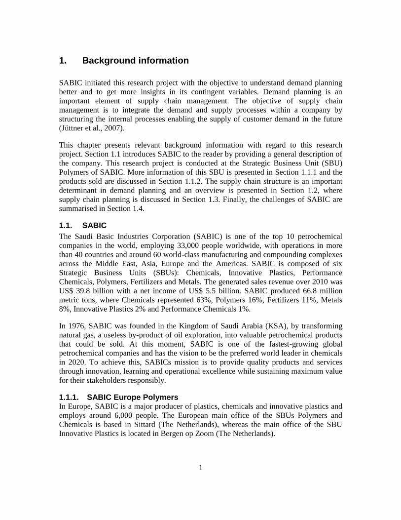
The SBU Polymers consists of different Business Units (BUs), where each BU represents
a product group hdPE, ld/lldPE and Moulding & Extrusion (PP), respectively. Each BU
consists of different Value Teams (VTs), where each VT is a group of grades that serve a
specific business. For an overview of these BUs and their related VTs, see Figure 1.1.
SBU Europe
Polymers
(SABIC EUP)
BU
ld/lldPE
BU
Moulding &
Extrusion (PP)
BU
hdPE
BU
Automotive (PP)
Technology
Management
Supply Chain
Execution
Supply Chain
Planning
Customer
Service
Supply Chain
Sourcing &
Contracting
Supply Chain
Improvements
VT
hdPE BM & Film
VT
hdPE Pipe
VT
hdPE IM
VT
3P
VT
ldPE Autoclave
VT
ldPE Tubular
VT
lldPE
VT
PP Copol
VT
Hopol
VT
PP Random
Warehouse
Operations
Figure 1.1 Organisation SBU Polymers
This project is conducted at the Supply Chain Planning department, which is a sub-
department of the Supply Chain Execution department of SABIC EUP. The main
responsibility of the Supply Chain Planning department is to manage the demand and
supply processes within the SBU Polymers in Europe.
This project was conducted at SABIC Europe Polymers, from this point forward referred
to as SABIC EUP. In the upcoming sections, some background information is given with
regard to the products sold and a general supply chain description is presented. This
chapter is concluded discussing the supply chain challenges.
1.1.2. Products SABIC EUP sells two of the most important polymers, which are used by a large group
of downstream manufacturers. These polymers are:
- Polyethylene (PE); subdivided in high density PE (hdPE), low density PE (ldPE)
and linear low density PE (lldPE). These products are supplied to extrusion, blow
moulding, injection moulding and extrusion coating businesses. Their main
applications are in flexible packaging, like film, food packaging, carrier bags and
photo-coatings, and rigid packaging, like bottles, cans, crates and boxes.
- Polypropylene (PP); has a wide range of applications and is used by injection
moulding and extrusion businesses to produce flexible and rigid packaging, fibres,
caps & closures, automotive parts and pipes.
3
At SABIC EUP, the products are subdivided into grades, where a grade is characterised
by a set of unique and identical (chemical) properties. These properties concern e.g. the
melt index, density and colour of the product and each grade is characterised by a unique
code. Some grades are exchangeable with each other, meaning that customers can be
supplied with multiple grades. As will be discussed later, these grades are considered as
one for demand forecasting purposes.
The production processes produce granulates of a specific grade. These granulates are
stored directly in a silo. If necessary, the stored grades can be packed and stored in a
warehouse. These stored grades are the so-called Stock Keeping Units (SKUs). At
SABIC EUP, four types of packaging modes are present; bulk, big-bags, bags and
octabins. Bulk and bags are the most common used packaging modes.
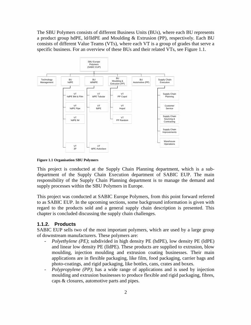
1.2. Supply chain description
The supply chain network of SABIC EUP consists of multiple production facilities and
hubs for import across Europe, as visualised in Figure 1.2. The sales are managed
through an extensive network of local sales offices throughout Europe.
The supply chain of SABIC EUP is divided for the grades produced in Europe and grades
imported from SABIC KSA. There are some exceptions, where grades are supplied by
both Europe and KSA. The supply of these grades is managed by certain costs rules. In
the next section, both supply chains are presented to give a general overview. These
grades are defined as exchangeable grades.
Figure 1.2 Supply chain network of SABIC EUP
1.2.1. European supply chain The European supply chain consists of four polymer production sites, located in Geleen
(The Netherlands), Gelsenkirchen (Germany) Wilton (UK) and Genk (Belgium). Each of
these production facilities produces a certain group of grades. In general, grades are
4
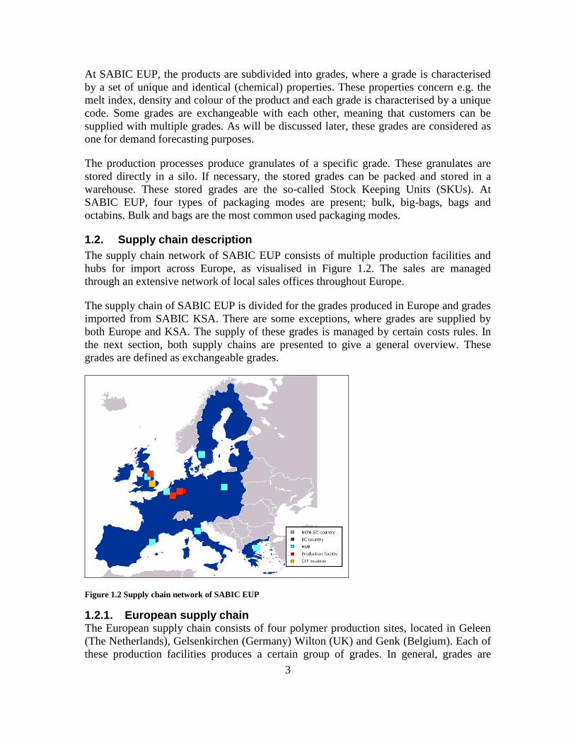
produced at one manufacturing facility only, except for a couple of exchangeable grades.
Products produced in Europe are referred to as EU grades. A general overview of the
European supply chain is presented in Figure 1.3.
Figure 1.3 Supply chain of European grades of SABIC EUP
After production, the grade is stored in silos or packed. In case the grade is packed, it is
stored in warehouses around the production site. For some customers the option exists to
store bulk containers closer to the customer to shorten the lead time. These locations are
defined as Container-In-Transit (CIT) locations. Currently, two CIT locations are in use
in the UK and one in Finland. These CIT locations are exceptional and therefore
excluded from this research.
Customers are supplied from the stocks located in warehouses and silos, with a lead time
equal to the transportation time (customer lead time). At these stock points, the grades are
replenished based on a make-to-stock strategy and a given lead time (replenishment lead
time). As a result, it is concluded that the Customer Order Decoupling Point (CODP) is
positioned at these stock points. The CODP defines the penetration point of a customer
order into the supply chain (De Kok and Fransoo, 2003).
At SABIC EUP, production takes place continuously by applying a production cycle.
This cycle is an optimised sequence of the grades produced, by minimising the transition
time and material. The length of this production cycle varies between 0.5 to 1 month,
depending on the production facility.
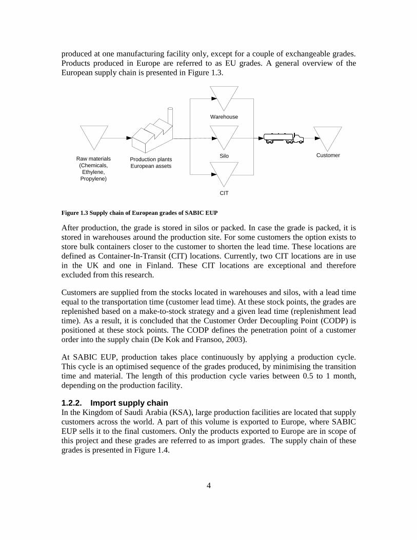
1.2.2. Import supply chain In the Kingdom of Saudi Arabia (KSA), large production facilities are located that supply
customers across the world. A part of this volume is exported to Europe, where SABIC
EUP sells it to the final customers. Only the products exported to Europe are in scope of
this project and these grades are referred to as import grades. The supply chain of these
grades is presented in Figure 1.4.
Raw materials
(Chemicals,
Ethylene,
Propylene)
CIT
Silo
Warehouse
CustomerProduction plants
European assets

5
Figure 1.4 Supply chain of imported grades of SABIC EUP
After production in KSA, the grades are transported over sea to different warehouses
(hubs) in Europe. These warehouses are used for import materials and are located in
Bologna (Italy), Wallhamn (Sweden), Tarragona (Spain), Kallo (Belgium), Kutno
(Poland), Thessaloniki (Greece) and Middlesbrough (UK). This year, a new warehouse
will be introduced in Sittard (The Netherlands) to manage the expected growth of
imported grades. Customers are linked to a specific warehouse from which they are
supplied. The allocation of a customer to a specific warehouse is obtained through the
Supply Network Planning (SNP) model. In this model, the allocation of a customer to a
warehouse is determined by minimising the transportation costs. This year, it has been
decided to start supplying EU grades from these warehouses as well. Due to the recent
introduction and very small volumes, this option is out of scope for this research.
As for EU grades, the CODP for imported grades is positioned at the warehouses from
which customers are supplied. The customer lead time of imported grades equals the
transportation time from the warehouse to the customer. The replenishment lead time
depends on the production cycle applied in KSA and the transportation time required to
ship the materials to the different warehouses around Europe. Due to these transportation
times, the replenishment lead time is between 2 to 3 months, which is quite large
compared to the EU grades.
The relative long replenishment lead time of these products and the relative short
customer lead time, make demand planning a crucial step in supply chain planning. In the
upcoming sections, supply chain planning at SABIC EUP is presented to give more
relevant background information and to discuss the role of demand planning in a supply
chain.
1.3. Supply chain planning
The main objective of supply chain planning is to balance supply with demand, taking
into considerations different planning horizons. At SABIC EUP, different horizons are
applied see Table 1.1. On strategic level, yearly sales budgets are created by Business
Raw materials
(Chemicals,
Ethylene,
Propylene)
Warehouse
at KSA plant
Transportation
over sea to
Europe
Warehouse 1
Warehouse 2
Warehouse 7
Customer
Production plants
KSA
Customer
Customer
Transportation
over sea to
other parts of
the world
(out of scope)
6
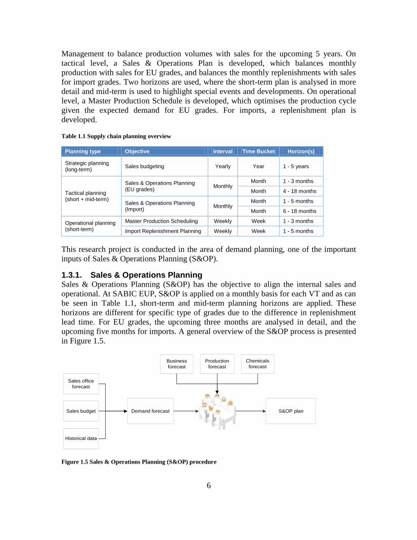
Management to balance production volumes with sales for the upcoming 5 years. On
tactical level, a Sales & Operations Plan is developed, which balances monthly
production with sales for EU grades, and balances the monthly replenishments with sales
for import grades. Two horizons are used, where the short-term plan is analysed in more
detail and mid-term is used to highlight special events and developments. On operational
level, a Master Production Schedule is developed, which optimises the production cycle
given the expected demand for EU grades. For imports, a replenishment plan is
developed.
Table 1.1 Supply chain planning overview
Planning type Objective Interval Time Bucket Horizon(s)
Strategic planning (long-term)
Sales budgeting Yearly Year 1 - 5 years
Tactical planning (short + mid-term)
Sales & Operations Planning (EU grades)
Monthly Month 1 - 3 months
Month 4 - 18 months
Sales & Operations Planning (Import)
Monthly Month 1 - 5 months
Month 6 - 18 months
Operational planning (short-term)
Master Production Scheduling Weekly Week 1 - 3 months
Import Replenishment Planning Weekly Week 1 - 5 months
This research project is conducted in the area of demand planning, one of the important
inputs of Sales & Operations Planning (S&OP).
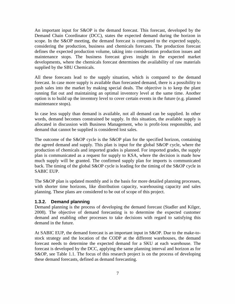
1.3.1. Sales & Operations Planning Sales & Operations Planning (S&OP) has the objective to align the internal sales and
operational. At SABIC EUP, S&OP is applied on a monthly basis for each VT and as can
be seen in Table 1.1, short-term and mid-term planning horizons are applied. These
horizons are different for specific type of grades due to the difference in replenishment
lead time. For EU grades, the upcoming three months are analysed in detail, and the
upcoming five months for imports. A general overview of the S&OP process is presented
in Figure 1.5.
Figure 1.5 Sales & Operations Planning (S&OP) procedure
Sales office
forecast
Sales budget
Historical data
Demand forecast
Business
forecast
Production
forecast
Chemicals
forecast
S&OP plan
7
An important input for S&OP is the demand forecast. This forecast, developed by the
Demand Chain Coordinator (DCC), states the expected demand during the horizon in
scope. In the S&OP meeting, the demand forecast is compared to the expected supply,
considering the production, business and chemicals forecasts. The production forecast
defines the expected production volume, taking into consideration production issues and
maintenance stops. The business forecast gives insight in the expected market
developments, where the chemicals forecast determines the availability of raw materials
supplied by the SBU Chemicals.
All these forecasts lead to the supply situation, which is compared to the demand
forecast. In case more supply is available than forecasted demand, there is a possibility to
push sales into the market by making special deals. The objective is to keep the plant
running flat out and maintaining an optimal inventory level at the same time. Another
option is to build up the inventory level to cover certain events in the future (e.g. planned
maintenance stops).
In case less supply than demand is available, not all demand can be supplied. In other
words, demand becomes constrained be supply. In this situation, the available supply is
allocated in discussion with Business Management, who is profit-loss responsible, and
demand that cannot be supplied is considered lost sales.
The outcome of the S&OP cycle is the S&OP plan for the specified horizon, containing
the agreed demand and supply. This plan is input for the global S&OP cycle, where the
production of chemicals and imported grades is planned. For imported grades, the supply
plan is communicated as a request for supply to KSA, where the decision is made how
much supply will be granted. The confirmed supply plan for imports is communicated
back. The timing of the global S&OP cycle is leading for the timing of the S&OP cycle in
SABIC EUP.
The S&OP plan is updated monthly and is the basis for more detailed planning processes,
with shorter time horizons, like distribution capacity, warehousing capacity and sales
planning. These plans are considered to be out of scope of this project.
1.3.2. Demand planning Demand planning is the process of developing the demand forecast (Stadler and Kilger,
2008). The objective of demand forecasting is to determine the expected customer
demand and enabling other processes to take decisions with regard to satisfying this
demand in the future.
At SABIC EUP, the demand forecast is an important input in S&OP. Due to the make-to-
stock strategy and the location of the CODP at the different warehouses, the demand
forecast needs to determine the expected demand for a SKU at each warehouse. The
forecast is developed by the DCC, applying the same planning interval and horizon as for
S&OP, see Table 1.1. The focus of this research project is on the process of developing
these demand forecasts, defined as demand forecasting.
8
Different inputs are available to the planner. Sales office forecasts for the given time
horizon are available every month and give insights into the expected demand of
customers. Sales offices are assumed to have better access to future customer ordering
behaviour, because they are in contact with the customers. The sales budget shows the
expected yearly quantities sold on grade and customer account level. The historical sales
data give the DCC access to the realised sales, which can give insights in the ordering
behaviour of customers. The demand forecast is developed by combining the three
sources of information judgmentally.
The demand forecasts are developed on a very detailed level, determining the expected
demand for a specific SKU-customer combination per month. This level is defined as the
SKU+ship-to level, where ship-to defines the customer. This forecast level has been
selected to serve different other internal planning processes with the required information
by developing one demand forecast. These internal processes are production, distribution
capacity, warehousing capacity and sales planning. To give input to these planning
processes, the forecast is aggregated to the required levels of information.
Recall the difference in replenishment lead time between EU and import grades. During
the replenishment lead time of import grades, the demand forecast is only used to steer
the demand process, because supply has already been agreed upon and is fixed.
1.4. Supply chain challenges
SABIC is one of the fastest growing petrochemical companies in the world, where
SABIC EUP expects a growth of 25% until 2014 by entering new markets, like Eastern
Europe. This increase of volume will be covered mainly by increasing the import
volumes from KSA. To support this, SABIC launched a global supply chain
transformation project to develop a world-class supply chain. This project changed the
organisation from an inward looking organisation to a customer-oriented organisation.
This change increases the importance of demand planning in the supply chain.
SABIC EUP is a process industry company with capital-intensive production facilities.
An important aspect for these industries is to increase the return on assets by optimising
the throughput (Fransoo, 1992). In such a situation, demand management plays an
important role by controlling the order stream and cycle times. The polymer industry is a
typical commodity business, having an extremely competitive nature. The customer lead
time of the products is very short and due to lengthy production campaigns, most
polymers are made-to-stock. To be competitive, cost leadership is essential and therefore
continuous improvements are important to reduce the supply chain costs and increase the
return on assets. Demand planning can contribute by developing more accurate demand
forecasts, leading in increasing information accuracy in the supply chain. This will
improve the controllability and cost performance of the supply chain.
9
2. Problem definition and research approach
This chapter presents the problem definition, obtained by analysing the forecasting
challenges found at SABIC EUP. These demand forecasting challenges are presented in
Section 2.1, followed by the problem statement in Section 2.2. This is done to give a
general view of the current situation. A review of the available literature in the area of
demand forecasting is presented in Section 2.3. Combining the current state of literature
with the challenges found at SABIC EUP results in the research assignment defined in
Section 2.4. For this research project a scope is applied as not all products and VTs are
not representative to be included in this research project. The scope of this project is
discussed in Section 2.5. Finally, the research methodology is discussed shortly in
Section 2.6
2.1. Demand forecasting challenges
In demand planning, different challenges are present, which have to be considered when
designing a demand planning procedure that results in a good performance. This section
presents an overview of the most relevant challenges for SABIC EUP.
2.1.1. Demand forecasting differentiation
When forecasting demand, it is essential for the process that it is designed such that its
objective is reached. In case of multiple objectives, the question can be raised if one
forecasting procedure is sufficient to meet all requirements. If not, differentiation of the
demand forecasting procedure can solve this problem.
In general, demand is forecasted on short-term, mid-term and long-term, where each of
these planning horizons has a different objective. Short-term forecasting has the objective
to determine the expected demand in more detail, which is used by other internal
planning processes (e.g. production). Mid-term forecasting has tactical focus and is
applied to expand the horizon of the short-term forecast to get insight in the demand
development, which could impact the short-term. On strategic level, a long-term
forecasting is used to signal demand trends and its consequences on the supply chain.
At SABIC, demand is forecasted identically for these horizons and the question is if the
current forecasting procedure is capable to support the different planning horizons
effectively. Differentiation of the procedure is suggested to enhance the forecast
performance for each of the above mentioned horizons.
SABIC EUP sells a wide variety of products, with different demand characteristics. The
current demand planning procedure is designed such that all demand is planned
identically, which questions if this procedure is capable to fully exploit the difference of
demand characteristics. It has been shown that by differentiating in demand planning, the
differences, for example, in demand processes can be managed better, which results in an
increase of demand planning accuracy (Syntetos et al., 2005), and this will eventually
impact the stock-control performance (Boylan et al., 2008). By identifying the difference
10
in demand planning characteristics, the possibility is created to differentiate the procedure
such that the objectives of planning are achieved better.
2.1.2. Method of demand forecasting
In general, two categories of forecasting methods are available: judgmental and statistical
forecasting. Judgmental forecasts are based on subjective judgment, intuition,
commercial knowledge and other relevant information, where statistical forecasting is
based on values of one or more times series containing historical data (Chatfield, 2000).
Both types of methods can also be integrated to forecast demand.
As discussed in Section 1.3.2, the current practice at SABIC EUP is to forecast demand
by judgment, using different inputs. The main advantage of applying judgmental methods
is that special events can be captured, in case exclusive access to information is present
(Goodwin, 2002). The limitation of judgmental forecasting is that humans have limited
capacity to process a lot of information and use simplistic mental strategies to cope with
complex tasks. Humans also have the tendency to see systematic patterns in noise
(Goodwin, 2002). All these aspects can damage the demand forecasting performance. At
SABIC EUP, judgmental forecasting is applied without the use of formal structured
process, but only by using the intuition and experience of the planner.
The application of statistical forecasting had been discussed within SABIC EUP in the
past. Based on the conclusion that demand data was highly influenced by supply, its
application was rejected. This conclusion is questioned, based on interviews stating that
demand variability is higher than supply variability. This makes demand forecasting an
interesting area of research. The question is in what situation statistical forecasting can
contribute to forecast demand. To investigate this, extensive research is required to
analyse the applicability of statistical forecasting.
2.1.3. Level of forecasting
Another important aspect of demand forecasting is the question on which level the
forecast should be performed. Demand can be forecasted on the most detailed level, or on
a higher, aggregate level. Depending on the supply chain characteristics, different
forecast levels can be distinguished. The question on which level demand needs to be
planned is considered an essential element in managing the demand variability (Chen and
Blue, 2010). When selecting the appropriate forecast level, the characteristics and
dynamics of the context of application need to be considered, because they are the main
determinants in defining the appropriate forecast level (Zotteri et al., 2005 and Widiarta
et al., 2008).
At SABIC EUP, demand is forecasted at the most detailed level, SKU+ship-to. This
forecast level was selected to support multiple other internal processes (e.g. production,
distribution capacity planning) with the required information by developing one demand
forecast. In other words, the demand forecast has to reach multiple objectives. The
criterion to select this forecast level is questionable, because the environmental
characteristics and dynamics are not taken into account. The forecast level should be
selected such that highest possible accuracy is reached on the level on which it is most
11
critical. For the other levels, differentiation of the forecast procedure can be considered to
increase the performance.
2.1.4. Access to business information
In demand forecasting, access to business information plays a crucial role. It offers the
planner additional insights that cannot be gained from quantitative methods. The polymer
business is a typical commodity market and cost leadership is crucial. In this kind of
businesses, price is considered an important determinant of actual demand. Other factors
influencing demand are present as well, like seasonality and trends. In these
environments, business knowledge is important to understand customers‟ buying
behaviour.
The current practice of SABIC EUP is to capture this information by developing sales
office forecasts and sales budgets. Business Management develops sales budgets in
cooperation with Sales, which defines the targeted sales development over a period of 5
years. Aspects that are considered are, for example, the product portfolio and volume
development. The sales offices are in contact with the customers and have access to
important information regarding future orders. To capture this information, sales offices
develop forecasts and communicate these to the DCC, who is responsible for demand
planning. Both sources of business information are important inputs for demand
forecasting. However, it has been noted that the accuracy of these forecasts is highly
variable between different sales offices, which increases the complexity to develop
accurate demand plans.
2.1.5. Organisational and managerial issues
When designing a demand forecasting procedure, it is also important to consider the
organisational and managerial challenges supporting demand forecasting. These
challenges are crucial determinants of demand forecasting success.
Currently, the forecasting process of SABIC EUP is designed such that forecasts need to
be made in short time. This is the result of the timing of the sales office forecast and the
global planning cycle, which is discussed in detail later. Taking into consideration the
large number of planning combinations, time is limited to process all information, which
increases the workload significantly. The question raised is if the forecasting performance
is affected by this high workload, and if it is possible to increase the efficiency of
developing the demand forecasts.
In demand forecasting, it is crucial to analyse the performance of the procedure
continuously. Understanding the deviations create crucial insights to cope with these
deviations, which allows the development of contingency plans. At SABIC EUP, the
forecast performance is measured and is reported every month. However, no well-
designed feedback loop is in place to steer the performance. Such a regulative cycle is
essential in an environment where continuous improvement is the objective.
12
2.2. Problem statement
Summarising the potential improvement areas of SABIC EUPs forecasting procedure, the
following problem has been defined:
SABIC EUP has a wide variety of products and faces different dynamics. The current
uniform demand forecasting procedure is not capable of managing these dynamics
appropriately. Currently, no formal methods are in place to structure the demand
forecasting process, which adds to the complexity of developing accurate demand
forecasts.
An unstructured demand forecasting procedure will have a higher forecast error, which
will lead to an increase of uncertainty in the supply chain, resulting in higher costs, e.g.
production, inventory, transportation and opportunity costs.
2.3. Literature review
Before presenting the research assignment, a review of literature available in the area of
demand forecasting is presented. This review is used to present a background of demand
forecasting research. An extensive review can be found in Kleuskens (2011). The review
starts with discussing a general demand forecasting framework. This framework is used
to give an overview of the relevant areas of demand forecasting for SABIC EUP.
2.3.1. Demand forecasting framework Stadler and Kilger (2008) defined three aspects to be important in demand forecasting,
which are:
- Structure
- Process
- Control
When designing a demand forecasting procedure, these aspects need to be considered to
create a good fit between the process design and the context of application. All three
aspects will be presented in the following sections.
2.3.1.1. Structure of procedure When developing a demand forecasting procedure, different demand dimensions need to
be taken into account, e.g. product, customer and time. These dimensions are used to
structure the forecasting procedure. In case multiple forecasting objectives are present,
the procedure needs to be differentiated to improve the forecasting performance. Another
aspect is defining the level of forecasting appropriately. Both aspects are discussed
shortly.
In demand forecasting different horizons are found, where each horizon has its own
specific requirements (Stadler and Kilger, 2008). Short-term planning is used for
operational purposes, where mid-term planning has a tactical focus. Long-term planning
is used for strategic purposed. The differences in objectives of these forecasting horizons
require a different forecasting procedure, which can be achieved by differentiation.

13
In situations when a wide variety of demand patterns exists, differentiating can contribute
to the forecasting performances. The demand patterns can be structured such that each
group of demand is forecasted identically. Research in the area of demand categorisation
is relatively sparse. The most relevant categorisation model defined the regions of
superior performance by comparing four statistical forecasting methods. In this model,
Syntetos et al. (2005) categorised the demand using the series‟ average inter-demand
interval (p) and the squared coefficient of variation of the demand size (CV2). This model
is presented in Figure 2.1.
Figure 2.1 Demand categorisation scheme (Syntetos et al., 2005)
The categorisation model of Syntetos et al. (2005) only considered extreme demand
patterns as defined by Boylan et al. (2008). These demand patterns are defined follow:
1. Intermittent demand: is an item with infrequent demand occurrences,
2. Slow moving: is an item with low average demand per period,
3. Erratic demand: is an item with high variable demand size,
4. Lumpy demand: is an intermittent item that is highly variable demand, when it
occurs.
Another aspect that needs to be considered when structuring the forecasting procedure is
defining the appropriate level of forecasting. As Chen and Blue (2010) stated, setting this
level is essential to manage the demand variability. Different attempts have been made to
understand the factors influencing the appropriate level of forecasting. The main
determinant found was the context of application (Zotteri et al., 2005 and Widiarta et al,
2008). To understand the impact better, guidelines have been developed that investigate
analytically the contingent variables (Zotteri and Kalchschmidt, 2007) and statistical
properties of demand (Chen and Blue, 2010). In both cases, simplistic assumptions are
made by assuming stationary demand and considering only two products, questioning
their general applicability.
14
2.3.1.2. Forecasting process The forecasting process is defined as the cycle in which the demand forecast is
developed. This cycle can consists of different steps, where different methods can be
applied to develop the forecast. The methods available are based on statistics, judgment
or an integration of both to get the best of both worlds.
A long list of available forecasting methods exists and research has been conducted to
investigate performance. In the M3-Competition was concluded that there exists no best
forecasting method, by comparing an extensive list of techniques (Makridakis and Hibon,
2002). The performance of a forecasting method depends on the fit with the context of
application (Goodwin, 2002 and Danese et al., 2010).
2.3.1.3. Forecasting control When forecasting demand, it is important to measure the forecasting performance to be
able to develop contingency plans. A performance measurement needs to be select such
that it suits its application (Hyndman and Koehler, 2006). A good fit between these
aspects is required, because they influence the performance of the measurement.
2.4. Research assignment
One planning horizon has been selected for this research project, as it is impossible to
consider all horizons at once. For this research project, the short-term tactical planning is
considered as the most important horizon. Combining the problem definition and the
results of the literature review (Kleuskens, 2011), the objective of this research project is
defined as:
Design a demand forecasting support model used for short-term tactical planning that
determines the appropriate demand forecasting method, taking into consideration the
characteristics and dynamics of a process industry company, selling commodity products.
Short-term tactical planning is differentiated for products produced in Europe and
imported from KSA. As presented in Table 1.1, short-term tactical planning for European
products focuses on one to three months, where for import products the focus is on one to
five months.
This research project is conducted at SABIC EUP, where the demand forecasting support
model will be developed to select the appropriate forecasting method and aggregation
levels that match the context of application. By categorising the demand according to its
characteristics and appropriate forecasting method, insights are created which forecasting
method is appropriate in what situation. The benefit of such a demand forecasting support
model is that the forecasting accuracy is improved, which will impact the supply chain
cost positively.
To develop such a demand forecasting support model, an empirical research is conducted
at SABIC EUP. This empirical research is based on the following two main research
questions and related sub-questions.
15
1. What is the best procedure to develop the demand forecast for SABIC EUP?
1.1. How can statistical forecasting methods contribute to demand forecasting, taking
into consideration the factors influencing customer demand?
1.2. What is the appropriate level of forecasting, taking into consideration the supply
chain structure?
2. How can the results, obtained from the previous research question, be transformed
into a general model that determines the most appropriate forecasting method, taking
into consideration the demand characteristics?
2.1. What are relevant characteristics that can be used to classify the demand in
scope?
2.2. How can demand be classified, such that demand forecasted by judgment is
separated from demand forecasted with statistical methods?
2.3. How can demand forecasted by statistical methods be classified, such that
demand forecasted by a specific method is separated from other methods?
The objective of the first research question is to determine the best forecast level. For
each demand series, the best forecasting method is determined resulting in a data set,
where the best forecast method is selected per demand series over the period of analysis.
This data set is used for the second research question. A list of suggested variables is
used to analyse how these demand series can be classified determining the appropriate
forecasting method. First, it is analysed how these demand series can be classified to
determine if either a statistical or a judgmental method is required. Second, it is
investigated if it is possible to classify the demand series determining which statistical
forecasting methods should be applied.
2.5. Project scope
The scope of this research project is on the demand planning processes of the make-to-
stock grades within the Supply Chain Planning department. Due to the large group of
products, a selection has been made for this research. The following Value Teams (VTs)
are in scope, representing 48% of the total demand:
- VT hdPE Blow Moulding/Film (BM/Film)
- VT hdPE Injection Moulding (IM)
- VT PP Copol
- VT PP Hopol
Other VTs were not considered due to different reasons, like the introduction of new
production facilities, which face highly variable supply, and the large variability of
import supply. In the future, the outcome of this research needs to be tested for these VTs
as well.
16
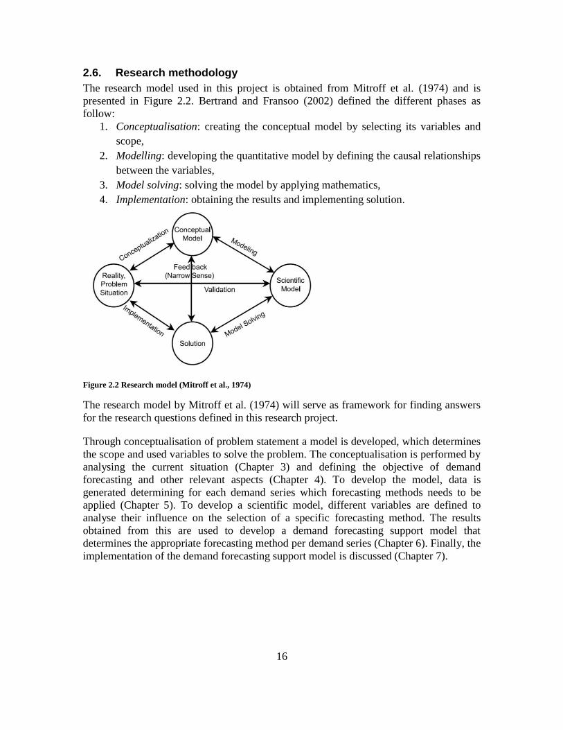
2.6. Research methodology
The research model used in this project is obtained from Mitroff et al. (1974) and is
presented in Figure 2.2. Bertrand and Fransoo (2002) defined the different phases as
follow:
1. Conceptualisation: creating the conceptual model by selecting its variables and
scope,
2. Modelling: developing the quantitative model by defining the causal relationships
between the variables,
3. Model solving: solving the model by applying mathematics,
4. Implementation: obtaining the results and implementing solution.
Figure 2.2 Research model (Mitroff et al., 1974)
The research model by Mitroff et al. (1974) will serve as framework for finding answers
for the research questions defined in this research project.
Through conceptualisation of problem statement a model is developed, which determines
the scope and used variables to solve the problem. The conceptualisation is performed by
analysing the current situation (Chapter 3) and defining the objective of demand
forecasting and other relevant aspects (Chapter 4). To develop the model, data is
generated determining for each demand series which forecasting methods needs to be
applied (Chapter 5). To develop a scientific model, different variables are defined to
analyse their influence on the selection of a specific forecasting method. The results
obtained from this are used to develop a demand forecasting support model that
determines the appropriate forecasting method per demand series (Chapter 6). Finally, the
implementation of the demand forecasting support model is discussed (Chapter 7).
17
3. Analysis of current situation
This chapter presents an overview of the current situation, discussing the demand and
customer characteristics. These characteristics are used to get insights in demand
forecasting at SABIC EUP. The data considered in this analysis are the sales data
between May 2010 and April 2011, considering the grades defined as mature by Business
Management. The grades classified as introduction, growth and end-of-life are not
considered in this research. These grades do not have (enough) representative historical
data available and require judgmental input. For these grades, the DCC has the task to
gather reliable information, which gives insights in future orders. It is assumed that the
sales data are a good approximation of demand during this period.
This chapter is organised as follows. Section 3.1 gives an overview of the demand
characteristics. Section 3.2 presents an analysis of the historical forecast accuracy to
present the historical performance. Finally, Section 3.3 discusses an additional
performance measurement, the forecast bias.
3.1. Demand characteristics
The first objective of this chapter is to give insights in the demand characteristics. As
discussed in Section 2.5, four VTs have been selected for this research project,
representing 48% of the total sold volume. A general overview of statistics is presented in
Table 3.1.
Table 3.1 Overview of general statistics per division
Division Value Team Average sales
per month (tons) St. dev. (tons)
No. of grades
No. of SKUs
No. of SKU+ warehouses
No. of SKU+ship-to’s
5 hdPE BM/Film ''''''''''''''''' ''''''''''''' 20 46 81 848
7-10 hdPE IM '''''''''''''' ''''''''''''''' 6 14 36 427
12 PP Copol ''''''''''''''' ''''''''''''' 31 75 83 1,272
14 PP Hopol ''''''''''''''' '''''''''''''' 41 80 122 1,267
Total
98 215 322 3,814
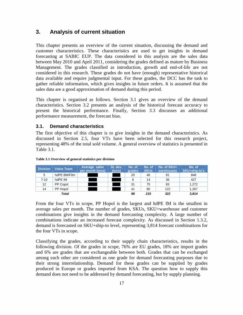
From the four VTs in scope, PP Hopol is the largest and hdPE IM is the smallest in
average sales per month. The number of grades, SKUs, SKU+warehouse and customer
combinations give insights in the demand forecasting complexity. A large number of
combinations indicate an increased forecast complexity. As discussed in Section 1.3.2,
demand is forecasted on SKU+ship-to level, representing 3,814 forecast combinations for
the four VTs in scope.
Classifying the grades, according to their supply chain characteristics, results in the
following division. Of the grades in scope, 76% are EU grades, 18% are import grades
and 6% are grades that are exchangeable between both. Grades that can be exchanged
among each other are considered as one grade for demand forecasting purposes due to
their strong interrelationship. Demand for these grades can be supplied by grades
produced in Europe or grades imported from KSA. The question how to supply this
demand does not need to be addressed by demand forecasting, but by supply planning.
18
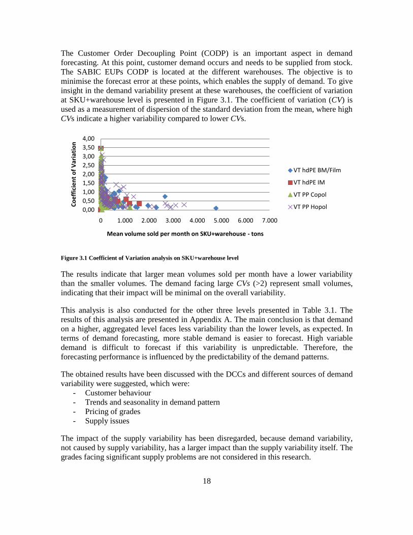
The Customer Order Decoupling Point (CODP) is an important aspect in demand
forecasting. At this point, customer demand occurs and needs to be supplied from stock.
The SABIC EUPs CODP is located at the different warehouses. The objective is to
minimise the forecast error at these points, which enables the supply of demand. To give
insight in the demand variability present at these warehouses, the coefficient of variation
at SKU+warehouse level is presented in Figure 3.1. The coefficient of variation (CV) is
used as a measurement of dispersion of the standard deviation from the mean, where high
CVs indicate a higher variability compared to lower CVs.
Figure 3.1 Coefficient of Variation analysis on SKU+warehouse level
The results indicate that larger mean volumes sold per month have a lower variability
than the smaller volumes. The demand facing large CVs (>2) represent small volumes,
indicating that their impact will be minimal on the overall variability.
This analysis is also conducted for the other three levels presented in Table 3.1. The
results of this analysis are presented in Appendix A. The main conclusion is that demand
on a higher, aggregated level faces less variability than the lower levels, as expected. In
terms of demand forecasting, more stable demand is easier to forecast. High variable
demand is difficult to forecast if this variability is unpredictable. Therefore, the
forecasting performance is influenced by the predictability of the demand patterns.
The obtained results have been discussed with the DCCs and different sources of demand
variability were suggested, which were:
- Customer behaviour
- Trends and seasonality in demand pattern
- Pricing of grades
- Supply issues
The impact of the supply variability has been disregarded, because demand variability,
not caused by supply variability, has a larger impact than the supply variability itself. The
grades facing significant supply problems are not considered in this research.
0,00
0,50
1,00
1,50
2,00
2,50
3,00
3,50
4,00
0 1.000 2.000 3.000 4.000 5.000 6.000 7.000
Co
eff
icie
nt
of
Var
iati
on
Mean volume sold per month on SKU+warehouse - tons
VT hdPE BM/Film
VT hdPE IM
VT PP Copol
VT PP Hopol
19
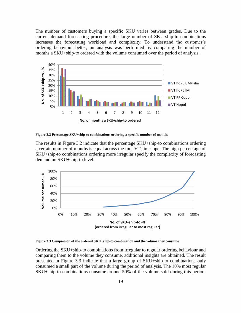
The number of customers buying a specific SKU varies between grades. Due to the
current demand forecasting procedure, the large number of SKU-ship-to combinations
increases the forecasting workload and complexity. To understand the customer‟s
ordering behaviour better, an analysis was performed by comparing the number of
months a SKU+ship-to ordered with the volume consumed over the period of analysis.
Figure 3.2 Percentage SKU+ship-to combinations ordering a specific number of months
The results in Figure 3.2 indicate that the percentage SKU+ship-to combinations ordering
a certain number of months is equal across the four VTs in scope. The high percentage of
SKU+ship-to combinations ordering more irregular specify the complexity of forecasting
demand on SKU+ship-to level.
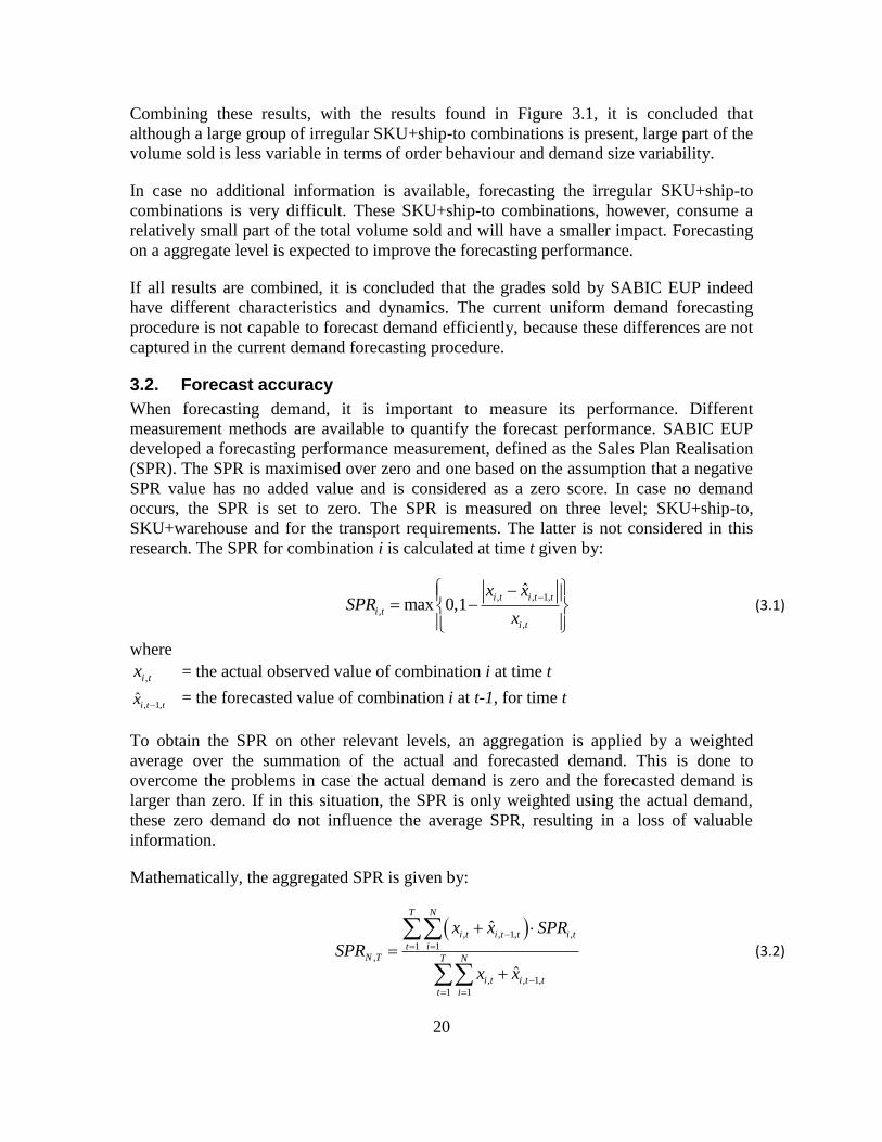
Figure 3.3 Comparison of the ordered SKU+ship-to combination and the volume they consume
Ordering the SKU+ship-to combinations from irregular to regular ordering behaviour and
comparing them to the volume they consume, additional insights are obtained. The result
presented in Figure 3.3 indicate that a large group of SKU+ship-to combinations only
consumed a small part of the volume during the period of analysis. The 10% most regular
SKU+ship-to combinations consume around 50% of the volume sold during this period.
0%
5%
10%
15%
20%
25%
30%
35%
40%
1 2 3 4 5 6 7 8 9 10 11 12
No
. of
SKU
+sh
ip-t
o -
%
No. of months a SKU+ship-to ordered
VT hdPE BM/Film
VT hdPE IM
VT PP Copol
VT Hopol
0%
20%
40%
60%
80%
100%
0% 10% 20% 30% 40% 50% 60% 70% 80% 90% 100%
Vo
lum
e c
on
sum
ed
-%
No. of SKU+ship-to -%(ordered from irregular to most regular)
20
Combining these results, with the results found in Figure 3.1, it is concluded that
although a large group of irregular SKU+ship-to combinations is present, large part of the
volume sold is less variable in terms of order behaviour and demand size variability.
In case no additional information is available, forecasting the irregular SKU+ship-to
combinations is very difficult. These SKU+ship-to combinations, however, consume a
relatively small part of the total volume sold and will have a smaller impact. Forecasting
on a aggregate level is expected to improve the forecasting performance.
If all results are combined, it is concluded that the grades sold by SABIC EUP indeed
have different characteristics and dynamics. The current uniform demand forecasting
procedure is not capable to forecast demand efficiently, because these differences are not
captured in the current demand forecasting procedure.
3.2. Forecast accuracy
When forecasting demand, it is important to measure its performance. Different
measurement methods are available to quantify the forecast performance. SABIC EUP
developed a forecasting performance measurement, defined as the Sales Plan Realisation
(SPR). The SPR is maximised over zero and one based on the assumption that a negative
SPR value has no added value and is considered as a zero score. In case no demand
occurs, the SPR is set to zero. The SPR is measured on three level; SKU+ship-to,
SKU+warehouse and for the transport requirements. The latter is not considered in this
research. The SPR for combination i is calculated at time t given by:
, , 1,
,
,
ˆmax 0,1
i t i t t
i t
i t
x xSPR
x
(3.1)
where
,i tx = the actual observed value of combination i at time t
, 1,ˆ
i t tx = the forecasted value of combination i at t-1, for time t
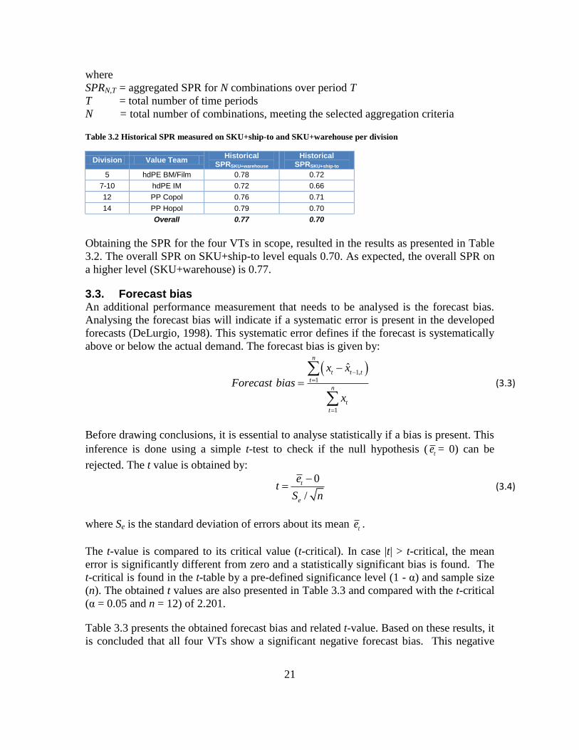
To obtain the SPR on other relevant levels, an aggregation is applied by a weighted
average over the summation of the actual and forecasted demand. This is done to
overcome the problems in case the actual demand is zero and the forecasted demand is
larger than zero. If in this situation, the SPR is only weighted using the actual demand,
these zero demand do not influence the average SPR, resulting in a loss of valuable
information.
Mathematically, the aggregated SPR is given by:
, , 1, ,
1 1,
, , 1,
1 1
ˆ
ˆ
T N
i t i t t i t
t iN T T N
i t i t t
t i
x x SPR
SPR
x x
(3.2)
21
where
SPRN,T = aggregated SPR for N combinations over period T T = total number of time periods
N = total number of combinations, meeting the selected aggregation criteria
Table 3.2 Historical SPR measured on SKU+ship-to and SKU+warehouse per division
Division Value Team Historical
SPRSKU+warehouse
Historical SPRSKU+ship-to
5 hdPE BM/Film 0.78 0.72
7-10 hdPE IM 0.72 0.66
12 PP Copol 0.76 0.71
14 PP Hopol 0.79 0.70
Overall 0.77 0.70
Obtaining the SPR for the four VTs in scope, resulted in the results as presented in Table
3.2. The overall SPR on SKU+ship-to level equals 0.70. As expected, the overall SPR on
a higher level (SKU+warehouse) is 0.77.
3.3. Forecast bias An additional performance measurement that needs to be analysed is the forecast bias.
Analysing the forecast bias will indicate if a systematic error is present in the developed
forecasts (DeLurgio, 1998). This systematic error defines if the forecast is systematically
above or below the actual demand. The forecast bias is given by:
1,
1
1
ˆ
n
t t t
t
n
t
t
x x
Forecast bias
x
(3.3)
Before drawing conclusions, it is essential to analyse statistically if a bias is present. This
inference is done using a simple t-test to check if the null hypothesis ( te = 0) can be
rejected. The t value is obtained by:
0
/
t
e
et
S n
(3.4)
where Se is the standard deviation of errors about its mean te .
The t-value is compared to its critical value (t-critical). In case |t| > t-critical, the mean
error is significantly different from zero and a statistically significant bias is found. The
t-critical is found in the t-table by a pre-defined significance level (1 - α) and sample size
(n). The obtained t values are also presented in Table 3.3 and compared with the t-critical
(α = 0.05 and n = 12) of 2.201.
Table 3.3 presents the obtained forecast bias and related t-value. Based on these results, it
is concluded that all four VTs show a significant negative forecast bias. This negative
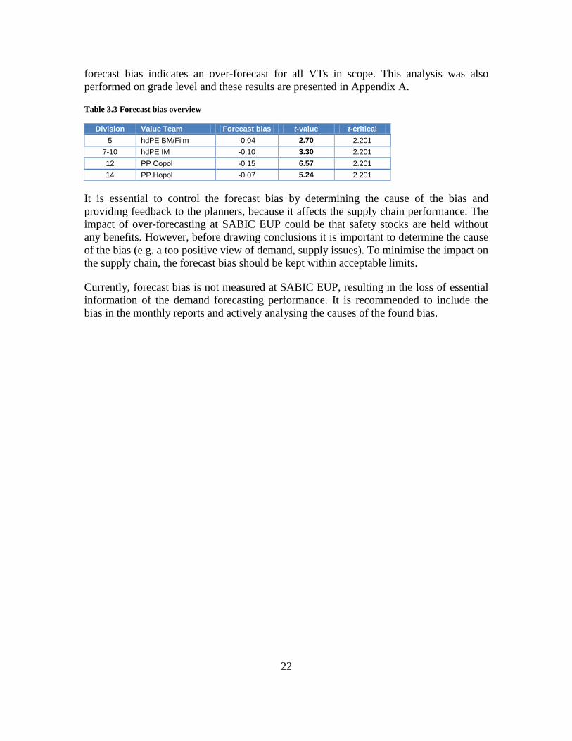
22
forecast bias indicates an over-forecast for all VTs in scope. This analysis was also
performed on grade level and these results are presented in Appendix A.
Table 3.3 Forecast bias overview
Division Value Team Forecast bias t-value t-critical
5 hdPE BM/Film -0.04 2.70 2.201
7-10 hdPE IM -0.10 3.30 2.201
12 PP Copol -0.15 6.57 2.201
14 PP Hopol -0.07 5.24 2.201
It is essential to control the forecast bias by determining the cause of the bias and
providing feedback to the planners, because it affects the supply chain performance. The
impact of over-forecasting at SABIC EUP could be that safety stocks are held without
any benefits. However, before drawing conclusions it is important to determine the cause
of the bias (e.g. a too positive view of demand, supply issues). To minimise the impact on
the supply chain, the forecast bias should be kept within acceptable limits.
Currently, forecast bias is not measured at SABIC EUP, resulting in the loss of essential
information of the demand forecasting performance. It is recommended to include the
bias in the monthly reports and actively analysing the causes of the found bias.
23
4. Methodology to determine best demand forecasts
The first research question is aimed at determining the best demand forecasts for SABIC
EUP, considering both the forecast level and method to develop these forecasts. This
chapter discusses the methodology used to determine the best demand forecasts for
SABIC EUP.
Before discussing the methodology, the objective of demand forecasting at SABIC EUP
is defined in Section 4.1. Forecasts can be developed applying different methods. For this
research project, a selection of relevant methods has been made and is presented in
Section 4.2. Another aspect in demand forecasting is the level at which the forecasts are
developed. Based on the supply chain of SABIC EUP, different levels have been defined
and are presented in Section 4.3. In case the forecast is developed on a higher, aggregated
level, a disaggregation needs to be applied. The method of disaggregation is discussed in
Section 4.4. Besides developing the forecasts, it is important to measure its performance.
The measurements used to quantify this performance are discussed in Section 4.5.
Finally, the methodology to investigate the best demand forecasts is discussed in Section
4.6.
4.1. Demand forecasting objective
As defined in Section 1.3.2, the objective of demand forecasting is to determine the
expected demand at the Customer Order Decoupling Point (CODP), where the products
are made-to-stock and used to supply demand. For SABIC EUP, the COPD is located at
the different warehouses. At these locations, incoming demand is fulfilled from stock.
The objective of the demand forecast is to determine the expected demand for each SKU
per warehouse (SKU+warehouse level). Considering SABIC EUPs supply chain, the
following distinction in grades is made:
- EU grades, which are stored in one warehouse, located near production plant
- Import grades, which are stored in seven warehouses (hubs), located across
Europe
Most EU grades are produced at one production location. After production, these grades
are stored at one warehouse location. The demand forecast must determine the expected
demand at this warehouse. The decision that has to be made is how much of each SKU
needs to be produced to maintain the optimal inventory level enabling the supply of
demand at minimum costs. The replenishment lead time for EU grades is one month,
meaning that production has yet to be planned for the upcoming month. For that reason,
the primary objective of forecasting the demand of EU grades is focused on minimising
the forecast over the upcoming month, defined as t+1, where t is the month at which the
forecast is made.
Import grades are supplied from seven warehouses located around Europe, where
customers are supplied from one warehouse based on minimising overall costs. In case of
supply issues, exceptions are made. The forecast needs to determine the demand for
import grades at each of the warehouses during the horizon of the replenishment of three

24
months. During this horizon, supply has been agreed upon for the period t+1 and t+2.
For period t+3, the supply is still open and depends on how much demand is expected at
t+1, t+2 and t+3. As a result, the priority of demand forecasting of import grades is to
minimise the forecast error over the horizon of these three months (h=3).
Grades that are exchangeable between EU and import are considered as one grade. The
supply for period t+1 and t+2 has already been confirmed for import. The priority for the
demand forecast is to minimise the error for the upcoming period (t+1), because the
supply for EU grades still needs to be planned and is the first decision that has to be
taken. For this period, it is still possible to steer the supply process such that demand can
be fulfilled. Note, that also a decision has to be made with regard how much import
grades are supplied at t+3. However, the demand forecast is optimised on t+1.
With this in mind, a model is developed to determine the best forecasting procedure,
considering the characteristics of SABIC EUP. The different aspects of this model are
presented in the upcoming sections.
4.2. Forecasting methods
Based on the demand analysis, different statistical forecasting methods are proposed to be
included in this research to investigate their applicability in demand forecasting. The
objective of this research is focused on developing a demand forecasting support model
with basic forecasting models, because complex statistical forecasting methods do not
necessarily perform better than simpler methods (Makridakis and Hibon, 2000). The
suggested relationship between the selling price of the product and the realised demand is
considered to be out of scope, based on interviews with employees at SABIC EUP. It was
concluded that selling price is influenced by a large set of variables and a model,
incorporating these variable in forecasting is considered too complex for this research
project. Later in this research, price variability will be considered to investigate the
difference between statistically and judgmentally forecasted demand. This is discussed in
Chapter 6. For future research, it could be interesting to investigate the relationship
between price and demand to develop a model that predicts the expected demand based
on the price strategy and its underlying variables.
For this research project, the following statistical forecasting methods are selected. Each
method is defined in detail in Appendix B:
- Random walk
- Simple moving average
- Single exponential smoothing
- Holt‟s linear exponential smoothing
- Seasonal exponential smoothing
- Winters‟ exponential smoothing
- Regression model
- Seasonal regression model
- Croston‟s model
- Adjusted Croston‟s model

25
Each of the above mentioned statistical forecasting methods is compared to the historical
demand forecast. This historical demand forecast is judgmentally developed, as discussed
in Section 1.3.2, and is defined as the judgmental forecasting method. This judgmental
forecasting method is added as one of the possible forecasting methods that can be
applied.
4.3. Levels of forecasting
From a variability pooling perspective, it would be interesting to investigate if forecasting
demand on an aggregated level results in a better performance on the required
information level. Demand can also be forecasted on a lower level to better grasp all
details. This forecast is then aggregated to the required information level. Both options
are only allowed if the forecast accuracy is improved on SKU+warehouse level.
In this research project, the demand forecast needs to determine the expected demand for
each SKU at the different stock points (warehouses). Considering the characteristics of
the supply chain of SABIC EUP, the following relevant forecast levels are suggested:
- Grade level
- SKU level
- SKU+warehouse level
- SKU+ship-to level
The highest levels are selected from a production perspective. Demand can be forecasted
per grade and by including the packaging type, per SKU. The third level is the level on
which the demand forecast needs to be optimised. The final and most detailed level is
aimed at forecasting demand for a specific SKU per customer. This level is defined as the
SKU+ship-to level. Recall from Section 1.3.2, that currently demand is forecasted
judgmentally on this SKU+ship-to level.
In theory, a clear link exists between all forecast levels, where a grade exists of multiple
SKUs. These SKUs are delivered from one or more warehouses to one or more
customers. A customer is assigned to a specific warehouse from which he is supplied
with the specific SKU, minimising the transportation costs. In practice, it appears that
customers are sometimes supplied from multiple warehouses, due to different reasons
(e.g. supply issues, inventory management). The link between a customer and its
predefined warehouse is not saved and therefore this link cannot be obtained. For this
research, this link is obtained from the realised data, containing which warehouse
supplied the customer‟s demand. It occurs rarely that a customer is supplied from
multiple warehouses and represents 4% of the total volume. The impact of this volume is
assumed to be negligible.
4.4. Disaggregation method
In case demand is forecasted on a higher, aggregated level, it is necessary to disaggregate
the demand forecast to the required lower levels. Different disaggregation methods exist
and in a research by Gross and Sohl (1990), 21 of such methods were examined. They
concluded that the mean-proportional disaggregation method is the simplest and still
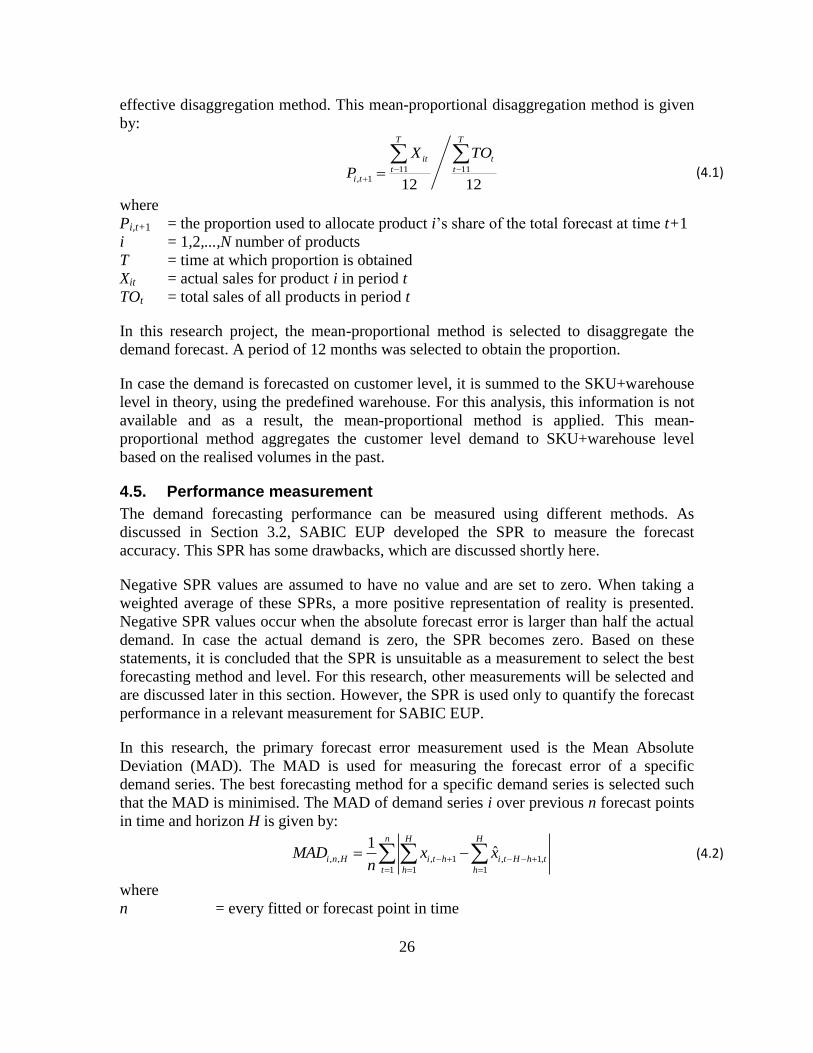
26
effective disaggregation method. This mean-proportional disaggregation method is given
by:
11 11, 1
12 12
T T
it t
t ti t
X TO
P
(4.1)
where
Pi,t+1 = the proportion used to allocate product i‟s share of the total forecast at time t+1
i = 1,2,...,N number of products
T = time at which proportion is obtained
Xit = actual sales for product i in period t
TOt = total sales of all products in period t
In this research project, the mean-proportional method is selected to disaggregate the
demand forecast. A period of 12 months was selected to obtain the proportion.
In case the demand is forecasted on customer level, it is summed to the SKU+warehouse
level in theory, using the predefined warehouse. For this analysis, this information is not
available and as a result, the mean-proportional method is applied. This mean-
proportional method aggregates the customer level demand to SKU+warehouse level
based on the realised volumes in the past.
4.5. Performance measurement
The demand forecasting performance can be measured using different methods. As
discussed in Section 3.2, SABIC EUP developed the SPR to measure the forecast
accuracy. This SPR has some drawbacks, which are discussed shortly here.
Negative SPR values are assumed to have no value and are set to zero. When taking a
weighted average of these SPRs, a more positive representation of reality is presented.
Negative SPR values occur when the absolute forecast error is larger than half the actual
demand. In case the actual demand is zero, the SPR becomes zero. Based on these
statements, it is concluded that the SPR is unsuitable as a measurement to select the best
forecasting method and level. For this research, other measurements will be selected and
are discussed later in this section. However, the SPR is used only to quantify the forecast
performance in a relevant measurement for SABIC EUP.
In this research, the primary forecast error measurement used is the Mean Absolute
Deviation (MAD). The MAD is used for measuring the forecast error of a specific
demand series. The best forecasting method for a specific demand series is selected such
that the MAD is minimised. The MAD of demand series i over previous n forecast points
in time and horizon H is given by:
, , , 1 , 1,
1 1 1
1ˆ
n H H
i n H i t h i t H h t
t h h
MAD x xn
(4.2)
where
n = every fitted or forecast point in time
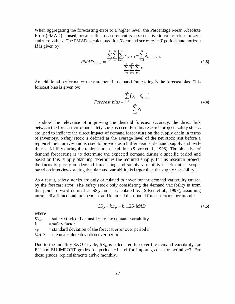
27
When aggregating the forecasting error to a higher level, the Percentage Mean Absolute
Error (PMAD) is used, because this measurement is less sensitive to values close to zero
and zero values. The PMAD is calculated for N demand series over T periods and horizon
H is given by:
, 1 , 1,
1 1 1 1
, ,
,
1 1 1
ˆT N H H
i t h i t H h t
t i h h
N T H T N H
i t
t i h
x x
PMAD
x
(4.3)
An additional performance measurement in demand forecasting is the forecast bias. This
forecast bias is given by:
1,
1
1
ˆ
n
t t t
t
n
t
t
x x
Forecast bias
x
(4.4)
To show the relevance of improving the demand forecast accuracy, the direct link
between the forecast error and safety stock is used. For this research project, safety stocks
are used to indicate the direct impact of demand forecasting on the supply chain in terms
of inventory. Safety stock is defined as the average level of the net stock just before a
replenishment arrives and is used to provide as a buffer against demand, supply and lead-
time variability during the replenishment lead time (Silver et al., 1998). The objective of
demand forecasting is to determine the expected demand during a specific period and
based on this, supply planning determines the required supply. In this research project,
the focus is purely on demand forecasting and supply variability is left out of scope,
based on interviews stating that demand variability is larger than the supply variability.
As a result, safety stocks are only calculated to cover for the demand variability caused
by the forecast error. The safety stock only considering the demand variability is from
this point forward defined as SSD and is calculated by (Silver et al., 1998), assuming
normal distributed and independent and identical distributed forecast errors per month:
1.25D DSS k k MAD (4.5)
where
SSD = safety stock only considering the demand variability
k = safety factor
σD = standard deviation of the forecast error over period t
MAD = mean absolute deviation over period t
Due to the monthly S&OP cycle, SSD is calculated to cover the demand variability for
EU and EU/IMPORT grades for period t+1 and for import grades for period t+3. For
these grades, replenishments arrive monthly.
28
4.6. Methodology
To determine the best demand forecasts, both the forecast level and method are
considered. For each demand series, the best statistical forecasting method is determined
and compared to the historical judgmental forecast. Based on this comparison the best
forecasting method obtained. If this statistical forecast outperforms or equals the
judgmental forecast, it is preferred over the judgmental forecast.
The next question is on what level demand needs to be forecasted. By developing
forecast on different levels and (dis)aggregating them correctly, the forecast performance
can be analysed on SKU+warehouse level to determine the best forecast level. Three
scenarios are considered here:
1. Determine the forecast performance when the best forecast level is selected per
grade and each demand series is forecasted using the best forecasting method.
2. Determine the forecast performance when one forecast level is applied for all
grades. Each demand series is forecasted using the best forecasting method.
3. Determine the forecast performance when only statistical forecasting methods are
considered.
Applying multiple forecast levels is considered to increase the complexity of the
procedure. For that reason, the second scenario is considered to determine the difference
in forecasting performance, when the complexity is reduced. The final scenario is
selected to develop insights in the benefit of judgmental forecasting by only considering
statistical methods.
The selected period of analysis ranges from May 2009 until April 2011. Due to the
financial crisis of 2008, which ended in the first quarter of 2009, no data have been
selected from this period, because this period is not representative for the current business
situation. The total sample of 24 months is divided into two periods, where the first 12
months are used to initialise and fit the parameters of the different models, minimising
the MAD. The last 12 months are used to analyse the forecast performance of these
models. Over this period, the best statistical forecast is compared to the judgmental
forecast for every demand series. The forecast methods that realises the smallest MAD
over these 12 months is selected as the best forecast method.
The length of the initialisation period depends on the model applied. Level models
require an initialisation period of one month, where trend models require an initialisation
period of four months. In case of the seasonal and Winters‟ exponential smoothing, 12 to
15 months of initialisation is required, respectively. Compared to the level and trend
models, seasonal models require more data for initialisation, which is a drawback of these
models. As for this research project, the objective is to determine under which
circumstances a specific forecast method is better compared to other methods, it is
required to use the same period to measure the forecast performance. For this purpose,
extra data have been selected from February 2007 until April 2008 to initialise these
seasonal models enabling an equal comparison. Based on input from demand planners at
SABIC EUP, this period is considered representative for business nowadays. Only using
this data for the seasonal methods gives them a slight advantage. This advantage is
29
assumed negligible, because fitting the different parameters of the models is done over
more or less the same data set.
Currently, the initial judgmental forecasts are not saved, which makes comparison
impossible. To make a comparison possible, the agreed demand forecasts after the S&OP
meeting are defined as the judgmental forecast, as they are largely based on the initial
judgmental forecasts. For future research, it is important to save the initial forecast as
well to be able to determine the differences between the initial and agreed demand
forecast. Due to a system error, the judgmental forecast data has been lost between
October 2009 and April 2010, which makes a comparison of the methods with the
judgmental forecast impossible over this period.
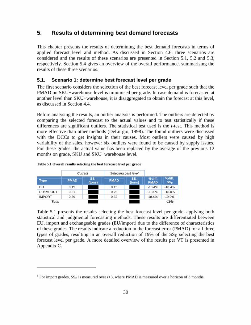
30
5. Results of determining best demand forecasts
This chapter presents the results of determining the best demand forecasts in terms of
applied forecast level and method. As discussed in Section 4.6, three scenarios are
considered and the results of these scenarios are presented in Section 5.1, 5.2 and 5.3,
respectively. Section 5.4 gives an overview of the overall performance, summarising the
results of these three scenarios.
5.1. Scenario 1: determine best forecast level per grade
The first scenario considers the selection of the best forecast level per grade such that the
PMAD on SKU+warehouse level is minimised per grade. In case demand is forecasted at
another level than SKU+warehouse, it is disaggregated to obtain the forecast at this level,
as discussed in Section 4.4.
Before analysing the results, an outlier analysis is performed. The outliers are detected by
comparing the selected forecast to the actual values and to test statistically if these
differences are significant outliers. The statistical test used is the t-test. This method is
more effective than other methods (DeLurgio, 1998). The found outliers were discussed
with the DCCs to get insights in their causes. Most outliers were caused by high
variability of the sales, however six outliers were found to be caused by supply issues.
For these grades, the actual value has been replaced by the average of the previous 12
months on grade, SKU and SKU+warehouse level.
Table 5.1 Overall results selecting the best forecast level per grade
Current Selecting best level
Type PMAD SSD
(tons) PMAD
SSD (tons)
%diff. PMAD
%diff. SSD
EU 0.19 ''''''''''''''''' 0.15 '''''''''''''''' -18.4% -18.4%
EU/IMPORT 0.31 ''''''''''''''''' 0.25 '''''''''''''''' -18.0% -18.0%
IMPORT 0.39 ''''''''''''''' 0.32 '''''''''''''''' -18.4%1 -19.9%
1
Total '''''''''''''
'''''''''''''
-19%
Table 5.1 presents the results selecting the best forecast level per grade, applying both
statistical and judgmental forecasting methods. These results are differentiated between
EU, import and exchangeable grades (EU/import) due to the difference of characteristics
of these grades. The results indicate a reduction in the forecast error (PMAD) for all three
types of grades, resulting in an overall reduction of 19% of the SSD selecting the best
forecast level per grade. A more detailed overview of the results per VT is presented in
Appendix C.
1 For import grades, SSD is measured over t+3, where PMAD is measured over a horizon of 3 months
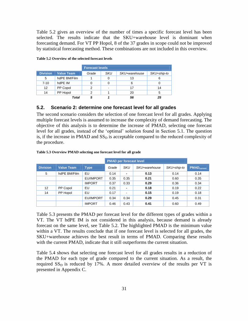
31
Table 5.2 gives an overview of the number of times a specific forecast level has been
selected. The results indicate that the SKU+warehouse level is dominant when
forecasting demand. For VT PP Hopol, 8 of the 37 grades in scope could not be improved
by statistical forecasting method. These combinations are not included in this overview.
Table 5.2 Overview of the selected forecast levels
Forecast levels
Division Value Team Grade SKU SKU+warehouse SKU+ship-to
5 hdPE BM/Film 1 0 13 6
7-10 hdPE IM 0 0 6 0
12 PP Copol 2 - 17 14
14 PP Hopol 2 1 20 5
Total 5 1 56 25
5.2. Scenario 2: determine one forecast level for all grades
The second scenario considers the selection of one forecast level for all grades. Applying
multiple forecast levels is assumed to increase the complexity of demand forecasting. The
objective of this analysis is to determine the increase of PMAD, selecting one forecast
level for all grades, instead of the „optimal‟ solution found in Section 5.1. The question
is, if the increase in PMAD and SSD is acceptable compared to the reduced complexity of
the procedure.
Table 5.3 Overview PMAD selecting one forecast level for all grade
PMAD per forecast level
Division Value Team Type Grade SKU SKU+warehouse SKU+ship-to PMADcurrent
5 hdPE BM/Film EU 0.14 - 0.13 0.14 0.14
EU/IMPORT 0.35 0.35 0.21 0.60 0.35
IMPORT 0.37 0.33 0.29 0.36 0.34
12 PP Copol EU 0.21 - 0.18 0.19 0.22
14 PP Hopol EU 0.17 - 0.15 0.19 0.18
EU/IMPORT 0.34 0.34 0.29 0.45 0.31
IMPORT 0.46 0.43 0.41 0.60 0.49
Table 5.3 presents the PMAD per forecast level for the different types of grades within a
VT. The VT hdPE IM is not considered in this analysis, because demand is already
forecast on the same level, see Table 5.2. The highlighted PMAD is the minimum value
within a VT. The results conclude that if one forecast level is selected for all grades, the
SKU+warehouse achieves the best result in terms of PMAD. Comparing these results
with the current PMAD, indicate that it still outperforms the current situation.
Table 5.4 shows that selecting one forecast level for all grades results in a reduction of
the PMAD for each type of grade compared to the current situation. As a result, the
required SSD is reduced by 17%. A more detailed overview of the results per VT is
presented in Appendix C.
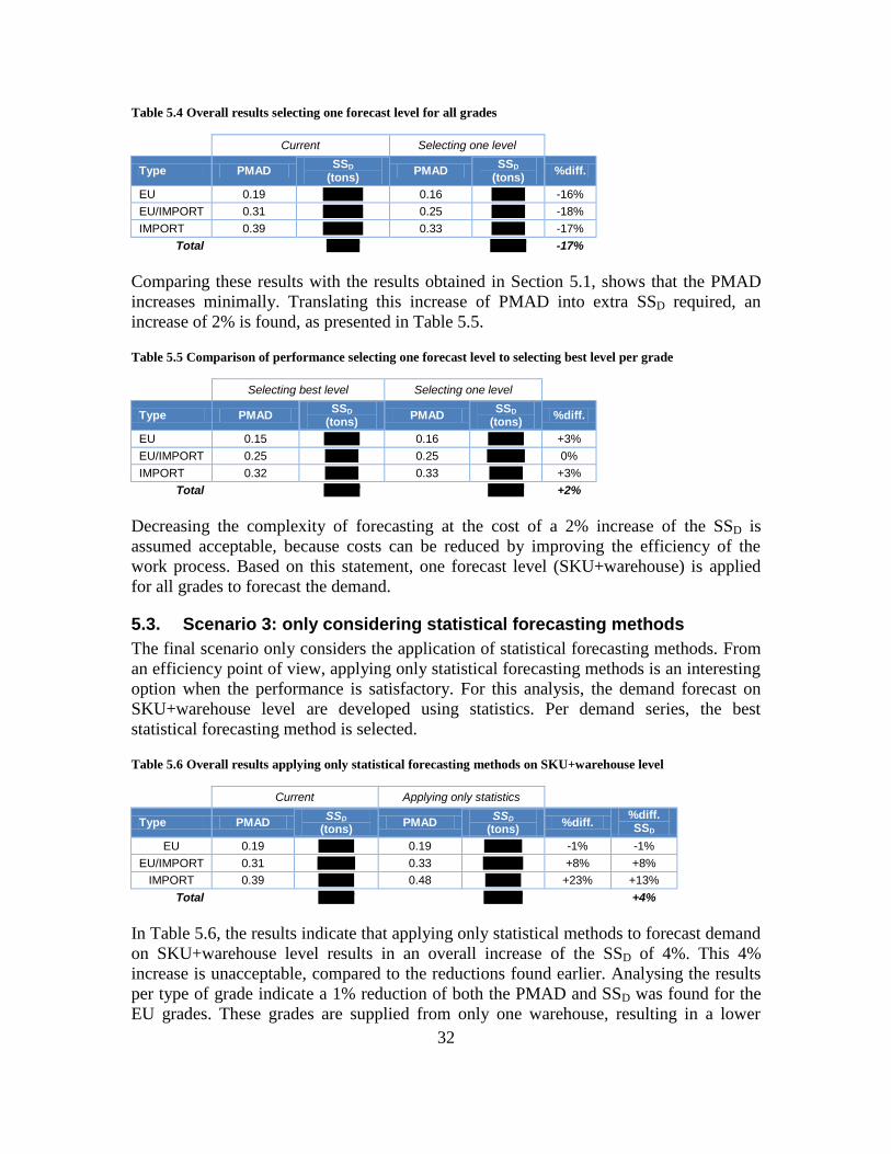
32
Table 5.4 Overall results selecting one forecast level for all grades
Current Selecting one level
Type PMAD SSD
(tons) PMAD
SSD (tons)
%diff.
EU 0.19 '''''''''''''''''' 0.16 ''''''''''''''' -16%
EU/IMPORT 0.31 '''''''''''''''''' 0.25 ''''''''''''''' -18%
IMPORT 0.39 '''''''''''''''''' 0.33 ''''''''''''''' -17%
Total
''''''''''''
''''''''''''' -17%
Comparing these results with the results obtained in Section 5.1, shows that the PMAD
increases minimally. Translating this increase of PMAD into extra SSD required, an
increase of 2% is found, as presented in Table 5.5.
Table 5.5 Comparison of performance selecting one forecast level to selecting best level per grade
Selecting best level Selecting one level
Type PMAD SSD
(tons) PMAD
SSD (tons)
%diff.
EU 0.15 '''''''''''''''' 0.16 '''''''''''''''' +3%
EU/IMPORT 0.25 ''''''''''''''' 0.25 ''''''''''''''''' 0%
IMPORT 0.32 ''''''''''''''' 0.33 ''''''''''''''' +3%
Total
'''''''''''''
''''''''''''' +2%
Decreasing the complexity of forecasting at the cost of a 2% increase of the SSD is
assumed acceptable, because costs can be reduced by improving the efficiency of the
work process. Based on this statement, one forecast level (SKU+warehouse) is applied
for all grades to forecast the demand.
5.3. Scenario 3: only considering statistical forecasting methods
The final scenario only considers the application of statistical forecasting methods. From
an efficiency point of view, applying only statistical forecasting methods is an interesting
option when the performance is satisfactory. For this analysis, the demand forecast on
SKU+warehouse level are developed using statistics. Per demand series, the best
statistical forecasting method is selected.
Table 5.6 Overall results applying only statistical forecasting methods on SKU+warehouse level
Current Applying only statistics
Type PMAD SSD
(tons) PMAD
SSD
(tons) %diff.
%diff. SSD
EU 0.19 '''''''''''''''' 0.19 ''''''''''''''''' -1% -1%
EU/IMPORT 0.31 ''''''''''''''''' 0.33 '''''''''''''''''' +8% +8%
IMPORT 0.39 '''''''''''''''' 0.48 '''''''''''''''' +23% +13%
Total '''''''''''''
''''''''''''''
+4%
In Table 5.6, the results indicate that applying only statistical methods to forecast demand
on SKU+warehouse level results in an overall increase of the SSD of 4%. This 4%
increase is unacceptable, compared to the reductions found earlier. Analysing the results
per type of grade indicate a 1% reduction of both the PMAD and SSD was found for the
EU grades. These grades are supplied from only one warehouse, resulting in a lower
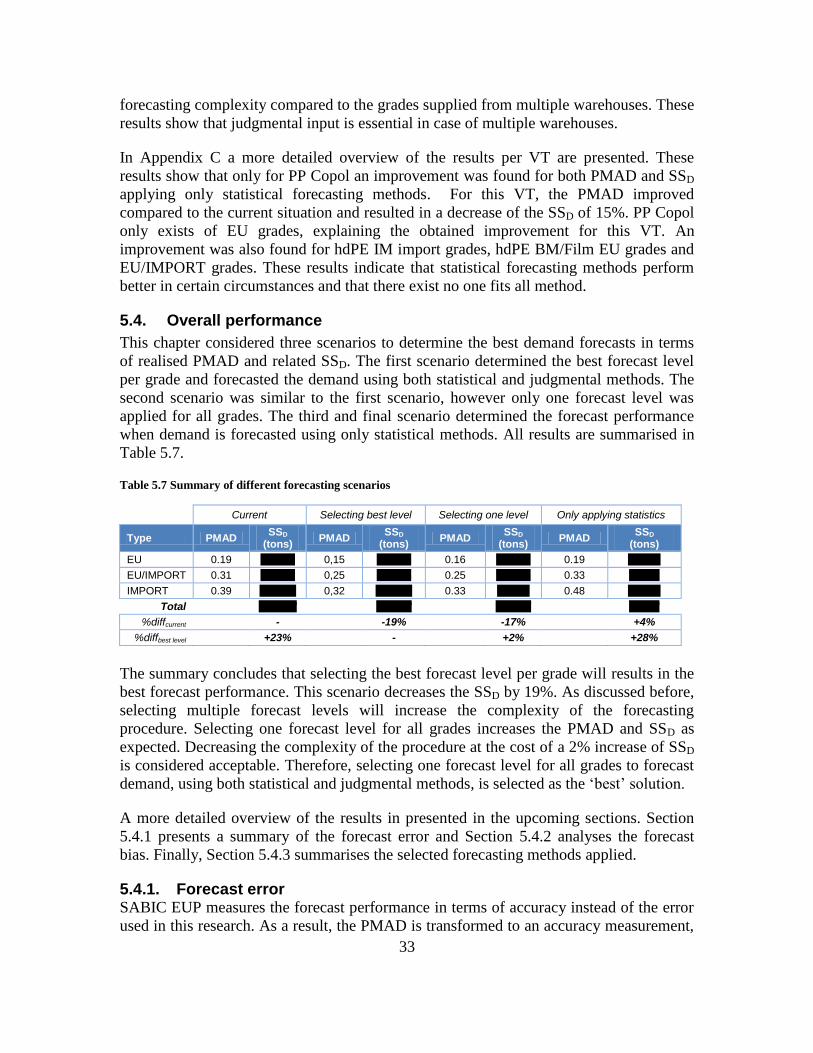
33
forecasting complexity compared to the grades supplied from multiple warehouses. These
results show that judgmental input is essential in case of multiple warehouses.
In Appendix C a more detailed overview of the results per VT are presented. These
results show that only for PP Copol an improvement was found for both PMAD and SSD
applying only statistical forecasting methods. For this VT, the PMAD improved
compared to the current situation and resulted in a decrease of the SSD of 15%. PP Copol
only exists of EU grades, explaining the obtained improvement for this VT. An
improvement was also found for hdPE IM import grades, hdPE BM/Film EU grades and
EU/IMPORT grades. These results indicate that statistical forecasting methods perform
better in certain circumstances and that there exist no one fits all method.
5.4. Overall performance
This chapter considered three scenarios to determine the best demand forecasts in terms
of realised PMAD and related SSD. The first scenario determined the best forecast level
per grade and forecasted the demand using both statistical and judgmental methods. The
second scenario was similar to the first scenario, however only one forecast level was
applied for all grades. The third and final scenario determined the forecast performance
when demand is forecasted using only statistical methods. All results are summarised in
Table 5.7.
Table 5.7 Summary of different forecasting scenarios
Current Selecting best level Selecting one level Only applying statistics
Type PMAD SSD
(tons) PMAD
SSD
(tons) PMAD
SSD
(tons) PMAD
SSD
(tons)
EU 0.19 ''''''''''''''''' 0,15 ''''''''''''''''' 0.16 ''''''''''''''''' 0.19 ''''''''''''''''
EU/IMPORT 0.31 ''''''''''''''''' 0,25 ''''''''''''''''' 0.25 ''''''''''''''''' 0.33 '''''''''''''''
IMPORT 0.39 '''''''''''''''''' 0,32 '''''''''''''''''' 0.33 '''''''''''''''' 0.48 ''''''''''''''''
Total
'''''''''''''''
''''''''''''''
''''''''''''''
''''''''''''
%diffcurrent -
-19%
-17%
+4%
%diffbest level +23%
-
+2%
+28%
The summary concludes that selecting the best forecast level per grade will results in the
best forecast performance. This scenario decreases the SSD by 19%. As discussed before,
selecting multiple forecast levels will increase the complexity of the forecasting
procedure. Selecting one forecast level for all grades increases the PMAD and SSD as
expected. Decreasing the complexity of the procedure at the cost of a 2% increase of SSD
is considered acceptable. Therefore, selecting one forecast level for all grades to forecast
demand, using both statistical and judgmental methods, is selected as the „best‟ solution.
A more detailed overview of the results in presented in the upcoming sections. Section
5.4.1 presents a summary of the forecast error and Section 5.4.2 analyses the forecast
bias. Finally, Section 5.4.3 summarises the selected forecasting methods applied.
5.4.1. Forecast error SABIC EUP measures the forecast performance in terms of accuracy instead of the error
used in this research. As a result, the PMAD is transformed to an accuracy measurement,
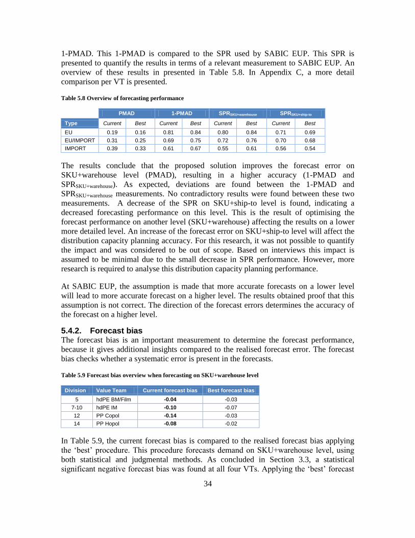
34
1-PMAD. This 1-PMAD is compared to the SPR used by SABIC EUP. This SPR is
presented to quantify the results in terms of a relevant measurement to SABIC EUP. An
overview of these results in presented in Table 5.8. In Appendix C, a more detail
comparison per VT is presented.
Table 5.8 Overview of forecasting performance
PMAD 1-PMAD SPRSKU+warehouse SPRSKU+ship-to
Type Current Best Current Best Current Best Current Best
EU 0.19 0.16 0.81 0.84 0.80 0.84 0.71 0.69
EU/IMPORT 0.31 0.25 0.69 0.75 0.72 0.76 0.70 0.68
IMPORT 0.39 0.33 0.61 0.67 0.55 0.61 0.56 0.54
The results conclude that the proposed solution improves the forecast error on
SKU+warehouse level (PMAD), resulting in a higher accuracy (1-PMAD and
SPRSKU+warehouse). As expected, deviations are found between the 1-PMAD and
SPRSKU+warehouse measurements. No contradictory results were found between these two
measurements. A decrease of the SPR on SKU+ship-to level is found, indicating a
decreased forecasting performance on this level. This is the result of optimising the
forecast performance on another level (SKU+warehouse) affecting the results on a lower
more detailed level. An increase of the forecast error on SKU+ship-to level will affect the
distribution capacity planning accuracy. For this research, it was not possible to quantify
the impact and was considered to be out of scope. Based on interviews this impact is
assumed to be minimal due to the small decrease in SPR performance. However, more
research is required to analyse this distribution capacity planning performance.
At SABIC EUP, the assumption is made that more accurate forecasts on a lower level
will lead to more accurate forecast on a higher level. The results obtained proof that this
assumption is not correct. The direction of the forecast errors determines the accuracy of
the forecast on a higher level.
5.4.2. Forecast bias The forecast bias is an important measurement to determine the forecast performance,
because it gives additional insights compared to the realised forecast error. The forecast
bias checks whether a systematic error is present in the forecasts.
Table 5.9 Forecast bias overview when forecasting on SKU+warehouse level
Division Value Team Current forecast bias Best forecast bias
5 hdPE BM/Film -0.04 -0.03
7-10 hdPE IM -0.10 -0.07
12 PP Copol -0.14 -0.03
14 PP Hopol -0.08 -0.02
In Table 5.9, the current forecast bias is compared to the realised forecast bias applying
the „best‟ procedure. This procedure forecasts demand on SKU+warehouse level, using
both statistical and judgmental methods. As concluded in Section 3.3, a statistical
significant negative forecast bias was found at all four VTs. Applying the „best‟ forecast
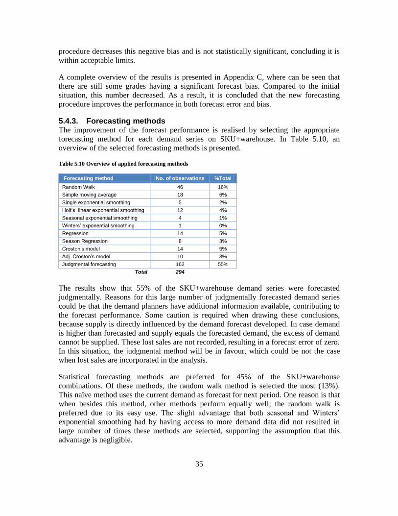
35
procedure decreases this negative bias and is not statistically significant, concluding it is
within acceptable limits.
A complete overview of the results is presented in Appendix C, where can be seen that
there are still some grades having a significant forecast bias. Compared to the initial
situation, this number decreased. As a result, it is concluded that the new forecasting
procedure improves the performance in both forecast error and bias.
5.4.3. Forecasting methods The improvement of the forecast performance is realised by selecting the appropriate
forecasting method for each demand series on SKU+warehouse. In Table 5.10, an
overview of the selected forecasting methods is presented.
Table 5.10 Overview of applied forecasting methods
Forecasting method No. of observations %Total
Random Walk 46 16%
Simple moving average 18 6%
Single exponential smoothing 5 2%
Holt’s linear exponential smoothing 12 4%
Seasonal exponential smoothing 4 1%
Winters’ exponential smoothing 1 0%
Regression 14 5%
Season Regression 8 3%
Croston’s model 14 5%
Adj. Croston’s model 10 3%
Judgmental forecasting 162 55%
Total 294
The results show that 55% of the SKU+warehouse demand series were forecasted
judgmentally. Reasons for this large number of judgmentally forecasted demand series
could be that the demand planners have additional information available, contributing to
the forecast performance. Some caution is required when drawing these conclusions,
because supply is directly influenced by the demand forecast developed. In case demand
is higher than forecasted and supply equals the forecasted demand, the excess of demand
cannot be supplied. These lost sales are not recorded, resulting in a forecast error of zero.
In this situation, the judgmental method will be in favour, which could be not the case
when lost sales are incorporated in the analysis.
Statistical forecasting methods are preferred for 45% of the SKU+warehouse
combinations. Of these methods, the random walk method is selected the most (13%).
This naïve method uses the current demand as forecast for next period. One reason is that
when besides this method, other methods perform equally well; the random walk is
preferred due to its easy use. The slight advantage that both seasonal and Winters‟
exponential smoothing had by having access to more demand data did not resulted in
large number of times these methods are selected, supporting the assumption that this
advantage is negligible.
36
6. Development of demand forecasting support model
The second research question is aimed at developing a support model that can be used in
demand forecasting. The purpose of this support model is to classify demand series
according to its characteristics and to determine which forecasting method needs to be
applied. In the previous chapter, the best forecasting methods have been determined per
demand series on SKU+warehouse level, resulting in a 17% decrease of the SSD. This
decrease gives an indication of the potential of applying both statistical and judgmental
forecasting methods. The question still unanswered is in what situation a specific
forecasting method needs to be applied. To find an answer to this question, the obtained
results from Chapter 5 are analysed statistically to develop a support model.
In the upcoming sections, the development and results of the support model are
discussed. A list of variables is presented that are suggested to discriminate between the
different forecasting methods in Section 6.1. These variables are defined as classification
variables. Section 6.2 discusses the analysis method and results when demand is
classified requiring either statistical or judgmental forecasting methods. In case only
statistical forecasting methods are considered, how could the demand series be classified
taking into account these methods and the suggested classification variables? This is
discussed in Section 6.3. Finally, the demand forecasting support model is presented in
Section 6.4 to summarise the results.
6.1. Suggested classification variables
To develop a demand forecasting support model, a list of possible classification variables
is defined that might explain the selection of a forecasting method over another method.
These variables are selected by combining the results of brainstorm sessions with the
DCCs, the supply chain structure of SABIC EUP, available literature in demand
categorisation and comparing the application of statistical and judgmental forecasting,
resulting in the following types of variables:
- Demand variability
On SKU+warehouse level
On SKU+ship-to level
- Presence of specific demand patterns
Trend factor
Seasonality
- Exclusive business information
Price variability
Out-of-stock situations
Changes to distribution network (from which warehouse a customer is
supplied)
Customer‟s characteristics
One of the essential aspects in forecasting is the ability to predict variability. Demand
variability can be defined in terms of volume, demand size and inter-arrival time. An
example of a research in this area is the paper by Syntetos et al. (2005), who used the
37
squared CV of the order size and the average inter-demand arrival time of demand to
categorise demand analytically between four statistical forecasting methods, considering
level demand. For this research project, the mean and CV for both the volume and
demand size of a demand series and the inter-arrival time of monthly demand on
SKU+warehouse level are selected. The mean and CV of the order size and inter-arrival
time of monthly demand on SKU+ship-to level is included in the analyses as well to
incorporate a customer‟s perspective.
Another aspect in forecasting is to ability to predict demand patterns (e.g. level, trend or
seasonal). The results in Table 5.10 indicated that 9% of the demand series on
SKU+warehouse level required a statistical forecasting method, assuming trend. Only 4%
of these series required a statistical forecasting method assuming seasonality. The
presence of a trend or seasonal pattern could explain the selection of a specific
forecasting method. However, due to the small number of seasonal demand series only
the trend factor is included as a possible classification variable.
The final aspect is the difference between statistical and judgmental forecasting. In
general, judgmental forecasting has an advantage in case exclusive business information
is available which is not available for statistical methods (Goodwin, 2002). Expected
business information contributing to the performance of judgmental forecasting are
known price variability, out-of-stock situations known in advance, changes in the
distribution network of products to the customers and the characteristics of these
customers. At this moment, the data of known out-of-stock situations and distribution
network changes are not available, making it impossible to include these variables in the
analysis. Recording this information in the future would enable research incorporating
these variables. The price variability of a grade is defined in terms of the CV of the
historical price without trend. The trend of increasing raw material prices is excluded,
because it is not of interest for this research. For each SKU+warehouse combination, the
number of customers and the percentage representing the average order size a SKU+ship-
to orders compared to the average monthly demand size of a SKU+warehouse
combination.
An overview of the suggested classification variables is as follow. The mathematical
formulas behind these variables are presented in Appendix D.
w = a specific SKU+warehouse combination
volumex w = average monthly demand at w
volumeCV w = coefficient of variation of monthly demand at w
demandx w = average monthly demand size, when occurring, at w
demandCV w = coefficient of variation of monthly demand size, when occurring at w
I w = average inter-arrival time of monthly demand at w
C w = the number of SKU+ship-to combinations supplied from w
orderx C w = average monthly order size of C(w)
38
orderCV C w = coefficient of variation of monthly order size of C(w)
I C w = average inter-arrival time of monthly demand of C(w)
p C w = percentage order size that C(w) orders of monthly demand size of w
b(w) = trend factor of demand series at w
CVprice(i) = coefficient of variation of invoiced price per grade i
Recall from Chapter 3, that this analysis only considers the mature grades. The grades
classified in the introduction, growth or end-of-life stage needs to be forecasted
judgmentally. In other words, the product life cycle status is the first classification
variable already applied. Each classification variable is defined for the demand on
SKU+warehouse level.
6.2. Statistical versus judgmental forecasting
In Chapter 5, the best methods have been determined for each demand series at
SKU+warehouse level to forecast the demand. The next step is to investigate whether
statistically significant differences exist between the demand forecasted by statistics or
judgment, such that procedures can be develop to classify demand accordingly.
6.2.1. Method of analysis Two different statistical techniques are available to conduct such an analysis. The first
technique, the discriminant analysis, derives a variate to discriminate best between
objects in the predefined groups (Hair et al., 2006). This variate is a linear combination of
two or more independent variables. The second technique is the logistic regression, which
is a specialised form of regression and is used to predict and explain a binary categorical
variable (Hair et al., 2006).
The main difference between these two techniques is that logistic regression can only be
applied in case of a binary dependent variable, where discriminant analysis can be used to
investigate dependent variables consisting of two or more values. The discriminant
analysis requires also some critical assumptions, like multivariate normality of the
independent variables and equality of the covariance matrices for the groups (Hair et al.,
2006). In case these assumptions are violated, the outcome is biased and alternative
methods should be considered (Hair et al., 2006). Logistic regression is much more
robust and does not require such assumptions, which makes this technique preferable
when considering only two groups. When the objective is to classify demand forecasted
by statistical or judgmental methods, logistic regression is preferred based on these
arguments.
For the logistic regression, the dependent variable FORECAST consists of two values;
statistical (0) and judgmental (1). The classification variables discussed in Section 6.1 are
selected as independent variables. The total sample consists of 275 observations (150 –
statistical and 125 – judgmental). To be able to validate the logistic regression model, the
sample has been divided into two random subsamples. One subsample is used to estimate
the parameters to develop the logistic regression model. The other subsample is used to
validate this model by assessing its classification accuracy. A backward stepwise
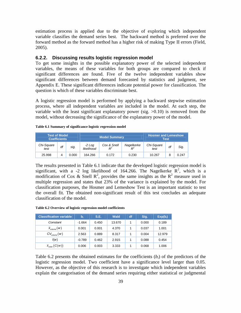
39
estimation process is applied due to the objective of exploring which independent
variable classifies the demand series best. The backward method is preferred over the
forward method as the forward method has a higher risk of making Type II errors (Field,
2005).
6.2.2. Discussing results logistic regression model To get some insights in the possible explanatory power of the selected independent
variables, the means of these variables for both groups are compared to check if
significant differences are found. Five of the twelve independent variables show
significant differences between demand forecasted by statistics and judgment, see
Appendix E. These significant differences indicate potential power for classification. The
question is which of these variables discriminate best.
A logistic regression model is performed by applying a backward stepwise estimation
process, where all independent variables are included in the model. At each step, the
variable with the least significant explanatory power (sig. >0.10) is removed from the
model, without decreasing the significance of the explanatory power of the model.
Table 6.1 Summary of significance logistic regression model
Test of Model Coefficients
Model Summary Hosmer and Lemeshow
Test
Chi-Square test
df sig. -2 Log
likelihood Cox & Snell
R2
Nagelkerke R
2 Chi-Square
test df Sig.
25.998 4 0.000 164.266 0.172 0.230 10.267 8 0.247
The results presented in Table 6.1 indicate that the developed logistic regression model is
significant, with a -2 log likelihood of 164.266. The Nagelkerke R2, which is a
modification of Cox & Snell R2, provides the same insights as the R
2 measure used in
multiple regression and states that 23% of the variance is explained by the model. For
classification purposes, the Hosmer and Lemeshow Test is an important statistic to test
the overall fit. The obtained non-significant result of this test concludes an adequate
classification of the model.
Table 6.2 Overview of logistic regression model coefficients
Classification variable bi S.E. Wald df Sig. Exp(bi)
Constant -1.664 0.450 13.670 1 0.000 0.189
volumex w 0.001 0.001 4.370 1 0.037 1.001
volumeCV w 2.563 0.889 8.317 1 0.004 12.979
( )I w -0.789 0.462 2.915 1 0.088 0.454
orderx C w 0.006 0.003 3.333 1 0.068 1.006
Table 6.2 presents the obtained estimates for the coefficients (bi) of the predictors of the
logistic regression model. Two coefficient have a significance level larger than 0.05.
However, as the objective of this research is to investigate which independent variables
explain the categorisation of the demand series requiring either statistical or judgmental
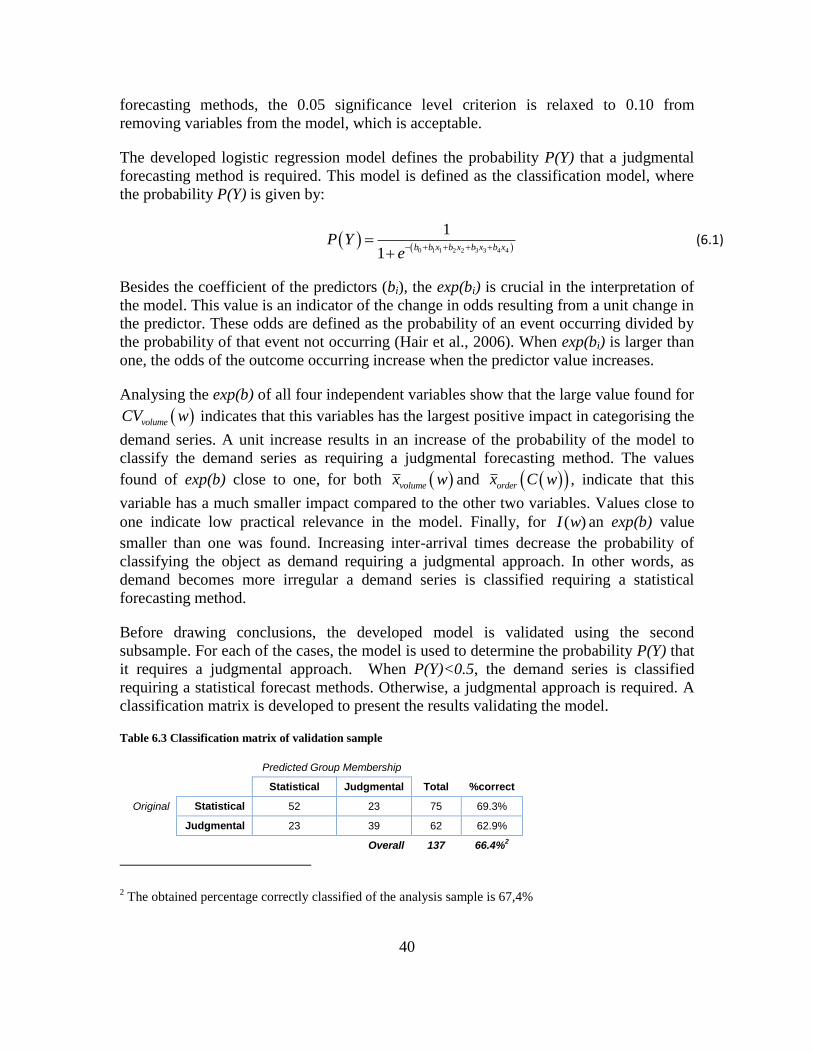
40
forecasting methods, the 0.05 significance level criterion is relaxed to 0.10 from
removing variables from the model, which is acceptable.
The developed logistic regression model defines the probability P(Y) that a judgmental
forecasting method is required. This model is defined as the classification model, where
the probability P(Y) is given by:
0 1 1 2 2 3 3 4 4
1
1b b x b x b x b x
P Ye
(6.1)
Besides the coefficient of the predictors (bi), the exp(bi) is crucial in the interpretation of
the model. This value is an indicator of the change in odds resulting from a unit change in
the predictor. These odds are defined as the probability of an event occurring divided by
the probability of that event not occurring (Hair et al., 2006). When exp(bi) is larger than
one, the odds of the outcome occurring increase when the predictor value increases.
Analysing the exp(b) of all four independent variables show that the large value found for
volumeCV w indicates that this variables has the largest positive impact in categorising the
demand series. A unit increase results in an increase of the probability of the model to
classify the demand series as requiring a judgmental forecasting method. The values
found of exp(b) close to one, for both volumex w and orderx C w , indicate that this
variable has a much smaller impact compared to the other two variables. Values close to
one indicate low practical relevance in the model. Finally, for ( )I w an exp(b) value
smaller than one was found. Increasing inter-arrival times decrease the probability of
classifying the object as demand requiring a judgmental approach. In other words, as
demand becomes more irregular a demand series is classified requiring a statistical
forecasting method.
Before drawing conclusions, the developed model is validated using the second
subsample. For each of the cases, the model is used to determine the probability P(Y) that
it requires a judgmental approach. When P(Y)<0.5, the demand series is classified
requiring a statistical forecast methods. Otherwise, a judgmental approach is required. A
classification matrix is developed to present the results validating the model.
Table 6.3 Classification matrix of validation sample
Predicted Group Membership
Statistical Judgmental Total %correct
Original Statistical 52 23 75 69.3%
Judgmental 23 39 62 62.9%
Overall 137 66.4%
2
2 The obtained percentage correctly classified of the analysis sample is 67,4%
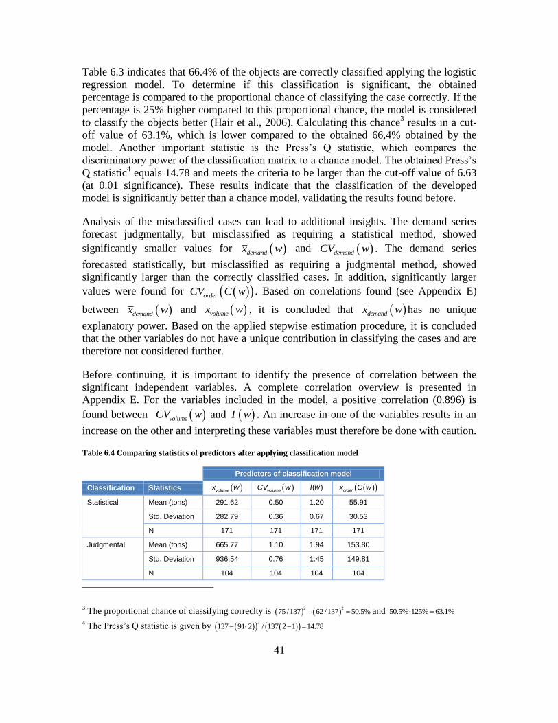
41
Table 6.3 indicates that 66.4% of the objects are correctly classified applying the logistic
regression model. To determine if this classification is significant, the obtained
percentage is compared to the proportional chance of classifying the case correctly. If the
percentage is 25% higher compared to this proportional chance, the model is considered
to classify the objects better (Hair et al., 2006). Calculating this chance3 results in a cut-
off value of 63.1%, which is lower compared to the obtained 66,4% obtained by the
model. Another important statistic is the Press‟s Q statistic, which compares the
discriminatory power of the classification matrix to a chance model. The obtained Press‟s
Q statistic4 equals 14.78 and meets the criteria to be larger than the cut-off value of 6.63
(at 0.01 significance). These results indicate that the classification of the developed
model is significantly better than a chance model, validating the results found before.
Analysis of the misclassified cases can lead to additional insights. The demand series
forecast judgmentally, but misclassified as requiring a statistical method, showed
significantly smaller values for demandx w and demandCV w . The demand series
forecasted statistically, but misclassified as requiring a judgmental method, showed
significantly larger than the correctly classified cases. In addition, significantly larger
values were found for orderCV C w . Based on correlations found (see Appendix E)
between demandx w and volumex w , it is concluded that demandx w has no unique
explanatory power. Based on the applied stepwise estimation procedure, it is concluded
that the other variables do not have a unique contribution in classifying the cases and are
therefore not considered further.
Before continuing, it is important to identify the presence of correlation between the
significant independent variables. A complete correlation overview is presented in
Appendix E. For the variables included in the model, a positive correlation (0.896) is
found between volumeCV w and I w . An increase in one of the variables results in an
increase on the other and interpreting these variables must therefore be done with caution.
Table 6.4 Comparing statistics of predictors after applying classification model
Predictors of classification model
Classification Statistics volumex w volumeCV w ( )I w orderx C w
Statistical Mean (tons) 291.62 0.50 1.20 55.91
Std. Deviation 282.79 0.36 0.67 30.53
N 171 171 171 171
Judgmental Mean (tons) 665.77 1.10 1.94 153.80
Std. Deviation 936.54 0.76 1.45 149.81
N 104 104 104 104
3 The proportional chance of classifying correclty is
2 275 /137 62 /137 50.5% and 50.5% 125% 63.1%
4 The Press‟s Q statistic is given by
2
137 91 2 / 137 2 1 14.78
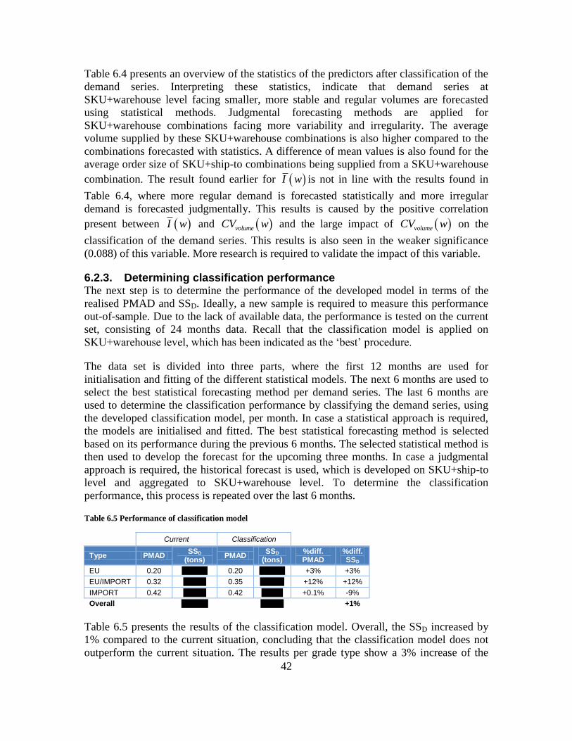
42
Table 6.4 presents an overview of the statistics of the predictors after classification of the
demand series. Interpreting these statistics, indicate that demand series at
SKU+warehouse level facing smaller, more stable and regular volumes are forecasted
using statistical methods. Judgmental forecasting methods are applied for
SKU+warehouse combinations facing more variability and irregularity. The average
volume supplied by these SKU+warehouse combinations is also higher compared to the
combinations forecasted with statistics. A difference of mean values is also found for the
average order size of SKU+ship-to combinations being supplied from a SKU+warehouse
combination. The result found earlier for I w is not in line with the results found in
Table 6.4, where more regular demand is forecasted statistically and more irregular
demand is forecasted judgmentally. This results is caused by the positive correlation
present between I w and volumeCV w and the large impact of volumeCV w on the
classification of the demand series. This results is also seen in the weaker significance
(0.088) of this variable. More research is required to validate the impact of this variable.
6.2.3. Determining classification performance The next step is to determine the performance of the developed model in terms of the
realised PMAD and SSD. Ideally, a new sample is required to measure this performance
out-of-sample. Due to the lack of available data, the performance is tested on the current
set, consisting of 24 months data. Recall that the classification model is applied on
SKU+warehouse level, which has been indicated as the „best‟ procedure.
The data set is divided into three parts, where the first 12 months are used for
initialisation and fitting of the different statistical models. The next 6 months are used to
select the best statistical forecasting method per demand series. The last 6 months are
used to determine the classification performance by classifying the demand series, using
the developed classification model, per month. In case a statistical approach is required,
the models are initialised and fitted. The best statistical forecasting method is selected
based on its performance during the previous 6 months. The selected statistical method is
then used to develop the forecast for the upcoming three months. In case a judgmental
approach is required, the historical forecast is used, which is developed on SKU+ship-to
level and aggregated to SKU+warehouse level. To determine the classification
performance, this process is repeated over the last 6 months.
Table 6.5 Performance of classification model
Current Classification
Type PMAD SSD
(tons) PMAD
SSD (tons)
%diff. PMAD
%diff. SSD
EU 0.20 '''''''''''''''''' 0.20 '''''''''''''''''' +3% +3%
EU/IMPORT 0.32 '''''''''''''''' 0.35 ''''''''''''''''' +12% +12%
IMPORT 0.42 '''''''''''''''' 0.42 ''''''''''''''' +0.1% -9%
Overall
'''''''''''''''
'''''''''''''
+1%
Table 6.5 presents the results of the classification model. Overall, the SSD increased by
1% compared to the current situation, concluding that the classification model does not
outperform the current situation. The results per grade type show a 3% increase of the
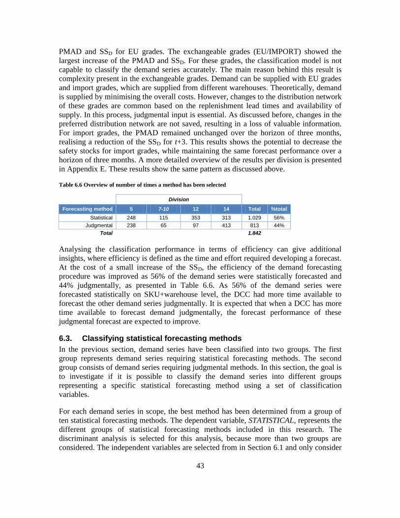
43
PMAD and SSD for EU grades. The exchangeable grades (EU/IMPORT) showed the
largest increase of the PMAD and SSD. For these grades, the classification model is not
capable to classify the demand series accurately. The main reason behind this result is
complexity present in the exchangeable grades. Demand can be supplied with EU grades
and import grades, which are supplied from different warehouses. Theoretically, demand
is supplied by minimising the overall costs. However, changes to the distribution network
of these grades are common based on the replenishment lead times and availability of
supply. In this process, judgmental input is essential. As discussed before, changes in the
preferred distribution network are not saved, resulting in a loss of valuable information.
For import grades, the PMAD remained unchanged over the horizon of three months,
realising a reduction of the SSD for t+3. This results shows the potential to decrease the
safety stocks for import grades, while maintaining the same forecast performance over a
horizon of three months. A more detailed overview of the results per division is presented
in Appendix E. These results show the same pattern as discussed above.
Table 6.6 Overview of number of times a method has been selected
Division
Forecasting method 5 7-10 12 14 Total %total
Statistical 248 115 353 313 1.029 56%
Judgmental 238 65 97 413 813 44%
Total
1.842
Analysing the classification performance in terms of efficiency can give additional
insights, where efficiency is defined as the time and effort required developing a forecast.
At the cost of a small increase of the SSD, the efficiency of the demand forecasting
procedure was improved as 56% of the demand series were statistically forecasted and
44% judgmentally, as presented in Table 6.6. As 56% of the demand series were
forecasted statistically on SKU+warehouse level, the DCC had more time available to
forecast the other demand series judgmentally. It is expected that when a DCC has more
time available to forecast demand judgmentally, the forecast performance of these
judgmental forecast are expected to improve.
6.3. Classifying statistical forecasting methods
In the previous section, demand series have been classified into two groups. The first
group represents demand series requiring statistical forecasting methods. The second
group consists of demand series requiring judgmental methods. In this section, the goal is
to investigate if it is possible to classify the demand series into different groups
representing a specific statistical forecasting method using a set of classification
variables.
For each demand series in scope, the best method has been determined from a group of
ten statistical forecasting methods. The dependent variable, STATISTICAL, represents the
different groups of statistical forecasting methods included in this research. The
discriminant analysis is selected for this analysis, because more than two groups are
considered. The independent variables are selected from in Section 6.1 and only consider
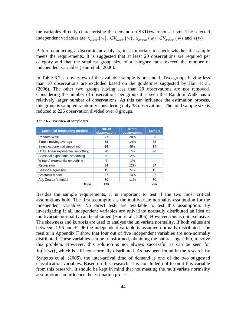
44
the variables directly characterising the demand on SKU+warehouse level. The selected
independent variables are volumex w , volumeCV w , demandx w , demandCV w and ( )I w .
Before conducting a discriminant analysis, it is important to check whether the sample
meets the requirements. It is suggested that at least 20 observations are required per
category and that the smallest group size of a category must exceed the number of
independent variables (Hair et al., 2006).
In Table 6.7, an overview of the available sample is presented. Two groups having less
than 10 observations are excluded based on the guidelines suggested by Hair et al.
(2006). The other two groups having less than 20 observations are not removed.
Considering the number of observations per group it is seen that Random Walk has a
relatively larger number of observations. As this can influence the estimation process,
this group is sampled randomly considering only 38 observations. The total sample size is
reduced to 226 observation divided over 8 groups.
Table 6.7 Overview of sample size
Statistical forecasting method No. of
observations %total
observations Sample
Random Walk 77 28% 38
Simple moving average 38 14% 38
Single exponential smoothing 14 5% 14
Holt’s linear exponential smoothing 20 7% 20
Seasonal exponential smoothing 6 2% -
Winters’ exponential smoothing 4 1% -
Regression 34 12% 34
Season Regression 15 5% 15
Croston’s model 37 13% 37
Adj. Croston’s model 30 11% 30
Total 275
226
Besides the sample requirements, it is important to test if the two most critical
assumptions hold. The first assumption is the multivariate normality assumption for the
independent variables. No direct tests are available to test this assumption. By
investigating if all independent variables are univariate normally distributed an idea of
multivariate normality can be obtained (Hair et al., 2006). However, this is not exclusive.
The skewness and kurtosis are used to analyse the univariate normality. If both values are
between -1.96 and +1.96 the independent variable is assumed normally distributed. The
results in Appendix F show that four out of five independent variables are non-normally
distributed. These variables can be transformed, obtaining the natural logarithm, to solve
this problem. However, this solution is not always successful as can be seen for
ln ( )w , which is still non-normally distributed. As has been found in the research by
Syntetos et al. (2005), the inter-arrival time of demand is one of the two suggested
classification variables. Based on this research, it is concluded not to omit this variable
from this research. It should be kept in mind that not meeting the multivariate normality
assumption can influence the estimation process.
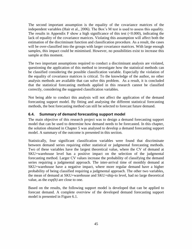
45
The second important assumption is the equality of the covariance matrices of the
independent variables (Hair et al., 2006). The Box‟s M test is used to assess this equality.
The results in Appendix F show a high significance of this test (<0.000), indicating the
lack of equality of the covariance matrices. Violating this assumption will affect both the
estimation of the discriminant function and classification procedure. As a result, the cases
will be over-classified into the groups with larger covariance matrices. With large enough
samples, this impact could be minimised. However, no possibilities exist to increase this
sample at this moment.
The two important assumptions required to conduct a discriminant analysis are violated,
questioning the application of this method to investigate how the statistical methods can
be classified considering the possible classification variable. Especially the violation of
the equality of covariance matrices is critical. To the knowledge of the author, no other
analysis methods are available that can solve this problem. As a result, it is concluded
that the statistical forecasting methods applied in this research cannot be classified
correctly, considering the suggested classification variables.
Not being able to conduct this analysis will not affect the application of the demand
forecasting support model. By fitting and analysing the different statistical forecasting
methods, the best forecasting method can still be selected to forecast future demand.
6.4. Summary of demand forecasting support model
The main objective of this research project was to design a demand forecasting support
model that can be used to determine how demand needs to be forecasted. In this chapter,
the solution obtained in Chapter 5 was analysed to develop a demand forecasting support
model. A summary of the outcome is presented in this section.
Statistically, four significant classification variables were found that discriminate
between demand series requiring either statistical or judgmental forecasting methods.
Two of these variables have the largest theoretical value, where the CV of demand at
SKU+warehouse level has a positive impact on the selection of the judgmental
forecasting method. Larger CV values increase the probability of classifying the demand
series requiring a judgmental approach. The inter-arrival time of monthly demand at
SKU+warehouse have a negative impact, where more regular demand have a higher
probability of being classified requiring a judgmental approach. The other two variables,
the mean of demand at SKU+warehouse and SKU+ship-to level, had no large theoretical
value, as the exp(b) are close to one.
Based on the results, the following support model is developed that can be applied to
forecast demand. A complete overview of the developed demand forecasting support
model is presented in Figure 6.1.
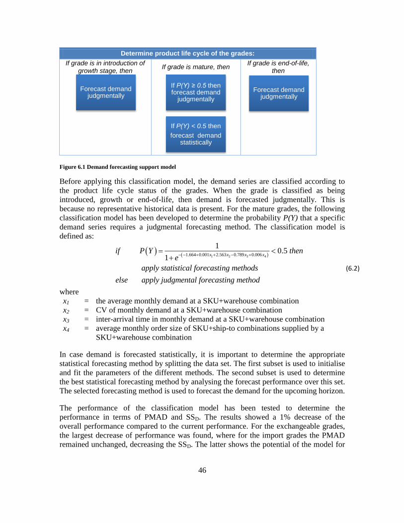
46
Determine product life cycle of the grades:
If grade is in introduction of growth stage, then
If grade is mature, then If grade is end-of-life,
then
Figure 6.1 Demand forecasting support model
Before applying this classification model, the demand series are classified according to
the product life cycle status of the grades. When the grade is classified as being
introduced, growth or end-of-life, then demand is forecasted judgmentally. This is
because no representative historical data is present. For the mature grades, the following
classification model has been developed to determine the probability P(Y) that a specific
demand series requires a judgmental forecasting method. The classification model is
defined as:
1 2 3 41.664 0.001 2.563 0.789 0.006
10.5
1x x x x
if P Y thene
apply statistical forecasting methods
else apply judgmental forecasting method
(6.2)
where
x1 = the average monthly demand at a SKU+warehouse combination
x2 = CV of monthly demand at a SKU+warehouse combination
x3 = inter-arrival time in monthly demand at a SKU+warehouse combination
x4 = average monthly order size of SKU+ship-to combinations supplied by a
SKU+warehouse combination
In case demand is forecasted statistically, it is important to determine the appropriate
statistical forecasting method by splitting the data set. The first subset is used to initialise
and fit the parameters of the different methods. The second subset is used to determine
the best statistical forecasting method by analysing the forecast performance over this set.
The selected forecasting method is used to forecast the demand for the upcoming horizon.
The performance of the classification model has been tested to determine the
performance in terms of PMAD and SSD. The results showed a 1% decrease of the
overall performance compared to the current performance. For the exchangeable grades,
the largest decrease of performance was found, where for the import grades the PMAD
remained unchanged, decreasing the SSD. The latter shows the potential of the model for
Forecast demand judgmentally
If P(Y) ≥ 0.5 then forecast demand
judgmentally
If P(Y) < 0.5 then
forecast demand statistically
Forecast demand judgmentally
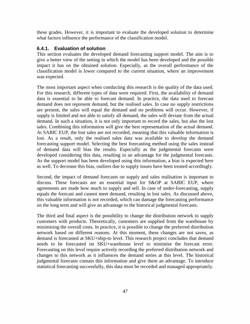
47
these grades. However, it is important to evaluate the developed solution to determine
what factors influence the performance of the classification model.
6.4.1. Evaluation of solution This section evaluates the developed demand forecasting support model. The aim is to
give a better view of the setting in which the model has been developed and the possible
impact it has on the obtained solution. Especially, as the overall performance of the
classification model is lower compared to the current situation, where an improvement
was expected.
The most important aspect when conducting this research is the quality of the data used.
For this research, different types of data were required. First, the availability of demand
data is essential to be able to forecast demand. In practice, the data used to forecast
demand does not represent demand, but the realised sales. In case no supply restrictions
are present, the sales will equal the demand and no problems will occur. However, if
supply is limited and not able to satisfy all demand, the sales will deviate from the actual
demand. In such a situation, it is not only important to record the sales, but also the lost
sales. Combining this information will give the best representation of the actual demand.
At SABIC EUP, the lost sales are not recorded, meaning that this valuable information is
lost. As a result, only the realised sales data was available to develop the demand
forecasting support model. Selecting the best forecasting method using the sales instead
of demand data will bias the results. Especially as the judgmental forecasts were
developed considering this data, resulting in an advantage for the judgmental forecasts.
As the support model has been developed using this information, a bias is expected here
as well. To decrease this bias, outliers due to supply issues have been treated accordingly.
Second, the impact of demand forecasts on supply and sales realisation is important to
discuss. These forecasts are an essential input for S&OP at SABIC EUP, where
agreements are made how much to supply and sell. In case of under-forecasting, supply
equals the forecast and cannot meet demand, resulting in lost sales. As discussed above,
this valuable information is not recorded, which can damage the forecasting performance
on the long term and will give an advantage to the historical judgmental forecasts.
The third and final aspect is the possibility to change the distribution network to supply
customers with products. Theoretically, customers are supplied from the warehouse by
minimising the overall costs. In practice, it is possible to change the preferred distribution
network based on different reasons. At this moment, these changes are not saves, as
demand is forecasted at SKU+ship-to level. This research project concludes that demand
needs to be forecasted on SKU+warehouse level to minimise the forecast error.
Forecasting on this level require actively recording the preferred distribution network and
changes to this network as it influences the demand series at this level. The historical
judgmental forecasts contain this information and give them an advantage. To introduce
statistical forecasting successfully, this data must be recorded and managed appropriately.
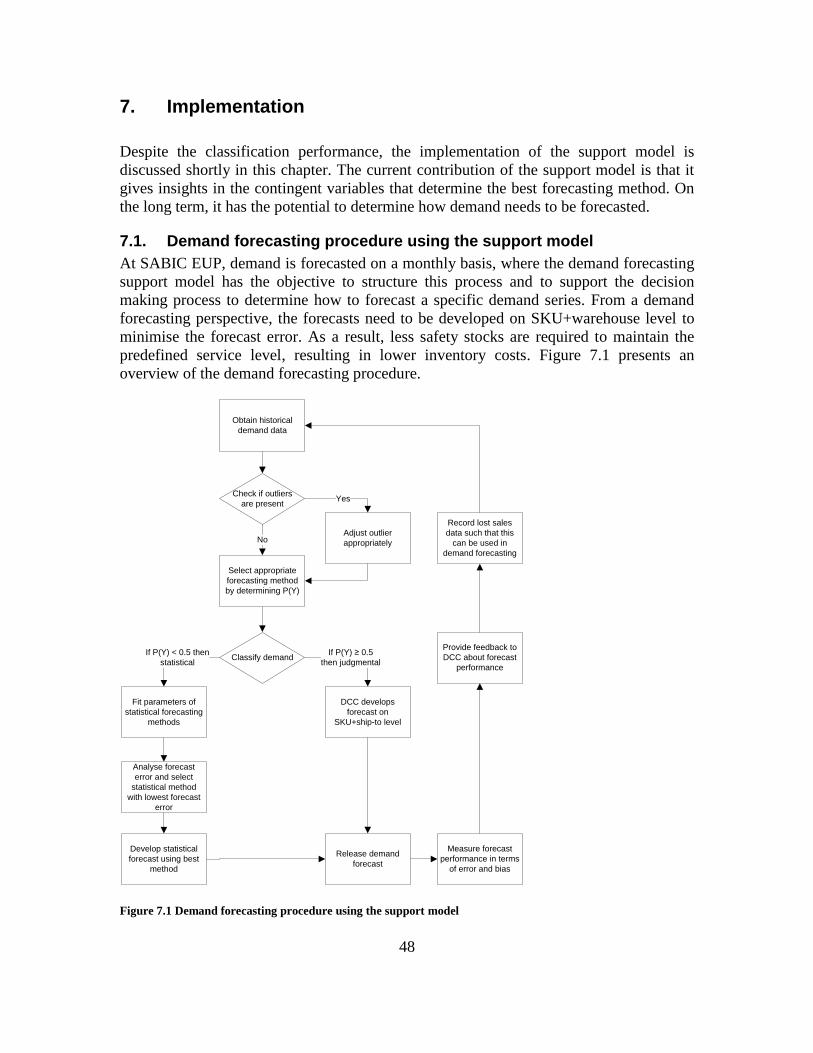
48
7. Implementation
Despite the classification performance, the implementation of the support model is
discussed shortly in this chapter. The current contribution of the support model is that it
gives insights in the contingent variables that determine the best forecasting method. On
the long term, it has the potential to determine how demand needs to be forecasted.
7.1. Demand forecasting procedure using the support model
At SABIC EUP, demand is forecasted on a monthly basis, where the demand forecasting
support model has the objective to structure this process and to support the decision
making process to determine how to forecast a specific demand series. From a demand
forecasting perspective, the forecasts need to be developed on SKU+warehouse level to
minimise the forecast error. As a result, less safety stocks are required to maintain the
predefined service level, resulting in lower inventory costs. Figure 7.1 presents an
overview of the demand forecasting procedure.
Obtain historical
demand data
Check if outliers
are present
Adjust outlier
appropriately
Yes
Select appropriate
forecasting method
by determining P(Y)
No
Classify demandIf P(Y) ≥ 0.5
then judgmental
If P(Y) < 0.5 then
statistical
DCC develops
forecast on
SKU+ship-to level
Fit parameters of
statistical forecasting
methods
Develop statistical
forecast using best
method
Release demand
forecast
Measure forecast
performance in terms
of error and bias
Provide feedback to
DCC about forecast
performance
Record lost sales
data such that this
can be used in
demand forecasting
Analyse forecast
error and select
statistical method
with lowest forecast
error
Figure 7.1 Demand forecasting procedure using the support model
49
The first step of the demand forecasting procedure is to obtain the historical demand data
and to check if outliers are present. These outliers need to be treated accordingly, as has
been suggested by DeLurgio (1998).
The next step is to select the appropriate forecasting method. As discussed before, grades
classified by Business Management as introduction, growth or end-of-life products are
forecasted judgmentally, due to the lack of representative historical demand data. The
mature grades are classified using the developed categorisation model, defining them as
demand requiring statistical or judgmental forecasting methods. In case demand needs to
be forecasted judgmentally, the DCC forecasts the demand on SKU+ship-to level and
these forecasts are aggregated to the required SKU+warehouse level. When a statistical
forecasting method is required, the best method needs to be determined as discussed in
Section 6.4. After selecting the appropriate forecasting method, the statistical forecast is
developed. Once all demand is forecasted, it is released to other internal processes at
SABIC EUP.
The forecast cycle does not end when the forecasts are developed. The next important
step is to measure and analyse the forecast performance in terms of the realised error and
bias. Currently, the latter is not measured, which results in a loss of important
information, because it gives insight if systematic forecast errors are present. A complete
overview of the forecast performance is critical to give the DCCs valuable feedback and
to steer the procedure such that the performance can be improved. In case lost sales occur
due to supply or other issues, it is important to collect this data to acquire a data set
representing the demand and not realised sales.
At SABIC EUP, the SAP R/3 software package is used for enterprise resource planning
(ERP). The SAP Advanced Planner and Optimizer (SAP APO) is a module of SAP R/3,
which is used for demand forecasting. SAP APO is capable to detect outliers and to select
the appropriate statistical forecasting method. At this moment, no bottlenecks are found
that make an integration of the demand forecasting support model impossible. However,
more research in the capability of SAP APO is required before integrating the demand
forecasting support model into SAP APO.
Further, the procedure defined in Figure 7.1 applies the categorisation model and
determines the best forecasting methods every cycle. Instead, it would be interesting to
investigate if tracking signals can be applied to monitor the performance of the developed
forecasts to determine if they need to be reclassified to determine the best forecasting
methods. This would be an interesting area of future research.
50
8. Conclusion and recommendations
8.1. Conclusions
The objective of this research was to develop a demand forecasting support model for a
process industry company selling commodity products, like SABIC EUP. This model
gives insights in the contingent variables of forecasting and determine the appropriate
method to forecast demand. To develop such a support model, two research questions
were developed.
What is the best procedure to develop the demand forecast for SABIC EUP?
The objective of demand forecasting is to develop forecasts that minimise the forecast
error on SKU+warehouse level, as this is the position of the CODP. This research project
concluded that forecasts developed at this level realised this objective, applying both
statistical and judgmental forecasting methods. Selecting the best forecasting method per
demand series results in a reduction of the forecast error (PMAD), resulting in a decrease
in safety stocks (SSD), required to cover the demand variability of 17% compared to the
current performance. This reduction in SSD indicated a potential saving realised by
selecting the best forecast method. Assuming a cost price of 1.1 k€ per ton and a WACC
of 12% of the cost price per year, a 12.6 kton reduction of the SSD decreases the costs by
1,658 k€ per year for SABIC EUP.
In practice, this saving is difficult to realise, as it is not possible to determine upfront if
statistical or judgmental forecasting methods are required. To find a solution for this
problem, a demand forecasting support model is developed by answering the second
research question.
How can the results, obtained from the previous research question, be transformed into a
general model that determines the most appropriate forecasting method, taking into
consideration the demand characteristics?
The primary objective of the demand forecasting support model is to determine if a
demand series requires a statistical or a judgmental method to forecast demand. First, the
grades were classified considering their product life cycle status. The grades classified in
the introduction, growth and end-of-life product life cycle stage are forecasted using the
judgmental method due to the lack of representative historical demand data. For the
mature grades, the results obtained from the first research question are used to develop a
classification model that determines how to forecast demand for these grades.
The developed classification model is a logistic regression model determining the
probability P(Y) that a judgmental forecasting approach is required. Analysing the
significant predictors in the model, the following is concluded:
- The CV of the monthly demand on SKU+warehouse level has the largest impact
on classification of the demand series. Larger CVs increase the probability that a
judgmental method is required
51
- The inter-arrival time of monthly demand on SKU+warehouse level has a
negative impact on the probability of selecting a judgmental forecasting method.
More irregular demand is has a higher probability of being classified requiring
statistical forecasting methods. Due to the correlation found between this variable
and the previous variable, this result should be interpreted with caution and more
research is required to validate this results.
- Both the average monthly demand at SKU+warehouse level and the average
monthly order size at SKU+ship-to level are also included in the classification
model. However, these variables have limited practical relevance as their impact
is very small.
This research project also investigated the possibility to categorise the statistical
forecasting methods. However, due to the violations of critical assumptions of the
method, no classification model could be developed.
In case a statistical forecasting method is required, it is important to select the appropriate
method by splitting the demand history. The first subset is used to initialise and fit the
parameters of the models and the second subset is used to analyse the forecast
performance. The best statistical forecasting method is selected based on the performance
over this second subset.
The performance of the classification model was also determined in terms of the PMAD
and SSD. The results indicated a small decrease of the overall forecasting performance
(+1%) and concluded that the model, despite of its statistical significant classification
performance, was not able to realise the potential 17% improvement when applied in
forecasting.
Different reasons have been discussed that could explain the large deviation between the
potential improvement and actual performance. A summary is presented in the next
section as recommendation to SABIC EUP. These issues need to be addressed to improve
the performance of the classification model, as it is assumed that these issues have a
significant impact on the performance.
8.2. Recommendations to SABIC EUP
Save both initial forecast developed before S&OP and agreed forecast after S&OP
In demand forecasting, it is essential to record data that give insights in the expected and
actual demand. The initial demand forecast can be adjusted based on information
discussed during S&OP, resulting in an agreed forecast. Not recording these changes will
result in a loss of valuable information, affecting future demand forecasts. To enable
future research, recording this information is important.
Record lost sales and extreme events
In demand forecasting, the data used should represent the actual demand. In practice, the
data used only represents the realised sales. In situations where all demand is satisfied, no
deviations will occur. When, due to circumstances, not all demand can be satisfied, it is
important to record the sales lost. This valuable lost sales data in combination with the
52
realised sales data gives a better representation of the actual demand. Collecting this data
will minimise the bias from the actual demand, resulting in increased data quality and
forecasting performance.
Record changes in distribution network
This research concluded that minimising the forecast error at SKU+warehouse level
requires the development of the demand forecasts at this level as well. Currently,
customers are supplied from preferred warehouses by minimising the overall costs.
However, changes are applied due to several reasons. As demand is forecasted at
warehouse level, it is essential to record these changes to create reliable data,
representing the actual realisation.
Conduct a pilot before implementing the support model
To get a complete overview of the impact on the supply chain of SABIC EUP, a pilot is
suggested. This pilot must be conducted parallel to the current procedure, enabling a
better comparison of both procedures. Bottlenecks of the new demand forecasting support
model can also be identified and can be solved accordingly.
Control demand forecasting performance
Besides measuring the forecast error, it is important to measure the forecast bias to check
if systematic errors are present. Monitoring performance and providing feedback to the
DCC is essential for controlling the demand forecasting performance and for creating an
environment of continuous improvements.
Differentiate the demand forecasting for different planning horizons
In this research project, a demand forecasting support model has been developed for
short-term tactical planning. Other important planning horizons are the mid-term and
long-term planning, used for (mid-term) tactical and (long-term) strategic decision
processes. For SABIC EUP, the different horizons have different objective, which need
to be considered in forecasting. To fit these objective optimally, differentiation of the
procedure is required for the different planning horizons.
Investigate differentiation of distribution capacity planning from demand planning
The current practice of demand forecasting is to forecast demand on SKU+ship-to level
such that both demand planning and distribution capacity planning are satisfied using
only one forecast. The focus of this research project was on improving demand
forecasting only. This is realised by forecasting on SKU+warehouse level. Providing
distribution capacity information, this forecast is disaggregated to SKU+ship-to level,
resulting in a small decrease in forecast performance at this level. Although this small
decrease is assumed to have limited impact, it is recommended to investigate how
distribution capacity planning could be designed such that the best forecast can be made
for this planning process.
53
8.3. Recommendations for future research
Continue research in the area of demand categorisation
As Makridakis and Hibon (2000) stated, no best performing forecasting method is
available. Since the research on demand categorisation is sparse, it is an interesting area
to conduct research. The first well-developed model by Syntetos et al. (2005), determined
the areas of superior performance analysing four statistical forecasting methods
analytically. This research was not able to determine these areas of superior performance.
Increasing the sample and improving the data quality may increase the probability of
developing such a model empirically.
This research project was successful in providing insights in which variables could
explain the difference between demand series forecasted by statistics and judgment.
However, more research is required to improve the classification performance out-of-
sample. It would be interesting to investigate which variables are currently missing, that
could describe the differences between statistical and judgmental forecasting.
Investigate how price elasticity can be incorporated in demand forecasting
The pricing strategy of the products is considered an important determinant of the actual
demand in a commodity business. This research concluded that price variability did not
had any explanatory power in determining if demand required a judgmental forecasting
method. Discussing this result with the DCCs, indicated that they do not have any
knowledge about the direct impact of price changes on demand. For future research,
investigating this impact of price changes on demand (price elasticity) could lead to
additional insights that can be used to forecast demand. Due to the complex nature of
such models and the large list of possible variables, more research is required in this area.
54
References
1. Bertrand, J.W.M. and Fransoo, J. C., (2002), Operations management research
methodologies using quantitative modelling, International Journal of Operations
& Production Management, Vol. 22 No. 2, pp. 241-264.
2. Boylan, J. E., Syntetos, A. A. and Karakostas, G. C., (2008), Classification for
forecasting and stock control: a case study, Journal of the Operational Research
Society, Vol. 59, pp. 473-481.
3. Chatfield, C. (2000), Time-series forecasting, Florida: Chapman & Hall/CRC.
4. Chen, A. and Blue, J., (2010), Performance analysis of demand planning
approaches for aggregating, forecasting and disaggregating interrelated demands,
International Journal of Production Economics, Vol. 128, pp. 586-602.
5. Danese, P. And Kalchschmidt, M., (2010), The impact of forecasting on
companies‟ performance: Analysis in a multivariate setting, International Journal
of Production Economics, In press.
6. DeLurgio, S. A., (1998), Forecasting Principles and Applications, First edition,
Irwin/McGraw-Hill.
7. Field, A. (2005). Discovering Statistics using SPSS. 2nd
ed. Sage.
8. Fransoo, J. C., (1992), Demand Management and Production Control in Process
Industries, International Journal of Operations & Production Management, Vol.
12, pp. 187-196.
9. Goodwin, P., (2002), Integrating management judgment and statistical methods to
improve short-term forecasts, Omega, Vol. 30, pp. 127-135.
10. Hair, J. F., Black, W. C., Babin, B. J., Anderson, R. E. And Tatham, R. L., (2006),
Multivariate Data Analysis, Sixth edition, Pearson Eduction Inc. New Jersey.
11. Hyndman, R. J. and Koehler, A. B., (2006), Another look at measures of forecast
accuracy, International Journal of Forecast, Vol. 22, pp. 679-688.
12. Jüttner, U., Christopher, M. and Baker, S., (2007), Demand chain management-
integrating marketing and supply chain management, Industrial Marketing
Management, Vol. 36, pp. 377-392.
13. Kleuskens, J., (2011), Demand planning: a literature review, Eindhoven
University of Technology, Literature Review for Master Thesis Preparation
(1LM05).
14. Kok, de, A.G. and Fransoo, J. C., (2003), Chapter 14 in “Supply Chain
Management”, Handbooks in Operations Research and Management Science
series, Amsterdam: North Holland.
15. Makridakis, S. and Hibon, M., (2000), The M3-Competition: results, conclusions
and implications, International Journal of Forecasting, Vol. 16, pp. 451-476.
55
16. Mitroff, I. I., Betz, F., Pondy, L. R. and Sagasti, F., (1974), On managing science
in the systems age: two schemas for the study of science as a whole system
phenomenon, Interfaces, Vol. 4 No. 3, pp. 46-58.
17. Montgomery, D. C., (2009), Design and Analysis of Experiments, 7th edition,
John Wiley & Sons (Asia) Pte Ltd
18. SABIC, “SABIC in Europe”*Online]. 2008; [Cited: January 31, 2011] available
at http://www.sabic-europe.com/_en/.
19. Silver, E. A., Pyke, D. F. and Peterson, R., (1998), Inventory Management and
Production Planning and Scheduling, John Wiley & Sons Inc. New York.
20. Stadler, H. and Kilger, C., (2008), Supply Chain Management and Advanced
Planning; Concepts, Models, Software, and Case Studies, Springer-Verlag Berlin
Heidelberg.
21. Syntetos, A. A., Boylan, J. E. and Croston, J. D., (2005), On the categorization of
demand patterns, The Journal of the Operational Research Society, Vol. 56, No.
5, pp. 495-503.
22. Syntetos, A. A. and Boylan, J. E., (2001), On the bias of intermittent demand
estimates, International Journal of Production Economics, Vol. 71, pp. 457-466.
23. Widiarta, H., Viswanathan, S. and Piplani, R., (2008), Forecasting item-level
demands: an analytical evaluation of top-down versus bottom-up forecasting in a
production-planning framework, IMA Journal of Management Mathematics, Vol.
19, pp. 207-218.
24. Zotteri, G., Kalchschmidt, M. and Caniato, F., (2005), The impact of aggregation
level on forecasting performance, International Journal of Production Economics,
Vol. 93-94, pp. 479-491.
25. Zotteri, G. and Kalchschmidt, M., (2007), A model for selecting the appropriate
level of aggregation in forecasting processes, International Journal of Production
Economics, Vol. 108, pp. 74-83.
56
Glossary of terms
BU Business Unit, representing a product group
CIT Container-In-Transit
DCC Demand Chain Coordinator, who is responsible for demand planning
DS Detailed Schedule
EU grades Grades that are exclusively produced in Europe
EU/IMPORT grades Exchangeable grades which can be produced in Europe or can be
imported from KSA
Grade A subtype of a product, characterised by a unique set of chemical
properties
Import grades Grades that are exclusively imported from KSA
KSA Kingdom of Saudi Arabia
MPS Master Production Schedule
MTS Make To Stock
PMAD Percentage Mean Absolute Deviation
S&OP Sales & Operations Planning
SABIC Saudi Basic Industries Corporation
SABIC EUP SABIC Europe SBU Polymers
SBU Strategic Business Unit
Ship-to Customer location where goods can be delivered
SIM Supply and Inventory Manager
SKU Stock Keeping Unit
SKU+ship-to A unique customer ordering a specific SKU
SKU+warehouse A SKU delivered from a specific warehouse
SNP Supply Network Planning
SPR Sales Plan Realisation
SSD Safety stock required to cover for the demand variability and
maintaining the predefined service level
VT Value Team, representing a group of grades serving a specific
business
WACC Weighted Average Cost of Capital
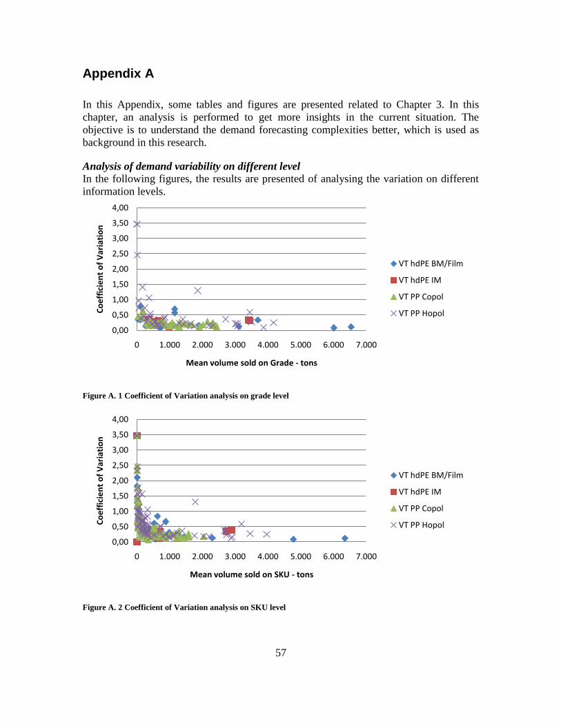
57
Appendix A
In this Appendix, some tables and figures are presented related to Chapter 3. In this
chapter, an analysis is performed to get more insights in the current situation. The
objective is to understand the demand forecasting complexities better, which is used as
background in this research.
Analysis of demand variability on different level
In the following figures, the results are presented of analysing the variation on different
information levels.
Figure A. 1 Coefficient of Variation analysis on grade level
Figure A. 2 Coefficient of Variation analysis on SKU level
0,00
0,50
1,00
1,50
2,00
2,50
3,00
3,50
4,00
0 1.000 2.000 3.000 4.000 5.000 6.000 7.000
Co
eff
icie
nt
of
Var
iati
on
Mean volume sold on Grade - tons
VT hdPE BM/Film
VT hdPE IM
VT PP Copol
VT PP Hopol
0,00
0,50
1,00
1,50
2,00
2,50
3,00
3,50
4,00
0 1.000 2.000 3.000 4.000 5.000 6.000 7.000
Co
eff
icie
nt
of
Var
iati
on
Mean volume sold on SKU - tons
VT hdPE BM/Film
VT hdPE IM
VT PP Copol
VT PP Hopol
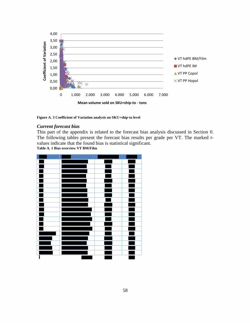
58
Figure A. 3 Coefficient of Variation analysis on SKU+ship-to level
Current forecast bias
This part of the appendix is related to the forecast bias analysis discussed in Section 0.
The following tables present the forecast bias results per grade per VT. The marked t-
values indicate that the found bias is statistical significant. Table A. 1 Bias overview VT BM/Film
'''''''''' '''''''''''' ''''''''''''''''' ''''''''' ''''''''''''''
'''''''' ''''''''''''''''' ''''''''''''''' ''''''''''''' ''''''''''''
'''''''' ''''''''''''''' ''''''''''''''' '''''''''' ''''''''''
''''''' ''''''''''''''' '''''''''''''''' ''''''''''' '''''''''
''''''' ''''''''''''''' '''''''''''''' '''''''''' ''''''''''
''''''' ''''''''''''''' ''''''''''''''' ''''''''''''' '''''''''''
''''''' '''''''''''''' ''''''''''''''' ''''''''''' ''''''''''
''''''' ''''''''''''''' '''''''''''''''' '''''''''''' ''''''''''
''''''' ''''''''''''''' '''''''''''''''' '''''''''''' '''''''''
''''''' '''''''''''''''''' '''''''''''''''' ''''''''' ''''''''
'''''''' ''''''''''''''''''''' '''''''''''''' ''''''''''''' '''''''''''
'''''''' '''''''''''''''''''''''''''''' '''''''''''''' '''''''''''' ''''''''
'''''''' '''''''''''''''''''''''''' ''''''''''''''' ''''''''''' ''''''''''
''''''' ''''''''''''''''''''''''''''' '''''''''''''' '''''''''' ''''''''''
''''''' ''''''''''''''''''''''''' ''''''''''''''' ''''''''''''' ''''''''''
''''''' '''''''''''''''''''''''' ''''''''''''''' ''''''''''' '''''''''
''''''''''''''''''''''''''' '''''''''''''''''''''' ''''''''''''''' ''''''''''' '''''''''
''''''''''''''''''''' '''''''''''''''' '''''''''''''''' ''''''''''''' '''''''''''
''''''''''''''''''' ''''''''''''''' ''''''''''''''' ''''''''''''' ''''''''
''''''''''''''''''''' '''''''''''''''''''' ''''''''''''''' '''''''''''' '''''''''''
'''''''''''''''''''''' ''''''''''''''''' '''''''''''''''' '''''''''''' ''''''''
' '''''''''''''' '''''''''''' ''''''''
0,00
0,50
1,00
1,50
2,00
2,50
3,00
3,50
4,00
0 1.000 2.000 3.000 4.000 5.000 6.000 7.000
Co
eff
icie
nt
of
Var
iati
on
Mean volume sold on SKU+ship-to - tons
VT hdPE BM/Film
VT hdPE IM
VT PP Copol
VT PP Hopol
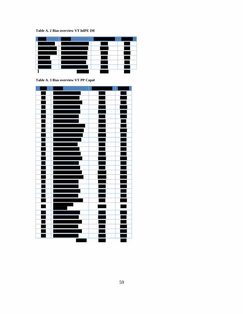
59
Table A. 2 Bias overview VT hdPE IM
''''''''''' ''''''''''''' '''''''''''''''''' ''''''''' '''''''''''''''
'''''''''''''''''''''''''''' '''''''''''''''''''''' ''''''''''''''' '''''''''''' ''''''''
''''''''''''''''''''''''''''''' '''''''''''''''''''' '''''''''''''''' '''''''''''''' ''''''''''
''''''''''''''''''''''''''''''' ''''''''''''''''''''' ''''''''''''''' '''''''''''' '''''''''''
'''''''''''''''''''' '''''''''''''''''''' '''''''''''''''' ''''''''''' ''''''''''
'''''''''''''''''''''' '''''''''''''''''''' '''''''''''''' '''''''''''' '''''''''
'''''''''''''''''''''' ''''''''''''''''''''' '''''''''''''''' '''''''''''' ''''''''
' '''''''''''''''' '''''''''''''' ''''''''
Table A. 3 Bias overview VT PP Copol
''''''''' ''''''''''''' '''''''''''''''''' '''''''' '''''''''''''''
'''''''' ''''''''' ''''''' ''''''' ''''''''''''''' ''''''''''' ''''''''
''''''' '''''''' '''''''' '''''' '''''''''''''' ''''''''''' '''''''''
'''''''' ''''''''' '''''''''''' '''''' ''''''''''''''' ''''''''''' ''''''''''
''''''' '''''''' '''''''' '''''' ''''''''''''''' '''''''''''' ''''''''''''
'''''''' '''''' ''''''''' '''''' ''''''''''''''' ''''''''''''' '''''''''
'''''''' '''''''''''''''' '''''''''''''''' ''''''''''' '''''''''''
''''''' '''''''''''''''' '''''''''''''''' '''''''''''' '''''''''
''''''' '''''''''''''''''''''''''''''' ''''''''''''''''''''' '''''''''''' ''''''''
''''''' ''''''''''''''''''''''''''''' '''''''''''''''''''' '''''''''''' '''''''''
'''''''' ''''''''' '''''''''''' '''''' '''''''''''''''' ''''''''''''' ''''''''''
''''''' ''''''''' '''''''' ''''''' ''''''''''''''' '''''''''''' ''''''''
''''''' ''''' ''''' '''''' '''''''''''''' ''''''''''' ''''''''
'''''''' '''''' ''''' ''''''' ''''''''''''''' ''''''''''' ''''''''
''''''' '''''''' ''''''''' ''''''' '''''''''''''' '''''''''''' ''''''''
'''''''' '''''''' ''''''''''' ''''''' '''''''''''''''' ''''''''''''' '''''''''
''''''' '''''' ''''' ''''' '''''''''''''''' '''''''''''' ''''''''
'''''''' ''''' '''''''''''' ''''' ''''''''''''''' ''''''''''' ''''''''
'''''''' '''''''''' ''''''''' ''''' '''''''''''''''' '''''''''''''' '''''''''''
'''''''' '''''' ''''''' ''''''' '''''''' '''''''''''''''' '''''''''''''' '''''''''
''''''' '''''' ''''''' ''''' ''''''''''''''' ''''''''''''' '''''''''''
''''''' '''''' ''''''' ''''' ''''''''''''''' '''''''''''' '''''''''''
''''''' '''''' ''''''''' '''''' ''''''''''''''' '''''''''''' ''''''''''
''''''' '''''''''''''''' ''''''''''''''' '''''''''''' ''''''''
'''''''' ''''''''''''''''''''''''''''''''''''''''''''''''' ''''''''''' '''''''''
'''''''' ''''''''''''''''''''''''''''''''' '''''''''''''''''''''''
'''''''''''''' ''''''''
'''''''' '''''''''''' '''''' '''''''''''''''' '''''''''''' '''''''''
'''''''' '''''''''''' '''''' '''''''''''''' ''''''''''''' ''''''''
''''''' ''''''''''' ''''''' '''''' '''''''''''''''' '''''''''''' ''''''''
'''''''' ''''''''''' '''''' '''''''''''''' ''''''''''' '''''''''
'''''''' '''''''''''' '''''' '''''' '''''''''''''''' ''''''''''' '''''''''
'''''''' ''''''''''''''''''' '''''''''''''' '''''''''''' '''''''''''
'''''''''''''' '''''''''''' ''''''''

60
Table A. 4 Bias overview VT PP Hopol
'''''''''' ''''''''''''' '''''''''''''''' ''''''''' ''''''''''''''
'''''''''''''''''''''''''''' '''''''''''' '''''''''''''''' '''''''''''' '''''''''
''''''''''''''''''''''''''''''' '''''''''''' ''''''''''''''' '''''''''''''' '''''''''
'''''''' '''''''''''''' '''''''''''''' ''''''''''' '''''''''''
'''''''' '''''''''''' '''''''''''''' '''''''''' ''''''''''
''''''' '''''''''''' ''''''''''''''''' ''''''''''''' ''''''''
''''''' '''''''''''''' ''''''''''''''' '''''''''''' ''''''''''
'''''''' '''''''''''' '''''''''''''''' '''''''''''' '''''''''''
'''''''' '''''''''''' ''''''''''''''' '''''''''''' ''''''''
''''''' '''''''''''' '''''''''''''''' ''''''''''' '''''''''''
'''''''' ''''''''''' ''''''''''''''' ''''''''''' '''''''''''
''''''' '''''''''''' ''''''''''''''' ''''''''''' ''''''''
''''''' ''''''''''''' '''''''''''''' '''''''''''' ''''''''''
''''''' '''''''''''' ''''''''''''''' ''''''''''' ''''''''''
''''''' ''''''''''''' '''''''''''''''' ''''''''''' '''''''''''
'''''''' '''''''''''''' '''''''''''''' ''''''''''''' '''''''''
''''''' ''''''''''''' '''''''''''''''' ''''''''''''' '''''''''
'''''''' ''''''''''''' ''''''''''''''' '''''''''' '''''''''''
''''''' ''''''''''''' '''''''''''''' ''''''''''''' ''''''''
''''''' '''''''''''' ''''''''''''''' '''''''''''''' ''''''''''
'''''''' ''''''''''''' ''''''''''''''''' '''''''''''' ''''''''''
''''''' ''''''''''''' '''''''''''''''' ''''''''''''' '''''''''''
'''''''' '''''''''''''''' ''''''''''''''' ''''''''''''' '''''''''''
'''''''' ''''''''''' ''''''''''''''''' ''''''''''' '''''''''
'''''''' ''''''''''''' '''''''''''''''' ''''''''''''' ''''''''''
'''''''' '''''''''''' '''''' '''''''''''''''' '''''''''''' '''''''''''
''''''' ''''''''''''''''''''' ''''''''''''''''' '''''''''' '''''''''
''''''' '''''''''''''''''''' '''''''''''''''' '''''''''''' ''''''''
''''''' ''''''''''''''''''''' ''''''''''''''' ''''''''''''' '''''''''
''''''' ''''''' '''''' '''''''' '''''' '''''''''''''' ''''''''''' '''''''''
'''''''' ''''''''''' '''' '''''' '''''''''''''' ''''''''''' ''''''''''
'''''''''''''''''''''' '''''''''''' ''''''''''''''' ''''''''''''' '''''''''''
'''''''''''''''''''''' '''''''''''''' '''''''''''''' ''''''''''''' '''''''''
''''''''''''''''''''''' '''''''''''' '''''''''''''''' '''''''''''' '''''''''''
''''''''''''''''''' '''''''''''' '''''''''''''''' '''''''''''' ''''''''
'''''''''''''''''''''' '''''''''''''' '''''''''''''' ''''''''''''' ''''''''''
''''''''''''''''''''' ''''''''''''' '''''''''''''''' '''''''''''' ''''''''''
'''''''''''''''''''''' '''''''''''''' ''''''''''''''' ''''''''''''' '''''''''''
'''''''''''''''''''''' ''''''''''''' ''''''''''''''' '''''''''' ''''''''''''
''''''''''''''''''' '''''''''''''' '''''''''''''' ''''''''''' '''''''''
''''''''''''''''''''''' '''''''''''' '''''''''''''''' '''''''''' ''''''''''''
''''''''''''''''''' '''''''''''''' ''''''''''''''' ''''''''''' '''''''''''
'' '''''''''''''''''' '''''''''''' '''''''''
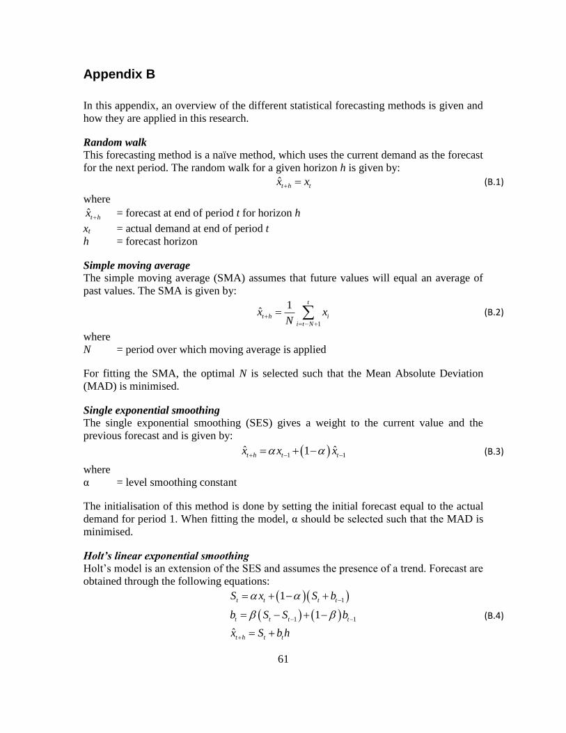
61
Appendix B
In this appendix, an overview of the different statistical forecasting methods is given and
how they are applied in this research.
Random walk
This forecasting method is a naïve method, which uses the current demand as the forecast
for the next period. The random walk for a given horizon h is given by:
ˆt h tx x (B.1)
where
ˆt hx = forecast at end of period t for horizon h
xt = actual demand at end of period t
h = forecast horizon
Simple moving average
The simple moving average (SMA) assumes that future values will equal an average of
past values. The SMA is given by:
1
1ˆ
t
t h i
i t N
x xN
(B.2)
where
N = period over which moving average is applied
For fitting the SMA, the optimal N is selected such that the Mean Absolute Deviation
(MAD) is minimised.
Single exponential smoothing
The single exponential smoothing (SES) gives a weight to the current value and the
previous forecast and is given by:
1 1ˆ ˆ1t h t tx x x (B.3)
where
α = level smoothing constant
The initialisation of this method is done by setting the initial forecast equal to the actual
demand for period 1. When fitting the model, α should be selected such that the MAD is
minimised.
Holt’s linear exponential smoothing
Holt‟s model is an extension of the SES and assumes the presence of a trend. Forecast are
obtained through the following equations:
1
1 1
1
1
ˆ
t t t t
t t t t
t h t t
S x S b
b S S b
x S b h
(B.4)
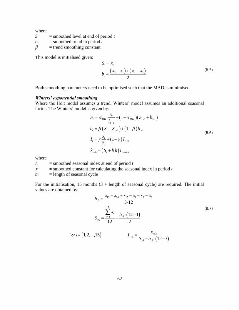
62
where
St = smoothed level at end of period t
bt = smoothed trend in period t
= trend smoothing constant
This model is initialised given:
1 1
2 1 4 3
12
S x
x x x xb
(B.5)
Both smoothing parameters need to be optimised such that the MAD is minimised.
Winters’ exponential smoothing
Where the Holt model assumes a trend, Winters‟ model assumes an additional seasonal
factor. The Winters‟ model is given by:
1 1
1 1
1
1
1
ˆ
tt HW HW t t
t L
t t t t
tt t m
t
t h t t t h m
xS S b
I
b S S b
xI I
S
x S b h I
(B.6)
where
It = smoothed seasonal index at end of period t
= smoothed constant for calculating the seasonal index in period t
m = length of seasonal cycle
For the initialisation, 15 months (3 + length of seasonal cycle) are required. The initial
values are obtained by:
13 14 15 1 2 316
15
16416
3 12
12 1
12 2
t
t
x x x x x xb
xb
S
(B.7)
For i = 1,2,...,15
33
16 16 12
ii
xI
S b i
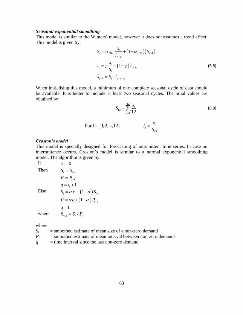
63
Seasonal exponential smoothing
This model is similar to the Winters‟ model, however it does not assumes a trend effect.
This model is given by:
11
1
ˆ
tt HW HW t
t m
tt t m
t
t h t t h m
xS S
I
xI I
S
x S I
(B.8)
When initialising this model, a minimum of one complete seasonal cycle of data should
be available. It is better to include at least two seasonal cycles. The intial values are
obtained by:
12
13
1 12
t
t
xS
(B.9)
For i = 1,2,...,12 13
ii
xI
S
Croston’s model
This model is specially designed for forecasting of intermittent time series. In case no
intermittence occurs, Croston‟s model is similar to a normal exponential smoothing
model. The algorithm is given by:
If 0tx
Then 1
1
1
t t
t t
S S
P P
q q
Else
1
1
1
1
1
t t t
t t
S x S
P q P
q
where ˆ /t h t tx S P
where
St = smoothed estimate of mean size of a non-zero demand
Pt = smoothed estimate of mean interval between non-zero demands
q = time interval since the last non-zero demand
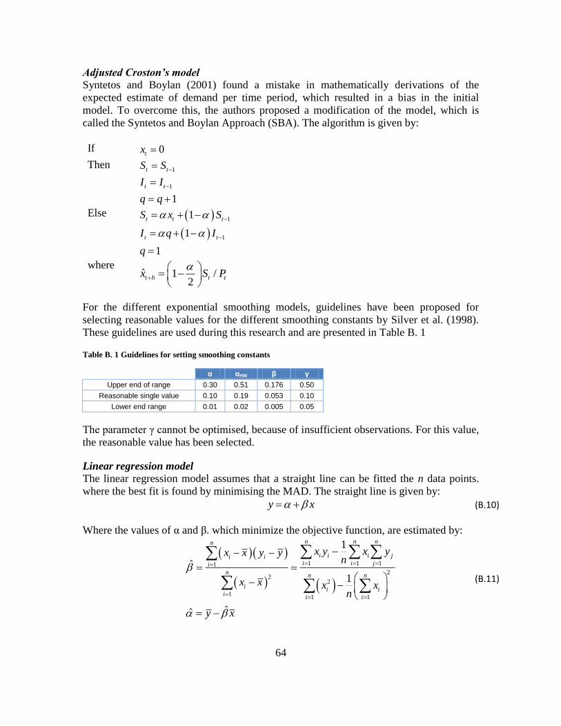
64
Adjusted Croston’s model
Syntetos and Boylan (2001) found a mistake in mathematically derivations of the
expected estimate of demand per time period, which resulted in a bias in the initial
model. To overcome this, the authors proposed a modification of the model, which is
called the Syntetos and Boylan Approach (SBA). The algorithm is given by:
If 0tx
Then 1
1
1
t t
t t
S S
I I
q q
Else
1
1
1
1
1
t t t
t t
S x S
I q I
q
where ˆ 1 /
2t h t tx S P
For the different exponential smoothing models, guidelines have been proposed for
selecting reasonable values for the different smoothing constants by Silver et al. (1998).
These guidelines are used during this research and are presented in Table B. 1
Table B. 1 Guidelines for setting smoothing constants
α αHW β γ
Upper end of range 0.30 0.51 0.176 0.50
Reasonable single value 0.10 0.19 0.053 0.10
Lower end range 0.01 0.02 0.005 0.05
The parameter γ cannot be optimised, because of insufficient observations. For this value,
the reasonable value has been selected.
Linear regression model
The linear regression model assumes that a straight line can be fitted the n data points.
where the best fit is found by minimising the MAD. The straight line is given by:
y x (B.10)
Where the values of α and β. which minimize the objective function, are estimated by:
1 1 11
22
2
11 1
1
ˆ
1
ˆˆ
n n nn
i i i ji ii i ji
nn n
ii i
ii i
x y x yx x y yn
x x x xn
y x
(B.11)
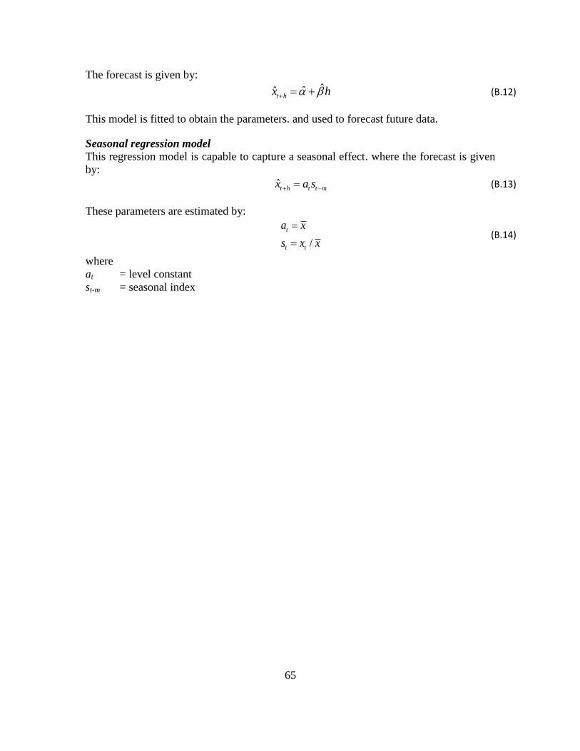
65
The forecast is given by:
ˆˆˆt hx h (B.12)
This model is fitted to obtain the parameters. and used to forecast future data.
Seasonal regression model
This regression model is capable to capture a seasonal effect. where the forecast is given
by:
ˆt h t t mx a s (B.13)
These parameters are estimated by:
/
t
t t
a x
s x x
(B.14)
where
at = level constant
st-m = seasonal index
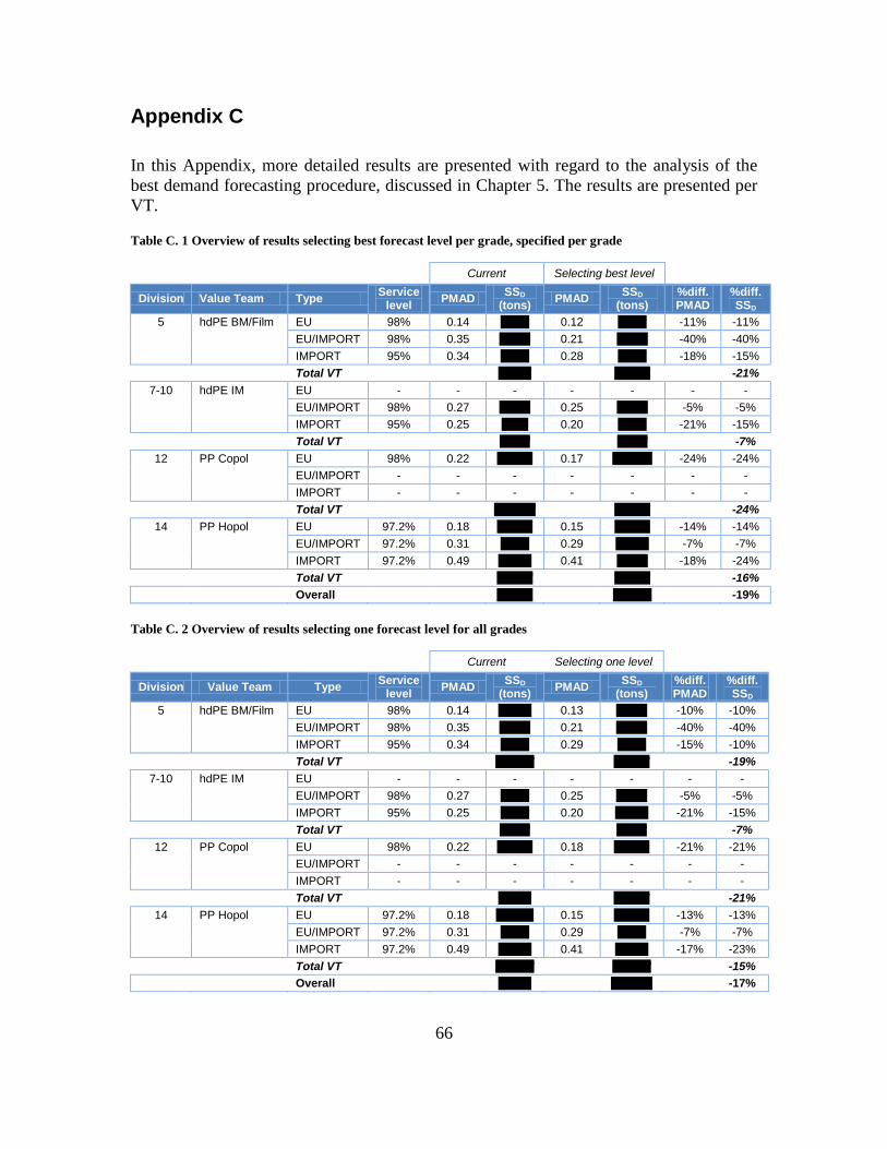
66
Appendix C
In this Appendix, more detailed results are presented with regard to the analysis of the
best demand forecasting procedure, discussed in Chapter 5. The results are presented per
VT.
Table C. 1 Overview of results selecting best forecast level per grade, specified per grade
Current Selecting best level
Division Value Team Type Service
level PMAD
SSD (tons)
PMAD SSD
(tons) %diff. PMAD
%diff. SSD
5 hdPE BM/Film EU 98% 0.14 ''''''''''''' 0.12 ''''''''''''' -11% -11%
EU/IMPORT 98% 0.35 '''''''''''''' 0.21 '''''''''''''' -40% -40%
IMPORT 95% 0.34 ''''''''''''' 0.28 ''''''''''''' -18% -15%
Total VT
''''''''''''
'''''''''''''
-21%
7-10 hdPE IM EU - - - - - - -
EU/IMPORT 98% 0.27 '''''''''''''' 0.25 '''''''''''''' -5% -5%
IMPORT 95% 0.25 '''''''''''' 0.20 ''''''''''''' -21% -15%
Total VT
'''''''''''
'''''''''''
-7%
12 PP Copol EU 98% 0.22 '''''''''''''''' 0.17 '''''''''''''''''' -24% -24%
EU/IMPORT - - - - - - -
IMPORT - - - - - - -
Total VT
'''''''''''''''
'''''''''''''
-24%
14 PP Hopol EU 97.2% 0.18 '''''''''''''''' 0.15 '''''''''''''''' -14% -14%
EU/IMPORT 97.2% 0.31 ''''''''''''' 0.29 ''''''''''''''' -7% -7%
IMPORT 97.2% 0.49 ''''''''''''''' 0.41 '''''''''''''' -18% -24%
Total VT
'''''''''''''
'''''''''''''
-16%
Overall
'''''''''''''
''''''''''''''
-19%
Table C. 2 Overview of results selecting one forecast level for all grades
Current Selecting one level
Division Value Team Type Service
level PMAD
SSD (tons)
PMAD SSD
(tons) %diff. PMAD
%diff. SSD
5 hdPE BM/Film EU 98% 0.14 ''''''''''''''' 0.13 '''''''''''''' -10% -10%
EU/IMPORT 98% 0.35 '''''''''''''' 0.21 '''''''''''''' -40% -40%
IMPORT 95% 0.34 ''''''''''''' 0.29 ''''''''''''' -15% -10%
Total VT
''''''''''''''
'''''''''''''
-19%
7-10 hdPE IM EU - - - - - - -
EU/IMPORT 98% 0.27 ''''''''''''' 0.25 '''''''''''''' -5% -5%
IMPORT 95% 0.25 ''''''''''''' 0.20 ''''''''''''''' -21% -15%
Total VT
'''''''''''
'''''''''''
-7%
12 PP Copol EU 98% 0.22 '''''''''''''''' 0.18 '''''''''''''''' -21% -21%
EU/IMPORT - - - - - - -
IMPORT - - - - - - -
Total VT
''''''''''''
'''''''''''''
-21%
14 PP Hopol EU 97.2% 0.18 ''''''''''''''''' 0.15 '''''''''''''''' -13% -13%
EU/IMPORT 97.2% 0.31 ''''''''''''' 0.29 ''''''''''''' -7% -7%
IMPORT 97.2% 0.49 ''''''''''''''' 0.41 ''''''''''''''' -17% -23%
Total VT
''''''''''''''
''''''''''''''
-15%
Overall
''''''''''''
'''''''''''''''
-17%
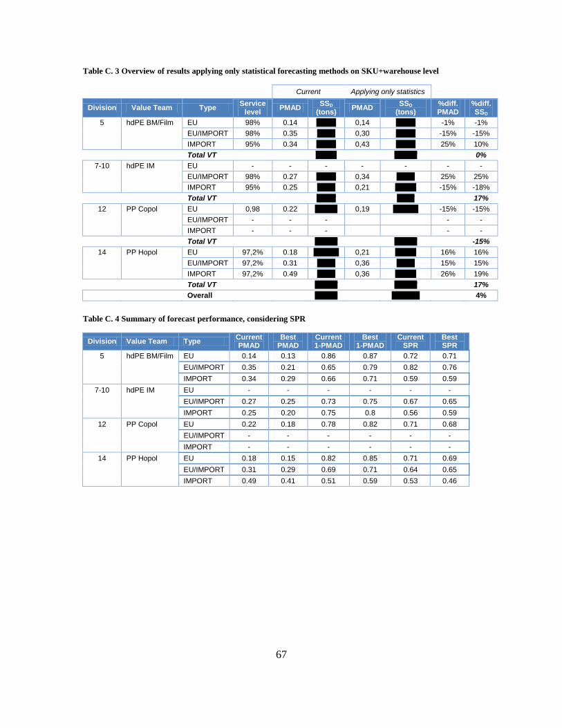
67
Table C. 3 Overview of results applying only statistical forecasting methods on SKU+warehouse level
Current Applying only statistics
Division Value Team Type Service
level PMAD
SSD (tons)
PMAD SSD
(tons) %diff. PMAD
%diff. SSD
5 hdPE BM/Film EU 98% 0.14 '''''''''''''' 0,14 '''''''''''''' -1% -1%
EU/IMPORT 98% 0.35 ''''''''''''' 0,30 '''''''''''''' -15% -15%
IMPORT 95% 0.34 '''''''''''''' 0,43 '''''''''''''' 25% 10%
Total VT
''''''''''''
'''''''''''''
0%
7-10 hdPE IM EU - - - - - - -
EU/IMPORT 98% 0.27 '''''''''''''' 0,34 ''''''''''''' 25% 25%
IMPORT 95% 0.25 ''''''''''''' 0,21 ''''''''''''''' -15% -18%
Total VT
'''''''''''
''''''''''
17%
12 PP Copol EU 0,98 0.22 '''''''''''''''' 0,19 '''''''''''''''''' -15% -15%
EU/IMPORT - - -
- -
IMPORT - - -
- -
Total VT
'''''''''''''
'''''''''''''
-15%
14 PP Hopol EU 97,2% 0.18 '''''''''''''''''' 0,21 ''''''''''''''' 16% 16%
EU/IMPORT 97,2% 0.31 ''''''''''''' 0,36 ''''''''''''' 15% 15%
IMPORT 97,2% 0.49 ''''''''''''' 0,36 ''''''''''''''' 26% 19%
Total VT
'''''''''''''
'''''''''''''
17%
Overall
''''''''''''' ''''''''''''''''
4%
Table C. 4 Summary of forecast performance, considering SPR
Division Value Team Type Current PMAD
Best PMAD
Current 1-PMAD
Best 1-PMAD
Current SPR
Best SPR
5 hdPE BM/Film EU 0.14 0.13 0.86 0.87 0.72 0.71
EU/IMPORT 0.35 0.21 0.65 0.79 0.82 0.76
IMPORT 0.34 0.29 0.66 0.71 0.59 0.59
7-10 hdPE IM EU - - - - - -
EU/IMPORT 0.27 0.25 0.73 0.75 0.67 0.65
IMPORT 0.25 0.20 0.75 0.8 0.56 0.59
12 PP Copol EU 0.22 0.18 0.78 0.82 0.71 0.68
EU/IMPORT - - - - - -
IMPORT - - - - - -
14 PP Hopol EU 0.18 0.15 0.82 0.85 0.71 0.69
EU/IMPORT 0.31 0.29 0.69 0.71 0.64 0.65
IMPORT 0.49 0.41 0.51 0.59 0.53 0.46

68
Forecast bias overview
Here a more detailed overview of the results of the forecast bias analysis are presented. Table C. 5 Bias analysis VT hdPE BM/Film
'''''''''''''''' '''''''''''' ''''''''''''' '''''''''' '''''''''''' ''''''''''''''''''' ''''''''' '''''''''''''''
''' '''''''''''''' ''''''''''''''''''' '''''''' '''''''''''''''' '''''''''''''''' ''''''''' '''''''''''
' '' '''''''' ''''''''''''''' ''''''''''''''' ''''''''''' '''''''''''
' '' ''''''' ''''''''''''''' ''''''''''''''' '''''''''''' ''''''''''
' '' '''''''' '''''''''''''''' ''''''''''''''' '''''''''' ''''''''''
' '' ''''''' '''''''''''''''' ''''''''''''''' ''''''''''' ''''''''''
' '' '''''''' ''''''''''''''' '''''''''''''''' '''''''''''' ''''''''''
' '' ''''''' ''''''''''''''' ''''''''''''''' '''''''''''' ''''''''''
' '' ''''''' ''''''''''''''' '''''''''''''''' '''''''''''' ''''''''''
' '' ''''''' ''''''''''''''''' '''''''''''''''' '''''''''' '''''''''
'' '' ''''''' '''''''''''''''''''' ''''''''''''''' ''''''''' '''''''''''
'' '' '''''''' ''''''''''''''''''''''''''''''''' '''''''''''''''' '''''''''''' ''''''''''
' '' '''''''' '''''''''''''''''''''''''''' ''''''''''''''' ''''''''' '''''''''''
'' '' '''''''' ''''''''''''''''''''''''' '''''''''''''' ''''''''' '''''''''
'' '' ''''''' ''''''''''''''''''''''''''''' ''''''''''''''' '''''''''' ''''''''''
' '' '''''''' '''''''''''''''''''''' ''''''''''''''' ''''''''''' '''''''''''
' '' ''''''''''''''''''''''''''' '''''''''''''''''''''' '''''''''''''' '''''''''''' ''''''''''''
' '' '''''''''''''''''''''' ''''''''''''''' '''''''''''''''' ''''''''''' ''''''''''''
' '' ''''''''''''''''''' ''''''''''''''' ''''''''''''''' ''''''''''''' '''''''''
' '' ''''''''''''''''''''''' ''''''''''''''''''''' '''''''''''''''' ''''''''''' '''''''''''
'' '' ''''''''''''''''''' '''''''''''''''' '''''''''''''' ''''''''' '''''''''
' '' '' '''''''''''''' ''''''''''''' ''''''''''
Table C. 6 Bias analysis VT hdPE IM
'''''''''''''''''' ''''''''''' '''''''''' ''''''''''' '''''''''''' ''''''''''''''''' '''''''''' ''''''''''''''''
'''''''''''' '''''''''''''' '''''' '''''''''''''''''''''''''''' ''''''''''''''''''''''''' '''''''''''''' ''''''''''''' ''''''''''
''''''''''''''''''''''''''''''' ''''''''''''''''''''' ''''''''''''''''' '''''''''''' '''''''''
''''''''''''''''''''''''''' ''''''''''''''''''''''' '''''''''''''''' ''''''''''''' '''''''''''
''''''''''''''''''' ''''''''''''''''''''' '''''''''''''' ''''''''''' ''''''''''
''''''''''''''''''' '''''''''''''''''''' '''''''''''''''' '''''''''''' ''''''''''
'''''''''''''''''''' '''''''''''''''''''' '''''''''''''''' '''''''''' ''''''''''
'' '' '' ''''''''''''''' ''''''''''''' '''''''''''
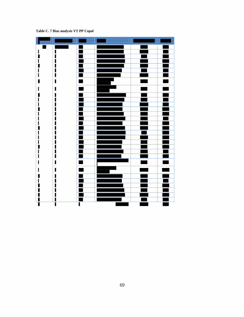
69
Table C. 7 Bias analysis VT PP Copol
''''''''''''''''''
''''''''''' ''''''''''' '''''''''' '''''''''''' '''''''''''''''''' ''''''''' ''''''''''''''
'''''' '''''''' ''''''''''''' ''''''' ''''''''' ''''''' '''''' ''''''''''''''' '''''''''''' ''''''''''
' '' ''''''' ''''''''' '''''''' '''''' '''''''''''''' '''''''''''''' '''''''''
'' '' ''''''' ''''''''' ''''''''''' '''''' '''''''''''''' '''''''''' ''''''''''
' '' '''''''' ''''''''' '''''''' '''''' '''''''''''''''' ''''''''''''' '''''''''''
'' '' ''''''' '''''' ''''''''' ''''' '''''''''''''''' ''''''''''''' ''''''''
' '' '''''''' ''''''''''''''' '''''''''''''''' '''''''''' '''''''''
' '' ''''''' ''''''''''''''' '''''''''''''' '''''''''''''' '''''''''
'' '' ''''''' '''''''''''''''''''''''''''' '''''''''''''''''''''''
'''''''''''' '''''''''
' '' '''''''' '''''''''''''''''''''''''''''''' '''''''''''''''''''''
''''''''''' ''''''''
'' '' ''''''' '''''''' '''''''''''' '''''' '''''''''''''''' '''''''''' ''''''''''
' '' '''''''' ''''''''' '''''''' '''''' ''''''''''''''' ''''''''''' '''''''''
' '' '''''''' '''''' ''''' '''''' ''''''''''''''' '''''''''''''' ''''''''
'' '' ''''''' '''''' '''' ''''''' ''''''''''''''' ''''''''''''' '''''''''
' '' ''''''' '''''''' ''''''''' '''''' '''''''''''''' '''''''''''' '''''''''''
' '' '''''''' '''''''' ''''''''''''' '''''' '''''''''''''' '''''''''''' '''''''''
' '' ''''''' '''''' ''''' '''''' ''''''''''''''' ''''''''''''' '''''''''''
'' '' '''''''' '''''' '''''''''''' '''''' ''''''''''''''' ''''''''''''' '''''''''''
' '' ''''''' ''''''''' ''''''''' ''''''' ''''''''''''''' ''''''''' '''''''''''
' '' ''''''' ''''' '''''''' ''''''' ''''''' '''''''''''''' ''''''''''''' '''''''''''
' '' '''''''' ''''' '''''''' '''''' '''''''''''''' ''''''''''' '''''''''''
'' '' '''''''' ''''' ''''''' '''''' '''''''''''''' ''''''''''' '''''''''''
' '' ''''''' ''''''' '''''''' '''''' '''''''''''''' '''''''''''' '''''''''
' '' ''''''' ''''''''''''''' ''''''''''''''' ''''''''''''' ''''''''''
' '' ''''''' '''''''''''''''''''''''''''''''''''''''''''''''''''''
''''''''''' ''''''''''
' '' '''''''' '''''''''''''''''''''''''''''''' '''''''''''''''''''''
'''''''''''''' ''''''''''''
'' '' ''''''' ''''''''''' '''''' ''''''''''''''' '''''''''''' '''''''''''
' '' '''''''' '''''''''' ''''' '''''''''''''''' '''''''''''' '''''''''
'' '' ''''''' ''''''''''' ''''' ''''' ''''''''''''''' '''''''''''' '''''''''
'' '' ''''''' ''''''''''''' '''''' '''''''''''''''' ''''''''''' ''''''''''
'' '' '''''''' ''''''''''' ''''''' '''''' ''''''''''''''' '''''''''''''' '''''''''''
'' '' ''''''' '''''''''''''''' '''''''''''''''' '''''''''' ''''''''''
'' '' '' ''''''''''''''''' '''''''''''''' ''''''''''

70
Table C. 8 Bias analysis VT PP Hopol
'''''''''''''''' ''''''''''' '''''''''''' ''''''''''' '''''''''''''' ''''''''''''''''''' ''''''''' ''''''''''''''
'''''' ''''''' ''''''''''''''' ''''''''''''''''''''''''''' '''''''''''' ''''''''''''''' ''''''''''' ''''''''''''
''''''''''''''''''''''''''''''' ''''''''''''' '''''''''''''''' ''''''''''''' ''''''''''
'''''''' ''''''''''''' '''''''''''''''' '''''''''''' '''''''''''
''''''' '''''''''''' '''''''''''''' ''''''''' '''''''''
'''''''' ''''''''''''' '''''''''''''''' '''''''''''' ''''''''
''''''' '''''''''''' ''''''''''''''' ''''''''''''' ''''''''''''
'''''''' '''''''''''' ''''''''''''''' '''''''''''' ''''''''''''
'''''''' '''''''''''' ''''''''''''''' '''''''''''' ''''''''
''''''' ''''''''''' ''''''''''''''' '''''''''''' ''''''''''''
'''''''' ''''''''''''' '''''''''''''''' '''''''''''' '''''''''
'''''''' ''''''''''''' '''''''''''''''' '''''''''''' '''''''''
'''''''' '''''''''''''' '''''''''''''' '''''''''' '''''''''''
'''''''' '''''''''''''' ''''''''''''''' '''''''''' ''''''''''
''''''' '''''''''''''' ''''''''''''''' '''''''''''' '''''''''''
''''''' '''''''''''''' ''''''''''''''' ''''''''' '''''''''''
''''''' '''''''''''' '''''''''''''''' ''''''''''' '''''''''
''''''' ''''''''''' '''''''''''''''' ''''''''''' '''''''''
'''''''' '''''''''''''' '''''''''''''' '''''''''' ''''''''''
'''''''' '''''''''''''' '''''''''''''' '''''''''' ''''''''''
''''''' '''''''''''' '''''''''''''''' '''''''''''' '''''''''
''''''' '''''''''''' '''''''''''''' '''''''''' '''''''''''
'''''''' '''''''''''''''' '''''''''''''''' ''''''''''' ''''''''''
''''''' '''''''''''' ''''''''''''''' ''''''''''''' ''''''''
''''''' ''''''''''''' ''''''''''''''' ''''''''''' '''''''''''
''''''' '''''''''' ''''' '''''''''''''''' '''''''''''' ''''''''''''
''''''' ''''''''''''''''''' ''''''''''''''' ''''''''''' '''''''''''
''''''' '''''''''''''''''''''' '''''''''''''''' ''''''''''' '''''''''''
''''''' '''''''''''''''''''' ''''''''''''''' ''''''''' ''''''''''
'''''''' '''''''' ''''' ''''''''' ''''' ''''''''''''''' '''''''''''' ''''''''''
''''''' '''''''''' '''' '''''' '''''''''''''' ''''''''''' ''''''''''''
'''''''''''''''''''''' ''''''''''''' ''''''''''''''' '''''''''''' ''''''''''
''''''''''''''''''' '''''''''''''' '''''''''''''''' ''''''''' '''''''''''
'''''''''''''''''''' ''''''''''''' ''''''''''''''' ''''''''''' ''''''''
'''''''''''''''''''' '''''''''''''' ''''''''''''''' ''''''''''''' '''''''''''
''''''''''''''''''''' '''''''''''' ''''''''''''''' ''''''''''' '''''''''''
'''''''''''''''''''' '''''''''''''' '''''''''''''' '''''''''''' ''''''''''
''''''''''''''''''''' '''''''''''''' '''''''''''''' ''''''''''' ''''''''''
'''''''''''''' '''''''''''''' '''''''''''
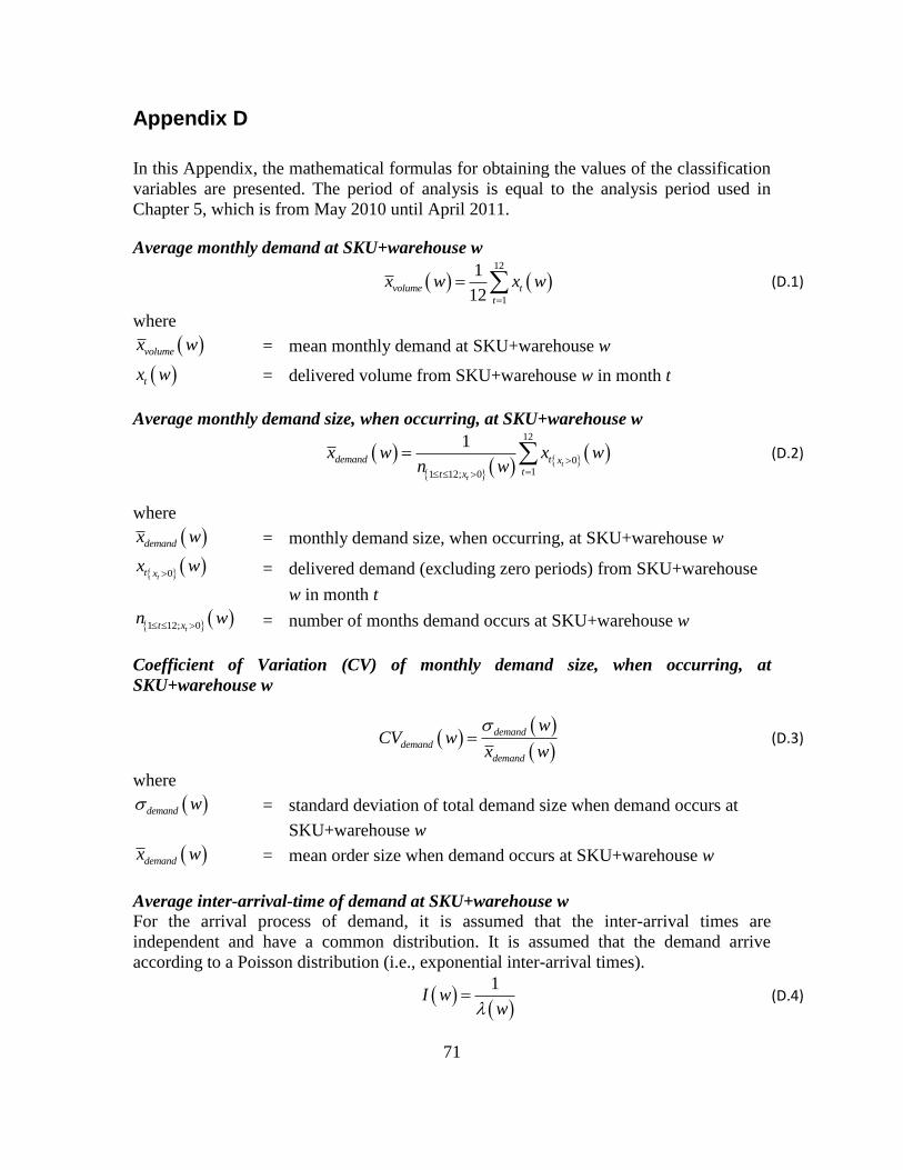
71
Appendix D
In this Appendix, the mathematical formulas for obtaining the values of the classification
variables are presented. The period of analysis is equal to the analysis period used in
Chapter 5, which is from May 2010 until April 2011.
Average monthly demand at SKU+warehouse w
12
1
1
12volume t
t
x w x w
(D.1)
where
volumex w = mean monthly demand at SKU+warehouse w
tx w = delivered volume from SKU+warehouse w in month t
Average monthly demand size, when occurring, at SKU+warehouse w
12
011 12; 0
1t
t
demand t xtt x
x w x wn w
(D.2)
where
demandx w
= monthly demand size, when occurring, at SKU+warehouse w
0tt x
x w = delivered demand (excluding zero periods) from SKU+warehouse
w in month t
1 12; 0tt xn w
= number of months demand occurs at SKU+warehouse w
Coefficient of Variation (CV) of monthly demand size, when occurring, at
SKU+warehouse w
demand
demand
demand
wCV w
x w
(D.3)
where
demand w = standard deviation of total demand size when demand occurs at
SKU+warehouse w
demandx w = mean order size when demand occurs at SKU+warehouse w
Average inter-arrival-time of demand at SKU+warehouse w
For the arrival process of demand, it is assumed that the inter-arrival times are
independent and have a common distribution. It is assumed that the demand arrive
according to a Poisson distribution (i.e., exponential inter-arrival times).
1
I ww
(D.4)
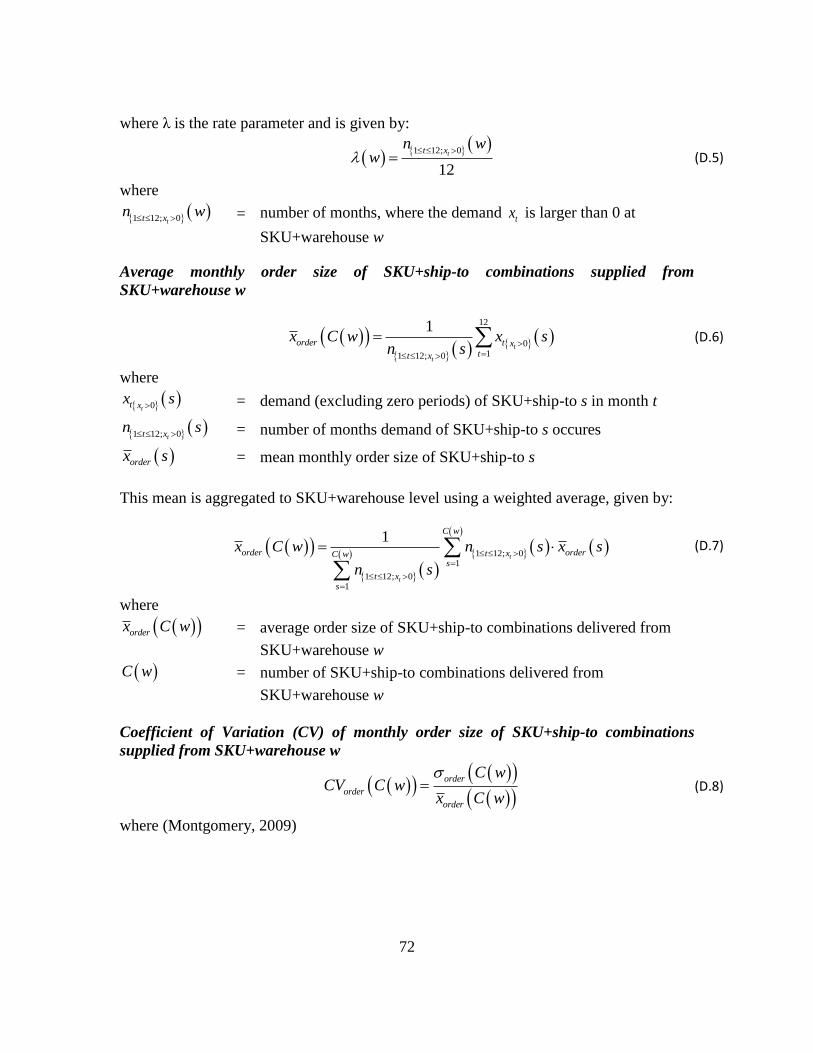
72
where λ is the rate parameter and is given by:
1 12; 0
12
tt xn w
w
(D.5)
where
1 12; 0tt xn w
= number of months, where the demand tx is larger than 0 at
SKU+warehouse w
Average monthly order size of SKU+ship-to combinations supplied from
SKU+warehouse w
12
011 12; 0
1t
t
order t xtt x
x C w x sn s
(D.6)
where
0tt x
x s
= demand (excluding zero periods) of SKU+ship-to s in month t
1 12; 0tt xn s
= number of months demand of SKU+ship-to s occures
orderx s = mean monthly order size of SKU+ship-to s
This mean is aggregated to SKU+warehouse level using a weighted average, given by:
1 12; 01
1 12; 01
1t
t
C w
order ordert xC ws
t xs
x C w n s x s
n s
(D.7)
where
orderx C w = average order size of SKU+ship-to combinations delivered from
SKU+warehouse w
C w = number of SKU+ship-to combinations delivered from
SKU+warehouse w
Coefficient of Variation (CV) of monthly order size of SKU+ship-to combinations
supplied from SKU+warehouse w
order
order
order
C wCV C w
x C w
(D.8)
where (Montgomery, 2009)
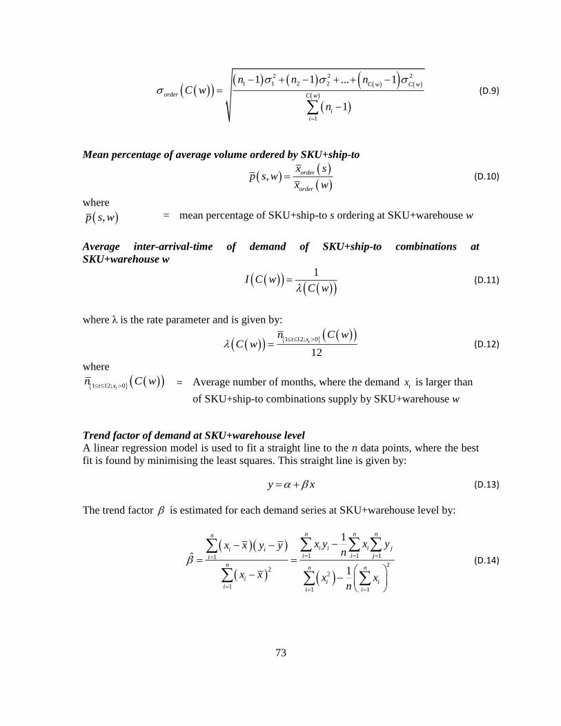
73
2 2 2
1 1 2 2
1
1 1 ... 1
1
C w C w
order C w
i
i
n n nC w
n
(D.9)
Mean percentage of average volume ordered by SKU+ship-to
,
order
order
x sp s w
x w (D.10)
where
,p s w = mean percentage of SKU+ship-to s ordering at SKU+warehouse w
Average inter-arrival-time of demand of SKU+ship-to combinations at
SKU+warehouse w
1I C w
C w (D.11)
where λ is the rate parameter and is given by:
1 12; 0
12
tt xn C w
C w
(D.12)
where
1 12; 0tt xn C w
= Average number of months, where the demand tx is larger than
of SKU+ship-to combinations supply by SKU+warehouse w
Trend factor of demand at SKU+warehouse level
A linear regression model is used to fit a straight line to the n data points, where the best
fit is found by minimising the least squares. This straight line is given by:
y x (D.13)
The trend factor is estimated for each demand series at SKU+warehouse level by:
1 1 11
22
2
11 1
1
ˆ
1
n n nn
i i i ji ii i ji
nn n
ii i
ii i
x y x yx x y yn
x x x xn
(D.14)
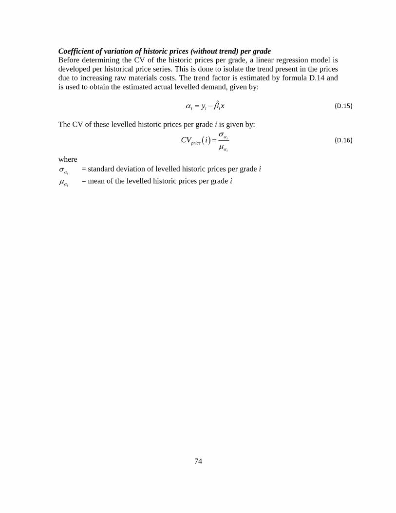
74
Coefficient of variation of historic prices (without trend) per grade
Before determining the CV of the historic prices per grade, a linear regression model is
developed per historical price series. This is done to isolate the trend present in the prices
due to increasing raw materials costs. The trend factor is estimated by formula D.14 and
is used to obtain the estimated actual levelled demand, given by:
ˆi i iy x (D.15)
The CV of these levelled historic prices per grade i is given by:
i
i
priceCV i
(D.16)
where
i = standard deviation of levelled historic prices per grade i
i = mean of the levelled historic prices per grade i
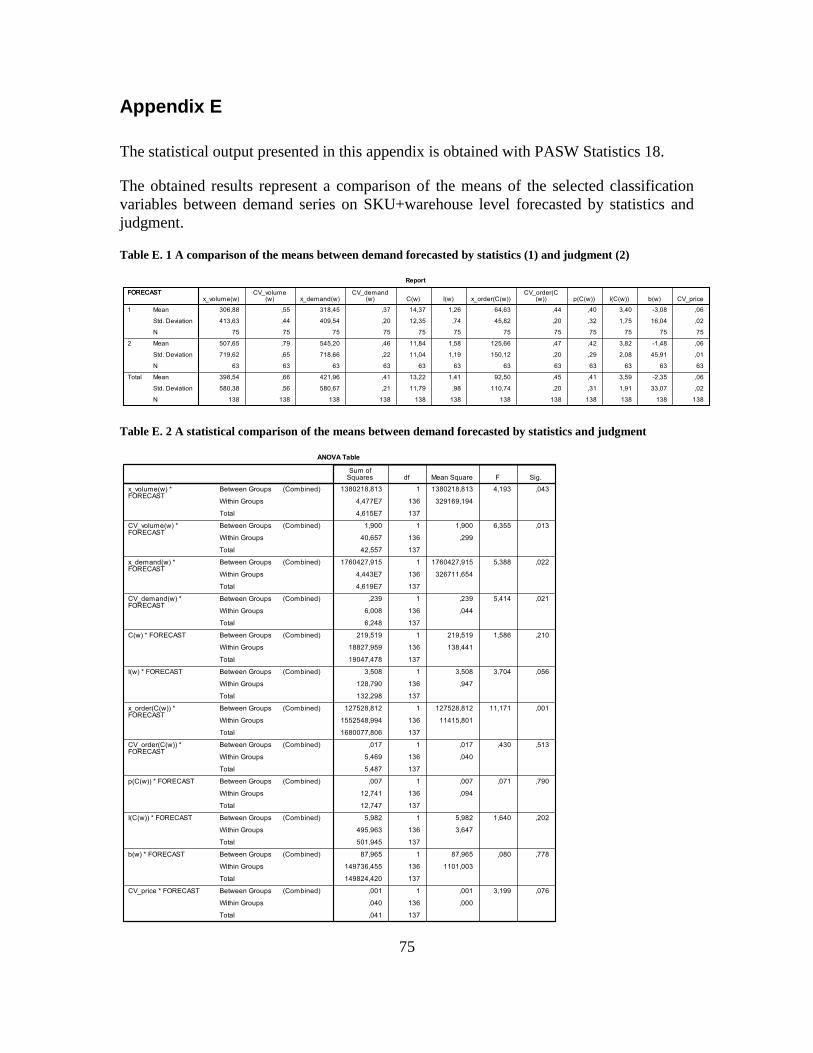
75
Appendix E
The statistical output presented in this appendix is obtained with PASW Statistics 18.
The obtained results represent a comparison of the means of the selected classification
variables between demand series on SKU+warehouse level forecasted by statistics and
judgment.
Table E. 1 A comparison of the means between demand forecasted by statistics (1) and judgment (2)
Table E. 2 A statistical comparison of the means between demand forecasted by statistics and judgment
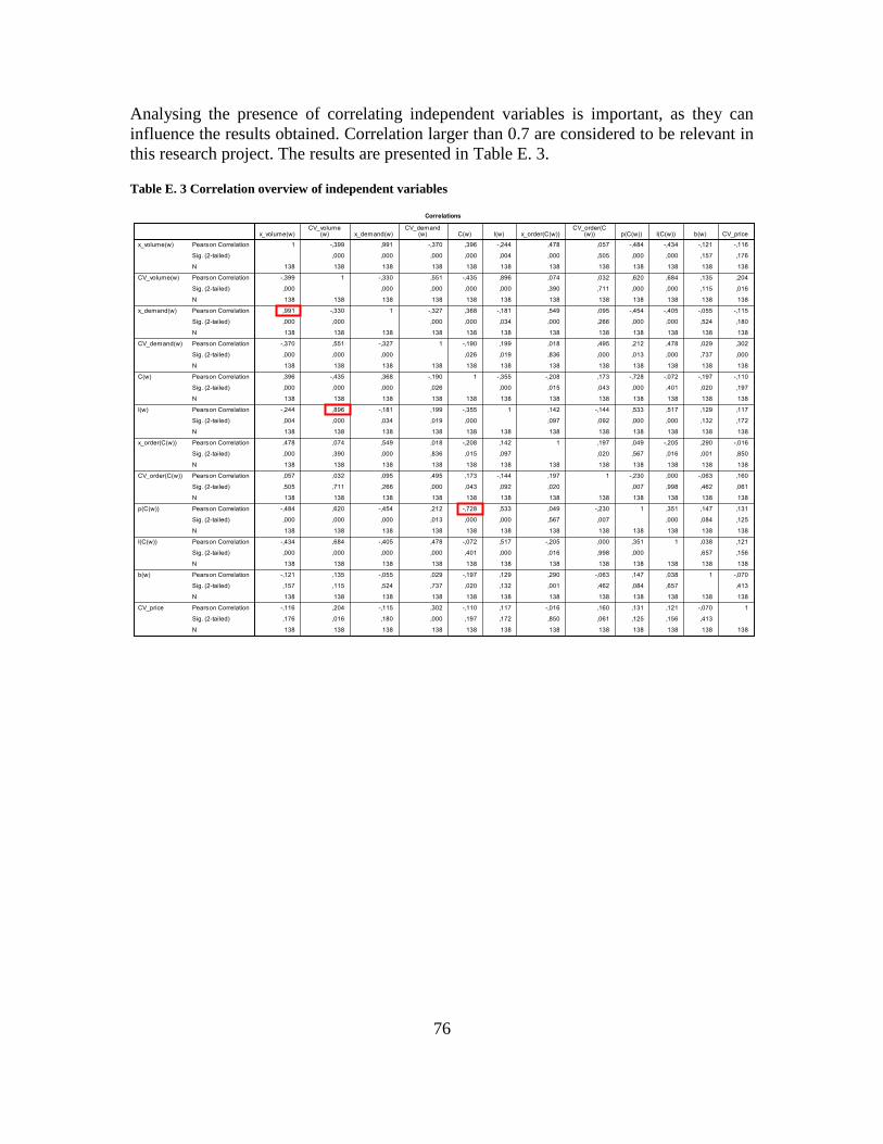
76
Analysing the presence of correlating independent variables is important, as they can
influence the results obtained. Correlation larger than 0.7 are considered to be relevant in
this research project. The results are presented in Table E. 3.
Table E. 3 Correlation overview of independent variables
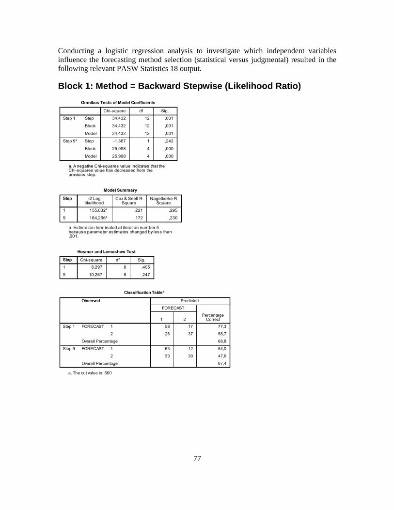
77
Conducting a logistic regression analysis to investigate which independent variables
influence the forecasting method selection (statistical versus judgmental) resulted in the
following relevant PASW Statistics 18 output.
Block 1: Method = Backward Stepwise (Likelihood Ratio)
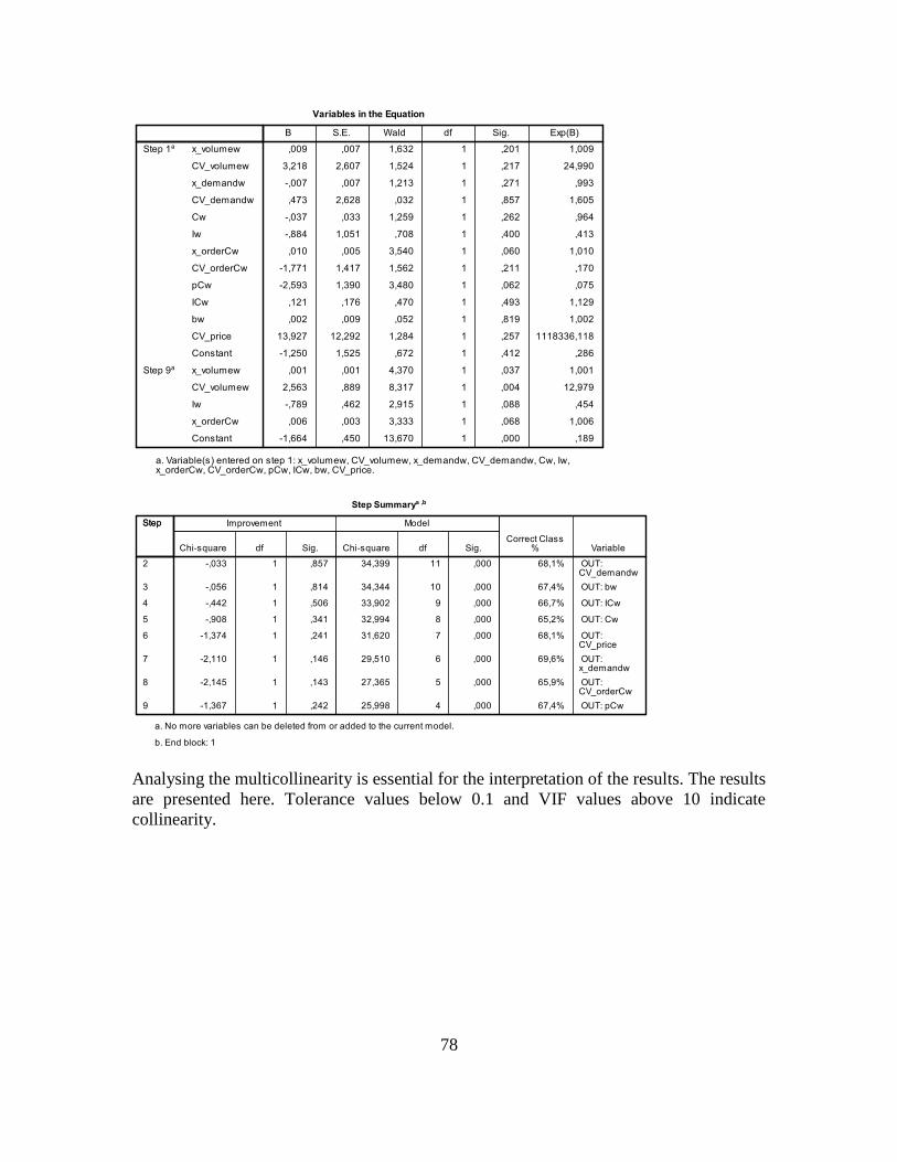
78
Analysing the multicollinearity is essential for the interpretation of the results. The results
are presented here. Tolerance values below 0.1 and VIF values above 10 indicate
collinearity.
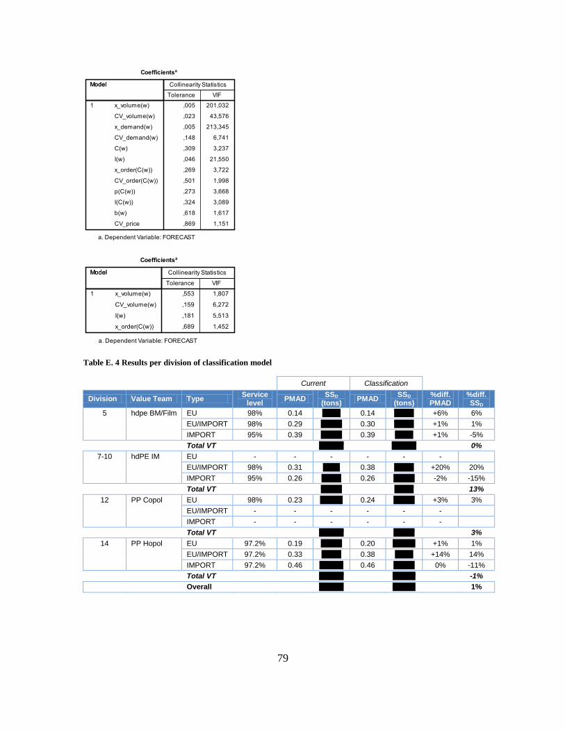
79
Table E. 4 Results per division of classification model
Current Classification
Division Value Team Type Service
level PMAD
SSD
(tons) PMAD
SSD
(tons) %diff. PMAD
%diff. SSD
5 hdpe BM/Film EU 98% 0.14 ''''''''''''' 0.14 '''''''''''''' +6% 6%
EU/IMPORT 98% 0.29 ''''''''''''''' 0.30 '''''''''''''' +1% 1%
IMPORT 95% 0.39 ''''''''''''''' 0.39 ''''''''''''' +1% -5%
Total VT
''''''''''''''
''''''''''''''
0%
7-10 hdPE IM EU - - - - - -
EU/IMPORT 98% 0.31 '''''''''''' 0.38 '''''''''''''' +20% 20%
IMPORT 95% 0.26 '''''''''''''' 0.26 ''''''''''''''' -2% -15%
Total VT
''''''''''''
'''''''''''
13%
12 PP Copol EU 98% 0.23 '''''''''''''''' 0.24 ''''''''''''''' +3% 3%
EU/IMPORT - - - - - -
IMPORT - - - - - -
Total VT
''''''''''''''
''''''''''''
3%
14 PP Hopol EU 97.2% 0.19 ''''''''''''''' 0.20 '''''''''''''''' +1% 1%
EU/IMPORT 97.2% 0.33 '''''''''''''' 0.38 ''''''''''''' +14% 14%
IMPORT 97.2% 0.46 ''''''''''''''''' 0.46 ''''''''''''''' 0% -11%
Total VT
''''''''''''''
'''''''''''''
-1%
Overall
''''''''''''''
'''''''''''''
1%
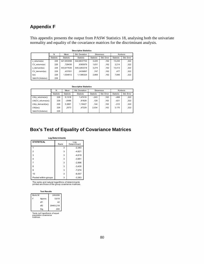
80
Appendix F
This appendix presents the output from PASW Statistics 18, analysing both the univariate
normality and equality of the covariance matrices for the discriminant analysis.
Box's Test of Equality of Covariance Matrices