econometric forecasting · econometrics. no doubt, ... second, econometric forecasting lost...
TRANSCRIPT
Principles of Forecasting: A Handbook for Researchers and Practitioners, J. Scott Armstrong (ed.): Norwell, MA: Kluwer Academic Publishers, 2001
Econometric Forecasting
P. Geoffrey Allen Department of Resource Economics
University of Massachusetts, Amherst MA 01003, USA and
Robert Fildes Department of Management Science
University of Lancaster, Lancaster LA 1 4YX, UK
ABSTRACT
Several principles are useful for econometric forecasters: keep the model simple, use all the data you
can get, and use theory (not the data) as a guide to selecting causal variables. But theory gives little
guidance on dynamics, that is, on which lagged values of the selected variables to use. Early
econometric models failed in comparison with extrapolative methods because they paid too little
attention to dynamic structure. In a fairly simple way, the vector autoregression (VAR) approach that
first appeared in the 1980s resolved the problem by shifting emphasis towards dynamics and away
from collecting many causal variables. The VAR approach also resolves the question of how to make
long-term forecasts where the causal variables themselves must be forecast. When the analyst does not
need to forecast causal variables or can use other sources, he or she can use a single equation with the
same dynamic structure. Ordinary least squares is a perfectly adequate estimation method. Evidence
supports estimating the initial equation in levels, whether the variables are stationary or not. We
recommend a general-to-specific model-building strategy: start with a large number of lags in the
initial estimation, although simplifying by reducing the number of lags pays off. Evidence on the value
of further simplification is mixed. If cointegration among variables, then error-correction models
(ECMs) will do worse than equations in levels. But ECMs are only sometimes an improvement even
when variables are cointegrated. Evidence is even less clear on whether or not to difference variables
that are nonstationary on the basis of unit root tests. While some authors recommend applying a battery
of misspecification tests, few econometricians use (or at least report using) more than the familiar
Durbin-Watson test. Consequently, there is practically no evidence on whether model selection based
on these tests will improve forecast performance. Limited evidence on the superiority of varying
parameter models hints that tests for parameter constancy are likely to be the most important. Finally,
econometric models do appear to be gaining over extrapolative or judgmental methods, even for short-
term forecasts, though much more slowly than their proponents had hoped.
Keywords: econometric forecasting, vector autoregression, error correction model, specification testing, forecast
comparisons

ECONOMETRIC FORECASTING 2
INTRODUCTION Historical background Econo-magic and Economic tricks are two of the pejorative terms its detractors use to describe the art and science of econometrics. No doubt, these terms are well deserved in many instances. Some of the problems stem from econometrics= connection with statistics, which had its origin in the analysis of experimental data. In the typical experiment, the analyst can hold the levels of variables not of interest constant, alter the levels of treatment variables, and measure both the treatment variables and the outcome with high accuracy. With some confidence, the statistician can assert that changes in the treatment variable cause changes in the outcome and can quantify the relationship.
Analysts began to apply the statistical tools appropriate to this experimental setting to economic and business data that were clearly not the outcome of any experiment. The question of cause and effect became murky. Statisticians relied on economic theory to guide them; they had few other choices. So was born econometrics: the use of statistical analysis, combined with economic theory, to analyze economic data.
One of the pioneers of econometric forecasting was Charles Sarle (Sarle, 1925). His essay describing a single equation model to forecast the price of hogs won the Babson prize in 1925 and was published in a special supplement to the American Economic Review. The Babson prize was awarded for the best essay submitted by a student, as judged by a committee of eminent economists. At $650, the prize could have bought young Charles his first car. Sarle was several decades ahead of his time. He used lagged explanatory variables, so their values were known at the time of forecast; he performed both within-sample and out-of-sample forecasts. Although his work was published in the leading economic journal, it was then largely ignored. Such is the fate of many a pioneer. Why this occurred is the subject of a fascinating reappraisal of Sarle=s work by Gordon and Kerr (1997). With the advantage of modern techniques and computing power, Gordon and Kerr determined that Sarle=s model was reasonably well specified. They surmise that it remained unknown for two reasons. First, Ezekiel, who did become well-known, wrote a subsequent article in which he criticized Sarle=s choice of variables. Second, econometric forecasting lost popularity shortly after publication of Sarle=s article. It reappeared in the mid 1950s, by which time articles published in the 1920s had been largely forgotten.
Econometricians are a diverse and large group of quantitative analysts. For the last 60 years or so, the group has focused on one key problem: that nonexperimental data, violates many of the statisticians= standard assumptions. Although Leamer (1983), in his classic article ALet=s take the con out of econometrics,@ asserted that the difference between experimental and nonexperimental data was only one of degree, most econometricians would argue that the degree of difference is large enough to matter. Unfortunately for forecasters, research by econometricians= has not focused on what works best with real-world data, but on which particular method would be optimal if a standard assumption is violated in some well-defined way. As a result, the findings in Aclassical econometrics@ are of limited value. More promising is the work of the new wave of time series econometricians who draw from the philosophies of time series forecasters. These econometricians use economic theory for what it can do, which is give guidance on long-term cause-and-effect relationships. Short-term dynamics, mainly expressed by lags on variables and by differencing, are selected to be congruent with the data. To that extent, they allow the data to determine the structure of the model.
The principal tool of the econometrician is regression analysis, using several causal variables. Other methods of causal modeling exist, but they are not discussed in this chapter. Compared with univariate modeling, multivariate analysis opens up many more choices for the investigator: the set of variables to include in the analysis; the structure, that is, the number of equations relating the set of variables to each other and the causal variables to use in each equation, if more than one equation is included; and the functional form of the equation: whether it is linear or nonlinear in parameters.
The fundamental principle
With the range of choices just described, coming up with a universally acceptable strategy is difficult, though we will suggest one later. Some econometric forecasters may disagree with us over the details, but all should agree with the overall principle:
! Aim for a relatively simple model specification. This principle applies to most kinds of quantitative forecasting. Simplicity in analysis is an old concept, in
econometrics going back at least to Haavelmo=s (1944) classic treatise (pp. 22-23): AOur hope in economic theory and research is that it may be possible to establish constant and relatively simple relations between dependent variables . . . and a relatively small number of independent variables (italics in original)@. (See chapter 1 for more discussion.) What Haavelmo means by Arelatively simple@ is a good question. He does not reach a conclusion and, a few lines lower down, seems to argue for out-of-sample testing as the final judge: AWhether or not such simple relations can be established must be decided by actual trials.@
An econometric model can be too simple. That is, a more complex model (e.g., containing more independent variables and having a nonlinear structure) may give both better within sample fit than a simpler model and, critically,

PRINCIPLES OF FORECASTING
3
better out-of-sample forecast accuracy. Zellner (1992) recognized this danger with his KISS principle (Keep It Sophisticatedly Simple). But an all-too-common occurrence is to discover that an econometric model gives worse forecasts than the naive no change method or than exponential smoothing. Such failure might arise because the analyst needs to forecast a causal variable and can do so only with difficulty. For pure forecasting, a casual variable should be included only if its value is known or if it can be forecast reasonably accurately. (We return to the question of how to quantify Areasonably@ later in the chapter.) If the purpose of the model is policy analysis (that is, to answer some form of what if question) then the question is: does inclusion of the causal variable, with the value that actually occurred, give a more accurate prediction of the dependent variable, when tested on data not used to estimate parameters, than exclusion of the variable? Those who think the answer to the question is Aalways@ may find the next paragraph disturbing.
An overriding axiom for econometricians is that any model is a misspecification of the process that generated the data; what is wanted is a model and estimation procedure that is robust to misspecification. Gilbert (1995) made a pointed argument for parsimony (p. 230): AOne surprising result is that, for prediction purposes, knowledge of the true structure of the model generating the data is not particularly useful unless parameter values are also known. This is because the error in estimating parameters of the true model causes more prediction error than is obtained from a more parsimonious approximate model.@ Gilbert arrived at his finding through Monte Carlo simulation, a method often used to test how econometric theories perform in practice. He created a series of true values of a variable based on a known time series model. Then by adding a randomly generated error term to each true value he created an artificial sample of data and replicated the sample generation many times. He was then able to get many estimates both of the parameters of the true model and of the parameters of simpler models.
We have found no other studies that directly confirm Gilbert=s arguments, so we do not know how important are the degree of approximation of the simpler model to the true model and the relative magnitude of sources of randomness in data generation. But as further indirect empirical evidence that parsimony leads to better forecasts, we show later the lack of success of classical econometric models when compared with simpler methods.
A strategy for econometric forecasters
We propose a strategy based on the time-series econometrics approach. Each numbered step is discussed in detail in each of the major sections that follows the introduction. (1) Define the objectives of the modeling effort. Econometrics, like physics, lacks a universal model. For example, an equation that seems to explain how changes in a set of variables can cause a company=s annual sales to decrease may help managers understand the forces in the economy that influence their business. But unless the causal variables can be controlled, have long leads, or are easy to forecast, they will be useless in a model intended for forecasting. Similarly, if the objective is to answer a policy question, for example how increased advertising will increase sales, then advertising must be included as a causal variable. (2) Determine the set of variables to use based on economic theory and previous work. The initial list of variables can be lengthy, but one essential step is to whittle it down to about a six variables before estimation. Judgment is likely to be better than theory in deciding which are the most important variables. (3) Collect the data, generally as long a time series as possible. Use all the data unless this makes the model intractable. Events such as wars, changes in regulations, changes in company organization, or unusual weather may call for putting different weights on observations in different time periods, to the extreme of discarding from further analysis some part of the data, usually the oldest part. Such action should be the result of a conscious decision not of a less-than-diligent collection effort. At this stage, the variables must be specified precisely. Where there appear to be different definitions of a variable, the analyst must select one of the available definitions. If, as happens frequently, a desired data series does not exist, or perhaps exists as annual data when monthly data are required, then some less-perfect proxy variable must be collected instead. (4) Form an initial specification of the model. Using the variables decided on in step two, start with an autoregressive distributed-lag equation or its equivalent for a system of equations, a vector autoregression (VAR) model, with a fairly high lag order. At this stage, we do not believe that enough is known about the practical issues of working with a vector autoregressive moving average model (VARMA) to justify using one as a starting point. For one-step ahead forecasts, the single equation will be adequate, while for longer-term forecasts, a system of equations will almost always be needed. (The exception is when the value of every explanatory variable is either perfectly predictable - like the variable Atime@ - or is under the control of the agency that employs the forecaster.) In each equation, the dependent variable is a function of lagged values of itself and of all other variables. Such a specification is certainly not parsimonious and has been called Aprofligate in parameters.@ For example, a model with six variables and lags up to seventh order will require 42 parameters (plus a constant) in each equation, or a total of 252 parameters. It will also require estimation of 21 variances and covariances if hypothesis tests or variance decompositions are to be performed. While such models are better
ECONOMETRIC FORECASTING 4
forecasters than one might expect, comparative studies have shown a payoff from reducing the number of parameters. A VAR model has the following appeals:
(a) Each variable is in turn the dependent variable in an equation, and its lagged values are explanatory variables in each equation. (This is referred to as the VAR in standard form.) The arbitrary distinction between endogenous variables (those for which causal relations will be specified in the model) and exogenous variables (those taken as given) is avoided. Every variable is endogenous. (b) A general to specific modeling strategy is followed. Reduction in the number of parameters (that is, imposing zero or other restrictions on some of them) will improve forecast accuracy provided the reduced model still describes the data adequately. Misspecification tests (see step 6 below) assure the analyst that the parameter reductions are acceptable. (c) The problem of forecasting the causal variables is solved internally. Because each variable is in turn a dependent variable, predictions of all the variables of interest are automatically available. If one can forecast a causal variable by other means, such as by expert judgement, one does not need to be specify it as a dependent variable in an equation, which simplifies the model. (d) For any variable, one possible specification is a univariate model. This is a possible outcome of the general-to-specific strategy. While no moving average terms appear in such a model, by including enough lagged dependent variables, one can obtain a reasonable approximation of an autoregressive integrated moving-average (ARIMA) model. One objection to the VAR approach is that it is atheoretical. Perhaps more accurately, it uses theory only to get
the set of relevant variables. It does not use theory to define the cause-and-effect relation in each equation. The VAR in standard form is a system of reduced-form equations; each dependent variable is a function of the lagged values of all the variables. (5) Estimate the model. There seems to be no advantage from employing anything other than ordinary least squares regression. When the same set of regressors appears in each equation, as in an unrestricted VAR, ordinary least squares and generalized least squares are equivalent. When the equations have different sets of regressors, as in a restricted VAR, the seemingly unrelated regressions (SUR) form of generalized least squares or maximum-likelihood methods can be justified in theory but so far have not shown any advantage in practice. (6) Assess model adequacy by conducting misspecification tests. This is the heart of the time series econometrics approach that differentiates it from the classical econometrics approach. While these tests are helpful in pointing out problems with the model, their usefulness as a means of improving forecast accuracy is still an open question. (7) Simplify the model as much as possible by employing specification tests. Use specification tests to reduce the number of lags on the explanatory variables. Consider parameter restrictions that lead to error-correction models. The usual approach is to first test individual variables for the presence of unit roots, then to estimate the cointegrating equation or equations of the set of variables that possess unit roots. A cointegrating equation is essentially the regression of one of the variables on some or all of the rest of them, with only current or contemporaneous variables in the equation. Consider the more stringent restriction of imposing unit roots (by taking first differences of variables). Evidence is somewhat mixed, but if the simpler models derived from initial models by specification testing also pass misspecification tests, they do appear to provide better forecasts than more complex models. (8) Compare the out-of-sample performance of the final model or models against the performance of a benchmark model. Out-of-sample means data not used to estimate or test the model, usually the last several observations of the variable of interest. The model=s relative accuracy in forecasting the actual values of the variable is the usual criterion; its ability to predict turning points is less commonly used. The benchmark model is typically a univariate model; the naive no-change model is often a sufficiently challenging choice. If your carefully developed and tested econometric model cannot forecast better than such a simple alternative, all your effort has been in vain. DEFINE THE OBJECTIVES
! If explanation, including strategy analysis or policy analysis, is the purpose, then make conditional forecasts based on different values of control variables.
If the purpose of the study is to analyze a policy, such as a change in the excise tax rate on tobacco or a change in a firm=s advertising budget, then model structure is important. Ability to forecast causal variables is not. The econometrician may not know the values of the control variables, but the firm=s or government=s decision makers will. Their interest is in the response, for example, in sales or unemployment, to changes in factors they can control, for example, advertising or interest rates. To find out how much credence to give the model, make conditional forecasts outside the sample of data used in estimation, using actual values of explanatory variables. In other words, follow the same steps as you would when the model is purely for forecasting, with one difference: conduct conditional rather than unconditional forecast

PRINCIPLES OF FORECASTING
5
comparisons. It maybe bad news if sales show little response to advertising, or unemployment to interest rate reductions, but it is worth knowing.
Problems in making conditional policy forecasts lie at the heart of the famous ALucas critique@ (Lucas 1976). They arise because almost all economic relationships are behavioral rather than technical. That is, a rise in interest rates causes rational employers to decide to reduce the number of workers, which increases unemployment. Does a change in government policy, say, designed to stabilize interest rates alter the way in which decision makers respond to changes in rates? If not, there is no problem (the interest rate variable is Asuperexogenous@). If it does, there is some feedback from unemployment to interest rate and the new relationship between them cannot be estimated from past observations. Put another way, the parameter in the equation varies but in a way that is unknown to the econometrician.
! If pure forecasting is the purpose, you must be able to forecast explanatory variables sufficiently well to include them in a forecasting model.
If fundamental plant science says that the amount of moisture available in spring affects plant growth, an econometrician may be able to explain corn yield quite well on the basis of spring rainfall. But in the absence of good long-range weather forecasts, nothing will be gained from including a rainfall variable in a forecasting equation. Theory may suggest or require a particular causal variable in an equation, so that its omission is an error. But the error of omission may be less costly than the error in estimating the additional parameter. The simpler, yet incorrect model, may yield more accurate forecasts.
Ashley (1983) showed that ex post forecasts from a simple bivariate model with a contemporaneous causal variable and lagged dependent variables of low order were more accurate than forecasts from a benchmark univariate autoregressive model, provided actual historical data were used. But use of forecasts (of gross national product in one model, personal disposable income in another) from a Box-Jenkins method or from commercial macroeconomic forecasters, in place of actual historical data, led to ex post forecasts that were less accurate than the benchmark. Ashley established a simple theorem for the case of stationary variables: if the mean squared error (MSE) of the forecast of the causal variable exceeds its variance, then including the forecasted causal variable will produce worse forecasts than omitting it. Using the historical mean of the causal variable would produce better forecasts.
The proof of Ashley=s theorem assumes that the parameter on the causal variable is known. Since using an estimated coefficient increases error, the MSE of the forecast of the causal variable may have to be much less than its variance before inclusion of the variable improves forecasts. In a later paper, Ashley (1988) shows that forecasts of key macroeconomic variables from several commercial forecasters have MSEs that exceed variance. It would seem that making a within-sample comparison of forecast MSE from the proposed forecasting source with the variance of each variable intended to be a causal variable is a useful step before deciding on the final forecasting model.
DETERMINE THE SET OF VARIABLES ! Consider all important causal variables based on guidelines from theory and earlier empirical
research. Include difficult-to-measure variables and proxy variables. A person developing econometric models is a lot like the man searching under a streetlight for his lost watch.
When asked why he was looking there when he had been walking on the dark side of the street, he said, ABecause this is where the light is.@ The variables that analysts tend to use all those that are readily available and that have been used before. Being venturesome will not always pay off. But greater understanding and better forecasts will probably come from finding new data sets, not from using new techniques on tired old data sets. Consider the widest range of causal variables. But do not expect to use them all in the final forecasting model.
Econometricians have pushed economic theory hard. Using theory they are able to make qualitative predictions and describe long-run equilibria. For example, an increase in the price of a product will cause consumption to fall; eventually the price will settle at a level that induces producers to supply just the amount that consumers want at that price. Theory will also indicate which other variables cause consumption to change and in which direction. Econometricians have pressed economic theory to its limits by trying to measure quantitative impacts, the commonest examples being price elasticities.
But theory will generally provide little information on short-run dynamics. When the question is, AHow long after a price increase must we wait for consumption to fall?@ economic theory provides limited help, since it pays little attention to consumer psychology or human information processing. The econometrician must experiment with different lags on variables to discover what conforms most closely (is congruent) with the data.
For help in creating lists of important variables, one can consult previously published studies and experts in the area. One argument for including the variables that theory posits as important is that decision makers will be more likely to respond to forecasts based on models backed by convincing explanations. As the list grows, certain variables will be

ECONOMETRIC FORECASTING 6
seen to be closely related. For example, as a measure of economic activity, one study might have used gross national product, another gross domestic product. Clearly, just one of the related variables is needed.
Statistical significance, unfortunately, is often assumed to represent importance. McCloskey and Ziliak (1996) found that the authors of most econometrics textbooks and even of articles in the prestigious American Economic Review ignored or glossed over the distinction between economic significance and statistical significance. An economically significant variable is one whose coefficient is sufficiently large that the variable contributes substantially towards explaining the value of the dependent variable. When the variable increases or decreases, it causes a noticeable change in the dependent variable.
Its economic significance is insufficient to justification for keeping an important variable in a forecasting model. Armstrong (1985, pp.196-97) lists four necessary conditions for including a variable in a model:
(1) a strong causal relationship is expected (that is, the variable has economic significance); (2) the causal relationship can be estimated accurately; (3) the causal variable changes substantially over time (making (2) possible); and (4) the change in the causal variable can be forecasted accurately.
Without some analysis, the forecaster will not know whether these conditions exist, but if the econometrician has already decided that one or more of the conditions will not be met, then the variable is unlikely to be useful in forecasting. Conditions (2) and (3) are related. If an economically important variable displays little variation, its parameter will be hard to estimate accurately, and one might as well collapse its effect into the constant term in the regression equation. Bayesian forecasters have an advantage here. If they have good prior information about the magnitude of a parameter or can get that information from an expert, then lack of variation in the data will simply cause the estimated coefficient to be close to the prior value. Condition (4) will probably not be known until forecasting has been attempted (although past history is a helpful guide).
We can find no formal evidence that considering all important causal variables will produce better forecasts, but choice of variables matters. For cross-section data, Glaser (1954) found that a small number of variables selected for theoretical reasons gave better forecasts than a larger number of variables selected for statistical reasons. With time series data, Dua and Smyth (1995) found that including an index of consumer-buying attitudes (based on surveys) gave better forecasts of house sales than a univariate approach. But when they used five macroeconomic variables to model house sales, adding the attitudes variable did not improve the forecasts. Vere and Griffith (1995) found that the variables used to specify the price equation in a model of the Australian lamb market had a noticeable impact on forecast accuracy. And finally, one interpretation of Stock and Watson=s (1996) Table 5 is that a univariate model will forecast better than an ill-chosen causal model (though the authors did not make this claim themselves).
! Choose only one operational variable for each conceptual variable considered. In particular, exclude a proxy variable if its coefficient is small (i.e., has small economic consequence), the remaining coefficients are close to their expected values, or another proxy for the same unobserved variable has better within-sample fit.
We know of no evidence that directly supports this principle, but the fundamental principle supports reducing the number of variables. Where one of two similar variables must be chosen, a standard rule of thumb is to select the variable with the better within-sample fit. Moyer (1977) was better able to predict whether a firm was bankrupt or not with two causal variables than with five. In predicting camera sales across countries, Armstrong (in his dissertation, 1968, as referenced in Armstrong 1985, p.198) first tried 11 variables, then simplified to two variables. He got more accurate out-of-sample predictions from the simpler model. These findings merely reinforce Gilbert=s Monte Carlo results: a simpler misspecified model forecasts better than the more complex true model.
COLLECT THE DATA Look elsewhere for advice on collecting data. Anyone who has collected secondary data is aware of some of the difficulties: revisions to a series will be recorded, sometimes years after the event; the definition of the series can change sometimes without the researcher being aware of it; even when the researcher is aware that a definition has changed, the two parts of the series cannot be brought into conformity; the frequency of the series may change over time; the series may not be reported for a few intervening periods. Despite this catalog of problems, we still argue that the key principle of data collection is the following:
! Collect the longest data series possible. This principle is another that has been around since the 1950s. The argument against collecting the longest series
possible and for collecting a shorter series is that the model to be used in forecasting should be the one that best fits the most recent observations. One reviewer made the telling comment that just because you have the data does not mean that they have to be used in the model. If your efforts to explain changes in technology and regulations (such as fixed to

PRINCIPLES OF FORECASTING
7
floating exchange rates), effects of wars and strikes and other unknown structural breaks result in a complex but poorly specified model, ask yourself, Will I get better forecasts from this complex misspecified model or from a simpler model that uses only part of the data? While using a complex model is a laudable goal, using a simple model is often the better practical option. It is best to make the choice after looking at lots of data.
Put another way, a data-generating process (DGP) with both deterministic and stochastic components gives rise to a set of observed realizations, the sample available for analysis. The econometrician=s job is to approximate the unknown DGP sufficiently well, given the information in the sample plus inferences from theory and observed Astatistical regularities@ from other samples. When the model is a poor approximation to the DGP, use of different data sets will result in different models. Therefore, the argument goes, it is better that we approximate using the most recent data.
Using a short data series reduces the chance that the fitted model will display structural breaks within sample. But doing so throws away useful information. If the series you wish to forecast has frequent and severe structural breaks and the model you have chosen fails to accommodate them (that is, it is not robust to breaks in the data), then it has questionable usefulness for forecasting. Furthermore, you are unable to state how poor its ability is likely to be.
In contrast, the argument for collecting the longest series possible (espoused by Hendry, amongst others) is that the true DGP does not change over time. Our ability to approximate it will improve as we work with a longer series. Regardless of the approximation we start with, as long as the chosen model is congruent with the data (that is, passes misspecification tests), then as the length of the series becomes infinite, our specification must more closely approximate the true DGP. (We can get deep into issues of modeling philosophy here. If the DGP specifies the same relation among variables but with parameter values changing over time, then as long as we restrict ourselves to fixed parameter models we are unlikely to achieve good approximations.)
We advocate collecting the longest data series possible, as long as you can make adjustments for changes in definition and similar problems. After developing a model, test for structural breaks using parameter stability tests, described later. If you suspect a parameter change, first search for a satisfactory causal variable to explain the break. In the last resort, this could be a dummy variable. If your search is unsuccessful, then discard the part of the series before the break. But if the break occurred recently, discarding data is not possible, because you will have too few remaining observations to estimate an econometric model.
How many observations are needed? One can search high and low for a definitive answer. Apparently referring to survey or cross-sectional data, Neter et al. (1996, p. 330) say: AA general rule of thumb states that there should be at least 6 to 10 cases for every variable in the pool.@ Also, for cross-sectional data, after he performed a meta-analysis on 733 wage equations from 156 published studies, Koenker (1988) concluded that the number of parameters (p) increased with the fourth power of the number of observations (n), that is, p3/n is a constant. Lütkepohl (1991, p. 308) recommends that the total number of variables (that is, the number of separate variables multiplied by the lag order chosen) should not exceed the cube root of the number of observations. This corresponds to a much smaller number of variables than econometricians typically use. Variables included in the data set must live up to their name: explanatory variables likely to be important over the forecast horizon must also show variability within sample. It=s no good trying to predict the effects of a recession unless a recession (or preferably several) are included in the data base. Granger recommends that the data series cover seven cycles of the event being forecast, which calls for a longer span of data than is typically used.
Another data issue is whether time-series data alone are better than longitudinal data, that is, a time series for each of several cross-sections of data. For example, you might have sales and advertising data from several different metropolitan areas. Sales across metropolitan areas are likely to display more variability than sales from a single city over time. Looked at another way, there are several observations on how a series changes from one period to the next. Regardless of whether each series is estimated individually or as part of a system of equations, the natural implication is that each time series has something in common with the others.
FORM AN INITIAL SPECIFICATION Specification consists of spelling out the set of variables that will occur in an equation and the functional form the equation will take. For time series, one must also decide on the number of lags on each variable in each equation. The list of variables has already been created. For a multi-equation system, one must decide on the members of the list present in each equation, usually based on theory. Where cause and effect are clear, the variable affected is chosen to be the dependent or left-hand side variable for that equation. Where cause and effect are unclear, any of the jointly dependent variables can be chosen as the left-hand side variable.
A vector autoregression model avoids all of these decisions, since each left-hand side variable depends on lags of itself and of all other variables on the right-hand side. What must still be decided is the transformation, if any, to be applied to each of the original variables. Taking logarithms and taking differences are the usual transforms considered. Finally, one must decide the starting number of lags. It will be the same for all variables (and according to Abadir, Hadri,

ECONOMETRIC FORECASTING 8
and Tzavalis (1999), the number of lags and the choice of variables both matter). Testing will result in a more restricted model.
! Take all previous work into account in specifying a preliminary model. Taking all previous work into account sounds like good common sense although it is not much practiced in
economics or econometrics (and presumably is practiced in other kinds of inquiry). Spanos (1995, p. 190) is merely the latest in a line of econometricians to complain that, AVery few theories have been abandoned because they were found to be invalid on the basis of empirical evidence. . . . More-over, there is no real accumulation of evidence for which theories are required to account . . .@ Without the accumulation of evidence provided by good review articles, an econometrician needs to go back decades and possibly scan scores of articles; few of us do.
Taking previous work into account is encompassing (a term that first appeared in the article by Davidson, Hendry, Srba, and Yeo (1978) and is discussed in detail by Mizon and Richard (1986)). A theory encompasses a rival theory if it explains everything the rival explained plus some outcomes it did not explain. In model building, a model that uses all the information a rival used, and then some will encompass the rival. An uninteresting example is to add another causal variable to a regression equation. More useful is to find a new equation no more complex than the old one that will explain at least as many outcomes.
Forecast encompassing is the most useful application for present purposes and has a longer history, going back at least to Nelson (1972). Fair and Shiller (1990) demonstrate the approach when they compare forecasts from the Fair macroeconomic model with forecasts from several VAR models. They regress the actual change in a variable from time t-s to time t (Yt - Yt - s , gross national product in their example) on the change forecasted by model 1 (the Fair model) and the change forecasted by model 2 (a VAR model). The forecasted change is the difference between the forecast for time period t by model j done at time t-s, Y jts-t ˆ , and the actual value at t-s, Yt - s . Their complete equation is
u+)Y-Y(+)Y-Y(+=Y-Y ts-t2ts-ts-t1ts-ts-tt ˆˆ γβα
If neither model contains any information useful for forecasting this change, then the constant term (a) is the only nonzero parameter. If the information in the VAR model is totally contained in the Fair model, then only the constant and the parameter attached to the Fair model (a and ß) will be nonzero. If the models each have different useful information, then all parameters are nonzero. If an econometrician (say Fair) bases his model on another model, thought to represent all previous work (model 2), yet Fair=s model fails this encompassing test, then the strategy has failed to take all existing work into account. Further effort at improving model specification is called for.
! Use a general-to-specific approach. If a conventional approach to model building is adopted, the researcher begins with a theory-based specification
that is viewed as being correct. Theory may provide insight into the specification for functional form, but it provides almost none about dynamic structure or the parameter values on lagged variables. Significant values of diagnostic test statistics (e.g., Durbin-Watson) suggest the use of more sophisticated estimation methods rather than the need to respecify the model. Model selection is based on goodness of fit (generally R2), correctness of signs, and significant t-statistics. The search may entail comparing different functional forms but typically consists of testing the effect of adding new variables. Analysis proceeds from a specific to a more general model, with the emphasis on collecting an appropriate set of explanatory variables at the expense of examining the dynamics and lag structure.
The specific-to-general approach has the benefit of parsimony, at least in its starting point. Most of the explanatory variables are likely to be significant causal variables. But searching for high R2 is well known to be a dangerous procedure (Mayer 1975, 1980; Peach & Webb 1983). In time-series data, where variables trend over time, least-squares estimators are generally not consistent: the Aspurious regression@ with high R2 and reasonable t-statistics is completely meaningless (Granger and Newbold 1974). (It may not be spurious if the variables also move together, that is, are cointegrated so that statistics other than those just mentioned need to be examined). Also, searching different specifications for high t-statistics increases the probability of erroneously concluding that coefficients are significant (a Type 1 error). In summary, the method gives an impression of greater knowledge about the system being analyzed than will be revealed by its out-of-sample forecast performance.
Time-series econometricians (e.g., Hendry & Richard 1982 or Hendry, Pagan & Sargan 1984) have criticized conventional econometric practice. Based on a general-to-specific approach, as they develop simple models, they test them for misspecification. They view failure as evidence of a misspecified model rather than a reflection of a need for a more sophiticated model. For example, if the residuals in a regression equation are discovered to be autocorrelated, these common practice (though becoming less common) was to fix the problem by a using a generalized least squares method, such as Cochrane-Orcutt. This accepts the specification of first-order autocorrelated disturbances and estimates the autocorrelation parameter. Time-series econometricians advocate strategy of finding the set of variables and the equation structure that will eliminate the autocorrelation problem. The final model is viewed as Acongruent@ with the data. A considerable battery of tests is available, though few econometricians approach Hendry=s level of test intensity.

PRINCIPLES OF FORECASTING
9
The general-to-specific approach has some dangers: the initial model may not be general enough, multicollinearity and other data problems may limit the generality of the initial model; and there is no standard or best sequence of testing and the final model may well depend on the order in which tests are carried out. Fildes (1985) gives a favorable and more complete critique of the general-to-specific approach. He contrasts it with the traditional specific-to-general strategy.
No clear empirical support exists for the general-to-specific principle, but it appears to have become the standard approach, at least for time-series econometricians. A common argument in its favor is that it permits the research to control the size of tests (that is, the level of significance actually occurring is close to the stated values), while the specific-to-general approach does not. Both Hendry (1979) and Kenward (1976) compare the two strategies and find that the general-to-specific gives better forecasts. McDonald (1981) reaches the opposite conclusion.
! When disaggregated data are available, use them (a) to obtain an aggregate forecast by summation of disaggregate forecasts (a bottom-up strategy) and (b) to obtain a disaggregate forecast directly, instead of distributing an aggregate forecast (a top-down strategy) although for a specific situation trying and comparing strategies is recommended.
Disaggregated data are more noisy than aggregates constructed from them. Consequently disaggregated series appear harder to forecast. They may be of lower quality, for example, data on imports into a country are likely to be more accurate than data on imports by region or province. Data on causal variables may exist at the aggregate level but not at disaggregate levels. One faces many more sources of error when making an aggregate forecast from the disaggregate level than when directly forecasting at the aggregate level. Econometricians who deem these problems serious will work at the aggregate level.
The first kind of aggregation is spatial, over regions or products; the second kind is over time, for example, from quarterly to annual. For the first, consider a firm wishing to predict sales of a product by region, or sales of its different product lines. One approach, usually referred to as the top-down strategy, is first to produce a single aggregate forecast. And then to distribute the forecast to the regions or product lines, based on their historical sales. A second approach, the bottom-up strategy, is to forecast the individual regions or product lines and then to simply sum the individual forecasts, to obtain an aggregate forecast, if one is wanted.
In aggregation over time, forecasting with the aggregate model will theoretically be less efficient than aggregating forecasts from the original model (Judge et al. 1985, p. 406, 674-675, Lütkepohl 1987). If the lag pattern between cause and effect changes from month to month, then aggregation gives a lag pattern that reflects none of the disaggregate structures. The lag structure can change and even disappear. For example, monthly sales that increase both one and two months after a price decrease may, using quarterly data, appear to increase simultaneously with a price decrease. But only by comparing quarterly forecasts from both a disaggregate and an aggregate specification will the econometrician be able to discover which method is more accurate. Rossana and Seater (1995) found substantial loss of information in aggregation. Cycles of much more than a year=s duration in monthly data disappear when the data are aggregated to annual observations. Also, the aggregated data show more long-run persistence than the underlying disaggregated data.
Evidence tends to support the bottom-up strategy. It is possible to construct a statistic that permits comparison of the single aggregate forecast with the set of disaggregate forecasts. For example, Dangerfield and Morris (1992) averaged the natural logarithm of the ratio of the top-down mean absolute percentage error (MAPE) over the bottom-up MAPE for each series in the aggregate. If the average is positive, the bottom-up approach works better than the top-down for that set of series. They constructed 15,753 synthetic aggregates by taking all possible pairs of series from 178 of the monthly series used in the M-competition. These trimmed the series to 48 observations, reserving 18 more for out-of-sample forecasts. Holt-Winters exponential smoothing generated the forecasts. Bottom-up was the better strategy in 74 percent of the aggregates. The result was highly robust; the percentage was practically unchanged if the estimated smoothing parameters were replaced by randomly assigned ones. Dangerfield and Morris (1992) cited four other studies that favored the bottom-up approach: two using exponential smoothing (Dunn, Williams & Spiney 1971; Dangerfield & Morris 1988) and two using econometrics (Kinney 1971, Collins 1976). Foekens, Leeflang and Wittink (1994) reached similar conclusions for three brands of a food product sold in 40 stores in three different company chains. Forecasts made at the store level and then aggregated to the Amarket@ (of 40 stores) were more accurate than forecasts using only aggregate data. Choice of specification did affect results and some models that performed well within sample did poorly out of sample.
! When theory provides a guide to functional form, follow it. Choice of functional form matters. In the wake of the oil-price crisis of 1973, people questioned whether a
policy to stimulate capital investment would increase or decrease energy consumption. With the nation concerned about insulating itself from international problems with crude oil supplies, the question was of some interest. A given set of data would seem to lead to one conclusion or the other, but when Burgess (1975) compared translog production and cost

ECONOMETRIC FORECASTING 10
functions fitted to the same set of aggregate time-series data, he reached conflicting conclusions. In this situation, economic theory is no help. Each equation is an acceptable approximation of the data-generating process, although of course, one fitted the data better.
Modern econometricians uniformly condemn the practice of searching for appropriate variables through stepwise regression. Instead they use a more subtle form of data mining, the search for functional form. Belsley (1988) gives examples of various damaging misspecifications. For example, the formula for a cylinder would seem to be a good place to start when estimating the volume of a tree. Choosing the function that best fits the data leads to problems. Predicted volumes of trees whose height and diameter fall outside the range of sample data are clearly ridiculous even to an amateur forester. Belsley also points to the danger in the common practice of using a correction for serial correlation in the residuals caused by an omitted variable instead of searching for a new variable.
Other examples abound in microeconomics. AFlexible@ forms for production functions, consisting of quadratic equations either in the original variables or in their logarithms have become popular. Economists usually ignore their well-known implications of declining or even negative output at sufficiently large input rates. Just (1993) predicted the distribution of water use by a sample of farmers. He found that is prediction was fairly close to recommended values based on coefficients from a linear-in-logarithms (Cobb-Douglas) production function, but when he used a more flexible quadratic (translog) production function, the distribution was more dispersed and included inadmissible negative values.
Although forecasters occasionally encounter functions that are nonlinear in the parameters, most econometric forecasters use linear-in-parameters equations. (That is, such expressions such as ß0 + ß1X + ß2X
2 are common, whereas such expressions as ß0 + ß1Xß2 are not.) Properties of such linear equations are better known and easier to estimate than nonlinear equations. Economic theory sometimes calls for a particular nonlinear functional form, and use of a linear-in-parameters equation in that situation is an approximation.
In new-product forecasting, the logistic (or Bass) model is a popular nonlinear choice. Other functional forms, such as the Gompertz, while fitting the data equally well, give radically different long-term forecasts. Adding in an explanatory variable, such as price, makes the problem of identifying the nonlinear effects even harder (Bottomley & Fildes 1998). Econometricians who model financial data appear to be using linear expressions as starting points rather than as final answers.
! Initially, estimate fixed parameter models. By fixed-parameter models, we mean the conventional assumption that the parameters attached to variables
(estimated as coefficients in common parlance) are fixed over the entire sample. Other models are referred to as varying-parameter models, even though all the models we can estimate must be based on fixed parameters or hyperparameters. As a simple example of the state-space approach, the constant (drift) could evolve as a random walk with a specified variance parameter (which would then have to be estimated).
If the initial theory is correct and complete and all relevant variables are included, then all the parameters will be fixed. But recommending the use of fixed parameter models seems to fly in the face of the growing body of evidence that varying parameter approaches give better forecasts. Four arguments in favor of the principle follow: (1) By using fixed parameter models, one focuses effort on better understanding the causal structure, which is useful for making better unconditional forecasts and almost essential for policy analysis (conditional forecasts). (2) Some varying-parameter approaches work better than others, but we have insufficient evidence to show which techniques dominate under which conditions. Varying-parameter models constitute a large general class of models. They differ in what they hold constant. For example, strategies that use rolling regressions (taking the latest n observations to use in estimating) or sequential updating (adding the last observation and reestimating) could be considered varying-parameter regressions, although analysts do not usually think of these as such. In other common approaches, analysts add dummy variables for seasons or for structural changes, rudimentary forms of time-varying parameters, and also use standard techniques of estimation. Also included are piecewise regressions, various forms of switching regressions, state-space models, and random (stochastic) parameter models (Cooley & Prescott 1976, Hildreth & Houck 1968, Swamy & Tinsley 1980). (3) For the adaptive methods that are usually thought of as varying-parameter approaches, estimation is challenging and the strategies for improving models are complex. (4) Much of the evidence comes from comparing varying-parameter models against weak alternatives.
When a series contains structural breaks, the modeler=s fundamental goal is to find causal-indicator variables (as in switching regressions) or variables with the same pattern (that co-break to use Hendry=s terminology). When the search for such causal variables is unsuccessful, the second best solution is to develop models and methods that are robust to change. Equations estimated in first differences and varying-parameter methods respond more quickly to sudden changes than do equations estimated in levels. Consequently, they produce more accurate forecasts under disruptive conditions. As a cynical, but practical conclusion: if you do not know much about what is going on, estimate a robust model and forecast with that.

PRINCIPLES OF FORECASTING
11
Riddington (1993) reviews much of the work that compares fixed and varying-parameter approaches and also provides some of his own previously unpublished results. Almost all researchers conclude that varying-parameter models forecast more accurately than fixed-parameter models. Swamy, Conway, and LeBlanc (1989) review much of their own work. They give results for net-investment forecasts and also compare out-of-sample forecasts for 16 other variables in nine other studies (for which at least one of the authors was also a co-author). For only two of the 17 variables are fixed-coefficient models more accurate than varying-coefficient models. But these results are less impressive than they first appear. In those studies in which naive no-change forecasts can be extracted, they are at least as accurate as the forecasts from the fixed-coefficient models. Also, though not stated, it appears that the forecasts are really static simulations employing actual values of exogenous variables, raising the suspicion that the fixed-coefficient model is not very good to start with. Two other studies (Conway, Hrubovcak & LeBlanc 1990, Dixon & Martin 1982) also support the random coefficient approach, though with the same reservations about model adequacy.
Engle, Brown, and Stern (1988) concluded that their parsimonious varying-parameter model, currently used to make electricity forecasts, was the best of 11 econometric models for ex ante forecasts of 12 months or longer, although it was poor for one-month-ahead forecasts. They could improve out-of-sample accuracy of their Anaive@ model (with monthly dummy variables but dynamics limited to the use of lagged heating and cooling variables) by adding lagged dependent variables, by correcting for autocorrelation, or by correcting for heteroscedasticity. It made little difference which approach they followed. While the Anaive@ model was consistently and usually dramatically the worst performer, the message that emerged from their study was confusing; the relative importance of proper dynamics, choice of variables, and choice of estimation method was not clear.
Stock and Watson (1996) applied both fixed-parameter and varying-parameter methods to 76 macroeconomic series. They conclude (p. 23), based on ex ante forecasts, that as far as the monthly series are concerned Aa substantial fraction of forecasting relations are unstable. In most cases this instability is small enough that, at best, adaptive models only slightly outperform nonadaptive models. Some cases exhibit great instability, however, . . . with adaptive models outperforming nonadaptive ones by a considerable margin.@ Finally, Swamy, Kennickell, and von zur Muehlen (1990) compared four different models and several lag-length specifications and found that varying-parameter models of money supply gave consistently better ex post forecasts than the corresponding fixed-parameter models.
In the face of this evidence, we add a corollary to the principle: If all else fails, try a varying- parameter model. If your model=s out-of-sample forecasting performance is worse than a univariate benchmark, we recommend that you first try to improve it with different variables, lag structure, or nonlinear form. If that strategy brings no success, then adopt the varying-parameter approach. Our opinion is that if your model is not very good, then using of a varying-parameter approach may improve forecast accuracy and is unlikely to hurt it. For example, Garcia-Ferrer et al. (1987), in forecasting rates of growth of output in nine countries, found that time-varying parameters were more successful in the equation with one more explanatory variable than in the simpler equation, but the differences were not great. (Time-varying parameters were more accurate than fixed parameters for the more complex equation in six countries, the same in two, and worse in one, compared with five, zero, and four, respectively, for the simpler equation.)
ESTIMATION ! If possible, use a single equation to make forecasts rather than a system of equations. If only a one-step-ahead forecast is wanted, it can be done with a single equation. However, the initial single
equation should be taken from the corresponding vector autoregression system in its standard form. Such an equation is an autoregressive distributed lag with only lagged variables on its right-hand side. In one-step-ahead forecasting, all causal variables are known quantities, since they have already occurred and do not need to be forecast, which avoids a potentially large source of error. In contrast, the traditional approach typically includes contemporaneous (current-period) explanatory variables. These explanatory variables must be forecast even for a one-step-ahead forecast.
If you need forecasts of more than one step ahead, a single-equation approach may still be feasible. You must invoke theoretical or physical arguments to restrict parameters on variables with low lag orders to zero. Hopkins= (1927) study is representative of a number of single-equation studies published in the 1920s. Given basic biological constraints, the number of fat cattle available depends on the decisions farmers made about six months earlier. Key decision variables are the price of corn, the price of young feeder cattle, and a pasture condition index. From economic theory, the price of fat cattle depends on the number available for sale. Hopkins therefore regressed fat-cattle price on the key decision variables, lagged six months. This refreshingly direct approach to econometric forecasting seems to have largely disappeared.
A final situation in which a single equation will suffice is when forecasts of causal variables are needed but are readily available from other sources. For example, if construction equipment sales depend on interest rates, interest rate forecasts could be acquired from newspapers, trade journals, or organizations that maintain large-scale macroeconomic

ECONOMETRIC FORECASTING 12
models. If such outside forecasts are costly to acquire in terms of time or money and are of dubious accuracy (so that their benefit-to-cost ratio is unfavorable), then you must make your own.
The main reason for estimating a VAR system of equations should be because theoretical, physical or biological arguments call for the lag between cause and effect to be shorter than the forecast horizon. Forecasts of causal variables will be needed, and estimating a VAR system will automatically provide them.
! Initially estimate equations in levels, not in first differences. This is a contentious area. Classical econometrics requires all variables (transformed, if necessary) to be
stationary. Many time series are not stationary. A series with stochastic trend (equivalently, with a unit root) can be made stationary by taking first differences. That is, ? yt = yt - yt-1 will be stationary while yt will not.
It is often possible to find a group of variables that is stationary even though the individual variables are not. Such a group is a cointegrating vector. If the values of two variables tend to move together over time so that their values are always in the same ratio to each other, then the variables are cointegrated. This is a desirable long-run relationship between a causal and dependent variable. The value of the causal variable predicts the value of the dependent variable. In any particular time period, the prediction is not perfect, though the error will never be large. An article that should become a classic, AA drunk and her dog@ (Murray 1994), describes the situation. As they wander home, the dog and its owner may make their own little detours but will never be far apart. But a drunk and someone else=s dog will wander their separate ways.
An error correction model (ECM) contains one or more long-run cointegration relations as additional causal variables (Davidson, Hendry, Srba & Yeo 1978). The equations below, while not necessary to understand the concept of cointegration, are helpful in making the connection between a VAR with variables in levels, the error correction form, and a VAR with variables in differences. They illustrate why we favor starting with the first of these specifications, then simplifying as much as possible through appropriate parameter restrictions. From a theory standpoint, the parameters of the system will be estimated consistently, and even if the true model is in differences, hypothesis tests based on an equation in levels will have the same distribution as if the correct model had been used. (The previous statement is a so-called large sample property, which always raises the question as to how well it applies to samples of the size normally available. Sims, Stock & Watson 1990). An autoregressive distributed lag equation with one regressor and two lags on both variables (an ADL(1,2;2) equation) illustrates the range of possibilities. The equation is from a vector autoregression system in standard form. (1) yt = a + ß1 yt!1 + ß2 yt!2 + ?1 xt!1 + ?2 xt-2 + ut. Subtract yt-1 from each side, then add and subtract on the right hand side ß2yt-1 and ?2xt-1. This gives (2) ? yt = a + (ß1 + ß2 -1)yt!1 - ß2 ? yt!1 + (?1 + ?2 )xt!1 - ?2 ? xt-1 + ut. Now, multiply and divide xt-1 by ß1 + ß2 - 1, then collect terms (3) ? yt = a - ß2 ? yt!1- ?2 ? xt-1 + (ß1 + ß2 -1)[yt!1+ (?1 + ?2 )/(ß1 + ß2 -1) xt!1] + ut. This cumbersome-looking expression is the error correction representation. Equation (3) is just another way of writing equation (1).
If we impose two parameter restrictions: ß1 + ß2 - 1 = 0 and ?1 + ?2 = 0, we have an equation with variables in differences, and we have imposed a unit root on each of the two variables. This is most easily seen in equation (2), which under the restrictions simplifies to (4) ? yt = a - ß2 ? yt? 1- ?2 ? xt-1 + ut. Equation (4) is one equation from a VAR in differences, showing that this is a special case of the more general VAR in levels.
Now, define a parameter restriction (?1 + ?2)/(1 - ß1 - ß2) = - ?1 . Equation (3) becomes (5) ? yt = a - ß2 ? yt? 1 - ?2 ? xt-1 + (ß1 + ß2 -1)[yt? 1 - ?1 xt? 1] + ut. The important thing about ?1 is that it defines a long-run relationship between x and y. This could be established from theory. In the first step of the Engel-Granger method, the parameter is estimated from the regression of (6) yt = ?1 xt + et. If this is a long-run equilibrium relation, the error, et , will be small and will be stationary.
An aside worth mentioning here is that the ECM might better be called an “error containing model”. Hendry has now begun to refer to equation (5) as an “equilibrium correction model” (EqCM) because the expression actually corrects for departures from a steady state. (See, for example, Clements & Hendry 1999). If there is a structural change, equation (5) adapts relatively slowly whereas equation (4) adapts almost immediately. That is why equation (4) with variables in differences can forecast better than equation (5) when structural changes are larger and more frequent. In that sense, equation (4) is a better error correction mechanism, but in deference to recent practice, we will refer to equation (5) as an ECM.
But what if the restrictions are not correct? If the true data-generating process is an error correction model (the middle situation), do better forecasts result from estimating an equation in levels or from estimating an equation in

PRINCIPLES OF FORECASTING
13
differences? Theory suggests that estimation in levels is advisable. It is better to relax a true restriction than to enhance parsimony by imposing one that is not true. Is this also true in practice?
Monte Carlo evidence is limited. Better forecasts result from relaxing the parameter restrictions, though differences in accuracy are not large. Clements and Hendry (1995) analyzed a two-equation system with one cointegrating vector. (That is, they generated data using an equation like equation (5) and a second equation with ? xt on the left-hand side, ? yt on the right, and different parameter values but the same error-correction term.) Choice of parameter values made the error-correcting behavior less important relative to the values used by Engle and Yoo (1987); the model is otherwise identical. (In terms of the equations above, the difference between ?1 and ?2 was small relative to their magnitudes.)
For sample sizes of 50 and 100 observations, with out-of-sample forecasts of one, five, 10, and 20 steps ahead, Clements and Hendry (1995) conclude that the root mean squared error (RMSE) criterion mostly favors the VAR in levels when the forecasts needed are levels of the variables and mostly favors VAR in differences when the variables to be forecast are in differences. The results are necessarily identical at one-step ahead and favor levels. Differences in accuracy are generally small and not significant at longer horizons. Including a constant in the estimating equation does not change the ranking, and this occurs when the true process has no constant, has a linear trend, or has a constant in the error correction component. In summary, results from this simple system are as theory predicts, though not strongly differentiated.
In a larger study, Lin and Tsay (1996) concluded that estimating the model with the correct restrictions is better. They compared five different four-equation systems up to 60 steps ahead, using samples of 400 for testing and estimation. A model with four characteristic roots of 0.99, that is, with very close to four unit roots, forecast more accurately if the unit-root restrictions were imposed, while a similar model with roots of 0.95, slightly less close to unit roots, was better in levels. In the interesting model with two unit roots and two cointegrating vectors, estimation in levels was about as accurate as the true model, and estimation in differences was much worse for one to three steps ahead. The situation was reversed beyond about 10 steps ahead.
Sketchy empirical evidence from five studies supports the theory and Monte Carlo findings. When cointegration was discovered among the variables in the equation, estimation with variables in levels gave more accurate forecasts for six series and less accurate for eight series. In two series where no cointegrating vector was detected, estimation in differences was better. Studies reporting on more than one series reach conflicting conclusions for different series and sometimes for the same series at different lead times (Table 1).
The work of Lin and Tsay (1996) is included in the totals forTable 1, but not in the comparisons described above. Their work favors estimation in differences more strongly than the studies just cited and they examined more series. They analyzed 32 monthly financial and macroeconomic series divided into seven groups (most commonly with five variables in a group), but reported forecast accuracy only by group. The variables were nonstationary but usually not related to other variables within the group. (They found four of the seven groups to have no cointegrating vectors; the other three had one, two, and three cointegrating vectors, respectively.) For shorter horizons, up to about 10 months ahead, estimation in differences was better than estimation in levels for all groups except one (containing four variables and three cointegrating vectors). Longer forecast horizons were more favorable to estimation in levels.
The results on real data series conflict with the study=s Monte Carlo findings and appear to give some support to the idea of transforming each variable to stationarity before proceeding with VAR estimation. But doing so loses information about long-run relationships that might improve forecast accuracy, especially for longer horizons.
Why did VAR in differences do so well? Probably there were structural breaks in the series, in which case the model that is more robust to structural breaks will produce the better forecast. Hendry (1996) suggests that differencing creates such robustness. (The simplest example is the naive no-change forecast based on the random walk. It is unaffected by any break before the latest value.) Overall comparisons in Table 1 lead to somewhat clouded conclusions. Error correction models in general seem to do better than VARs in differences.

ECONOMETRIC FORECASTING 14
Table 1: Pairwise comparison of estimating different vector autoregression models, by out-of-sample forecast RMSE, lead times not specified. Number of series for which the first method is more accurate than the second method
Methods First method best
Second method best
Total series
VAR: Lag order unrestricted vs restricted 8 23 35**** VAR: Variables in levels vs differenced Three cointegrating vectors detected
2
5
7
Two cointegrating vectors detected 0 1 1 One cointegrating vector detected 5 4 9 No cointegrating vectors detected 0 6 6
VAR: Bayesian, levels vs restricted 32 15 47
VAR: Bayesian, levels vs unrestricted 97 34 135**
VAR: Bayesian, levels vs differenced 15 16 32*
VAR: Bayesian, differences vs differenced 19 8 28* No cointegrating vectors detected
ECM vs VAR levels, unrestricted 5 12 17
ECM vs VAR differenced, restricted 1 2 3
ECM vs VAR differenced, unrestricted 4 6 10
Bayesian ECM vs Bayesian VAR, differenced 6.5 4.5 11 One cointegrating vector detected
ECM vs VAR levels, restricted 3 4 8*
ECM vs VAR levels, unrestricted 8 8 17*
ECM vs VAR differenced, restricted 6 3 9
ECM vs VAR differenced, unrestricted 14 1 15
Bayesian ECM vs Bayesian VAR, differenced 2.7 1.3 4
Two cointegrating vectors detected
ECM vs VAR levels, unrestricted 0 1 1
ECM vs VAR differenced, unrestricted 1 0 1
Three cointegrating vectors detected
ECM vs VAR levels, unrestricted 3 3 7*
ECM vs VAR differenced, unrestricted 3 2 7**
Four cointegrating vectors detected
ECM vs VAR levels, unrestricted 4 0 4
The number of asterisks (*) show the number of series tied, with equal RMSE for each method. For details of sources see Appendix Table A1.

PRINCIPLES OF FORECASTING
15
! Estimate equations by ordinary least squares. Ordinary least squares is the most straightforward form of regression analysis. It is a benchmark against which
other methods can be and have been checked. In most of these comparisons, ordinary least squares fares well. It seems to be robust to violations of the underlying assumptions to which other methods are more sensitive. Call it another win for simplicity.
When estimating a single equation, misspecification tests (or, as a review of published work suggests, often a single misspecification test based on the Durbin-Watson statistic) may indicate that the assumptions of the classical linear model have been violated. Either ordinary least squares (OLS) is not an appropriate technique or the model itself is misspecified. Econometricians expended much effort in the 1950s and 1960s analyzing the small-sample or finite-sample properties of various estimators. For a bibliography of Monte Carlo studies done between 1948 and 1972, see Sowey (1973) and for a survey of Monte Carlo methods on the small sample properties of simultaneous equation estimators, see Challen and Hagger (1983). Over the years, OLS has stood up remarkably well against theoretically superior estimation methods. Effort is better expended trying to resolve misspecifications by constructing a new model than by choosing an alternative estimator.
Theoretically ordinary least squares should not be used for estimation in a system of equations, since it loses its property of unbiasedness. While a useful property, unbiasedness does not deserve the prominence attached to it by classical econometricians. Kennedy (1992, pp. 157-158) defended the use of OLS in simultaneous equation systems on three main grounds: compared with other methods, its biasedness is not much worse; it is robust to misspecifications; and its predictive performance is comparable to that of other methods. Ordinary least squares also has the smallest variance among estimators. Monte Carlo studies show that OLS is less sensitive than other estimators to such problems as multicollinearity, errors in variables, and misspecification, particularly in small samples. Third, and of importance in the present context, predictions from simultaneous equations estimated by OLS often compare quite favorably with predictions from the same models estimated by alternative means. Although researchers do not state what the alternative estimators are, they are probably generalized least squares (GLS) methods that impose fewer restrictions on the covariance matrix than OLS does. Limited empirical evidence supports Kennedy’s summary: the common finding of four studies was that OLS and GLS forecasts were hardly different (Babula 1988, Harris & Leuthold 1985, Roy & Johnson 1974, Soliman 1971). Only Naik and Dixon (1986) edged toward finding two-stage least squares better.
Advice to correct for autocorrelation is common but contentious. After autocorrelation is discovered, Kennedy (1992, p.122) asks: “What then? It is typically concluded that estimation via E[stimated]GLS is called for.” Proponents of the general-to-specific modeling approach disagree, as summarized by the title of Mizon’s (1995) paper “A simple message for autocorrelation correctors: Don’t.” In a simple Monte Carlo example with first-order autoregressive errors, Mizon showed that estimation by autoregressive least squares yielded inconsistent estimates, whereas starting with a large number of lags and testing downwards led to consistent estimators. Kennedy (p. 122) advises the researcher to consider other steps first: find an omitted variable, a different functional form, or a better dynamic specification. Only if these steps fail does he recommend GLS estimation. In that case, he concludes (p.128), based on the results of many Monte Carlo studies, that the possible gain from using GLS rather than OLS can be considerable, whereas the possible loss is small. But he cautions that the relative performance of estimating techniques is sensitive to the nature of the data set.
Where nonnormal disturbances are suspected, econometricians have proposed a number of robust estimators, particularly to deal with fat-tailed distributions. One such estimator is the LAV (least absolute value), (also known as least absolute residual, least absolute error, and minimum absolute deviation estimator). Dielman and Pfaffenberger (1982) review computational algorithms, large sample properties, and Monte Carlo results. Such estimators are rarely used. Consequently, the only support for them comes from Monte Carlo studies. Dielman and Rose (1994) recently compared out-of-sample forecasts from OLS, LAV, and Prais-Winsten methods on a bivariate model with first-order autocorrelated errors, a sample size of 20, and normal, contaminated normal (p=0.15 of observation from a high-variance distribution), Laplace (double exponential) and Cauchy distributions, over forecast horizons of one to 10 steps ahead. Other than the extreme distribution represented by the Cauchy and the extreme autocorrelation of 0.95 in all distributions, there was little to choose between OLS and LAV; OLS was frequently better. The Prais-Winsten estimator was the most accurate at high autocorrelations and short horizons, but these benefits do not seem large enough to alter the recommendation in the principle: “East to West, least squares is best” (especially in a general-to-specific modeling strategy).

ECONOMETRIC FORECASTING 16
MISSPECIFICATION TESTING Once the initial model has been estimated, it can be subjected to misspecification tests. A failed misspecification test is a rather negative thing. It says only that the model as estimated is an inadequate summary of the data. Biased predictions, larger-than-needed prediction errors, and failure to capture all of the regularities in the data result. But these are consequences within sample. More critically, does a model that passes misspecification tests produce better out-of-sample forecasts than a model that fails the tests? In fact, since there are many possible tests, a model will almost inevitably fail some of them. Which failures matter? At this juncture, we have little evidence to tie the results of misspecification tests to forecast performance.
Since a misspecification test sserves only to alert the econometrician to a problem without suggesting a solution, it is easily ignored. Current practice seems to be to do just that. A second school of thought regards failure in a misspecification test as reason to search for a new specification, rather than a more sophisticated estimation method. Analysts of the second school view economic theory a guide in selecting causal variables but see it as insufficiently detailed to provide an adequate specification with time series data. They view testing as essential for constructing models that conform with the patterns of the data and hence permit greater understanding of the system being modeled (Mizon & Hendry 1980). If an initial model fails enough of a battery of misspecification tests, the econometrician must find additional causal variables, build in more dynamic structure, or consider an alternative functional form. Judgment is called for, since a correctly specified model will fail a test some percentage of the time (the percentage depending on the level of significance chosen for the test). Failure of a simplified model to pass misspecification tests, is evidence that the simplification is inappropriate.
Although people have obvious reasons for not wanting to publish their bad models, we are left with little evidence on the value of misspecification testing. Even less can be said about individual tests. One approach is to duplicate an existing study (this is challenging but becoming somewhat easier as journals begin to require authors to submit data along with the paper), test it for misspecification, and then provide a respecification that satisfies all or most of the tests. Kramer et al. (1985) undertook the first two stages of this exercise. Using data assembled by the Journal of Money, Credit and Banking, they reestimated the models described in 12 published studies and performed a battery of 14 overlapping misspecification tests. Looking at six main tests (parameter stability, specification error (RESET), omitted variable, nonlinearities, autoregressive residuals, and linear-versus-loglinear specification), no model passed them all, and six of the 12 models failed four or five tests. In the only study we found that carried out all three stages, Sarmiento (1996) duplicated a published two-equation beef-supply model developed in the classical econometric style (with some difficulty and with the author=s active assistance). He found that the coefficient estimates were highly sensitive to apparently minor changes in variable definition, sample period, and estimation technique. The model failed most tests, including parameter constancy, heteroscedasticity, and serial correlation in the residuals. Sarmiento then began with a VAR model using exactly the same data but following the procedure described here. His final model passed all the misspecification tests. Critically, it gave more accurate out-of-sample forecasts than the published model. More of this kind of analysis is needed before we can confidently assert that any or all of the potential battery of tests works.
Characteristics of the error distribution It is not clear what advantage if any a forecaster can gain from performing and acting on misspecification tests. Misspecified models that are robust to structural breaks (generally, models with differenced variables) may forecast more accurately than models that pass within sample misspecification tests (Clements & Hendry 1999). But in a model used for policy analysis and conditional forecasting, being well-specified is more important than being a good forecaster. With these concerns in mind we offer the following thoughts on the misspecification tests we have described. (1) An error distribution that is nonnormal makes most hypothesis tests unreliable (including F and t-tests on coefficients and the Durbin-Watson serial-correlation test). Probabilistic forecasts are best done by resampling simulations using the set of within-sample residuals (referred to by econometricians as bootstrapping, a different definition from that used in judgmental forecasting). (2) While normality tests can be used as a means of detecting outliers, more primitive methods, such as examining plots of residuals and of histograms of residuals, are probably better, even though they rely on the judgment of the examiner. (3) Outliers are probably important to forecasters. Forecasters mostly agree that a recent outlier will affect forecasts, and that they must adjust either the within-sample data before estimation or the forecasts that result from treating the outlier as a normal value. Less clear is the impact on forecasts of distant outliers. Even less known is the effect of outliers in the out-of-sample forecast period on the results of forecast competitions: by altering the choice of forecast origin and horizon

PRINCIPLES OF FORECASTING
17
around a time period that contains an outlier, it is possible to make either of two alternative forecast methods appear more accurate (Clements & Hendry 1999). (4) Heteroscedasticity, or unequal variance, is a form of nonstationarity. Failure to account for it distorts tests of parameter constancy. By dealing with it, analysts can probably improve both point and probability forecasts. In time-series data it is usually modeled as some form of the Autoregressive Conditional Heteroscedasticity (ARCH) class of models. (5) Econometricians are most likely to perform and respond to tests for autocorrelation (since they are found in every regression software package) but how much the practice improves forecasts is an open question. Since autocorrelation in the residuals can be a sign of too short a lag length, fixing the problem should at least cause the dynamics of the model to be richer. (6) Of all the tests on residuals, those for parameter constancy are probably the most critical for forecasters. Many models would doubtless fail such tests. Using a varying-parameter approach appears to sidestep the problem and lead to better forecasts, but in fact, it only removes it to another sphere. The model can only be estimated if, at some level, it is defined in terms of constant parameters. Nonnormality and outliers
! Plot, inspect, and test the residuals for unusual values. An unusual value is generally thought of as an outlier from the normal pattern of the series. The forecaster must consider three issues: Does an outlier have an impact on forecasts? If so, can such an outlier be detected? And if detected, how should it be dealt with? Most of those who have worked on the impact of outliers on forecasts have used univariate ARIMA models. Hillmer (1984) and Ledolter (1989) each concluded, using both theory and simulated data, that an outlier at or close to the forecast origin had a noticeable impact on point forecasts but the effect attenuated quickly. How quickly depended on the weights attached to past values of the variable and to past errors as measured by autoregression and moving-average coefficient values respectively. In contrast, an outlier many periods before the forecast origin would still increase the prediction interval, but would cause little change in the point forecast.
A useful means of detecting potential outliers is to examine a plot of residuals using some filter, for example, identifying residuals whose absolute value exceeds three standard deviation units. Preferably, use this in conjunction with a histogram, which will reveal whether the series is symmetric or skewed and whether there are any outlying observations. (In Chapter 3 of his 1998 book, Elements of Forecasting, Diebold illustrates the method and value of graphical analysis.) The second step is to attempt to discover whether the outlier can be related to a unique historical event. The third step is to measure the impact on regression coefficients of eliminating the offending observation. With cross-section data, you can simply drop the observation, but with time-series data, to preserve the dynamics of the equation, add a dummy variable that takes the value of one in the outlier time period and zero elsewhere. (Dummy variables may also be required for those observations that include lagged values of the outlier.)
Chen and Liu (1993) describe a formal and fairly involved outlier-detection procedure. It consists of calculating for each time period four standardized outlier statistics for additive outlier (a one-shot effect), level shift (a permanent step change), temporary change (a step change that dies out gradually), and an innovational outlier (whose effects depend on the kind of ARIMA model that fits the series). In the first stage iterations, outliers are detected and corrected one at a time until no more are found. In the second stage, model parameters and outlier effects are estimated jointly and outliers detected in stage one that are deemed spurious are removed from the list. Finally, outliers are detected and estimated again based on the less- contaminated estimates of model parameters in the second stage. The process could be as automated as some of the more complex generalized least squares algorithms but, to the best of our knowledge, no currently available commercial software offers this facility.
Is manual detection and correction of outliners worthwhile? Liu and Lin (1991), using Chen and Liu=s (1993) outlier-detection method, found that quarterly forecasts of natural gas consumption in Taiwan were about three percent more accurate after correcting for outliers (measured as postsample RMSE of the transformed variable) but were about 20 percent better if they carried outlier detection and removal into the postsample period. That is, if one makes forecasts with an existing model and an outlier occurs, reestimation of the model is not automatically necessary, but adjusting the unusual value before it using in further forecasts is.
If you want a quick check on the validity of hypothesis-test statistics or want to see if calculated prediction intervals can be relied on, consider conducting a normality test on the residuals. The Shapiro-Wilk test (Shapiro & Wilk 1965) is probably the best test for departures from normality, especially for detecting skewness. It is available in some software packages (e.g., in SAS7 procedures MODEL and UNIVARIATE) but otherwise is awkward to compute and requires special tables of critical values. As an alternative, the D=Agostino K2 test, though slightly less powerful, is much easier to calculate. D=Agostino, Belanger, and D=Agostino (1990) provide a readable description of the test and also a

ECONOMETRIC FORECASTING 18
macro for use with SAS7 that calculates the test and its ?2 probability value. The Jarque-Bera test (Jarque & Bera 1980) is probably one of the more popular normality tests. Godfrey (1988, p.145) recommends against it because actual significance levels in samples of the size typically used in applied work can be much different from nominal significance levels. When you are concerned about nonnormality, prediction intervals and probabilistic forecasts are best done by resampling simulations (bootstrapping). Efron (1990) gives a readable explanation of how to compute bootstrapped distributions.
Heteroscedasticity and ARCH-type models
! Test and remove heteroscedasticity and dynamic heteroscedasticity Heteroscedasticity, or unequal variance, has become the fascination of financial forecasters. Stock prices are known to have periods of extreme fluctuation, or volatility, followed by periods of relative quiet. In portfolio management, balancing risk and reward calls for predicting of the relative variability of stocks and other financial instruments that could be part of the portfolio.
With time-series data, heteroscedasticity can be viewed as dynamic and can be modeled as a function of time. Financial analysts have devoted much study to changes in variance, or volatility, in stock prices and in series, such as the daily closing values of the S&P 500 share index. Rather than search for variables that might explain these changes in volatility, the typical approach is to model dynamic volatility with one of the family of autoregressive conditional heteroscedasticity (ARCH) models first proposed by Engle (1982). A test for dynamic heteroscedasticity is therefore a test to see whether an ARCH model should be developed. An ARCH model is another example of a varying-parameter approach. Like the varying-parameter approaches discussed earlier, ARCH modeling adds a layer of complexity and sometimes leads to improved point and probability forecasts.
The Lagrange Multiplier form of the Breusch-Pagan-Godfrey (B-P-G) test (Breusch & Pagan 1979) is the best test of (static) heteroscedasticity if the residuals of the estimated equation pass normality tests (Davidson & MacKinnon 1993, p. 563). Davidson and MacKinnon also recommend a less powerful test, but one easy to perform and applicable if the residuals are not normally distributed. Reestimate the equation using squared estimated residuals in place of the dependent variable. With heteroscedasticity absent, all parameters in this regression are equal to zero. This can be tested with the F-statistic for the regression, a statistic that is part of the standard output of most regression packages.
Engle (1982) proposed a Lagrange multiplier test for ARCH based on the R2 of an equation in which the squared residuals from an original regression (u2
t) are regressed on their lags (u2t-1 , . . . ,u
2t-k ) and an intercept term. In the
absence of dynamic heteroscedasticity, all parameters in the regression are zero; otherwise an ARCH-type model is called for. Engle, Hendry, and Trumble (1985) present Monte Carlo evidence that gives mixed support for the test.
Should the forecaster ignore heteroscedasticity? Or just ignore the test for dynamic heteroscedasticity and model it anyway? If so, which of the growing number of variants should he or she model? Heteroscedasticity probably should not be ignored, but empirical evidence is scarce on all these issues. While the literature on dynamic heteroscedasticity is quite large, forecast comparisons are both and recent.
In comparisons of whether the improved efficiency of ARCH-type specifications improved point forecasts, three studies ran in favor (Barrett 1997, Bera & Higgins 1997, Christou, Swamy & Tavlas 1996) and one against (Alexander 1995). The first two studies used GARCH models, the last two ARCH models. (GARCH, or Generalized ARCH, allows variables that explain variance to be included.) Christou, Swamy and Tavlas (1996), found that an ARCH model was more accurate than random walk forecasts for four of five weekly series (returns on financial assets denominated in five major currencies). They also found that a random coefficient (RC) model was even better, and an extended-ARCH model was the most accurate of all. (Extended-ARCH permits some of the parameter variation in the RC model.) In contrast, Alexander (1995) found that ARIMA forecasts were more accurate than ARCH forecasts for the quarterly earnings of about 300 companies.
Turning to volatility forecasts, five studies favored ARCH or GARCH models (Akgiray 1989, Brailsford & Faff 1996, McCurdy & Stengos 1991, Myers & Hanson 1993, Noh, Engel & Kane 1993) while four favored other methods (Batchelor & Dua 1993, Campa & Chang 1995, Figlewski 1994, Frennberg & Hansson 1995) and one found no difference except at very short (one week) horizons (West & Cho 1995). In all but two of the studies (Batchelor & Dua 1993, Brailsford & Faff 1996) the authors used GARCH models. Competing methods were of several kinds, including historical and implied volatilities, nonparametric estimation, univariate autoregressive models, and regression. A study=s conclusion appears to be unrelated to the authors= choice of competing method. With such limited and conflicting evidence, we are unable to make useful recommendations about when heteroscedasticity corrections should be made or even whether they are worth making at all.

PRINCIPLES OF FORECASTING
19
Autocorrelation ! Test for autocorrelation.
The authors of many econometrics textbooks review autocorrelation; King (1987) gives an extensive survey. Reviews are rarely from a forecasting perspective. Whether the effort to fix autocorrelation problems is rewarded by improved forecasts is an open question. What is clear, though, is that such effort is widespread in time series work.
When autocorrelation is present in the disturbance term, OLS is unbiased but inefficient if the explanatory variables are exogenous. More critically for time series work, OLS is biased and inconsistent when the explanatory variables include lagged dependent variables. Unbiasedness is desirable, but forecasters would probably prefer increased precision at the expense of some bias. The existence of autocorrelation should lead the analyst to suspect an omitted variable. In time-series work, the first response should be to increase the orders of lags on the variables, both dependent and independent. If this fails to work, then other variables must be sought, guided by insights from theory. Analysts should avoid immediately moving to fix the problem by modifying the estimation procedure (e.g. using a Cochrane-Orcutt estimator) if possible.
If there were a prize for the test that has most captured the attention of econometricians, it would have to go to the Durbin-Watson (D-W) test (Durbin & Watson 1950, 1951). Every graduate student in econometrics learns it and every regression package will report it, most as a matter of course, even for cross-section data where it rarely has any useful interpretation (though it is useful in testing for nonlinearity when cross-section data are ordered, for example, by size of firm). Although Durbin and Watson=s d statistic is beset with a number of problems, this has not dampened enthusiasm for it. Since its distribution depends on the data (on the independent-variable matrix), on the number of observations and number of regressors, testing requires extensive tables of upper and lower critical values, usually referred to as dL and dU . Many econometrics textbooks carry such tables. More extensive tables, tables for regressions without a constant and tables for quarterly and monthly data, have been produced over the years (Maddala 1988, pp. 202-203; Judge et al. 1985, p. 323).
To overcome the indecision caused by the presence of an inconclusive region (which in small samples can be quite large), some econometricians have favored calculating the exact distribution of d under the assumption of normally distributed disturbances (see Judge et al. 1985, p.323, for sources on the numerical calculations). Some software will perform the necessary calculations (e.g., SHAZAM and SAS/ETS). Easier for most practitioners is to use dU as the source for critical values. When the values of the independent variables are changing slowly, as is common with time series data, dU provides a reasonable approximation (Hannan & Terrell 1966). It is worth remembering that the D-W test relies on normally distributed disturbances, so that calculations of exact distributions still give only approximations in most practical situations. But Monte Carlo studies have shown that the standard D-W test is robust when nonnormality and heteroscedasticity are present.
Finally, it should not be overlooked that the Durbin-Watson test was designed to test for the presence of first-order autocorrelation. Although it will detect higher order ARMA processes, better tests exist. The only argument for continuing to use the Durbin-Watson d statistic is its ready availability as an indicator of misspecification.
With lagged dependent variables, the standard D-W statistic is biased towards two, so that a finding of autocorrelation is a strong result while a finding of no autocorrelation requires further testing. Durbin (1970) proposed a statistic (the h statistic) based on estimates of first-order autocorrelation and variance from an OLS regression. Although this statistic is widely available in software packages, its use is not recommended (Inder 1984).
A preferred test when lagged dependent variables are present and one that also tests for higher orders of autocorrelation is the Breusch-Godfrey Lagrange multiplier test developed from Durbin=s Aalternative procedure@ (Breusch 1978; Godfrey 1978). The simplest way to proceed in the absence of software that automatically performs the test is by using a two-stage process. First, estimate the equation with OLS in the normal way and obtain the residuals. Second, create lagged-residual series up to the order of autocorrelation you want to test. Add these series to the original data and rerun the OLS regression. The null hypothesis that the parameters on the lagged residuals are all zero is an F-test (or a t-test if you use only first-order lagged residuals). The test was supported by Mizon and Hendry (1980) based on favorable Monte Carlo evidence, though not by Kiviet (1986).
The mountain of articles on autocorrelation testing contrasts with the near absence of studies of the impact of autocorrelation correction on forecast performance. Fildes (1985) references nine studies (one of which we cited earlier: Engle, Brown, &, Stern 1988), in all of which taking account of autocorrelation improved forecast performance. He concluded that there was seldom much to be lost and often much to be gained from autocorrelation corrections. However, all the studies were based on ex post forecasts. While a bad model specification is helped out by autocorrelation correction, out-of-sample forecast performance is not necessarily improved. Yokum and Wildt (1987) compared, though did not test for, random and AR(1) disturbances in six equations for sales of food items. The autoregressive disturbance held a slight advantage in out-of-sample forecast accuracy for the varying-parameter model, especially in the short-term,

ECONOMETRIC FORECASTING 20
but was no better than the random-walk disturbance for the fixed-parameter model. This just about sums up our knowledge of how autocorrelation affects forecast performance. Parameter stability Perhaps the most serious kind of misspecification in terms of forecasting performance is to assume that parameters are fixed when the evidence is that they are not. Earlier, we recommended as a principle that forecasters estimate fixed-parameter models even though evidence from comparative studies seemed to point in the opposite direction. The fixed-parameter models in these studies often appear inadequate, though researchers rarely report misspecification tests, especially of parameter stability. We do not know how the comparison would have turned out if effort had first been directed at improving the fixed-parameter model.
Despite Thursby=s (1992) claim that testing for equality of regression coefficients is common in economics, he probably greatly overstates the case. While the test devised by Chow (1960) is well known to most econometricians, it does not seem to be widely applied. Nor are other, possibly better tests, used. Stock and Watson (1996) observe that when economitricians do test for parameter-stability, the test is often limited in scope, perhaps consisting of reestimating the model on a single subsample. They also attempt to answer the question: How important is parameter instability to forecast accuracy? The question is closely linked to estimation methods that avoid the assumption of fixed parameters. Based on a study of eight univariate and eight bivariate methods on 76 monthly macroeconomic series, they conclude that parameter instability is commonplace among these series and that although varying-parameter regressions improve one-step ahead forecast accuracy, the improvement is small.
! If the date of a structural break is known (e.g., a change in policy, war, redefinition of series), test for parameter constancy with a single heteroscedasticity-corrected (asymptotic) likelihood ratio test; otherwise use a sequence of tests
One reason for avoiding the structural-break test devised by Chow (1960) is its behavior when the variances of the two subsamples are unequal. Monte Carlo experiments show that the probability of rejecting a true null hypothesis is much lower than the nominal significance level and approaches zero for a subsample of around 10 observations. Its power is also lower than other alternatives (Thursby 1992). Even when variances are equal, the test has approximately the same power as alternative tests. As a practical precaution, you should not use the basic Chow test. But a modified Chow test that corrected for heteroscedasticity was one of the more powerful procedures in comparison with 12 other tests for structural breaks. It also had actual significance levels acceptably close to the nominal (five percent) level both when subsample variances were equal and when they differed by a factor of 10 (Thursby 1992).
To construct the modified Chow test statistic, work with each subsample separately. First obtain OLS estimates for the regression. Correct for heteroscedasticity by dividing each variable in the regression equation by the standard deviation of the OLS residuals and then reestimate by OLS the regression equation with the transformed variables. Use the transformed results to compute the Chow test statistic. Under the null hypothesis that the parameter vector in each subsample is identical, the test statistic has an asymptotic F-distribution. Thursby (1992) provides an approximation for calculating the critical F-value to use for given sizes of each subsample. When sample sizes are equal, the critical value is equal to the standard F-statistic. As the sample sizes diverge, the critical value rises.
When the time of the structural break is unknown, the standard practice is to perform a sequence of (heteroscedasticity-corrected) Chow tests. Then either compare the maximum value of all likelihood-ratio test statistics in the sequence of tests with a critical ?2 value (Quandt 1960. See Andrews (1993) Table 1 for critical values) or form a weighted average of all the test statistics calculated in the sequence of tests (Andrews & Ploberger 1994). There is no evidence at present that one test approach is preferable to the other.
Evidence on the relative effectiveness of these sequential tests is hard to find. Stock and Watson (1996) examined 76 macroeconomic series in both univariate and bivariate settings. (The bivariate setting corresponds to a single equation in a VAR.) The Quandt likelihood ratio test rejected parameter constancy in more series than did the other tests, but this could be because it has less power than tests less affected by heteroscedasticity. Unfortunately, the authors presented no evidence on whether the series appeared to display heteroscedasticity or not. Also, in measuring forecast accuracy, they failed to discriminate between models that passed constancy tests and those that did not, so that the value of parameter constancy tests is unclear.
For a forecaster, parameter instability, or an unexplained structural break in the series, is probably the most important form of misspecification. An unexplained structural break needs to be dealt with, particularly if it occurs near the forecast origin. Our suggestion and that of others (e.g., Clements & Hendry 1999) is, short of other solutions, use a model robust to structural breaks, that is, a model with variables measured in differences. Further, do this even if the parameter restrictions implied by using differenced variables are a misspecification.
MODEL SIMPLIFICATION: SPECIFICATION TESTING

PRINCIPLES OF FORECASTING
21
Once the initial model is judged to have performed satisfactorily using the misspecification tests just described, it needs to be simplified, if possible. The initial model will likely have many parameters, in violation of the simplicity principle. On the other hand, pushing simplification too far will impose parameter restrictions that do not fit with the data and the simpler model will fail some of the misspecification tests. Where you should end up on this trade-off between simplicity and proper specification is not easy to determine. To make good forecasts, you should probably aim towards simplicity at the expense of good specification. You can make the final decision after comparing the forecasting performance of more or less complex models on data reserved for this purpose and not used for estimation.
! Reduce the lag length on each variable in a single equation or separately in each equation in a VAR
There is no clear guide on number of lags to employ in the initial specification, but half a dozen is typical, and lagged variables up to 13th order are common when working with monthly data. Even with only three or four variables, such equations are clearly excessively parameterized. With any parameter-reduction strategy, you face two problems. First is just the sheer quantity of different specifications. For example, an equation with four variables each lagged up to sixth order contains 24 explanatory variables plus a constant. There are 24 different subsets of 23 variables, 24 x 23 = 276 different subsets of 22 variables and so on for a total of 224 different subsets. Second, each subset of variables used in estimation imposes the restriction that some parameters are equal to zero. For every test of the parameter restrictions, there is the chance of rejecting the null hypothesis when it is true (a Type I error). Using a sequence of tests raises this chance substantially above the level of significance chosen for a single test.
A common strategy is first to establish a general equation in which all variables have the same lag length. Most authors use a likelihood ratio test to get to this point. Starting from some arbitrary length and testing either successively (e.g. 12 lags to 11, 11 to 10 and so on) or by intervals (e.g. 12 lags to 11, 12 to 10 and so on) guarantees that the residual sum of squares of the restricted model is not statistically worse than the residual sums of squares of the general model. Such testing does not guarantee that the residuals from the restricted model are well behaved, so you should also use misspecification tests, to ensure the adequacy of the restricted model. In many comparative studies, researchers follow one or other of these test sequences to obtain their starting model which, though often referred to as unrestricted, is not an arbitrary choice of lag length. Limited Monte Carlo evidence shows that the starting point can matter. Different starting lag orders can lead to different reduced models, which have different out-of-sample forecast accuracies (Gilbert 1995).
It is difficult to make a recommendation for initial lag length. In many monthly studies, researchers start with about 12 lags, presumably to ensure capturing any seasonal effects. In annual and quarterly studies, they might consider six or eight lags. Most noticeable in those studies that start with a high lag order is that the final choice is often quite low: only two or three lags even for monthly data. Possibly the reason is that low order lags in both dependent and explanatory variables permit quite complex dynamics.
The starting model may still be heavily parameterized so additional testing can be carried out to selectively reduce lag length. To limit the number of combinations examined, Hsiao (1979) proposed examining each explanatory variable judged in order of importance and avoiding imposing zero parameter restrictions on intermediate lags. (For example, if tests call for a variable to be restricted to lag order three, coefficients on lag orders one and two will be estimated and the effect of restricting these parameters to zero will not be tested.) Of the many model selection criteria available, Schwartz=s BIC criterion and Akaike=s FPE criterion have been used in about equal proportions in the comparative studies we found. Theory favors the Schwartz BIC, but there is limited empirical evidence to show any difference in practice. Out of the five different criteria they examined, Hafer and Sheehan (1989) found that the BIC gave the most accurate out-of-sample forecasts, although their models were probably misspecified since all variables were in first-differenced form.
In seven studies, researchers compared unrestricted and restricted VAR models and reported forecast accuracies for 35 series in nine models (Table 1). Unrestricted VARs could have arbitrarily chosen lag lengths. More usually, researchers chose a uniform lag on all variables using the method of likelihood-ratio testing just described. Restricted VARs were based on Hsiao=s approach and either the Schwartz BIC or Akaike FPE criterion. Over all variables and all leads, ex ante forecasts from restricted VAR models had lower RMSE than the unrestricted VARs about three-quarters of the time. At the longest lead time, this dropped to about half.
The Bayesian framework provides another form of parameter restriction. Instead of excluding variables with long lags outright, those following the Bayesian approach assign their parameters prior values. Typically, they assign the parameter on the first-order lagged dependent variable a prior value of one and set other parameters close to zero, corresponding to a random walk. This symmetric or Minnesota prior has been popular among Bayesians since it allows them to make use of statistical regularities in specifying the prior mean and variance for each of the many parameters. It takes less effort than the specific approach of giving each parameter its own prior distribution based on earlier research or expert opinion. It does not permit seasonality. Estimation allows the data to make some adjustment to the prior values. In many Bayesian studies, researchers use variables in differences when this universal imposition of unit roots seems neither

ECONOMETRIC FORECASTING 22
necessary nor appropriate, since it amounts to a prior assumption that the variables each contain two unit roots. Spencer (1993), following Litterman, specifically advises against differencing since the belief that a series has a unit root can be incorporated in the prior distribution. Spencer provides further practical advice and an example using the symmetric Minnesota prior.
Evidence favors Bayesian estimation of an equation with high-order lags rather than restricted models arrived at by classical testing methods. In eight studies, researchers reported out-of-sample forecasts for 47 series (one study with three different VAR models, one with two, the other six with one each): 32 series were more accurately forecast by Bayesian methods and 15 by restricted models. Bayesian models in levels did even better against unrestricted VAR models, giving more accurate forecasts in 92 of 128 series. Regular VAR models with variables in differences were about as accurate as Bayesian models in levels - 16 series against 15 - which might be interpreted as further evidence of the value of differencing in producing a model robust to structural change. With all variables in first difference form, Bayesian estimation was again better - 19 series out of 28. Table 1 summarizes results, which are not differentiated by forecast horizon. Choice of Bayesian approach, whether general or symmetric prior, made no difference. In reported results for several variables, researchers frequently reached conflicting conclusions. In studies that used both Bayesian approaches, it generally made no difference whether the symmetric or specific prior approach was chosen. They were either both more accurate than a second model or both less accurate. Given the limited number of studies examined, it is not possible to say under what conditions one method will be better than another. Although evidence on the value of the Bayesian approach and of differencing variables seems quite convincing, it is actually based on few studies.
Error correction models
As discussed earlier, an error-correction model (ECM) is a halfway step between an equation with all variables in levels and an equation with all variables in differences. Rather than universally imposing unit roots by differencing, an ECM imposes less severe parameter restrictions. One simplification strategy would be to specify an ECM, based on theory or expert opinion, estimate the simpler model and perform a standard likelihood-ratio test to see if the parameter restrictions are acceptable. The residuals of the ECM also need to be tested to ensure that the cointegrating vector is stationary. Few researchers follow this approach. One argument against it is that with several nonstationary variables, there could be more than one cointegrating vector. It is better to test the set of variables to discover the number of cointegrating vectors. There is a vast literature on unit root and cointegration testing, probably second in quantity only to the literature on the Durbin-Watson statistic. The literature on the value of these tests to forecasters is so much smaller.
Granger and Newbold (1974) demonstrated the danger of arbitrarily regressing one time series variable on another by showing how one random variable appeared to cause another. The existence of a high R2 combined with a low t-statistic is indicative that such spurious regression has taken place. Hendry (1980) gives an example in which the UK price index is regressed on cumulative rainfall and cumulative rainfall squared; this has both excellent fit and good t-statistics but is obviously meaningless. It is an example of variables that have unit roots, as do many economic time series data. But like most sets of randomly selected variables, they are not cointegrated. That is, although the variables are not stationary, their patterns of movement do not coincide. As another example, while one could argue that increase in unemployment (a stationary variable) causes a decrease in gross national product (an upward trending variable) this cannot be the whole story. There must be some other variable (like population) whose general upward movement is responsible for the general rise in gross national product (GNP). That is, GNP and population are cointegrated. Without population as a causal variable, the residuals from the regression are not stationary; they pick up the rising pattern of GNP for which population, technological development, and so on, are responsible. Misspecification tests will reveal that an equation with unemployment as the only causal variable is an inadequate starting point. Unit root testing
! Test a data series for a unit root using the modified augmented Dickey-Fuller test (ADF-GLS) proposed by Elliott, Rothenberg, and Stock (1996).
These are the arguments in favor of testing whether a series has a unit root: (1) It gives information about the nature of the series that should be helpful in model specification, particularly whether to express the variable in levels or in differences. (2) For two or more variables to be cointegrated each must possess a unit root (or more than one). These are the arguments against testing: (1) Unit root tests are fairly blunt tools. They have low power and often conclude that a unit root is present when in fact it is not. Therefore, the finding that a variable does not possess a unit root is a strong result. What is perhaps less well known is that many unit-root tests suffer from size distortions. The actual chance of rejecting the null hypothesis of a unit root, when it is true, is much higher than implied by the nominal significance level. These findings are based on 15 or more Monte Carlo studies, of which Schwert (1989) is the most influential (Stock 1994, p. 2777).

PRINCIPLES OF FORECASTING
23
(2) The testing strategy needed is quite complex. In practice, a nonseasonal economic variable rarely has more than a single unit root and is made stationary by
taking first differences. Dickey and Fuller (1979) recognized that they could test for the presence of a unit root by regressing the first-differenced series on lagged values of the original series. If a unit root is present, the coefficient on the lagged values should not differ significantly from zero. They also developed the special tables of critical values needed for the test.
Since the publication of the original unit root test there has been an avalanche of modifications, alternatives, and comparisons. Banerjee, Dolado, Galbraith, and Hendry (1993, chapter 4) give details of the more popular methods. The standard test today is the augmented Dickey-Fuller test (ADF), in which lagged dependent variables are added to the regression. This is intended to improve the properties of the disturbances, which the test requires to be independent with constant variance, but adding too many lagged variables weakens an already low-powered test.
Two problems must be solved to perform an ADF unit-root test: How many lagged variables should be used? And should the series be modeled with a constant and deterministic trend which, if present, distort the test statistics? Taking the second problem first, the ADF-GLS test proposed by Elliott, Rothenberg, and Stock (1996) has a straightforward strategy that is easy to implement and uses the same tables of critical values as the regular ADF test. First, estimate the coefficients of an ordinary trend regression but use generalized least squares rather than ordinary least squares. Form the detrended series, yd, given by yd
t = yt - b0 - b1 t , where b0 and b1 are the coefficients just estimated. In the second stage, conduct a unit root test with the standard ADF approach with no constant and no deterministic trend but use yd instead of the original series.
To solve the problem of how many lagged variables to use, start with a fairly high lag order, for example, eight lags for annual, 16 for quarterly, and 24 for monthly data. Test successively shorter lags to find the length that gives the best compromise between keeping the power of the test up and keeping the desirable properties of the disturbances. Monte Carlo experiments reported by Stock (1994) and Elliott, Rothenberg and Stock (1996) favor the Schwartz BIC over a likelihood-ratio criterion but both increased the power of the unit-root test compared with using an arbitrarily fixed lag length. We suspect that this difference has little consequence in practice. Cheung and Chinn (1997) give an example of using the ADF-GLS test on US GNP.
Although the ADF-GLS test has so far been little used it does seem to have several advantages over competing unit-root tests: (1) It has a simple strategy that avoids the need for sequential testing starting with the most general form of ADF equation (as described by Dolado, Jenkinson, and Sosvilla-Rivero (1990, p. 225)). (2) It performs as well as or better than other unit-root tests. Monte Carlo studies show that its size distortion (the difference between actual and nominal significance levels) is almost as good as the ADF t-test (Elliott, Rothenberg & Stock 1996; Stock 1994) and much less than the Phillips-Perron Z test (Schwert 1989). Also, the power of the ADF-GLS statistic is often much greater than that of the ADF t-test, particularly in borderline situations.
! Model seasonal data with both deterministic and stochastic seasonality Monthly and quarterly data that show a seasonal pattern present even more challenges than nonseasonal data.
Should the econometrician stay with deterministic seasonality, modeled by the use of dummy variables? Or should they allow the seasonal pattern to evolve over time, so that Awinter becomes summer@, which requires models that impose or allow for seasonal unit roots? On the basis of extremely limited evidence, and that mainly from univariate models, we suggest that forecasts will be improved by including both types of seasonality. Canova and Hansen (1995) found significant changes in seasonal patterns in 20 of 25 US quarterly macroeconomic series, in seven of eight European industrial production series, but in only two of seven national monthly stock return series. Changing seasonal patterns have also been observed in energy consumption (Engle, Granger & Hallman 1989), in gross domestic product (Hylleberg, Jorgensen & Sorensen 1993), and in Japanese consumption and income (Engle, Granger, Hylleberg & Lee 1993). Clements and Hendry (1997), in a univariate analysis of two macroeconomic series, compared three models: model 1, deterministic seasonality (containing only seasonal dummy variables); model 2, dummy variables plus the addition of the unit roots suggested by seasonality tests (the (Hylleberg, Engle, Granger & Yoo 1990 (HEGY) test); and model 3, stochastic seasonality (dummy variables plus regular and seasonal differencing). The third model was as accurate as the second model for one series and more accurate for the other series over one to eight quarters ahead forecasts. The second model was more accurate than the first one for both series.
Allowing for stochastic seasonality (by differencing) seems to be more important when the data contain structural breaks, as real data frequently do. Although evidence is limited and somewhat conflicting, using regular and seasonal differencing and seasonal dummy variables seems at worst harmless and at best an improvement over either form of seasonality alone. Cointegration testing

ECONOMETRIC FORECASTING 24
! If possible, simplify the initial model to an error correction model Groups of variables that are discovered to have unit roots might be cointegrated. If they are, then model
simplification is possible. The purpose of cointegration testing is to discover how to simplify the initial specification. Johansen=s (1988) test has advantages over Engle and Granger=s (1987) test in being able to detect multiple cointegrating vectors, in avoiding the problem of having to select one variable as dependent variable, and in avoiding carrying errors from one step to another. Choice of dependent variable in the Engle-Granger test can lead to different conclusions. In the presence of a single cointegrating vector, the tests have the same asymptotic distribution. Test statistics have nonstandard distributions. Tables of critical values for Johansen=s test are in Johansen (1988), Johansen and Juselius (1990), and Osterwald-Lenum (1992). For the Engle-Granger test, see Engle and Yoo (1987) and MacKinnon (1991).
From a practical viewpoint, choice of cointegration test does not seem to matter. The Monte Carlo study of Clements and Hendry (1995) favors Johansen=s (1988) test over Engle and Granger=s (1987) test, although differences are small and generally insignificant. In contrast, Bewley and Yang (1998) observed large differences in power among cointegration tests, but no test uniformly dominated the others. In their Monte Carlo, they study compared their test with the tests of Johansen and of Stock and Watson. Most empirical studies use the Engle-Granger approach. We found none that compared the two approaches. Error-correction models should outperform restricted VARs in levels when cointegration tests indicate that the implied parameter restrictions are met. They should also outperform VARs in differences. When no cointegrating vectors are found, ECMs should do worse. These expectations generally prevail in both Monte Carlo and empirical studies, although not strongly. In a Monte Carlo study of a two-equation system with one cointegrating vector, Engle and Yoo (1987) found that an ECM had smaller MSE for forecasts six through 20 steps ahead, while the VAR in levels was more accurate at the shorter lead times. In a similar Monte Carlo study, Clements and Hendry (1995) found the ECM consistently more accurate.
Empirical evidence on the relative forecast performance of ECMs and VARs is limited. The incorrect specification of an ECM when no cointegrating vectors have been found does seem to give worse forecasts, as expected. Bessler and Fuller (1993) in 12 different two-equation models found that a VAR in levels was more accurate than an ECM, though the difference in forecast accuracy was generally insignificant and the RMSE almost the same for horizons less than about six months. When a cointegrating vector has been found, an ECM seems to do better than an equation with differenced variables. But using an ECM is no apparent improvement over either restricted or unrestricted equations of variables in levels (Table 1). After conducting a Monte Carlo study and an analysis of real data, of simple models in both cases, Clements and Hendry (1995, p. 144) concluded that there is little benefit from imposing cointegration restrictions unless the sample size is small (50 observations versus 100). They speculate that the ECM might be expected to dominate the unrestricted VAR more decisively for larger systems of equations when a cointegrating relation imposes many more restrictions. But this desirable finding awaits more empirical evidence. At this stage, the best that can be said is that when cointegration has been detected, the parameter restrictions needed to specify an ECM are not harmful. On the other hand, the evidence presented in Table 1 strongly cautions against immediately moving to a VAR with variables in differences. For almost three-fourths of 44 series in 12 studies, the ECM was more accurate than the VAR in differences. Only in those 13 series from systems with no cointegrating vectors (which could only be known after testing) did the balance tip slightly in favor of using first-differenced variables , as theory would anticipate.
CONDITIONS FOR USING ECONOMETRIC MODELS According to Armstrong (1985, pp.193-4), econometric methods will give good forecasts when (1) the causal relationship can be estimated accurately, (2) the causal variables change substantially over time, and (3) the change in causal variables can be forecasted accurately. Items (1) and (3) give rise to the most discussion. Item (2) is generally accepted: if a variable does not change by much and is not expected to over the forecast horizon, it will be indistinguishable from the constant term in the regression equation. Information from experts or from other studies will be needed to quantify the cause-and-effect relationship.
If there is a problem with forecasting performance, it could be caused by a poorly specified (or estimated) model (item 1) or poorly forecast causal variables (item 3) or both. Testing will reveal where the problem lies. Ex ante and ex post tests are used to sort out these problems. If you follow the principle on including only those causal variables that you can forecast sufficiently accurately you will meet the requirements of item 3.
We use the terms ex ante and unconditional interchangeably to refer to forecasts made using only the data that would be available at the time the forecast is made. With a causal model, this means that one can use actual values of lagged explanatory variables for the one-step-ahead forecast and with longer lags for the several-steps-ahead forecast. But where the value of an explanatory variable is not known, it must be forecast as well, leading to a reduction in accuracy.

PRINCIPLES OF FORECASTING
25
Ex post or conditional forecasting uses actual values of explanatory variables, even when these would not be known at the time the forecast is being made. In the macroeconomic literature, this is sometimes called static simulation. It is a test of model structure. A more rigorous test of the model is dynamic simulation, which uses actual exogenous variables but predictions of the endogenous variables. Conditional forecasting is used to analyze policy and other what-if situations in which the decision maker controls the values of some of the causal variables. Poor performance on conditional forecasting indicates a problem with the model=s functional form, with the estimated coefficients, or both. Sometimes trouble is immediately apparent when the within-sample fit of an econometric model is worse than with a univariate model.
If several variables do not change dramatically and, when they do change, all move together (for example, all display a similar pattern of upward trend), then the coefficients on such highly collinear variables will be unreliable, and their separate effects will be impossible to sort out. Such multicollinearity does not affect forecast accuracy since it does not bias the coefficients even though it increases their standard errors. But, no use blaming the data! Either acquire more data with greater variability or impose rather than estimate relationships among multicollinear variables. A typical imposition is to let one variable represent the rest of the variables, which are then dropped. To the extent that models with fewer variables and shorter lags give better forecasts, you should use the tests described earlier to make appropriate simplifications. ! Test all models for performance with data not used in estimation, comparing them with baseline
extrapolative or judgmental alternatives. Ex post forecasts could be done within the fit sample, but using a holdout sample gives some clue of how
general the model is. The correlation between fitting and forecast performance is low. Fildes and Makridakis (1995) liken the use of model-fitting criteria to fitting an n-1 degree polynomial to n data points. The more places you have to make errors, the more overall forecast error will grow. Although the model may be good at explaining the past, it may be poor at predicting the future, especially if the causal variables are difficult to forecast.
! Adjust forecasts, especially at short horizons, to allow for forecast origin bias We hope to demolish the idea put forward by some researchers (e.g., Armstrong, 1985, p.241) that ex ante (unconditional) econometric forecasts are better than ex post (conditional) ones. If we make use of the latest actual value of a causal variable instead of its forecast, we expect the forecast of the dependent variable to improve, as indeed it generally does. Suppose the previous forecast turned out to be below the actual outcome. Should we regard that as a chance event, to be ignored, or as an indicator of future error, requiring us to adjust the model-based forecast? There is no easy answer to this question, but judgmental or mechanical adjustments to unconditional forecasts can lead to improved final forecasts that sometimes outperform models= conditional forecasts.
McNees (1990) shows that when macroeconomic forecasters make judgmental adjustments to their forecasts they generally produce more accurate forecasts than those of the model alone. When McNees compared the records of four forecasters who adjusted their models with the records of mechanical forecasts from three models, he found that the adjusted forecasts tended to be more accurate. But corrections can be overdone (Dhrymes & Peristiani 1988). Clements and Hendry (1996) show that intercept corrections to the forecasts from certain classes of models will improve forecasts. (Specifically, ECMs, which are in fact equilibriating models, fail to respond quickly to structural changes, so that the direction of short-term forecast error is predictable. Adding or subtracting the expected under- or overprediction to the original forecast should lead to an improvement. Put another way, the forecaster can use a shift in the series that the model was incapable of handling to adjust forecasts from the model.) Fildes and Stekler (1999) review judgmental adjustments of macroeconomic forecasts and conclude that such adjustments add value to (i.e., improve) forecasts, although they urge caution. FORECAST COMPARISONS Econometric and subjective forecasts
Does unaided judgment produce as good forecasts as mechanical methods? One area in which judgmental forecasting is preeminent is in predicting wine quality. Wine buyers and wine critics sample wines so young they are barely past the grape-juice stage and pronounce, sometimes with the aid of a rating scale, whether the vintage will be good, great, or disappointing. Could a regression equation do better? Orley Aschenfelter thought so. Using the same techniques he employed in his work on labor economics, he proposed a regression equation based on rainfall and temperature in the growing and harvest seasons. For quality, he devised an index based on auction prices of about 80 Bordeaux wines. (Obtaining the price data was a labor in itself. He started a newsletter with the evocative name liquid assets in which to publish them.) Byron and Ashenfelter (1995) applied the same approach forecasting wine quality in Australia.

ECONOMETRIC FORECASTING 26
Professor Ashenfelter=s controversial conclusions have been reported in several newspaper and magazine articles. To say they are regarded as controversial in the extremely subjective area of wine quality is an understatement. While the 1995 article is unusually enlightened, both in reporting misspecification tests and in assessing the economic significance of a variable as well as its statistical significance, it suffers from a common omission. Byron & Ashenfelter mention the ability to measure out-of-sample forecast accuracy but they do not actually make the measurement, so they lose one of the best means of undercutting their critics. Neither do they compare forecasts of different methods. Because it lacks both these features, we do not include the article or tables. We excluded many other articles on forecast applications for the same reason. Surveys by Armstrong (1985) and Fildes (1985) compared the out-of-sample forecast accuracy of econometric or causal methods with other approaches. Armstrong (1985, pp. 396-397, Exhibit 15-4) presented a table that generally confirmed his working hypotheses: subjective methods give more accurate forecasts than objective ones when few observations are available and a little change in the environment is likely (the typical situation for a short-term forecast); the two methods would show no difference in performance if few observations were available and large changes in the environment were likely, nor with many observations and small changes likely. Only with observations and a large change would objective methods be expected to dominate subjective ones. Table 2 is a summary of these results; the units in this table are studies. One problem for us with Armstrong=s table and Fildes table is that some of the studies they listed did not include econometric forecasts as the objective method. After we eliminated these studies, we had fewer comparisons. In the small number of comparisons made before 1985, econometric and subjective studies come out about even and there is no clear evidence that the length of horizon (or size of change in the forecast environment) makes any difference.
Table 2: Forecast accuracy summarized by Armstrong (1985) and Fildes (1985) comparisons econometric models and subjective models by number of studies.
Type of forecast
Objective better
No difference
Subjective better
Armstrong (1985, pp. 396-7) Environmental change small
Observations few
4
1
4
Observations many
1
0
1
Total, small change
5
1
5
Environmental change large
Observations few
0
0
1
Observations many
2*
0
0
Total, large change
2
0
1
Overall nonduplicated totals
6
1
6
Fildes (1985, p. 575) Ex ante, short- and medium-term forecasts
1
1
0
Ex post, short- and medium-term forecasts
2
0
2

PRINCIPLES OF FORECASTING
27
Total, Short- and medium-term forecasts
3
1
2
Ex ante, long-term forecasts
1
0
0
Ex post, long-term forecasts
0
0
1
Overall totals
4
1
3
Nonduplicated totals, both studies
9
2
6
Notes: Includes only those studies from Armstrong that compare econometri- model forecasts with subjective forecasts. The figures from Fildes exclude one study described as Ahard to score.@ If the same study appeared in more than one category we counted it only once to arrive at the total number of studies. Detailed sources are in Appendix Table A2. * Armstrong reported one study (Armstrong & Grohman 1972) in both the small change and the large change categories, while Fildes assigned it to ex ante, long-term.
Table 3 combines two surveys to compare econometric and judgmental forecasts in terms of series. Allen (1994, Table 7) compared all available agricultural commodity forecasts and concluded that causal models are noticeably more accurate than judgmental ones, 15 series to five, with equally accurate forecasts in seven series. Fildes (1985, p. 575, Table 4) lists eight studies, although he found one too hard to score. He placed the study by Rippe and Wilkinson (1974) in both short-term (or small change) and long-term (or large change) categories. The number of series they compared (15), resulting in 30 comparisons that universally favored judgmental forecasting, represent almost half of the comparisons. If we remove this one study from the table, the conclusion that judgmental forecast dominates econometric by a ratio of two to one is completely reversed. If nothing else, the conflicting conclusion provides ample evidence of the danger of reading too much into results based on only a few studies.

ECONOMETRIC FORECASTING 28
Table 3 Causal versus subjective model forecasts, Fildes (1985) and Allen (1994) summaries, by series
Type of forecast
Objective better
No difference
Subjective better
Ex ante, short- and medium-term forecasts
14
10
4
Ex post, short- and medium-term forecasts
4
0
17
Short and medium term forecasts
18
10
21
Ex ante, long-term forecasts
1
0
0
Ex post, long-term forecasts
0
0
15
Total, all forecast horizons
19
10
36
For detailed sources see Appendix Tables A2 and A3. Table 4: Forecast accuracy of extrapolative and causal models (based on Fildes, 1985, 572-574, Table 3 with unduplicated studies from Armstrong, 1985) by number of studies
Type or forecast
Causal better
No difference
Extrapolative better
Ex ante,
20
7
7
Ex post, short- and medium-term forecasts
27
10
16
Total,short- and medium-term forecasts
47
17
23
Ex ante, long-term forecasts
5
0
0
Ex post, long-term forecasts
2
1
0
Total, long-term forecasts
7
1
0
Total, all horizons
54
18
23
Ex ante
25
7
7
Ex post
29
11
16
Notes: Some studies contained both ex ante and ex post comparisons; others contain both short- or medium- and long-term forecasts. These studies appear twice in the table. Otherwise, each study from Fildes= table 3 was placed in the appropriate column, based on the method that forecast more accurately in more of the series. A study where the two methods tied was placed in the Ano difference@ column. A tie could occur because the number of series for which causal methods forecasted better was equal to the number of series for which extrapolative methods forecasted better. A tie also occurred when causal and extrapolative methods showed no difference in forecast performance for every series. Otherwise, the method that was better for the majority of the series in a study determined the choice of its column.
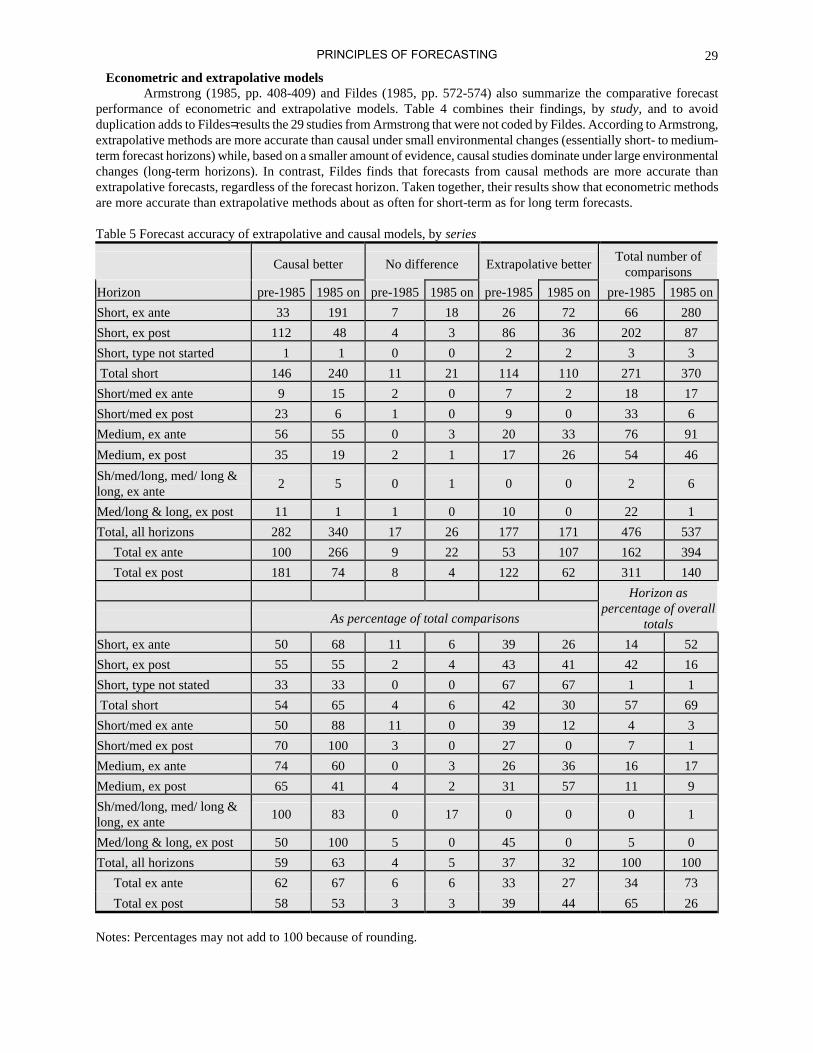
PRINCIPLES OF FORECASTING
29
Econometric and extrapolative models Armstrong (1985, pp. 408-409) and Fildes (1985, pp. 572-574) also summarize the comparative forecast
performance of econometric and extrapolative models. Table 4 combines their findings, by study, and to avoid duplication adds to Fildes= results the 29 studies from Armstrong that were not coded by Fildes. According to Armstrong, extrapolative methods are more accurate than causal under small environmental changes (essentially short- to medium-term forecast horizons) while, based on a smaller amount of evidence, causal studies dominate under large environmental changes (long-term horizons). In contrast, Fildes finds that forecasts from causal methods are more accurate than extrapolative forecasts, regardless of the forecast horizon. Taken together, their results show that econometric methods are more accurate than extrapolative methods about as often for short-term as for long term forecasts. Table 5 Forecast accuracy of extrapolative and causal models, by series
Causal better
No difference
Extrapolative better
Total number of
comparisons Horizon
pre-1985
1985 on
pre-1985
1985 on
pre-1985
1985 on
pre-1985
1985 on
Short, ex ante
33
191
7
18
26
72
66
280 Short, ex post
112
48
4
3
86
36
202
87
Short, type not started
1
1
0
0
2
2
3
3 Total short
146
240
11
21
114
110
271
370
Short/med ex ante
9
15
2
0
7
2
18
17 Short/med ex post
23
6
1
0
9
0
33
6
Medium, ex ante
56
55
0
3
20
33
76
91 Medium, ex post
35
19
2
1
17
26
54
46
Sh/med/long, med/ long & long, ex ante
2
5
0
1
0
0
2
6
Med/long & long, ex post
11
1
1
0
10
0
22
1
Total, all horizons
282
340
17
26
177
171
476
537 Total ex ante
100
266
9
22
53
107
162
394
Total ex post
181
74
8
4
122
62
311
140
As percentage of total comparisons
Horizon as
percentage of overall totals
Short, ex ante
50
68
11
6
39
26
14
52 Short, ex post
55
55
2
4
43
41
42
16
Short, type not stated
33
33
0
0
67
67
1
1 Total short
54
65
4
6
42
30
57
69
Short/med ex ante
50
88
11
0
39
12
4
3 Short/med ex post
70
100
3
0
27
0
7
1
Medium, ex ante
74
60
0
3
26
36
16
17 Medium, ex post
65
41
4
2
31
57
11
9
Sh/med/long, med/ long & long, ex ante
100
83
0
17
0
0
0
1
Med/long & long, ex post
50
100
5
0
45
0
5
0
Total, all horizons
59
63
4
5
37
32
100
100 Total ex ante
62
67
6
6
33
27
34
73
Total ex post
58
53
3
3
39
44
65
26 Notes: Percentages may not add to 100 because of rounding.

ECONOMETRIC FORECASTING 30
Horizons: short: 1 year, 1-6 quarters, or 1-12 months; medium: 2-3 years, 7-12 quarters, or 13-36 months; long: everything else. Sources: Appendix Tables A4-A7. Ex post forecasts should do better in comparative studies than ex ante forecasts, because they use more information. Both Armstrong and Fildes appeared to find contrary evidence and the detailed results by series in Table 5 appear to lend further support to their findings. In each case, the accuracy of ex ante forecasts against their competing extrapolative models was better than the accuracy of ex post forecasts against their competing models. But if the comparison is restricted to the seven studies in Fildes= table 3 (pp. 572-574) in which researchers made both ex ante and ex post forecasts, the expected result occurs. Causal models forecast than extrapolative methods in 48 out of 56 ex post forecast comparisons, but in only 29 out of 56 ex ante forecast comparisons.
We unearthed few other reviews of comparative forecast performance. Table 5 summarizes three surveys by series: Allen (1994, Table 7, agricultural commodities), Fildes (1985, Table 3, mainly macroeconomic series) and Witt and Witt (1985, Table 3, tourism). To these we added comparisons from other studies that reported relative accuracy of out-of-sample forecasts. Detailed list of the individual studies will be found in Appendix Tables A5-A7. Overall, econometric forecasts are more accurate than extrapolative, although the difference is not great, considering that some of the extrapolative forecasts are naive no-change forecasts. Neither is the improvement since 1985 from 59 percent to 64 percent as dramatic as we might have hoped in light of the apparent improvements to both data and econometric methodology.
There is some evidence that at longer horizons the relative performance of econometric methods improves. And again, surprisingly, ex ante econometric forecasts are relatively more successful than ex post forecasts, both before and after 1985. We do not find compelling the theory that this unexpected result arises because forecasted explanatory variables are closer to their long-term means, smoothing out some of the extreme forecasts that result from using actual values of explanatory variables. Rather, we speculate that when additional studies that report both ex ante and ex post forecasts are analyzed, the expected relative strength of ex post forecasts will reappear. A quite reasonable explanation of the findings in Table 5 is that the better model specifications are used mainly for ex ante forecasts, while the poorer specifications are used mainly for ex post forecasts. Table 6 contains some support for this argument. Table 6: Econometric versus univariate forecasts, recorded as (better, no difference, or worse) according to the specified accuracy criterion, by series, with number of studies in parentheses.
Classical single
equation
VAR
Structural sector
model
All econometric
Pre-1985 against Naive
18,2,11 (15)
49,6,15 (8)
67,8,26 (23) ARIMA
53,4,35 (37)
4,0,4 (2)
65,4,64 (15)
122,8,103 (54)
All univariate Better as percent of total
71,6,46 (52)
58
4,0,4 (2)
50
114,10,79 (23)
56
189,16,129 (77)
57 1985 on against Naive
27,4,25 (15)
18,2,5 (6)
45,6,30 (21) ARIMA
29,8,31 (24)
171,8,39 (38)
77,6,46 (9)
276,22,116 (70)
All univariate Better as percent of total
56,12,56 (39)
45
189,10,44 (44)
78
77,6,46 (9)
59
321,28,146 (91)
65
Most forecasts are one-step ahead and RMSE is the usual accuracy criterion. Sources:

PRINCIPLES OF FORECASTING
31
(1) Fildes (1985, Table 3, pp. 572-574), excluding comparisons from three studies that are in Appendix Table A5. For eight studies that reported both ex post and ex ante forecasts, only ex ante results are included here. Together these two exclusions resulted in the omission of (92,1,45) in comparison with Appendix Table A4. (2) Appendix Table 5, using only the ex ante forecasts for two studies that provided both ex ante and ex post forecasts, omitting (3,0,2) in comparison with the detailed table. (3) Appendix Table A6, where using only the ex ante forecasts for one study that provided both ex ante and ex post forecasts, omitting (2,0,2) in comparison with the detailed table. (4) Appendix Table A7,where using only the ex ante forecasts for four studies that provided both ex ante and ex post forecasts, omitting (25,0,25) in comparison with the detailed table.
Table 6 reports the relative forecast accuracy, both before 1985 and since, for various types of econometric models. The division in time is arbitrary, but the later period corresponds to the time since Fildes (1985) survey. It also marks the period when VAR models became popular. Although the benchmarks are divided into naive no-change methods and ARIMA (and extrapolative) methods, the choice of benchmark seems to make little difference. What is noticeable is the rise in the number of VAR models since 1985 and their relatively strong forecast performance compared with classical single-equation models and structural equation systems. A small proportion of the single-equation models were developed using the techniques described in this chapter, but overall, their performance has worsened since 1985. The performance of large-scale structural models is no worse than the forecasting performance of single-equation models, probably because of the advantage with ex post forecasting of using actual explanatory-variable values to keep the system on track. All but a handful of the 245 VAR comparisons are ex ante forecasts, whereas two-thirds of the structural and single-equation comparisons are ex post. Not only are VAR forecasts more accurate, they are more frequently made under more difficult ex ante conditions. RECOMMENDATIONS FOR PRACTITIONERS
What the evidence discussed in this paper does show is that an equation, and if necessary a system of equations, whose explanatory variables are lagged values of the dependent variable and other causal variablesCa vector autoregression modelCis a good starting point. A general-to-specific approach, starting with a large number of lags, will lead to a good, simpler forecasting model. Choice of variables to include in the equation or system is undoubtedly important, and theory should be the predominant guide. Beyond that general suggestion and the advice to keep the model simple, we have no advice about how to pick variables, nor how many to pick, nor have we evidence on the importance of the selection.
Estimate the equation or equations in levels. Ordinary least squares regression is adequate. Ideally, test the residuals of this general model to ensure that they are white noise. If not, the initial model has omitted variables, which should be searched for. Simplify the model by reducing the number of lags. Reducing the lag order on all variables simultanously using likelihood ratio tests is the common first-stage strategy. Reducing the order of individual variables one at a time after putting them in order of importance (Hsiao=s method) is the most usual follow-up, but we have insufficient evidence to compare different simplification methods. Choose the final model on the basis of within-sample fit. Any of the criteria that measure goodness of fit while penalizing excess parameters (AIC, Schwartz BIC) will be good guides. Ideally, the residuals of the simplified model will still be white noise.
As an alternative to the second-stage simplification through lag-order reduction, others suggest performing unit root and cointegration pretests to see if simplification is possible through the introduction of parameter restrictions in the form of cointegration vectors. The tests will also give you additional information about the patterns of the variables and of their relationships to each other over time. If the tests clearly support the existence of one or more cointegrating relations, introduce error-correction restrictions into the simplified model. Less is probably better than more. If cointegration is not clearly indicated, it is probably better to stick with the previous equation.
Less common is further simplification both by reducing lag order and by introducing cointegrating vectors. This brings us back to classical econometrics, since the issue of identification (obtaining a unique set of coefficient estimates) arises here too. If the choice is to simplify either by reducing the lag order on individual variables, or by imposing cointegration restrictions where appropriate, we have insufficient empirical evidence to say which is the better option. Finally, reserve some data to measure out-of-sample forecast performance of the chosen model. If you follow the steps just described, your model should be better than a univariate benchmark. But at this point there are no guarantees. We still have a lot to learn about the usefulness of the various tests in selecting a good forecasting model.

ECONOMETRIC FORECASTING 32
RECOMMENDATIONS FOR RESEARCHERS Improvements in econometric forecasts seem distressingly small and slow to grow. But there are grounds for
optimism because better modeling approaches are emerging. (1) Out-of-sample tests are being more widely used and reported. Ex ante forecasts are appearing more frequently relative to ex post forecasts that use actual values of explanatory variables. Using the information in Table 5, we can see the size of the change. In the earlier years, 52 percent of the forecasts were ex ante. After 1985, in a decided shift, 74 percent of the forecasts were ex ante (2) There has been a shift towards VAR models, and it has paid off in improvement in relative accuracy. The proportion of VAR studies has risen from about three percent before 1985 to almost 50 percent since 1985 (Table 5). VAR forecasts are more accurate against a univariate benchmark than are the forecasts from traditional econometric models. The difference is substantial. But we must note a few cautions. (1) There are some biases in the comparisons. Where several econometric models were estimated, the best performer was compared with the best univariate. Often there was only a solitary univariate competitor. (2) While the forecasting power of VAR models seems clear, there are many unresolved issues. Sometimes unrestricted models outperform more parsimonious models. (Unrestricted models are usually the result of testing an initial model with many lags.) The apparent superiority of Bayesian VARs over standard VARs estimated by OLS hinges on only a few studies. Of greater concern is the poor performance of ECM and VECM models in situations where imposition of the necessary parameter restrictions seems appropriate. Perhaps we await more evidence on the performance of error correction models. (3) We have limited understanding of the role of within-sample specification and misspecification tests. This is a
major impediment to further improvement in econometric forecasts. There is a large and growing literature on the various tests, but it has focused on technical statistical issues that say nothing about how failing a particular test affects forecast performance. Evidence on this vital question is in exceedingly short supply. Does developing an equation with the aid of a battery of tests lead to a version with better forecasting ability? Probably yes. Can we show this? No, or more optimistically, not yet. Which of the tests are important aids to improving forecast performance and which can be ignored? We do not know. What we discover under the well-controlled environment of a Monte Carlo experiment does not always (often?) seem to apply to real data series.
CONCLUSIONS A well-specified econometric model should forecast at least as well as the naive no-change method. The same is true of a well-specified ARIMA model, since the random walk is a special case of each of them. These statements are subject to the usual statistical caveat that there is a controllable chance, the level of significance, where the opposite result will occur. Unfortunately, both econometric and ARIMA models have been beaten by the baseline naive method more often than they should. The inevitable conclusion is that such models do not meet the criterion of Awell specified.@ If all forecasters follow the correct strategy and adopt the correct principles of model building, then only well-specified models will result. The problem is that we are some way from knowing the correct strategy and principles, although we do seem to be making progress.
The principles we developed by examining the literature have been sprinkled through the paper. They are collected and summarized below. We feel confident about some of them: keeping models sophisticatedly simple and comparing out-of-sample performance against a baseline yardstick seem both sound advice and widely accepted principles. We are less confident about other principles, and we would happily see them demolished or refined. Even the answer to the seemingly straightforward question of whether to initially estimate with variables in levels or in differences turns out to be unclear. We still believe in the value of testing. But there is next to no evidence on the value of the tests in improving forecasts of real data series. We even suspect that existing tests, arbitrarily applied, might lead to model specifications with worse forecasting performance.
For the present, we urge practitioners to follow the principles laid down here. But there is clearly much still to be learned, and we urge researchers to use both Monte Carlo experimentation and real data series to help refine the conditions under which the principles operate. Summary of principles of econometric forecasting Principle: Aim for a relatively simple model specification. Conditions: Always Evidence: Monte Carlo (Gilbert 1995). Unrestricted vs. restricted VARs (Table 1)

PRINCIPLES OF FORECASTING
33
Principle: If explanation, including strategy analysis or policy analysis, is the purpose, then make conditional forecasts based on different values of control variables Conditions: When the decision maker can influence the values of the causal variables (e.g., advertising expenditures) but not the parametric relation between cause-and-effect variables. Evidence: Lucas critique (Lucas 1976) Principle: If pure forecasting is the purpose, you must be able to forecast explanatory variables sufficiently well to include them in a forecasting model Conditions: If the MSE of the forecast of the causal variable exceeds its variance, then including the forecasted causal variable will give worse forecasts than omitting it Evidence: Ashley (1983) Principle: Consider all important causal variables based on guidelines from theory and earlier empirical research. Include difficult-to-measure variables and proxy variables. Conditions: Always. Important means Aa change has a large effect on the value of the dependent variable (McClosky & Ziliak 1996). Evidence: None, formally. Choice of variable has been shown to matter: Dua & Smyth (1995), Glaser (1954), Vere & Grifffith (1995). Principle: Choose only one operational variable for each conceptual variable considered. In particular, exclude a proxy variable if its coefficient is small (i.e., has small economic consequence), the remaining coefficients are close to their expected values, or another proxy for the same unobserved variable has better within-sample fit. Conditions: Keep a causal variable if and only if (a) a strong causal relationship (b) the causal relationship can be estimated accurately, (c) the causal variable changes substantially over time, and (d) the change in the causal variable can be forecasted accurately. Evidence: (a) Conforms with parsimony principle (b) Armstrong (1985, p.198), Moyer (1977) (c) Otherwise, the variable=s effect is in the constant term (d) Ashley=s theorem (Ashley 1983) Principle: Collect the longest data series possible. Conditions: As long as there are no structural breaks in the model chosen (for fixed parameter models) or to provide better information on structural breaks. Evidence: Hendry (1996) Principle: Take all previous work into account in specifying a preliminary model. Conditions: Always Evidence: Forecast encompassing tests: Fair & Schiller (1990), Nelson (1972) Principle: Use a general-to-specific approach. Conditions: Always Evidence: In favor: Hendry (1979), Kenward (1976). Against: McDonald (1981) Principle: When disaggregated data are available, use them (a) to obtain an aggregate forecast by summation of disaggregate forecasts (a bottom-up strategy) and (b) to obtain a disaggregate forecast directly, instead of distributing an aggregate forecast (a top-down strategy) although for a specific situation trying and comparing strategies is recommended. Conditions: Both spatial aggregation (over regions or products) and temporal (e.g., from quarterly to annual) Evidence: Spatial: Bottom-up is better in 74 percent of series (Dangerfield & Morris1992). See also Collins (1976), Dangerfield & Morris (1988), Dunn, Williams & Spiney (1971), Leeflang & Wittink (1994), Kinney (1971), Foekens. Temporal: Aggregation loses longer-term cycles (Lütkepohl 1987, Rossana & Seater 1995) Principle: When theory provides a guide to functional form, follow it.
ECONOMETRIC FORECASTING 34
Conditions: Always Evidence: Different functions give different conclusions (Burgess 1975), sometimes permit predictions of negative quantities or prices (Just 1993). Function chosen for best fit can give ludicrous results (Belsley 1988). Principle: Initially, estimate fixed parameter models. Conditions: During model development. Evidence: Gives better understanding of causal structure. Many choices of varying parameter approaches, and many are complex to estimate. Forecast comparisons of varying-parameter and fixed-parameter approaches often appear to use inadequate models. Principle: If possible, use a single equation to make forecasts rather than a system of equations. Conditions: (a) Always for one-step ahead (using a reduced-form equation) (b) When the horizon is short enough that actual values of lagged causal variables are available (c) When causal variable forecasts are available from other sources Evidence: (a) All that is needed (b) Common sense (c) Common sense Principle: Initially estimate equations in levels, not in first differences. Conditions: Always Evidence: Monte Carlo studies (Clements & Hendry, 1995; Engle & Yoo, 1987) Conflicting evidence with real data. Seven of 23 series were better with VAR in levels, 16 of 23 series were better with VAR in differences (Clements & Hendry 1995, Hoffman & Rasche 1996, Joutz, Maddala & Trost 1995, Lin & Tsay 1996, Sarantis & Stewart 1995, Zapata & Garcia 1990). Principle: Estimate equations by ordinary least squares. Conditions: Seems especially important in small samples. Evidence: OLS is less sensitive than other estimators to problems, such as multicollinearity, errors in variables or misspecification (Monte Carlo studies, Kennedy 1992, pp. 157-158). In four out of four series, OLS and GLS forecasts hardly differ (Babula 1988, Harris & Leuthold 1985, Roy & Johnson 1974, Soliman 1971). Two-stage LS is slightly better (Naik & Dixon 1986). OLS and LAV give similar results (Monte Carlo studies, Dielman & Rose1994). Principle: Plot, inspect, and test the residuals for unusual values. Conditions: During model development as a misspecification check Evidence: Plot of series and histogram: Diebold (1998 Chapter 3). Formal procedure (Chen & Liu 1993) improves forecasts (Liu & Lin 1991). For a normality test, the D=Agostino K2 test is almost as powerful as the Shapiro-Wilk test and easier to compute (Monte Carlo studies, D=Agostino & Stephens 1986, pp. 403-4). Principle: Test and remove heteroscedasticity and dynamic heteroscedasticity. Conditions: Appears to be more important for higher frequency data. Ideally, find the cause of the heteroscedasticity before removing it. Evidence: Not correcting for heteroscedasticity distorts the level of significance (Monte Carlo study, Thursby 1992). Three of four studies found ARCH specifications improved forecast accuracy. Five of 10 found it improved volatility forecasts. Principle: Test for autocorrelation. Conditions: During model development as misspecification check. Evidence: Correct it by econometric techniques (Kennedy 1992, p.128, based on Monte Carlo studies) Don=t correct for it (Mizon 1995, Monte Carlo study; use general to specific approach instead). Durbin-Watson test is convenient, but the Breusch-Pagan test is better at detecting higher-order autocorrelations (Mizon & Hendry 1980, Monte Carlo study).

PRINCIPLES OF FORECASTING
35
Practically no evidence on forecasting impact: Yokum & Wildt (1987) found some benefits to autocorrelation correction (without testing for its need). Principle: If the date of a structural break is known (e.g., a change in policy, war, redefinition of series), test for parameter constancy with a single heteroscedasticity-corrected (asymptotic) likelihood ratio test, otherwise use a sequence of tests. Conditions: During model development as misspecification check. Evidence: Heteroscedasticity-corrected form of the Chow test (Chow 1960) is best (Thursby 1992, Monte Carlo study comparing 12 tests). No evidence to prefer particular sequential test (Quandt 1960 or Andrews & Ploberger 1994). In 76 monthly macroeconomic series, the Quandt test rejected parameter constancy more often than other tests, but its impact on forecasts is unknown (Stock & Watson 1996). Principle: Reduce the lag length on each variable in a single equation or separately in each equation in a VAR. Conditions: By using Hsiao=s (1978) method, placing variables in order of importance and minimizing a criterion, such as Schwartz BIC or Akaike FPE or AIC, after reducing the common lag length of all variables from an initial starting point, using likelihood ratio or Box-Tiao tests to do so. Evidence In 35 series in nine models, restricted equations were more accurate over various horizons about three-quarters of the time (Bessler & Babula 1987, Fanchon & Wendell 1992, Funke 1990, Kaylen 1988, Kling & Bessler 1985, Liu, Gerlow & Irwin 1994, Park 1990). BIC is better than FPE (Hafer and Sheehan 1989). Principle Test a data series for a unit root using the modified augmented Dickey-Fuller test (ADF-GLS) proposed by Elliott, Rothenberg, and Stock (1996). Conditions: During preliminary data analysis to gain better understanding of the features of the series. During model simplification before testing for cointegrating vectors Evidence: Test has better properties than other tests and is easier to perform than the ADF test. (Monte Carlo studies, Schwert 1989, Stock 1994, Elliott, Rothenberg and Stock 1996). Principle: Model seasonal data with both deterministic and stochastic seasonality. Conditions: Unless seasonal pattern is judged to be highly regular (by examining a plot of the series) Evidence: Mostly univariate. Significant changes in seasonal pattern, 29 of 40 US and international economic series (Canova & Hansen 1995), in energy consumption (Engle, Granger & Hallman 1989), gross domestic product (Hylleberg, Jorgensen & Sorensen 1993), and Japanese consumption and income (Engle, Granger, Hylleberg & Lee 1993). Seasonal dummy variables and regular and seasonal differencing were more accurate than dummy variables alone in two macroeconomic series (Clements & Hendry 1997). Working with seasonally adjusted data is not advisable. Principle: If possible, simplify the initial model to an error correction model. Conditions: When the results of cointegration tests support the appropriate parameter restrictions Evidence: ECM is consistently more accurate than VAR in two-equation systems with one cointegrating vector (Monte Carlo study, Clements & Hendry 1995, similar results in similar study, Engle & Yoo 1987). The incorrect specification of an ECM gave worse forecasts than a VAR in 12 different two-equation models, although the difference was generally insignificant (Bessler and Fuller 1993). But ECM, used when cointegration tests show it should be, forecast only as well as VAR in levels (aggregate of Bessler & Covey 1991, Fanchon & Wendell 1990, Hall, Anderson, & Granger 1992, Joutz, Maddala & Trost 1995, Sarantis & Stewart 1995, Shoesmith 1995) although much better than VAR in differences (19 of 23 series). Principle: Test all models for performance with data not used in estimation, comparing them with baseline extrapolative or judgmental alternatives. Conditions: Always, after finishing with respecifying and reestimating the model Evidence: The low correlation between fit and forecast performance (Fildes & Makridakis 1995). Principle: Adjust forecasts, especially at short horizons, to allow for forecast origin bias. Conditions: Especially when recent structural changes have occurred. The value of doing so otherwise is less clear, particularly if the adjustment is judgmental.
ECONOMETRIC FORECASTING 36
Evidence: Clements & Hendry (1999), Dhrymes & Peristiani (1988), Fildes & Stekler (1999), McNees (1990). References Abadir, K. M., K. Hadri & E. Tzavalis (1999), AThe Influence of VAR Dimensions on Estimator Biases,@ Econometrica, 67, 163-181. Akgiray, V. (1989), AConditional heteroscedasticity in time series of stock returns: evidence and forecasts,@ Journal of Business, 62, 55-80. Alexander, J.C., Jr. (1995), ARefining the degree of earnings surprise: A comparison of statistical and analysts= forecasts,@ Financial Review, 30, 469-506. Allen, P.G. (1994), AEconomic forecasting in agriculture,@ International Journal of Forecasting, 10, 81-135. Andrews, D.W.K. (1993), ATests for parameter instability and structural change with unknown change point,@ Econometrica, 61, 821-856. Andrews, D.W.K. & W. Ploberger (1994), AOptimal tests when a nuisance parameter is present only under the alternative,@ Econometrica, 62, 1383-1414. Armstrong, J.S. (1985), Long-Range Forecasting From Crystal Ball to Computer, 2nd edition. New York: John Wiley & Sons. Armstrong, J.S. & M.C. Grohman (1972), AA comparative study of methods for long-range market forecasting,@ Management Science, 19, 211-221. Artis, M.J. & W. Zhang (1990), ABVAR forecasts for the G-7,@ International Journal of Forecasting, 6, 349-362. Ashley, R. (1983), AOn the usefulness of macroeconomic forecasts as inputs to forecasting models,@ Journal of Forecasting, 2, 211-223. Ashley, R. (1988), AOn the relative worth of recent macroeconomic forecasts,@ International Journal of Forecasting, 4, 363-376. Babula, R.A. (1988), AContemporaneous correlation and modeling Canada=s imports of U.S. crops,@ Journal of Agricultural Economics Research, 41, 33-38. Banerjee, A., J.J. Dolado, J.W. Galbraith, & D.F. Hendry (1993), Co-integration, error-correction, and the econometric analysis of non-stationary data, Oxford, Oxford University Press. Barrett, C.B. (1997), AHeteroscedastic price forecasting for food security management in developing countries,@ Oxford Development Studies, 25, 225-36. Batchelor, R. & P. Dua (1993), ASurvey vs ARCH measures of inflation uncertainty,@ Oxford Bulletin of Economics & Statistics, 55, 341-53. Belsley, D.A. (1988), AModelling and forecast reliability,@ International Journal of Forecasting, 4, 427-447. Bera, A. & M.L. Higgins (1997), AARCH and bilinearity as competing models for nonlinear dependence,@ Journal of Business & Economic Statistics, 15, 43-50. Bessler, D.A. & R.A. Babula, (1987), AForecasting wheat exports: Do exchange rates matter?@ Journal of Business and Economic Statistics, 5, 397-406. Bessler, D.A. & T. Covey (1991), ACointegration: Some results on U.S. cattle prices,@ Journal of Futures Markets, 11, 461-474.

PRINCIPLES OF FORECASTING
37
Bessler, D.A. & S.W. Fuller (1993), ACointegration between U.S. wheat markets,@ Journal of Regional Science, 33, 481-501. Bewley, R. & M. Yang (1998), AOn the size and power of system tests for cointegration,@ Review of Economics and Statistics, 80, 675-79. Bottomley, P. & R. Fildes (1998), AThe role of prices in models of innovation diffusion,@ Journal of Forecasting, 17, 539-555. . Brailsford, T.J. & R.W. Faff (1996), AAn evaluation of volatility forecasting techniques,@ Journal of Banking & Finance, 20, 419-38. Breusch, T.S. (1978), ATesting for autocorrelation in dynamic linear models,@ Australian Economic Papers, 17, 334-355. Breusch, T.S. & A.R. Pagan (1979), AA simple test for heteroskedasticity and random coefficient variation,@ Econometrica, 47, 1287-1294. Burgess, D.F. (1975), ADuality theory and pitfalls in the specification of technologies,@ Journal of Econometrics, 3, 105-121. Byron, R.P. & O. Ashenfelter (1995), APredicting the quality of an unborn grange,@ Economic Record, 71, 40-53. Campa, J.M. & P.H.K. Chang (1995), AThe forecasting ability of correlations implied in foreign exchange options,@ Columbia University, PaineWebber Working Paper Series in Money, Economics, and Finance: PW/95/26, 19. Canova, F. & B.E. Hansen (1995), AAre seasonal patterns constant over time? A test for seasonal stability,@ Journal of Business and Economic Statistics, 13, 237-252. Challen, D.W. & A.J. Hagger (1983), Macroeconomic Systems: Construction, Validation and Applications, New York: St. Martin=s Press. Chen, C. & L. Liu (1993), AJoint estimation of model parameters and outlier effects in time series,@ Journal of the American Statistical Association, 88, 284-97. Cheung, Y. & M.D. Chinn (1997), AFurther investigation of the uncertain unit root in GNP,@ Journal of Business and Economic Statistics, 15, 68-73. Chow, G.C. (1960), ATests of equality between sets of coefficients in two linear regressions,@ Econometrica, 28, 591-605. Christou, C., P.A.V.B. Swamy, & G.S. Tavlas (1996), AModelling optimal strategies for the allocation of wealth in multicurrency investments,@ International Journal of Forecasting, 12, 483-93. Clements, M.P. & D.F. Hendry (1995), AForecasting in cointegrated systems,@ Journal of Applied Econometrics, 10, 127-146. Clements, M. P. & D. F. Hendry, (1996), AIntercept corrections and structural change,@ Journal of Applied Econometrics, 11, 475-494. Clements, M.P. & D.F. Hendry (1997), AAn empirical study of seasonal unit roots in forecasting,@ International Journal of Forecasting, 13, 341-355. Clements, M.P. & D.F. Hendry (1999), Forecasting Non-stationary Economic Time Series: The Zeuthen Lectures on Economic Forecasting, Cambridge, Mass: MIT Press.

ECONOMETRIC FORECASTING 38
Collins, D.W. (1976), APredicting earnings with sub-entity data: Some further evidence,@ Journal of Accounting Research, 14, 163-177. Conway, R.K., J. Hrubovcak, & M. LeBlanc, 1990, AA forecast evaluation of capital investment in agriculture,@ International Journal of Forecasting 6, 509-519. Cooley, T.F. & E.C. Prescott (1976), AEstimation in the presence of stochastic parameter variation,@ Econometrica, 44, 167-184. D=Agostino, R.B., A. Belanger, & R.B. D=Agostino, Jr. (1990), AA suggestion for using powerful and informative tests of normality,@ The American Statistician, 44, 316-321. D'Agostino, R. B. & M. A. Stephens (1986), Goodness-of-Fit Techniques, New York: Marcel Dekker. Dangerfield, B., & J.S. Morris (1988), AAn empirical evaluation of top-down and bottom-up forecasting strategies,@ Preceedings of the 1988 meeting of Western Decision Sciences Institute, 322-324. Dangerfield, B.J., & J.S. Morris (1992), ATop-down or bottom-up: Aggregate versus disaggregate extrapolation,@ International Journal of Forecasting, 8, 233-241. Davidson, J.E.H., D.F. Hendry, F. Srba & S. Yeo (1978), AEconometric modelling of the aggregate time-series relationship between consumers= expenditure and income in the United Kingdom,@ Economic Journal, 88, 661-92. Davidson, R., & J.G. MacKinnon (1993), Estimation and Inference in Econometrics, New York: Oxford University Press. Dhrymes, P.J. & S.C. Peristiani (1988), AA comparison of the forecasting performance of WEFA and ARIMA time series methods,@ International Journal of Forecasting, 4, 81-101. Dickey, D.A. & W.A. Fuller (1979), ADistribution of the estimators for autoregressive time series with a unit root,@ Journal of the American Statistical Association, 74, 427-431. Diebold, F.X. (1998), Elements of Forecasting. Cincinnati, Ohio: South-Western College Publishing. Dielman, T.E. & R. Pfaffenberger (1982), ALAV (least absolute value) estimation in linear regression: A review,@ TIMS Studies in the Management Sciences, 19, 31-52. Dielman, T.E. & E.L. Rose (1994), AForecasting in least absolute value regression with autocorrelated errors: A small-sample study,@ International Journal of Forecasting, 10, 539-47. Dixon, B.L. & L.J. Martin (1982), AForecasting U.S. pork production using a random coefficient model,@ American Journal of Agricultural Economics, 64, 530-538. Dolado, J. J., T. Jenkinson & S. Sosvilla-Rivero (1990), ACointegration and unit roots,@ Journal of Economic Surveys, 4, 249-73. Dua, P. & D.J. Smyth (1995), AForecasting US home sales using BVAR models and survey data on households= buying attitudes for homes,@ Journal of Forecasting, 14, 217-227. Dunn, D.W., W.H. Williams, & W.A. Spiney (1971), AAnalysis and prediction of telephone demand in local geographic areas,@ Bell Journal of Economics and Management Science, 2, 561-576. Durbin, J. (1970), ATesting for serial correlation in least squares regression when some of the regressors are lagged dependent variables,@ Econometrica, 38, 410-421. Durbin, J. & G.S. Watson (1950), ATesting for serial correlation in least squares regression I,@ Biometrika, 37, 409-428.

PRINCIPLES OF FORECASTING
39
Durbin, J. & G.S. Watson (1951), ATesting for serial correlation in least squares regression II,@ Biometrika, 38, 159-178. Efron, B. (1990), AMore efficient bootstrap computations,@ American Statistician, 85, 79-89. Elliott, G., T.J. Rothenberg, & J.H. Stock (1996), AEfficient tests for an autoregressive unit root,@ Econometrica, 64, 813-836. Engle, R.F. (1982), AAutoregressive conditional heteroskedasticity with estimates of the variance of United Kingdom inflation,@ Econometrica, 50, 987-1007. Engle, R.F., S.J. Brown, & G. Stern (1988), AA comparison of adaptive structural forecasting methods for electricity sales,@ Journal of Forecasting, 7, 149-172. Engle, R.F. & C.W.J. Granger (1987), ACo-integration and error correction: Representation, estimation, and testing,@ Econometrica, 55, 251-276. Engle, R.F., C.W.J. Granger, & J.J. Hallman (1989), AMerging short- and long-run forecasts,@ Journal of Econometrics, 40, 45-62. Engle, R.F., C.W.J. Granger, S. Hylleberg & H. Lee (1993), ASeasonal cointegration: the Japanese consumption function,@ Journal of Econometrics, 55, 275-298. Engle, R.F., D.F. Hendry, & D. Trumble (1985), Small-sample properties of ARCH estimators and tests,@ Canadian Journal of Economics, 18, 66-93. Engle, R.F. & B.S. Yoo (1987), AForecasting and testing in co-integrated systems,@ Journal of Econometrics, 35, 143-159. Fair, R.C. & R.J. Shiller, 1990, AComparing information in forecasts from econometric models,@ American Economic Review, 80, 375-89. Fanchon, P. & J. Wendell (1992), AEstimating VAR models under non-stationarity and cointegration: Alternative approaches to forecasting cattle prices,@ Applied Economics, 24, 207-217. Figlewski, S. (1994), AForecasting volatility using historical data,@ New York University Salomon Brothers Working Paper: S-94-13, 29. Fildes, R. (1985), AQuantitative forecasting - the state of the art: Econometric models,@ Journal of the Operational Research Society, 36, 549-580. Fildes, R. & S. Makridakis (1995), AThe impact of empirical accuracy studies on time series analysis and forecasting,@ International Statistical Review, 63, 289-308. Fildes, R. & H. Stekler (1999), AThe state of macroeconomic forecasting,@ Working Paper 99/1, Department of Management Science, Lancaster University, UK. Foekens, E.W., P.S.H. Leeflang & D.R. Wittink (1994), AA comparison and an exploration of the forecasting accuracy of a loglinear model at different levels of aggregation,@ International Journal of Forecasting, 10, 245-261. Frennberg, P. & B. Hansson (1995), AAn evaluation of alternative models for predicting stock volatility: Evidence from a small stock market,@ Journal of International Financial Markets, Institutions & Money, 5, 117-34. Funke, M. (1990), AAssessing the forecasting accuracy of monthly vector autoregressive models: The case of five OECD Countries,@ International Journal of Forecasting, 6, 363-78.

ECONOMETRIC FORECASTING 40
Garcia-Ferrer, A., R.A. Highfield, F. Palm, & A. Zellner (1987), AMacroeconomic forecasting using pooled international data,@ Journal of Business & Economic Statistics, 5, 53-67. Gilbert, P.D. (1995), ACombining VAR estimation and state space model reduction for simple good predictions,@ Journal of Forecasting, 14, 229-250. Glaser, D. (1954), AA reconsideration of some parole prediction factors,@ American Sociological Review, 19, 335-340. Godfrey, L.G. (1978), AA diagnostic check of the variance model in regression equations with heteroscedastic disturbances,@ Unpublished paper, University of York. Godfrey, L.G. (1988), Misspecification Tests in Econometrics, Cambridge, Cambridge University Press. Gordon, D.V. & W.A. Kerr (1997), AWas the Babson prize deserved? An enquiry into an early forecasting model,@ Economic Modelling, 14, 417-33. Granger, C.W.J. & P. Newbold (1974), ASpurious regressions in econometrics,@ Journal of Econometrics, 2, 111-120. Haavelmo, T. (1944), AThe probability approach in econometrics,@ Econometrica, 12, (Supplement, July, 1944), 1-115. Hafer, R W & R.G. Sheehan (1989), AThe sensitivity of VAR forecasts to alternative lag structures,@ International Journal of Forecasting, 5, 399-408. Hall, A.D., H.M. Anderson & C.W.J. Granger (1992), AA cointegration analysis of Treasury bill yields,@ Review of Economics and Statistics, 74, 116-126. Hannan, E.J. & R.D. Terrell (1966), ATesting for serial correlation after least squares regression,@ Econometrica, 34, 646-660. Harris, K.S. & R.M. Leuthold (1985), AA comparison of alternative forecasting techniques for livestock prices: A case study,@ North Central Journal of Agricultural Economics, 7, 40-50. Hendry, D.F. (1979), A Predictive failure and econometric modelling in macroeconomics: the transactions demand for money,@ Ch. 9, pp. 217-242 in P. Ormerod ed., Economic Modelling, London, Heinemann. Hendry, D.F. (1980), AEconometrics - alchemy or science,@ Economica, 47, 387-406. Hendry, D.F. (1996), AA theory of co-breaking,@ paper presented at the 17th International Symposium of Forecasting, Barbados, W.I., June 19-21, 1997. Hendry, D.F., A.R. Pagan, & J.D. Sargan (1984), ADynamaic specification,@ Ch. 18 in Z. Griliches and M.D. Intriligator eds., Handbook of Econometrics, Vol. 2, Amsterdam, North Holland. Hendry, D.F. & J.-F. and Richard (1982), AOn the formulation of empirical models in dynamic econometrics,@ Journal of Econometrics, 20, 3-33. Hildreth, C., & J.P. Houck (1968), ASome estimators for a linear model with random coefficients,@ Journal of the American Statistical Association, 63, 584-595. Hillmer, S. (1984), AMonitoring and adjusting forecasts in the presence of additive outliers,@ Journal of Forecasting, 3, 205-215. Hoffman, D.L. & R.H. Rasche (1996), AAssessing forecast performance in a cointegrated system,@ Journal of Applied Econometrics, 11, 495-517.

PRINCIPLES OF FORECASTING
41
Holden, K. & A. Broomhead (1990), AAn examination of vector autoregressive forecasts for the U.K. economy,@ International Journal of Forecasting, 6, 11-23. Hopkins, Jr., J.A. (1927), AForecasting cattle prices,@ Journal of Farm Economics, 9, 433-446. Hsiao, C. (1979), AAutoregressive modeling of Canadian money and income data,@ Journal of the American Statistical Association, 74, 553-60. Hylleberg, S., R.F. Engle, C.W.J. Granger, & B.S. Yoo (1990), ASeasonal integration and cointegration,@ Journal of Econometrics, 44, 215-238. Hylleberg, S., C. Jorgensen & N.K. Sorensen (1993), ASeasonality in macroeconomic time series,@ Empirical Economics, 18, 321-335. Inder, B.A. (1984), AFinite-sample power of tests for autocorrelation in models containing lagged dependent variables,@ Economics Letters, 14, 179-185 Jarque, C.M. & A.K. Bera (1980), Efficient tests for normality, heteroskedasticity and serial independence of regression residuals,@ Economics Letters, 6, 255-259. Johansen, S. (1988), AStatistical analysis of cointegrating vectors,@ Journal of Economic Dynamics and Control, 12, 231-254. Johansen, S. & K. Juselius (1990), AMaximum likelihood estimation and inference on cointegration - with applications to the demand for money,@ Oxford Bulletin of Economics and Statistics, 52, 169-210. Joutz, F.L., G.S. Maddala, & R.P. Trost (1995), AAn integrated Bayesian vector autoregression and error correction model for forecasting electricity consumption and prices,@ Journal of Forecasting, 14, 287-310. Judge, G.G., R.C. Hill, W.E. Griffiths, H. Lütkepohl, & T.-C. Lee (1985), The Theory and Practice of Econometrics, second edition. New York: John Wiley & Sons. Just, R. E. (1993), ADiscovering production and supply relationships: present status and future opportunities,@ Review of Marketing and Agricultural Economics, 61, 11-40. Kaylen, M.S. (1988), AVector autoregression forecasting models: Recent developments applied to the U.S. hog market,@ American Journal of Agricultural Economics, 70, 701-712. Kennedy, P. (1992), A Guide to Econometrics. Cambridge, Massachusetts: The MIT Press. Kenward, L. R. (1976), AForecasting quarterly business expenditures on non-residential construction in Canada: An assessment of alternative models,@ Canadian Journal of Economics, 9, 517-529. King, M.L. (1987), ATesting for autocorrelation in linear regression models: A survey,@ Ch. 3 in M. King and D. Giles (eds.), Specification Analysis in the Linear Model. London: Routledge and Kegan Paul. Kinney, W.R. Jr. (1971), APredicting earnings: Entity vs. sub-entity data,@ Journal of Accounting Research, 9, 127-136. Kiviet, J.F. (1986), AOn the rigour of some misspecification tests for modelling dynamic relationships,@ Review of Economic Studies, 53, 241-261. Kling, J.L. & D.A. Bessler (1985), AA comparison of multivariate forecasting procedures for economic time series,@ International Journal of Forecasting, 1, 5-24. Koenker, R. (1988), AAsymptotic Theory and Econometric Practice,@ Journal of Applied Econometrics, 3, 139-147.

ECONOMETRIC FORECASTING 42
Kramer, W., H. Sonnberger, J. Maurer & P. Havlik (1985), ADiagnostic checking in practice,@ Review of Economics and Statistics, 67, 118-123. Leamer, E.E. (1983), ALet=s take the con out of econometrics,@ American Economic Review, 73, 31-43. Ledolter, J. (1989), AThe effect of additive outliers on the forecasts from ARIMA models,@ International Journal of Forecasting, 5, 231-240. Lin, J-L. & R.S. Tsay (1996), ACo-integration constraint and forecasting: an empirical examination,@ Journal of Applied Econometrics, 11, 519-538. Liu, L. & M. Lin (1991), AForecasting residential consumption of natural gas using monthly and quarterly time series,@ International Journal of Forecasting, 7, 3-16. Liu, T-R., M.E. Gerlow & S.H. Irwin (1994), The performance of alternative VAR models in forecasting exchange rates,@ International Journal of Forecasting, 10, 419-433. Lucas, R.E., Jr. (1976), AEconometric policy evaluation: a critique,@ in K. Brunner and A.H. Meltzer, The Phillips Curve and Labor Markets, Carnegie-Rochester Conference Series on Public Policy, 1, North-Holland, Amsterdam, 19-46. Lütkepohl, H (1987),. Forecasting aggregated vector ARMA processes. Lecture Notes in Economics and Mathematical Systems series, no. 284. New York; Berlin; London and Tokyo: Springer. Lütkepohl, H. (1991), Introduction to Multiple Time Series Analysis, New York, Springer-Verlag. MacKinnon, J.G. (1991), ACritical values for cointegration tests,@ Ch. 13 in R.F. Engle and C.W.J. Granger eds., Long-run Economic Relationships: Readings in Cointegration, Oxford, Oxford University Press. Maddala, G.S. (1988), Introduction to Econometrics. New York: Macmillan. Mayer, T. (1975), ASelecting economic hypotheses by goodness of fit,@ Economic Journal, 85, 877-883. Mayer, T. (1980), AEconomics as a hard science: Realistic goal or wishful thinking?@ Economic Inquiry, 18, 165-178. McCloskey, D.N. & S.T. Ziliak (1996), AThe standard error of regressions,@ Journal of Economic Literature, 34, 97-114. McCurdy, T.H. & T. Stengos (1991), AA comparison of risk-premium forecasts implied by parametric versus nonparametric conditional mean estimators,@ Queen's Institute for Economic Research Discussion Paper: 843, 25. McDonald, J. (1981), AModelling demographic relationships: An analysis of forecast functions for Australian births, with discussion,@ Journal of the American Statistical Association, 76, 782-801. McNees, S.K. (1990), AThe role of judgment in macroeconomic forecasting accuracy,@ International Journal of Forecasting, 6, 287-288. Mizon, G.E. (1995), AA simple message for autocorrelation correctors: Don=t,@ Journal of Econometrics, 69, 267-288. Mizon, G.E. & D.F. Hendry (1980), AAn empirical and Monte Carlo analysis of tests of dynamic specification,@ Review of Economic Studies, 47, 21-45. Mizon, G.E. & J.-F. Richard (1986), AThe encompassing principle and its application to testing non-nested hypotheses,@ Econometrica, 54, 657-678. Moyer, R.C. (1977), AForecasting financial failure: A re-examination,@ Financial Management, 6, 11-17.

PRINCIPLES OF FORECASTING
43
Murray, M. P. (1994), AA drunk and her dog: an illustration of cointegration and error correction,@ American Statistician, 48, 37-39. Myers, R.J. & S.D. Hanson (1993), APricing commodity options when the underlying futures price exhibits time-varying volatility,@ American Journal of Agricultural Economics, 75, 121-30. Naik, G. & B.L. Dixon (1986), AA Monte-Carlo comparison of alternative estimators of autocorrelated simultaneous systems using a U.S. pork sector model as the true structure,@ Western Journal of Agricultural Economics, 11, 134-145. Nelson, C.R. (1972), AThe prediction performance of the FRB-MIT-PENN model of the U.S. economy,@ American Economic Review, 62, 902-17. Neter, J., M.H. Kutner, C.J. Nachtsheim & W. Wasserman (1996), Applied Linear Statistical Models, 4th ed. Chicago: Irwin. Noh, J., R.F. Engle, & A. Kane (1993), AA test of efficiency for the S&P 500 index option market using variance forecasts,@ University of California, San Diego Department of Economics Working Paper: 93-32, 25. Osterwald-Lenum, M. (1992), AA note with quantiles of the asymptotic distribution of the maximum likelihood cointegration rank test statistics,@ Oxford Bulletin of Economics and Statistics, 54, 461-472. Park, T. (1990), AForecast evaluation for multivariate time-series models: The U.S. cattle market,@ Western Journal of Agricultural Economics, 15, 133-143. Peach, J.T. & J.L. Webb (1983), ARandomly specified macroeconomic models: Some implications for model selection, Journal of Economic Issues, 17, 697-720. Quandt, R.E. (1960), ATests of the hypothesis that a linear regression system obeys two separate regimes,@ Journal of the American Statistical Association, 55, 324-330. Riddington, G.L. (1993), ATime varying coefficient models and their forecasting performance,@ OMEGA , 21, 573-583. Rippe, R.D. & M. Wilkinson (1974), AForecasting accuracy of the McGraw-Hill anticipations data,@ Journal of the American Statistical Association, 69, 849-858. Rossana, R. J. & J. J. Seater (1995), ATemporal aggregation and economic time series@, Journal of Business and Economic Statistics, 13, 441B451. Roy, S.K. & P.N. Johnson (1974), Econometric Models of Cash and Futures Prices of Shell Eggs. USDA-ERS Technical Bulletin Number 1502, 32pp. Sarantis, N. & C. Stewart (1995), AStructural, VAR and BVAR models of exchange rate determination: A comparison of their forecasting performance@, Journal of Forecasting, 14, 201-215. Sarle, C. F. (1925), AThe forecasting of the price of hogs,@ American Economic Review, 15, Number 3, Supplement Number 2, 1-22. Sarmiento, C. (1996), AComparing two modeling approaches: An example of fed beef supply,@ MS Thesis, University of Massachusetts.. Schwert, G. W. (1989), ATests for unit roots: A Monte Carlo investigation,@ Journal of Business and Economic Statistics, 7, 147-159. Shapiro, S.S. & M.B. Wilk (1965), AAn analysis of variance test for normality (complete samples),@ Biometrika, 52, 591-611.

ECONOMETRIC FORECASTING 44
Shoesmith, G.L. (1995), AMultiple cointegrating vectors, error correction, and forecasting with Litterman's model,@ International Journal of Forecasting, 11, 557-67. Sims, C. A., J. H. Stock & M. W. Watson (1990), AInference in linear time series models with some unit roots,@ Econometrica., 58, 113-144. Soliman, M.A. (1971), AEconometric model of the turkey industry in the United States,@ Canadian Journal of Agricultural Economics 19, 47-60. Sowey, E.R. (1973), AA classified bibliography of Monte Carlo studies in econometrics,@ Journal of Econometrics, 1, 377-395. Spanos, A. (1995), AOn theory testing in econometrics: Modeling with nonexperimental data,@ Journal of Econometrics, 67, 189-226. Spencer, D.E. (1993), ADeveloping a Bayesian vector autoregression forecasting model,@ International Journal of Forecasting, 9, 407-421. Stock, J.H. (1994), AUnit roots, structural breaks and trends,@ Handbook of Econometrics, Vol. 4, Chapter 46, 2739-2841. Stock, J.H. & M.W. Watson (1996), AEvidence on structural instability in macroeconomic time series relations,@ Journal of Business and Economic Statistics, 14, 11-30. Swamy, P.A.V.B., R.K. Conway, & M.R. LeBlanc (1989), AThe stochastic coefficients approach to econometric modeling, part III: Estimation, stability testing and prediction,@ Journal of Agricultural Economics Research, 41, 4-20. Swamy, P.A.V.B., A.B. Kennickell, & P. von zur Muehlen (1990), AComparing forecasts from fixed and variable coefficient models: the case of money demand,@ International Journal of Forecasting, 6, 469-477. Swamy, P.A.V.B., & P.A. Tinsley (1980), ALinear prediction and estimation methods for regression models with stationary stochastic coefficients,@ Journal of Econometrics, 12, 103-142. Thursby, J.G. (1992), AA comparison of several exact and approximate tests for structural shift under heteroscedasticity,@ Journal of Econometrics, 53, 363-386. Vere, D.J. & G.R. Griffith (1995), AForecasting in the Australian Lamb industry: The influence of alternative price determination processes,@ Review of Marketing and Agricultural Economics, 63, 408-18. West, K.D. & D. Cho (1995), AThe predictive ability of several models of exchange rate volatility,@ Journal of Econometrics, 69, 367-91. Witt, S. F. & C.A. Witt (1995), AForecasting tourism demand: A review of empirical research,@ International Journal of Forecasting, 11, 447-75. Yokum, J.T., Jr., & A.R. Wildt (1987), AForecasting sales response for multiple time horizons and temporally aggregated data,@ International Journal of Forecasting, 3, 479-488. Zapata, H.O. & P. Garcia (1990), APrice forecasting with time-series methods and nonstationary data: An application to monthly U.S. cattle prices,@ Western Journal of Agricultural Economics, 15, 123-132.

PRINCIPLES OF FORECASTING
45
Biographies Geoff Allen has been surrounded by forecasters all his life, though he generally did not realize it at the time. An
early introduction to probability forecasting was provided by his mother, whose principles (Astay away from that cliff or you=ll hurt yourself@) were sometimes ignored and occasionally true.
He received a bachelors degree from the University of Nottingham, where he did not meet Clive Granger, and a Ph.D. in agricultural economics from the University of California, where he missed a second opportunity to meet Clive Granger. But he did meet Robert Fildes.
Years later, while on sabbatic leave he visited Robert Fildes and was persuaded to take a vacation to Istanbul where there happened to be a forecasting conference (the second ISF). There he met Scott Armstrong. It would be nice to record that this marked the start of his forecasting career (though he did not realize it at the time) and the rest, as they say, is history. Nice but not necessarily true. He spent many years working in economics on a variety of topics: environmental policy, aquaculture-production decisions and agricultural risk management, before realizing that most of these are in some way connected with forecasting.
Robert Fildes started his academic life as a mathematician and applied probabilist, first at Oxford and subsequently at the University of California, Davis. His collaborations with Geoff Allen were at that time reserved for planning skiing trips. After exhausting his interest in theoretical mathematics, he accepted a post at the Manchester Business School, meeting a career goal to work in one of Britain's newly founded business schools and returning him to his home town. Following an exhortation to 'do something useful' in management science, he found himself teaching and researching forecasting.
A well-received first book on forecasting led Spyros Makridakis to co-opt him to write a chapter for the TIMS Studies in Management Science on selecting forecasting methods. It required a lot of reading, so putting to work the management-efficiency concepts that were being taught all around him, he collected the references into a bibliography. Eventually, this turned into two publications listing 7,000 of the major forecasting papers for the years 1965-1981. In an attempt to deflect the scorn of his academic colleagues and to rise above this exercise in mere cataloging, he wrote two survey papers (published in 1979 and 1985 in the Journal of the Operational Research Society (1985) summarizing the effectiveness of extrapolative and causal forecasting methods respectively. The latter paper is the progenitor of the more ambitious set of econometric principals laid out here.
But survey papers take a lot of work and are not always thought to demonstrate the highest levels of intellect. Despite (or even because of) the ambition of the forecasting principles project and because of prior commitments, he turned down Scott Armstrong's request to contribute a chapter on econometric principles. He did agree, though, to collaborate as a third author. Now that the project is completed, the question of the missing second author still haunts him.
In founding the Journal of Forecasting and in l985 the International Journal of Forecasting and later as Editor and Chief Editor of these journals, he has collaborated for long periods with Scott Armstrong and Spyros Makridakis. Both have had a major influence on his thinking. Acknowledgments We thank David Bessler, Ron Bewley, Frank Diebold, David Hendry, Ken Holden, Steve McNees and four anonymous reviewers for their helpful comments on earlier drafts and for their enthusiastic support. Scott Armstrong has been tireless in his efforts to help us avoid obscurity and replace it with clarity. He was ably assisted by Mary Haight. The first author uses econometrics but does not claim to be an econometrician. He is grateful to his colleague Bernie Morzuch (who is one) both for comments on earlier drafts and for many helpful econometric discussions. P. Geoffrey Allen, [email protected] Department of Resource Economics University of Massachusetts Amherst, MA 01003 USA (413) 545-5715, FAX (413) 545-5853 August 26, 1999 (4:38PM) Converted to Word with minor typographic correction, March 13, 2000