efficient mcmc for continuous time discrete state...
TRANSCRIPT

Efficient MCMC for
Continuous Time Discrete State Systems
Vinayak Rao and Yee Whye Teh
Gatsby Computational Neuroscience Unit,University College London

Overview
Continuous time discrete state systems: applications in physics,chemistry, genetics, ecology, neuroscience etc.
The simplest example: the Poisson process on the real line.
Generalizations: renewal processes, Markov jump processes,continuous time Bayesian networks etc.
These relate back to the basic Poisson process via the idea ofuniformization.
We use this connection to develop tractable models and efficientMCMC sampling algorithms.
Vinayak Rao, Yee Whye Teh (Gatsby Unit) MCMC for Continuous Time Systems 2 / 40

ThinningUniformization generalizes the idea of ‘thinning’.
Thinning: to sample from a Poisson process with rate λ(t).
Sample from a Poisson process with rate Ω > λ(t) ∀t.
Thin or reject each point with probability 1− λ(t)Ω
.
o
x
o
o
x
o
Follows from the complete randomness of the Poisson process.
Markov jump processes or renewal processes are not completelyrandom: Uniformization—thin points by running a Markov chain.
Vinayak Rao, Yee Whye Teh (Gatsby Unit) MCMC for Continuous Time Systems 3 / 40
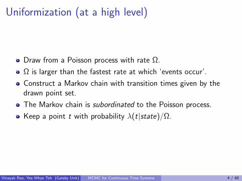
Uniformization (at a high level)
Draw from a Poisson process with rate Ω.
Ω is larger than the fastest rate at which ‘events occur’.
Construct a Markov chain with transition times given by thedrawn point set.
The Markov chain is subordinated to the Poisson process.
Keep a point t with probability λ(t|state)/Ω.
Vinayak Rao, Yee Whye Teh (Gatsby Unit) MCMC for Continuous Time Systems 4 / 40

Markov jump processes (MJPs)
An MJP S(t), t ∈ R+ is a right-continuous piecewise-constantstochastic process taking values in some finite space. S = 1, 2, ...n.It is parametrized by an initial distribution π and a rate matrix A.
A11 A12 . . . A1n
A21 A22 . . . A2n...
.... . .
...An1 An2 . . . Ann
Aij : rate of leaving state i for j
Aii = −n∑
j=1,j 6=i
Aij
|Aii | : rate of leaving state i
Vinayak Rao, Yee Whye Teh (Gatsby Unit) MCMC for Continuous Time Systems 5 / 40

Uniformization for MJPs
Alternative to Gillespie’s algorithm.
Sample a set of times from a Poisson process with rateΩ ≥ maxi |Aii | on the interval [tstart , tend ].
Run a discrete time Markov chain with initial distribution π andtransition matrix B = (I + 1
ΩA) on these times.
The matrix B allows self-transitions.[Jensen, 1953]
Vinayak Rao, Yee Whye Teh (Gatsby Unit) MCMC for Continuous Time Systems 6 / 40
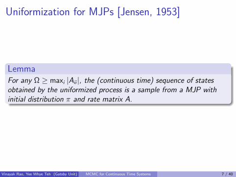
Uniformization for MJPs [Jensen, 1953]
LemmaFor any Ω ≥ maxi |Aii |, the (continuous time) sequence of statesobtained by the uniformized process is a sample from a MJP withinitial distribution π and rate matrix A.
Vinayak Rao, Yee Whye Teh (Gatsby Unit) MCMC for Continuous Time Systems 7 / 40

Auxiliary variable Gibbs sampler
Given noisy observations of an MJP, obtain samples from theposterior.
Observations can include:
State values at the end points of an interval.
Observations x(t) ∼ F (S(t)) at a finite set of times t.
More complicated likelihood functions that depend on the entiretrajectory, e.g. Markov modulated Poisson processes andcontinuous time Bayesian networks (see later).
State space of Gibbs sampler consist of:
Trajectory of MJP S(t).
Auxiliary set of points rejected via self-transitions.
[Rao and Teh, 2011a]
Vinayak Rao, Yee Whye Teh (Gatsby Unit) MCMC for Continuous Time Systems 8 / 40
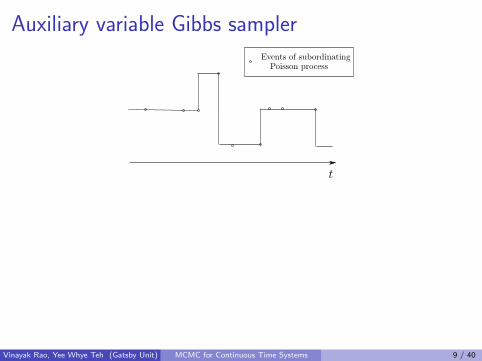
Auxiliary variable Gibbs sampler
Vinayak Rao, Yee Whye Teh (Gatsby Unit) MCMC for Continuous Time Systems 9 / 40

Auxiliary variable Gibbs sampler
Given current MJP path, we need to resample the set of rejectedpoints. Conditioned on the path, these are:
I independent of the observations,I produced by ‘thinning’ a rate Ω Poisson process with probability
1 +AS(t)S(t)
Ω ,I thus, distributed according to a inhomogeneous Poisson process
with piecewise constant rate (Ω + AS(t)S(t)).
Vinayak Rao, Yee Whye Teh (Gatsby Unit) MCMC for Continuous Time Systems 9 / 40

Auxiliary variable Gibbs sampler
Given all potential transition points, the MJP trajectory isresampled using the forward-filtering backward-samplingalgorithm.
The likelihood of the state between 2 successive points mustinclude all observations in that interval.
Vinayak Rao, Yee Whye Teh (Gatsby Unit) MCMC for Continuous Time Systems 9 / 40

Comments
Complexity: O(n2P), where P is the (random) number of points.
Can take advantage of sparsity in transition rate matrix A.
Only dependence between successive samples is via thetransition times of the trajectory.
Increasing Ω reduces this dependence, but increasescomputational cost.
Sampler is ergodic for any Ω > maxi |Aii |.
Vinayak Rao, Yee Whye Teh (Gatsby Unit) MCMC for Continuous Time Systems 10 / 40
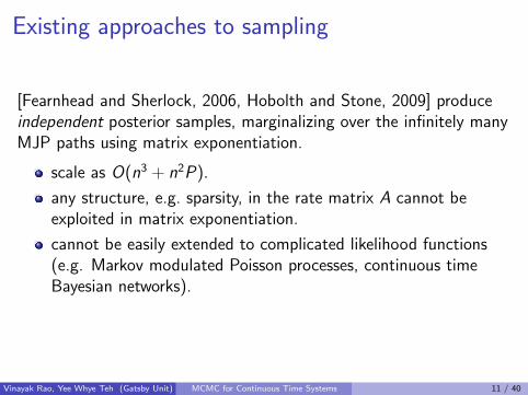
Existing approaches to sampling
[Fearnhead and Sherlock, 2006, Hobolth and Stone, 2009] produceindependent posterior samples, marginalizing over the infinitely manyMJP paths using matrix exponentiation.
scale as O(n3 + n2P).
any structure, e.g. sparsity, in the rate matrix A cannot beexploited in matrix exponentiation.
cannot be easily extended to complicated likelihood functions(e.g. Markov modulated Poisson processes, continuous timeBayesian networks).
Vinayak Rao, Yee Whye Teh (Gatsby Unit) MCMC for Continuous Time Systems 11 / 40

Continuous-time Bayesian networks (CTBNs)
Compact representations of large state space MJPs withstructured rate matrices.
Applications include ecology, chemistry , network intrusiondetection, human computer interaction etc.
The rate matrix of a node at time is determined by theconfiguration of its parents at that time.
[Nodelman et al., 2002]
Vinayak Rao, Yee Whye Teh (Gatsby Unit) MCMC for Continuous Time Systems 12 / 40

Gibbs sampling CTBNs via uniformization
?
NP C
The trajectories of all nodes are piecewise constant.
In a segment of constant parent (P) values, the dynamics of Nare controlled by a fixed rate matrix AP .
Each child (C) trajectory is effectively a continuous-timeobservation.
Vinayak Rao, Yee Whye Teh (Gatsby Unit) MCMC for Continuous Time Systems 13 / 40

Gibbs sampling CTBNs via uniformization
?
NP C
Sample candidate transition times from a Poisson process withrate Ω > AP
ii .
Between two successive Poisson events, N remains in a constantstate.
I This state must account for the likelihood of children nodes’states.
I The state must also explain relevant observations.
With the resulting ‘likelihood’ function and transition matrixB = (I + 1
ΩAP), sample new trajectory using forward-filtering
backward-sampling.
Vinayak Rao, Yee Whye Teh (Gatsby Unit) MCMC for Continuous Time Systems 13 / 40

Existing approaches to inference
[El-Hay et al., 2008] describe a Gibbs sampler involving timediscretization, which is expensive and approximate.
[Fan and Shelton, 2008] uses particle filtering which can beinaccurate for long time intervals.
[Nodelman et al., 2002, Nodelman et al., 2005,Opper and Sanguinetti, 2007, Cohn et al., 2010] use deterministicapproximations (mean-field and expectation propagation) which arebiased and can be inaccurate.
Vinayak Rao, Yee Whye Teh (Gatsby Unit) MCMC for Continuous Time Systems 14 / 40

Experiments
We compare our uniformization-based sampler with astate-of-the-art CTBN Gibbs sampler of [El-Hay et al., 2008].search on the time interval.
When comparing running times, we measured times required toproduce same effective sample sizes.
Vinayak Rao, Yee Whye Teh (Gatsby Unit) MCMC for Continuous Time Systems 15 / 40

Experiments
0 10 20 30 40 5010
−1
100
101
102
103
Number of nodes in CTBN chain
CP
U ti
me
in s
econ
ds
UniformizationEl Hay et al.El Hay et al. (Matrix exp.)
Figure: CPU time vs length ofCTBN chain.
100
101
102
10−2
10−1
100
101
102
103
Dimensionality of nodes in CTBN chain
CP
U ti
me
in s
econ
ds
UniformizationEl Hay et al.El Hay et al. (Matrix exp.)
Figure: CPU time vs numberof states of CTBN nodes.
The plots above were produced for a CTBN with a chain topology,increasing the number of nodes in the chain (left) and the number ofstates of each node (right).
Vinayak Rao, Yee Whye Teh (Gatsby Unit) MCMC for Continuous Time Systems 16 / 40
Experiments
101
102
103
100
101
102
103
104
Length of CTBN time−interval
CP
U ti
me
in s
econ
ds
UniformizationEl Hay et al.El Hay et al. (Matrix exp.)
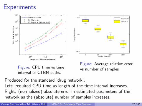
Figure: CPU time vs timeinterval of CTBN paths.
10 100 1000 10000Number of samples
10−1
100
101
Uniformization
El Hay et al.
Ave
rage
Rel
ativ
e E
rror
Figure: Average relative errorvs number of samples
Produced for the standard ‘drug network’.Left: required CPU time as length of the time interval increases.Right: (normalized) absolute error in estimated parameters of thenetwork as the (absolute) number of samples increases.
Vinayak Rao, Yee Whye Teh (Gatsby Unit) MCMC for Continuous Time Systems 17 / 40

Experiments
Compared against the mean-field approximation of[Opper and Sanguinetti, 2007], for the predator-prey model, a CTBNdescribing the Lotka-Volterra equations.
0 500 1000 1500 2000 2500 30000
5
10
15
20
25
30
True path
Mean−field approx.
MCMC approx.
0 500 1000 1500 2000 2500 30000
5
10
15
20
25
30
True path
Mean−field approx.
MCMC approx.
Posterior (mean and 90% confidence intervals) over predator paths(observations (circles) only until 1500).
Vinayak Rao, Yee Whye Teh (Gatsby Unit) MCMC for Continuous Time Systems 18 / 40

Renewal processes
Renewal processes: point processes on the real line (‘time’).
Inter-event times drawn i.i.d. from some renewal density.
Homogeneous Poisson process: exponential renewal density.
Can capture burstiness or refractoriness.
Our contribution: modulated renewal processes:
Nonstationarity: allow external time-varying factors to modulatethe inter-event distribution.
We place a (transformed) Gaussian process prior on the intensityfunction.
[Rao and Teh, 2011b]
Vinayak Rao, Yee Whye Teh (Gatsby Unit) MCMC for Continuous Time Systems 19 / 40

Modulated renewal processes
Associated with the renewal density g is a hazard function h.
For an infinitesimal ∆, h(τ)∆ is the probability of the inter-eventinterval being in [τ, τ + ∆] conditioned on it being at least τ :
h(τ) =g(τ)
1−∫ τ
0g(u)du
Modulate the hazard function by some time-varying intensityfunction λ(t):
h(τ, t) ≡ m(h(τ), λ(t))
m(·, ·) is some interaction function.
We use multiplicative interactions, h(τ, t) = h(τ)λ(t).
Another interaction function is additive h(τ, t) = h(τ) + λ(t).
Vinayak Rao, Yee Whye Teh (Gatsby Unit) MCMC for Continuous Time Systems 20 / 40

Modulated renewal processes (continued)
We place a Gaussian Process prior on the intensity functionλ(t), transformed via a sigmoidal link function.
We use a gamma family for the hazard function:
h(τ) =xγ−1e−x∫∞
xuγ−1e−udu
where γ is the shape parameter. The generative process is:
l(·) ∼ GP(µ,K )
λ(·) = λσ(l(·))
G ∼ R(λ(·), h(·))
We place hyperpriors on λ, γ and the GP hyperparameters
Vinayak Rao, Yee Whye Teh (Gatsby Unit) MCMC for Continuous Time Systems 21 / 40
Direct sampling from prior
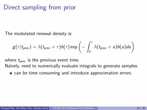
The modulated renewal density is:
g(τ |tprev ) = λ(tprev + τ)h(τ) exp
(−∫ τ
0
λ(tprev + u)h(u)du
)where tprev is the previous event time.Naıvely, need to numerically evaluate integrals to generate samples.
can be time consuming and introduce approximation errors.
Vinayak Rao, Yee Whye Teh (Gatsby Unit) MCMC for Continuous Time Systems 22 / 40

Sampling via uniformizationAssume the intensity function λ(t) and the hazard function h(τ)are bounded
∃Ω ≥ maxt,τ
h(τ)λ(t)
Sample E = E0 = 0,E1,E2, . . . from a Poisson process withrate Ω.Let Y0 = 0,Y1,Y2, . . . be an integer-valued Markov chain onthe times in E , where each Yi either equals Yi−1 or i .
I Yi = Yi−1 → reject Ei ,I Yi = i → keep Ei .
Ei − EYi: time since the last accepted event. For i > j ≥ 0,
define
p(Yi = i |Yi−1 = j) =h(Ei − Ej )λ(Ej )
Ω
Define G = Ei ∈ E s.t. Yi = i.Vinayak Rao, Yee Whye Teh (Gatsby Unit) MCMC for Continuous Time Systems 23 / 40

Sampling via uniformization
LemmaFor any Ω ≥ maxt,τ h(τ)λ(t), G is a sample from a modulatedrenewal process with hazard h(·) and modulating intensity λ(·).
Vinayak Rao, Yee Whye Teh (Gatsby Unit) MCMC for Continuous Time Systems 24 / 40
Sampling via uniformization
0 20 40 60 80 1000
0.05
0.1
0.15
0.2
Inte
nsity
Time
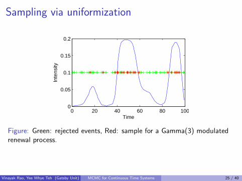
Figure: Green: rejected events, Red: sample for a Gamma(3) modulatedrenewal process.
Vinayak Rao, Yee Whye Teh (Gatsby Unit) MCMC for Continuous Time Systems 25 / 40

Reduction to thinning of Poisson processes
For a Poisson process, the hazard function is a constant:
h(τ) = h
Then, the transition probabilities of the Markov chain becomes:
p(Yi = i |Yi−1 = j) =hλ(Ej )
Ω
This reduces to independent thinning [Adams et al., 2009].
Vinayak Rao, Yee Whye Teh (Gatsby Unit) MCMC for Continuous Time Systems 26 / 40
Inference
Given a set of event times G , obtain sample from the modulatingfunction λ(·) (and hyperparameters).
As before, directly sampling from the GP posterior is impossible.
Introduce the rejected events as auxiliary variables and proceed byalternately sampling the rejected events given G and the intensityfunction, and then the intensity function given G and rejected events.
Vinayak Rao, Yee Whye Teh (Gatsby Unit) MCMC for Continuous Time Systems 27 / 40

InferenceAssume the modulating function λ(t) is known for all t.
In the interval (Gi−1,Gi ), events from a rate Ω Poisson process wererejected with probability:
1− λ(t)h(t − Gi−1)
Ω
Under the posterior, these rejected events are distributed as aninhomogeneous Poisson process with rate:
Ω− λ(t)h(t − Gi−1)
Catch: we know λ(t) only at a discrete set of times. Use thinningmethod of GP Cox processes [Adams et al., 2009].
Vinayak Rao, Yee Whye Teh (Gatsby Unit) MCMC for Continuous Time Systems 28 / 40

InferenceAssume the modulating function λ(t) is known for all t.
In the interval (Gi−1,Gi ), events from a rate Ω Poisson process wererejected with probability:
1− λ(t)h(t − Gi−1)
Ω
Under the posterior, these rejected events are distributed as aninhomogeneous Poisson process with rate:
Ω− λ(t)h(t − Gi−1)
Catch: we know λ(t) only at a discrete set of times. Use thinningmethod of GP Cox processes [Adams et al., 2009].
We resample the GP on the events and the rejected points using ellip-tical slice sampling [Murray et al., 2010].
Vinayak Rao, Yee Whye Teh (Gatsby Unit) MCMC for Continuous Time Systems 28 / 40
Computational considerations
Complexity: O(N3), where N = |G |+ 2|E |, |G | is the number ofobservations and |E | is the number of rejected points.
For large G , we must resort to approximate inference forGaussian processes [Rasmussen and Williams, 2006].
Question: how do these approximations compare withtime-discretized approximations like [Cunningham et al., 2008]?
Vinayak Rao, Yee Whye Teh (Gatsby Unit) MCMC for Continuous Time Systems 29 / 40

ExperimentsThree synthetic datasets generated by modulating a Gamma(3)renewal process.
λ1(t) = 2 exp(t/5) + exp(−((t − 25)/10)2, t ∈ [0, 50]: 44 events
λ2(t) = 5 sin(t2) + 6, t ∈ [0, 5]: 12 events
λ3(t): a piecewise linear function, t ∈ [0, 100]: 153 events
Three settings of our model and a strawman:
with the shape parameter fixed to 1 (MRP Exp),
with the shape parameter fixed to 3 (MRP Gam3),
with a hyperprior on the shape parameter (MRP Full),
an approximate discrete time sampler on a regular grid coveringthe interval, all intractable integrals were approximatednumerically.
Vinayak Rao, Yee Whye Teh (Gatsby Unit) MCMC for Continuous Time Systems 30 / 40

Experiments
0 10 20 30 40 50−0.5
0
0.5
1
1.5
2
2.5
3
Inte
nsity
TruthMRP ExpMRP Gam3MRP FullDisc100
0 1 2 3 4 5−2
0
2
4
6
8
10
12
0 20 40 60 80 100
0
1
2
3
1 2 3 4 50
0.05
0.1
0.15
0.2
1 2 3 4 50
0.05
0.1
0.15
0.2
1 2 3 4 50
0.1
0.2
0.3
0.4
Figure: Synthetic datasets 1-3: Posterior mean intensities (top) andGamma shape posteriors (bottom). Results from 5000 MCMC samplesafter a burn-in of 1000 samples.
Vinayak Rao, Yee Whye Teh (Gatsby Unit) MCMC for Continuous Time Systems 31 / 40

Experiments
MRP Exp MRP Gam3 MRP Full Disc25 Disc100
l2 error 7.85 3.19 2.55 4.09 2.43log pred. -47.55 -38.07 -37.37 -41.65 -41.02
l2 error 141.01 56.22 58.44 91.32 57.9
log pred. -3.70 -2.95 -3.28 -5.25 -3.85
l2 error 82.03 11.42 13.44 122.34 38.05
log pred. -89.88 -48.28 -48.57 87.17 -55.80
Table: l2 distance from the truth and mean log predictive probabilities oftest sets for synthetic datasets 1 (top) to 3 (bottom).
Vinayak Rao, Yee Whye Teh (Gatsby Unit) MCMC for Continuous Time Systems 32 / 40

Experiments
Dataset: the coal mine disaster dataset, recording the dates of aseries of 191 coal mining disasters (each of which killed ten or moremen [Jarrett, 1979]).
1850 1900 1950−1
0
1
2
3
4
Inte
nsity
1850 1900 1950−1
0
1
2
3
4
1 1.5 20
0.05
0.1
0.15
0.2
Figure: Left: posterior mean of the intensity function. The posterior forshape parameter was close to 1. Middle and right: results after deletingevery alternate event.
Vinayak Rao, Yee Whye Teh (Gatsby Unit) MCMC for Continuous Time Systems 33 / 40

ExperimentsDataset: neural spike train recorded from grasshopper auditoryreceptor cells [Rokem et al., 2006].
0 500 1000 15001.5
2
2.5
3
Time (ms) 1 1.5 20
0.1
0.2
Figure: Left: Posterior mean intensity for neural data with 1 standarddeviation error bars. Superimposed is the log stimulus (scaled andshifted). Right: Posterior over the gamma shape parameter.
Vinayak Rao, Yee Whye Teh (Gatsby Unit) MCMC for Continuous Time Systems 34 / 40

ExperimentsWe compare our uniformization based blocked Gibbs sampler withthe sampler of [Adams et al., 2009].
Synthetic dataset 1
Mean ESS Minimum ESS Time(sec)
Gibbs 93.45± 6.91 50.94± 5.21 77.85
MH 56.37± 10.30 19.34± 11.55 345.44
Coalmine dataset
Mean ESS Minimum ESS Time(sec)
Gibbs 53.54± 8.15 24.87± 7.38 282.72
MH 47.83± 9.18 18.91± 6.45 1703
Table: Sampler comparisons. Numbers are per 1000 samples.
Besides mixing faster our sampler:
is simpler and more natural to the problem,
does not require any external tuning.Vinayak Rao, Yee Whye Teh (Gatsby Unit) MCMC for Continuous Time Systems 35 / 40

Conclusions
The idea of uniformization relates more complicated continuoustime discrete state processes to the basic Poisson process.
We demonstrated how this connection can be used to developtractable models and efficient MCMC inference schemes.
We can look into extending the models we discussed here:I renewal processes with unbounded hazard rates,I semi-Markov jump processes,I inhomogeneous MJPs, MJPs with infinite state spaces etc.
Other applications we wish to study, such as survival analysis,queuing systems etc.
Vinayak Rao, Yee Whye Teh (Gatsby Unit) MCMC for Continuous Time Systems 36 / 40

Bibliography IAdams, R. P., Murray, I., and MacKay, D. J. C. (2009).
Tractable nonparametric Bayesian inference in Poisson processes with gaussian process intensities.In Bottou, L. and Littman, M., editors, Proceedings of the 26th International Conference on Machine Learning (ICML),pages 9–16, Montreal. Omnipress.
Cohn, I., El-Hay, T., Friedman, N., and Kupferman, R. (2010).
Mean field variational approximation for continuous-time bayesian networks.J. Mach. Learn. Res., 11:2745–2783.
Cunningham, J. P., Yu, B. M., Shenoy, K. V., and Sahani, M. (2008).
Inferring neural firing rates from spike trains using gaussian processes.In Advances in Neural Information Processing Systems,20.
El-Hay, T., Friedman, N., and Kupferman, R. (2008).
Gibbs sampling in factorized continuous-time Markov processes.In UAI, pages 169–178.
Fan, Y. and Shelton, C. R. (2008).
Sampling for approximate inference in continuous time Bayesian networks.In Tenth International Symposium on Artificial Intelligence and Mathematics.
Fearnhead, P. and Sherlock, C. (2006).
An exact Gibbs sampler for the Markov-modulated Poisson process.Journal Of The Royal Statistical Society Series B, 68(5):767–784.
Hobolth, A. and Stone, E. A. (2009).
Simulation from endpoint-conditioned, continuous-time Markov chains on a finite state space, with applications tomolecular evolution.Ann Appl Stat, 3(3):1204.
Vinayak Rao, Yee Whye Teh (Gatsby Unit) MCMC for Continuous Time Systems 37 / 40

Bibliography II
Jarrett, B. Y. R. G. (1979).
A note on the intervals between coal-mining disasters.Biometrika, 66(1):191–193.
Jensen, A. (1953).
Markoff chains as an aid in the study of Markoff processes.Skand. Aktuarietiedskr., 36:87–91.
Murray, I., Adams, R. P., and MacKay, D. J. (2010).
Elliptical slice sampling.JMLR: W&CP, 9:541–548.
Nodelman, U., Koller, D., and Shelton, C. (2005).
Expectation propagation for continuous time Bayesian networks.In Proceedings of the Twenty-first Conference on Uncertainty in AI (UAI), pages 431–440, Edinburgh, Scottland, UK.
Nodelman, U., Shelton, C., and Koller, D. (2002).
Continuous time Bayesian networks.In Proceedings of the Eighteenth Conference on Uncertainty in Artificial Intelligence (UAI), pages 378–387.
Opper, M. and Sanguinetti, G. (2007).
Variational inference for Markov jump processes.In NIPS.
Rao, V. and Teh, Y. W. (2011a).
Fast MCMC sampling for Markov jump processes and continuous time Bayesian networks.In Proceedings of the International Conference on Uncertainty in Artificial Intelligence.
Vinayak Rao, Yee Whye Teh (Gatsby Unit) MCMC for Continuous Time Systems 38 / 40
Bibliography III
Rao, V. and Teh, Y. W. (2011b).
Gaussian process modulated renewal processes.In Advances in Neural Information Processing Systems 23.
Rasmussen, C. E. and Williams, C. K. I. (2006).
Gaussian Processes for Machine Learning.MIT Press.
Rokem, A., Watzl, S., Gollisch, T., Stemmler, M., Herz, A. V. M., Watzl, S., Gollisch, T., Stemmler, M., and Herz, A.
V. M. (2006).Spike-Timing Precision Underlies the Coding Efficiency of Auditory Receptor Neurons.Journal of Neurophysiology, pages 2541–2552.
Vinayak Rao, Yee Whye Teh (Gatsby Unit) MCMC for Continuous Time Systems 39 / 40

Algorithm 1 Blocked Gibbs sampler for GP-modulated renewal pro-cess on the interval [0,T ]
Input: Set of event times G , set of thinned times Gprev and l instanti-ated at G ∪ Gprev .Output: A new set of thinned times Gnew and a new instantiationlG∪Gnew
of the GP on G ∪ Gnew .
1: Sample A ⊂ [0,T ] from a Poisson process with rate Ω.2: Sample lA|lG∪Gprev
.3: Thin A, keeping element a ∈ A ∩ [Gi−1,Gi ] with probability(
1− λσ(l(a))h(a−Gi−1)Ω
).
4: Let Gnew be the resulting set and lGnewbe the restriction of lA to
this set. Discard Gprev and lGprev.
5: Resample lG∪Gnewusing, for example, elliptical slice sampling.
Vinayak Rao, Yee Whye Teh (Gatsby Unit) MCMC for Continuous Time Systems 40 / 40