effects of various uncertainty sources on automatic...
TRANSCRIPT

Effects of Various Uncertainty Sources
on Automatic Generation Control
Systems
D. Apostolopoulou, Y. C. Chen, J. Zhang,A. D. Domınguez-Garcıa, and P. W. Sauer
University of Illinois at Urbana-Champaign
May 3, 2013
(UIUC) May 3, 2013 1 / 28

Outline
1 Introduction
2 Power System and AGC Models
3 Numerical Results
4 Concluding Remarks
(UIUC) May 3, 2013 2 / 28

Outline
1 Introduction
2 Power System and AGC Models
3 Numerical Results
4 Concluding Remarks
(UIUC) May 3, 2013 3 / 28

Demand and Generation Balance
32
30
28
26
24
22
20
00 01 02 03 04 05 06 07 08 09 10 11 12 13 14 15 16 17 18 19 20 21 22 23Hour
Actual Demand (GW)Day Ahead Demand Forecast
Available Resources Forecast (GW)
Source: www.caiso.com
(UIUC) May 3, 2013 4 / 28

Who is in charge?The Balancing Authority (BA) is the responsible entity that integratesresource plans ahead of time, maintains load-interchange-generationbalance within a BA Area, and supports interconnection frequency in realtime
Source: www.nerc.com
(UIUC) May 3, 2013 5 / 28

Frequency deviation from nominal value
- +
60
DEMAND SUPPLY
Losses
Power
Generated Load
Frequency
Decrease Increase
Source: www.nerc.com
(UIUC) May 3, 2013 6 / 28

Control Processes
105
1041 10 10
310
2
primary control
secondary control
tertiary control
optimal power flow
unit commitment
time(s)
1 sec 1 min 1 hour 1 day
{
Lo
ad
Fre
qu
en
cy C
on
tro
l
(UIUC) May 3, 2013 7 / 28

Load Frequency Control
Source: http://www.e-control.at/en/businesses/electricity/electricity-market/balancing-energy
(UIUC) May 3, 2013 8 / 28

Automatic Generation Control (AGC)
Role of AGC in power systems
To hold system frequency at or very close to a specified nominalvalue.
To maintain the correct value of interchange power between controlareas.
AGC implementation
The AGC accepts measurements of the real power interchangebetween areas, the area’s frequency and the generator’s output asinput signals from field devices.
The output control signals represent the shift in the area’s generationrequired to restore frequency and net interchange to the desiredvalues.
(UIUC) May 3, 2013 9 / 28

Challenges in AGC
Deepening penetration of renewable resources, which are highlyvariable and intermittent.
6
Renewable Portfolio Standards
State renewable portfolio standard
State renewable portfolio goal
www.dsireusa.org / February 2010
Solar water heating eligible * † Extra credit for solar or customer-sited renewables
Includes non-renewable alternative resources
WA: 15% x 2020*
CA: 33% x 2020
NV: 25% x 2025*
AZ: 15% x 2025
NM: 20% x 2020 (IOUs) 10% x 2020 (co-ops)
HI: 40% x 2030
Minimum solar or customer-sited requirement
TX: 5,880 MW x 2015
UT: 20% by 2025*
CO: 20% by 2020 (IOUs) 10% by 2020 (co-ops & large munis)*
MT: 15% x 2015
ND: 10% x 2015
SD: 10% x 2015
IA: 105 MW
MN: 25% x 2025 (Xcel: 30% x 2020)
MO: 15% x 2021
WI: Varies by utility; laog 5102 x %01
MI: 10% + 1,100 MW x 2015*
OH: 25% x 2025†
ME: 30% x 2000 New RE: 10% x 2017
NH: 23.8% x 2025
MA: 15% x 2020 + 1% annual increase
(Class I RE)
RI: 16% x 2020
CT: 23% x 2020
NY: 29% x 2015
NJ: 22.5% x 2021
PA: 18% x 2020†
MD: 20% x 2022
DE: 20% x 2019*
DC: 20% x 2020
VA: 15% x 2025*
NC: 12.5% x 2021 (IOUs) 10% x 2018 (co-ops & munis)
VT: (1) RE meets any increase in retail sales x 2012;
(2) 20% RE & CHP x 2017
KS: 20% x 2020
OR: 25% x 2025 (large utilities)* 5% - 10% x 2025 (smaller utilities)
IL: 25% x 2025 WV: 25% x 2025*†
29 states + DC have an RPS (6 states have goals)
DC
0
OW
Source: www.dsireusa.org – April 2013
(UIUC) May 3, 2013 10 / 28

Challenges in AGC
Highly automated system, which lead to increase noised signals thatare measured and transmitted to the AGC.
Source: http://www.electronicproducts.com
(UIUC) May 3, 2013 11 / 28

Proposed Framework
We propose a framework to evaluate the effects of uncertainty in AGC byexplicitly representing the
system dynamics
network effects
uncertainty sources
We approximate the probability distribution function of systemcharacteristics to investigate if the AGC mechanism is functional
(UIUC) May 3, 2013 12 / 28

Outline
1 Introduction
2 Power System and AGC Models
3 Numerical Results
4 Concluding Remarks
(UIUC) May 3, 2013 13 / 28

Synchronous Generating Units
For the timescales of interest we chose a 4-state model for thesynchronous generators that includes the mechanical equations andthe governor dynamics
T ′
doi
dE′
qi
dt= −
Xdi
X ′
di
E′
qi−
Xdi −X ′
di
X ′
di
cos(δi − θi) + Efd0i (1)
dδi
dt= ωi − ωs (2)
2Hi
ωs
dωi
dt= PSVi
−
E′
qi
X ′
di
Vicos(δi − θi) (3)
+Xqi −X ′
di
2X ′
diXqi
V 2
i sin(2(δi − θi))−Di(ωi − ωs)
TSVi
dPSVi
dt= −PSVi
+ PCi−
1
RDi
(ωi
ωs
− 1)
(4)
We denote x = [E′
q1, δ1, ω1, PSV1
, . . . , E′
qI, δI , ωI , PSVI
]T
(UIUC) May 3, 2013 14 / 28

Network
Power flow equations
P si + Pw
i − P di =
n∑
k=1
ViVk(
Gikcos(θi − θk) +Biksin(θi − θk))
(5)
Qsi −Qd
i =n∑
k=1
ViVk(
Giksin(θi − θk)−Bikcos(θi − θk))
(6)
where P si =
E′
qi
X′
di
Vicos(δi − θi)−Xqi
−X′
di
2X′
diXqi
V 2
i sin(2(δi − θi)) and
Qsi =
E′
qi
X′
di
Vicos(δi − θi)−1
X′
di
V 2
i cos2(δi − θi)−
1
XqiV 2
i sin2(δi − θi)
We denote y = [θ1, V1, . . . , θn, Vn]T , P d = [P d
1, . . . , P d
n ]T and
Qd = [Qd1, . . . , Qd
n]T
(UIUC) May 3, 2013 15 / 28

AGC Model
Area control errorACE = b(f − fnom) (7)
Frequency
f =
n∑
i=1
γi
(
fnom +1
2π
dθi
dt
)
(8)
where γi some weighting factors with∑n
i=1γi = 1
AGC control
dz
dt= −z −
1
η2ACE +
I∑
i=1
P si (9)
PCi= κi z (10)
We denote u = [PC1, . . . , PCI
]T
(UIUC) May 3, 2013 16 / 28

Wind generation and communication noise
The wind generation model at node i
˙PWi= γ1i PWi
+ γ2i vi + γ3i (11)
dvi = ai vi dt+ bi dWt (12)
Uncertainty in the measurements Γ of the vector Γ , containing thefrequency and the generators’ output, is modeled as Gaussian whitenoise ηΓ
Γ = Γ + ηΓ (13)
The area control error as well as the AGC mechanism is affected byηΓ as may be seen in (10)
We denote PW = [PW1, . . . , PWn ]
T and v = [v1, . . . , vn]T
(UIUC) May 3, 2013 17 / 28

System Model
The system dynamic behavior is described by a set of differentialalgebraic equations
x = f(x, y, u) (14)
z = h(x, y, y, z) (15)
u = k(z) (16)
0 = g(x, y, PL, PW ) (17)
We linearize the system along a nominal trajectory and obtain
dXt = AXtdt+BdWt (18)
where X = [∆x,∆z,∆PW ,∆v]T
(UIUC) May 3, 2013 18 / 28

Calculation of desired moments
Generator of the stochastic process X
(Lψ)(X) :=∂ψ(X)
∂XAX +
1
2Tr
(
B∂2ψ(X)
∂X2BT
)
(19)
The evolution of the expected value of ψ(X) is governed by Dynkin’sformula
dE[ψ(Xt)]
dt= E[(Lψ)(Xt)] (20)
Cross-moments evolution
dΣ(t)
dt= AΣ(t) + Σ(t)AT +BBT (21)
E[XtXTt ] = Σ(t) + E[Xt]E[Xt]
T (22)
(UIUC) May 3, 2013 19 / 28

Outline
1 Introduction
2 Power System and AGC Models
3 Numerical Results
4 Concluding Remarks
(UIUC) May 3, 2013 20 / 28
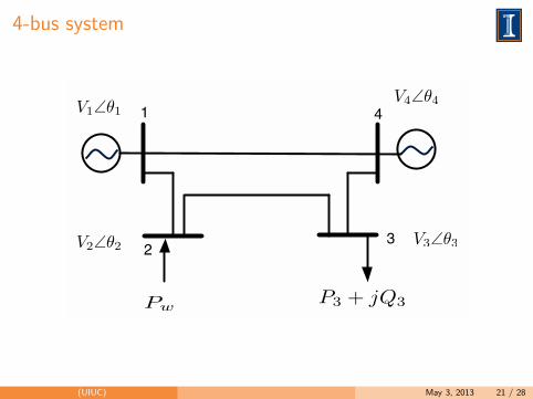
4-bus system
1 4
23
V1∠θ1
V2∠θ2
Pw
P3 + jQ3
V3∠θ3
V4∠θ4
(UIUC) May 3, 2013 21 / 28

Deterministic case: Wind change by 0.1pu
0 200 400 600 800 1000−0.5
0
0.5
1
rad/s
time (s)
∆ω1
∆ω4
0 200 400 600 800 1000−0.2
−0.15
−0.1
−0.05
0
pu
time (s)
∆PSV
1
∆PSV
4
(UIUC) May 3, 2013 22 / 28

Incorporating uncertainty
Variation of wind generation
0 10 20 30 40 50 60 70 80−0.02
−0.01
0
0.01
0.02
pu
time (s)
The variation in system’s frequency may be expressed as a linearcombination of the system states
∆f = CXt (23)
The mean value and second moment of ∆f are
E[∆f ] = CE[Xt] (24)
E[∆f2] = CE[XtXTt ]C
T (25)
(UIUC) May 3, 2013 23 / 28

Mean and Second moment of ∆f
0 20 40 60 80 100 120−0.2
−0.15
−0.1
−0.05
0
0.05
Hz
time (s)
Dynkin’s formulaMonte Carlo
! "! #! $! %! &!! &"!!
!'!&
!'!"
!'!(
Hz2
time (s)
)! &!! &&! &"!
!
"
#
*+&!!$
,-./0.12+3456789
:4.;<+=9584
(UIUC) May 3, 2013 24 / 28

Increasing the wind penetration
0 20 40 60 80 100 1200
2
4
6x 10⁻⁶
Hz2
time (s)
PW0
2PW0
(UIUC) May 3, 2013 25 / 28

Outline
1 Introduction
2 Power System and AGC Models
3 Numerical Results
4 Concluding Remarks
(UIUC) May 3, 2013 26 / 28

Concluding Remarks and Applications
We proposed a methodology of propagating any uncertainty in eitherPW or noise in the communication channels ηΓ and study their effecton the AGC signals u and eventually on the system performance
We may use this framework to
◮ to detect, in a timely manner, the existence of a cyber attack, bycomputing the system frequency statistics
◮ determine which buses are more critical if noise is inserted in themeasurements
◮ obtain upper bounds for the frequency variation, by using Chebyshev’sinequality, and investigate if they meet the frequency regulation criteria
(UIUC) May 3, 2013 27 / 28

Thank you!
(UIUC) May 3, 2013 28 / 28