location uncertainty a probabilistic solution for ... location uncertainty... · location...

Location Uncertainty – A Probabilistic solution for Automatic Train Control of 11

Location Uncertainty – A Probabilistic Solution For Automatic Train Control

Monish Sengupta, Principal Consultant, Ricardo Rail

Professor Benjamin Heydecker, University College London

Dr. Daniel Woodland, Ricardo Rail

SUMMARY New train control systems rely mainly on Automatic Train Protection (ATP) and Automatic Train Operation (ATO) to dynamically control the speed and hence performance. The ATP and the ATO form the vital element within CBTC (Communication Based Train Control) and within the ERTMS (European Rail Traffic Management System) system architectures. As we move towards GOA4 (Grade of Automation 4 – unmanned operation) railways need greater control over the speed, timing and location of trains. Reliable and accurate measurement of train location, speed and acceleration are hence vital to the operation of modern train control systems.

In the past, all CBTC and ERTMS system have deployed a balise or equivalent to correct the uncertainty element of the train location. Typically a CBTC train is allowed to miss only one balise on the track, after which the Automatic Train Protection (ATP) system applies the emergency brake to halt the service. This is because the location uncertainty, which grows within the train control system over time and as the train moves, cannot tolerate missing more than a defined number of balises. Balises contribute a significant amount towards wayside maintenance and studies have shown that balises on the track also forms a constraint for future track layout change and change in speed profile.

The Author has been undertaking studies at the University College London to investigate the causes of the location uncertainty that is currently experienced and consider whether it is possible to identify an effective filter to ascertain, in conjunction with appropriate sensors, more accurate speed, distance and location for a CBTC driven train without the need of any external balises. An appropriate sensor fusion algorithm and intelligent sensor selection methodology can also be deployed to ascertain the railway location and speed measurement at its highest precision. Similar techniques are already in use in aviation, satellite, submarine and other navigation systems.

Developing a model for the speed control and the use of Kalman filters is a key element in this research. This paper will summarise the research undertaken and its significant findings, highlighting the potential for introducing alternative approaches to train positioning that would enable removal of all trackside location correction balises, leading to huge reduction in maintenances and more flexibility in future track design.

1 INTRODUCTION

Train navigation system can be broadly specified in three categories. These are: dead reckoning; radio location and inertial navigation. It has been established that it is not possible to obtain the optimal location from any one type of navigation system. The sensors attributed towards dead reckoning are tachometers, Doppler radars and balises. Radio location uses triangulation of time stamped radio transmission to determine train location. Inertial navigation, which is the only self-contained navigation, can be achieved by on-board accelerometers and gyroscopes.

While wheel tachometers are accurate sensors, often wheel slipping and sliding can lead to huge noise in the sensor output especially where the tachometer is fitted to the motored/braked axle. Dopplers on the other hand can be more accurate as it does not depend on the wheel slip or slide. The velocity data is derived from the Doppler sensor [1] as


𝑭𝒅 = 𝟐𝒗𝑪𝒐𝒔𝜰/𝝀 (1)

Where

𝒗 = 𝒕𝒓𝒂𝒊𝒏 𝒔𝒑𝒆𝒆𝒅 𝒓𝒆𝒍𝒂𝒕𝒊𝒗𝒆 𝒕𝒐 𝒕𝒉𝒆 𝒈𝒓𝒐𝒖𝒏𝒅

𝐹𝑑 = 𝐷𝑜𝑝𝑝𝑙𝑒𝑟 𝑓𝑟𝑒𝑞𝑢𝑒𝑛𝑐𝑦 𝑠ℎ𝑖𝑓𝑡

𝛶 = 𝑟𝑎𝑑𝑖𝑎𝑡𝑖𝑜𝑛 𝑎𝑛𝑔𝑙𝑒

𝜆 = 𝑡𝑟𝑎𝑛𝑠𝑚𝑖𝑡𝑡𝑒𝑑 𝑐𝑎𝑟𝑟𝑖𝑒𝑟 𝑤𝑎𝑣𝑒𝑙𝑒𝑛𝑔𝑡ℎ

Location and acceleration can be derived by integrating and differentiating the velocity achieved from equation (1). As the doppler can have radar scatter error and the location is derived by integrating the velocity 𝒗, noise in the location data will also get integrated and hence will grow with time. Radio locations often have black spots and prove not to be extremely reliable [3].

Being self-contained, inertial navigation does not need any external correction. However inertial navigation sensors record the acceleration of the train and integrate it to obtain the speed and the location. Double integration of the acceleration data leads to huge noise in the location estimation which grows over time. This can lead to unsafe situation where the train will need to ultimately apply emergency brakes.

2 CURRENT ARCHITECTURE

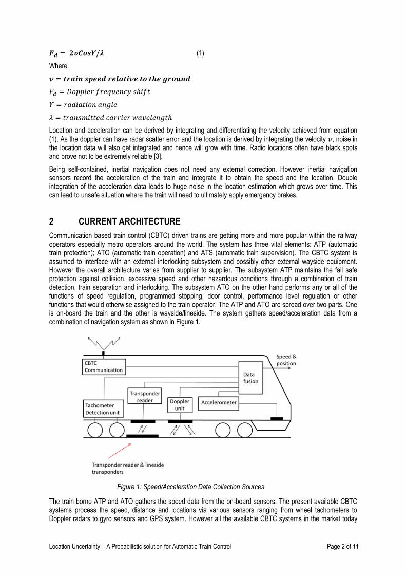
Communication based train control (CBTC) driven trains are getting more and more popular within the railway operators especially metro operators around the world. The system has three vital elements: ATP (automatic train protection); ATO (automatic train operation) and ATS (automatic train supervision). The CBTC system is assumed to interface with an external interlocking subsystem and possibly other external wayside equipment. However the overall architecture varies from supplier to supplier. The subsystem ATP maintains the fail safe protection against collision, excessive speed and other hazardous conditions through a combination of train detection, train separation and interlocking. The subsystem ATO on the other hand performs any or all of the functions of speed regulation, programmed stopping, door control, performance level regulation or other functions that would otherwise assigned to the train operator. The ATP and ATO are spread over two parts. One is on-board the train and the other is wayside/lineside. The system gathers speed/acceleration data from a combination of navigation system as shown in Figure 1.

The train borne ATP and ATO gathers the speed data from the on-board sensors. The present available CBTC systems process the speed, distance and locations via various sensors ranging from wheel tachometers to Doppler radars to gyro sensors and GPS system. However all the available CBTC systems in the market today

Figure 1: Speed/Acceleration Data Collection Sources


require some form of third party authentication for their location data, due to the huge accumulation of noise as explained earlier. This can be either in the form of wayside balises or loops.

ERTMS follows a very similar architecture to that of CBTC, as explained above. For ERTMS level 2 and above, the signalling information is transmitted to the train via radio link. This radio link uses GSM-R data radio (part of ERTMS) [5].

3 CONSTRAINTS AS A RESULT

In order to get rid of this error, we provide external wayside balises. On the Victoria line, they are located every 120m or less which ensures that the train will continue in the event of single balise failure. However in the event of consecutive balise failure, the on-board ATP applies the emergency brake. The distance between balises is dependent on line speed and features of the railway e.g. signals positions, convergences and divergences, station stops, reversing and berthing locations. Typically there are two balises on the approach to a signal and up to six in a platform that is designated as a berthing location with a reversing move. Although the Jubilee and Northern Line are strictly not a CBTC system rather a TBTC system, the equivalent position reference occurs every 25m approximately, via transpositions in a trackside loop. The reason for this is the inherent inability to measure the state noise in any coherent system. This noise is random and is assumed to have a Gaussian distribution.

The need for the balise gives rise to:

1. More lineside assets leading to extra equipment cost and maintenance

2. Excessive cost or restrictions associated with reconfiguring or renewing the track layout, or

reconfiguring the location of a balise once commissioned.

3. Extra on-board sensors, mounted on the underframe, which at times becomes difficult - especially for

retrofitting existing stock

4. Enhanced safety requirements to ensure correct balise data

5. Potential for emergency brake application, impacting performance, in the event of faulty or missing

balises

6. As the system will assume worst case stopping in case of a missing balise , there has to be an added

safety margin when considering train separation and train approaching a junction or buffer or making a

station stop, especially with platform edge doors.,

The above restrictions and constraints led to this study, to understand the source of this location uncertainty and consider a possible mean to solve it without requirement for balises.

4 APPLICATION OF KALMAN FILTER

The state equation for any random process can be represented as (2)

𝐱𝐭+𝟏 = ∅𝐭𝐱𝐭 + 𝐰𝐭 (2)

We assume the state of a system 𝐱𝐭 at time t changes to a different state 𝐱𝐭+𝟏 at time t+1 due to the presence of a force. In our case the train will change its position and speed due to the presence of the force acceleration or

deceleration. While the state changes between t and t+1, there will be an accumulation of noise 𝐰𝐭 which is inherent to any state model. Therefore the state at t+1 will look like equation (2).

The measurement of the above process can be represented as

𝐳𝐭 = 𝐇𝐭𝐱𝐭 + 𝐯𝐭 (3)


Where,

𝐱𝐭 – process state vector at time t

∅𝐭 – matrix relating to xt and xt+1 or state matrix

𝐰𝐭 – white sequence with known covariance structure. This is the input white noise contribution to the state vector.

𝐳𝐭 – measurement matrix at time t

𝐇𝐭 – ideal noiseless connection between the state and the observation or measurement matrix

𝐯𝐭 –observation white sequence with known covariance structure.

𝐰𝐭 and 𝐯𝐭 assumed to have zero cross-correlation

Covariance measures the degree to which two variables change or vary together (i.e. co-vary). On one hand, the covariance of two variables is positive if they vary together in the same direction relative to their expected values (i.e. if one variable moves above its expected value, then the other variable also moves above its expected value). On the other hand, if one variable tends to be above its expected value when the other is below its expected value, then the covariance between the two variables is negative. If there is no linear dependency between the two variables, then the covariance is 0. We represent an expected value of a particular variable as E[y], where y is any random variable.

The covariance matrix for the noise wt and vt are given by:

𝐄 [𝐰𝐭𝐰𝐢𝐓] = {

𝐐𝐭, 𝐢 = 𝐭𝟎, 𝐢 ≠ 𝐭

(4)

𝐄 [𝐯𝐭𝐯𝐢𝐓] = {

𝐑𝐭, 𝐢 = 𝐭𝟎, 𝐢 ≠ 𝐭

(5)

𝐄 [𝐰𝐭𝐯𝐢𝐓] = 𝟎 for all t and i (6)

Looking into the above state equation (2), we know there is an inherent noise in the state and its corresponding observation has more noise, especially if the location is derived from INS sensors or dead reckoning sensors, along with the integration of the acceleration data to derive the location, the noise too gets integrated. This noise grows over the time and hence we need external reference such as balise to negate or compensate the noise.

Let us now apply Kalman filter to the above noisy state. To carry out the steps of a Kalman filter, we choose an apriori estimate �̂�𝟎

− and 𝐏𝟎−. In this notation, the ‘hat’ denotes the estimate, the super minus is our best apriori

estimate prior to t = 1.

Step 1: Compute Kalman Gain

𝐊𝐭 = 𝐏𝐭−𝐇𝐭

𝐓 (𝐇𝐭𝐏𝐭−𝐇𝐭

𝐓 + 𝐑𝐭) −𝟏 (7)

Step 2: Update estimate with observation z (equation 3) at time t:

�̂�𝐭 = �̂�𝐭− + 𝐊𝐭(𝐙𝐭 − 𝐇𝐭�̂�𝐭

−) (8)

Step 3: Compute error covariance for updated estimate:

𝐏𝐭 = (𝐈 − 𝐊𝐭𝐇𝐭)𝐏𝐭−(𝐈 − 𝐊𝐭𝐇𝐭 ) 𝐓 + 𝐊𝐑𝐊𝐓 (9)


Step 4: Project ahead:

�̂�𝐭+𝟏− = ∅𝐭�̂�𝐭 (10)

𝐏𝐭+𝟏− = ∅𝐭𝐏𝐭∅𝐭

𝐓 + 𝐐𝐭 (11)

Repeat step 1 to 4 till time t. Where the associated state error covariance matrix 𝐏𝐭 at time t can be represented as:

𝐏𝐭 = 𝐄[𝐞𝐭𝐞𝐤𝐓] = 𝐄[(𝐱𝐭 − �̂�𝐭)(𝐱𝐭 − �̂�𝐭) 𝐓] (12)

The state in the case of a moving train is:

(

𝑥𝑡

�̇�𝑡

�̈�𝑡

) = (1 ∆𝑡 ∆𝑡/20 1 ∆𝑡0 1 1

) (

𝑥𝑡−1

�̇�𝑡−1

�̈�𝑡−1

) + (

𝛼𝑡−1

𝛽𝑡−1

𝛾𝑡−1

)

Where the state noise 𝒘𝒕−𝟏 = (

𝛼𝑡−1

𝛽𝑡−1

𝛾𝑡−1

) (13)

5 METHODOLOGY

We build a simulation model in MATLAB for a train to:

Travel a distance: 3200m

Time to take: 150s

Initial rate of acceleration: 0.8m/s2

Rate of deceleration: 1.2m/s2

Cruise speed: 40m/s

Approach speed: 20m/s

We set apriori 𝐏𝟎− as [

100 0 00 100 00 0 100

]

and the apriori state �̂�𝟎− = [

000

]

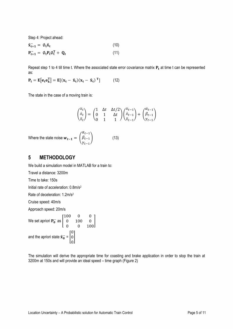
The simulation will derive the appropriate time for coasting and brake application in order to stop the train at 3200m at 150s and will provide an ideal speed – time graph (Figure 2)


In the simulation we also generate a set of observation for location, speed and acceleration with a given standard deviation of noises. We assume the noises to be Gaussian in nature, hence throwing up random numbers with a zero mean. We take these randomly generated numbers as noise and feed into the Kalman filter. In parallel we also generate a true location, speed and acceleration with a little noise, which is the model noise as mentioned in equation (2).

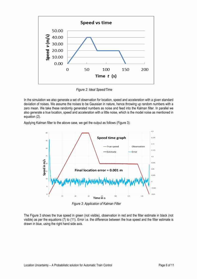
Applying Kalman filter to the above case, we get the output as follows (Figure 3):

The Figure 3 shows the true speed in green (not visible), observation in red and the filter estimate in black (not visible) as per the equations (7) to (11). Error i.e. the difference between the true speed and the filter estimate is drawn in blue, using the right hand side axis.

Figure 2: Ideal Speed/Time

Figure 3: Application of Kalman Filter


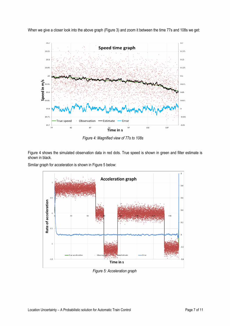
When we give a closer look into the above graph (Figure 3) and zoom it between the time 77s and 108s we get:

Figure 4 shows the simulated observation data in red dots. True speed is shown in green and filter estimate is shown in black.

Similar graph for acceleration is shown in Figure 5 below:

Figure 4: Magnified view of 77s to 108s

Figure 5: Acceleration graph


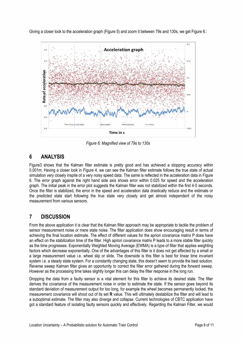
Giving a closer look to the acceleration graph (Figure 5) and zoom it between 79s and 130s, we get Figure 6.:

6 ANALYSIS

Figure3 shows that the Kalman filter estimate is pretty good and has achieved a stopping accuracy within 0.001m. Having a closer look in Figure 4, we can see the Kalman filter estimate follows the true state of actual simulation very closely inspite of a very noisy speed data. The same is reflected in the acceleration data in Figure 6. The error graph against the right hand side axis shows error within 0.025 for speed and the acceleration graph. The initial peak in the error plot suggests the Kalman filter was not stabilized within the first 4-5 seconds. Once the filter is stabilized, the error in the speed and acceleration data drastically reduce and the estimate or the predicted state start following the true state very closely and get almost independent of the noisy measurement from various sensors.

7 DISCUSSION

From the above application it is clear that the Kalman filter approach may be appropriate to tackle the problem of sensor measurement noise or mere state noise. The filter application does show encouraging result in terms of achieving the final location estimate. The effect of different values for the apriori covariance matrix P does have an effect on the stabilization time of the filter. High apriori covariance matrix P leads to a more stable filter quickly as the time progresses. Exponentially Weighted Moving Average (EWMA) is a type of filter that applies weighting factors which decrease exponentially. One of the advantages of this filter is it does not get affected by a small or a large measurement value i.e. wheel slip or slide. The downside is this filter is best for linear time invariant system i.e. a steady state system. For a constantly changing state, this doesn’t seem to provide the best solution. Reverse sweep Kalman filter gives an opportunity to correct the filter error gathered during the forward sweep. However as the processing time takes slightly longer this can delay the filter response in the long run.

Dropping the data from a faulty sensor is a vital element for this filter to achieve its desired state. The filter derives the covariance of the measurement noise in order to estimate the state. If the sensor goes beyond its standard deviation of measurement output for too long, for example the wheel becomes permanently locked, the measurement covariance will shoot out of its set R value. This will ultimately destabilize the filter and will lead to a suboptimal estimate. The filter may also diverge and collapse. Current technologies of CBTC application have got a standard feature of isolating faulty sensors quickly and effectively. Regarding the Kalman Filter, we would

Figure 6: Magnified view of 79s to 130s


like to propose a decentralized Kalman Filter (Figure 7), where we have dedicated filters for each sensor which are periodically fused to achieve a global solution [1].

Decentralised Kalman Filter (Figure 7) also keeps the computational load low.

The greatest challenge for Kalman filter is the apriori state estimate and the apriori process covariance matrix P. This leads to the fact that over-estimating or under-estimating the state and the measurement noise can lead to false state covariance matrix Q and measurement covariance matrix R. This can generate a sub-optimal state estimate and in some cases can lead to filter divergence. Interestingly a complete noise-free state model can lead to a complete collapse of the Kalman filter. The filter gets extremely sluggish and fails to respond to change of state (Figure 8). This suggests a non-zero value of Q is always desirable to keep the filter functioning correctly.

Figure 7: Decentralized Kalman Filter

Figure 8


8 CONCLUSION

The above discussion leads us to believe that Kalman filter, if deployed correctly can achieve stunning result. This will eventually lead to less wayside balises, which in turn means:

1. Savings in maintenance 2. Eliminating train location uncertainty 3. Enhanced performance benefit 4. Ease in design implementation 5. Ease in future track renewal 6. Less impact of wheel slip and slide

However the solution has got quite a few challenges. They are:

1. Modelling the state equation 2. Setting the correct noise profiles (R & Q) 3. Capturing the true sensor noise profile 4. Safety enhancement for the filter software 5. Safety analysis of the overall ATP system architecture with this filter algorithm running in the

background

We are currently examining several derivatives of Kalman filter such as Adaptive Kalman filter, Schmidt Kalman filter and unscented Kalman filter.

Taking into account the need of precise location for a train on the network and to deliver a safe, reliable and accurate filter algorithm and a sensor fusion technique [4], there is much to be gained from the study of the various derivatives of Kalman filter and its applications. The filter is safely implemented in various space and aircraft programmes and other navigation industries.

ABBREVIATIONS AND ACRONYMS

ATO – Automatic Train Operation

ATP – Automatic Train Operation

CBTC – Communication Based Train Control

TBTC – Transmission Based Train Control

ERTMS – European Rail Traffic Management System

GOA – Grade of Automation

GSM – R – Global System of Mobile communication Railway

EWMA – Exponentially weighted Moving Average

INS – Inertial Navigation System

REFERENCES

1. A. Mirabadi, N. Mort, and F. Schmid, “Application of Sensor Fusion to Railway Systems”, Proceedings of the 1996 IEEE/SICE/RSJ International Conference on Multisensor Fusion and Integration for Intelligent Systems, 1996

2. Brown & Hwang, “Introduction to Random Signals and Applied Kalman Filtering”, fourth edition, chapter 5, 2012

3. L.Zhu, B.Ning and H. Jiang, “Train-Ground Communication in CBTC Based on 802.11b: Design and Performance Research”, 2009 International Conference and mobile Computing, 2009


4. J.Dong, D. Zhuang, Y. Huang and J.Fu, “Advances in Multi-Sensor Data Fusion: Algorithms and Applications”, Sensors, 2009

5. Railway Group Guidance Note, “ETCS System Description: GE/GN8605”, Issue One, February 2010

location uncertainty a probabilistic solution for ... location uncertainty... · location...

Documents